Bethe-Heitler signature in proton synchrotron models for gamma-ray bursts

Abstract

We study the effect of Bethe-Heitler (BeHe) pair production on a proton synchrotron model for the prompt emission in gamma-ray bursts (GRBs). The possible parameter space of the model is constrained by consideration of the synchrotron radiation from the secondary BeHe pairs. We find two regimes of interest. 1) At high bulk Lorentz factor, large radius and low luminosity, proton synchrotron emission dominates and produces a spectrum in agreement with observations. For part of this parameter space, a subdominant (in the MeV band) power-law is created by the synchrotron emission of the BeHe pairs. This power-law extends up to few tens or hundreds of MeV. Such a signature is a natural expectation in a proton synchrotron model, and it is seen in some GRBs, including GRB 190114C recently observed by the MAGIC observatory. 2) At low bulk Lorentz factor, small radius and high luminosity, BeHe cooling dominates. The spectrum achieves the shape of a single power-law with spectral index $\alpha=-3/2$ extending across the entire GBM/Swift energy window, incompatible with observations. Our theoretical results can be used to further constrain the spectral analysis of GRBs in the guise of proton synchrotron models.

section [7mm]7mm*[2.7mm].[]

1 Introduction

The emission mechanism at the origin of the observed signal during the prompt phase of GRBs remains unknown. Among the prime contenders are photospheric emission, released when the plasma becomes optically thin (Goodman, 1986; Paczynski, 1986; Mészáros & Rees, 2000; Drenkhahn & Spruit, 2002), and synchrotron emission produced by relativistic particles accelerated by shocks or magnetic reconnection once the flow is optically thin (Rees & Meszaros, 1994; Sari et al., 1996; Daigne & Mochkovitch, 1998; Zhang & Yan, 2011). In addition, protons may also contribute, either directly by synchrotron emission, or indirectly by emission from the secondaries produced in photo-hadronic and photo-pair processes (Asano et al., 2009; Crumley & Kumar, 2013; Florou et al., 2021).

When comparing models to spectral data, the most crucial difference between the aforementioned models are the prediction for the low energy spectral slope $\alpha$, usually associated with the low-energy slope of the Band model (Band et al., 1993). For photospheric emission models, the slope is expected to be around $\alpha=0.4$ (Beloborodov, 2010; Pe’er & Ryde, 2011; Bégué et al., 2013; Parsotan & Lazzati, 2018), unless the ejecta becomes transparent during the acceleration phase (Goodman, 1986; Paczynski, 1986; Bégué & Vereshchagin, 2014; Ryde et al., 2017), in which case a steeper slope up to $\alpha=1$ can be achieved. Slopes shallower than $\alpha=0.4$ can be obtained when considering geometrical effects such as emission from a structured jet (Lundman et al., 2013), or subphotospheric dissipation (Pe’er & Waxman, 2005; Giannios, 2006; Vurm & Beloborodov, 2016). Observationally, the footprint of photospheric emission is seen in many GRB spectra, see e.g. Ryde & Pe’er (2009); Acuner et al. (2020); Dereli-Bégué et al. (2020). Moreover, analysis of GRB 090902B strongly supports a model where the emission is produced at the photosphere of a highly relativistic outflow (Ryde et al., 2010; Pe’Er et al., 2012). In the past years, photospheric models have been directly fitted to data achieving good agreement (Ahlgren et al., 2015; Vianello et al., 2018; Samuelsson et al., 2021).

Synchrotron models predict a low energy slope to be $\alpha=-2/3$ in the slow cooling regime and $\alpha=-3/2$ in the fast cooling regime. Slightly steeper slopes could be obtained when considering the effects of inverse Compton cooling in the Klein-Nishina regime (Bošnjak et al., 2009; Nakar et al., 2009; Daigne et al., 2011). Yet, most GRB spectra fitted with the Band function (Band et al., 1993) are found incompatible with a synchrotron model: this is known as the ”synchrotron line-of-death” (Preece et al., 1998). Recently, it was found that fitting a synchrotron model directly to GRB spectra alleviates this problem (Burgess et al., 2020; Acuner et al., 2020). The main reason for the disagreement is that the Band function is a poor approximation of the synchrotron emission around the peak, giving poor constraints when comparing the fitted results to the expectations from synchrotron models in a limiting energy window. In addition, two independent analysis using Swift X-ray (Oganesyan et al., 2018) and optical data (Oganesyan et al., 2019) showed that the spectra of several GRBs require an additional break around observed energy $\simeq 1$ keV, leading to the straightforward identification of the injection and cooling frequencies of a synchrotron model. The spectral slopes below and between the breaks were also found compatible with the expectation from synchrotron models with power-law distributed charged particles.

The closeness of the two identified breaks requires, within the framework of synchrotron models, that the emitting particles be in the marginally fast cooling regime, with their cooling Lorentz factor $\gamma_{\rm c}$ nearly equal to their injection Lorentz factor $\gamma_{\rm m}$. This requirement is difficult to account for if the radiating particles are electrons (Beniamini et al., 2018). Possible solutions include the jet in jet model (Narayan & Kumar, 2009; Zhang & Zhang, 2014; Beniamini et al., 2018) or emission in a time dependent magnetic field (Uhm & Zhang, 2014).

Alternatively, it was proposed by Ghisellini et al. (2020) that protons could be the particles radiating synchrotron and producing the main prompt MeV-peak. The observed requirement of marginally fast cooling is then naturally fulfilled for emission radius in the order of $10^{13}-10^{14}~{}$cm and bulk Lorentz factor of a few hundreds (Ghisellini et al., 2020), as expected for optically thin emission models of GRBs (Rees & Meszaros, 1994; Daigne & Mochkovitch, 1998). On the other hand, proton synchrotron models do not explain the observed spectral peak energy clustering (von Kienlin et al., 2020) and require a large magnetic luminosity $L_{\rm B}\gtrsim 10^{55}~{}$erg s^-1 (Florou et al., 2021).

Synchrotron emission from protons and from the secondaries produced by photo-pion ( $p\gamma\rightarrow p+\pi^{0}$, $p\gamma\rightarrow n+\pi^{+}$ and other channels producing two or more pions (Mücke et al., 2000; Lipari et al., 2007; Hümmer et al., 2010)) and BeHe ($p\gamma\rightarrow pe^{+}e^{-}$) interactions was thoroughly studied in connection with ultra-high energy cosmic ray acceleration (Böttcher & Dermer, 1998; Totani, 1998; Razzaque et al., 2010), high-energy PeV neutrino production (Petropoulou, 2014) and high energy photon component observed by LAT and more recently by HESS and MAGIC (Gupta & Zhang, 2007; Asano et al., 2009; Crumley & Kumar, 2013; Sahu & Fortín, 2020). However, all those studies have in common the leptonic origin of the main MeV peak component, when it is not set to be a fiducial Band model.

Florou et al. (2021) numerically studied a proton synchrotron model as the source of the main MeV peak similar to the one proposed by Ghisellini et al. (2020). They concluded that emission from the secondaries produced by either the BeHe-process or photo-pion interactions would be too bright to account for the optical constraints. This is especially important since this result is inconsistent with the claim that optical observations support synchrotron emission models (Oganesyan et al., 2019). However, the bursts used by Oganesyan et al. (2019) and afterwards by Florou et al. (2021) are very long duration bursts ($T_{90}>70-80$s), which is required to have simultaneous optical observations. Thus, this small subset of bursts is not necessarily representative of the full GRB population, nor of the emission mechanism producing the early episodes of a GRB. Indeed, it was suggested that the emission mechanism might change throughout the burst episodes (e.g. Zhang et al. (2018); Li (2019)). It is therefore interesting to find predictions of proton synchrotron models that do not rely on optical data, to be able to test the model on shorter duration bursts.

In this paper, we assume that the prompt emission is due to proton synchrotron and derive constraints on the model. We present analytical estimates of the effect of BeHe pair production and the pairs subsequent radiation. We identify two emission regimes: 1) proton synchrotron dominated emission regime with little contribution from other processes, 2) BeHe pair dominated emission regime, leading to a spectrum incompatible with observations. We further describe the transition between these two extreme regimes in which a subdominant power-law from the BeHe pair synchrotron radiation appears across the MeV band, as observed in some GRBs (e.g. Vianello et al. (2018); Chand et al. (2020)).

The paper is organized as follows. In Section 2, we identify the parameter space for each of the three regimes mentioned above by comparing the timescales of synchrotron emission to that of BeHe pair production. Section 3 details the modification to the spectrum due to synchrotron radiation from the pairs produced by the BeHe process. Discussion with an emphasis on GRB 190114C is given in Section 4.

2 Constraining proton synchrotron emission models by Bethe-Heitler cooling

In this section, we compare the timescale of proton synchrotron emission to that of BeHe pair production. If the protons cool too quickly from BeHe pair creation, the secondary emission from the pairs can greatly affect the observed spectrum. The valid parameter space for proton synchrotron models can thus be constrained.

Consider an emission region expanding relativistically with Lorentz factor $\Gamma$, emitting radiation at a distance $r$ from a central engine, and threaded by a magnetic field of comoving strength $B$. The comoving dynamical time is given by $t_{\rm dyn}=r/(\Gamma c)$, where $c$ is the speed of light. In a marginally fast cooling scenario, relativistic particles, here protons, are assumed to be steadily injected into a power-law with index $-p$ above some injection Lorentz factor $\gamma_{\rm p,m}$. We present our results for $p=2.5$ and $p=3.5$. On the one hand, the value of $p\sim 2.5$ is expected in many dissipation and acceleration scenarios (e.g. Bednarz & Ostrowski (1998); Kirk et al. (2000)), albeit softer values can also be obtained from simulations (Sironi et al., 2013; Crumley et al., 2019; Comisso et al., 2020). On the other hand, synchrotron fits to the GRB spectra require an average value of $p=3.5$ (Burgess et al., 2020). Marginally fast cooling implies that $\gamma_{\rm p,m}\sim\gamma_{\rm p,c}$, where $\gamma_{\rm p,c}$ is the characteristics proton cooling Lorentz factor. We write $\gamma_{\rm p,m}=\xi\gamma_{\rm p,c}$. In this paper, we assume $\xi\gtrsim 1$, i.e., the protons are fast cooling albeit marginally. This implies that protons efficiently radiate most of their energy, while satisfying the observed spectral constraints.

The comoving cooling time for protons with Lorentz factor $\gamma_{\rm p}$ emitting synchrotron radiation is

$$t_{\rm synch}=\frac{6\pi cm_{\rm p}}{B^{2}\gamma_{\rm p}\left(\frac{m_{\rm e}}{m_{\rm p}}\right)^{2}\sigma_{T}},$$ (1)

and the frequency of the synchrotron spectral peak is $\nu_{\rm peak}=(4/3)\Gamma q\gamma_{\rm p,m}^{2}B/(\pi cm_{\rm p})$, where we used $\nu_{\rm peak}$ as the frequency without redshift correction, i.e. in the frame of the burst. The observed frequency is $\nu^{\rm obs}=\nu_{\rm peak}/(1+z)$. In those equations, $m_{\rm p}$ and $m_{\rm e}$ are the proton and electron masses, $q$ is the elementary charge and $\sigma_{\rm T}$ is the Thompson cross section.

Setting the dynamical timescale and the cooling timescale equal, $t_{\rm dyn}\sim t_{\rm synch}$, gives the magnetic field and the proton cooling Lorentz factor

$$B =\frac{2\sqrt[3]{6\pi q}cm_{\rm p}^{\frac{5}{3}}}{m_{\rm e}^{\frac{4}{3}}\sigma_{\rm T}^{\frac{2}{3}}}\frac{\Gamma\xi^{\frac{2}{3}}}{r^{\frac{2}{3}}\sqrt[3]{\nu_{\rm peak}}}\sim 3.3\times 10^{6}~{}{\rm G}~{}\frac{\Gamma_{2}\xi^{\frac{2}{3}}}{r_{14}^{\frac{2}{3}}\nu_{\rm MeV}^{\frac{1}{3}}},$$ (2)

$$\gamma_{\rm p,c} =\frac{\sqrt[3]{6\pi m_{\rm e}^{2}\sigma_{\rm T}}}{4\sqrt[3]{m_{\rm p}q^{2}}}\frac{\sqrt[3]{r\nu_{\rm peak}^{2}}}{\Gamma\xi^{\frac{4}{3}}}\sim 1.4\times 10^{4}~{}\frac{r_{14}^{\frac{1}{3}}\nu_{\rm MeV}^{\frac{2}{3}}}{\Gamma_{2}\xi^{\frac{4}{3}}},$$ (3)

where we have replaced $\gamma_{\rm p,m}$ by $\xi\gamma_{\rm p,c}$ and have used the notation $Q_{x}=Q/10^{x}$. Here, $\nu_{\rm MeV}=h\nu_{\rm peak}/1~{}$MeV is the peak energy from the proton synchrotron, normalised to the value 1 MeV in agreement with observations, and $h$ is Planck’s constant.

The comoving photon peak energy is $h\nu_{\rm m}=h\nu_{\rm peak}/(2\Gamma)=5.0~{}{\rm keV}~{}\nu_{\rm MeV}\Gamma_{2}^{-1}$. Most of the accelerated protons have Lorentz factor $\gamma_{\rm p,c}$. Therefore, for the bulk number of accelerated protons interacting with photons at the peak, one gets

$$\gamma_{\rm p,c}\,h\nu_{\rm m}=67.5~{}{\rm MeV}~{}\frac{r_{14}^{\frac{1}{3}}\nu_{\rm MeV}^{\frac{5}{3}}}{\Gamma_{2}^{2}\xi^{\frac{4}{3}}},$$ (4)

which satisfies the threshold requirement for the BeHe-process ($\gamma_{\rm p,c}\,h\nu_{\rm m}>2m_{e}c^{2}$) unless $r_{14}^{\frac{1}{3}}\nu_{\rm MeV}^{\frac{5}{3}}<0.015\times\Gamma_{2}^{2}\xi^{\frac{4}{3}}$. We note that the lowest energy protons cannot satisfy the energy threshold for photo-pion interaction $\gamma_{\rm p,c}\,h\nu_{\rm m}^{{}^{\prime}}<135~{}{\rm MeV}$, and it is therefore expected that neutrino production in this model be small. We comment further on the relevant cooling times in the discussion section. The model can be further constrained by the tight constraints from the IceCube (Aartsen et al., 2017) and Antares (Albert et al., 2017) experiments, as shown by Florou et al. (2021) and Pitik et al. (2021).

Having verified that all accelerated protons are energetic enough to satisfy the threshold of BeHe pair creation, we now estimate the cooling of proton by the BeHe. This timescale is a function of the comoving photon spectrum near the peak of their distribution, which itself depends on the comoving proton density. Let $L^{\rm obs}$ be the observed isotropic photon luminosity of the burst. Assuming the main emission mechanism is proton synchrotron, the number of radiating protons $N_{\rm p}$ is

$$N_{\rm p}\sim\frac{L^{\rm obs}}{P_{\rm synch}^{\rm obs}(\gamma_{\rm p,m})}=\frac{L^{\rm obs}}{\frac{4}{3}c\gamma_{\rm p,m}^{2}\Gamma^{2}u_{\rm B}\sigma_{\rm T}\left(\frac{m_{\rm e}}{m_{\rm p}}\right)^{2}}\sim 1.64\times 10^{48}~{}\frac{L_{52}r_{14}^{\frac{2}{3}}}{\Gamma_{2}^{2}\nu_{\rm MeV}^{\frac{2}{3}}\xi^{\frac{2}{3}}},$$ (5)

where $P_{\rm synch}^{\rm obs}(\gamma_{\rm p,m})$ is the observed synchrotron power emitted by a single proton with Lorentz factor $\gamma_{\rm p,m}$ and $u_{\rm B}={B}^{2}/(8\pi)$ is the comoving magnetic energy density.

For the comoving volume, we use $V=4\pi r^{2}(r/\Gamma)$ (e.g. Pe’er (2015)), and therefore, the comoving density of radiating protons is given by

$$n_{\rm p}\sim\frac{N_{\rm p}}{V}= 1.3\times 10^{7}~{}{\rm cm}^{-3}~{}\frac{L_{52}}{\Gamma_{2}r_{14}^{\frac{7}{3}}\nu_{\rm MeV}^{\frac{2}{3}}\xi^{\frac{2}{3}}},$$ (6)

To normalise the photon spectrum, it is assumed that the whole power radiated by protons with Lorentz factor $\gamma_{\rm p,m}$ is emitted at $\nu_{\rm m}$. Thus, the peak spectral energy density is

$$u_{\nu_{m}}\sim\frac{n_{\rm p}P_{\rm synch}(\gamma_{\rm p,m})}{\nu_{\rm m}}t_{\rm dyn}=2.2\times 10^{-10}~{}{\rm erg}~{}{\rm cm^{-3}}~{}{\rm Hz^{-1}}~{}L_{52}\Gamma_{2}^{-1}r_{14}^{-2}\nu_{\rm MeV}^{-1},$$ (7)

where $P_{\rm synch}=\Gamma^{-2}P_{\rm synch}^{\rm obs}$. Since protons with Lorentz factor $\gamma_{\rm p,m}$ mostly interact via BeHe process with photons close to the peak, only the shape of the photon spectrum around the peak affects the cooling rate by the BeHe process. The photon distribution close to the peak is well approximated by the synchrotron radiation of the protons even when $t_{\rm BeHe}\sim t_{\rm synch}$, where $t_{\rm BeHe}$ is the BeHe cooling timescale. This can be understood because the photons produced by the BeHe pairs are at different energies (see section 3), where the cross-section is smaller. Furthermore, when $t_{\rm BeHe}\sim t_{\rm synch}$, the proton distribution function is not strongly changed below $\gamma_{\rm p,m}$. Therefore, in the marginally fast cooling scenario considered in this paper $(\xi\geq 1)$, the comoving photon spectrum around the peak is obtained as (Sari et al., 1998)

$$n_{\nu}= \frac{1}{h\nu}u_{\nu_{\rm m}}\left\{\begin{aligned} &\left(\frac{\nu}{\nu_{\rm c}}\right)^{\frac{1}{3}}\left(\frac{\nu_{\rm c}}{\nu_{\rm m}}\right)^{-\frac{1}{2}}&&\nu<\nu_{\rm c},\\ &\left(\frac{\nu}{\nu_{\rm m}}\right)^{-\frac{1}{2}}&&\nu_{\rm c}<\nu<\nu_{\rm m},\\ &\left(\frac{\nu}{\nu_{\rm m}}\right)^{-\frac{p}{2}}&&\nu_{\rm m}<\nu.\end{aligned}\right.$$ (8)

where $p$ is the index of the proton spectrum.

In Appendix A, we obtain the cooling rate of protons by BeHe pair production ($p\gamma\rightarrow pe^{+}e^{-}$) following the prescription of Chodorowski et al. (1992). The cooling is a function of photon energy in the proton rest frame, thus, one has to integrate the photon distribution over energy and angle. This is done when generating the figures, which therefore show exact results in the case of an isotropic photon distribution. Here, we present approximate analytical estimates to demonstrate how the cooling varies with the parameters. Using Equations (A5) and (A6), and assuming $\xi=1$ for simplicity, the BeHe timescale is given by

$$t_{\rm BeHe}^{-1}=-\left.\frac{1}{\gamma_{\rm p}}\frac{d\gamma_{\rm p}}{dt}\right|_{\rm BeHe}=\left\{\begin{aligned} &8.3\times 10^{-2}~{}{\rm s^{-1}}~{}\Gamma_{2}^{-\frac{2}{3}}L_{52}r_{14}^{-2}\gamma_{\rm p}^{-\frac{1}{3}}\nu_{\rm MeV}^{-\frac{4}{3}}&~{}~{}~{}~{}~{}&2x_{\rm m}\gamma_{\rm p}>\kappa_{0},\\ &4.8\times 10^{-7}~{}{\rm s^{-1}}~{}L_{52}\gamma_{\rm p}^{\frac{5}{4}}\nu_{\rm MeV}^{\frac{1}{4}}r_{14}^{-2}\Gamma_{2}^{-\frac{9}{4}}&~{}~{}~{}~{}~{}&{\rm else,}\end{aligned}\right.$$ (9)

where $x_{\rm m}=h\nu_{\rm m}/(m_{e}c^{2})$ and $\kappa_{0}=40$ is found to provide an adequate approximation for the cooling rate, see Appendix A. The parameters $\kappa_{0}$ is introduced to simplify the expression for the BeHe cooling. It is roughly the photon energy (in the proton rest frame) corresponding to the maximum cooling rate by the BeHe process. To obtain the numerical value in the bottom expression, $p$ was set to 2.5. The expression and numerical value for a different value of $p$ can be obtained by using Equations (A5) and (A6). The first line of Equation (9) is for protons that mostly interact with photons below $\nu_{\rm m}$, while the second line describes protons interacting with photons with frequency higher than $\nu_{\rm m}$. An estimate of the ratio between the BeHe cooling time and the synchrotron cooling time at the injection Lorentz factor $\gamma_{\rm p,m}$ is given by

$$\left.\frac{t_{\rm BeHe}}{t_{\rm synch}}\right|_{\gamma_{\rm p,m}}=\left\{\begin{aligned} &8.57~{}r_{14}^{\frac{10}{9}}\nu_{\rm MeV}^{\frac{14}{9}}\Gamma_{2}^{\frac{4}{3}}L_{52}^{-1}&~{}~{}~{}~{}~{}&2x_{\rm m}\gamma_{\rm p,m}>\kappa_{0},\\ &4.3\times 10^{-1}~{}\Gamma_{2}^{\frac{9}{2}}r_{14}^{\frac{7}{12}}\nu_{\rm MeV}^{-\frac{13}{12}}L_{52}^{-1}&~{}~{}~{}~{}~{}&{\rm else,}\end{aligned}\right.$$ (10)

where we used the fact that $t_{\rm synch}=t_{\rm dyn}$ for $\gamma_{\rm p,m}$. This results therefore indicates similar timescale for fiducial parameters. As noted above, the similarities of the time scales implies that the peak of the proton synchrotron is not substantially modified by the BeHe process.

Figure 1 shows the ratio of cooling times at $\gamma_{\rm p,m}$ assuming $\xi=1$ for different parameter choices. It is obtained by direct integration of Equation (A1). In computing this figure, we have assumed that the proton distribution function is only modified by synchrotron losses. This assumption breaks when BeHe cooling strongly dominates in the lowest domain of each panel in Figure 1. From top to bottom, the emitted luminosity is $10^{54}$, $10^{53}$, and $10^{52}$ erg s^-1 and from left to right the observed spectral peak energy is $100$ keV, $300$ keV, and 1 MeV, respectively. Figure 1 is made with $p=2.5$. A softer value of $p$ increases the timescale ratio for the high-energy branch, i.e., it only affects the left-most part in the panels in Figure 1. For $p=3.5$ as compared to $2.5$, the timescale ratio increases by a factor $\sim 2$ for an order of magnitude decrease in radius.

From this figure, as well as from Equation (10), one can identify two extreme regimes. For low luminosities $L^{\rm obs}$, high Lorentz factor $\Gamma$ and large radius $r$, the protons are largely unaffected by BeHe pair creation (yellow region in Figure 1). In this scenario, the observed spectrum is due to the synchrotron emission from the marginally fast cooling protons as described in Ghisellini et al. (2020), without any modification by BeHe. This shows that explaining GRB prompt spectra with proton synchrotron requires high bulk Lorentz factor $\Gamma\gtrsim 300$, in agreement with the analysis of Florou et al. (2021) who used optical constraints. On the other end, when $\Gamma$ and $r$ are small and/or $L$ is high, the BeHe process dominates the cooling (dark region in Figure 1). In this regime, the synchrotron photons from the very fast cooling pairs quickly outnumber the proton synchrotron photons, leading to even more rapid BeHe pair creation. Therefore, most of the available proton energy is extracted by the BeHe pairs. The cooling Lorentz factor of the pairs is $\gamma_{\pm,{\rm c}}\sim 1$, corresponding to a cooling break in the observed spectrum at $\sim 10~{}$eV, whereas the $\nu F_{\nu}$-peak energy associated to the synchrotron from the created BeHe pairs is at $\sim 100~{}$MeV (see Equation (14)). Thus, the observed spectrum consists of a single power-law with $F_{\nu}\propto\nu^{-1/2}$ between these two energies, clearly incompatible with observed GRB spectra. In between the two extreme regimes when the cooling timescales are comparable, signatures from both processes can be seen in the spectrum, and we explore this scenario in Section 3.

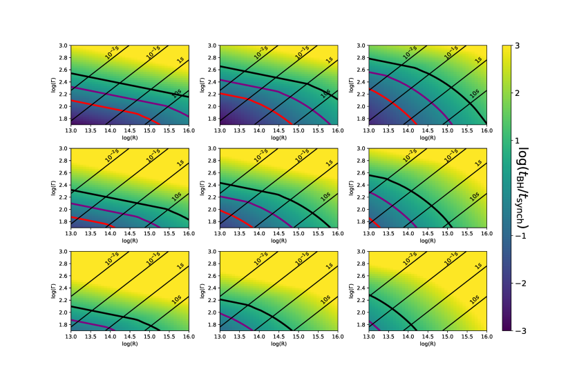
Figure 1: Comparison of cooling rate between the BeHe and synchrotron processes at $\gamma_{\rm p,m}$. From top to bottom the emitted luminosity is $10^{54}$, $10^{53}$ and $10^{52}$ erg s^-1, while from left to right the observed spectral peak frequency is $100$ keV, $300$ keV and 1 MeV. The purple, red and black thick lines correspond to $t_{\rm BeHe}=t_{\rm synch}$, $t_{\rm BeHe}=0.1t_{\rm synch}$, and $t_{\rm BeHe}=10t_{\rm synch}$ respectively. The thin black lines show the variability time expected from the Lorentz factor and radius $t_{\rm var}\sim r/(\Gamma^{2}c)$ for selected variability time $10^{-2}$s, $10^{-1}$s, $1$s and $10$s. The figure is made with $p=2.5$. A value of $p=3.5$ slightly increases the valid parameter space for proton synchrotron models by increasing the timescale ratio $t_{\rm BeHe}/t_{\rm synch}$ at small radii.

3 Spectral signature of Bethe-Heitler pairs

In this section, we obtain predictions for the comoving pair distribution and their emission spectrum in the case where the cooling via synchrotron and BeHe are comparable. In this situation, the proton distribution at $\gamma_{\rm p,m}$ is only marginally affected by BeHe cooling. This implies that the photon spectrum at the peak energy around 1 MeV (which is the optimal photon energy for BeHe pair creation; see Equation (4) and Appendix A) is not strongly modified by synchrotron radiation from the secondaries. If the secondary emission from the pairs do substantially contribute to the BeHe cooling of the protons, the BeHe pair creation becomes exponential in time and we are instead in the regime where BeHe dominates. Here, we use the proton synchrotron photons as targets to compute the rate at which pairs are created, namely in the case $t_{\rm BeHe}\raisebox{-1.29167pt}{\mbox{$\stackrel{{\scriptstyle>}}{{{}_{\sim}}}\,$}}t_{\rm synch}$.

A proton with Lorentz factor $\gamma_{\rm p}$ produces electrons and positrons with typical Lorentz factor $\gamma_{\pm}=\kappa_{\rm e}(m_{\rm p}/m_{\rm e})\gamma_{p}$, where $\kappa_{\rm e}$ is the inelasticity. The dependence of the inelasticity on $\gamma_{\rm p}x$, where $x$ is the target photon energy in units of electron rest mass, can be found in Mastichiadis et al. (2005). For photons at the peak energy, $\gamma_{\rm p}x$ is given by Equation (4) and is of the order of a few to a few hundreds. Looking at Figure 1 of Mastichiadis et al. (2005) for those values of $\gamma_{\rm p}x$, the inelasticity is found to vary between $10^{-3}$ and $10^{-4}$, giving an average pair Lorentz factor between $\gamma_{\pm}\sim 2\gamma_{\rm p}$ and $\gamma_{\pm}\sim\gamma_{\rm p}/5$. Considering that most of the protons have Lorentz factor $\gamma_{\rm p,m}\sim\gamma_{\rm p,c}$, we consider that all pairs are created with Lorentz factor $\gamma_{\pm,{\rm m}}\equiv\kappa_{\rm e}(m_{\rm p}/m_{\rm e})\gamma_{\rm p,m}$. In other words, we neglect the contribution of higher energy protons in the creation of pairs with higher energies. This effect only changes the very high energy photon spectrum, which is likely to be absorbed by pair creation. In addition, since the pairs are fast cooling, which follows as the protons are marginally fast cooling, they obtain a Lorentz factor much smaller than their initial Lorentz factor in one dynamical timescale $\gamma_{\pm,c}\ll\gamma_{\pm,{\rm m}}$, and therefore the exact details of their injection is lost via their cooling.

The pair production rate by BeHe is given by Chodorowski et al. (1992), but cannot be analytically integrated for a general photon spectrum. Analytical estimates in some specific cases were provided by Petropoulou & Mastichiadis (2015). We provide the integral expression used in our numerical computation in Appendix B. In order to get analytical estimates of the number of pairs, we write the ratio between the synchrotron power and BeHe power to be equal to the ratio of their timescales:

$$\frac{P_{\rm BeHe}^{\rm tot}}{N_{\rm p}P_{\rm synch}}=\left(\frac{t_{\rm BeHe}}{t_{\rm synch}}\right)^{-1},$$ (11)

where $P_{\rm BeHe}^{\rm tot}$ it the power emitted by all BeHe pairs. Using $P_{\rm BeHe}^{\rm tot}=\gamma_{\pm,{\rm m}}m_{\rm e}c^{2}\dot{n}_{\pm}V$, which is valid since the pairs are fast cooled, one obtains

$$\dot{n}_{\pm}=n_{\rm p}\left(\frac{t_{\rm BeHe}}{t_{\rm synch}}\right)^{-1}\frac{P_{\rm synch}}{\gamma_{\pm,{\rm m}}m_{\rm e}c^{2}}=\left\{\begin{aligned} &4.6\times 10^{8}~{}{\rm cm}^{-3}{\rm s}^{-1}~{}L_{52}^{2}\Gamma_{2}^{-\frac{4}{3}}r_{14}^{-\frac{40}{9}}\kappa_{\rm e,-4}^{-1}\nu_{\rm MeV}^{-\frac{20}{9}}&~{}~{}~{}~{}~{}&2x_{\rm m}\gamma_{\rm p,m}>\kappa_{0},\\ &9.2\times 10^{9}~{}{\rm cm}^{-3}{\rm s}^{-1}~{}L_{52}^{2}\nu_{\rm MeV}^{\frac{5}{12}}\Gamma_{2}^{-\frac{9}{2}}r_{14}^{-\frac{47}{12}}\kappa_{\rm e,-4}^{-1}&~{}~{}~{}~{}~{}&{\rm else.}\end{aligned}\right.$$ (12)

We note the very strong dependence on the parameters, specifically the radius and the peak energy. This means that in principle both scenarios with high and low pair yield are possible.

Assuming that all pairs are produced at Lorentz factor $\gamma_{\pm,{\rm m}}$ and that pair annihilation is negligible (see Section 4), the continuity equation for the pairs can be solved to obtain the pair distribution. This computation is done in Appendix C, and gives

$$n_{\pm}(\gamma_{\rm e})=\frac{m_{\rm e}c^{2}\dot{n}_{\pm}}{P_{\rm e}(\gamma_{\pm,{\rm m}})}\left(\frac{\gamma_{\pm,{\rm m}}}{\gamma_{\rm e}}\right)^{2}H(\gamma_{\pm,{\rm m}}-\gamma_{\rm e}),$$ (13)

namely a single power-law with index $-2$ extending from $\gamma_{\pm,{\rm m}}$ down to $\gamma\sim 1$. Here, $P_{\rm e}$ is the synchrotron power emitted by an electron and $H$ is the Heaviside function. We note that at low energies the pair distribution should substantially deviate from this power-law because of strong synchrotron self-absorption heating and pair annihilation. Our analysis also neglects the electrons originally present in the flow (see the discussion in Section 4).

We now estimate the emerging spectrum. The emitted synchrotron spectrum from the pair distribution in Equation (13) is a fast cooling power-law with $F_{\nu}\propto\nu^{-1/2}$. It extends from an observed peak frequency of

$$\nu_{{\rm m},\pm}=\left(\frac{\gamma_{\pm,{\rm m}}}{\gamma_{\rm p,m}}\right)^{2}\left(\frac{m_{\rm p}}{m_{\rm e}}\right)\nu^{\rm obs}=61.9~{}{\rm MeV}~{}\kappa_{\rm e,-4}^{2}\nu_{\rm MeV}$$ (14)

down to sub-keV energies. The synchrotron frequency of the pairs linearly depends on the observed peak frequency. It also indirectly depends on the other model parameters via the value of the inelasticity. Larger values of $\kappa_{\rm e}$ results from smaller values of $\gamma_{\rm p,m}\nu_{\rm m}$, i.e., larger Lorentz factor and peak frequency, and/or smaller radius and luminosity, see Equation (4). The shape of the spectrum above $\nu_{\pm,{\rm m}}$ depends on the shape of the proton distribution function and of the pair injection details. Since we are only giving analytical estimates, it is out of the scope of this paper to account for a detailed analysis at those energies. We note however that emission at GeV and eventually TeV energies are constrained by the LAT instrument on-board Fermi (e.g. Guetta et al. (2011)). The normalization of the spectrum is either obtained from the pair distribution function in Equation (13), or by considering the ratio of the synchrotron power to the BeHe power in Equation (11). Indeed, the value and parameter dependence of the ratio between the proton synchrotron peak and the BeHe peak, $\nu_{\rm m}F_{\nu_{\rm m}}/\nu_{\pm,{\rm m}}F_{\nu_{\pm,{\rm m}}}$, are well described by the ratio of the timescales given in Equation (10). This is true as long as $t_{\rm synch}$ is not much larger than $t_{\rm BeHe}$, so that the target photons for the BeHe process are those produced by proton synchrotron.

Figure 2 shows an example spectrum when the two timescales are comparable. A subdominant power-law extends from $\sim 100$ MeV all across the observation window. This extra component is solely due to synchrotron radiation from the BeHe pairs and it is simultaneous to the main MeV emission. It is potentially detectable at low energy (few tens of keV) and in the LLE data. In making this figure, we assumed $r_{14}=1$, $\Gamma_{2}=1$, $\nu_{\rm MeV}=1$, $L_{52}=10$, $\xi=1$ and $p=2.5$ (left) or $p=3.5$ (right). They both correspond to $t_{\rm BeHe}/t_{\rm synch}\sim 1.9$ (the approximate expression in Equation (10) gives $t_{\rm BeHe}/t_{\rm synch}\sim 0.85$). The figure was made with BeHe inelasticity $\kappa_{\rm e}\sim 10^{-4}$ to determine $\nu_{{\rm m},\pm}$. This value of $\kappa_{\rm e}$ is appropriate when $\gamma_{\rm p,m}h\nu_{\rm m}/(m_{\rm e}c^{2})\sim 100$, as obtained for this choice of parameters. The total number of pairs was calculated using the integral formulation of Chodorowski et al. (1992) (see Appendix B).

In this example, the overall synchrotron spectrum is strongly modified at low and high energies by an extra power-law produced by the synchrotron emission of the BeHe pairs. This is a clear spectral signature of the proton synchrotron emission model, which can help to differentiate proton synchrotron models from electron synchrotron models. Several properties of this power-law are well determined and weakly sensitive to the parameter of the model. First, its slope is set to be $\alpha=-1.5$ since it is produced by electrons and positrons in the fast cooling regime. Second, it extends from low (sub-keV) energy to high energy with a peak at few tens or hundreds of MeV. Therefore, this component crosses the entire GBM energy window. Third, the maximum energy of this component is linearly correlated with the peak frequency of the MeV component, as shown by Equation (14). Finally, the intensity of this component does not have a strong dependence on the uncertain value of the proton index $p$, but strongly depends on the luminosity, Lorentz factor and emission radius. The combination of all those characteristics provides a clear smoking-gun of proton synchrotron model.

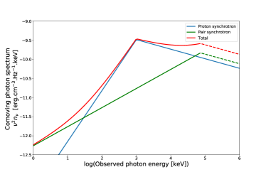
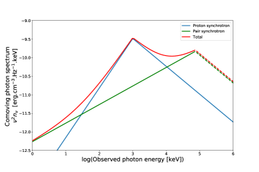
Figure 2: Photon spectrum in marginally dominant synchrotron cooling regime with $t_{\rm synch}\sim t_{\rm BeHe}$. Parameters are $r_{14}=1$, $\Gamma_{2}=1$, $\nu_{\rm MeV}=1$, $L_{52}=10$, $\xi=1$ and $p=2.5$ (left) or $p=3.5$ (right). Blue - proton synchrotron component. Green - BeHe synchrotron component. Red - total. It is clear that the emission from the secondary BeHe pairs greatly affect the overall shape of the spectrum at low ($\lesssim 30$ keV) and high ($\gtrsim 10$ MeV) energies . The frequency of the second peak is independent on the power-law index. Above the photon peak at $\sim 100~{}$MeV, the photon spectrum is not specified by our analysis as it depends on the details of the pair injection spectrum, and as such on the exact shape of the proton distribution function above $\gamma_{\rm p,m}$. This is represented by a dashed line.

4 Discussion and conclusion

Proton synchrotron models are an attractive solution to explain marginally fast cooling spectra from GRBs (Ghisellini et al., 2020). We have performed a detailed investigation of the effect of BeHe cooling on the protons and of the subsequent radiation of the BeHe pairs. For high bulk Lorentz factor $\Gamma$, large radius $r$ and low luminosity $L^{\rm obs}$, proton synchrotron emission dominates and no BeHe pair signature is expected. Conversely, synchrotron emission from the BeHe pairs dominates when the luminosity is high, and $\Gamma$ and $r$ are relatively low. This constitutes an additional test for the model: if no pair signature is observed in high luminosity bursts, large radii and high Lorentz factors are necessary. The magnetic luminosity is given by

$$L_{\rm B}=\pi cr^{2}\Gamma^{2}\frac{B^{2}}{8\pi}=4.43\times 10^{53}{\rm erg}~{}{\rm s}^{-1}r_{14}^{\frac{8}{3}}\xi^{\frac{4}{3}}t_{\rm v}^{-2}\nu_{\rm MeV}^{-\frac{2}{3}}$$ (15)

where we have replaced the Lorentz factor $\Gamma$ by the variability time $t_{\rm v}=r/(c\Gamma^{2})$ normalised to 1s. The large dependence on the radius and variability time implies a very large magnetic luminosity if no BeHe pair signature is observed. For instance, for a variability timescale of the order a few seconds as observed in the burst sample of Burgess et al. (2020), an observed luminosity of $L^{\rm obs}=10^{54}~{}$erg s^-1 requires that $r\sim 10^{15}$ cm to suppress the BeHe pair creation (see Figure 1). Using Equation (15), this implies a magnetic luminosity of a few $10^{56}$ erg s^-1. Such a high magnetic luminosity suggests that the jet is magnetically dominated, leading to an acceleration rate with $\Gamma\propto r^{1/3}$ (Drenkhahn & Spruit, 2002; Bégué et al., 2017), and possibly magnetic reconnection as the energy dissipation mechanism, see e.g. Lyutikov & Blackman (2001); Giannios & Uzdensky (2019).

In between the two regimes outlined above, we expect a parameter space where both signatures can be observed simultaneously in the MeV band (see Figure 2). This component might have already been observed in several GRBs. Indeed, it is reminiscent of the population of bursts whose spectra seems to have two components: a main emission peak together with a subdominant component well approximated by a power-law observed from a few keV to several tens of MeV (Ackermann et al., 2010; Guiriec et al., 2015). This sub-dominant power-law can be interpreted as the radiation from BeHe pairs, identified in our work as the spectral signature of proton synchrotron models.

Most notably, the spectra of GRB 190114C detected by MAGIC (MAGIC Collaboration et al., 2019) are composed of two components in the energy range 1keV - 1 GeV, with low energy slopes seemingly compatible with slow $\alpha=-2/3$ and fast $\alpha=-3/2$ cooling synchrotron radiation in some time bins (Chand et al. (2020), however see Ajello et al. (2020)). In addition, a spectral cut-off component at energies between $50$ to $100$ MeV was reported in Chand et al. (2020). We speculate that this burst might possess the clear signature of proton synchrotron with BeHe cooling discussed in this paper: 1) one main peak produced by proton synchrotron in the slow cooling regime, 2) a second component compatible with fast cooling synchrotron radiation from BeHe pairs and 3) a cutoff between $50$–$100$ MeV corresponding to the injection limit of BeHe pairs. Furthermore, analysis of panel c) and d) in Figure 2 of Chand et al. (2020) shows that the ratio between the low and the high peak frequency is about $100$, in rough agreement with Equation (14).

In our analysis, there are additional emission processes not dealt with that might modify the spectrum. We briefly discuss some of them here. First, we neglected the modification of the high energy peak by $\gamma\gamma$ absorption. Indeed, Equation (14) shows that the synchrotron peak of the pairs is marginally below the energy threshold for pair creation. Therefore, only the spectrum at energies larger than the peak can be affected by this process. Pair recombination could produce an observable characteristic around observed frequency $\nu_{{\rm obs},\gamma\gamma}\sim 2\Gamma\,m_{e}c^{2}/h=2.4\times 10^{22}~{}{\rm Hz}~{}\Gamma_{2}$. Yet, the time for pair recombination approximated by $t_{e^{\pm}\rightarrow\gamma\gamma}=2/(\sigma_{\rm T}n_{\pm}\langle v\rangle)$ is such that

$$\frac{t_{e^{\pm}\rightarrow\gamma\gamma}}{t_{\rm dyn}}=2.0\times 10^{2}~{}\Gamma_{2}^{\frac{10}{3}}r_{14}^{\frac{22}{9}}\kappa_{\rm e,-4}\nu_{\rm MeV}^{\frac{20}{9}}L_{52}^{-2},$$ (16)

where we have approximated the density of pairs as $n_{\pm}=\dot{n}_{\pm}t_{\rm dyn}$ using the upper branch of Equation (12) and use for the average electron velocity $\langle v\rangle=c$. Thus, pairs do not substantially recombine for our fiducial parameters. However, we note the large dependence on the parameters, therefore, such a signature could in some parameter space regions be present.

Furthermore, we did not treat the radiation from the initial population of electrons. This was discussed in Ghisellini et al. (2020), who argued that under the assumption that the same number of protons and electrons are accelerated, the electrons would not be seen if they achieve the same injection spectrum as the protons since their luminosity would be a factor $m_{e}/m_{p}$ lower. If instead of similar injection spectrum, both electrons and protons carry the same energy, electrons would radiate their energy in the TeV band, which should trigger a leptonic cascade. In addition, thermalization of the background electrons via synchrotron self-absorption could also change the low energy spectrum. We expect this process to change the spectrum mostly in the optical band, therefore our conclusions would be largely unaffected as we have focused on the keV to GeV band.

We assumed that photo-pion interaction is inefficient in our model since the threshold for this process is not reached for the fiducial parameters, see Equation (4). However, it was argued by Florou et al. (2021) that cooling by photo-pion dominates cooling by the BeHe process. We show in Appendix D the additional conditions that the parameters should satisfy for BeHe cooling to dominate. We find that this holds true for a large set of parameters. Yet, if a substantial amount of energy is transferred from protons to charged pions by photo-hadronic interaction, the spectrum above the peak would be modified.

In a future work, we will compute a table model with SOPRANO, a code designed to simulate lepto-hadronic processes in optically thin environment (Gasparyan et al., 2022). There, we perform direct fits of a proton synchrotron model with BeHe pair production to GRB 190114C, in order to understand if the additional power-law and its cutoff are in agreement with the model presented here. The sample of bursts in Burgess et al. (2020) will also be studied, in order to constrain the parameters and further test the model.

To conclude, proton synchrotron models have a clear smoking-gun signature: the synchrotron radiation produced by the BeHe pairs. The emerging spectrum is composed of a main synchrotron peak produced by protons, and a power-law with index $\alpha=-1.5$ extending from sub-keV energies to few tens or hundreds of MeV. The peak frequency of this component is linearly linked to the frequency of the MeV peak frequency. Identification of this extra power-law in spectra will help to constrain the emission mechanism of GRB jets and their parameters.

Appendix A Approximation to the Bethe-Heitler cooling rate

The cooling rate for a proton of Lorentz factor $\gamma_{\rm p}$ is given in a simple form by Chodorowski et al. (1992):

$$-\frac{d\gamma_{\rm p}^{\rm BeHe}}{dt}=\alpha r_{0}^{2}c\frac{m_{\rm e}}{m_{\rm p}}\int_{2}^{\infty}d\kappa n_{x}\left(\frac{\kappa}{2\gamma_{\rm p}}\right)\frac{\phi(\kappa)}{\kappa^{2}},$$ (A1)

where $\alpha$ is the fine structure constant, $r_{0}$ the classical electron radius, $\kappa=2\gamma_{\rm p}x$ is the maximum energy for a photon with energy $x=h\nu/m_{e}c^{2}$ in the proton rest frame, and $\phi(\kappa)/\kappa^{2}$ is the energy loss rate of a single-energy proton with Lorentz factor $\gamma_{p}$ in an isotropic photon background. It is approximately given by Equations (3.14) and (3.18) of Chodorowski et al. (1992). The photon distribution $n_{x}$ is the photon number per energy in units electron rest mass. In Equation (A1), the photon distribution function is used at the value $\kappa/(2\gamma_{\rm p})$. It is given by (compare with Equation (8))

$$n_{x}(x)=\frac{u_{\nu_{\rm m}}}{hx}\left\{\begin{aligned} &\left(\frac{x}{x_{\rm c}}\right)^{1/3}\xi^{1/2}\quad&&x<x_{\rm c}\\ &\left(\frac{x}{x_{\rm m}}\right)^{-1/2}\quad&&x_{\rm c}<x<x_{\rm m}\\ &\left(\frac{x}{x_{\rm m}}\right)^{-p/2}\quad&&x>x_{\rm m}\end{aligned}\right.$$ (A2)

where $x_{\rm c}=h\nu_{c}/(m_{\rm e}c^{2})$ and $x_{\rm m}=h\nu_{\rm m}/m_{\rm e}c^{2}$ are the cooling and injection frequencies in units of the electron rest mass energy, $\xi=\nu_{c}/\nu_{m}$ and $u_{\nu_{m}}$ is the peak spectral energy density as given by Equation (7). In order to obtain analytical results that still factorize the photon spectrum, we approximate $\phi(\kappa)/\kappa^{2}$ by a $\delta$-function that is normalized to the integral between $2<\kappa<500$ (those numbers are arbitrarily, but we numerically checked that they encompass most of the cooling contribution):

$$\frac{\phi(\kappa)}{\kappa^{2}}=A_{\pm}\delta(\kappa-\kappa_{0})$$ (A3)

where we find $A_{\pm}=420$ and $\kappa_{0}=40$, roughly corresponding to the position of the maximum of $\phi(\kappa)/\kappa^{2}$. Using this approximation in Equation (A1) gives

$$-\frac{d\gamma_{\rm p}^{\rm BeHe}}{dt}\sim\alpha r_{0}^{2}c\frac{m_{\rm e}}{m_{\rm p}}A_{\pm}n_{x}\left(\frac{\kappa_{0}}{2\gamma_{\rm p}}\right)$$ (A4)

We now use the expression for the photon spectrum given in Equation (8) to obtain in marginally fast ($\xi>1$) cooling

$$-\frac{d\gamma_{\rm p}^{\rm BeHe}}{dt}= \alpha r_{0}^{2}c\frac{m_{\rm e}}{m_{\rm p}}\frac{A_{\pm}}{h}u_{\nu_{\rm m}}\left\{\begin{aligned} &\left(\frac{2\gamma_{\rm p}}{\kappa_{0}}\right)^{\frac{2}{3}}\left(\frac{1}{x_{\rm c}}\right)^{\frac{1}{3}}\xi^{\frac{1}{2}}&&\frac{\kappa_{0}}{2\gamma_{\rm p}}<x_{\rm c}\\ &\left(\frac{2\gamma_{\rm p}}{\kappa_{0}}\right)^{\frac{3}{2}}\left(\frac{1}{x_{\rm m}}\right)^{-\frac{1}{2}}&&x_{\rm c}<\frac{\kappa_{0}}{2\gamma_{\rm p}}<x_{\rm m}\\ &\left(\frac{2\gamma_{\rm p}}{\kappa_{0}}\right)^{1+\frac{p}{2}}\left(\frac{1}{x_{\rm m}}\right)^{-\frac{p}{2}}&&x_{\rm m}<\frac{\kappa_{0}}{2\gamma_{\rm p}}\end{aligned}\right.$$ (A5)

The cooling time by the BeHe process is finally obtained by

$$t_{\rm BeHe}^{-1}=\left|\frac{1}{\gamma_{\rm p}}\frac{d\gamma_{\rm p}^{\rm BeHe}}{dt}\right|$$ (A6)

Appendix B Bethe-Heitler pair production rate in marginally fast cooling

In this appendix, we seek an approximate expression for the pair production under the assumption of marginally fast cooling $\xi\equiv 1$. The pair production rate is given by Chodorowski et al. (1992)

$$\frac{\partial N_{\pm}}{\partial t}=c\frac{3}{8\pi}\frac{\sigma_{\rm T}\alpha}{\gamma_{\rm p}}\int_{2}^{\infty}n_{x}\left(\frac{\kappa}{2\gamma_{\rm p}}\right)\frac{\psi(\kappa)}{\kappa^{2}}d\kappa,$$ (B1)

where $\psi(\kappa)$ is given by Equations 2.3 of Chodorowski et al. (1992). Multiplying this equation by an electron energy $\gamma_{\pm}m_{e}c^{2}$ and integrating over electron energies corresponds to the cooling rate of a proton whose expression is given by Equation (A1). Replacing with the expression of the synchrotron spectrum in the marginally fast cooling scenario with $\gamma_{\rm m}=\gamma_{\rm c}$ gives:

$$\frac{8\pi\gamma_{\rm p}}{3c\sigma_{\rm T}\alpha}\frac{\partial N_{\pm}}{\partial t}=\int_{2}^{\kappa_{*}}n_{x}\left(\frac{\kappa}{2\gamma_{\rm p}}\right)\frac{\psi(\kappa)}{\kappa^{2}}d\kappa+\int_{\kappa_{*}}^{\infty}n_{x}\left(\frac{\kappa}{2\gamma_{\rm p}}\right)\frac{\psi(\kappa)}{\kappa^{2}}d\kappa$$ (B2)

where $\kappa_{*}\geq 2$ is such that

$$\frac{\kappa_{*}}{2\gamma_{\rm p}}=\frac{h\nu_{\rm m}}{m_{\rm e}c^{2}}$$ (B3)

is the energy of a photon at the spectral peak in the rest frame of the proton. Using the expression for the photon spectrum given by Equation (8), it becomes:

$$\frac{8\pi\gamma_{\rm p}}{3c\sigma_{\rm T}\alpha}\frac{\partial N_{\pm}}{\partial t} =\frac{2\gamma_{\rm p}}{h}\left(\frac{1}{2\gamma_{\rm p}x_{\rm m}}\right)^{\frac{1}{3}}u_{\nu_{\rm m}}\int_{2}^{\kappa_{*}}\kappa^{-\frac{2}{3}}\frac{\psi(\kappa)}{\kappa^{2}}d\kappa+\frac{2\gamma_{\rm p}}{h}\left(\frac{1}{2\gamma_{\rm p}x_{\rm m}}\right)^{-\frac{p}{2}}u_{\nu_{\rm m}}\int_{\kappa_{*}}^{\infty}\kappa^{-\frac{p_{\rm e}}{2}-1}\frac{\psi(\kappa)}{\kappa^{2}}d\kappa$$ (B4)

Appendix C Electron spectrum for $\delta-$function injection with synchrotron cooling

We assume that electron-positron pairs are produced with a single Lorentz factor $\gamma_{\pm,{\rm m}}$ and we proceed by solving the kinetic equation describing the evolution of the pair distribution function

$$\frac{\partial n_{\pm}}{\partial t}+\frac{1}{m_{\rm e}c^{2}}\frac{\partial}{\partial\gamma_{\rm e}}\left(P_{\rm e}(\gamma)n_{\pm}\right)=\dot{n}_{\pm}\delta(\gamma-\gamma_{\pm,{\rm m}})$$ (C1)

where the pair distribution function $n_{\pm}(\gamma_{\rm e},t)$ is a function of both time and electron energy, and $\dot{n}_{\pm}$ is the pair production rate by the BeHe process, given by Equation (13). Let $\epsilon$ be a small positive variable and let us integrate the above equation between $\gamma_{\pm,{\rm m}}-\epsilon$ and $\gamma_{\pm,{\rm m}}+\epsilon$. Keeping only the zeroth order term in $\epsilon$, we obtain

$$\frac{1}{m_{\rm e}c^{2}}\left[P_{\rm e}n_{\pm}\right]_{\gamma_{\pm,{\rm m}}-\epsilon}^{\gamma_{\pm,{\rm m}}+\epsilon}=\dot{n}_{\pm}$$ (C2)

describing a jump in the solution at $\gamma_{\pm,{\rm m}}$. Since particles are cooling, $n_{\pm}$ is null for $\gamma>\gamma_{\pm,{\rm m}}$. We now solve the equation for $\gamma<\gamma_{\pm,{\rm m}}$. Further assuming that electron are fast cool, far from $\gamma_{\pm,\rm c}\ll\gamma_{\pm,{\rm m}}$, the equation can be further simplified to

$$\frac{\partial}{\partial\gamma}\left(P_{\rm e}n_{\pm}\right)=0$$ (C3)

Therefore, the solution is of the form

$$n_{\pm}=Q\times\left(\frac{\gamma_{\pm,{\rm m}}}{\gamma}\right)^{2}$$ (C4)

where we introduced $\gamma_{\pm,{\rm m}}$ for convenience. We use Equation (C2) to obtain

$$Q=\frac{m_{\rm e}c^{2}}{P_{\rm e}(\gamma_{\pm,{\rm m}})}\dot{n}_{\pm}$$ (C5)

Appendix D Photo-pion cooling of protons on proton synchrotron photons

The cooling of protons by photopion interaction is given by (Mannheim & Schlickeiser, 1994; Begelman et al., 1990; Waxman & Bahcall, 1997)

$$t_{\rm p\pi}^{-1}=\frac{c}{2\gamma_{\rm p}^{2}}\int_{\bar{\epsilon}_{\rm th}}^{\infty}d\bar{\epsilon}\sigma_{p\pi}(\bar{\epsilon})K_{p}(\bar{\epsilon})\bar{\epsilon}\int_{\frac{\bar{\epsilon}}{2\gamma_{\rm p}}}^{\infty}dx\frac{n_{x}(x)}{x^{2}}$$ (D1)

Following Petropoulou & Mastichiadis (2015), we set

$$\sigma_{\rm p\pi} =\sigma_{0}H(\bar{\epsilon}-\bar{\epsilon}_{\rm th})$$ (D2)

$$\sigma_{0} =1.5\times 10^{-4}\sigma_{\rm T}$$ (D3)

$$K_{\rm p} =0.2$$ (D4)

$$\bar{\epsilon}_{\rm th} =145{\rm~{}MeV}$$ (D5)

where $H$ is the Heaviside function. The cooling time becomes

$$t_{\rm p\pi}^{-1}=\frac{c}{2\gamma_{\rm p}^{2}}K_{p}\sigma_{0}\int_{\bar{\epsilon}_{\rm th}}^{\infty}d\bar{\epsilon}\bar{\epsilon}\int_{\frac{\bar{\epsilon}}{2\gamma_{\rm p}}}^{\infty}dx\frac{n(x)}{x^{2}},$$ (D6)

where $\bar{\epsilon}$ and $\bar{\epsilon}_{\rm th}$ are expressed in units of the electron rest mass energy.

Using the photon distribution function given by Equation (A2), assuming $x_{m}=x_{c}$ and $2\gamma_{\rm p}x_{m}>\bar{\epsilon}_{\rm th}$, we obtain

$$\frac{t_{\rm p\pi}^{-1}}{\frac{c}{2\gamma_{\rm p}^{2}}K_{p}\sigma_{0}}= \int_{\bar{\epsilon}_{\rm th}}^{2\gamma_{p}x_{m}}d\bar{\epsilon}\bar{\epsilon}\left[\int_{\frac{\bar{\epsilon}}{2\gamma_{\rm p}}}^{x_{m}}dx\frac{1}{x^{2}}\frac{1}{h}\frac{1}{x}u_{\nu_{m}}\left(\frac{x}{x_{m}}\right)^{\frac{1}{3}}+\int_{x_{m}}^{\infty}dx\frac{1}{x^{2}}\frac{1}{h}\frac{1}{x}u_{\nu_{m}}\left(\frac{x}{x_{m}}\right)^{-\frac{p}{2}}\right]$$ (D7)

$$+ \int_{2\gamma_{p}x_{m}}^{\infty}d\bar{\epsilon}\bar{\epsilon}\int_{\frac{\bar{\epsilon}}{2\gamma_{\rm p}}}^{\infty}dx\frac{1}{x^{2}}\frac{1}{h}\frac{1}{x}u_{\nu_{m}}\left(\frac{x}{x_{m}}\right)^{-\frac{p}{2}}$$

After some algebra, it simplifies to

$$\frac{t_{\rm p\pi}^{-1}}{\frac{c}{2\gamma_{\rm p}^{2}}K_{p}\sigma_{0}\frac{u_{\nu_{m}}}{h}}=\left\{\begin{aligned} &\frac{(2\gamma_{p})^{2}}{(2+\frac{p}{2})\frac{p}{2}}&~{}~{}~{}~{}~{}~{}~{}&2\gamma_{p}x_{m}\rightarrow\bar{\epsilon}_{\rm th}^{+}\\ &(2\gamma_{p})^{2}\left[\frac{9}{5}+\left(\frac{1}{(2+\frac{p}{2})}-\frac{1}{(5/3)}\right)\frac{1}{2}+\frac{1}{(2+\frac{p}{2})\frac{p}{2}}\right]&&2\gamma_{p}x_{m}\gg\bar{\epsilon}_{\rm th}\end{aligned}\right.$$ (D8)

where the dependence on the energy $x_{m}$ simplifies with the normalisation of the photon spectrum. If $2\gamma_{p}x_{m}<\bar{\epsilon}_{\rm th}$, the cooling time is simplified as

$$\frac{t_{\rm p\pi}^{-1}}{\frac{c}{2\gamma_{\rm p}^{2}}K_{p}\sigma_{0}\frac{u_{\nu_{m}}}{h}}= \left(\frac{x_{m}}{\bar{\epsilon}_{\rm th}}\right)^{\frac{p}{2}}\frac{(2\gamma_{p})^{2+\frac{p}{2}}}{\left(2+\frac{p}{2}\right)\frac{p}{2}}$$ (D9)

To compare BeHe and photopion cooling, only three cases needs to be considered : they depend on the location of $2\gamma_{p}x_{m}$ with respect to $\kappa_{0}$ and $\bar{\epsilon}_{\rm th}$. The condition $2x_{m}\gamma_{\rm p,m}>\bar{\epsilon}_{\rm th}>\kappa_{0}$ is rarely satisfied. If it is, photo-pion cooling dominates by large over BeHe cooling. For $\kappa_{0}<2\gamma_{\rm p}x_{\rm m}<\bar{\epsilon}_{\rm th}$, the ratio of cooling time is simplified to

$$\frac{t_{\rm BeHe}^{-1}}{t_{\rm p\pi}^{-1}}=\left(2+\frac{p}{2}\right)\frac{p}{2}\frac{A_{\pm}}{K_{p}}\frac{\bar{\epsilon}_{\rm th}^{\frac{p}{2}}}{\kappa_{0}^{\frac{2}{3}}}\frac{\alpha r_{0}^{2}\frac{m_{\rm e}}{m_{\rm p}}}{\sigma_{0}}\frac{1}{x_{m}^{\frac{p}{2}+\frac{1}{3}}(2\gamma_{p})^{\frac{p}{2}+\frac{1}{3}}}=0.39\Gamma_{2}^{p+\frac{2}{3}}\nu_{1MeV}^{-\frac{5p}{6}-\frac{5}{9}}R_{14}^{-\frac{p}{6}-\frac{1}{9}}$$ (D10)

where we set $\nu_{c}=\nu_{m}$ (i.e. $\xi=1$). For the computation of the numerical factor, we set $p=2.5$. In that case, photo-pion cooling dominates over BeHe, but we point the strong dependence on the Lorentz factor $\Gamma$. For $\Gamma_{2}=3$, the cooling is dominated by BeHe. In the case $\bar{\epsilon}_{\rm th}>\kappa_{0}>2\gamma_{\rm p}x_{\rm m}$, it comes

$$\frac{t_{\rm BeHe}^{-1}}{t_{\rm p\pi}^{-1}} =\left(2+\frac{p}{2}\right)\frac{p}{2}\frac{A_{\pm}}{K_{p}}\frac{\bar{\epsilon}_{\rm th}^{\frac{p}{2}}}{\kappa_{0}^{1+\frac{p}{2}}}\frac{\alpha r_{0}^{2}\frac{m_{\rm e}}{m_{\rm p}}}{\sigma_{0}}\sim 7.7,$$ (D11)

which is independent on $\gamma_{p}$ and on $x_{m}$, and therefore remains constant for any parameters of the problem. In this numerical estimate, we set $p=2.5$.

References

- Aartsen et al. (2017) Aartsen, M., Ackermann, M., Adams, J., et al. 2017, ApJ, 843, 112A
- Ackermann et al. (2010) Ackermann, M., Asano, K., Atwood, W. B., et al. 2010, ApJ, 716, 1178, doi: 10.1088/0004-637X/716/2/1178
- Acuner et al. (2020) Acuner, Z., Ryde, F., Pe’er, A., Mortlock, D., & Ahlgren, B. 2020, ApJ, 893, 128, doi: 10.3847/1538-4357/ab80c7
- Ahlgren et al. (2015) Ahlgren, B., Larsson, J., Nymark, T., Ryde, F., & Pe’er, A. 2015, MNRAS, 454, L31, doi: 10.1093/mnrasl/slv114
- Ajello et al. (2020) Ajello, M., Arimoto, M., Axelsson, M., et al. 2020, ApJ, 890, 9, doi: 10.3847/1538-4357/ab5b05
- Albert et al. (2017) Albert, A., André, M., Anghinolfi, M., et al. 2017, MNRAS, 469, 906, doi: 10.1093/mnras/stx902
- Asano et al. (2009) Asano, K., Inoue, S., & Mészáros, P. 2009, ApJ, 699, 953, doi: 10.1088/0004-637X/699/2/953
- Axelsson & Borgonovo (2015) Axelsson, M., & Borgonovo, L. 2015, MNRAS, 447, 3150, doi: 10.1093/mnras/stu2675
- Band et al. (1993) Band, D., Matteson, J., Ford, L., et al. 1993, ApJ, 413, 281, doi: 10.1086/172995
- Bednarz & Ostrowski (1998) Bednarz, J., & Ostrowski, M. 1998, Phys. Rev. Lett., 80, 3911, doi: 10.1103/PhysRevLett.80.3911
- Begelman et al. (1990) Begelman, M. C., Rudak, B., & Sikora, M. 1990, ApJ, 362, 38, doi: 10.1086/169241
- Bégué et al. (2017) Bégué, D., Pe’er, A., & Lyubarsky, Y. 2017, MNRAS, 467, 2594, doi: 10.1093/mnras/stx237
- Bégué et al. (2013) Bégué, D., Siutsou, I. A., & Vereshchagin, G. V. 2013, ApJ, 767, 139, doi: 10.1088/0004-637X/767/2/139
- Bégué & Vereshchagin (2014) Bégué, D., & Vereshchagin, G. V. 2014, MNRAS, 439, 924, doi: 10.1093/mnras/stu011
- Beloborodov (2010) Beloborodov, A. M. 2010, MNRAS, 407, 1033, doi: 10.1111/j.1365-2966.2010.16770.x
- Beniamini et al. (2018) Beniamini, P., Barniol Duran, R., & Giannios, D. 2018, MNRAS, 476, 1785, doi: 10.1093/mnras/sty340
- Böttcher & Dermer (1998) Böttcher, M., & Dermer, C. D. 1998, ApJ, 499, L131, doi: 10.1086/311366
- Bošnjak et al. (2009) Bošnjak, Ž., Daigne, F., & Dubus, G. 2009, A&A, 498, 677, doi: 10.1051/0004-6361/200811375
- Burgess (2019) Burgess, J. M. 2019, A&A, 629, A69, doi: 10.1051/0004-6361/201935140
- Burgess et al. (2020) Burgess, J. M., Bégué, D., Greiner, J., et al. 2020, Nature Astronomy, 4, 174, doi: 10.1038/s41550-019-0911-z
- Chand et al. (2020) Chand, V., Pal, P. S., Banerjee, A., et al. 2020, ApJ, 903, 9, doi: 10.3847/1538-4357/abb5fc
- Chodorowski et al. (1992) Chodorowski, M. J., Zdziarski, A. A., & Sikora, M. 1992, ApJ, 400, 181, doi: 10.1086/171984
- Comisso et al. (2020) Comisso, L., Sobacchi, E., & Sironi, L. 2020, ApJ, 895, L40, doi: 10.3847/2041-8213/ab93dc
- Crumley et al. (2019) Crumley, P., Caprioli, D., Markoff, S., & Spitkovsky, A. 2019, MNRAS, 485, 5105, doi: 10.1093/mnras/stz232
- Crumley & Kumar (2013) Crumley, P., & Kumar, P. 2013, MNRAS, 429, 3238, doi: 10.1093/mnras/sts581
- Daigne et al. (2011) Daigne, F., Bošnjak, Ž., & Dubus, G. 2011, A&A, 526, A110, doi: 10.1051/0004-6361/201015457
- Daigne & Mochkovitch (1998) Daigne, F., & Mochkovitch, R. 1998, MNRAS, 296, 275, doi: 10.1046/j.1365-8711.1998.01305.x
- Dereli-Bégué et al. (2020) Dereli-Bégué, H., Pe’er, A., & Ryde, F. 2020, ApJ, 897, 145, doi: 10.3847/1538-4357/ab9a2d
- Drenkhahn & Spruit (2002) Drenkhahn, G., & Spruit, H. C. 2002, A&A, 391, 1141, doi: 10.1051/0004-6361:20020839
- Florou et al. (2021) Florou, I., Petropoulou, M., & Mastichiadis, A. 2021, MNRAS, doi: 10.1093/mnras/stab1285
- Gasparyan et al. (2022) Gasparyan, S., Bégué, D., & Sahakyan, N. 2022, MNRAS, 509, 2102, doi: 10.1093/mnras/stab2688
- Ghisellini et al. (2020) Ghisellini, G., Ghirlanda, G., Oganesyan, G., et al. 2020, A&A, 636, A82, doi: 10.1051/0004-6361/201937244
- Giannios (2006) Giannios, D. 2006, A&A, 457, 763, doi: 10.1051/0004-6361:20065000
- Giannios & Uzdensky (2019) Giannios, D., & Uzdensky, D. A. 2019, MNRAS, 484, 1378, doi: 10.1093/mnras/stz082
- Goodman (1986) Goodman, J. 1986, ApJ, 308, L47, doi: 10.1086/184741
- Guetta et al. (2011) Guetta, D., Pian, E., & Waxman, E. 2011, A&A, 525, A53, doi: 10.1051/0004-6361/201014344
- Guiriec et al. (2015) Guiriec, S., Kouveliotou, C., Daigne, F., et al. 2015, ApJ, 807, 148, doi: 10.1088/0004-637X/807/2/148
- Gupta & Zhang (2007) Gupta, N., & Zhang, B. 2007, MNRAS, 380, 78, doi: 10.1111/j.1365-2966.2007.12051.x
- Hümmer et al. (2010) Hümmer, S., Rüger, M., Spanier, F., & Winter, W. 2010, ApJ, 721, 630, doi: 10.1088/0004-637X/721/1/630
- Kirk et al. (2000) Kirk, J. G., Guthmann, A. W., Gallant, Y. A., & Achterberg, A. 2000, ApJ, 542, 235, doi: 10.1086/309533
- Li (2019) Li, L. 2019, ApJS, 242, 16, doi: 10.3847/1538-4365/ab1b78
- Lipari et al. (2007) Lipari, P., Lusignoli, M., & Meloni, D. 2007, Phys. Rev. D, 75, 123005, doi: 10.1103/PhysRevD.75.123005
- Lundman et al. (2013) Lundman, C., Pe’er, A., & Ryde, F. 2013, MNRAS, 428, 2430, doi: 10.1093/mnras/sts219
- Lyutikov & Blackman (2001) Lyutikov, M., & Blackman, E. G. 2001, MNRAS, 321, 177, doi: 10.1046/j.1365-8711.2001.04190.x
- MAGIC Collaboration et al. (2019) MAGIC Collaboration, Acciari, V. A., Ansoldi, S., et al. 2019, Nature, 575, 455, doi: 10.1038/s41586-019-1750-x
- Mannheim & Schlickeiser (1994) Mannheim, K., & Schlickeiser, R. 1994, A&A, 286, 983. https://arxiv.org/abs/astro-ph/9402042
- Mastichiadis et al. (2005) Mastichiadis, A., Protheroe, R. J., & Kirk, J. G. 2005, A&A, 433, 765, doi: 10.1051/0004-6361:20042161
- Mészáros & Rees (2000) Mészáros, P., & Rees, M. J. 2000, ApJ, 530, 292, doi: 10.1086/308371
- Mücke et al. (2000) Mücke, A., Engel, R., Rachen, J. P., Protheroe, R. J., & Stanev, T. 2000, Computer Physics Communications, 124, 290, doi: 10.1016/S0010-4655(99)00446-4
- Nakar et al. (2009) Nakar, E., Ando, S., & Sari, R. 2009, ApJ, 703, 675, doi: 10.1088/0004-637X/703/1/675
- Narayan & Kumar (2009) Narayan, R., & Kumar, P. 2009, MNRAS, 394, L117, doi: 10.1111/j.1745-3933.2009.00624.x
- Oganesyan et al. (2018) Oganesyan, G., Nava, L., Ghirlanda, G., & Celotti, A. 2018, A&A, 616, A138, doi: 10.1051/0004-6361/201732172
- Oganesyan et al. (2019) Oganesyan, G., Nava, L., Ghirlanda, G., Melandri, A., & Celotti, A. 2019, A&A, 628, A59, doi: 10.1051/0004-6361/201935766
- Paczynski (1986) Paczynski, B. 1986, ApJ, 308, L43, doi: 10.1086/184740
- Parsotan & Lazzati (2018) Parsotan, T., & Lazzati, D. 2018, ApJ, 853, 8, doi: 10.3847/1538-4357/aaa087
- Pe’er (2015) Pe’er, A. 2015, Advances in Astronomy, 2015, 907321, doi: 10.1155/2015/907321
- Pe’er & Ryde (2011) Pe’er, A., & Ryde, F. 2011, ApJ, 732, 49, doi: 10.1088/0004-637X/732/1/49
- Pe’er & Waxman (2005) Pe’er, A., & Waxman, E. 2005, ApJ, 628, 857, doi: 10.1086/431139
- Pe’Er et al. (2012) Pe’Er, A., Zhang, B.-B., Ryde, F., et al. 2012, MNRAS, 420, 468, doi: 10.1111/j.1365-2966.2011.20052.x
- Petropoulou (2014) Petropoulou, M. 2014, MNRAS, 442, 3026, doi: 10.1093/mnras/stu1079
- Petropoulou & Mastichiadis (2015) Petropoulou, M., & Mastichiadis, A. 2015, MNRAS, 447, 36, doi: 10.1093/mnras/stu2364
- Pitik et al. (2021) Pitik, T., Tamborra, I., & Petropoulou, M. 2021, J. Cosmology Astropart. Phys, 2021, 034, doi: 10.1088/1475-7516/2021/05/034
- Preece et al. (1998) Preece, R. D., Briggs, M. S., Mallozzi, R. S., et al. 1998, ApJ, 506, L23, doi: 10.1086/311644
- Razzaque et al. (2010) Razzaque, S., Dermer, C. D., & Finke, J. D. 2010, The Open Astronomy Journal, 3, 150, doi: 10.2174/1874381101003010150
- Rees & Meszaros (1994) Rees, M. J., & Meszaros, P. 1994, ApJ, 430, L93, doi: 10.1086/187446
- Ryde et al. (2017) Ryde, F., Lundman, C., & Acuner, Z. 2017, MNRAS, 472, 1897, doi: 10.1093/mnras/stx2019
- Ryde & Pe’er (2009) Ryde, F., & Pe’er, A. 2009, ApJ, 702, 1211, doi: 10.1088/0004-637X/702/2/1211
- Ryde et al. (2010) Ryde, F., Axelsson, M., Zhang, B. B., et al. 2010, ApJ, 709, L172, doi: 10.1088/2041-8205/709/2/L172
- Sahu & Fortín (2020) Sahu, S., & Fortín, C. E. L. 2020, ApJ, 895, L41, doi: 10.3847/2041-8213/ab93da
- Samuelsson et al. (2021) Samuelsson, F., Lundman, C., & Ryde, F. 2021, arXiv e-prints, arXiv:2111.01810. https://arxiv.org/abs/2111.01810
- Sari et al. (1996) Sari, R., Narayan, R., & Piran, T. 1996, ApJ, 473, 204, doi: 10.1086/178136
- Sari et al. (1998) Sari, R., Piran, T., & Narayan, R. 1998, ApJ, 497, L17, doi: 10.1086/311269
- Sironi et al. (2013) Sironi, L., Spitkovsky, A., & Arons, J. 2013, ApJ, 771, 54, doi: 10.1088/0004-637X/771/1/54
- Totani (1998) Totani, T. 1998, ApJ, 509, L81, doi: 10.1086/311772
- Uhm & Zhang (2014) Uhm, Z. L., & Zhang, B. 2014, Nature Physics, 10, 351, doi: 10.1038/nphys2932
- Vianello et al. (2018) Vianello, G., Gill, R., Granot, J., et al. 2018, ApJ, 864, 163, doi: 10.3847/1538-4357/aad6ea
- von Kienlin et al. (2020) von Kienlin, A., Meegan, C. A., Paciesas, W. S., et al. 2020, ApJ, 893, 46, doi: 10.3847/1538-4357/ab7a18
- Vurm & Beloborodov (2016) Vurm, I., & Beloborodov, A. M. 2016, ApJ, 831, 175, doi: 10.3847/0004-637X/831/2/175
- Waxman & Bahcall (1997) Waxman, E., & Bahcall, J. 1997, Phys. Rev. Lett., 78, 2292, doi: 10.1103/PhysRevLett.78.2292
- Yu et al. (2015) Yu, H.-F., van Eerten, H. J., Greiner, J., et al. 2015, A&A, 583, A129, doi: 10.1051/0004-6361/201527015
- Zhang & Yan (2011) Zhang, B., & Yan, H. 2011, ApJ, 726, 90, doi: 10.1088/0004-637X/726/2/90
- Zhang & Zhang (2014) Zhang, B., & Zhang, B. 2014, ApJ, 782, 92, doi: 10.1088/0004-637X/782/2/92
- Zhang et al. (2018) Zhang, B.-B., Zhang, B., Castro-Tirado, A. J., et al. 2018, Nature Astronomy, 2, 69, doi: 10.1038/s41550-017-0309-8