A machine learning approach to infer the accreted stellar mass fractions of central galaxies in the TNG100 simulation

Abstract

We propose a random forest (RF) machine learning approach to determine the accreted stellar mass fractions ($f_{\mathrm{acc}}$) of central galaxies, based on various dark matter halo and galaxy features. The RF is trained and tested using 2,710 galaxies with stellar mass $\log_{10}M_{\ast}/M_{\odot}>10.16$ from the TNG100 simulation. Galaxy size is the most important individual feature when calculated in 3-dimensions, which becomes less important after accounting for observational effects. For smaller galaxies, the rankings for features related to merger histories increase. When an entire set of halo and galaxy features are used, the prediction is almost unbiased, with root-mean-square error (RMSE) of $\sim$0.068. A combination of up to three features with different types (galaxy size, merger history and morphology) already saturates the power of prediction. If using observable features, the RMSE increases to $\sim$0.104, and a combined usage of stellar mass, galaxy size plus galaxy concentration achieves similar predictions. Lastly, when using galaxy density, velocity and velocity dispersion profiles as features, which approximately represent the maximum amount of information extracted from galaxy images and velocity maps, the prediction is not improved much. Hence the limiting precision of predicting $f_{\mathrm{acc}}$ is $\sim$0.1 with observables, and the multi-component decomposition of galaxy images should have similar or larger uncertainties. If the central black hole mass and the spin parameter of galaxies can be accurately measured in future observations, the RMSE is promising to be further decreased by $\sim$20%.

1 Introduction

In the structure formation paradigm of $\Lambda$CDM, galaxies form by the cooling and condensation of gas at centres of dark matter haloes (White & Rees, 1978). It is usually believed that galaxy formation involves two phases, an early rapid formation of “in-situ” stars through gas cooling and a later phase of mass growth of “ex-situ” stars through accretion of smaller satellite galaxies, which were originally central galaxies of smaller dark matter haloes. These smaller haloes and galaxies, after falling into larger haloes, become the so-called subhaloes and satellite galaxies. Satellites lose their stellar mass under tidal stripping. Stripped stellar materials build up the outskirts of central galaxies and are more metal poor than “in-situ” stars, which form the diffuse light or the extended stellar halo around the central galaxy (e.g. Bullock & Johnston, 2005).

Theoretical studies on the formation of extended stellar haloes involve a few different approaches, including analytical models (e.g. Purcell et al., 2007), hydrodynamical simulations (e.g. Oser et al., 2010; Lackner et al., 2012; Pillepich et al., 2014; Rodriguez-Gomez et al., 2016; Karademir et al., 2019) and semi-analytical approaches of particle painting/tagging method (e.g. Cooper et al., 2010). It is demonstrated that the fraction of accreted stellar mass with respect to the total mass of galaxies is higher for more massive galaxies and for elliptical galaxies. The maximum amount of intracluster component in the most massive dark matter haloes can be six times as large as the in-situ formed stellar mass of the central galaxy (e.g. Yang et al., 2009). In addition, Rodriguez-Gomez et al. (2016, 2017) also demonstrated the dependence of the fraction of ex-situ stars on other halo and galaxy properties in Illustris, such as the formation time, merger gas fraction, merger lookback time and merger mass ratio.

Observationally, the determination of accreted stellar mass fractions for galaxies often relies on a multi-component decomposition of galaxy images or surface brightness profiles (e.g. D’Souza et al., 2014; Oh et al., 2017). The inner and outer components of the best-fitting model profiles are usually assumed to represent the in-situ and ex-situ components. The decomposition also indicates on average larger fractions of ex-situ stars in more massive galaxies and in early-type galaxies (e.g D’Souza et al., 2014), in general agreement with predictions from numerical simulations.

However, the multi-component fitting to observed surface brightness profiles of galaxies might be subject to unknown systematic uncertainties. For example, Remus & Forbes (2021) tested multi-component decomposition using mock galaxy images. They reported that the best-fitting inner and outer components deviate from the true in-situ and ex-situ components. The fitting is in fact more difficult for late-type galaxies, which have rich substructures and breaks in their surface brightness profiles. As a result, D’Souza et al. (2014) adopted triple Sérsic models, with the approach of fitting and fixing the inner two Sérsic components first, and then the outer-most component with small Sérsic index, lower effective intensity and larger effective radius than the inner components is further extracted. Besides, for late-type galaxies with stellar mass lower than our Milky Way, the fraction of ex-situ stars is typically low ($\sim$1 to 10%) and tends to show a large scatter, which is very sensitive to systematic errors such as the quality of sky background subtraction and the extended PSF wings.

Nowadays, machine learning has more and more applications in the field of cosmology and galaxy formation. For example, Man et al. (2019) investigated how to use the L-Galaxies semi-analytical galaxy catalogue (Henriques et al., 2015) and the random forest machine learning method to predict the host halo mass. Han et al. (2019) used Gaussian process regression to study how halo bias depends on multiple halo properties. As machine learning techniques generally do not need to assume any parametric forms and can easily handle multiple variables when fitting the data, they may provide alternative approaches to model the ex-situ stellar mass fractions in different galaxies. In this paper, we investigate such a possibility. We first perform a re-investigation on how the ex-situ fraction of stars depends on various physical properties/features of galaxies and dark matter haloes, by using the TNG100 simulation from the IllustrisTNG Project and the random forest machine learning approach. Compared with the traditional binning method, the random forest method, by design, considers the dependence of the ex-situ fraction on various halo/galaxy features jointly. It enables us to investigate the importance of different halo/galaxy features and determine the ex-situ fractions. We then move on to check the scatter or quality in the model prediction.

We introduce the data used in this paper, including the galaxy sample from TNG100 and various halo/galaxy features in Section 2. The random forest machine learning method is introduced in Section 3. We present the results about the feature importance ranking, learning outcome and scatter control in Section 4. Discussions and conclusions are made in Section 5 and Section 6.

2 Data

2.1 The IllustrisTNG simulation

Throughout this paper, we use data of the TNG100-1 simulation from the IllustrisTNG Project (Marinacci et al., 2018; Naiman et al., 2018; Nelson et al., 2018a; Pillepich et al., 2018; Springel et al., 2018a; Nelson et al., 2019) for our study. The IllustrisTNG series of hydrodynamical simulations include comprehensive treatments of various galaxy formation and evolution processes, including metal line cooling, star formation and evolution, chemical enrichment and gas recycling. The statistical features of the simulated galaxies have been found to be in good agreement with numerous observations, including the global luminosity and stellar mass functions, galaxy clustering, color distributions and satellite abundance (e.g. Nelson et al., 2018b; Springel et al., 2018b; Pillepich et al., 2018).

The TNG100 simulation was carried out with the Planck 2015 $\Lambda$CDM cosmological model with parameters $\Omega_{\mathrm{m}}=0.3089$, $\Omega_{\Lambda}=0.6911$, $\Omega_{\mathrm{b}}=0.0486$, $\sigma_{8}=0.8159$, $n_{s}=0.9667$, and $h=0.6774$ (Planck Collaboration et al., 2016). A total of 100 snapshots are saved between $z=127$ and $z=0$. Dark matter haloes are identified with the friends-of-friends (FoF) algorithm (Davis et al., 1985). In each FoF group, substructures including galaxies are identified with the SUBFIND algorithm (Springel et al., 2001). TNG100-1 has a periodic box with 110.7 Mpc on a side that follows the joint evolution of 1,820³ dark matter particles and approximately 1,820³ baryonic resolution elements (gas cells and stellar particles). Each dark matter particle has a mass of $7.46\times 10^{6}M_{\odot}$, while the the baryonic mass resolution is $1.4\times 10^{6}M_{\odot}$. These correspond to a resolution limit of $\sim 7.46\times 10^{8}M_{\odot}$ in halo mass down to 100 dark matter particles. Galaxies with $\log_{10}M_{\ast}/M_{\odot}<8$ are likely affected by the resolution limit, while the accurate determination of morphology, rotation and shape is likely affected for galaxies with $\log_{10}M_{\ast}/M_{\odot}<9$.

The TNG subhalo merger trees are constructed based on the SubLink algorithm (e.g. Srisawat et al., 2013; Avila et al., 2014; Lee et al., 2014; Rodriguez-Gomez et al., 2015). There are two varieties of merger trees: the baryonic merger trees are built by tracking only the stellar particles and star-forming gas cells of subhaloes; The dark matter-only merger trees are following the dark matter particles exclusively. By tracing the merger trees, the assembly history of each individual galaxy can be tracked down, which helps to determine the origin of every star particle, i.e., whether they are formed in-situ or ex-situ.

2.2 Ex-situ stellar mass fraction

Explicitly, we use the stellar assembly catalogue provided on the TNG website (Rodriguez-Gomez et al., 2016, 2017), which helps us to determine the origin of each star particle. This catalogue is constructed by tracking the baryonic merger trees and determining whether a stellar particle was formed outside of the “main progenitor branch" of a given galaxy. If true, it is considered as an ex-situ stellar particle. Otherwise, the stellar particle is tagged as an in-situ stellar particle. For a given galaxy, the amount of stellar mass that was accreted outside of the galaxy versus the total amount of stellar mass is defined as the ex-situ stellar mass fraction for this galaxy, which we denote as $f_{\mathrm{acc}}$ throughout the paper.

2.3 Sample selection

In this study, we first use all true halo central galaxies from TNG100-1, with some mild selections to avoid systems undergoing major mergers. In this case, all halo and galaxy features are calculated directly from the simulation and based on 3-dimensional coordinates. We then move on to use only observable galaxy features calculated in projection. We will also consider a galaxy sample selected in a more realistic way to mimic real observations. We introduce the sample selection in the following. Several galaxy features are calculated from mock galaxy images. Details about the mock images and halo/galaxy features will be introduced later in Section 2.4 and 2.5, respectively.

2.3.1 Central galaxies in TNG100-1

For our analysis, we first consider all central galaxies from the redshift $z=0$ snapshot of the TNG100-1 simulation and with stellar mass $M_{\ast}>10^{10.16}M_{\odot}$ ($M_{\ast}>10^{10}M_{\odot}$/h). We choose not to push down to galaxies smaller than this threshold, whose fraction of accreted stellar mass might be affected by the resolution limit. Besides, in order to select relatively isolated systems not perturbed by on-going major merger events, we further require these central galaxies to be at least 0.5 magnitudes brighter than their bound satellites in $r$-band, but as we have explicitly checked, our results remain very similar if without this selection. In addition, we select galaxies that have faithful mock images (see Section 2.4 for details). We finally choose 2,710 central galaxies at $z=0$. We will use them to investigate the correlation between $f_{\mathrm{acc}}$ and their halo/galaxy features.

For part of our analysis, the sample will be split into two subsamples according to their stellar mass, i.e., $\log_{10}M_{\ast}/M_{\odot}>11.20$ and $10.16<\log_{10}M_{\ast}/M_{\odot}\leqslant 11.20$. Here the chosen division of $\log_{10}M_{\ast}/M_{\odot}=11.20$ is to ensure similar ranges in $\log_{10}M_{\ast}$ and $f_{\mathrm{acc}}$. This is because, global mass and size features as well as $f_{\rm acc}$ itself are highly correlated with the stellar mass. When $\Delta\log_{10}M_{\ast}$ is narrower for one subsample, $f_{\rm acc}$ as a result will be constrained in a narrow range. Without significant variations in the sample, the importance rakings of these quantities would be much reduced, resulting in unfair comparisons between the two subsamples. The high and low-mass subsamples have 241 and 2,469 galaxies, respectively.

The data sample will be split into two subsets: 1) training set, a subset to train the model; and 2) test set, a subset to test the trained model. Throughout the analysis of this paper, we use $70\%$ randomly selected objects from the parent sample for training, and the remaining $30\%$ for the test. The readers can check Section 3.2 for more details.

2.3.2 Isolated central galaxies

It is difficult to directly identify central galaxies in observation. Therefore they are often selected through empirical approaches. For example, the build-up of galaxy cluster/group catalogues is based on clustering algorithms (e.g. Yang et al., 2007; Yang et al., 2021b) and color selections for red sequence objects (e.g. Rykoff et al., 2014). Besides, central galaxies are usually brighter than their satellites, and thus galaxies that are the brightest within a certain volume in redshift space can be selected to represent centrals (e.g. Wang & White, 2012; Wang et al., 2021b, c), which are often referred to as locally brightest galaxies, isolated galaxies or isolated central galaxies. All of the approaches, however, would lead to different levels of incompleteness and contamination by satellites (impurity).

To test whether the data incompleteness and impurity might affect the results, we also select a sample of isolated central galaxies to test our learning outcome. Specifically, we choose galaxies that are at least 0.5 magnitudes brighter in $r$-band than all other companions within the virial radius ($R_{200}$) in projection, and within three times the virial velocity ($3V_{\mathrm{vir}}$) along the line of sight from the $z=0$ snapshot of TNG100-1. In addition, we also require that the selected galaxies cannot be within the volume defined in the same way around more massive galaxies. We choose the $z$-axis of the simulation as the line-of-sight direction. In particular, the virial radius and velocity are calculated using the abundance matching formula of Guo et al. (2010). The magnitudes we use for selection are the absolute magnitudes from Nelson et al. (2018a), with the inclusion of galaxy dust attenuation and solar neighbourhood extinction. The filter response curves are the same as the Sloan Digital Sky Survey (SDSS; Abazajian et al., 2009). After excluding galaxies which do not have faithful mock images (see Section 2.4), we have 2,231 isolated central galaxies from TNG100-1. The purity of the mock galaxy catalogue is as high as $93.49\%$, and the completeness fraction is 75.22% for galaxies with $\log_{10}M_{\ast}/M_{\odot}>10.16$.

2.4 Mock imaging data

We will use the SKIRT Synthetic Imaging data for TNG galaxies (Rodriguez-Gomez et al., 2019) to calculate a few observable galaxy features in projection. The features will be explained in detail in Section 2.5, and here we only briefly introduce the mock images. The mock images are produced by choosing the $z$-axis as the line-of-sight direction. Rodriguez-Gomez et al. (2019) used SKIRT radiative transfer code (Baes et al., 2011; Camps & Baes, 2015) to generate synthetic images of $\sim$12,500 galaxies for IllustrisTNG, and it is designed to match SDSS observations of $\mathrm{log_{10}}M_{\ast}/M{\odot}>9.5$ galaxies at $z=0$. Specifically, the mock images were created by assuming that the galaxies are located at $z=0.0485$, and have included the effects of dust attenuation and scattering as the photons pass through the Interstellar medium (ISM). More details can be found in Rodriguez-Gomez et al. (2019).

In our analysis, we use the statmorph package to process the mock images. We also add the PSF and a simplified background sky model to mimic SDSS observations. The size of the PSF model for convolution is simply an azimuthally symmetric Gaussian function with full width at half-maximum (FWHM) being 1.32 arcsec in $r$-band, which is the averaged value in SDSS $r$ filter. The pixel size is 0.396 arcsec and the read in each pixel is in unit of $e^{-}{\rm s}^{-1}$ instead of nanomaggies. The value of the sky background noise we added is simply $\sigma_{\mathrm{sky}}=1/10\ e^{-}\,{\rm s}^{-1}\,{\rm pixel}^{-1}$ as recommended on the TNG website. Here we assume that all pixels which are $1.5\sigma$ above the sky noise level belong to the source, which is detected by the photutils photometry package.

The centroid of the galaxy is defined as:

$$C_{\mathrm{x}}=\frac{\sum\nolimits_{i,j}I_{ij}x_{j}}{\sum\nolimits_{i,j}I_{ij}};\ C_{\mathrm{y}}=\frac{\sum\nolimits_{i,j}I_{ij}y_{i}}{\sum\nolimits_{i,j}I_{ij}},$$ (1)

where $I_{ij}$ is the pixel value of the SKIRT Synthetic image at i-th row and j-th column. $(x_{j},y_{i})$ is the coordinate of the pixel centre. In particular, we only choose those galaxies that have reliable morphological measurements (a quality flag equals to zero) and that have mean signal-to-noise level ($S/N$) per pixel larger than 2.5.

Based on the mock images, we can calculate size and morphological features in projection (see Section 2.5.2 for details).

2.5 Halo and galaxy features

In the following, we introduce the halo and galaxy features used in our study. The features are going to be used in the random forest method to predict $f_{\mathrm{acc}}$. In our analysis, we first use the features directly calculated from the simulation to do theoretical studies. We then only use the observable features and calculate them in similar ways as in real observations.

2.5.1 Halo features

• $M_{\mathrm{halo}}$

  Total mass of all member particles which are bound to the main halo.

• $R_{200}$

  The virial radius of the host dark matter halo, defined as the radius of a sphere centred on the potential minimum of this halo, within which the mean matter density is 200 times the critical density of the universe, at the time when the halo is considered.

• $M_{200}$

  The virial mass of the host dark matter halo, which is defined as the total mass enclosed within $R_{200}$.

• $\sigma_{v,\mathrm{halo}}$

  The total velocity dispersion for all bound member particles of the main halo, which is defined as $\sigma_{v,\mathrm{halo}}=\sqrt{(\sigma_{x}^{2}+\sigma_{y}^{2}+\sigma_{z}^{2})/3}$. Here $\sigma_{x}$, $\sigma_{y}$ and $\sigma_{z}$ are the velocity dispersions of all bound particles in the main halo along $x$, $y$ and $z$-axis, respectively.

• $J_{\mathrm{halo}}$

  The total specific angular momentum of a dark matter halo, defined as ${J_{\mathrm{halo}}}=\sqrt{{J_{x}}^{2}+{J_{y}}^{2}+{J_{z}}^{2}}$. $J_{x,y,z}$ refer to the specific angular momentum along $x$, $y$ and $z$-axis, which are based on all bound particles and are in unit of kpc km/s.

• $r_{\mathrm{half,halo}}$

  The radius containing half of the total mass of all bound particles in 3-dimensional coordinates.

• $z_{\mathrm{form}}$

  The redshift when the main halo reaches half of its $z=0$ $M_{\mathrm{halo}}$.

• $V_{\mathrm{max,halo}}$

  Maximum velocity of the spherically-averaged rotation curve.

2.5.2 Galaxy features

• $\sigma_{v,\ast}$

  Stellar velocity dispersion, which is defined as $\sigma_{v,\ast}=\sqrt{(\sigma_{x,\ast}^{2}+\sigma_{y,\ast}^{2}+\sigma_{z,\ast}^{2})/3}$, where $\sigma_{x,\ast}$, $\sigma_{y,\ast}$ and $\sigma_{z,\ast}$ are the velocity dispersions of all star particles belonging to the central galaxy and along $x$, $y$ and $z$-axis, respectively.

  To mimic real observations, we choose $\sigma_{z}$ as the line-of-sight velocity dispersion.

• $M_{\ast}$

  The total stellar mass of the central galaxy.

  In particular, when we use it as an observable feature, we use the projected stellar mass within 30 kpc from the galaxy centre. The size of 30 kpc is empirically chosen to approximate twice the Petrosian radius in Nelson et al. (2018a), which agrees better with the stellar mass function in SDSS at the massive end.

• $M_{i}$ and $M_{r}$

  $M_{i}$ and $M_{r}$ are the absolute magnitudes of galaxies in SDSS $i$ and $r$-filters.

  When used as observable features, the magnitudes are defined through the flux within 30 kpc to the galaxy centre in projection, with the galaxy dust attenuation and solar neighbourhood extinction included. More details can be found in Nelson et al. (2018a).

• $g-r$

  Rest-frame $g-r$ colour of each galaxy.

  When it is used as an observable feature, dust attenuation and solar neighbourhood extinction are included, and the $g$, $r$-bands magnitudes are the flux within 30 kpc to the galaxy centre in projection.

• $r_{90,\mathrm{3D/2D}}$ and $r_{50,\mathrm{3D/2D}}$

  For theoretical analysis, $r_{90,\mathrm{3D}}$ and $r_{50,\mathrm{3D}}$ are defined as the 3-dimensional radii containing 90% and 50% of the stellar mass for each galaxy.

  When they are used as observable features, $r_{90,\mathrm{2D}}$ and $r_{50,\mathrm{2D}}$ are the projected radii containing $90\%$ and $50\%$ of the Petrosian flux in $r$-band, calculated using mock images (see Section 2.4). The Petrosian flux is defined as the flux contained within twice the Petrosian radius (Stoughton et al., 2002).

• merger mass ratio($\mu$)

  The maximum stellar mass ratio between the central galaxy and its satellites accreted at $0<z<2$. To define the ratio, the mass of the satellite is the maximum stellar mass in its history instead of the stellar mass at infall, while the stellar mass of the central is defined at the time of accretion. Explicitly, we calculate this value based on the Sublink dark-matter only merger trees (Rodriguez-Gomez et al., 2015). This feature is not directly observable.

• Stellar age

  The age of the galaxy is defined as the average look back time when star particles were born, weighted by the stellar mass of the particle.

  The stellar ages inferred from different stellar population synthesis models may have large uncertainties, and as the readers will see from the results in Section 4.2, the importance of stellar age is low, so we do not include it in our list of observable features.

• concentration($C_{\mathrm{3D/2D}}$)

  We denote the 3-dimensional concentration and the concentration calculated from projected galaxy images as $C_{\mathrm{3D}}$ and $C_{\mathrm{2D}}$, respectively. They are defined as $C_{\mathrm{3D}}=r_{90,\mathrm{3D}}/r_{50,\mathrm{3D}}$ and $C_{\mathrm{2D}}=r_{90,\mathrm{2D}}/r_{50,\mathrm{2D}}$ (e.g. Graham et al., 2005; Cheng et al., 2011). It reflects galaxy morphology. High concentration galaxies are mostly elliptical galaxies, while low concentration galaxies are mostly spiral galaxies(e.g. Kormendy, 1977; D’Souza et al., 2014; Wang et al., 2019a).

• $\kappa_{\mathrm{rot}}$

  $\kappa_{\mathrm{rot}}$ is a kinematic morphology quantity, defined as the ratio between the amount of kinetic energy for particles with ordered rotation ($K_{\mathrm{rot}}$) and the total kinetic energy ($K$). This feature was introduced in Sales et al. (2012) as

  $$\kappa_{\mathrm{rot}}=\frac{K_{\mathrm{rot}}}{K}=\frac{1}{K}\sum\limits_{i}\frac{1}{2}m_{i}(\frac{j_{z,i}}{R_{i}})^{2},$$ (2)

  where $K$ is the total kinetic energy of the stellar component, $m_{i}$ represents the mass for each star particle, $j_{z,i}$ corresponds to the specific angular momentum projected on the $z$-axis and $R_{i}$ is the distance from the particle to the galaxy centre, projected on the $x$-$y$ plane. The centre of each halo is defined at the potential minimum. As discussed in Rodriguez-Gomez et al. (2017), $\kappa_{\mathrm{rot}}$ is a good proxy to the amount of rotation support and is a good measure of galaxy morphology.

In this study, features related to satellite galaxies are not incorporated in our analysis. This is partly because satellites are affected by the resolution limit of the simulation, and about one-third of central galaxies used in our analysis do not have any satellites more massive than $10^{8}M_{\odot}$. However, we do have explicitly tested to include the total stellar mass in satellites more massive than $10^{8}M_{\odot}$, magnitude gaps between centrals and the brightest satellites and the overdensity based on companion counts between 1 and 2 Mpc to the galaxy centre as features. We found relatively lower importances for them compared with other features discussed above, with little improvements in the quality of the learning outcome. Thus we did not include them in our analysis. Features related to the gas component and to the metallicity are not used either. They are not important for massive galaxies, while tend to have some mild importances for the low-mass sample, but the inclusion of them brings very little improvements in the learning outcome.

3 Methodology

3.1 Decision Trees

The decision tree machine learning method (Breiman et al., 1983), which is frequently used in data mining, can mimic the process of making a decision and predict the value of a target variable based on several input features. Decision trees can be separated into two types: classification trees and regression trees. Classification trees are used to determine which class does the target belongs to. Regression trees are used to predict the value of the target variable. Our work only involves the regression tree.

The decision tree is essentially a binary partition of the input sample. It starts from the root node and divides the input sample into two subsamples according to whether $f_{i}\leqslant\theta_{k}$ or $f_{i}>\theta_{k}$. Here $f_{i}$ is the $i$-th feature of the input sample and $\theta_{k}$ is a chosen value of $f_{i}$ adopted for the division. After this, the root node moves down to two child nodes. The decision tree is then further subdivided according to different features and values until the size of the subdivided sample on the leaf node is less than $n_{\mathrm{leaf,min}}$, a user-specified hyperparameter characterising the minimum subsample size on a leaf node for the decision tree model.

So for each node of the tree, it has to choose the feature $f_{i}$ and the corresponding feature value $\theta_{k}$ used for sample division. This is achieved by maximising the Information Gain, which is defined as

$$I(f_{i},\theta_{k})= \mathrm{MSE}_{\mathrm{parent\ node}}-\frac{n_{f_{i}\leqslant\theta_{k}}}{n_{\mathrm{parent\ node}}}\mathrm{MSE}_{f_{i}\leqslant\theta_{k}}$$

$$-\frac{n_{f_{i}>\theta_{k}}}{n_{\mathrm{parent\ node}}}\mathrm{MSE}_{f_{i}>\theta_{k}},$$ (3)

where the $\mathrm{MSE}$ is the sample variance of a node

$$\mathrm{MSE}_{\mathrm{node}}=\frac{1}{n_{\mathrm{node}}}\sum\limits_{i\in\mathrm{node}}(y_{i}-\left\langle{y_{\mathrm{node}}}\right\rangle)^{2},$$ (4)

and $n_{\mathrm{parent\ node}}$, $n_{f_{i}\leqslant\theta_{k}}$ and $n_{f_{i}>\theta_{k}}$ are the sample size of a parent node or sub-nodes. $n_{\mathrm{node}}$ represents the sample size of a node. $y$ is the target variable, and in our case $y$ is the ex-situ fraction in stellar mass, $f_{\mathrm{acc}}$. $\left\langle{y_{\mathrm{node}}}\right\rangle$ is the average value of $y$ in the node.

Explicitly, on each node, $f_{i}$ and $\theta_{k}$ with the largest Information Gain on this node are chosen for the division. When the tree moves down, one feature which has been used on the parent nodes can still be used repeatedly on child nodes . After the tree is constructed, the importance of each feature is defined as the sum of its Information Gain over those nodes which used this feature for the division, normalized by the Information Gain of all nodes.

3.2 Random Forest Method

The Random Forest (RF) is an ensemble learning method that constructs multiple decision trees and produces an average of the predictions made by each tree in the forest (Breiman, 2001). In particular, it uses the bootstrap sampling technique for each tree, which means randomly fetching objects from the training data set with replacement and with the same sample size. The RF method is widely used because of its simplicity, accuracy and fast prediction. Another advantage of RF is that it enables the calculation of the relative importance attributed to the input halo and galaxy features. In addition, compared with a single Decision Tree, the RF method can reduce the over-fitting issues because it can train each tree after bootstrap sampling individually and generate an average result. The RF method has been widely used for a variety of tasks in astronomy, e.g., investigating the relation between halo mass and galaxy group properties (e.g. Man et al., 2019), exploring how the magnitude gaps between central and satellite galaxies serve as a secondary proxy to the host halo mass (e.g. Zhou & Han, 2022), estimating the virial mass of galaxy clusters in X-ray (e.g. Oh et al., 2017), evaluating the importance of different cluster properties upon determining the dynamical status of galaxy clusters (e.g. Li et al., 2022), galaxy morphology classification (e.g. Snyder et al., 2019) and calculating the photometric redshift probability distribution function (e.g. Carrasco Kind & Brunner, 2013).

In our work, we import the class RandomForestRegressor from the Python package scikit-learn (Pedregosa et al., 2011) to build the RF. For more details about this algorithm, we refer to Breiman (2001). When we deal with the RF, the hyperparameters will be tuned to control the growth of the forest and optimize the performance of the prediction’s bias and variance. There are two major hyperparameters to be tuned: 1) $n_{\mathrm{trees}}$: the number of trees in the forest; 2) $n_{\mathrm{leaf,min}}$: the minimum number of data required to form a leaf node (the tree will stop splitting below this number). We perform convergence tests to seek the best combination of hyperparameters. We find for different choices of $n_{\mathrm{leaf,min}}$, the accuracy of the model changes very quickly at $n_{\mathrm{tree}}\lesssim 20$, and beyond $n_{\mathrm{tree}}\sim 20$, the accuracy stays almost as constants, indicating the models already converge at $n_{\mathrm{tree}}\sim 20$. As a conservative choice, we choose $n_{\mathrm{tree}}=200$ . In addition, numbers of $n_{\mathrm{leaf,min}}$ between 5 and 25 lead to accuracies not being very different from each other. We choose $n_{\mathrm{leaf,min}}=10$ when all 3-dimensional halo and galaxy features are used, and $n_{\mathrm{leaf,min}}=5$ when only observable features are used.

The accuracy of the model is often evaluated from the out-of-bag (OOB) scores defined on the OOB data. The OOB data is a random subsample of training data that is left out in each tree. When constructing each tree, about $36.8\%$ of the training data are not used after bootstrap sampling. After each tree is trained, the outcome is used to make predictions for the OOB sample. The predictions made for the OOB samples of all trees will be combined to calculate the following $R^{2}$ score, which is the definition of OOB score

$$R^{2}(y,\hat{y})=1-\frac{\sum\limits_{i=1}^{i=n_{\mathrm{s}}}{(y_{i}-\hat{y_{i}})^{2}}}{\sum\limits_{i=1}^{i=n_{\mathrm{s}}}{(y_{i}-\bar{y_{i}})^{2}}},$$ (5)

where $y_{i}$ and $\hat{y_{i}}$ are the true and predicted values for each data in the OOB sample, respectively. And $\bar{y_{i}}$ is the mean value. $n_{s}$ is the size of OOB sample. A larger OOB score means better prediction.

The $R^{2}$ score can also be calculated for the 30% test sample similarly and using Equation 5, which does not depend on the training sample. As we have checked, the $R^{2}$ score calculated based on either the test sample or the OOB sample would not violate the conclusions of this paper. However, the values can vary slightly, reflecting the underlying uncertainty due to sample fluctuation. Throughout this paper, we mainly use the OOB score for the convergence test to determine the choice of hyperparameters and to estimate the quality of leaning outcome, and we use the $R^{2}$ score based on the test sample to evaluate the importances of individual features. In addition, we will randomly select 100 different training and test samples, but the fractions of training and test samples will be fixed to 70% and 30% of the parent sample. The mean score over all test samples will be used as our final estimate, while the standard deviation of these test samples will be used to estimate the uncertainty of the score.

As we will discuss in detail in Section 4.1, the default definition of the feature importance (see Section 3.1) suffers from the so-called masking effect (see Section 4.1), when there are strong correlations among different features. Thus we will use a different approach to estimate the feature importance ranking. Briefly, we only input one feature to build the RF, and use the $R^{2}$ score of the test sample to quantify the feature importance. We provide more details in Section 4.1.

4 Results

In this section, we first discuss the correlation among different features. We then present the main results. Firstly, we use central galaxies with their 3-dimensional halo and galaxy features (see Sections 2.3.1 and 2.5) to investigate the general learning outcome and the feature importance ranking theoretically. We investigate the importance rankings for both individual features and different feature combinations. We then use only observable galaxy features to quantify the learning outcome and their importance rankings. Finally, we investigate the level of bias and scatter in the learning outcome, together with some brief discussions on sample impurity based on isolated central galaxies.

4.1 Feature correlations

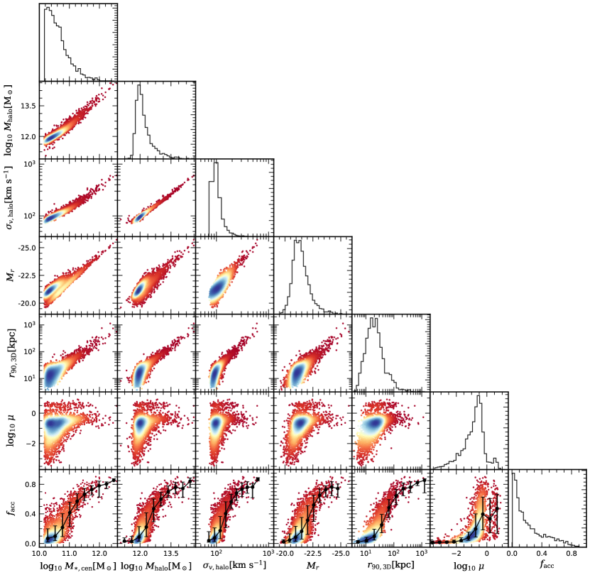
Figure 1: The correlation of a few halo/galaxy features and the ex-situ fraction ($f_{\mathrm{acc}}$), based on central galaxies at $z=0$. The features include $M_{\ast}$, $M_{\mathrm{halo}}$, $\sigma_{v,\mathrm{halo}}$, $M_{r}$, $r_{90,\mathrm{3D}}$ and $\mu$. The readers can find details about these features in Section 2.5, and all the features presented here are calculated in 3-dimensions, rather than in projection. In each panel, the points are colour coded according to the number density distributed over the plane formed by the combination of every two different features, which are smoothed by Gaussian kernels. The diagonal panels show the probability distribution of each feature. The bottom row shows the relationship between $f_{\mathrm{acc}}$ and these features, in which the black lines show the medians of $f_{\mathrm{acc}}$. The errorbars indicate the 16-th to 84-th percentile ranges centred on the medians.

The halo and galaxy features used in this paper (see Section 2) are not independent of each other. Figure 1 demonstrates the correlation among a few most important features in our analysis. The host halo mass of all bound particles ($M_{\mathrm{halo}}$), the velocity dispersion of the host halo ($\sigma_{v,\mathrm{halo}}$), stellar mass ($M_{\ast}$), the $r$-band absolute magnitudes ($M_{r}$) of the galaxy, and the 3-dimensional radius containing 90% of the total bound stellar mass ($r_{90,\mathrm{3D}}$) are all strongly correlated. The correlations of the above features with the maximum merger mass ratio ($\mu$) are weaker but still present.

Fortunately, as we have tested, the learning outcome of the RF method is insensitive to such feature correlations. This is one of the advantages of the RF method. However, the ranking of feature importance is indeed sensitive to such correlations. For example, when both $M_{\ast}$ and $M_{r}$ are included, the importance of $M_{r}$ based on the default output of the RF method (see Section 3.2), is only $\sim$1%. After removing $M_{\ast}$, the learning outcome only changes slightly, but the importance of $M_{r}$ is significantly increased. This is because $M_{\ast}$ already includes most of the information contained in $M_{r}$. $M_{r}$ only carries $\sim$ 1% additional information than $M_{\ast}$, while $M_{\ast}$ perhaps has $>$ 1% additional information than $M_{r}$. Thus $M_{\ast}$ always turns out to have slightly more Information Gain than $M_{r}$ for most of the nodes. In other words, the importance of $M_{r}$ is suppressed by $M_{\ast}$, which makes the output feature importance and their rankings challenging to interpret. This is referred to as the “masking effect" of RF (Louppe, 2014).

To eliminate such confusions, we try an alternative approach to determine the feature importance. We define the importance ranking for each feature based on their $R^{2}$ score ranking (Equation 5), obtained by only including this feature in the RF training and then applying it to the test sample to calculate the score. In this way, the importance of each feature will not be affected by the correlation with other features. In addition, we will also investigate the importances of multiple feature combinations in this paper (see Sections 4.3 and 4.4 for details), and their importance rankings will be represented by the $R^{2}$ score rankings as well, when only including these particular features in the RF model. Notably, upon calculating such $R^{2}$ scores, we have very carefully performed convergence tests to determine the best hyperparameters for each feature or feature combination.

4.2 Overall learning outcome and individual feature importances of 3-dimensional halo and galaxy features

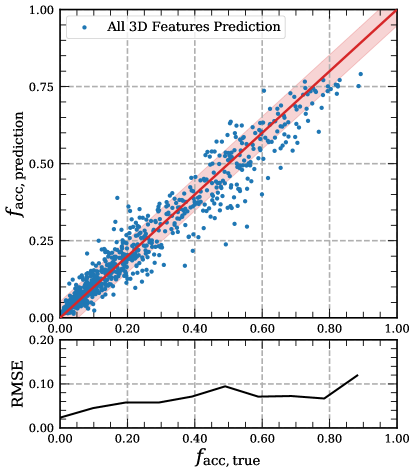
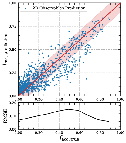
Figure 2: Left: The top panel shows the predicted $f_{\mathrm{acc}}$ based on all available features calculated in 3-dimensions ($y$-axis), versus the true $f_{\mathrm{acc}}$ from the simulation. This is based on central galaxies in TNG100-1, with a mild selection in the magnitude gap with respect to their companions (see Section 2.3.1). The red solid line marks $y=x$, and the red shaded region shows the 1-$\sigma$ standard deviation. The bottom panel shows the root-mean-square error, RMSE (Equation 6), as a function of the true $f_{\mathrm{acc}}$. Right: Similar to the left panel, but the prediction is based on only observable galaxy features calculated in projection.

Table 1: Feature importances of individual halo/galaxy features. The importance value of each feature is represented by the mean $R^{2}$ score of the test samples, when the model is trained using this particular feature (see Section 4.1 for details). The upper limit of the score is 100%. The three columns represent the full, high and low-mass samples used in our analysis. They are all central galaxies in the simulation, with a mild selection in the magnitude gap with respect to their companions (see Section 2.3.1). Features for the full sample are ranked according to the $R^{2}$ scores, while the integer numbers in the brackets for the High-mass and Low-mass columns indicate the ranking, i.e., (1) means the most important feature. The five most important individual features are marked in bold fonts. Note the absolute $R^{2}$ scores of different samples are not directly comparable. One can only compare the absolute scores for the same sample, or compare the change in relative feature importance rankings across different samples.

		Importance (%)
Feature	Full	High-mass	Low-mass
$r_{90,\mathrm{3D}}$	82.12(1)	41.57(1)	70.96(1)
$M_{\mathrm{halo}}$	69.87(2)	36.42(3)	49.64(2)
$M_{\mathrm{200}}$	69.31(3)	34.26(6)	48.82(4)
$R_{\mathrm{200}}$	69.31(4)	34.25(7)	48.82(4)
$M_{\ast}$	67.32(5)	35.52(4)	45.08(6)
$\sigma_{v,\mathrm{halo}}$	66.85(6)	30.70(10)	44.78(7)
$r_{\mathrm{half,halo}}$	64.68(7)	34.42(5)	41.58(8)
$M_{i}$	61.56(8)	32.95(8)	36.38(10)
$\sigma_{v,\ast}$	61.05(9)	25.65(12)	35.36(12)
$r_{50,\mathrm{3D}}$	60.37(10)	38.28(2)	36.20(11)
$J_{\mathrm{halo}}$	59.97(11)	18.03(15)	39.70(9)
$M_{r}$	58.63(12)	32.80(9)	32.72(13)
$V_{\mathrm{max,halo}}$	56.73(13)	28.46(11)	28.08(16)
$\mu$	47.90(14)	18.31(14)	49.11(3)
$\kappa_{\mathrm{rot}}$	43.06(15)	24.12(13)	31.00(14)
$C_{\mathrm{3D}}$	36.44(16)	7.26(17)	30.00(15)
$z_{\mathrm{form}}$	24.15(17)	15.35(16)	22.99(17)
$g-r$	20.46(18)	0.17(19)	12.69(18)
Stellar age	17.02(19)	3.43(18)	4.95(19)

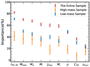
Figure 3: Feature importances of 3-dimensional halo/galaxy features for the full (red), high-mass (orange) and low-mass (blue) galaxy samples, respectively. The errorbars are the 1-$\sigma$ scatters based on randomly dividing the training and test samples 100 times.

The left panel of Figure 2 shows the predicted values of $f_{\mathrm{acc}}$ versus their true values for galaxies in the test sample. The $R^{2}$ score is 93.94%. The $f_{\mathrm{acc}}=f_{\mathrm{acc,true}}$ diagonal line goes well through the data points, indicating no apparent systematic bias. To quantify the scatter, we adopt the root-mean-square error (RMSE):

$$\mathrm{RMSE}=\sqrt{\frac{\sum\limits_{i=1}^{i=n}{\Delta{f_{\mathrm{acc}}^{2}}}}{n}},$$ (6)

where $\Delta{f_{\mathrm{acc}}}=f_{\mathrm{acc,prediction}}-f_{\mathrm{acc,true}}$, and $n$ is the number of galaxies in a given bin of $f_{\mathrm{acc,true}}$. The bottom panel of Figure 2 shows the RMSE as a function of $f_{\mathrm{acc,true}}$. On average, RMSE is 0.068. The right panel of Figure 2 is similar, but is based on the prediction of using only observable galaxy features, which we will discuss later in Section 4.4.

The feature importances for all individual 3-dimensional halo and galaxy features are provided in Table LABEL:tbl:imprank, and for the full, high and low-mass galaxy samples, respectively. For all the three samples, $r_{90,\mathrm{3D}}$ is always the most important. This is somewhat surprising, since $f_{\mathrm{acc}}$ is known to be a strong function of stellar mass (Rodriguez-Gomez et al., 2016). However, as we have checked, the distribution of $f_{\mathrm{acc}}$ indeed tends to show the smallest amount of scatter in Figure 1 when conditioned on $r_{90,\mathrm{3D}}$. This is probably because galaxy size is very closely linked to the accretion history. Dry minor mergers tend to build up the outskirts of galaxies (e.g. Hopkins et al., 2010; Oser et al., 2012; Hilz et al., 2013). Frequent dry minor mergers can cause a considerable growth in size with less amount of increase in the mass of galaxies(e.g. Bédorf & Portegies Zwart, 2013). Observationally, there are also evidences showing that galaxy size is correlated with the environment at fixed stellar mass, though still under debates (e.g. Papovich et al., 2012; Allen et al., 2015; Huang et al., 2018b; Sonnenfeld et al., 2019). Here we also see $r_{90,\mathrm{3D}}$ is more important than $r_{50,\mathrm{3D}}$, because the accreted materials dominate in the outskirts, and thus stars in the outer stellar halo are more strongly correlated with mergers (e.g. Du et al., 2021).

For the full sample, a few global features such as halo mass and size ($M_{\mathrm{halo}}$, $M_{\mathrm{200}}$ and $R_{\mathrm{200}}$) and the stellar mass of galaxies ($M_{\ast}$), are among the top five most important individual features. Here $M_{\mathrm{halo}}$ is defined as the total mass of dark matter particles bound to the main subhalo, which turns out to be slightly more important than the virial mass, $M_{\mathrm{200}}$. This probably reflects that the physically bound particles are more closely related to the formation of the central galaxy than all particles within $R_{200}$. Besides, the halo mass and size features seem to be slightly more important than $M_{\ast}$. However, the typical 1-$\sigma$ uncertainty in the scores is about 2% (full sample), as shown by Figure 3 for a few representative features. Hence the relative ranking for $M_{\mathrm{halo}}$, $M_{\mathrm{200}}$, $R_{\mathrm{200}}$ and $M_{\ast}$ is not very significant compared with the associated uncertainties.

The 6-th and 7-th most important individual features are the total velocity dispersion and the 3-dimensional half-mass radius of the host halo, followed by a few stellar features including the $i$-band absolute magnitude ($M_{i}$), the total velocity dispersion of star particles ($\sigma_{v,\ast}$) and the 3-dimensional half-mass radius of stars ($r_{50,\mathrm{3D}}$). The specific angular momentum of the host halo and the maximum circular velocity, $J_{\mathrm{halo}}$ and $V_{\mathrm{max}}$, are less important than $M_{\mathrm{halo}}$, and the significance is more than 1-$\sigma$ (see Figure 3). $M_{r}$ is less important than $M_{i}$, but with a low significance. Other features quantifying the assembly history, including the maximum merger mass ratio below $z=2$ ($\mu$), halo formation time ($z_{\mathrm{form}}$) and morphology/colour/star formation related features such as $\kappa_{\mathrm{rot}}$, $C_{3D}$, $g-r$ and stellar age, are significantly less important than the other global mass and size features.

For the high-mass sample, $r_{50,\mathrm{3D}}$, $M_{\mathrm{halo}}$, $M_{\ast}$ and $r_{\mathrm{half,halo}}$ are among the top five most important individual features. Compared with the full sample, the rankings of $M_{200}$ and $R_{200}$ now decrease to the 6-th and 7-th. The importances of $\sigma_{v,\mathrm{halo}}$ and $\sigma_{v,\ast}$ also decrease, while the rankings of $M_{r}$, $V_{\mathrm{max,halo}}$ and $\kappa_{\mathrm{rot}}$ slightly increase. In addition, the few least important features with rankings between 16-th and 19-th in the full sample now still have such low importances in the high-mass sample.

For the low-mass sample, the top eight most important individual features are similar to those of the full sample, except that $\mu$ now becomes the third most important individual feature, i.e., its ranking is significantly higher than those in the full and high-mass samples. In addition, the rankings of galaxy concentration, $C_{\mathrm{3D}}$, and halo spin, $J_{\mathrm{halo}}$, increase, but the importances of a few global features such as $M_{r}$, $M_{i}$, $r_{\mathrm{half,halo}}$ and $V_{\mathrm{max,halo}}$ decrease compared with those in the full and high-mass samples.

On average, the fraction of dark matter is more dominant for low-mass satellite galaxies before infall (e.g. Guo et al., 2010). For a similar amount of growth in stellar mass, the growth in the host dark matter halo is stronger for low-mass galaxies, hence a stronger change in the specific angular momentum of the host halo. This probably explains why $J_{\mathrm{halo}}$ has a higher importance ranking than a few other global halo/galaxy features for the low-mass sample.

Interestingly, it seems global halo and stellar features such as the host halo mass, size and stellar mass are significantly more important than assembly history related or morphological features for high-mass galaxies, whereas for low-mass galaxies, the importances of features related to the assembly histories or to the galaxy morphology ($\mu$, $J_{\mathrm{halo}}$ and $C_{\mathrm{3D}}$) have increased.

For both high and low-mass samples, stellar age and $g-r$ colour are not important individually. In fact, we have also checked the importances for the star formation rate and specific star formation rate, which are not directly shown in Table LABEL:tbl:imprank, because they have very low importances individually. This indicates that if only using the current star formation activity or colour of galaxies to predict the accreted stellar mass fraction, the predictive power is very low.

4.3 The feature importance of multiple feature combinations

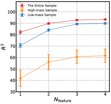
Figure 4: The highest $R^{2}$ score as a function of the number of features used, for the full (red), high-mass (blue) and low-mass (orange) samples, respectively. The $R^{2}$ scores are presented in percentage. The errorbars represent the 1-$\sigma$ scatters of $R^{2}$ scores. The score saturates at three features. Note the absolute $R^{2}$ scores of different samples are not directly comparable.

Table 2: The top five highest $R^{2}$ scores for individual features, two and three feature combinations. This is shown for the full, high-mass and low-mass samples separately. The $R^{2}$ scores are presented in percentage. The 1-$\sigma$ errors in the brackets are given by the scatters among 100 random divisions between the training and test samples. Note the absolute $R^{2}$ scores of different samples are not directly comparable. One can only compare the absolute scores based on the same sample, or compare the change in relative feature importance rankings across different samples.

Sample	$N_{\mathrm{feature}}$	First	Second	Third	Fourth	Fifth
Full	1	$r_{90,\mathrm{3D}}$	$M_{\mathrm{halo}}$	$M_{\mathrm{200}}$	$R_{\mathrm{200}}$	$M_{\ast}$
		82.12($\pm$1.31)	69.87($\pm$1.85)	69.31($\pm$1.93)	69.31($\pm$1.93)	67.32($\pm$2.00)
	2	$r_{90,\mathrm{3D}}$, $\mu$	$r_{50,\mathrm{3D}}$, $\kappa_{\mathrm{rot}}$	$r_{90,\mathrm{3D}}$, $\kappa_{\mathrm{rot}}$	$M_{\mathrm{halo}}$, $\mu$	$r_{90,\mathrm{3D}}$, $z_{\mathrm{form}}$
		89.83($\pm$0.76)	86.39($\pm$0.91)	86.36($\pm$1.03)	85.08($\pm$1.08)	84.85($\pm$1.12)
	3	$r_{90,\mathrm{3D}}$, $\mu$, $\kappa_{\mathrm{rot}}$	$r_{90,\mathrm{3D}}$, $\mu$, $C_{\mathrm{3D}}$	$r_{90,\mathrm{3D}}$, $r_{50,\mathrm{3D}}$, $\mu$	$r_{50,\mathrm{3D}}$, $\mu$, $C_{\mathrm{3D}}$	$r_{50,\mathrm{3D}}$, $\mu$, $\kappa_{\mathrm{rot}}$
		92.80($\pm$0.58)	91.55($\pm$0.66)	91.50($\pm$0.64)	91.36($\pm$0.59)	91.17($\pm$0.65)
High-mass	1	$r_{90,\mathrm{3D}}$	$r_{50,\mathrm{3D}}$	$M_{\ast}$	$M_{\mathrm{halo}}$	$r_{\mathrm{half,halo}}$
		41.75($\pm$7.12)	39.67($\pm$6.22)	35.99($\pm$7.50)	35.94($\pm$7.72)	34.13($\pm$7.61)
	2	$r_{50,\mathrm{3D}}$, $\mu$	$r_{90,\mathrm{3D}}$, $\mu$	$M_{\mathrm{halo}}$, $\mu$	$M_{\ast}$, $\mu$	$M_{\mathrm{200}}$, $\mu$
		55.99($\pm$6.72)	55.23($\pm$6.46)	51.03($\pm$8.44)	50.88($\pm$7.07)	50.38($\pm$8.23)
	3	$r_{50,\mathrm{3D}}$, $\mu$, $\kappa_{\mathrm{rot}}$	$r_{90,\mathrm{3D}}$, $\mu$, $C_{\mathrm{3D}}$	$r_{90,\mathrm{3D}}$, $r_{50,\mathrm{3D}}$, $\mu$	$r_{50,\mathrm{3D}}$, $\mu$, $C_{\mathrm{3D}}$	$r_{90,\mathrm{3D}}$, $\mu$, Stellar Age
		60.70($\pm$5.79)	60.55($\pm$6.14)	59.60($\pm$6.18)	58.51($\pm$6.80)	57.64($\pm$6.46)
Low-mass	1	$r_{90,\mathrm{3D}}$	$M_{\mathrm{halo}}$	$\mu$	$R_{\mathrm{200}}$	$M_{\mathrm{200}}$
		70.60($\pm$1.71)	49.62($\pm$2.70)	48.93($\pm$2.24)	48.75($\pm$2.74)	48.74($\pm$2.72)
	2	$r_{90,\mathrm{3D}}$, $\mu$	$r_{50,\mathrm{3D}}$, $\kappa_{\mathrm{rot}}$	$r_{90,\mathrm{3D}}$, $\kappa_{\mathrm{rot}}$	$M_{\mathrm{halo}}$, $\mu$	$r_{90,\mathrm{3D}}$, $z_{\mathrm{form}}$
		84.05($\pm$1.05)	78.51($\pm$1.18)	78.50($\pm$1.18)	75.87($\pm$1.57)	75.62($\pm$1.60)
	3	$r_{90,\mathrm{3D}}$, $\mu$, $\kappa_{\mathrm{rot}}$	$r_{90,\mathrm{3D}}$, $\mu$, $C_{\mathrm{3D}}$	$r_{90,\mathrm{3D}}$, $r_{50,\mathrm{3D}}$, $\mu$	$r_{50,\mathrm{3D}}$, $\mu$, $C_{\mathrm{3D}}$	$r_{50,\mathrm{3D}}$, $\mu$, $\kappa_{\mathrm{rot}}$
		89.34($\pm$0.78)	86.78($\pm$0.97)	86.74($\pm$0.96)	86.41($\pm$0.93)	86.07($\pm$0.89)

In Section 4.2, we have investigated the importance rankings of different individual features. In Table LABEL:tbl:imprank, we can see that the highest $R^{2}$ score of individual features is 82.12% for the full sample, but a higher $R^{2}$ score of 93.94% can be achieved when all halo and galaxy features are used. This means using only one individual feature to predict $f_{\mathrm{acc}}$ is not enough. However, using a large number of features to determine $f_{\mathrm{acc}}$ could be too redundant in practice. In this sense, we try to determine $f_{\mathrm{acc}}$ with the combination of a limited number of features and investigate the importance rankings of these combinations.

To investigate this, we calculated the $R^{2}$ scores for all possible combinations of every two, three and four features, same as done in Li et al. (2022) and Zhou & Han (2022). The highest $R^{2}$ score with respect to the number of combined features is shown in Figure 4. The red, orange and blue curves are for the full, high and low-mass samples, respectively. The errorbars represent the 1-$\sigma$ scatters by dividing the training and test samples for 100 times. We find the curves become flattened beyond a number of three features, indicating a combination of up to three features can already saturate the score of the prediction. The highest $R^{2}$ score achieved with three features is 92.80% for the full sample, which is very close to the score when all available halo and galaxy features are used (93.94%). This means a lot of information related to $f_{\mathrm{acc}}$ can be well explained by using only three features in combination.

Table LABEL:tbl:imp_combine shows the top five most important features or feature combinations, for the cases of individual features, two and three combined features. We show this for the full, high and low-mass samples separately. Note although we have ranked the different feature combinations in Table LABEL:tbl:imp_combine, the significances in the ranking are not very high compared with the errors ($R^{2}$ scores and associated errors are shown below the feature names).

We find $r_{90,\mathrm{3D}}$, which is the most important single feature, frequently appears in all different combinations as well. For the combination of two features, the five most important cases are often one global mass or size feature ($r_{90,\mathrm{3D}}$, $r_{50,\mathrm{3D}}$, $M_{\mathrm{halo}}$ or $M_{\ast}$), plus another assembly history related or morphological feature ($C_{\mathrm{3D}}$, $\mu$, $\kappa_{\mathrm{rot}}$, $z_{\mathrm{form}}$ or stellar age). For the case of three features, those most important combinations are often one mass/size feature, plus another two assembly/morphological features. In fact, despite the fact that $\mu$ is not very important as an individual feature in the full and high-mass samples, and $\kappa_{\mathrm{rot}}$, for example, is not a very important individual feature in the full, high and low-mass samples, they frequently appear in the most important two and three feature combinations. This indicates that assembly or morphological features carry the most amount of independent information from those in global mass/size features, and thus after combined together, they become the most important. On the other hand, the few top important individual features in Table LABEL:tbl:imprank, such as $r_{90,\mathrm{3D}}$, $M_{\mathrm{halo}}$, $M_{200}$, $R_{200}$ and $M_{\ast}$, are highly correlated with each other, carrying redundant information. This explains why the combination of, for example, $r_{90,\mathrm{3D}}$ and $\mu$, becomes more important than the combination of $r_{90,\mathrm{3D}}$ and $M_{\ast}$ for instance.

Interestingly, we notice two features which are both not very important individually, may become very important after being combined together. For example, the combination of $r_{50,\mathrm{3D}}$ and $\kappa_{\mathrm{rot}}$ rank the second most important for the full sample and the low-mass sample. $r_{50,\mathrm{3D}}$ also appears multiple times in the five most important three feature combinations. However, $r_{50,\mathrm{3D}}$ only ranks the 10-th and 11-th important as an individual feature for the full and low-mass samples. The importance of $\kappa_{\mathrm{rot}}$ as an individual feature is also very low for the full, high and low-mass samples.

Our results show, very promisingly, one can choose to use one global mass or size feature of the galaxy or host halo, in combination with another two features reflecting the assembly history or morphology to predict $f_{\mathrm{acc}}$. In fact, using the combination of $r_{90,\mathrm{3D}}$, $\mu$ and $\kappa_{\mathrm{rot}}$, the RMSE is $\sim$0.072, which is very similar to the RMSE of 0.068 in the left panel of Figure 2, when all available halo and galaxy features are used. In other words, the inclusion of many other halo and galaxy features almost does not help to decrease the RMSE.

In the next subsection, we move on to discuss the RF learning outcome and importance ranking when only observable galaxy features are used.

Table 3: Similar to Table LABEL:tbl:imprank, but shows the individual feature importance rankings for only observable galaxy features in projection. The three most important individual features are marked in bold fonts. Note the absolute $R^{2}$ scores of different samples are not directly comparable. One can only compare the absolute scores for the same sample, or compare the change in relative feature importance rankings across different samples.

		Importance (%)
Feature	Full	High-mass	Low-mass
$M_{\ast}$	64.71(1)	23.43(2)	48.46(1)
$M_{i}$	59.34(2)	14.82(4)	41.79(2)
$M_{r}$	57.33(3)	14.43(6)	39.32(3)
$r_{90,\mathrm{2D}}$	53.18(4)	34.43(1)	36.20(4)
$\sigma_{z,\ast}$	52.59(5)	14.72(5)	31.71(6)
$C_{\mathrm{2D}}$	35.49(6)	7.62(7)	32.31(5)
$r_{50,\mathrm{2D}}$	31.95(7)	20.95(3)	16.50(7)
$g-r$	16.56(8)	7.59(8)	10.10(8)

4.4 The learning outcome and feature importances of observable galaxy features

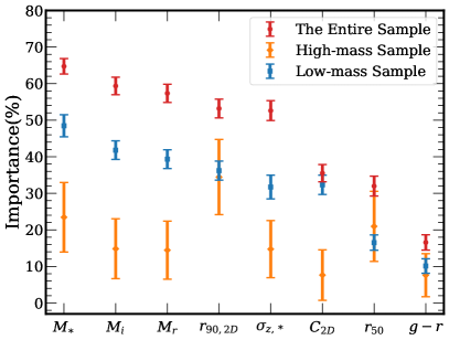
Figure 5: Feature importances of individual observable galaxy features, and for the full (red), high-mass (orange) and low-mass (blue) galaxy samples, respectively. Errorbars are the 1-$\sigma$ scatters based on randomly dividing the training and test samples 100 times. The larger errorbars for the high-mass sample is due to the smaller sample size.

Table 4: The top five most important individual features, two and three feature combinations, and the associated $R^{2}$ scores, for the full, high and low-mass samples. This is only for observable features. The $R^{2}$ scores are presented in percentage. The 1-$\sigma$ scatters in the brackets are given by randomly dividing the training and test samples for 100 times. Note the absolute $R^{2}$ scores of different samples are not directly comparable. One can only compare the absolute scores for the same sample, or compare the change in relative feature importance rankings across different samples.

Sample	$N_{\mathrm{feature}}$	First	Second	Third	Fourth	Fifth
Full	1	$M_{\ast}$	$M_{i}$	$M_{r}$	$r_{90,\mathrm{2D}}$	$\sigma_{z,\mathrm{*}}$
		64.71($\pm$2.11)	59.34($\pm$2.41)	57.33($\pm$2.50)	53.18($\pm$2.57)	52.59($\pm$2.72)
	2	$M_{\ast}$, $r_{90,\mathrm{2D}}$	$M_{\ast}$, $C_{\mathrm{2D}}$	$M_{i}$, $C_{\mathrm{2D}}$	$M_{r}$, $C_{\mathrm{2D}}$	$r_{90,\mathrm{2D}}$, $C_{\mathrm{2D}}$
		70.74($\pm$1.91)	68.97($\pm$1.89)	68.88($\pm$2.01)	68.73($\pm$2.03)	68.16($\pm$1.80)
	3	$M_{\ast}$, $r_{90,\mathrm{2D}}$, $C_{\mathrm{2D}}$	$M_{\ast}$, $C_{\mathrm{2D}}$, $r_{50,\mathrm{2D}}$	$M_{i}$, $r_{90,\mathrm{2D}}$, $C_{\mathrm{2D}}$	$M_{r}$, $r_{90,\mathrm{2D}}$, $C_{\mathrm{2D}}$	$M_{i}$, $C_{\mathrm{2D}}$, $r_{50,\mathrm{2D}}$
		75.76($\pm$1.66)	75.36($\pm$1.66)	74.85($\pm$1.64)	74.70($\pm$1.69)	74.16($\pm$1.71)
High-mass	1	$r_{90,\mathrm{2D}}$	$M_{\ast}$	$r_{50,\mathrm{2D}}$	$M_{i}$	$\sigma_{z,\ast}$
		34.43($\pm$10.28)	23.43($\pm$9.50)	20.95($\pm$9.59)	14.82($\pm$8.19)	14.72($\pm$7.82)
	2	$r_{90,\mathrm{2D}}$, $g-r$	$r_{90,\mathrm{2D}}$, $C_{\mathrm{2D}}$	$r_{90,\mathrm{2D}}$, $r_{50,\mathrm{2D}}$	$r_{90,\mathrm{2D}}$, $\sigma_{z,\ast}$	$r_{90,\mathrm{2D}}$, $M_{\ast}$
		41.37($\pm$9.37)	39.47($\pm$9.88)	39.39($\pm$10.69)	38.04($\pm$10.32)	37.58($\pm$11.10)
	3	$r_{90,\mathrm{2D}}$, $\sigma_{z,\ast}$, $g-r$	$r_{90,\mathrm{2D}}$, $M_{\ast}$, $C_{\mathrm{2D}}$	$r_{90,\mathrm{2D}}$, $M_{\ast}$, $g-r$	$r_{90,\mathrm{2D}}$, $\sigma_{z,\ast}$, $C_{\mathrm{2D}}$	$r_{90,\mathrm{2D}}$, $M_{r}$, $g-r$
		44.23($\pm$9.63)	43.12($\pm$10.72)	42.87($\pm$10.87)	42.80($\pm$10.09)	42.19($\pm$10.40)
Low-mass	1	$M_{\ast}$	$M_{i}$	$M_{r}$	$r_{90,\mathrm{2D}}$	$C_{\mathrm{2D}}$
		48.46($\pm$3.01)	41.79($\pm$2.56)	39.32($\pm$2.56)	36.20($\pm$2.61)	32.31($\pm$2.65)
	2	$M_{\ast}$, $r_{90,\mathrm{2D}}$	$r_{90,\mathrm{2D}}$, $C_{\mathrm{2D}}$	$M_{r}$, $C_{\mathrm{2D}}$	$M_{i}$, $C_{\mathrm{2D}}$	$r_{50,\mathrm{2D}}$, $C_{\mathrm{2D}}$
		56.92($\pm$2.75)	56.25($\pm$2.37)	56.20($\pm$2.56)	55.91($\pm$2.58)	55.75($\pm$2.37)
	3	$M_{\ast}$, $r_{90,\mathrm{2D}}$, $C_{\mathrm{2D}}$	$M_{\ast}$, $r_{50,\mathrm{2D}}$, $C_{\mathrm{2D}}$	$M_{i}$, $r_{90,\mathrm{2D}}$, $C_{\mathrm{2D}}$	$M_{r}$, $r_{90,\mathrm{2D}}$, $C_{\mathrm{2D}}$	$M_{i}$, $C_{\mathrm{2D}}$, $r_{50,\mathrm{2D}}$
		64.48($\pm$2.52)	64.13($\pm$2.51)	63.27($\pm$2.39)	63.15($\pm$2.32)	62.84($\pm$2.44)

The learning outcome and the feature importance rankings based on only observable features are practically more important, which we investigate in this subsection. In the right panel of Figure 2, the predicted values of $f_{\mathrm{acc}}$ are shown against their true values for the test sample when only observable galaxy features calculated in projection are used for training and prediction. The $R^{2}$ score drops to 78.43%, which is lower than the score (93.94%) when all halo and galaxy features calculated in 3-dimensions are used (the left panel of Figure 2). In the bottom panel, the RMSE is on average 0.104, which is $\sim$40% larger than the prediction by using all available halo and galaxy features calculated in 3-dimensions. There are also some biases from the diagonal line at small values of $f_{\mathrm{acc}}$.

Similar to Table LABEL:tbl:imprank, the importance rankings for individual observable features are shown in Table LABEL:tbl:imprankobs, for the full, high and low-mass samples. The scores and associated uncertainties are also presented in Figure 5.

All the features in Table LABEL:tbl:imprankobs have smaller scores compared with corresponding features in Table LABEL:tbl:imprank, especially for $r_{90,\mathrm{2D}}$ and $r_{50,\mathrm{2D}}$. $r_{90,\mathrm{2D}}$ is no longer the most important individual feature for the full and low-mass samples. This is mainly because $r_{90,\mathrm{2D}}$ is calculated based on mock galaxy images involving observational effects such as sky noise, PSF and dust attenuation. Projection plays a relatively minor effect. As we have explicitly checked, if $r_{90}$ is calculated by directly projecting the positions of star particles in the simulation, its importance can be as high as 80.74% (full sample). The inclusion of sky noise has probably made part of the outer stellar halo drop below the noise level, and hence the determination of outer boundaries of galaxies becomes inaccurate (e.g. He et al., 2013; D’Souza et al., 2015), resulting in less correlation with the accreted stellar material. Nevertheless, $r_{90,\mathrm{2D}}$ is still the most important feature for the high-mass sample, while it remains in the top five most important features for the full sample and the low-mass sample. Similar to Table LABEL:tbl:imprank, we find the ranking of $C_{\mathrm{2D}}$ is higher for the low-mass sample.

Based on the same idea as Section 4.2, we also investigate the importance rankings of multiple observable feature combinations. The corresponding results are shown in Table LABEL:tbl:imp_combine_obs for the full, high and low-mass samples. For the full sample, the most important two feature combination is $M_{\ast}$ plus $r_{90,\mathrm{2D}}$. The other important two feature combinations are usually one stellar mass/luminosity or size related feature plus galaxy concentration, $C_{\mathrm{2D}}$, but the difference in the associated $R^{2}$ scores for the top five most important combinations is not significant compared with the errors. For the combination of three observable galaxy features, the scores are further increased. The top five most important combinations are usually one stellar mass/luminosity feature, one galaxy size feature plus $C_{\mathrm{2D}}$. We find $C_{\mathrm{2D}}$, a feature related to observed galaxy morphology in projection, appears very frequently, despite the fact that it is only the 5-th to 7-th most important individual feature in Table LABEL:tbl:imprankobs. This is because it carries the most amount of independent information from galaxy stellar mass and size.

The most important two or three feature combinations for the high and low-mass samples are similar to those for the full sample. However, for the high-mass sample,the line-of-sight velocity dispersion, $\sigma_{z,\ast}$, sometimes appears to replace $M_{\ast}$, and the galaxy $g-r$ colour sometimes appears to replace $C_{\mathrm{2D}}$. Note $g-r$ is the least important feature in Table LABEL:tbl:imprankobs. To summarize, a combination of up to three observable galaxy features of different types, galaxy stellar mass (or line-of-sight velocity dispersion), galaxy size plus a third morphology (or colour) related feature would lead to a score very close to the case when all observable galaxy features are used. In fact, using the combination of $M_{\ast}$, $r_{\mathrm{90,2D}}$ and $C_{\mathrm{2D}}$ for the prediction, the RMSE is $\sim$0.119, which is similar to the RMSE of 0.104 for the right panel of Figure 2.

In the next subsection, we move on to directly compare the bias and scatter in the two cases, and compare with the prediction when only stellar mass is used as the input feature.

4.5 Scatter and bias

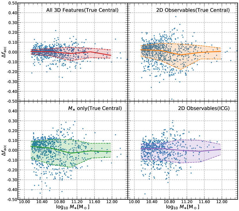
Figure 6: Upper Left: The difference between predicted and true values of $f_{\mathrm{acc}}$ ($\Delta f_{\mathrm{acc}}$), reported as a function of stellar mass. The prediction is based on the learning outcome when all available halo and galaxy features calculated in 3-dimensions are used. Blue dots represent individual haloes/galaxies, while the solid and two dashed lines show the median, 16-th and 84-th percentile boundaries, respectively. Upper Right: The prediction is based on observable galaxy features calculated in projection. Lower Left: $f_{\mathrm{acc}}$ is predicted by only using the stellar mass. Lower Right: Similar to the top right panel, but is based on isolated central galaxies (ICG). Except for the bottom right panel, the test sample used in all the other three panels are based on the same set of central galaxies from TNG100-1. We take one test sample as representative. Other test samples after random divisions can show slightly different results, but the general trends remain very similar. In addition, for all the four panels, the stellar mass in the $x$-axis is the true stellar mass based on all bound star particles from the simulation, although different types of stellar mass are used as input features for the RF training and prediction (see Section 2.5 for details). This is for the sake of fair comparisons.

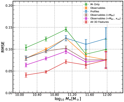
Figure 7: Red, orange and green curves show the root-mean-square errors versus stellar mass, which are based on the RF prediction trained using all available features calculated in 3-dimensions, using only observable features calculated in projection, and using the stellar mass only. These correspond to the upper left, upper right and lower left panels of Figure 6, respectively. The blue curve is based on the RF prediction trained against surface brightness profiles in $gri$-bands, the projected stellar mass density profile, velocity and velocity dispersion profiles, density fluctuation at different radii and the axis ratio of the galaxy. The brown curve is for the prediction when the black hole mass is additionally included as a feature, and on the basis of the brown curve, the magenta curve further includes $\kappa_{\mathrm{rot}}$. Smaller values of RMSE mean better prediction. Errorbars are the 1-$\sigma$ scatters among the results of 100 randomly divided training and test samples. Small shifts along the $x$-axis have been manually added to all curves except the green one, in order to better display the errorbars.

Figure 6 shows the residuals between the predicted and true values of $f_{\mathrm{acc}}$, i.e., $\Delta f_{\mathrm{acc}}$, which is reported as a function of stellar mass. Different panels refer to predictions based on different input features or different samples.

The upper left panel shows the smallest amount of scatter, when all available halo and galaxy features calculated in 3-dimensions are included. Consistent with Figure 2, the scatter gets significantly larger in the upper right panel when only observable galaxy features are used. Despite the significant increase in the amount of scatter, the prediction remains almost unbiased, except for the low-mass end, where we see the data points tend to be skewed towards positive $\Delta f_{\rm acc}$.

Notably, Figure 6 is based on the learning outcome of the full sample. If we plot the results when the high and low-mass samples are trained separately, the scatter becomes slightly smaller at $\log_{10}M_{\ast}/M_{\odot}\sim 11.2$, i.e., the mass threshold used for the division, but remains similar at the high and low-mass ends. Besides, we also note a mild peak in the amount of scatter at $\log_{10}M_{\ast}/M_{\odot}\sim 11$, which is perhaps related to the transition in the relation between $f_{\mathrm{acc}}$ and stellar mass at $\log_{10}M_{\ast}/M_{\odot}\sim 11$, as the readers can see from the bottom left panel of Figure 1 that the scatter in $f_{\mathrm{acc}}$ seems to be slightly larger at $\log_{10}M_{\ast}/M_{\odot}\sim 11$. Galaxies with $\log_{10}M_{\ast}/M_{\odot}\sim 11$ represent a transition stage from blue star-forming disks to red passive ellipticals. Perhaps the modelling of these galaxies more strongly depends on a few other features, which are so far not included in our analysis, such as the redshift when the star formation activity of the galaxy starts to quench.

The difference between the two upper panels of Figure 6 reflects the fact that observable galaxy features are not enough to capture the full information of $f_{\mathrm{acc}}$. The prediction in the upper left panel is also based on a few unobservable features such as host halo mass, size, specific angular momentum and assembly histories. These have helped to reduce the scatter and bias significantly. In addition, other features used in the upper left panel, if observable, are in fact calculated in 3-dimensions without including observational noise and projection effects, which also improves the prediction.

Since the stellar mass is among one of the most important observable features, it is interesting to show the ability of predicting $f_{\mathrm{acc}}$ using stellar mass solely. This is shown in the lower left panel of Figure 6. Compared with the upper right panel, the amount of bias and scatter is slightly larger. At $\log_{10}M_{\ast}/M_{\odot}<11.1$, the distribution is a bit more asymmetric. Therefore the inclusion of a few other observable galaxy features indeed helps to bring some mild improvements than simply using stellar mass.

We also investigate whether the sample selection in real observation might affect the learning outcome. As mentioned in Section 2.3.2, we cannot directly identify true halo central galaxies in real observations, which are often selected through indirect or empirical approaches. Here we repeat our RF training against a sample of isolated central galaxies (see details in Section 2.3.2), using only observable galaxy features calculated in projection. The scatter in predicted versus true values of $f_{\mathrm{acc}}$ based on the corresponding test sample is presented in the lower right panel of Figure 6. This is to be directly compared with the upper right panel. As have been mentioned, the selection of isolated central galaxies would introduce a small amount of contamination by satellite galaxies, but our results do not seem to be significantly affected by such satellite contamination, i.e., the scatter in the lower right panel seems to be even slightly smaller than that of the upper right panel. The slight decrease in the scatter of the lower right panel is perhaps due to the sample selection and statistical fluctuation.

Figure 7 directly compares the three cases, by overplotting the RMSEs of the upper left, upper right and lower left panels of Figure 6 together. It is clearly shown that when only observable galaxy features are used, the RMSE of $f_{\mathrm{acc}}$ can be decreased by $\sim$0.03 (20%) than purely using stellar mass for the prediction. When all available halo and galaxy features calculated in 3-dimensions are included, the scatter can be further reduced by $\sim$0.04. The amount of improvements is almost a constant at $\log_{10}M_{\ast}/M_{\odot}<11$, which is slightly smaller at $\log_{10}M_{\ast}/M_{\odot}\geqslant 11$, perhaps indicating for high-mass galaxies, more information about $f_{\mathrm{acc}}$ is included in other features in addition to stellar mass and other unobservable features so far not included in our analysis. Consistent with Figure 6, the RMSE itself also shows weak dependence on stellar mass, with a peak at $\log_{10}M_{\ast}/M_{\odot}\sim 11$, which slightly decreases towards both low and high-mass ends. Note when we only use the three most important features in combination to predict $f_{\mathrm{acc}}$ (all available features or observable features, see Tables LABEL:tbl:imp_combine and LABEL:tbl:imp_combine_obs) , the scatters are very similar to the red or orange curves in Figure 7.

So far, after including all observable galaxy features in the RF training for prediction, the RMSE is about 0.1 in $f_{\mathrm{acc}}$, which gently decreases to $\sim 0.08$ at the low and high-mass ends. One interesting question to ask is what is the best we can achieve, if we input entire galaxy images or velocity maps for training and prediction? We move on to investigate this in the next section.

5 Discussion

5.1 Using density and velocity profiles for prediction

Table 5: Feature importances ($R^{2}$ scores) for the projected stellar mass densities, line-of-sight velocity and velocity dispersions measured at different radii. We do not provide results for surface brightness profiles in $gri$-bands, which actually show similar trends as the projected stellar mass density profile. The profiles are calculated for 10 radial bins between 0.31 and 3.16 times the projected radius containing half of the stellar mass ($r_{50}$).

		Importance (%)
$r/r_{50}$	0.36	0.45	0.57	0.71	0.90	1.13	1.42	1.79	2.25	2.84
velocity dispersion profile	44.57	41.81	38.95	35.67	31.44	27.24	22.24	19.30	17.77	16.84
density profile	16.88	19.94	21.66	21.91	21.50	20.89	19.51	16.71	12.52	8.07
velocity profile	5.82	5.33	5.12	4.77	4.22	3.36	2.84	2.28	2.13	2.07

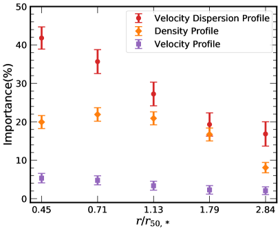
Figure 8: The feature importances for the projected stellar mass densities, line-of-sight velocities and velocity dispersions measured at different radii (red dots, orange diamonds and purple squares, see the legend). Errorbars are the 1-$\sigma$ scatters among the results of 100 randomly divided training and test samples.

In this subsection, we try to test what is the best one can achieve to predict $f_{\mathrm{acc}}$ with current and future observations. In principle, we can input the entire galaxy image in all available filters for training. We can also include the velocity map based on current or future integral field unit (IFU) observations. The images and velocity maps themselves should contain the maximum amount of information so far we can observe for a given galaxy. Since the training based on entire galaxy images is not efficient with the RF method, we choose to represent the image using the surface brightness profiles in $gri$-bands and the projected stellar mass density profile. The velocity map is represented by the mean line-of-sight velocity and velocity dispersion profiles, and we choose the $z$-axis of the simulation to represent the line-of-sight direction. We use these profiles as input features. We also postpone analysis based on galaxy images and velocity maps to future studies with alternative machine learning algorithms such as the neural network.

To calculate the various kinds of profiles, we adopt 10 radial annuli between 0.31 and 3.16 times the projected radius containing half of the stellar mass. We have explicitly checked that our RF learning outcome and feature importance ranking are not sensitive to how the binning is chosen, as long as the number of bins is in a reasonable range. Moreover, TNG galaxies are not strictly spherical, and for a given radial annulus, the actual density and surface brightness distribution can vary within the annulus. Thus we also include the axis ratio of the entire galaxy and the density fluctuations at different radii as input features. However, the scores for these features are low, which help little to improve the prediction, and thus we do not directly show their importances. We have also tried to include the covariance matrixes for all these profiles as input features, and we end up with almost no improvements.

Blue lines and symbols in Figure 7 show the RMSEs of the learning outcome based on all the different kinds of profiles mentioned above, as a function of stellar mass. Compared with the orange lines and symbols, which have been discussed in Section 4.5, the blue lines and symbols have slightly smaller values at $\log_{10}M_{\ast}/M_{\odot}\sim 10.6$, whereas the RMSEs in the two most massive bins even become larger though the errors are also quite large. Therefore, it seems even after we use up all the information contained in the projected density, surface brightness, line-of-sight velocity and velocity dispersion profiles, very limited improvements can be achieved. This is probably because for mergers/accretions happened early on, stars have enough time to be phase mixed, leaving less amount of information about the merger histories in the density and velocity maps. Maybe further including tangential velocities and metallicity gradients can help to achieve more improvements, though tangential velocities can be extremely difficult or impossible to measure for distant extra-galactic systems. In addition, satellite galaxies can continue forming stars after falling into the current host halo. The amount of stellar mass formed after infall also contributes to the ex-situ stellar mass. Further including features related to the star formation activities and orbits of satellites after infall might help to improve.

The feature importances for the projected stellar mass density profile, the line-of-sight velocity and velocity dispersion profiles measured at different projected radii are presented in Table LABEL:tbl:imprankprofile and Figure 8. We only plot 5 out of the 10 radial bins in Figure 8 to make the figure easy to read. In Figure 8, the red dots are all above the purple squares, especially for those points in more central regions, indicating that the second moments in velocity carry significantly more information than the first moments. Besides, it seems the projected stellar mass density profiles are significantly less important than the second moments in velocity as well, but are more important than the first moments in velocity, with the orange diamonds in the middle of red dots and purple squares.

Indeed, substructures formed by mergers are expected to preserve better their clustering in the full 6-dimensional phase space. As a result, many previous studies look for tidal debris and substructures around our Milky Way Galaxy and also extra-galactic galaxies with IFU observations in velocity, energy and action spaces (e.g. Helmi, 2004; Myeong et al., 2018b, a; Belokurov et al., 2018; Yuan et al., 2020; Du et al., 2021; Zhu et al., 2021). The fact that we found the second moments in the velocity are more important than the density distribution is consistent with the expectation, proving that numerical simulations performed under the standard hierarchical structure formation theory of our Universe is capable of producing such a trend. Moreover, Figure 8 also shows that the importance of the velocity dispersion profiles shows a dependence on the radius, i.e., the velocity dispersion in the central region is more important. This is perhaps because tidal debris is more phase mixed in central regions of their hosts (e.g. Wang et al., 2015), and thus velocity dispersion information becomes more important to disentangle the in-situ and ex-situ components.

The fact that even after including the entire projected density, surface brightness, line-of-sight velocity and velocity dispersion profiles, the scatter in the learning outcome is not significantly improved, indicates that multi-component decomposition of the surface brightness profiles would suffer from similar or even worse amount of uncertainties, compared with the orange or blue solid lines in Figure 7.

5.2 Improvements with future observations

So far we did not include the mass of central black holes, $M_{\mathrm{BH}}$, in our list of features. Observations have revealed tight correlations between the mass of central supermassive black holes and properties of host galaxies, such as the velocity dispersion, mass and luminosity of the bulge component, total stellar mass and velocity dispersion of the host (see e.g. Kormendy & Ho, 2013, for a review). These relations indicate strong co-evolution of central black holes and their host galaxies. In many previous studies, this is often interpreted as the outcome of galaxy mergers, which contribute to the growth in mass of both central black holes and host galaxies (e.g. Croton et al., 2006; Hopkins et al., 2006; Peng, 2007; Kormendy & Bender, 2011; Mannerkoski et al., 2021), though many other studies also proposed merger-free scenarios to interpret the co-evolution (e.g. Kormendy & Kennicutt, 2004; Greene et al., 2010; Oh et al., 2012; Simmons et al., 2013).

According to the above background scenario, $f_{\mathrm{acc}}$ might be correlated with $M_{\mathrm{BH}}$. Observationally, $M_{\mathrm{BH}}$ is difficult but still possible to measure, through, for example, reverberation mapping of AGN broad line regions (e.g. Blandford & McKee, 1982). We thus examine the learning outcome when $M_{\mathrm{BH}}$ is used as an observable. The brown lines and symbols in Figure 7 show the RMSE after further including $M_{\mathrm{BH}}$ as an observable feature. Compared with the blue lines and symbols, the RMSE is further reduced by at least $\sim$20% at $\log_{10}M_{\ast}/M_{\odot}>11$, but the error of the most massive data point is very large. There are very weak improvements at the low-mass end. If $M_{\mathrm{BH}}$ can be accurately measured in future observations, the prediction of $f_{\mathrm{acc}}$ by additionally including $M_{\mathrm{BH}}$ is promising to be further improved by at least $\sim$20% for massive galaxies, though this conclusion might depend on the subgrid physics, as TNG is not capable of resolving black hole mergers.

In fact, as we have checked, in TNG100, $M_{\mathrm{BH}}$ is very strongly correlated with the host halo mass defined through all bound particles, $M_{\mathrm{halo}}$, with a considerably smaller amount of scatter than that between $M_{\ast}$ and $M_{\mathrm{halo}}$. Thus the inclusion of $M_{\mathrm{BH}}$ is a very good reflection of the host halo mass for central galaxies in TNG, resulting in such a significant improvement in the prediction of $f_{\mathrm{acc}}$ for massive galaxies. However, also due to this strong correlation, if further including $M_{\mathrm{BH}}$ in the list of all halo and galaxy features calculated in 3-dimensions, the improvement is weak, i.e., the RMSE is similar to the red lines and symbols in Figure 7.

Many existing studies have used the abundance, total luminosity or total stellar mass of satellite galaxies as a proxy to the host halo mass (e.g. Wang & White, 2012; Sales et al., 2013; Graham et al., 2019; Wang et al., 2021c). We did not include these satellite related features in our analysis due to the concern of the TNG100 resolution limit. Besides, in current spectroscopic observations, it is difficult to measure the satellite abundance down to faint magnitudes. Many small satellites do not have spectroscopic observations. The method of counting and averaging photometric satellites around spectroscopically identified central galaxies, with statistical background subtraction or modelling of photometric redshift errors (e.g. Wang et al., 2011; Guo et al., 2012; Lan et al., 2016; Wang et al., 2019b; Wang et al., 2021a; Xu & Jing, 2021), cannot achieve satellite counts for individual systems. However, on-going and future deep spectroscopic surveys such as the Dark Energy Spectroscopic Instrument (DESI; DESI Collaboration et al., 2016), will provide spectroscopic measurements for much fainter satellites. We thus further check the amount of improvements after including the total stellar mass in satellites more massive than $10^{8}M_{\odot}$ as an observable feature. Unfortunately, the improvement is very limited, which is at most $\sim$1% at $\log_{10}M_{\ast}/M_{\odot}\sim 11.1$. In particular, the corresponding score is 52.19% for the full sample, and the small improvement is mainly due to its correlation with $M_{\ast}$ in TNG.

In addition to $M_{\mathrm{BH}}$ and satellites, another feature, $\kappa_{\mathrm{rot}}$, which is not considered as an observable in our analysis above, is in fact closely related to the so-called spin parameter of galaxies. The spin parameter quantifies the specific angular momentum, which can be estimated for galaxies with good IFU data (e.g. Cappellari, 2016; Graham et al., 2019; Wang et al., 2020; Zhu et al., 2021). The magenta lines and symbols in Figure 7 show the RMSE after further including $\kappa_{\mathrm{rot}}$ as an observable, together with $M_{\mathrm{BH}}$. The inclusion of $\kappa_{\mathrm{rot}}$ further decreases the RMSE for smaller galaxies. Since $M_{\mathrm{BH}}$ is more important for massive galaxies, the joint inclusion of $M_{\mathrm{BH}}$ and $\kappa_{\mathrm{rot}}$ help to decrease the RMSE by $\sim$20% over the entire mass range. Note our analysis is based on the true values of $M_{\mathrm{BH}}$ and $\kappa_{\mathrm{rot}}$ from the simulation, without any observation and projection effects. So the 20% of improvement should be understood as an estimate of the upper limit for what we can achieve, if $M_{\mathrm{BH}}$ and $\kappa_{\mathrm{rot}}$ can be accurately determined with future observations.

The fact that $r_{90,\mathrm{3D}}$ is the most important feature is very promising. Our results show that after including the sky noise and PSF of SDSS, the importance of $r_{90,\mathrm{2D}}$ drops. However, on-going and future deep imaging surveys and instruments, such as the Hyper Suprime-Cam (HSC) Imaging Survey (Miyazaki et al., 2012, 2018; Komiyama et al., 2018; Furusawa et al., 2018), the Large Synoptic Survey Telescope (LSST; Ivezić et al., 2008) and the China Space Station Telescope (CSST; Zhan, 2011; Cao et al., 2018; Gong et al., 2019) are promising to achieve significantly better resolution and deeper imaging of the outer stellar halo, hence improving the measurement of $r_{90,\mathrm{2D}}$ and the prediction of $f_{\mathrm{acc}}$.

5.3 Can the learning outcome be directly applied to real galaxies?

In this subsection, we further discuss the feasibility and uncertainty of applying our RF learning outcome based on TNG100-1 galaxies to real galaxies. We have shown that the inclusion of other observable galaxy features in addition to stellar mass can lead to $\sim$0.03 (20%) of decrease in the RMSE, so the RF prediction based on all these features jointly is indeed more precise than simply predicting $f_{\mathrm{acc}}$ based on only stellar mass. Moreover, even after including almost all available information from galaxy images and velocity maps, the uncertainty in the prediction of $f_{\mathrm{acc}}$ is about 0.1, which gently decreases to $\sim 0.08$ at the low and high-mass ends. This is perhaps the limit one can achieve with current observations.

However, to apply the RF learning outcome based on TNG galaxies to real observed galaxies, we care about how TNG agrees with the real data. Disagreement between TNG predictions and the real Universe would introduce systematic uncertainties. It has been shown in previous studies that TNG predictions still deviate from real data, in terms of a few detailed and stringent comparisons, such as the mass-size relation, morphological and colour features.

For example, by comparing the mass-size relation of SDSS and GAMA galaxies with TNG predictions, Pillepich et al. (2018) showed that TNG galaxies tend to have larger sizes than those of real galaxies at fixed stellar mass. Moreover, Genel et al. (2018) quantitatively estimated that the discrepancies between the sizes of TNG100 and real galaxies are in the range of $\sim$0 to 0.2dex, which is sensitive to sample selections and size definitions in both observations and simulations.

In addition to the mass-size relation, tensions also exist when comparing the morphology of TNG and observed galaxies. For example, Rodriguez-Gomez et al. (2019) compared synthetic galaxy images from TNG and Pan-STARRS observations. It was reported that TNG galaxies show good overall agreement with real data. The median trends of morphological, size and shape features with respect to stellar mass are consistent with the observational trends within 1-$\sigma$. However, TNG has difficulties in reproducing a strong morphology-colour relation, which is probably due to inefficient feedback near the galaxy centre, and thus TNG galaxies are too concentrated. With deep learning classifications, the mass-size relations of TNG galaxies divided by morphological types agree well with the relations of real galaxies, but the correlation between optical morphology and Sérsic index is weaker than SDSS (Huertas-Company et al., 2019). Moreover, Zanisi et al. (2021) announced that TNG simulations still cannot reproduce the details of galaxy morphology structures on small scales very well, especially for those quenched spheroidal galaxies, which could be related to the coarse numerical resolution.

Delicated disagreement also exists in the outer stellar haloes and host dark matter haloes between TNG and real observed galaxies. Merritt et al. (2020) compared a few galaxies from the Dragonfly Nearby Galaxies Survey with TNG mass-matched counterparts, and found that real galaxies have less mass or light at large radii, which they denote as a so-called “missing outskirts problem". The inconsistency might be related to their small sample of nearby galaxies, which is not large enough to achieve good statistical significance, but it might also indicate the necessity of a finer tuning in satellite disruption in TNG. More recently and combining weak lensing measurements, Ardila et al. (2021) reported that at the virial mass of $\sim 10^{13}M_{\odot}$, the outer stellar mass profile of massive galaxies at $z\sim 0.4$ is in excellent agreement with TNG predictions, whereas at $\sim 10^{14}M_{\odot}$, TNG shows excess in the outer stellar mass, though the effect of extended PSF wings (e.g. Wang et al., 2019a) is not carefully corrected. Moreover, Renneby et al. (2020) claimed that TNG300 tends to predict $\sim$50% more lensing signals for red galaxies with $10.2<\log_{10}M_{\ast}/M_{\odot}<11.1$ at a projected distance of 0.6Mpc/h to the galaxy centre.

At the massive end, the stellar mass and luminosity functions of simulated and observed galaxies often show discrepancies, which might be due to the missing outskirts of observed galaxies below the sky noise level of shallow surveys (e.g. He et al., 2013; D’Souza et al., 2015; Huang et al., 2018a). Such a discrepancy can be significantly reduced after adopting some aperture cuts to simulated galaxies (Pillepich et al., 2018), but does not totally disappear.

According to the studies mentioned above, further improvements are still required to bring better agreement between TNG predictions and real observations, especially in terms of galaxy size and morphology. In our analysis of this paper, we found up to three features related to stellar mass, galaxy size and morphology capture the most amount of information upon determining $f_{\mathrm{acc}}$. Since TNG galaxy size and morphology still show mismatches with observations, applying our current RF model directly to real data can be problematic. Note, however, the tension with real observation is not a unique problem to only TNG, but stays as a challenge to many other hydrodynamical simulations as well. For instance, the galaxy sizes predicted by the EAGLE (Evolution and Assembly of GaLaxies and their Environments simulations; Schaye et al., 2015; Crain et al., 2015) suite of simulations were also reported to be larger than real observed galaxies (e.g. Van de Sande et al., 2019; Yang et al., 2021a; De Graaff et al., 2022). Moreover, Bignone et al. (2020) reported that the distribution of non-parametric morphological statistics based on mock and real observed galaxy images still present non-negligible differences, which is true for both TNG and EAGLE.

As a result, efforts are still necessary to bring in better agreements between predictions by modern hydrodynamical simulatsions and real data, before we can finally apply our RF model to real observations. However, our results do suggest that a joint modelling of all or up to three different observable features based on the RF machine learning approach can lead to a precision of about 0.1 in the prediction of $f_{\mathrm{acc}}$, and if the central black hole mass and spin parameter of galaxies can be accurately measured in future observations, the uncertainty can be further decreased by $\sim$20%. Hence the RF learning outcome is promising to be applied to future simulations and observations. Notably, we have repeated our analysis with the higher resolution TNG50 simulations. Though the numbers of galaxies in the training and test samples significantly decrease due to the smaller box size, our conclusions about the feature importance rankings remain very similar.

6 Conclusions

Using the TNG100-1 simulation and the random forest (RF) machine learning approach, we have performed a comprehensive study on the importance ranking of various halo/galaxy features and the prediction of the ex-situ stellar mass fractions ($f_{\mathrm{acc}}$) for galaxies with $\log_{10}M_{\ast}/M_{\odot}>10.16$. The amount of bias and scatter in the learning outcome is carefully investigated.

The default feature importance ranking returned by the RF method suffers from the so-called masking effect when there are strong correlations among input features. We thus use the $R^{2}$ score based on each individual feature and different feature combinations to quantify the importance ranking.

We find for high-mass galaxies within $\log_{10}M_{\ast}/M_{\odot}>11.20$, global halo and galaxy features, including the virial mass of the host halo, the total mass of all bound particles, the virial radius of the host halo and the stellar mass of the galaxy, are among the few most important features. For low-mass galaxies with $10.16<\log_{10}M_{\ast}/M_{\odot}\leqslant 11.20$, the importances for features reflecting halo assembly histories and galaxy morphologies are increased. This is very probably because the star formation of low-mass galaxies is dominated less by the shallower potential of the host halo, and could be more stochastic and sensitive to merger histories.

For the full, low and high-mass samples of galaxies used in our analysis, we found the radius containing 90% of the total stellar mass, calculated in 3-dimensional spherical shells, $r_{90,\mathrm{3D}}$, always has the highest importance. This is probably because $r_{90,\mathrm{3D}}$ defined in this way is close to the boundaries of galaxies and probes well the mass accreted and deposited in the outskirts of galaxies. However, if it is calculated from mock galaxy images in projection, after involving dust attenuation, the PSF and sky noise from SDSS, the importance of $r_{90,\mathrm{2D}}$ decreases, though it is still among the few most important observable features. This is mainly caused by the inclusion of sky noise and other observational effects, while projection plays a minor role. Compared with $r_{90,\mathrm{3D}}$, the importance of $r_{50,\mathrm{3D}}$ as an individual feature is significantly lower, indicating it is the outer stellar halo more strongly correlated with mergers. For the full, high and low-mass samples, the $g-r$ colour, stellar age and star formation rate are all not important individually.

We find a combination of up to three features with different types can already saturate the predictive power. Theoretically, the combination of one global feature related to halo/galaxy mass or size, another feature reflecting the halo assembly history and a third morphological feature such as galaxy concentration, can lead to scores very close to the case when all available halo and galaxy features calculated in 3-dimensions are used. Observationally, the combination of galaxy stellar mass, galaxy size and a third feature reflecting galaxy morphology can lead to scores very similar to the case when all observable features are used. For more massive galaxies, stellar mass can be replaced by the line-of-sight velocity dispersion, and the morphological feature can be replaced by galaxy $g-r$ colour.

When all available halo and galaxy features calculated in 3-dimensions are used, the RF learning outcome gives a small amount of scatter, with an average RMSE of 0.068 in $f_{\mathrm{acc}}$. If using the combination of three features quantifying galaxy size, assembly history and morphology, the RMSE is already as small as 0.072. On the other hand, when only observable galaxy features calculated in projection are used, the bias is still negligible, except for the low-mass end. However, the scatter is significantly increased, with the average RMSE of $f_{\mathrm{acc}}$ increasing to 0.104, which shows only weak dependence on stellar mass. Nevertheless, if compared with the case when only stellar mass is used for training and prediction, the inclusion of other observable galaxy features can indeed help to decrease the amount of scatter by $\sim$20%. If using the combination of three observable features quantifying galaxy stellar mass, size and morphology, the RMSE is already as small as 0.119.

To understand what is the best we can achieve with current observations, we tried to use the entire projected stellar mass density profile, surface brightness profiles in $gri$-bands, the velocity and velocity dispersion profiles, the density fluctuation at different radii and the axis ratio of the galaxy as input features. We found velocity dispersions are more important than the surface density profiles, while the mean velocities are the least important. It turns out that the scatter in the learning outcome is only slightly improved by $\sim$5% at $\log_{10}M_{\ast}/M_{\odot}<11.1$ after including all these profiles. The profiles included in this way are expected to represent the entire galaxy image and velocity map, and thus carry approximately the maximum amount of information that we can observe. The limited amount of improvements perhaps implies that the merger histories cannot be fully captured by the density and velocity maps, especially for stars merged a long time ago and are more completely phase mixed with the in-situ component.

With current observations, it is thus difficult to constrain $f_{\mathrm{acc}}$ better than a precision of $\sim$0.1. Our findings also indicate that multi-component decomposition based on the surface brightness profiles galaxies should suffer from at least a similar or even worse amount of uncertainties than our RF approach.

We find the inclusion of the central black hole mass as an observable can further decrease the scatter for massive galaxies. If additionally including the spin parameter of the host galaxies as an observable, the scatter can be improved for smaller galaxies. The central black hole mass is very strongly correlated with the host halo mass in TNG100. In the future, if the central black hole mass and the spin parameter of galaxies can be more accurately determined in observation, the scatter is promising to be further reduced by $\sim$20%.

Data availability

Data available to share upon request.

References

- Abazajian et al. (2009) Abazajian K. N., et al., 2009, The Seventh Data Release of the Sloan Digital Sky Survey (arXiv:0812.0649), doi:10.1088/0067-0049/182/2/543
- Allen et al. (2015) Allen R. J., et al., 2015, ApJ, 806, 3
- Ardila et al. (2021) Ardila F., et al., 2021, MNRAS, 500, 432
- Avila et al. (2014) Avila S., et al., 2014, MNRAS, 441, 3488
- Baes et al. (2011) Baes M., Verstappen J., De Looze I., Fritz J., Saftly W., Vidal Pérez E., Stalevski M., Valcke S., 2011, ApJS, 196, 22
- Bédorf & Portegies Zwart (2013) Bédorf J., Portegies Zwart S., 2013, MNRAS, 431, 767
- Belokurov et al. (2018) Belokurov V., Erkal D., Evans N. W., Koposov S. E., Deason A. J., 2018, MNRAS, 478, 611
- Bignone et al. (2020) Bignone L. A., Pedrosa S. E., Trayford J. W., Tissera P. B., Pellizza L. J., 2020, MNRAS, 491, 3624
- Blandford & McKee (1982) Blandford R. D., McKee C. F., 1982, ApJ, 255, 419
- Blanton et al. (2001) Blanton M. R., et al., 2001, AJ, 121, 2358
- Breiman (2001) Breiman L., 2001, Machine Learning, 45, 5
- Breiman et al. (1983) Breiman L., Friedman J. H., Olshen R. A., Stone C. J., 1983.
- Bullock & Johnston (2005) Bullock J. S., Johnston K. V., 2005, ApJ, 635, 931
- Camps & Baes (2015) Camps P., Baes M., 2015, Astronomy and Computing, 9, 20
- Cao et al. (2018) Cao Y., et al., 2018, MNRAS, 480, 2178
- Cappellari (2016) Cappellari M., 2016, ARA&A, 54, 597
- Carrasco Kind & Brunner (2013) Carrasco Kind M., Brunner R. J., 2013, MNRAS, 432, 1483
- Cheng et al. (2011) Cheng J. Y., Faber S. M., Simard L., Graves G. J., Lopez E. D., Yan R., Cooper M. C., 2011, MNRAS, 412, 727
- Cooper et al. (2010) Cooper A. P., et al., 2010, MNRAS, 406, 744
- Crain et al. (2015) Crain R. A., et al., 2015, MNRAS, 450, 1937
- Croton et al. (2006) Croton D. J., et al., 2006, MNRAS, 365, 11
- DESI Collaboration et al. (2016) DESI Collaboration et al., 2016, arXiv e-prints, p. arXiv:1611.00036
- D’Souza et al. (2014) D’Souza R., Kauffman G., Wang J., Vegetti S., 2014, MNRAS, 443, 1433
- D’Souza et al. (2015) D’Souza R., Vegetti S., Kauffmann G., 2015, MNRAS, 454, 4027
- Davis et al. (1985) Davis M., Efstathiou G., Frenk C. S., White S. D. M., 1985, ApJ, 292, 371
- De Graaff et al. (2022) De Graaff A., Trayford J., Franx M., Schaller M., Schaye J., van der Wel A., 2022, MNRAS, 511, 2544
- Du et al. (2021) Du M., Ho L. C., Debattista V. P., Pillepich A., Nelson D., Hernquist L., Weinberger R., 2021, ApJ, 919, 135
- Furusawa et al. (2018) Furusawa H., et al., 2018, PASJ, 70, S3
- Genel et al. (2018) Genel S., et al., 2018, MNRAS, 474, 3976
- Gong et al. (2019) Gong Y., et al., 2019, ApJ, 883, 203
- Graham et al. (2005) Graham A. W., Driver S. P., Petrosian V., Conselice C. J., Bershady M. A., Crawford S. M., Goto T., 2005, AJ, 130, 1535
- Graham et al. (2019) Graham M. T., Cappellari M., Bershady M. A., Drory N., 2019, arXiv e-prints, p. arXiv:1910.05139
- Greene et al. (2010) Greene J. E., et al., 2010, ApJ, 721, 26
- Guo et al. (2010) Guo Q., White S., Li C., Boylan-Kolchin M., 2010, MNRAS, 404, 1111
- Guo et al. (2012) Guo Q., Cole S., Eke V., Frenk C., 2012, MNRAS, 427, 428
- Han et al. (2019) Han J., Li Y., Jing Y., Nishimichi T., Wang W., Jiang C., 2019, MNRAS, 482, 1900
- He et al. (2013) He Y. Q., Xia X. Y., Hao C. N., Jing Y. P., Mao S., Li C., 2013, ApJ, 773, 37
- Helmi (2004) Helmi A., 2004, ApJ, 610, L97
- Henriques et al. (2015) Henriques B. M. B., White S. D. M., Thomas P. A., Angulo R., Guo Q., Lemson G., Springel V., Overzier R., 2015, MNRAS, 451, 2663
- Hilz et al. (2013) Hilz M., Naab T., Ostriker J. P., 2013, MNRAS, 429, 2924
- Hopkins et al. (2006) Hopkins P. F., Somerville R. S., Hernquist L., Cox T. J., Robertson B., Li Y., 2006, ApJ, 652, 864
- Hopkins et al. (2010) Hopkins P. F., et al., 2010, ApJ, 715, 202
- Huang et al. (2018a) Huang S., Leauthaud A., Greene J. E., Bundy K., Lin Y.-T., Tanaka M., Miyazaki S., Komiyama Y., 2018a, MNRAS, 475, 3348
- Huang et al. (2018b) Huang S., et al., 2018b, MNRAS, 480, 521
- Huertas-Company et al. (2019) Huertas-Company M., et al., 2019, MNRAS, 489, 1859
- Hunter (2007) Hunter J. D., 2007, Comput. Sci. Eng., 9, 90
- Ivezić et al. (2008) Ivezić Ž., et al., 2008, preprint, (arXiv:0805.2366)
- Karademir et al. (2019) Karademir G. S., Remus R.-S., Burkert A., Dolag K., Hoffmann T. L., Moster B. P., Steinwandel U. P., Zhang J., 2019, MNRAS, 487, 318
- Komiyama et al. (2018) Komiyama Y., et al., 2018, PASJ, 70, S2
- Kormendy (1977) Kormendy J., 1977, ApJ, 217, 406
- Kormendy & Bender (2011) Kormendy J., Bender R., 2011, Nature, 469, 377
- Kormendy & Ho (2013) Kormendy J., Ho L. C., 2013, ARA&A, 51, 511
- Kormendy & Kennicutt (2004) Kormendy J., Kennicutt Robert C. J., 2004, ARA&A, 42, 603
- Lackner et al. (2012) Lackner C. N., Cen R., Ostriker J. P., Joung M. R., 2012, MNRAS, 425, 641
- Lan et al. (2016) Lan T.-W., Ménard B., Mo H., 2016, MNRAS, 459, 3998
- Lee et al. (2014) Lee J., et al., 2014, MNRAS, 445, 4197
- Li et al. (2022) Li Q., Han J., Wang W., Cui W., De Luca F., Yang X., Zhou Y., Shi R., 2022, arXiv e-prints, p. arXiv:2203.15268
- Louppe (2014) Louppe G., 2014, arXiv e-prints, p. arXiv:1407.7502
- Man et al. (2019) Man Z.-Y., Peng Y.-J., Shi J.-J., Kong X., Zhang C.-P., Dou J., Guo K.-X., 2019, ApJ, 881, 74
- Mannerkoski et al. (2021) Mannerkoski M., Johansson P. H., Rantala A., Naab T., Liao S., Rawlings A., 2021, arXiv e-prints, p. arXiv:2112.03576
- Marinacci et al. (2018) Marinacci F., et al., 2018, MNRAS, 480, 5113
- Merritt et al. (2020) Merritt A., Pillepich A., van Dokkum P., Nelson D., Hernquist L., Marinacci F., Vogelsberger M., 2020, MNRAS, 495, 4570
- Millman & Aivazis (2011) Millman K. J., Aivazis M., 2011, Comput. Sci. Eng., 13, 9
- Miyazaki et al. (2012) Miyazaki S., Komiyama Y., Nakaya H., Kamata Y., Doi Y., Hamana T., Karoji H., Furusawa H., 2012, in Ground-based and Airborne Instrumentation for Astronomy IV. p. 84460Z, doi:10.1117/12.926844
- Miyazaki et al. (2018) Miyazaki S., et al., 2018, PASJ, 70, S1
- Myeong et al. (2018a) Myeong G. C., Evans N. W., Belokurov V., Sanders J. L., Koposov S. E., 2018a, MNRAS, 478, 5449
- Myeong et al. (2018b) Myeong G. C., Evans N. W., Belokurov V., Sanders J. L., Koposov S. E., 2018b, ApJ, 856, L26
- Naiman et al. (2018) Naiman J. P., et al., 2018, MNRAS, 477, 1206
- Nelson et al. (2018a) Nelson D., et al., 2018a, MNRAS, 475, 624
- Nelson et al. (2018b) Nelson D., et al., 2018b, MNRAS, 475, 624
- Nelson et al. (2019) Nelson D., et al., 2019, Computational Astrophysics and Cosmology, 6, 2
- Oh et al. (2012) Oh S., Oh K., Yi S. K., 2012, ApJS, 198, 4
- Oh et al. (2017) Oh S., Greene J. E., Lackner C. N., 2017, ApJ, 836, 115
- Oliphant (2007) Oliphant T. E., 2007, Comput. Sci. Eng., 9, 10
- Oser et al. (2010) Oser L., Ostriker J. P., Naab T., Johansson P. H., Burkert A., 2010, ApJ, 725, 2312
- Oser et al. (2012) Oser L., Naab T., Ostriker J. P., Johansson P. H., 2012, ApJ, 744, 63
- Papovich et al. (2012) Papovich C., et al., 2012, ApJ, 750, 93
- Pedregosa et al. (2011) Pedregosa F., et al., 2011, Journal of Machine Learning Research, 12, 2825
- Peng (2007) Peng C. Y., 2007, ApJ, 671, 1098
- Pérez & Granger (2007) Pérez F., Granger B. E., 2007, Comput. Sci. Eng., 9, 21
- Pillepich et al. (2014) Pillepich A., et al., 2014, MNRAS, 444, 237
- Pillepich et al. (2018) Pillepich A., et al., 2018, MNRAS, 473, 4077
- Planck Collaboration et al. (2016) Planck Collaboration et al., 2016, A&A, 594, A13
- Purcell et al. (2007) Purcell C. W., Bullock J. S., Zentner A. R., 2007, ApJ, 666, 20
- Remus & Forbes (2021) Remus R.-S., Forbes D. A., 2021, arXiv e-prints, p. arXiv:2101.12216
- Renneby et al. (2020) Renneby M., Henriques B. M. B., Hilbert S., Nelson D., Vogelsberger M., Angulo R. E., Springel V., Hernquist L., 2020, MNRAS, 498, 5804
- Rodriguez-Gomez et al. (2015) Rodriguez-Gomez V., et al., 2015, MNRAS, 449, 49
- Rodriguez-Gomez et al. (2016) Rodriguez-Gomez V., et al., 2016, MNRAS, 458, 2371
- Rodriguez-Gomez et al. (2017) Rodriguez-Gomez V., et al., 2017, MNRAS, 467, 3083
- Rodriguez-Gomez et al. (2019) Rodriguez-Gomez V., et al., 2019, MNRAS, 483, 4140
- Rykoff et al. (2014) Rykoff E. S., et al., 2014, ApJ, 785, 104
- Sales et al. (2012) Sales L. V., Navarro J. F., Theuns T., Schaye J., White S. D. M., Frenk C. S., Crain R. A., Dalla Vecchia C., 2012, MNRAS, 423, 1544
- Sales et al. (2013) Sales L. V., Wang W., White S. D. M., Navarro J. F., 2013, MNRAS, 428, 573
- Schaye et al. (2015) Schaye J., et al., 2015, MNRAS, 446, 521
- Simmons et al. (2013) Simmons B. D., et al., 2013, MNRAS, 429, 2199
- Snyder et al. (2019) Snyder G. F., Rodriguez-Gomez V., Lotz J. M., Torrey P., Quirk A. C. N., Hernquist L., Vogelsberger M., Freeman P. E., 2019, MNRAS, 486, 3702
- Sonnenfeld et al. (2019) Sonnenfeld A., Wang W., Bahcall N., 2019, A&A, 622, A30
- Springel et al. (2001) Springel V., White S. D. M., Tormen G., Kauffmann G., 2001, MNRAS, 328, 726
- Springel et al. (2018a) Springel V., et al., 2018a, MNRAS, 475, 676
- Springel et al. (2018b) Springel V., et al., 2018b, MNRAS, 475, 676
- Srisawat et al. (2013) Srisawat C., et al., 2013, MNRAS, 436, 150
- Stoughton et al. (2002) Stoughton C., et al., 2002, AJ, 123, 485
- Van de Sande et al. (2019) Van de Sande J., et al., 2019, MNRAS, 484, 869
- Van der Walt et al. (2011) Van der Walt S., Colbert S. C., Varoquaux G., 2011, Comput. Sci. Eng., 13, 22
- Wang & White (2012) Wang W., White S. D. M., 2012, MNRAS, 424, 2574
- Wang et al. (2011) Wang W., Jing Y. P., Li C., Okumura T., Han J., 2011, ApJ, 734, 88
- Wang et al. (2015) Wang W., Han J., Cooper A. P., Cole S., Frenk C., Lowing B., 2015, MNRAS, 453, 377
- Wang et al. (2019a) Wang W., et al., 2019a, MNRAS, 487, 1580
- Wang et al. (2019b) Wang Z., et al., 2019b, ApJ, 879, 71
- Wang et al. (2020) Wang B., Cappellari M., Peng Y., Graham M., 2020, MNRAS, 495, 1958
- Wang et al. (2021a) Wang Z., Xu H., Yang X., Jing Y., Wang K., Guo H., Dong F., He M., 2021a, Science China Physics, Mechanics, and Astronomy, 64, 289811
- Wang et al. (2021b) Wang W., et al., 2021b, MNRAS, 500, 3776
- Wang et al. (2021c) Wang W., et al., 2021c, ApJ, 919, 25
- White & Rees (1978) White S. D. M., Rees M. J., 1978, MNRAS, 183, 341
- Xu & Jing (2021) Xu K., Jing Y., 2021, arXiv e-prints, p. arXiv:2110.05760
- Yang et al. (2007) Yang X., Mo H. J., van den Bosch F. C., Pasquali A., Li C., Barden M., 2007, ApJ, 671, 153
- Yang et al. (2009) Yang X., Mo H. J., van den Bosch F. C., 2009, ApJ, 693, 830
- Yang et al. (2021a) Yang H., Gao L., Frenk C. S., Grand R. J. J., Guo Q., Liao S., Shao S., 2021a, arXiv e-prints, p. arXiv:2110.04434
- Yang et al. (2021b) Yang X., et al., 2021b, ApJ, 909, 143
- Yuan et al. (2020) Yuan Z., et al., 2020, ApJ, 891, 39
- Zanisi et al. (2021) Zanisi L., et al., 2021, MNRAS, 501, 4359
- Zhan (2011) Zhan H., 2011, SCIENTIA SINICA Physica, Mechanica & Astronomica, 41, 1441
- Zhou & Han (2022) Zhou Y., Han J., 2022, arXiv e-prints, p. arXiv:2203.15222
- Zhu et al. (2021) Zhu L., et al., 2021, arXiv e-prints, p. arXiv:2110.13172