From Dense to Sparse: Contrastive Pruning for Better Pre-trained
Language Model Compression

Abstract

Pre-trained Language Models (PLMs) have achieved great success in various Natural Language Processing (NLP) tasks under the pre-training and fine-tuning paradigm. With large quantities of parameters, PLMs are computation-intensive and resource-hungry. Hence, model pruning has been introduced to compress large-scale PLMs. However, most prior approaches only consider task-specific knowledge towards downstream tasks, but ignore the essential task-agnostic knowledge during pruning, which may cause catastrophic forgetting problem and lead to poor generalization ability. To maintain both task-agnostic and task-specific knowledge in our pruned model, we propose Contrastive pruning (Cap) under the paradigm of pre-training and fine-tuning. It is designed as a general framework, compatible with both structured and unstructured pruning. Unified in contrastive learning, Cap enables the pruned model to learn from the pre-trained model for task-agnostic knowledge, and fine-tuned model for task-specific knowledge. Besides, to better retain the performance of the pruned model, the snapshots (i.e., the intermediate models at each pruning iteration) also serve as effective supervisions for pruning. Our extensive experiments show that adopting Cap consistently yields significant improvements, especially in extremely high sparsity scenarios. With only $3\%$ model parameters reserved (i.e., $97\%$ sparsity), Cap successfully achieves $99.2\%$ and $96.3\%$ of the original BERT performance in QQP and MNLI tasks. In addition, our probing experiments demonstrate that the model pruned by Cap tends to achieve better generalization ability.

Introduction

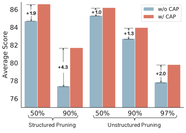
Figure 1: Comparison between BERT pruning with and without Cap. We report the average score across MNLI, QQP, and SQuAD tasks with different model sparsity ($50\%$, $90\%$, and $97\%$). Cap consistently yield improvements for different pruning criterions, with larger gains in higher sparsity $(1.0\rightarrow 1.3\rightarrow 2.0)$. Please refer to Table 2 for details.

Pre-trained Language Models (PLMs), such as BERT (Devlin et al. 2019), have achieved great success in a variety of Natural Language Processing (NLP) tasks. PLMs are pre-trained in a self-supervised way, and then adapted to the downstream tasks through fine-tuning. Despite the success, PLMs are usually resource-hungry with a large number of parameters, ranging from millions (e.g., BERT) to billions (e.g., GPT-3), which leads to high memory consumption and computational overhead in practice.

In fact, recent studies have observed that PLMs are over-parameterized with many redundant weights (Frankle and Carbin 2019; Prasanna, Rogers, and Rumshisky 2020). Motivated by this, one major line of works to compress large-scale PLMs and speed up the inference is model pruning, which focuses on identifying and removing those unimportant parameters. However, when adapting the pre-trained models to downstream tasks, most studies simply adopt the vanilla pruning methods, but do not make full use of the paradigm of pre-training and fine-tuning. Specifically, most works only pay attention to the task-specific knowledge towards the downstream task during pruning, but ignore whether the task-agnostic knowledge of the origin PLM is well maintained in the pruned model. Losing such task-agnostic knowledge can cause severe catastrophic forgetting problem (Lee, Cho, and Kang 2020; Chen et al. 2020a), which further damages the generalization ability of the pruned model. Moreover, when facing extremely high sparsity scenarios (e.g., 97% sparsity with only 3% parameters reserved), the performance of the pruned model decreases sharply compared with the original dense model.

In this paper, we propose Contrastive pruning (Cap), a general pruning framework under the pre-training and fine-tuning paradigm. The core of Cap is to encourage the pruned model to learn from multiple perspectives to reserve different types of knowledge, even in extremely high sparsity scenarios. We adopt contrastive learning (He et al. 2020; Chen et al. 2020b) to achieve the above objective with three modules: PrC, SnC, and FiC. These modules contrast sentence representations derived from the pruned model with those from other models, so that the pruned model is able to learn from others and reserve corresponding representation ability. Specifically, PrC and FiC strive to pull the representation from pruned model towards that from the origin pre-trained model and fine-tuned model, to learn the task-agnostic and task-specific knowledge, respectively. As a bridging mechanism, SnC further strives to pull the representation from pruned model towards that from the intermediate models during pruning (called snapshots), to acquire historical and diversified knowledge, so that the highly sparse model can still maintain comparable performance.

Our Cap framework has the following advantages: 1) Cap maintains both task-agnostic and task-specific knowledge in the pruned model, which helps alleviate catastrophic forgetting problem and maintain model performance during pruning, especially in extremely high sparsity cases; 2) Cap is based on contrastive learning that is proven to be a powerful representation learning technique; 3) Cap is a framework rather than a specific pruning method. Hence, it is orthogonal to various pruning criteria, including both structured and unstructured pruning, and can be flexibly integrated with them to offer improvements.

Cap is conceptually general and empirically powerful. As shown in Figure 1, our experiments show that by equipping different pruning criteria with Cap, the average scores across several tasks are consistently improved by up to $4.3$ point, achieving the state-of-the-art performance among different pruning mechanisms. The improvement even grows larger in higher sparsity. Our experiments also demonstrate that Cap succeeds to achieve $99.2\%$ and $96.3\%$ of the original BERT performance, with only $3\%$ model parameters in QQP and MNLI tasks. Through task transferring probing experiments, we also find that the generalization ability of the pruned model is significantly enhanced with Cap.

Background

Model Compression

Pre-trained Language Models (PLMs) have achieved remarkable success in NLP community, but the demanding memory and latency also greatly increase. Different compression methods, such as model pruning (Han et al. 2015; Molchanov et al. 2017), knowledge distillation (Jiao et al. 2020; Wang et al. 2020), quantization (Shen et al. 2020), and matrix decomposition (Lan et al. 2020), have been proposed.

In this paper, we mainly focus on model pruning, which identifies and removes unimportant weights of the model. It can be divided into two categories, that is, unstructured pruning that prunes individual weights, and structured pruning that prunes structured blocks of weights.

For unstructured pruning, magnitude-based methods prunes weights according to their absolute values (Han et al. 2015; Xu et al. 2021), while movement-based methods consider the change of weights during fine-tuning (Sanh, Wolf, and Rush 2020). In addition, Louizos, Welling, and Kingma (2018) use a hard-concrete distribution to exert L₀-norm regularization, and Guo et al. (2019) introduce reweighted L₁-norm regularization instead.

For structured pruning, some studies use the first-order Taylor expansion to calculate the importance scores of different heads and feed-forward networks based on the variation in the loss if we remove them (Molchanov et al. 2017; Michel, Levy, and Neubig 2019; Prasanna, Rogers, and Rumshisky 2020; Liang et al. 2021). Lin et al. (2020) prune modules whose outputs are very small. Although the above structured pruning methods are matrix-wise, there are also some studies focusing on layer-wise (Fan, Grave, and Joulin 2020; Sajjad et al. 2020), and row/column-wise (Khetan and Karnin 2020; Li et al. 2020).

Different pruning methods can be applied in a one-shot (prune for once) way, or iteratively (prune step by step) that we use in this paper. However, most of the prior methods only consider task-specific knowledge of downstream tasks, but neglect to reserve task-agnostic knowledge in the pruned model, which leads to catastrophic forgetting problem.

Contrastive Learning

Contrastive learning serves as an effective mechanism for representation learning. With similar instances considered as positive examples, and dissimilar instances as negative ones, contrastive learning aims at pulling positive examples close together and pushing negative examples apart, which usually uses InfoNCE loss (van den Oord, Li, and Vinyals 2018). He et al. (2020) and Chen et al. (2020b) propose self-supervised contrastive learning in computer vision, with different views of the figure being positive examples, and different figures being negative examples. It is also successfully introduced to NLP community, such as sentence representation (Wu et al. 2020; Gao, Yao, and Chen 2021), text summarization (Liu and Liu 2021), and so on. In order to take advantage of annotated labels of the data, some studies extend the contrastive learning in a supervised way with an arbitrary number of positive examples (Khosla et al. 2020; Gunel et al. 2021).

Formally, suppose that we have an example $x_{i}$ and it is encoded into a vector representation $z_{i}=\phi(x_{i})\in\mathbb{R}^{d}$ by model $\phi$. Besides, there are also $N$ examples being encoded into $\mathcal{S}=\left\{\hat{z}_{j}\right\}^{N}_{j=1}$, which are used to contrast with $z_{i}$. Suppose there is one or multiple positive examples $\hat{z}_{p}\in\mathcal{S}$ and the others $\mathcal{S}\backslash\left\{\hat{z}_{p}\right\}$ are negative examples towards $z_{i}$. Following Khosla et al. (2020), the contrastive training objective for example $x_{i}$ is defined as follows:

$$\mathcal{L}_{i}=-\frac{1}{\left\|P(i)\right\|}\sum_{\hat{z}_{j}\in P(i)}\log\frac{e^{\mathrm{sim}(z_{i},\hat{z}_{j})/\tau}}{\sum_{k=1}^{N}e^{\mathrm{sim}(z_{i},\hat{z}_{k})/\tau}}$$ (1)

where $P(i)\subset\mathcal{S}$ refers to the positive examples set for $z_{i}$, $\mathrm{sim}(z_{i},z_{j})=\frac{z_{i}^{\top}z_{j}}{\left\|z_{i}\right\|\left\|z_{j}\right\|}$ refers to the cosine similarity function, and $\tau$ denotes the temperature hyperparameter.

Methodology

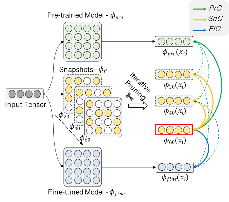
Figure 2: Overview of Cap framework, which prunes model step by step ($\phi_{pre}\rightarrow\phi_{20}\rightarrow\phi_{40}\rightarrow\phi_{60}$), where the number denotes the sparsity ratio (%). Overall, Cap consists of three contrastive modules: PrC, SnC, and FiC. PrC (green lines): contrastive learning with the pre-trained model $\phi_{pre}$ to maintain task-agnostic knowledge. SnC (yellow lines): contrastive learning with snapshots $\phi_{r^{\prime}}$ to bridge the gap between pre-trained model and current pruned model, and gain historic and diversified knowledge. FiC (blue lines): contrastive learning with the fine-tuned model $\phi_{fine}$ to gain the task-specific knowledge. The solid lines indicate the learning of the current pruned model $\phi_{60}$, while the dashed lines denote the learning of previous snapshots, $\phi_{20}$ and $\phi_{40}$.

Module	Supervised	Unsupervised
PrC	$\left\{\phi_{pre}(x_{j})\mid y_{j}=y_{i}\right\}$	$\left\{\phi_{pre}(x_{i})\right\}$
SnC	$\left\{\phi_{r^{\prime}}(x_{j})\mid y_{j}=y_{i},r^{\prime}<r\right\}$	$\left\{\phi_{r^{\prime}}(x_{i})\mid r^{\prime}<r\right\}$
FiC	$\left\{\phi_{fine}(x_{j})\mid y_{j}=y_{i}\right\}$	$\left\{\phi_{fine}(x_{i})\right\}$

Table 1: Positive examples $P(i)$ in Eq. 1 for $\phi_{r}(x_{i})$ in three contrastive modules of Cap. $\phi_{r}(x_{i})$ refers to representation of $x_{i}$ encoded by model $\phi_{r}$ with $r\%$ sparsity ratio, and $y_{i}$ denotes the annotated label for $x_{i}$.

In this paper, we propose a general pruning framework, Contrastive pruning (Cap), which prunes model via supervisions from pre-trained and fine-tuned models, and snapshots during pruning to gain different types of knowledge. Following iterative pruning, we compress the pre-trained model $\phi_{pre}$ to expected sparsity ratio $R\%$ progressively ($\phi_{pre}\rightarrow\phi_{r1}\rightarrow\phi_{r2}\rightarrow\cdots\rightarrow\phi_{R}$), and arbitrary pruning criteria can be used at each step. Figure 2 illustrates the overview of Cap that consists of three modules: PrC, SnC, and FiC. They are all based on contrastive learning, with different ways to construct positive examples shown in Table 1.

PrC: Contrastive Learning with Pre-trained Model

On the transfer learning towards a specific downstream task, the task-agnostic knowledge in the original PLM is inclined to be lost, which can cause catastrophic forgetting problem. Hence, in this section, we introduce a PrC module to maintain such general-purpose language knowledge based on contrastive learning (green lines in Figure 2).

Suppose that example $x_{i}$ is encoded into $z_{i}=\phi_{r}(x_{i})\in\mathbb{R}^{d}$ by model $\phi_{r}$ with $r\%$ sparsity ratio. The high-level idea is that we can contrast $z_{i}$ with $\left\{\hat{z}_{j}=\phi_{pre}(x_{j})\right\}_{j=1}^{N}$ encoded by pre-trained model $\phi_{pre}$ and enforce the model to correctly identify those semantically similar (positive) examples. In this way, the current pruned model $\phi_{r}$ is able to mimic the representation modeling ability of the pre-trained model, and therefore maintain task-agnostic knowledge.

Specifically, we adopt contrastive learning in both unsupervised and supervised settings. For unsupervised PrC, $\phi_{pre}(x_{i})$ is considered as a positive example for $\phi_{r}(x_{i})$, and $\left\{\phi_{pre}(x_{j})\right\}_{j\neq i}$ are negative examples. The loss $\mathcal{L}_{\mathrm{unsup}}^{\mathrm{\emph{PrC}}}$ is then calculated following Eq. 1. For supervised PrC, we further utilize the sentence-level annotations of the data. For example, the sentences are labeled as entailment, neutral, or contradiction in the MNLI task. Intuitively, we treat those having the same labels with $x_{i}$ as positive examples since they share similar semantic features, and the others as negative ones. Formally, we define the positive examples set as $\left\{\phi_{pre}(x_{j})\mid y_{j}=y_{i}\right\}$, where $y_{i}$ denotes the label of $x_{i}$. Then the supervised loss $\mathcal{L}_{\mathrm{sup}}^{\mathrm{\emph{PrC}}}$ is calculated as Eq. 1. Therefore, the final training objective for PrC is $\mathcal{L}^{\mathrm{\emph{PrC}}}=\mathcal{L}_{\mathrm{unsup}}^{\mathrm{\emph{PrC}}}+\mathcal{L}_{\mathrm{sup}}^{\mathrm{\emph{PrC}}}$.

SnC: Contrastive Learning with Snapshots

Pruning can be applied in a one-shot or iterative way. One-shot pruning drops out weights and retrains the model for once. In contrast, iterative pruning removes weights step by step, until reaching the expected sparsity, and the intermediate models at each pruning iterations are called snapshots. In this paper, we adopt iterative pruning since it better suits high sparsity regimes. However, different from prior studies that simply ignore these snapshots, we propose SnC to enable the current pruned model to learn from these snapshots based on contrastive learning (yellow lines in Figure 2).

In detail, suppose that we prune the model to $r\%$ sparsity ratio progressively ($\phi_{pre}\rightarrow\phi_{r1}\rightarrow\phi_{r2}\rightarrow\cdots\rightarrow\phi_{r}$), and $\left\{\phi_{r^{\prime}}\right\}_{r^{\prime}<r}=\left\{\phi_{r1},\phi_{r2},\dots\right\}$ are snapshots. Intuitively, these snapshots can bridge the gap between the sparse model ($\phi_{r}$) and dense models ($\phi_{pre}$, $\phi_{fine}$), and provide diversified supervisions with different sparse structures. Under unsupervised settings, for example $x_{i}$ encoded into $\phi_{r}(x_{i})\in\mathbb{R}^{d}$ by the current pruned model $\phi_{r}$, we treat the representations encoded from the same example but by the snapshots $\left\{\phi_{r^{\prime}}(x_{i})\mid r^{\prime}<r\right\}$ as positive examples, and $\left\{\phi_{r^{\prime}}(x_{j})\mid j\neq i,r^{\prime}<r\right\}$ as negative ones. Under supervised settings, we utilize the annotation labels to consider instances with the same labels as positive examples. We calculate the loss for SnC following Eq. 1, $\mathcal{L}^{\mathrm{\emph{SnC}}}=\mathcal{L}_{\mathrm{unsup}}^{\mathrm{\emph{SnC}}}+\mathcal{L}_{\mathrm{sup}}^{\mathrm{\emph{SnC}}}$. Table 3 show that snapshots serve as effective guidance during pruning, with $0.58\sim 2.47$ average gains on MNLI, QQP, and SQuAD, especially in high sparsity regimes.

FiC: Contrastive Learning with Fine-tuned Model

To better adapt to the downstream task, the pruned model $\phi_{r}$ can also learn from the fine-tuned model $\phi_{fine}$ that contains rich task-specific knowledge. To this end, we propose a FiC module, which conducts contrastive learning between the current pruned model $\phi_{r}$ and the fine-tuned model $\phi_{fine}$. It is almost identical to the PrC module, except that the target model $\phi_{pre}$ is replaced with the fine-tuned model $\phi_{fine}$ (blue lines in Figure 2). Accordingly, the training loss is calculated as $\mathcal{L}^{\mathrm{\emph{FiC}}}=\mathcal{L}_{\mathrm{unsup}}^{\mathrm{\emph{FiC}}}+\mathcal{L}_{\mathrm{sup}}^{\mathrm{\emph{FiC}}}$ based on Eq. 1. In addition to the contrastive supervision signal in representation space, we can also introduce distilling supervision in label space through knowledge distillation mechanism.

Pruning with Cap Framework

Putting PrC, SnC, and FiC together, we can reach our proposed Cap framework. Note that we can flexibly integrate with different pruning criteria in Cap. In this paper, we try out both structured and unstructured pruning criteria.

For structured pruning, a widely used structured pruning criterion is to derive the importance score of an element based on the variation towards the loss $\mathcal{L}$ if we remove it, using the first-order Taylor expansion (Molchanov et al. 2017) of the loss. We denote this method as First-order pruning and absorb it into Cap, which we call Cap-f.

$$I_{w}=\left|\mathcal{L}_{w}-\mathcal{L}_{w=0}\right|\approx\left|\frac{\partial\mathcal{L}}{\partial w}w\right|$$ (2)

For unstructured pruning, we apply the movement-based pruning methods (Sanh, Wolf, and Rush 2020), which calculates importance score for parameter $w$ as follows:

$$I_{w}=-\sum_{t}\frac{\partial\mathcal{L}^{(t)}}{\partial w}w^{(t)}$$ (3)

where $t$ is the training step. Based on it, Sanh, Wolf, and Rush (2020) reserve parameters using Top-K selection strategy or a pre-defined threshold, called Movement pruning or Soft-movement pruning, respectively. We absorb these methods into Cap, and denote them as Cap-m and Cap-soft.

Finally, we prune and train the model using the final objective $\mathcal{L}=\lambda_{1}\mathcal{L}^{CE}+\lambda_{2}\mathcal{L}^{PrC}+\lambda_{3}\mathcal{L}^{SnC}+\lambda_{4}\mathcal{L}^{FiC}$, where $\mathcal{L}^{CE}$ is the cross-entropy loss towards the downstream task.

Extra Memory Overhead

In our proposed Cap framework, the pruned model learns from the pre-trained, snapshots, and fine-tuned models. However, there is unnecessary to load all of these models in GPU, which can lead to large GPU memory overhead. In fact, because only the sentence representations of examples are required for Eq. 1 in contrastive learning, and they also do not back-propagate the gradients, we can simply pre-encode the examples and store them in CPU. When a normal input batch arrives, we fetch $N$ pre-encoded examples for contrastive learning. In our paper, we use $N=4096$ by default, and the dimensions of the sentence representation for BERT_base are $768$. Therefore, the extra GPU memory overhead is $4096\times 768=3.15$M in total, and only takes up $3.15$M / $110$M = $2.86\%$ of the memory consumption of BERT_base, which is low enough and acceptable.

Experiments

Datasets

We conduct experiments on various tasks to illustrate the effectiveness of Cap, including a) MNLI, the Multi-Genre Natural Language Inference Corpus (Williams, Nangia, and Bowman 2018), a natural language inference task with in-domain test set (MNLI-m), and cross-domain one (MNLI-mm). b) QQP, the Quora Question Pairs dataset (Wang et al. 2019), a pairwise semantic equivalence task. c) SST-2, the Stanford Sentiment Treebank (Socher et al. 2013), a sentiment classification task for an individual sentence. d) SQuAD v1.1, the Stanford Question Answering Dataset (Rajpurkar et al. 2016), an extractive question answering task with crowdsourced question-answer pairs. Following most prior works (Lin et al. 2020; Sanh, Wolf, and Rush 2020), we report results for the dev sets. The detailed statistics and the metrics are provided in Appendix.

Experiment Setups

We conduct experiments based on BERT_base (Devlin et al. 2019) with $110$M parameters, and follow their settings unless noted otherwise. Following Sanh, Wolf, and Rush (2020), we prune and report the sparsity ratio based on the weights of the encoder. For Cap-f, we prune $10\%$ parameters each step and retrain the model to recover the performance until reaching the expected sparsity. For Cap-m and Cap-soft, we follow the cubic sparsity scheduling with cool-down strategy and hyperparameter settings the same as  Sanh, Wolf, and Rush (2020). The number of examples for contrastive learning is $N=4096$. We use the final hidden state of $[CLS]$ as the sentence representation, which is shown to be slightly better than mean pooling in our exploration experiments. We search the temperature from $\tau=\left\{0.05,0.1,0.2,0.3\right\}$.

Main Results

Methods	Sparsity	MNLI-m/-mm	QQPACC/F1	SST-2	SQuADEM/F1
BERTbase	0%	84.5x/x84.4	90.9x/x88.0	92.9	80.7x/x88.4
Knowledge Distillation
DistillBERT (Sanh et al. 2019)	50%	82.2x/xxx-x	88.5x/xxx-x	91.3	78.1x/x86.2
BERT-PKD (Sun et al. 2019)	50%	xx-xx/x81.0	88.9x/xxx-x	91.5	77.1x/x85.3
TinyBERT (Jiao et al. 2020)	50%	83.5x/xxx-x	90.6x/xxx-x	91.6	79.7x/x87.5
MiniLM (Wang et al. 2020)	50%	84.0x/xxx-x	91.0x/xxx-x	92.0	xx-xx/xxx-x
TinyBERT (Jiao et al. 2020)	66.7%	80.5x/x81.0	xx-xx/xxx-x	-	72.7x/x82.1
Structured Pruning
First-order (Molchanov et al. 2017)	50%	83.2x/x83.6	90.8x/x87.5	90.6	77.2x/x86.0
Top-drop (Sajjad et al. 2020)	50%	81.1x/xxx-x	90.4x/xxx-x	90.3	xx-xx/xxx-x
SNIP (Lin et al. 2020)	50%	xx-xx/x82.8	88.9x/xxx-x	91.8	xx-xx/xxx-x
schuBERT (Khetan and Karnin 2020)	50%	83.8x/xxx-x	xx-xx/xxx-x	91.7	80.7x/x88.1
Cap-f (Ours)	50%	84.5x/x85.0	91.6x/x88.6	92.7	81.4x/x88.7
SNIP (Lin et al. 2020)	75%	xx-xx/x78.3	87.8x/xxx-x	88.4	xx-xx/xxx-x
First-order (Molchanov et al. 2017)	90%	79.1x/x79.5	88.7x/x84.9	86.9	59.8x/x72.3
Cap-f (Ours)	90%	81.0x/x81.2	90.2x/x86.9	89.7	70.2x/x80.6
Unstructured Pruning
Movement (Sanh, Wolf, and Rush 2020)	50%	82.5x/x82.9	91.0x/x87.8	-	79.8x/x87.6
Cap-m (Ours)	50%	83.8x/x84.2	91.6x/x88.6	-	80.9x/x88.2
Magnitude (Han et al. 2015)	90%	78.3x/x79.3	79.8x/x65.0	-	70.2x/x80.1
L0-regularization (Louizos, Welling, and Kingma 2018)	90%	78.7x/x79.7	88.1x/x82.8	-	72.4x/x81.9
Movement (Sanh, Wolf, and Rush 2020)	90%	80.1x/x80.4	89.7x/x86.2	-	75.6x/x84.3
Soft-Movement (Sanh, Wolf, and Rush 2020)	90%	81.2x/x81.8	90.2x/x86.8	-	76.6x/x84.9
Cap-m (Ours)	90%	81.1x/x81.8	91.6x/x87.7	-	76.5x/x85.1
Cap-soft (Ours)	90%	82.0x/x82.9	90.7x/x87.4	-	77.1x/x85.6
Movement (Sanh, Wolf, and Rush 2020)	97%	76.5x/x77.4	86.1x/x81.5	-	67.5x/x78.0
Soft-Movement (Sanh, Wolf, and Rush 2020)	97%	79.5x/x80.1	89.1x/x85.5	-	72.7x/x82.3
Cap-m (Ours)	97%	77.5x/x78.4	88.8x/x85.0	-	69.5x/x79.7
Cap-soft (Ours)	97%	80.1x/x81.3	90.2x/x86.7	-	73.8x/x83.0

Table 2: Comparison between Cap with other model compression methods without data augmentation. Cap consistently achieve the best performance under the same sparsity ratio across different tasks. With only $3\%$ of the encoder’s parameter (i.e., 97% sparsity), Cap-soft still reaches $99.2\%$ and $96.3\%$ of the original BERT performance in QQP and MNLI task, respectively.

In this section, we compare Cap with the following model compression methods: 1) knowledge distillation: DistillBERT (Sanh et al. 2019), BERT-PKD (Sun et al. 2019), TinyBERT (Jiao et al. 2020), and MiniLM (Wang et al. 2020). Note that we report the results of TinyBERT without data augmentation mechanism to ensure fairness. 2) structured pruning: the most standard First-order pruning (Molchanov et al. 2017) that Cap-f is based, Top-drop (Sajjad et al. 2020), SNIP (Lin et al. 2020), and schuBERT (Khetan and Karnin 2020). 3) unstructured pruning: Magnitude pruning (Han et al. 2015), L₀-regularization (Louizos, Welling, and Kingma 2018), and the state-of-the-art Movement pruning and Soft-movement pruning (Sanh, Wolf, and Rush 2020) that our Cap-m and Cap-soft are based on. Please refer to the Appendix for more details about the baselines. Table 2 illustrates the main results, from which we have some important observations.

(1) Cap removes a large proportion of BERT parameters while still maintaining comparable performance. With $50\%$ sparsity ratio, Cap-f achieves an equal score in MNLI-m compared with origin BERT, and even improves by $0.3\sim 0.7$ score for MNLI-mm, QQP, and SQuAD tasks. More importantly, with only $3\%$ of the encoder’s parameters (i.e., $97\%$ sparsity ratio), our Cap-soft successfully achieves $99.2\%$ and $96.3\%$ of the original BERT performance in QQP ($90.9\rightarrow 90.2$) and MNLI-mm ($84.4\rightarrow 81.3$).

(2) Cap consistently yields improvements for different pruning criteria, along with larger gains in higher sparsity. Compared with structured First-order pruning, Cap-f improves by $1.9(85.6\rightarrow 87.5)$ and $4.1(78.7\rightarrow 82.8)$ average score over all tasks under $50\%$ and $90\%$ sparsity. Similarly, compared with unstructured Movement pruning, as the sparsity grows by $50\%\rightarrow 90\%\rightarrow 97\%$, Cap-m improves $1.0(85.2\rightarrow 86.2)$, $1.3(82.7\rightarrow 84.0)$, and $2.0(77.8\rightarrow 79.8)$ scores, which also increases accordingly.

(3) Cap consistently outperforms other pruning methods. For example, Cap-f surpasses SNIP by $2.2$ and $2.7$ score in MNLI-mm and QQP tasks under $50\%$ sparsity. Besides, with higher sparsity, the $90\%$-sparsified Cap-f can even beat SNIP with $75\%$ sparsity, with $2.9$ and $2.4$ higher score in the MNLI-mm and QQP tasks.

(4) Cap also outperforms knowledge distillation methods. For example, compared with TinyBERT under $66.7\%$ sparsity ratio, Cap-f that is under $90\%$ sparsity ratio can still surpass it by $0.5$ accuracy in the MNLI-m task.

The above observations support our claim that Cap helps the pruned model to maintain both task-agnostic and task-specific knowledge and hence benefits the pruning, especially under extremely high sparsity scenarios.

Generalization Ability

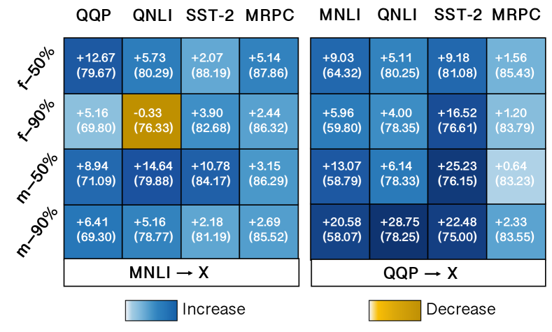
Figure 3: Generalization ability probing. We transfer the pruned model trained on MNLI (left) and QQP (right) to target tasks under $50\%$ and $90\%$ sparsity ratio. We report the improvement brought by Cap compared with its basic pruning method, and the absolute performance of Cap (in bracket). Cap yields improvement in most cases, suggesting better generalization ability of the model pruned by Cap.

Different from prior methods, Cap can maintain task-agnostic knowledge in the pruned model, and therefore strengthen its generalization ability. To justify our claim, we follow the task transfer probing experiments from  Aghajanyan et al. (2021). In detail, we freeze the representations derived from the pruned model trained on MNLI or QQP, and then only train a linear classifier on top of the model for another task. Besides MNLI, QQP, and SST-2 tasks we have used, we also include QNLI (Wang et al. 2019) and MRPC (Dolan and Brockett 2005) as our target tasks.

The results under $50\%$ and $90\%$ sparsity are shown in Figure 3, where the first two rows correspond to the improvement of Cap-f over First-order pruning, and the last two rows correspond to the improvement of Cap-m over Movement pruning. Improvements are shown at each cell, with the performance score of Cap in the bracket. As is shown, Cap yields improvements in an overwhelming majority of cases. For example, Cap-m outperforms Movement pruning by a large margin, with up to $28.75$ higher score in QNLI transferred from QQP task, under $90\%$ sparsity. The significant improvements in task transferring experiments suggest Cap can better maintain the task-agnostic knowledge and strengthen the generalization ability of the pruned model.

Discussions

Understanding Different Contrastive Modules

Methods	Sparsity	MNLI-m	QQP	SQuAD	$\bf\Delta$
Cap-f	50%	84.48	88.49	81.37	-
- w/o PrC		-0.47	-0.50	-0.67	-0.55
- w/o SnC		-0.47	-0.57	-1.10	-0.71
- w/o FiC		-0.42	-0.63	-0.58	-0.54
Cap-f	90%	80.98	86.92	70.16	-
- w/o PrC		-1.78	-0.87	-5.11	-2.59
- w/o SnC		-1.57	-1.72	-4.11	-2.47
- w/o FiC		-1.53	-1.31	-2.64	-1.83
Cap-m	50%	83.29	88.28	80.40	-
- w/o PrC		-0.84	-0.22	-0.74	-0.60
- w/o SnC		-0.74	-0.36	-0.66	-0.59
- w/o FiC		-1.31	-0.77	-1.07	-1.05
Cap-m	90%	80.53	87.12	76.20	-
- w/o PrC		-0.58	-0.47	-0.68	-0.58
- w/o SnC		-0.45	-0.78	-0.66	-0.58
- w/o FiC		-1.54	-0.73	-0.94	-1.07
Cap-m	97%	77.30	84.70	69.47	-
- w/o PrC		-0.27	-0.23	-1.87	-0.79
- w/o SnC		-0.29	-0.52	-1.67	-0.83
- w/o FiC		-1.31	-0.34	-2.11	-1.25

Table 3: Ablation study of different contrastive modules. $\Delta$ refers to the average score reduction across all tasks. Removing any contrastive module would cause degradation of the pruned model, especially in highly sparse regimes.

Cap is mainly comprised of three major contrastive modules, PrC for learning from the pre-trained model, SnC for learning from snapshots, and FiC for learning from the fine-tuned model. To better explore their effects, we remove one of them from Cap at a time, and prunes model with Cap-f and Cap-m methods under various sparsity ratios.

We report the accuracy for MNLI-m, F1 for QQP, and Exact Match score for SQuAD, along with the average score decrease $\Delta$. As shown in Table 3, removing any contrastive module would cause degradation of the model. For example, with $90\%$ sparsity ratio, removing PrC, SnC, or FiC leads to $1.83\sim 2.59$ average score reduction for Cap-f, and $0.58\sim 1.07$ for Cap-m. Besides, the performance degradation gets larger as the sparsity gets higher in general. This is especially evident for Cap-f. For instance, using Cap-f without PrC module, when the sparsity ratio varies from $50\%$ to $90\%$, the degradation increases from $0.55$ to $2.59$, The results demonstrate that all contrastive modules play important roles in Cap, and have complementary advantages with each other, especially in highly sparse regimes.

Understanding Supervised and Unsupervised Contrastive Objectives

Methods	Sparsity	MNLI-m/-mm	QQPACC/F1	$\bf\Delta$
Cap-f	50%	84.48x/x84.97	91.45x/x88.49	-
- w/o sup		-0.64x/x-0.30	-0.53xx/-0.65	-0.53
- w/o unsup		-0.47x/x-0.24	-0.56x/x-0.69	-0.49
Cap-f	90%	80.98x/x81.17	90.23x/x86.92	-
- w/o sup		-0.97x/x-0.69	-0.84x/x-0.99	-0.87
- w/o unsup		-1.29x/x-1.03	-0.85x/x-1.19	-1.09
Cap-m	50%	83.29x/x83.91	91.34x/x88.28	-
- w/o sup		-0.80x/x-0.76	-0.37x/x-0.47	-0.60
- w/o unsup		-0.86x/x-0.53	-0.48x/x-0.63	-0.63
Cap-m	90%	80.53x/x81.13	90.44x/x87.12	-
- w/o sup		-0.71x/x-0.85	-1.36x/x-0.70	-0.91
- w/o unsup		-0.91x/x-1.18	-1.62x/x-1.29	-1.25
Cap-m	97%	77.30x/x78.21	88.56x/x84.7	-
- w/o sup		-0.36x/x-0.43	-0.95x/x-1.52	-0.82
- w/o unsup		-0.39x/x-0.58	-0.80x/x-1.02	-0.70

Table 4: Ablation study of supervised (sup) and unsupervised (unsup) training objectives. $\Delta$ is the average score reduction across all scores. Both supervised and unsupervised contrastive learning objectives are beneficial to the pruning, and combining them can lead to better performance.

In Cap, the same example encoded by different models are considered as positive examples for unsupervised contrastive learning (unsup). If the sentence-level label annotations are available, we can also conduct supervised contrastive learning (sup) by considering examples with the same labels as positive examples. To explore their effects, we remove either of them for the ablation study.

As demonstrated in Table 4, without either supervised or unsupervised contrastive learning objectives, the performance of the pruned model would markedly decline. Specifically, removing the supervised contrastive learning objective leads to $0.53\sim 0.91$ average score decrease for Cap, while abandoning the unsupervised one also causes $0.49\sim 1.25$ decrease. It suggests that both supervised and unsupervised objectives are essential and necessary for Cap, and their advantages are orthogonal to each other.

Performance under Various Sparsity Ratios

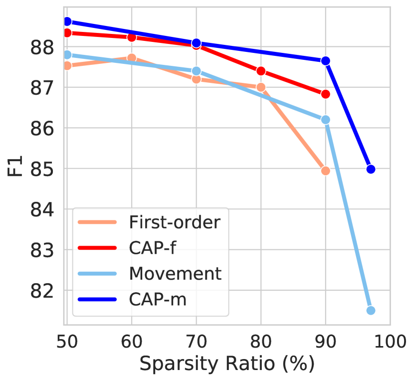
(a) QQP

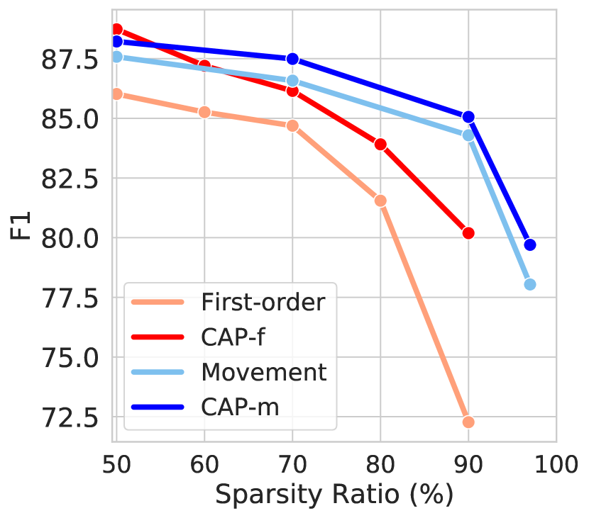
(b) SQuAD

Figure 4: Comparison between Cap and its basic pruning methods. Cap-f consistently outperforms First-order pruning, and Cap-m also surpasses Movement pruning under various sparsity ratios.

In this section, we compare Cap-f and Cap-m with their basic pruning methods, First-order pruning and Movement pruning, with sparsity ratios varying from $50\%$ to $97\%$. The evolution of the performance in QQP and SQuAD task is shown in Figure 4. The performance of the pruned model for all methods decreases as the sparsity ratio increases. However, we can observe that Cap-f consistently outperforms First-order pruning, and the improvement is even larger in higher sparsity situations. A similar tendency also exists between Cap-m and Movement pruning. These results suggest that with three core contrastive modules, Cap can better maintain the model performance during the pruning.

Exploration of Pooling Methods and Temperatures

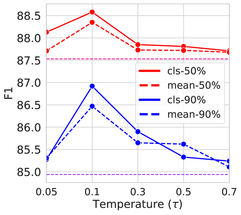
(a) Cap-f

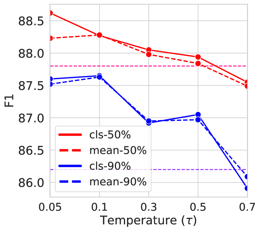
(b) Cap-m

Figure 5: Performance of different pooling methods and temperatures. The horizontal dashed line denotes the performance of First-order and Movement pruning under $50\%$ and $90\%$ sparsity. In general, using $[CLS]$ as sentence representations slightly outperforms mean pooling, and temperature $\tau=0.1$ tends to achieve the best results.

The contrastive loss function in Eq. 1 involves two important points, the sentence representation $z_{i}$ and the temperature $\tau$. For sentence representation $z_{i}$, we explore two pooling methods of the hidden states encoded by the model, using the vector representation of the $[CLS]$ or the mean pooling of all representations of the whole sentence. For temperature $\tau$, we also explore different values ranging from $0.05$ to $0.7$. We conduct experiments on QQP. As shown in Figure 5, using $[CLS]$ as sentence representations slightly outperforms the mean pooling method. Besides, Cap can achieve better performance than its basic pruning method under most temperatures, and setting $\tau=0.1$ tends to achieve the best performance in most cases.

Exploration of Learning From Fine-tuned Model

Methods	QQP		SQuAD
	50%	90%	50%	90%
Movement	87.80	86.20	87.58	84.29
- w/o KD	87.30	83.20	83.16	81.72
Cap-f	88.58	86.92	88.73	80.59
- w/o KD	88.59	86.88	86.52	77.76
Cap-m	88.62	87.65	88.22	85.06
- w/o KD	88.60	87.67	85.94	82.46

Table 5: Exploring of learning from the fine-tuned model. For Cap, KD brings improvements for token-level task (SQuAD), but has little effect on sentence-level task (QQP).

To gain task-specific knowledge, we propose to perform contrastive learning on the sentence representations from the fine-tuned model (FiC). Another common way is to perform the knowledge distillation (KD) on the soft label that has already been shown effective in pruning (Sanh, Wolf, and Rush 2020; Hou et al. 2020). To explore the effect of KD, we conduct further experiments in Table 5. It shows that KD boosts the performance of CAP in token-level task (SQuAD) while has little effect on sentence-level task (QQP). The reason can be that the contrastive learning on the sentence representations is sufficient to capture the features of the sentence-level task, while the information still incurs losses on token-level tasks. Thus, for token-level tasks, it is better to perform Cap with KD.

Conclusion

In this paper, we propose a general pruning framework, Contrastive pruning (Cap), under the paradigm of pre-training and fine-tuning. Based on contrastive learning, we enhance the pruned model to maintain both task-agnostic and task-specific knowledge via pulling it towards the representations from the pre-trained model $\phi_{pre}$, and fine-tuned model $\phi_{fine}$. Furthermore, the snapshots during the pruning process are also fully utilized to provide historic and diversified supervisions to retain the performance of the pruned model, especially in high sparsity regimes. Cap consistently yields significant improvements to different pruning criteria, and achieves the state-of-the-art performance among different pruning mechanisms. Experiments also show that Cap strengthen the generalization ability of the pruned model.

Datasets and Metrics

The detailed statistics of different datasets are shown in Table 6. The metrics we report for each dataset are also illustrated in Table 6. We obtain the data from https://huggingface.co/datasets/glue.

Dataset	#Train	#Dev	Metrics
MNLI-m	393k	9.8k	Accuracy
MNLI-mm	393k	9.8k	Accuracy
QQP	364k	40k	Accuracy/F1
SST-2	67k	872	Accuracy
SQuAD	88K	11k	Exact Match/F1

Table 6: Statistics and metrics of datasets used in this paper.

Baseline Compression Methods

We compare with the following compression methods.

Knowledge Distillation

• DistillBERT (Sanh et al. 2019), which distills the soft label on the downstream task predicted by the teacher model towards the student model.

• BERT-PKD (Sun et al. 2019), which also distills the hidden states of the teacher model towards the student models in representation space.

• TinyBERT (Jiao et al. 2020), which distills the hidden states and soft labels from teachers towards student models in both pre-training and fine-tuning phrases.

• MiniLM (Wang et al. 2020), which distills the self-attention module of the last Transformer layer of the teacher towards the student models.

Structured Pruning

• First-order pruning (Molchanov et al. 2017), which uses the first-order Taylor expansion of the loss towards attention heads or feed forward neurons to calculate the importance scores.

• Top-drop (Sajjad et al. 2020), which finds it effective to directly discard the top layers of the BERT and fine-tune on the downstream tasks.

• SNIP (Lin et al. 2020), which prunes modules based on the absolute magnitude of their activation outputs, and introduces a spectral normalization mechanism to stabilize the distribution of the post-activation values of the Transformer layers.

• schuBERT (Khetan and Karnin 2020), which parameterizes each layer of BERT by five different dimensions, and then pre-train BERT with pruning-based criterions to remove the rows or columns of the parameter matrices of BERT.

Unstructured Pruning

• Magnitude pruning (Han et al. 2015), which removes parameters simply accroding to their absolute values.

• L₀-regularization (Louizos, Welling, and Kingma 2018), which sparsifies the model using hard-concrete distribution to exert L₀ regularization.

• Movement pruning (Sanh, Wolf, and Rush 2020), which calculates importance score using Eq. 3 in the main content of the paper, and maintains the Top-K parameters.

• Soft-movement pruning (Sanh, Wolf, and Rush 2020), which is also based on Eq. 3 but maintain parameters according to a threshold.

References

- Aghajanyan et al. (2021) Aghajanyan, A.; Shrivastava, A.; Gupta, A.; Goyal, N.; Zettlemoyer, L.; and Gupta, S. 2021. Better Fine-Tuning by Reducing Representational Collapse. In International Conference on Learning Representations (ICLR).
- Chen et al. (2020a) Chen, S.; Hou, Y.; Cui, Y.; Che, W.; Liu, T.; and Yu, X. 2020a. Recall and Learn: Fine-tuning Deep Pretrained Language Models with Less Forgetting. In Proceedings of the 2020 Conference on Empirical Methods in Natural Language Processing (EMNLP).
- Chen et al. (2020b) Chen, T.; Kornblith, S.; Norouzi, M.; and Hinton, G. 2020b. A Simple Framework for Contrastive Learning of Visual Representations. In Proceedings of the 37th International Conference on Machine Learning (ICML).
- Devlin et al. (2019) Devlin, J.; Chang, M.-W.; Lee, K.; and Toutanova, K. 2019. BERT: Pre-training of Deep Bidirectional Transformers for Language Understanding. In Proceedings of the 2019 Conference of the North American Chapter of the Association for Computational Linguistics (NAACL).
- Dolan and Brockett (2005) Dolan, W. B.; and Brockett, C. 2005. Automatically Constructing a Corpus of Sentential Paraphrases. In Proceedings of the Third International Workshop on Paraphrasing (IWP).
- Fan, Grave, and Joulin (2020) Fan, A.; Grave, E.; and Joulin, A. 2020. Reducing Transformer Depth on Demand with Structured Dropout. In International Conference on Learning Representations (ICLR).
- Frankle and Carbin (2019) Frankle, J.; and Carbin, M. 2019. The Lottery Ticket Hypothesis: Finding Sparse, Trainable Neural Networks. In International Conference on Learning Representations (ICLR).
- Gao, Yao, and Chen (2021) Gao, T.; Yao, X.; and Chen, D. 2021. SimCSE: Simple Contrastive Learning of Sentence Embeddings. arXiv, arXiv:2104.08821.
- Gunel et al. (2021) Gunel, B.; Du, J.; Conneau, A.; and Stoyanov, V. 2021. Supervised Contrastive Learning for Pre-trained Language Model Fine-tuning. In International Conference on Learning Representations (ICLR).
- Guo et al. (2019) Guo, F.; Liu, S.; Mungall, F. S.; Lin, X.; and Wang, Y. 2019. Reweighted Proximal Pruning for Large-Scale Language Representation. arXiv, arXiv:1909.12486.
- Han et al. (2015) Han, S.; Pool, J.; Tran, J.; and Dally, W. 2015. Learning both Weights and Connections for Efficient Neural Network. In Advances in Neural Information Processing Systems (NeurIPS).
- He et al. (2020) He, K.; Fan, H.; Wu, Y.; Xie, S.; and Girshick, R. 2020. Momentum Contrast for Unsupervised Visual Representation Learning. In Proceedings of the IEEE/CVF Conference on Computer Vision and Pattern Recognition (CVPR).
- Hou et al. (2020) Hou, L.; Huang, Z.; Shang, L.; Jiang, X.; Chen, X.; and Liu, Q. 2020. DynaBERT: Dynamic BERT with Adaptive Width and Depth. In Advances in Neural Information Processing Systems (NeurIPS).
- Jiao et al. (2020) Jiao, X.; Yin, Y.; Shang, L.; Jiang, X.; Chen, X.; Li, L.; Wang, F.; and Liu, Q. 2020. TinyBERT: Distilling BERT for Natural Language Understanding. In Findings of the Association for Computational Linguistics: EMNLP 2020.
- Khetan and Karnin (2020) Khetan, A.; and Karnin, Z. 2020. schuBERT: Optimizing Elements of BERT. In Proceedings of the 58th Annual Meeting of the Association for Computational Linguistics (ACL).
- Khosla et al. (2020) Khosla, P.; Teterwak, P.; Wang, C.; Sarna, A.; Tian, Y.; Isola, P.; Maschinot, A.; Liu, C.; and Krishnan, D. 2020. Supervised Contrastive Learning. In Advances in Neural Information Processing Systems (NeurIPS).
- Lan et al. (2020) Lan, Z.; Chen, M.; Goodman, S.; Gimpel, K.; Sharma, P.; and Soricut, R. 2020. ALBERT: A Lite BERT for Self-supervised Learning of Language Representations. In International Conference on Learning Representations (ICLR).
- Lee, Cho, and Kang (2020) Lee, C.; Cho, K.; and Kang, W. 2020. Mixout: Effective Regularization to Finetune Large-scale Pretrained Language Models. In International Conference on Learning Representations (ICLR).
- Li et al. (2020) Li, B.; Kong, Z.; Zhang, T.; Li, J.; Li, Z.; Liu, H.; and Ding, C. 2020. Efficient Transformer-based Large Scale Language Representations using Hardware-friendly Block Structured Pruning. In Findings of the Association for Computational Linguistics: EMNLP 2020.
- Liang et al. (2021) Liang, C.; Zuo, S.; Chen, M.; Jiang, H.; Liu, X.; He, P.; Zhao, T.; and Chen, W. 2021. Super Tickets in Pre-Trained Language Models: From Model Compression to Improving Generalization. In Proceedings of the 59th Annual Meeting of the Association for Computational Linguistics and the 11th International Joint Conference on Natural Language Processing (ACL).
- Lin et al. (2020) Lin, Z.; Liu, J.; Yang, Z.; Hua, N.; and Roth, D. 2020. Pruning Redundant Mappings in Transformer Models via Spectral-Normalized Identity Prior. In Findings of the Association for Computational Linguistics: EMNLP 2020.
- Liu and Liu (2021) Liu, Y.; and Liu, P. 2021. SimCLS: A Simple Framework for Contrastive Learning of Abstractive Summarization. In Proceedings of the 59th Annual Meeting of the Association for Computational Linguistics and the 11th International Joint Conference on Natural Language Processing (ACL).
- Louizos, Welling, and Kingma (2018) Louizos, C.; Welling, M.; and Kingma, D. P. 2018. Learning Sparse Neural Networks through L0 Regularization. In International Conference on Learning Representations (ICLR).
- Michel, Levy, and Neubig (2019) Michel, P.; Levy, O.; and Neubig, G. 2019. Are Sixteen Heads Really Better than One? In Advances in Neural Information Processing Systems (NeurIPS).
- Molchanov et al. (2017) Molchanov, P.; Tyree, S.; Karras, T.; Aila, T.; and Kautz, J. 2017. Pruning Convolutional Neural Networks for Resource Efficient Inference. In International Conference on Learning Representations (ICLR).
- Prasanna, Rogers, and Rumshisky (2020) Prasanna, S.; Rogers, A.; and Rumshisky, A. 2020. When BERT Plays the Lottery, All Tickets Are Winning. In Proceedings of the 2020 Conference on Empirical Methods in Natural Language Processing (EMNLP).
- Rajpurkar et al. (2016) Rajpurkar, P.; Zhang, J.; Lopyrev, K.; and Liang, P. 2016. SQuAD: 100,000+ Questions for Machine Comprehension of Text. In Proceedings of the 2016 Conference on Empirical Methods in Natural Language Processing (EMNLP), 2383–2392.
- Sajjad et al. (2020) Sajjad, H.; Dalvi, F.; Durrani, N.; and Nakov, P. 2020. Poor Man’s BERT: Smaller and Faster Transformer Models. arXiv, abXiv:2004.03844.
- Sanh et al. (2019) Sanh, V.; Debut, L.; Chaumond, J.; and Wolf, T. 2019. DistilBERT, a distilled version of BERT: smaller, faster, cheaper and lighter. arXiv, arXiv:1910.01108.
- Sanh, Wolf, and Rush (2020) Sanh, V.; Wolf, T.; and Rush, A. 2020. Movement Pruning: Adaptive Sparsity by Fine-Tuning. In Advances in Neural Information Processing Systems (NeurIPS).
- Shen et al. (2020) Shen, S.; Dong, Z.; Ye, J.; Ma, L.; Yao, Z.; Gholami, A.; Mahoney, M. W.; and Keutzer, K. 2020. Q-BERT: Hessian Based Ultra Low Precision Quantization of BERT. Proceedings of the AAAI Conference on Artificial Intelligence (AAAI).
- Socher et al. (2013) Socher, R.; Perelygin, A.; Wu, J.; Chuang, J.; Manning, C. D.; Ng, A.; and Potts, C. 2013. Recursive Deep Models for Semantic Compositionality Over a Sentiment Treebank. In Proceedings of the 2013 Conference on Empirical Methods in Natural Language Processing (EMNLP).
- Sun et al. (2019) Sun, S.; Cheng, Y.; Gan, Z.; and Liu, J. 2019. Patient Knowledge Distillation for BERT Model Compression. In Proceedings of the 2019 Conference on Empirical Methods in Natural Language Processing (EMNLP).
- van den Oord, Li, and Vinyals (2018) van den Oord, A.; Li, Y.; and Vinyals, O. 2018. Representation Learning with Contrastive Predictive Coding. arXiv, arXiv:1807.03748.
- Wang et al. (2019) Wang, A.; Singh, A.; Michael, J.; Hill, F.; Levy, O.; and Bowman, S. R. 2019. GLUE: A Multi-Task Benchmark and Analysis Platform for Natural Language Understanding. In International Conference on Learning Representations (ICLR).
- Wang et al. (2020) Wang, W.; Wei, F.; Dong, L.; Bao, H.; Yang, N.; and Zhou, M. 2020. MiniLM: Deep Self-Attention Distillation for Task-Agnostic Compression of Pre-Trained Transformers. In Advances in Neural Information Processing Systems (NeurIPS).
- Williams, Nangia, and Bowman (2018) Williams, A.; Nangia, N.; and Bowman, S. 2018. A Broad-Coverage Challenge Corpus for Sentence Understanding through Inference. In Proceedings of the 2018 Conference of the North American Chapter of the Association for Computational Linguistics (NAACL).
- Wu et al. (2020) Wu, Z.; Wang, S.; Gu, J.; Khabsa, M.; Sun, F.; and Ma, H. 2020. CLEAR: Contrastive Learning for Sentence Representation. arXiv, arXiv:2012.15466.
- Xu et al. (2021) Xu, D.; Yen, I. E.-H.; Zhao, J.; and Xiao, Z. 2021. Rethinking Network Pruning – under the Pre-train and Fine-tune Paradigm. In Proceedings of the 2021 Conference of the North American Chapter of the Association for Computational Linguistics (NAACL).