A New Perspective on the Effects of Spectrum in Graph Neural Networks

Abstract

Many improvements on GNNs can be deemed as operations on the spectrum of the underlying graph matrix, which motivates us to directly study the characteristics of the spectrum and their effects on GNN performance. By generalizing most existing GNN architectures, we show that the correlation issue caused by the $unsmooth$ spectrum becomes the obstacle to leveraging more powerful graph filters as well as developing deep architectures, which therefore restricts GNNs’ performance. Inspired by this, we propose the correlation-free architecture which naturally removes the correlation issue among different channels, making it possible to utilize more sophisticated filters within each channel. The final correlation-free architecture with more powerful filters consistently boosts the performance of learning graph representations. Code is available at https://github.com/qslim/gnn-spectrum.

1 Introduction

Although graph neural network (GNN) communities are in a rapid development of both theories and applications, there is still a lack of a generalized understanding of the effects of the graph’s spectrum in GNNs. As we can see, many improvements can finally be unified into different operations on the spectrum of the underlying graph, while their effectiveness is interpreted by several well-accepted isolated concepts: (Wu et al., 2019; Zhu et al., 2021; Klicpera et al., 2019a, b; Chien et al., 2021; Balcilar et al., 2021) explain it in the perspective of simulating low/high pass filters; (Ming Chen et al., 2020; Xu et al., 2018; Liu et al., 2020; Li et al., 2018) interpret it as ways of alleviating oversmoothing phenomenon in deep architectures; (Cai et al., 2021) adopts the conception of normalization operation in neural networks and applies it to graph data. Since these improvements all indirectly operate on the spectrum, it motivates us to study the potential connections between the GNN performance and the characteristics of the graph’s spectrum. If we can find such a connection, it would provide a deeper and generalized insight into these seemingly unrelated improvements associated with the graph’s spectrum (low/high pass filter, oversmoothing, graph normalization, etc), and further identify potential issues in existing architectures. To this end, we first consider the simple correlation metric: cosine similarity among signals, and study the relations between it and the graph’s spectrum in the graph convolution operation. It provides a new perspective that in existing GNN architectures, the distribution of eigenvalues of the underlying graph matrix controls the cosine similarity among signals. An ill-posed $unsmooth$ spectrum would easily make signals over-correlated which is evidence of information loss.

Compared with oversmoothing studies (Li et al., 2018; Oono & Suzuki, 2020; Rong et al., 2019; Huang et al., 2020), the correlation analysis associated with the graph’s spectrum further indicates that the correlation issue is essentially caused by the graph’s spectrum. In other words, for graph topologies with an unsmooth spectrum, the issue can appear even with a shallow architecture, and a deep model further makes the spectrum less smooth and eventually exacerbates this issue. Meanwhile, the correlation analysis also provides a unified interpretation of the effectiveness of various existing improvements associated with the graph’s spectrum since they all implicitly impose some constraints on the spectrum to alleviate the correlation issue. However, these improvements are trade-offs between alleviating the correlation issue and applying more powerful graph filters: since a filter implementation directly reflects on the spectrum, a more appropriate filter for relevant signal patterns may correspond to an ill-posed spectrum, which in return will not gain performance improvements. Hence, in general GNN architectures, the correlation issue becomes the obstacle to applying more powerful filters. As we can see, although one can approximate more sophisticated graph filters by increasing the order $k$ of the polynomial theoretically (Shuman et al., 2013), in the popular models, simple filters, e.g. low-pass filter (Kipf & Welling, 2017; Wu et al., 2019), or the fixed filter coefficients (Klicpera et al., 2019a, b) serve as the practical applicable choice.

With all the above understandings, the key solution is to decouple the correlation issue from the filter design, which results in our correlation-free architecture. In contrast to existing approaches, it allows to focus on exploring more sophisticated filters without the concern of the correlation issue. With this guarantee, we can improve the approximation abilities of polynomial filters to better approximate the desired more complex filters (Hammond et al., 2011; Defferrard et al., 2016). However, we also find that it cannot be achieved by simply increasing the number of polynomial bases as the basis characteristics implicitly restrict the number of available bases in the resulting polynomial filter. For this reason, commonly used (normalized) adjacency or Laplacian matrix where its spectrum serves as the basis cannot effectively utilize high-order bases. To address this issue, we propose new graph matrix representations, which are capable of leveraging more bases and learnable filter coefficients to better respond to more complex signal patterns. The resulting model significantly boosts performance on learning graph representations. Although there are extensive studies on the polynomial filters including the fixed coefficients and learnable coefficients (Defferrard et al., 2016; Levie et al., 2019; Chien et al., 2021; He et al., 2021), to the best of our knowledge, they all focus on the coefficients design and use the (normalized) adjacency or Laplacian matrix as a basis. Therefore, our work is well distinguished from them. Our contributions are summarized as follows:

• We show that general GNN architectures suffer from the correlation issue and also quantify this issue with spectral smoothness;

• We propose the correlation-free architecture that decouples the correlation issue from graph convolution;

• We show that the spectral characteristics also hinder the approximation abilities of polynomial filters and address it by altering the graph’s spectrum.

2 Preliminaries

Let $\mathcal{G}=(\mathcal{V},\mathcal{E})$ be an undirected graph with node set $\mathcal{V}$ and edge set $\mathcal{E}$. We denote $n=|\mathcal{V}|$ the number of nodes, $A\in\mathbb{A}^{n\times n}$ the adjacency matrix and $H\in\mathbb{R}^{n\times d}$ the node feature matrix where $d$ is the feature dimensionality. $\bm{h}\in\mathbb{R}^{n}$ is a graph signal that corresponds to one dimension of $H$.

Spectral Graph Convolution (Hammond et al., 2011; Defferrard et al., 2016). The definition of spectral graph convolution relies on Fourier transform on the graph domain. For a signal $\bm{h}$ and graph Laplacian $L=U\Lambda U^{\top}$, we have Fourier transform $\hat{x}=U^{\top}x$ and inverse transform $x=U\hat{x}$. Then, the graph convolution of a signal $\bm{h}$ with a filter $\bm{g}_{\theta}$ is

$$\bm{g}_{\theta}*\bm{h}=U\left(\left(U^{\top}\bm{g}_{\theta}\right)\odot\left(U^{\top}\bm{h}\right)\right)=U\hat{G}_{\theta^{\prime}}U^{\top}\bm{h},$$ (1)

where $\hat{G}_{\theta^{\prime}}$ denotes a diagonal matrix in which the diagonal corresponds to spectral filter coefficients. To avoid eigendecomposition and ensure scalability, $\hat{G}_{\theta^{\prime}}$ is approximated by a truncated expansion in terms of Chebyshev polynomials $T_{k}(\tilde{\Lambda})$ up to the $k$-th order (Hammond et al., 2011), which is also the polynomials of $\Lambda$,

$$\hat{G}_{\theta^{\prime}}(\Lambda)\approx\sum_{i=0}^{k}\theta_{i}^{\prime}T_{i}(\tilde{\Lambda})=\sum_{i=0}^{k}\theta_{i}\Lambda^{i},$$ (2)

where $\tilde{\Lambda}=\frac{2}{\lambda_{\max}}\Lambda-I_{n}$. Now the convolution in Eq. 1 is

$$U\hat{G}_{\theta^{\prime}}U^{\top}\bm{h}\approx U\left(\sum_{i=0}^{k}\theta_{i}\Lambda^{i}\right)U^{\top}\bm{h}=\sum_{i=0}^{k}\theta_{i}L^{i}\bm{h}.$$ (3)

Note that this expression is $k$-localized since it is a $k$-order polynomial in the Laplacian, i.e., it depends only on nodes that are at most $k$ hops away from the central node.

Graph Convolutional Network (GCN) (Kipf & Welling, 2017). GCN is derived from $1$-order Chebyshev polynomials with several approximations. The authors further introduce the renormalization trick $\tilde{D}^{-\frac{1}{2}}\tilde{A}\tilde{D}^{-\frac{1}{2}}$ with $\tilde{A}=A+I_{n}$ and $\tilde{D}_{ii}=\sum_{j}\tilde{A}_{ij}$. Also, GCN can be generalized to multiple input channels and a layer-wise model:

$$H^{(l+1)}=\sigma\left(\tilde{D}^{-\frac{1}{2}}\tilde{A}\tilde{D}^{-\frac{1}{2}}H^{(l)}W^{(l)}\right),$$ (4)

where $W$ is learnable matrix and $\sigma$ is nonlinear function.

Graph Diffusion Convolution (GDC) (Klicpera et al., 2019b). A generalized graph diffusion is given by the diffusion matrix:

$$H=\sum_{k=0}^{\infty}\theta_{k}T^{k},$$ (5)

with the weight coefficients $\theta_{k}$ and the generalized transition matrix $T$. $T$ can be $T_{rw}=AD^{-1}$, $T_{sym}=D^{-\frac{1}{2}}AD^{-\frac{1}{2}}$ or others as long as they are convergent. GDC can be viewed as a generalization of the original definition of spectral graph convolution, which also applies polynomial filters but not necessarily the Laplacian.

3 Revisiting Existing GNN Architectures

Table 1: A summary of $p_{\gamma}$ in Eq. 6 in general graph convolutions.

	GCN	SGC	APPNP	GCNII	GDC	SSGC	GPR	ChebyNet	CayleNet	BernNet
Poly-basis	General	General	Residual	Residual	General	General	General	Chebyshev	Cayle	Bernstein
Poly-coefficient	Fixed	Fixed	Fixed	Fixed	Fixed	Fixed	Learnable	Fixed	Learnable	Learnable

We first generalize existing spectral graph convolution as follows

$$H=\sigma\bigl{(}p_{\gamma}(S)f_{\Theta}(H)\bigr{)},$$ (6)

where $S$ is the graph matrix, e.g. adjacency or Laplacian matrix and their normalized forms. $p_{\gamma}:\mathbb{R}^{n\times n}\rightarrow\mathbb{R}^{n\times n}$ is the polynomial of graph matrices with coefficients $\gamma\in\mathbb{R}^{k}$ for a $k$-order polynomial. $f_{\Theta}:\mathbb{R}^{d}\rightarrow\mathbb{R}^{d^{\prime}}$ is the feature transformation neural network with the learnable parameters $\Theta$. In SGC (Wu et al., 2019), GDC (Klicpera et al., 2019b), SSGC (Zhu & Koniusz, 2020), and GPR (Chien et al., 2021), $p_{\gamma}$ is implemented as the general polynomial, i.e. $p_{\gamma}(S)=\sum_{i=0}^{k}\gamma_{i}S^{i}$. Their differences are identified by the coefficients $\gamma$. For example, SGC corresponds to a very simple form with $\gamma_{i}=0,i<k$ and $\gamma_{k}=1$. By removing the nonlinear layer in GCNII (Ming Chen et al., 2020), APPNP (Klicpera et al., 2019a) and GCNII share the similar graph convolution layer as

$$H^{(l)}=(1-\alpha)SH^{(l-1)}+\alpha Z,H^{(0)}=Z,Z=f_{\Theta}(X),$$

where $\alpha\in(0,1)$ and $X\in\mathbb{R}^{n\times d}$ is the input node features. By deriving its closed-form, we reformulate it with Eq. 6 as $p_{\gamma}(S)=\sum_{i=0}^{k-1}\alpha(1-\alpha)^{i}S^{i}+(1-\alpha)^{k}S^{k}$. In ChebyNet (Defferrard et al., 2016), CayleNet (Levie et al., 2019) and BernNet (He et al., 2021), $p_{\gamma}$ corresponds to Chebyshev, Cayle and Bernstein polynomials respectively. GPR, CayleNet and BernNet apply learnable coefficient $\gamma$, where $\gamma$ is learned as the coefficients of general, Cayle and Bernstein basis respectively. Therefore, with our formulation in Eq. 6, general graph convolutions are mainly different from $p_{\gamma}$ as summarized in Tab. 1.

3.1 Correlation Analysis in the Lens of Graph’s Spectrum

Based on the generalized formulation of Eq. 6, we conduct correlation analysis on existing graph convolution in the perspective of the graph’s spectrum. We denote $\mathcal{S}=p_{\gamma}(S)$ for simplicity. $\bm{h}\in\mathbb{R}^{n}$ denotes one channel in $f_{\Theta}(H)$. Then the convolution on $\bm{h}$ is represented as $\mathcal{S}\bm{h}$. The cosine similarity between $\bm{h}$ and the $i$-th eigenvector $\bm{p}_{i}$ of $\mathcal{S}$ is

$$\cos\bigl{(}\langle\bm{h},\bm{p}_{i}\rangle\bigr{)}=\frac{\bm{h}^{\top}\bm{p}_{i}}{\sqrt{\sum^{n}_{j=1}\bigl{(}\bm{h}^{\top}\bm{p}_{j}\bigr{)}^{2}}}=\frac{\alpha_{i}}{\sqrt{\sum^{n}_{j=1}\alpha_{j}^{2}}}.$$ (7)

$\alpha_{i}=\bm{h}^{\top}\bm{p}_{i}$ is the weight of $\bm{h}$ on $\bm{p}_{i}$ when representing $\bm{h}$ with the set of orthonormal bases $\bm{p}_{i},i\in[n]$. The cosine similarity between $\mathcal{S}\bm{h}$ and $\bm{p}_{i}$ is

$$\cos\bigl{(}\langle\mathcal{S}\bm{h},\bm{p}_{i}\rangle\bigr{)}=\frac{\alpha_{i}\lambda_{i}}{\sqrt{\sum^{n}_{j=1}\alpha_{j}^{2}\lambda_{j}^{2}}}.$$ (8)

The detailed derivations of Eq. 7 and Eq. 8 are given in Appendix A.

Eq. 8 builds the connection between the cosine similarity and the spectrum of the underlying graph matrix. We say the spectrum is $smooth$ if all eigenvalues have similar magnitudes. By comparing Eq. 7 and Eq. 8, it shows that the graph convolution operation with the unsmooth spectrum, i.e., dissimilar eigenvalues, results in signals correlated (a higher cosine similarity) to the eigenvectors corresponding to larger magnitude eigenvalues and orthogonal (a lower cosine similarity) to the eigenvectors corresponding to smaller magnitude eigenvalues. In the case where 0 eigenvalue is involved in the spectrum, signals would lose information in the direction of the corresponding eigenvectors. In the deep architecture, this problem would further be exacerbated:

Proposition 3.1.

Assume $\mathcal{S}\in\mathbb{R}^{n\times n}$ is a symmetric matrix with real-valued entries. $|\lambda_{1}|\geq|\lambda_{2}|\geq,\dots,\geq|\lambda_{n}|$ are $n$ real eigenvalues, and $\bm{p}_{i}\in\mathbb{R}^{n},i\in[n]$ are corresponding eigenvectors. Then, for any given $\bm{h},\bm{h}^{\prime}\in\mathbb{R}^{n}$, we have
(i) $|\cos(\langle\mathcal{S}^{k+1}\bm{h},\bm{p}_{1}\rangle)|\geq|\cos(\langle\mathcal{S}^{k}\bm{h},\bm{p}_{1}\rangle)|$ and $|\cos(\langle\mathcal{S}^{k+1}\bm{h},\bm{p}_{n}\rangle)|\leq|\cos(\langle\mathcal{S}^{k}\bm{h},\bm{p}_{n}\rangle)|$ for $k=0,1,2,\dots,+\infty$;
(ii) If $|\lambda_{1}|>|\lambda_{2}|$, $\lim\limits_{k\rightarrow\infty}|\cos(\langle\mathcal{S}^{k}\bm{h},\bm{p}_{1}\rangle)|=\lim\limits_{k\rightarrow\infty}|\cos(\langle\mathcal{S}^{k}\bm{h},\mathcal{S}^{k}\bm{h}^{\prime}\rangle)|=1$, and the convergence speed is decided by $|\frac{\lambda_{2}}{\lambda_{1}}|$.

We prove Proposition 3.1 in Appendix B. Proposition 3.1 shows that a deeper architecture violates the spectrum’s smoothness, which therefore makes the input signals more correlated to each other.  Finally, $\textrm{Rank}((\bm{h}_{1},\bm{h}_{2},\dots,\bm{h}_{d}))=1$, and the information within signals would be washed out. Note that all the above analysis does not impose any constraint to the underlying graph such as connectivity.

Revisiting oversmoothing via the lens of correlation issue. In the well-known oversmoothing analysis, the convergence is considered as $\lim_{k\rightarrow\infty}\tilde{A}_{\mathrm{sym}}^{k}H^{(0)}=H^{(\infty)}$ where each row of $H^{(\infty)}$ only depends on the degree of the corresponding node, provided that the graph is $irreducible$ and $aperiodic$ (Xu et al., 2018; Liu et al., 2020; Zhao & Akoglu, 2020; Chien et al., 2021). Our analysis generalizes this result. In our analysis, the convergence of the cosine similarity among signals does not limit a graph to be $connected$ or $normalized$ that is required in the oversmoothing analysis analogical to the stationary distribution of the Markov chain, and even does not require a model to be necessarily $deep$ : it is essentially caused by the bad distributions of eigenvalues, while the deep architecture exacerbates it. Interestingly, inspired by this perspective, the correlation problem actually relates to the specific topologies since different topologies correspond to different spectrum. There exists topologies inherently with bad distributions of eigenvalues, and they will suffer from the problem even with a shallow architecture. Also, by taking the symmetry into consideration, Proposition 3.1(i) shows that the convergence of cosine similarity with respect to $k$ is also $monotonous$. In contrast that existing results only discuss the theoretical infinite depth case, this provides more concrete evidence in the practical finite depth case that a deeper architecture can be more harmful than a shallow one.

Revisiting graph filters via the lens of correlation issue. The graph filter is approximated by a polynomial in the theory of spectral graph convolution (Hammond et al., 2011; Defferrard et al., 2016). Although theoretically, one can approximate any desired graph filter by increasing the order $k$ of the polynomial (Shuman et al., 2013), most GNNs cannot gain improvements by enlarging $k$. Instead, the simple low-pass filter studied by many improvements on spectral graph convolution acts as the practical effective choice (Shuman et al., 2013; Wu et al., 2019; NT & Maehara, 2019; Muhammet et al., 2020; Klicpera et al., 2019b). Although there are studies involving high-pass filters to better process high-frequency signals recently, the low-pass is always required in graph convolution (Zhu & Koniusz, 2020; Zhu et al., 2021; Balcilar et al., 2021; Bo et al., 2021; Gao et al., 2021). This can be explained in the perspective of correlation analysis. As we have shown, the graph convolution is sensitive to the spectrum. A more proper filter to better respond to relevant signal patterns may result in an unsmooth spectrum, making different channels correlated to each other after convolution. In contrast, although a low-pass filter has limited expressiveness, it corresponds to a smoother spectrum, which alleviates the correlation issue.

4 Correlation-free Architecture

The correlation analysis via the lens of graph’s spectrum shows that in general GNN architectures, the $unsmooth$ spectrum leads to correlation issue and therefore acts as the obstacle to developing deep architectures as well as leveraging more expressive graph filters. To overcome this issue, a natural idea is to assign the graph convolution in different channels of $f_{\Theta}(H)$ with different spectrums, which can be viewed as a generalization of Eq. 6 as follows

$$H=f_{\Psi}\big{(}\bigl{[}p_{\Gamma_{1}}(S)f_{\Theta_{1}}(H),\dots,p_{\Gamma_{d^{\prime}}}(S)f_{\Theta_{d^{\prime}}}(H)\bigr{]}\bigr{)}.$$ (9)

Both $f_{\Theta}:\mathbb{R}^{d}\rightarrow\mathbb{R}^{d^{\prime}}$ and $f_{\Psi}:\mathbb{R}^{d^{\prime}}\rightarrow\mathbb{R}^{d^{\prime\prime}}$ are the feature transformation neural networks with the learnable parameters $\Theta$ and $\Psi$ respectively. $p_{\Gamma_{i}}$ is the $i$-th polynomial with the learnable coefficients $\Gamma_{i}\in\mathbb{R}^{k}$. $f_{\Theta_{i}}(H)\in\mathbb{R}^{n}$ is the $i$-th channel of $f_{\Theta}(H)\in\mathbb{R}^{n\times d^{\prime}}$. We denote $\bm{h}_{i}=f_{\Theta_{i}}(H)$ for simplicity. Then the convolution operation on $\bm{h}_{i}$ in Eq. 9 is

$$p_{\Gamma_{i}}(S)\bm{h}_{i}=\sum_{j=0}^{k}\Gamma_{i,j}S^{j}\bm{h}_{i}=U\sum_{j=0}^{k}\Gamma_{i,j}\Lambda^{j}U^{\top}\bm{h}_{i}$$ (10)

with the filter $\mathrm{diag}(g_{\Gamma_{i}})=\sum_{j=0}^{k}\Gamma_{i,j}\Lambda^{j}$. We denote $\bm{\lambda}=\bigl{(}\lambda_{1},\lambda_{2},\dots,\lambda_{n}\bigr{)}^{\top}\in\mathbb{R}^{n}$. Then,

$$g_{\Gamma_{i}}=\sum_{j=0}^{k}\Gamma_{i,j}\bm{\lambda}^{j}=\begin{pmatrix}\bm{\lambda}^{1},\bm{\lambda}^{2},\dots,\bm{\lambda}^{k}\end{pmatrix}\times\Gamma_{i}=V\times\Gamma_{i},$$ (11)

where $V=\bigl{(}\bm{\lambda}^{1},\bm{\lambda}^{2},\dots,\bm{\lambda}^{k}\bigr{)}\in\mathbb{R}^{n\times k}$. If $\lambda_{i}\neq\lambda_{j}$ for any $i\neq j$, i.e., the algebraic multiplicity of all eigenvalues is 1, $V$ is a Vandermonde matrix with $\textrm{Rank}(V)=\textrm{min}(n,k)$. $V_{j}=\bm{\lambda}^{j},j\in[k]$ serve as a set of $k$ bases, where each filter $g_{\Gamma_{i}}$ is a linear combination of $V_{j}$. Hence, a larger $k$ helps to better approximate the desired filter. When $k=n$, $V$ is a full-rank matrix and $g_{\Gamma_{i}}$ is sufficient to represent any desired filter with proper assignments of $\Gamma_{i}$. Note that $n$ is much smaller in real-world graph-level tasks than that in node-level tasks, making $k=n$ more tractable.

By considering the columns of a Vandermonde matrix, i.e. $\bm{\lambda}^{j},j\in[k]$ as bases, we can see that when increasing $k$ (aka applying more bases), $\lambda_{i}^{k}$ with $|\lambda_{i}|<<1$ goes diminishing and $\lambda_{i}^{k}$ with $|\lambda_{i}|>>1$ goes divergent. To balance the diminishing and divergence problems when applying a larger $k$, we need to carefully control the range of the spectrum close to $1$ or $-1$. General approaches have $\bm{\lambda}\in[0,1]^{n}$ . Although there is no concern of divergence problems, $\lambda_{i}^{k}$, especially for a small $\lambda_{i}$, inclines to 0 when increasing $k$, making the higher-order basis ineffective in the practical limited precision condition.

On the other hand, general approaches are less likely to learn the coefficients of polynomial filters in a completely free manner (Klicpera et al., 2019b; He et al., 2021). The specially designed coefficients to explicit modify spectrum, i.e. Personalized PageRank (PPR), heat kernel (Klicpera et al., 2019b), etc or the coefficients learned under the constrained condition, i.e. Chebyshev (Defferrard et al., 2016), Cayley (Levie et al., 2019), Bernstein (He et al., 2021) polynomial, etc act as the practical applicable filters. This is probably because the polynomial filter relies on sophisticated coefficients to maintain spectral properties. Learning them from scratch would easily fall into an ill-posed filter (He et al., 2021). However, by modifying the filter bases, it would relax the requirement on the coefficients, making it more suitable for learning coefficients from scratch.

Finally, although the new architecture in Eq. 9 decouples the correlation issue from developing more powerful filters, general filter bases are less qualified for approximating more complex filters. Hence, we still need to explore more effective filter bases to replace existing ones. To this end, we will introduce two different improvements on filter bases in the following sections whose effectiveness will serve as a verification of our analysis.

4.1 Spectral Optimization on Filter Basis

One can directly apply a smoothing function on the spectrum of $S$, which helps to narrow the range of eigenvalues close to 1 or -1. There can be various approaches to this end, and in this paper, we propose the following eigendecomposition-based method for a symmetric matrix $S=P\Lambda P^{\top}$ 

$$S_{\rho}=P\mathrm{diag}(f_{\rho}(\lambda_{i}))P^{\top},f_{\rho}(\lambda)=\left\{\begin{array}[]{ll}-(-\lambda)^{\rho},\lambda<0\\ \lambda^{\rho},\lambda\geq 0,\end{array}\right.$$ (12)

where $i\in[n]$. $\rho\in(0,1)$, $\lambda^{\rho}=e^{\rho\ln\lambda}$. $S_{\rho}$ serves as the polynomial bases in Eq. 10. Unlike general spectral approaches, $S$ is not required to be a bounded spectrum. It can leverage more bases while alleviating both the diminishing and divergence problems by controlling $\rho\cdot k$ in a small range. Therefore, $S_{\rho}$ can be considered as a basis-augmentation technique as shown in Fig. 1.

Figure 1: Assume $\lambda>0$ and $\rho=0.\dot{3}$.

There can be other transformations on the spectrum, e.g., $P\bigl{(}\mathrm{Sigmoid}\bigl{(}\Lambda\bigr{)}+\rho\bigr{)}P^{\top}$, which have a similar effect to $S_{\rho}$. Note that the injectivity of $f_{\rho}$ also influences the approximation ability, which is discussed in more details in Appendix C.

4.2 Generalized Normalization on Filter Basis

Eq. 12 directly operates on the spectrum, which can achieve an accurate control on the range of the spectrum but requires eigendecomposition. To avoid eigendecomposition, we alternatively study the effects of graph normalization on the spectrum. We generalize the normalized adjacency matrix as follows

$$\tilde{D}^{\epsilon}\tilde{A}\tilde{D}^{\epsilon}=(D+\eta I)^{\epsilon}(A+\eta I)(D+\eta I)^{\epsilon},$$ (13)

where $\epsilon\in[-0.5,0]$ is the normalization coefficient and $\eta\in[0,1]$ is the shift coefficient. Widely-used $\tilde{D}^{-\frac{1}{2}}\tilde{A}\tilde{D}^{-\frac{1}{2}}$ corresponds to $\epsilon=-0.5$ and $\eta=1$.

Proposition 4.1.

Let $\lambda_{1}\geq\lambda_{2}\geq\dots\geq\lambda_{n}$ be the spectrum of $A$ and $\mu_{1}\geq\mu_{2}\geq\dots\geq\mu_{n}$ be the spectrum of $(D+\eta I)^{\epsilon}(A+\eta I)(D+\eta I)^{\epsilon}$, then for any $i\in[n]$, we have

$$\begin{aligned} (\lambda_{i}+\eta)(d_{\mathrm{max}}+\eta)^{2\epsilon}\leq\mu_{i}\leq(\lambda_{i}+\eta)(d_{\mathrm{min}}+\eta)^{2\epsilon}\end{aligned},$$

where $d_{\mathrm{min}}$ and $d_{\mathrm{max}}$ are the minimum and maximum degrees of nodes in the graph.

We prove Proposition 4.1 in Appendix D. Proposition 4.1 extends the results in (Spielman, 2007), showing that the normalization has a scaling effect on the spectrum: a smaller $\epsilon$ is likely to lead to a smaller $\mu_{i}$, while a larger $\epsilon$ is likely to lead to a larger $\mu_{i}$. When $\epsilon=0$, the upper and lower bounds coincide with $\mu_{i}=\lambda_{i}+\eta$.

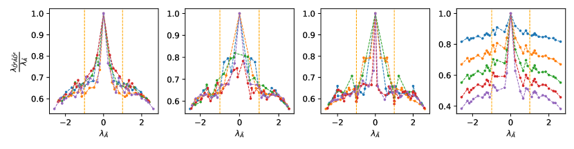
Figure 2: We use the metric $\frac{\lambda_{\tilde{D}^{\epsilon}\tilde{A}\tilde{D}^{\epsilon}}}{\lambda_{\tilde{A}}}$ to evaluate the shrinking effects of $\tilde{D}^{\epsilon}\tilde{A}\tilde{D}^{\epsilon}$ on the spectrum. We randomly sample 5 graphs in each of three datasets ZINC, MolPCBA and NCI1 respectively. In the first three figures, we use the fixed $\epsilon=-0.3$ on all 5 graphs. In the fourth figure, we use $\epsilon=-0.1,-0.2,-0.3,-0.4,-0.5$ respectively on one graph, which corresponds to the 5 lines from top to bottom. More visualization results on other datasets can be found in Appendix E.

To further investigate the effects of the normalization on the spectrum, we fix $\eta=0$ and empirically evaluate $\epsilon$ as shown in Fig. 2. When fixing $\epsilon$, $\tilde{D}^{\epsilon}\tilde{A}\tilde{D}^{\epsilon}$ shrinks the spectrum of $A$ with different degrees on different eigenvalues. For eigenvalues with small magnitudes (in the middle area of the spectrum), it has a small shrinking effect, while for eigenvalues with large magnitudes, it has a relatively large shrinking effect. Hence, $\tilde{D}^{\epsilon}\tilde{A}\tilde{D}^{\epsilon}$ can be used as a spectral smoothing method. Also, different $\epsilon$ results in different shrinking effects, which is consistent with the results in Proposition 4.1. Widely-used $\tilde{D}^{-\frac{1}{2}}\tilde{A}\tilde{D}^{-\frac{1}{2}}$ with the spectrum bounded by $[-1,1]$ may not be a good choice since the diminishing problem. Intuitively, to utilize more bases, we should narrow the range of the spectrum close to 1 (or -1) to avoid both the diminishing and divergence problems in higher-order bases. This can vary from different datasets and we should carefully balance $\epsilon$ and $k$.

5 Related Work

Many improvements on GNNs can be unified into the spectral smoothing operations, e.g. low-pass filter (Wu et al., 2019; Zhu et al., 2021; Klicpera et al., 2019a, b; Chien et al., 2021; Balcilar et al., 2021), alleviating oversmoothing (Ming Chen et al., 2020; Xu et al., 2018; Liu et al., 2020; Li et al., 2018), graph normalization(Cai et al., 2021), etc, our analysis on the relations of the correlation issue and the spectrum of underlying graph’s matrix provides a unified interpretation on their effectiveness.

ChebyNet (Defferrard et al., 2016), CayleNet (Levie et al., 2019), APPNP (Klicpera et al., 2019a), SSGC (Zhu & Koniusz, 2020), GPR (Chien et al., 2021), BernNet (He et al., 2021), etc explore various polynomial filters and use the normalized adjacency or Laplacian matrix as basis. We improve the approximation ability of polynomial filters by altering the spectrum of filter bases. The resulting bases allow leveraging more bases to approximate more sophisticated filters and are more suitable for learning coefficients from scratch.

We note that the concurrent work (Jin et al., 2022) has also pointed out the overcorrelation issue in the infinite depth case, without further discussion on the reason (e.g. graph’s spectrum) behind this phenomenon. In contrast, we show that correlation is inherently caused by the $unsmooth$ spectrum of the underlying graph filter, and also quantify this effect with spectral smoothness. It allows to analyze the correlation across all layers instead of only the theoretical infinite depth.

6 Experiments

We conduct experiments on TUDatasets (Yanardag & Vishwanathan, 2015; Kersting et al., 2016), OGB (Hu et al., 2020) which involve graph classification tasks and ZINC (Dwivedi et al., 2020) which involves graph regression tasks. Then, we evaluate the effects of our proposed new graph convolution architecture and two filter bases.

6.1 Results

Table 2: Results on TUDatasets. Higher is better.

dataset	NCI1	NCI109	ENZYMES	PTC_MR
GK	62.49$\pm$0.27	62.35$\pm$0.3	32.70$\pm$1.20	55.65$\pm$0.5
RW	-	-	24.16$\pm$1.64	55.91$\pm$0.3
PK	82.54$\pm$0.5	-	-	59.5$\pm$2.4
FGSD	79.80	78.84	-	62.8
AWE	-	-	35.77$\pm$5.93	-
DGCNN	74.44$\pm$0.47	-	51.0$\pm$7.29	58.59$\pm$2.5
PSCN	74.44$\pm$0.5	-	-	62.29$\pm$5.7
DCNN	56.61$\pm$1.04	-	-	-
ECC	76.82	75.03	45.67	-
DGK	80.31$\pm$0.46	80.32$\pm$0.3	53.43$\pm$0.91	60.08$\pm$2.6
GraphSag	76.0$\pm$1.8	-	58.2$\pm$6.0	-
CapsGNN	78.35$\pm$1.55	-	54.67$\pm$5.67	-
DiffPool	76.9$\pm$1.9	-	62.53	-
GIN	82.7$\pm$1.7	-	-	64.6$\pm$7.0
$k$-GNN	76.2	-	-	60.9
Spec-GN	84.79$\pm$1.63	83.62$\pm$0.75	72.50$\pm$5.79	68.05$\pm$6.41
Norm-GN	84.87$\pm$1.68	83.50$\pm$1.27	73.33$\pm$7.96	67.76$\pm$4.52

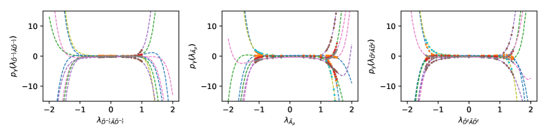
Figure 3: A visualization of the learned filters on ZINC. We tested on three bases with each basis randomly sampling 9 filters. Dots represent the eigenvalues of each basis. More visualization results on other datasets can be found in Appendix F.

Settings. We use the default dataset splits for OGB and ZINC. For TUDatasets, we follow the standard 10-fold cross-validation protocol and splits from (Zhang et al., 2018) and report our results following the protocol described in (Xu et al., 2019; Ying et al., 2018). Following all baselines on the leaderboard of ZINC, we control the number of parameters around 500K. The baseline models include: GK (Shervashidze et al., 2009), RW (Vishwanathan et al., 2010), PK (Neumann et al., 2016), FGSD (Verma & Zhang, 2017), AWE (Ivanov & Burnaev, 2018), DGCNN (Zhang et al., 2018), PSCN (Niepert et al., 2016), DCNN (Atwood & Towsley, 2016), ECC (Simonovsky & Komodakis, 2017), DGK (Yanardag & Vishwanathan, 2015), CapsGNN (Xinyi & Chen, 2019), DiffPool (Ying et al., 2018), GIN (Xu et al., 2019), $k$-GNN (Morris et al., 2019), GraphSage (Hamilton et al., 2017), GAT (Veličković et al., 2018), GatedGCN-PE (Bresson & Laurent, 2017), MPNN (sum) (Gilmer et al., 2017), DeeperG (Li et al., 2020), PNA (Corso et al., 2020), DGN (Beani et al., 2021), GSN (Bouritsas et al., 2020), GINE-VN (Brossard et al., 2020), GINE-APPNP (Brossard et al., 2020), PHC-GNN (Le et al., 2021), SAN (Kreuzer et al., 2021), Graphormer (Ying et al., 2021). Spec-GN denotes the proposed graph convolution in Eq. 9 with the smoothed filter basis by spectral transformation in Eq. 12. Norm-GN denotes the proposed graph convolution in Eq. 9 with the smoothed filter basis by graph normalization in Eq. 13.

Table 3: Results on ZINC (Lower is better) and MolPCBA (Higher is better).

method	ZINC MAE	MolPCBA AP
GCN	0.367$\pm$0.011 (505k)	24.24$\pm$0.34 (2.02m)
GIN	0.526$\pm$0.051 (510k)	27.03$\pm$0.23 (3.37m)
GAT	0.384$\pm$0.007 (531k)	-
GraphSage	0.398$\pm$0.002 (505k)	-
GatedGCN-PE	0.214$\pm$0.006 (505k)	-
MPNN	0.145$\pm$0.007 (481k)	-
DeeperG	-	28.42$\pm$0.43 (5.55m)
PNA	0.142$\pm$0.010 (387k)	28.38$\pm$0.35 (6.55m)
DGN	0.168$\pm$0.003 NA	28.85$\pm$0.30 (6.73m)
GSN	0.101$\pm$0.010 (523k)	-
GINE-VN	-	29.17$\pm$0.15 (6.15m)
GINE-APPNP	-	29.79$\pm$0.30 (6.15m)
PHC-GNN	-	29.47$\pm$0.26 (1.69m)
SAN	0.139$\pm$0.006 (509k)	-
Graphormer	0.122$\pm$0.006 (489k)	-
Spec-GN	0.0698$\pm$0.002 (503k)	29.65$\pm$0.28 (1.74m)
Norm-GN	0.0709$\pm$0.002 (500k)	29.51$\pm$0.33 (1.74m)

Results. Tab. 2 and 3 summarize performance of our approaches comparing with baselines on TUDatasets, ZINC and MolPCBA. For TUDatasets, we report the results of each model in its original paper by default. When the results are not given in the original paper, we report the best testing results given in (Zhang et al., 2018; Ivanov & Burnaev, 2018; Xinyi & Chen, 2019). For ZINC and MolPCBA, we report the results of their public leaderboards. TUDatasets involves small-scale datasets. NCI1 and NCI109 are around 4K graphs. ENZYMES and PTC_MR are under 1K graphs. General GNNs easily suffer from overfitting on these small-scale data, and therefore we can see that some traditional kernel-based methods even get better performance. However, Spec-GN and Norm-GN achieve higher classification accuracies by a large margin on these datasets. The results on TUDatasets show that although Spec-GN and Norm-GN achieve more expressive filters, it does not lead to overfitting on learning graph representations. Recently, Transformer-based models are quite popular in learning graph representations, and they significantly improve the results on large-scale molecular datasets. On ZINC, Spec-GN and Norm-GN outperform these Transformer-based models by a large margin. And on MolPCBA, they are also competitive compared with SOTA results.

Table 4: Ablation study results on ZINC with different settings.

Architecture		Basis				test MAE	valid MAE
shd	idp	$\tilde{D}^{-\frac{1}{2}}\tilde{A}\tilde{D}^{-\frac{1}{2}}$	$\tilde{D}^{-1}\tilde{A}$	$\tilde{A}_{\rho}$	$\tilde{D}^{\epsilon}\tilde{A}\tilde{D}^{\epsilon}$
✓		✓				0.1415$\pm$0.00748	0.1568$\pm$0.00729
✓			✓			0.1439$\pm$0.00900	0.1569$\pm$0.00739
✓				✓		0.1061$\pm$0.01018	0.1294$\pm$0.01454
✓					✓	0.1133$\pm$0.01711	0.1316$\pm$0.02057
	✓	✓				0.0944$\pm$0.00379	0.1100$\pm$0.00787
	✓		✓			0.0982$\pm$0.00417	0.1172$\pm$0.00666
	✓			✓		0.0698$\pm$0.00200	0.0884$\pm$0.00319
	✓				✓	0.0709$\pm$0.00176	0.0929$\pm$0.00445

6.2 Ablation Studies

We perform ablation studies on the proposed architecture and the filter bases $\tilde{A}_{\rho}$ (by setting $S=\tilde{A}$ in Eq. 12) and $\tilde{D}^{\epsilon}\tilde{A}\tilde{D}^{\epsilon}$ on ZINC. We use “idp” and “shd” to respectively represent the correlation-free architecture (also known as independent filter architecture) in Eq. 9 and the general shared filter architecture in Eq. 6. Both architectures learn the filter coefficients from scratch.

Correlation-free architecture and different filter bases. In Fig. 3, we visualize the learned filters in the correlation-free on three bases, i.e. $\tilde{D}^{-\frac{1}{2}}\tilde{A}\tilde{D}^{-\frac{1}{2}}$, $\tilde{A}_{\rho}$ and $\tilde{D}^{\epsilon}\tilde{A}\tilde{D}^{\epsilon}$. The visualizations show that each channel indeed learns a different filter on all three bases. $\tilde{D}^{-\frac{1}{2}}\tilde{A}\tilde{D}^{-\frac{1}{2}}$ has the bounded spectrum $[-1,1]$ that is slightly close to $1$ due to the involvement of self-loop. The filters learn a similar response on all range which corresponds to different frequencies in frequency domain. $\tilde{A}_{\rho}$ and $\tilde{D}^{\epsilon}\tilde{A}\tilde{D}^{\epsilon}$ have the spectrum close to $1$ or $-1$ while the filters learn diverse responses on these areas, which corresponds to more complex patterns on different frequencies. Tab. 4 shows that the correlation-free always outperforms the shared filter by a large margin on all tested bases. Both $\tilde{D}^{-\frac{1}{2}}\tilde{A}\tilde{D}^{-\frac{1}{2}}$ and $\tilde{D}^{-1}\tilde{A}$ have the bounded spectrum $[-1,1]$ and they have similar performance. $\tilde{A}_{\rho}$ and $\tilde{D}^{\epsilon}\tilde{A}\tilde{D}^{\epsilon}$ narrow the range of the spectrum close to $1$ or $-1$ through completely different strategies, but they have similar performance that is much better than $\tilde{D}^{-\frac{1}{2}}\tilde{A}\tilde{D}^{-\frac{1}{2}}$ and $\tilde{D}^{-1}\tilde{A}$. This validates our analysis on the filter basis. Meanwhile, $\tilde{A}_{\rho}$ achieves more accurate control on the spectrum, and correspondingly, it slightly outperforms $\tilde{D}^{\epsilon}\tilde{A}\tilde{D}^{\epsilon}$.

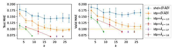
Figure 4: Ablation study results on ZINC with different number of bases $k$.

Do more bases gain improvements? In Fig. 4, we systematically evaluate the effects of the number of bases on learning graph representations, including $\tilde{D}^{-\frac{1}{2}}\tilde{A}\tilde{D}^{-\frac{1}{2}}$ and our $\tilde{A}_{\rho}$ with $\rho=1/3,1/6,1/7,1/8$. The shared filter case, i.e. shd$+\tilde{D}^{-\frac{1}{2}}\tilde{A}\tilde{D}^{-\frac{1}{2}}$ cannot well leverage more bases (a larger $k$) as the MAE stops decreasing at $0.150$ which is also reported by several baselines in Tab. 3. In contrast, both correlation-free cases idp$+\tilde{D}^{-\frac{1}{2}}\tilde{A}\tilde{D}^{-\frac{1}{2}}$ and idp$+\tilde{A}_{\rho}$ outperform the shared filter case by a large margin and they continuously gain improvements when increasing $k$. The MAE of idp$+\tilde{D}^{-\frac{1}{2}}\tilde{A}\tilde{D}^{-\frac{1}{2}}$ stops decreasing at the test MAE close to 0.09 and the valid MAE close to 0.11. By replacing $\tilde{D}^{-\frac{1}{2}}\tilde{A}\tilde{D}^{-\frac{1}{2}}$ with $\tilde{A}_{\rho}$, the best test MAE is below 0.07, and the best valid MAE is close to 0.088. The bases in $\tilde{A}_{\rho}$ are controlled by both $\rho$ and $k$. We use the tuple $(\rho,k)$ to denote a combination of $\rho$ and $k$. By fixing $\rho$, the curves corresponding to $\rho=1/3$ and $\rho=1/6$ show that increasing $k$ gains improvements. By fixing the upper bound of $\rho\times k$ to be 1, $(1/6,6)$ involves 3 more bases than $(1/3,3)$ and outperforms $(1/3,3)$. The same results are also reflected in the comparison of $(1/6,12)$ and $(1/3,6)$. For the comparison of $(1/6,18)$ and $(1/3,9)$, both settings achieve the lowest MAE and the difference is less obvious.

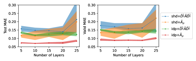
Figure 5: Ablation study results on ZINC with different number of layers.

The effects of model depth. Fig.5 shows the performance comparisons between correlation-free and shared filter as depth increases. Each architecture is tested with the default basis $\tilde{D}^{\frac{1}{2}}\tilde{A}\tilde{D}^{\frac{1}{2}}$ and our proposed $\tilde{A}_{\rho}$. We set the same number of bases in all resulting models, and each model is tested with the number of layers (depth) equal to $\{5,10,15,20,25\}$. The results show that the correlation-free can preserve the performance as depth increases. The shared filter cases perform quite unstable and drop dramatically when depth $>20$. Also, across all depths, the correlation-free almost always outperforms the shared filter and has low variance among different runs. In Appendix G, we also test cosine similarities of different layers in a deep model.

Stability. We also found that the correlation-free is more stable in different runs than the shared filter case as reflected in the standard deviation in Tab. 4. This is probably because different channels may pose different patterns, which causes interference among each other in the shared filter case. While the correlation-free well avoids this problem. Also, the results of $\tilde{A}_{\rho}$ and $\tilde{D}^{\epsilon}\tilde{A}\tilde{D}^{\epsilon}$ are more stable than $\tilde{D}^{-\frac{1}{2}}\tilde{A}\tilde{D}^{-\frac{1}{2}}$ and $\tilde{D}^{-1}\tilde{A}$ in different runs. For $\tilde{D}^{-\frac{1}{2}}\tilde{A}\tilde{D}^{-\frac{1}{2}}$ and $\tilde{D}^{-1}\tilde{A}$, the difference between the best and the worst runs can be more than 0.02. While for $\tilde{A}_{\rho}$ and $\tilde{D}^{\epsilon}\tilde{A}\tilde{D}^{\epsilon}$, this difference is less than 0.01. More results are given in Appendix H. The instability of $\tilde{D}^{-\frac{1}{2}}\tilde{A}\tilde{D}^{-\frac{1}{2}}$ and $\tilde{D}^{-1}\tilde{A}$ is probably because learning filter coefficients from scratch without any constraints is difficult to maintain spectrum properties and therefore easily falls into an ill-posed filter (He et al., 2021). In contrast, $\tilde{A}_{\rho}$ and $\tilde{D}^{\epsilon}\tilde{A}\tilde{D}^{\epsilon}$ inherently with smoother spectrum alleviate this problem and make them more appropriate in the scenario of learning coefficients from scratch.

7 Conclusion

We study the effects of spectrum in GNNs. It shows that in existing architectures, the unsmooth spectrum results in the correlation issue, which acts as the obstacle to developing deep models as well as applying more powerful graph filters. Based on this observation, we propose the correlation-free architecture which decouples the correlation issue from filter design. Then, we show that the spectral characteristics also hinder the approximation abilities of polynomial filters and address it by altering the graph’s spectrum. Our extensive experiments show the significant performance gain of correlation-free architecture with powerful filters.

Appendix A Derivations of Eq. 7 and Eq. 8

Since $\mathcal{S}\in\mathbb{R}^{n\times n}$ is a symmetric matrix, assume the eigendecomposition $\mathcal{S}=P\Lambda P^{\top}$ with $P=\bigl{(}\bm{p}_{1},\bm{p}_{2},\dots,\bm{p}_{n}\bigr{)}$ and $\|\bm{p}_{i}\|=1,i\in[n]$.

$$\cos\bigl{(}\langle\bm{h},\bm{p}_{i}\rangle\bigr{)} =\frac{\bm{h}^{\top}\bm{p}_{i}}{\|\bm{h}\|\|\bm{p}_{i}\|}$$

$$=\frac{\bm{h}^{\top}\bm{p}_{i}}{\|\bm{h}\|}$$

$$=\frac{\bm{h}^{\top}\bm{p}_{i}}{\sqrt{\bm{h}^{\top}\bm{h}}}$$

$$=\frac{\bm{h}^{\top}\bm{p}_{i}}{\sqrt{(P^{\top}\bm{h})^{\top}P^{\top}\bm{h}}}$$

$$=\frac{\bm{h}^{\top}\bm{p}_{i}}{\sqrt{\sum^{n}_{j=1}\bigl{(}\bm{p}_{j}^{\top}\bm{h}\bigr{)}^{2}}}$$

$$=\frac{\bm{h}^{\top}\bm{p}_{i}}{\sqrt{\sum^{n}_{j=1}\bigl{(}\bm{h}^{\top}\bm{p}_{j}\bigr{)}^{2}}}$$

$$=\frac{\alpha_{i}}{\sqrt{\sum^{n}_{j=1}\alpha_{j}^{2}}}.$$

$$\cos\bigl{(}\langle\mathcal{S}\bm{h},\bm{p}_{i}\rangle\bigr{)} =\frac{\bigl{(}\mathcal{S}\bm{h}\bigr{)}^{\top}\bm{p}_{i}}{\|\mathcal{S}\bm{h}\|\|\bm{p}_{i}\|}$$

$$=\frac{\bigl{(}\mathcal{S}\bm{h}\bigr{)}^{\top}\bm{p}_{i}}{\sqrt{\bigl{(}\mathcal{S}\bm{h}\bigr{)}^{\top}\mathcal{S}\bm{h}}}$$

$$=\frac{\bigl{(}P\Lambda\bigl{(}P^{\top}\bm{h}\bigr{)}\bigr{)}^{\top}\bm{p}_{i}}{\sqrt{\bigl{(}P\Lambda\bigl{(}P^{\top}\bm{h}\bigr{)}\bigr{)}^{\top}\bigl{(}P\Lambda\bigl{(}P^{\top}\bm{h}\bigr{)}\bigr{)}}}$$

$$=\frac{\bigl{(}P^{\top}\bm{h}\bigr{)}^{\top}\Lambda P^{\top}\bm{p}_{i}}{\sqrt{\bigl{(}P^{\top}\bm{h}\bigr{)}^{\top}\Lambda^{2}\bigl{(}P^{\top}\bm{h}\bigr{)}}}$$

$$=\frac{\begin{pmatrix}\bm{p}_{1}^{\top}\bm{h},\dots,\bm{p}_{i}^{\top}\bm{h},\dots,\bm{p}_{n}^{\top}\bm{h}\end{pmatrix}\begin{pmatrix}\lambda_{1}\\ &\ddots\\ &&\lambda_{i}\\ &&&\ddots\\ &&&&\lambda_{n}\\ \end{pmatrix}\begin{pmatrix}\bm{p}_{1}^{\top}\\ \vdots\\ \bm{p}_{i}^{\top}\\ \vdots\\ \bm{p}_{n}^{\top}\\ \end{pmatrix}\begin{pmatrix}\bm{p}_{i}\end{pmatrix}}{\sqrt{\bigl{(}P^{\top}\bm{h}\bigr{)}^{\top}\Lambda^{2}\bigl{(}P^{\top}\bm{h}\bigr{)}}}$$

$$=\frac{\bm{p}_{i}^{\top}\bm{h}\lambda_{i}}{\sqrt{\sum^{n}_{j=1}\bigl{(}\bm{p}_{j}^{\top}\bm{h}\bigr{)}^{2}\lambda_{j}^{2}}}$$

$$=\frac{\bm{h}^{\top}\bm{p}_{i}\lambda_{i}}{\sqrt{\sum^{n}_{j=1}\bigl{(}\bm{h}^{\top}\bm{p}_{j}\bigr{)}^{2}\lambda_{j}^{2}}}$$

$$=\frac{\alpha_{i}\lambda_{i}}{\sqrt{\sum^{n}_{j=1}\alpha_{j}^{2}\lambda_{j}^{2}}}$$

Appendix B Proof of Proposition 3.1

Proof.

(i) As $\mathcal{S}^{k}=P\Lambda^{k}P^{\top}$ and Eq. 8, for $k=0,1,2,\dots,+\infty$, we have

$$|\cos(\langle\mathcal{S}^{k}\bm{h},\bm{p}_{1}\rangle)| =\frac{|\alpha_{1}\lambda_{1}^{k}|}{\sqrt{\sum^{n}_{i=1}\alpha_{i}^{2}\lambda_{i}^{2k}}}$$

$$=\frac{|\lambda_{1}|}{|\lambda_{1}|}\frac{|\alpha_{1}\lambda_{1}^{k}|}{\sqrt{\sum^{n}_{i=1}\alpha_{i}^{2}\lambda_{i}^{2k}}}$$

$$=\frac{|\alpha_{1}\lambda_{1}^{k+1}|}{\sqrt{\lambda_{1}^{2}\sum^{n}_{i=1}\alpha_{i}^{2}\lambda_{i}^{2k}}}$$

$$\leq\frac{|\alpha_{1}\lambda_{1}^{k+1}|}{\sqrt{\sum^{n}_{i=1}\alpha_{i}^{2}\lambda_{i}^{2(k+1)}}}$$

$$=|\cos(\langle\mathcal{S}^{k+1}\bm{h},\bm{p}_{1}\rangle)|.$$

Similarly, we can prove that $|\cos(\langle\mathcal{S}^{k}\bm{h},\bm{p}_{n}\rangle)|\geq|\cos(\langle\mathcal{S}^{k+1}\bm{h},\bm{p}_{n}\rangle)|$.

(ii) Since $|\cos(\langle\mathcal{S}^{k}\bm{h},\bm{p}_{n}\rangle)|$ monotonously increases with respect to $k$ and has the upper bound 1, $|\cos(\langle\mathcal{S}^{k}\bm{h},\bm{p}_{n}\rangle)|$ must be convergent.

$$\lim\limits_{k\rightarrow\infty}|\cos(\langle\mathcal{S}^{k}\bm{h},\bm{p}_{1}\rangle)| =\lim\limits_{k\rightarrow\infty}\frac{|\alpha_{1}\lambda_{1}^{k}|}{\sqrt{\sum^{n}_{i=1}\alpha_{i}^{2}\lambda_{i}^{2k}}}$$

$$=\lim\limits_{k\rightarrow\infty}\frac{|\alpha_{1}|}{\sqrt{\alpha_{1}^{2}+\sum^{n}_{i=2}\alpha_{i}^{2}\bigl{(}\frac{\lambda_{i}}{\lambda_{1}}\bigr{)}^{2k}}}$$

$$=\frac{|\alpha_{1}|}{\sqrt{\alpha_{1}^{2}+\lim\limits_{k\rightarrow\infty}\sum^{n}_{i=2}\alpha_{i}^{2}\bigl{(}\frac{\lambda_{i}}{\lambda_{1}}\bigr{)}^{2k}}}$$

As $|\lambda_{1}|>|\lambda_{2}|\geq,\dots,\geq|\lambda_{n}|$, we have $\lim\limits_{k\rightarrow\infty}\sum^{n}_{i=2}\alpha_{i}^{2}\bigl{(}\frac{\lambda_{i}}{\lambda_{1}}\bigr{)}^{2k}=0$ and the convergence speed is decided by $|\frac{\lambda_{2}}{\lambda_{1}}|$. Therefore $\lim\limits_{k\rightarrow\infty}|\cos(\langle\mathcal{S}^{k}\bm{h},\bm{p}_{1}\rangle)|=1$.

$$\cos\bigl{(}\langle\mathcal{S}\bm{h},\mathcal{S}\bm{h}^{\prime}\rangle\bigr{)} =\frac{\bigl{(}\mathcal{S}\bm{h}\bigr{)}^{\top}\mathcal{S}\bm{h}^{\prime}}{\|\mathcal{S}\bm{h}\|\|\mathcal{S}\bm{h}^{\prime}\|}$$

$$=\frac{\bigl{(}\mathcal{S}\bm{h}\bigr{)}^{\top}\mathcal{S}\bm{h}^{\prime}}{\sqrt{\bigl{(}\mathcal{S}\bm{h}\bigr{)}^{\top}\mathcal{S}\bm{h}}\sqrt{\bigl{(}\mathcal{S}\bm{h}^{\prime}\bigr{)}^{\top}\mathcal{S}\bm{h}^{\prime}}}$$

$$=\frac{\bigl{(}P\Lambda\bigl{(}P^{\top}\bm{h}\bigr{)}\bigr{)}^{\top}P\Lambda\bigl{(}P^{\top}\bm{h}^{\prime}\bigr{)}}{\sqrt{\bigl{(}P\Lambda\bigl{(}P^{\top}\bm{h}\bigr{)}\bigr{)}^{\top}\bigl{(}P\Lambda\bigl{(}P^{\top}\bm{h}\bigr{)}\bigr{)}}\sqrt{\bigl{(}P\Lambda\bigl{(}P^{\top}\bm{h}^{\prime}\bigr{)}\bigr{)}^{\top}\bigl{(}P\Lambda\bigl{(}P^{\top}\bm{h}^{\prime}\bigr{)}\bigr{)}}}$$

$$=\frac{\bigl{(}P^{\top}\bm{h}\bigr{)}^{\top}\Lambda^{2}P^{\top}\bm{h}^{\prime}}{\sqrt{\bigl{(}P^{\top}\bm{h}\bigr{)}^{\top}\Lambda^{2}\bigl{(}P^{\top}\bm{h}\bigr{)}}\sqrt{\bigl{(}P^{\top}\bm{h}^{\prime}\bigr{)}^{\top}\Lambda^{2}\bigl{(}P^{\top}\bm{h}^{\prime}\bigr{)}}}$$

$$=\frac{\bm{\alpha}^{\top}\Lambda^{2}\bm{\beta}}{\sqrt{\bm{\alpha}^{\top}\Lambda^{2}\bm{\alpha}}\sqrt{\bm{\beta}^{\top}\Lambda^{2}\bm{\beta}}}$$

$$=\frac{\sum^{n}_{i=1}\alpha_{i}\beta_{i}\lambda_{i}^{2}}{\sqrt{\sum^{n}_{i=1}\alpha_{i}^{2}\lambda_{i}^{2}}\sqrt{\sum^{n}_{i=1}\beta_{i}^{2}\lambda_{i}^{2}}}$$

Then,

$$\lim\limits_{k\rightarrow\infty}|\cos(\langle\mathcal{S}^{k}\bm{h},\mathcal{S}^{k}\bm{h}^{\prime}\rangle)| =\lim\limits_{k\rightarrow\infty}\frac{\bigl{|}\sum^{n}_{i=1}\alpha_{i}\beta_{i}\lambda_{i}^{2k}\bigr{|}}{\sqrt{\sum^{n}_{i=1}\alpha_{i}^{2}\lambda_{i}^{2k}}\sqrt{\sum^{n}_{i=1}\beta_{i}^{2}\lambda_{i}^{2k}}}$$

$$=\lim\limits_{k\rightarrow\infty}\frac{\bigl{|}\sum^{n}_{i=1}\alpha_{i}\beta_{i}\frac{\lambda_{i}}{\lambda_{1}}^{2k}\bigr{|}}{\sqrt{\sum^{n}_{i=1}\alpha_{i}^{2}\frac{\lambda_{i}}{\lambda_{1}}^{2k}}\sqrt{\sum^{n}_{i=1}\beta_{i}^{2}\frac{\lambda_{i}}{\lambda_{1}}^{2k}}}$$

$$=\lim\limits_{k\rightarrow\infty}\frac{\bigl{|}\alpha_{1}\beta_{1}+\sum^{n}_{i=2}\alpha_{i}\beta_{i}\frac{\lambda_{i}}{\lambda_{1}}^{2k}\bigr{|}}{\sqrt{\alpha_{1}^{2}+\sum^{n}_{i=2}\alpha_{i}^{2}\frac{\lambda_{i}}{\lambda_{1}}^{2k}}\sqrt{\beta_{1}^{2}+\sum^{n}_{i=2}\beta_{i}^{2}\frac{\lambda_{i}}{\lambda_{1}}^{2k}}}$$

$$=\frac{\bigl{|}\alpha_{1}\beta_{1}\bigr{|}}{\sqrt{\alpha_{1}^{2}}\sqrt{\beta_{1}^{2}}}$$

$$=1$$

∎

Appendix C More Discussions of Spectral Optimization on Filter Basis

We use $\textrm{E}_{(S,\lambda)}$ to denote the eigenspace of $S$ associated with $\lambda$ such that $\textrm{E}_{(S,\lambda)}=\{\bm{v}:(S-\lambda I)\bm{v}=\bm{0}\}$.

Proposition C.1.

Given a symmetric matrix $S\in\mathbb{R}^{n\times n}$ with $S=P\Lambda P^{\top}$ where $\Lambda=\textrm{diag}(\lambda_{1},\lambda_{2},\dots,\lambda_{n})$, and $P$ can be any eigenbasis of $S$, let $S_{\phi}=P\phi(\Lambda)P^{\top}$, where $\phi(\cdot)$ is an entry-wise function applied on $\Lambda$. Then we have
(i) $\textrm{E}_{(S,\lambda_{i})}\subseteq\textrm{E}_{(S_{\phi},\phi(\lambda_{i}))},i\in[n]$;
(ii) Meanwhile, if $\phi(\cdot)$ is injective, $\textrm{E}_{(S,\lambda_{i})}=\textrm{E}_{(S_{\phi},\phi(\lambda_{i}))}$ and $\mathcal{F}_{\phi}(S)=P\phi(\Lambda)P^{\top}$ is injective.

Proof.

Let $P=(\bm{p}_{1},\bm{p}_{2},\dots,\bm{p}_{n})$. $S=P\Lambda P^{\top}$ is equivalent to $S\bm{p}_{i}=\lambda_{i}\bm{p}_{i},i\in[n]$. For any $i\in[n]$, the geometric multiplicity of any $\lambda_{i}$ is equal to its algebraic multiplicity, and $\textrm{E}_{(S,\lambda_{i})}=\textrm{Span}(\{\bm{p}_{k}|\lambda_{k}=\lambda_{i},k\in[n]\})$. $S_{\phi}=P\phi(\Lambda)P^{\top}$ and $S_{\phi}\bm{p}_{i}=\phi(\lambda_{i})\bm{p}_{i},i\in[n]$. Similarly, for any $i\in[n]$, $\textrm{E}_{(S_{\phi},\phi(\lambda_{i}))}=\textrm{Span}(\{\bm{p}_{k}|\phi(\lambda_{k})=\phi(\lambda_{i}),k\in[n]\})$. Note that $\{\bm{p}_{k}|\lambda_{k}=\lambda_{i},k\in[n]\}\subseteq\{\bm{p}_{k}|\phi(\lambda_{k})=\phi(\lambda_{i}),k\in[n]\}$ for any $i\in[n]$. Hence $\textrm{Span}(\{\bm{p}_{k}|\lambda_{k}=\lambda_{i},k\in[n]\})\subseteq\textrm{Span}(\{\bm{p}_{k}|\phi(\lambda_{k})=\phi(\lambda_{i}),k\in[n]\}$. As a result, $\textrm{E}_{(S,\lambda_{i})}\subseteq\textrm{E}_{(S_{\phi},\phi(\lambda_{i}))}$ for any $i\in[n])$.

If $\phi(\cdot)$ is injective, $\{\bm{p}_{k}|\lambda_{k}=\lambda_{i},k\in[n]\}=\{\bm{p}_{k}|\phi(\lambda_{k})=\phi(\lambda_{i}),k\in[n]\}$ for any $i\in[n]$. Thus $\textrm{E}_{(S,\lambda_{i})}=\textrm{E}_{(S_{\phi},\phi(\lambda_{i}))}$.

We use $\sigma(S)$ to denote the generalisation of the set of all eigenvalues of $S$ (Slso known as the spectrum of $S$). Let $S=P\Lambda_{1}P^{\top}$ and $B=Q\Lambda_{2}Q^{\top}$. Suppose $S\neq B$, to prove $S_{\phi}=\mathcal{F}_{\phi}(S)\neq B_{\phi}=\mathcal{F}_{\phi}(B)$, we discuss two cases respectively.

Case 1: $\sigma(S)\neq\sigma(B)$

Then $\sigma(S_{\phi})\neq\sigma(B_{\phi})$. The characteristic polynomials of $S_{\phi}$ and $B_{\phi}$ are different. Therefore, $S_{\phi}\neq B_{\phi}$.

Case 2: $\sigma(S)=\sigma(B)$

Then $\Lambda_{1}=\Lambda_{2}=\Lambda$. We prove the equivalent proposition ”$S_{\phi}=B_{\phi}\Rightarrow S=B$”. If $S_{\phi}=B_{\phi}$, $P\phi(\Lambda)P^{\top}=Q\phi(\Lambda)Q^{\top}$. For any $\lambda_{i}$ with geometric multiplicity $k$, we can find the corresponding eigenvectors $\bm{p}_{1},\bm{p}_{2},\dots,\bm{p}_{k}$ according to $P\phi(\Lambda)P^{\top}$. Similarly, we can find the corresponding eigenvectors $\bm{q}_{1},\bm{q}_{2},\dots,\bm{q}_{k}$ according to $Q\phi(\Lambda)Q^{\top}$. Note that the eigen-decomposition is unique in terms of eigenspaces. Thus, $\textrm{E}_{(S_{\phi},\phi(\lambda_{i}))}=\textrm{Span}(\bm{p}_{1},\bm{p}_{2},\dots,\bm{p}_{k})=\textrm{Span}(\bm{q}_{1},\bm{q}_{2},\dots,\bm{q}_{k})=\textrm{E}_{(B_{\phi},\phi(\lambda_{i}))}$. Therefore, for any $\lambda_{i}$, $\textrm{E}_{(S,\lambda_{i})}=\textrm{E}_{(B,\lambda_{i})}$ (As given in Proposition C.1). Correspondingly, $S=P\Lambda P^{\top}=Q\Lambda Q^{\top}=B$.

∎

Proposition C.1 shows that the eigenspace of $S_{\phi}$ involves the eigenspace of $S$. Therefore, $S_{\phi}$ is invariant to the choice of eigenbasis, i.e., $S_{\phi}=P\phi(\Lambda)P^{\top}=P^{\prime}\phi(\Lambda)P^{\prime\top}$ for any eigenbases $P$ and $P^{\prime}$ of $S$. Hence, $S_{\phi}$ is unique to $S$ for a given $\phi(\cdot)$. Consistently, we denote the mapping $\mathcal{F}_{\phi}(S)=\mathcal{F}_{\phi}(P\Lambda P^{\top})=P\phi(\Lambda)P^{\top}$.

When $\mathcal{F}_{\phi}$ is injective, $\mathcal{F}_{\phi}(S)$ and $S$ share the same algebraic multiplicity. Otherwise, $\mathcal{F}_{\phi}(S)$ has a larger algebraic multiplicity on the corresponding eigenvalues, which may weaken the approximation ability based on the understanding of Vandermonde matrix. Also, the injectivity of $\mathcal{F}_{\phi}$ serves as a guarantee that the transformation is reversible with no information loss.

$\mathcal{F}_{\phi}(\cdot)$ is also equivariant to graph isomorphism. For any two graphs $G_{1}$ and $G_{2}$ with matrix representations $S_{1}$ and $S_{2}$ (e.g., adjacency matrix, Laplacian matrix, etc.), $G_{1}$ and $G_{2}$ are isomorphic if and only if there exists a permutation matrix $M$ such that $MS_{1}M^{\top}=S_{2}$. We denote $I(S)=MSM^{\top}$. Then

Claim 1.

$\mathcal{F}_{\phi}(\cdot)$ is equivariant to graph isomorphism, i.e. $\mathcal{F}_{\phi}(I(S))=I(\mathcal{F}_{\phi}(S))$.

Proof.

$$\mathcal{F}_{\phi}(I(S)) =\mathcal{F}_{\phi}(MSM^{\top})$$

$$=\mathcal{F}_{\phi}(M(P\Lambda P^{\top})M^{\top})$$

$$=\mathcal{F}_{\phi}((MP)\Lambda(MP)^{\top})$$

$$=(MP)\phi(\Lambda)(MP)^{\top}$$

$$=M(P\phi(\Lambda)P^{\top})M^{\top}$$

$$=I(\mathcal{F}_{\phi}(S))$$

∎

Hence, for a specific GNN model $f_{\textrm{GNN}}$, $f_{\textrm{GNN}}(\mathcal{F}_{\phi}(I(S)))=f_{\textrm{GNN}}(I(\mathcal{F}_{\phi}(S)))=f_{\textrm{GNN}}(\mathcal{F}_{\phi}(S))$. The learned representation is invariant to graph isomorphism (also known as permutation invariance (Zaheer et al., 2017; Murphy et al., 2019)) when introducing $\mathcal{F}_{\phi}(\cdot)$.

Appendix D Proof of Proposition 4.1

Proof.

Let $\mathring{A}=(D+\eta I)^{\epsilon}(A+\eta I)(D+\eta I)^{\epsilon}$. According to Courant-Fischer theorem,

$$\mu_{i}=\min_{\mathrm{dim}(S)=i}\max_{x\in S}\frac{\bm{x}^{\top}\mathring{A}\bm{x}}{\bm{x}^{\top}\bm{x}}.$$

Let $\bm{y}=(D+\eta I)^{\epsilon}\bm{x}$. As the change of variables $\bm{y}=(D+\eta I)^{\epsilon}\bm{x}$ is non-singular, this is equivalent to

$$\mu_{i}=\min_{\mathrm{dim}(T)=i}\max_{\bm{y}\in T}\frac{\bm{y}^{\top}(A+\eta I)\bm{y}}{\bm{y}^{\top}(D+\eta I)^{-2\epsilon}\bm{y}}.$$

Therefore,

$$\mu_{i} =\min_{\mathrm{dim}(T)=i}\max_{\bm{y}\in T}\frac{\bm{y}^{\top}(A+\eta I)\bm{y}}{\bm{y}^{\top}(D+\eta I)^{-2\epsilon}\bm{y}}$$

$$\geq\min_{\mathrm{dim}(T)=i}\max_{\bm{y}\in T}\frac{\bm{y}^{\top}(A+\eta I)\bm{y}}{(d_{\mathrm{max}}+\eta)^{-2\epsilon}\bm{y}^{\top}\bm{y}}$$

$$=(d_{\mathrm{max}}+\eta)^{2\epsilon}\bigl{(}\min_{\mathrm{dim}(T)=i}\max_{\bm{y}\in T}\frac{\bm{y}^{\top}A\bm{y}}{\bm{y}^{\top}\bm{y}}+\eta\bigr{)}$$

$$=(\lambda_{i}+\eta)(d_{\mathrm{max}}+\eta)^{2\epsilon}.$$

Similarly, we can prove $\mu_{i}\leq(\lambda_{i}+\eta)(d_{\mathrm{min}}+\eta)^{2\epsilon}$. ∎

Appendix E Visualizations of the Effects of the Normalization $\tilde{D}^{\epsilon}\tilde{A}\tilde{D}^{\epsilon}$ on the Spectrum

Figure 6: We randomly sample 5 graphs in each of three datasets NCI109, ENZYMES and PTC_MR respectively. And we use the fixed $\epsilon=-0.3$ to see the effects of the normalization on all graphs.

Appendix F Visualizations of the Learned Filters

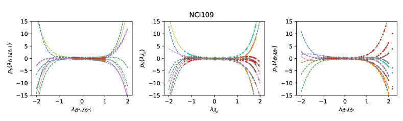
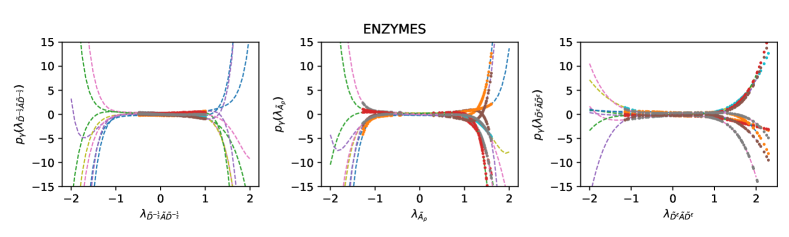
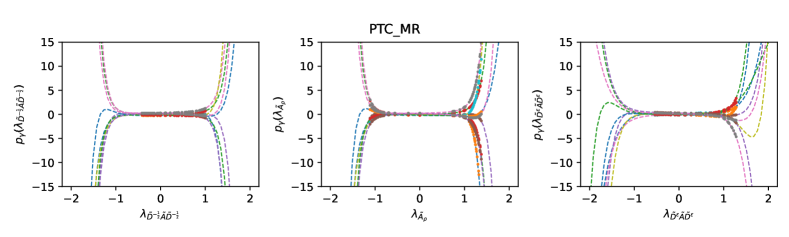
Figure 7: Visualizations of the learned filters on MolPCBA, NCI1, NCI109, ENZYMES and PTC_MR.

Appendix G The Correlation Issue of Deep Models

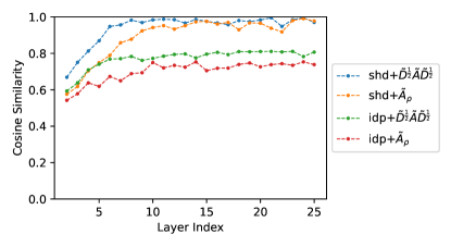
Figure 8: Cosine similarities on ZINC.

We test the absolute value of cosine similarities in different layers for a depth=25 model. For each graph, we compute the mean of all hidden signal pairs. The final visualized results in Fig.8 are the mean of all graphs within a randomly selected batch. To be consistent with the definition of spectral graph convolution as well as our correlation analysis, the test runs do not utilize edge features of ZINC.

The results show that on both bases, the cosine of the shared filter case converges to 1, while the correlation-free converges to $0.8$ for $\tilde{D}^{\frac{1}{2}}\tilde{A}\tilde{D}^{\frac{1}{2}}$ and $0.7$ for $\tilde{A}_{\rho}$. (We also found that it easily leads to a large cosine similarity on ZINC, which is mainly because graphs are small such that $n<<d$, where $n$ is the number of nodes and $d$ is the number of hidden features.) These results do show that general GNNs suffer from the correlation issue as depth increases, while our correlation-free architecture enjoys a relatively stable performance.

Appendix H More Results

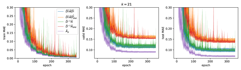
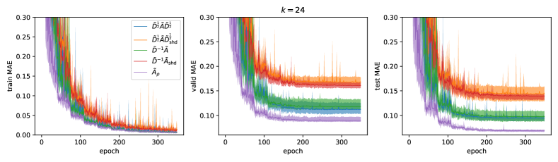
Figure 9: The curves of 5 runs on ZINC with the number of basis $k=9,18,21,24$.

References

- Atwood & Towsley (2016) Atwood, J. and Towsley, D. Diffusion-convolutional neural networks. In Advances in Neural Information Processing Systems, pp. 1993–2001, 2016.
- Balcilar et al. (2021) Balcilar, M., Renton, G., Héroux, P., Gaüzère, B., Adam, S., and Honeine, P. Analyzing the expressive power of graph neural networks in a spectral perspective. In International Conference on Learning Representations, 2021. URL https://openreview.net/forum?id=-qh0M9XWxnv.
- Beani et al. (2021) Beani, D., Passaro, S., Létourneau, V., Hamilton, W., Corso, G., and Liò, P. Directional graph networks. In International Conference on Machine Learning, pp. 748–758. PMLR, 2021.
- Bo et al. (2021) Bo, D., Wang, X., Shi, C., and Shen, H. Beyond low-frequency information in graph convolutional networks. In AAAI. AAAI Press, 2021.
- Bouritsas et al. (2020) Bouritsas, G., Frasca, F., Zafeiriou, S., and Bronstein, M. M. Improving graph neural network expressivity via subgraph isomorphism counting. arXiv preprint arXiv:2006.09252, 2020.
- Bresson & Laurent (2017) Bresson, X. and Laurent, T. Residual gated graph convnets. arXiv preprint arXiv:1711.07553, 2017.
- Brossard et al. (2020) Brossard, R., Frigo, O., and Dehaene, D. Graph convolutions that can finally model local structure. arXiv preprint arXiv:2011.15069, 2020.
- Cai et al. (2021) Cai, T., Luo, S., Xu, K., He, D., Liu, T.-Y., and Wang, L. Graphnorm: A principled approach to accelerating graph neural network training. In 2021 International Conference on Machine Learning, May 2021.
- Chien et al. (2021) Chien, E., Peng, J., Li, P., and Milenkovic, O. Adaptive universal generalized pagerank graph neural network. In International Conference on Learning Representations, 2021. URL https://openreview.net/forum?id=n6jl7fLxrP.
- Corso et al. (2020) Corso, G., Cavalleri, L., Beaini, D., Liò, P., and Veličković, P. Principal neighbourhood aggregation for graph nets. In Advances in Neural Information Processing Systems, 2020.
- Defferrard et al. (2016) Defferrard, M., Bresson, X., and Vandergheynst, P. Convolutional neural networks on graphs with fast localized spectral filtering. In Advances in neural information processing systems, pp. 3844–3852, 2016.
- Dwivedi et al. (2020) Dwivedi, V. P., Joshi, C. K., Laurent, T., Bengio, Y., and Bresson, X. Benchmarking graph neural networks. arXiv preprint arXiv:2003.00982, 2020.
- Gao et al. (2021) Gao, X., Dai, W., Li, C., Zou, J., Xiong, H., and Frossard, P. Message passing in graph convolution networks via adaptive filter banks. arXiv preprint arXiv:2106.09910, 2021.
- Gilmer et al. (2017) Gilmer, J., Schoenholz, S. S., Riley, P. F., Vinyals, O., and Dahl, G. E. Neural message passing for quantum chemistry. In Proceedings of the 34th International Conference on Machine Learning-Volume 70, pp. 1263–1272. JMLR. org, 2017.
- Hamilton et al. (2017) Hamilton, W., Ying, Z., and Leskovec, J. Inductive representation learning on large graphs. In Advances in Neural Information Processing Systems, pp. 1024–1034, 2017.
- Hammond et al. (2011) Hammond, D. K., Vandergheynst, P., and Gribonval, R. Wavelets on graphs via spectral graph theory. Applied and Computational Harmonic Analysis, 30(2):129–150, 2011.
- He et al. (2021) He, M., Wei, Z., Huang, Z., and Xu, H. Bernnet: Learning arbitrary graph spectral filters via bernstein approximation. In NeurIPS, 2021.
- Hu et al. (2020) Hu, W., Fey, M., Zitnik, M., Dong, Y., Ren, H., Liu, B., Catasta, M., and Leskovec, J. Open graph benchmark: Datasets for machine learning on graphs. arXiv preprint arXiv:2005.00687, 2020.
- Huang et al. (2020) Huang, W., Rong, Y., Xu, T., Sun, F., and Huang, J. Tackling over-smoothing for general graph convolutional networks. arXiv preprint arXiv:2008.09864, 2020.
- Ivanov & Burnaev (2018) Ivanov, S. and Burnaev, E. Anonymous walk embeddings. In Dy, J. and Krause, A. (eds.), Proceedings of the 35th International Conference on Machine Learning, volume 80 of Proceedings of Machine Learning Research, pp. 2191–2200, Stockholmsmässan, Stockholm Sweden, 10–15 Jul 2018. PMLR. URL http://proceedings.mlr.press/v80/ivanov18a.html.
- Jin et al. (2022) Jin, W., Liu, X., Ma, Y., Aggarwal, C., and Tang, J. Towards feature overcorrelation in deeper graph neural networks, 2022. URL https://openreview.net/forum?id=Mi9xQBeZxY5.
- Kersting et al. (2016) Kersting, K., Kriege, N. M., Morris, C., Mutzel, P., and Neumann, M. Benchmark data sets for graph kernels, 2016. http://graphkernels.cs.tu-dortmund.de.
- Kipf & Welling (2017) Kipf, T. N. and Welling, M. Semi-supervised classification with graph convolutional networks. In International Conference on Learning Representations (ICLR), 2017.
- Klicpera et al. (2019a) Klicpera, J., Bojchevski, A., and Günnemann, S. Predict then propagate: Graph neural networks meet personalized pagerank. In International Conference on Learning Representations (ICLR), 2019a.
- Klicpera et al. (2019b) Klicpera, J., Weißenberger, S., and Günnemann, S. Diffusion improves graph learning. Advances in Neural Information Processing Systems, 32:13354–13366, 2019b.
- Kreuzer et al. (2021) Kreuzer, D., Beaini, D., Hamilton, W., Létourneau, V., and Tossou, P. Rethinking graph transformers with spectral attention. arXiv preprint arXiv:2106.03893, 2021.
- Le et al. (2021) Le, T., Bertolini, M., Noé, F., and Clevert, D.-A. Parameterized hypercomplex graph neural networks for graph classification. arXiv preprint arXiv:2103.16584, 2021.
- Levie et al. (2019) Levie, R., Monti, F., Bresson, X., and Bronstein, M. M. Cayleynets: Graph convolutional neural networks with complex rational spectral filters. IEEE Transactions on Signal Processing, 67(1):97–109, 2019. doi: 10.1109/TSP.2018.2879624.
- Li et al. (2020) Li, G., Xiong, C., Thabet, A., and Ghanem, B. Deepergcn: All you need to train deeper gcns. arXiv preprint arXiv:2006.07739, 2020.
- Li et al. (2018) Li, Q., Han, Z., and Wu, X.-M. Deeper insights into graph convolutional networks for semi-supervised learning. In Thirty-Second AAAI Conference on Artificial Intelligence, 2018.
- Liu et al. (2020) Liu, M., Gao, H., and Ji, S. Towards deeper graph neural networks. In Proceedings of the 26th ACM SIGKDD International Conference on Knowledge Discovery & Data Mining, pp. 338–348, 2020.
- Ming Chen et al. (2020) Ming Chen, Z. W., Zengfeng Huang, B. D., and Li, Y. Simple and deep graph convolutional networks. 2020.
- Morris et al. (2019) Morris, C., Ritzert, M., Fey, M., Hamilton, W. L., Lenssen, J. E., Rattan, G., and Grohe, M. Weisfeiler and leman go neural: Higher-order graph neural networks. In Proceedings of the AAAI Conference on Artificial Intelligence, volume 33, pp. 4602–4609, 2019.
- Muhammet et al. (2020) Muhammet, B., Guillaume, R., Pierre, H., Benoit, G., Sébastien, A., and Honeine, P. When spectral domain meets spatial domain in graph neural networks. In Thirty-seventh International Conference on Machine Learning (ICML 2020)-Workshop on Graph Representation Learning and Beyond (GRL+ 2020), 2020.
- Murphy et al. (2019) Murphy, R. L., Srinivasan, B., Rao, V., and Ribeiro, B. Janossy pooling: Learning deep permutation-invariant functions for variable-size inputs. In International Conference on Learning Representations, 2019. URL https://openreview.net/forum?id=BJluy2RcFm.
- Neumann et al. (2016) Neumann, M., Garnett, R., Bauckhage, C., and Kersting, K. Propagation kernels: efficient graph kernels from propagated information. Machine Learning, 102(2):209–245, 2016.
- Niepert et al. (2016) Niepert, M., Ahmed, M., and Kutzkov, K. Learning convolutional neural networks for graphs. In International Conference on Machine Learning, pp. 2014–2023, 2016.
- NT & Maehara (2019) NT, H. and Maehara, T. Revisiting graph neural networks: All we have is low-pass filters, 2019.
- Oono & Suzuki (2020) Oono, K. and Suzuki, T. Graph neural networks exponentially lose expressive power for node classification. In International Conference on Learning Representations, 2020. URL https://openreview.net/forum?id=S1ldO2EFPr.
- Rong et al. (2019) Rong, Y., Huang, W., Xu, T., and Huang, J. Dropedge: Towards deep graph convolutional networks on node classification. In International Conference on Learning Representations, 2019.
- Shervashidze et al. (2009) Shervashidze, N., Vishwanathan, S., Petri, T., Mehlhorn, K., and Borgwardt, K. Efficient graphlet kernels for large graph comparison. In Artificial Intelligence and Statistics, pp. 488–495, 2009.
- Shuman et al. (2013) Shuman, D. I., Narang, S. K., Frossard, P., Ortega, A., and Vandergheynst, P. The emerging field of signal processing on graphs: Extending high-dimensional data analysis to networks and other irregular domains. IEEE signal processing magazine, 30(3):83–98, 2013.
- Simonovsky & Komodakis (2017) Simonovsky, M. and Komodakis, N. Dynamic edge-conditioned filters in convolutional neural networks on graphs. In Proceedings of the IEEE conference on computer vision and pattern recognition, pp. 3693–3702, 2017.
- Spielman (2007) Spielman, D. A. Spectral graph theory and its applications. In 48th Annual IEEE Symposium on Foundations of Computer Science (FOCS’07), pp. 29–38, 2007. doi: 10.1109/FOCS.2007.56.
- Veličković et al. (2018) Veličković, P., Cucurull, G., Casanova, A., Romero, A., Liò, P., and Bengio, Y. Graph Attention Networks. International Conference on Learning Representations, 2018. URL https://openreview.net/forum?id=rJXMpikCZ.
- Verma & Zhang (2017) Verma, S. and Zhang, Z.-L. Hunt for the unique, stable, sparse and fast feature learning on graphs. In Advances in Neural Information Processing Systems, pp. 88–98, 2017.
- Vishwanathan et al. (2010) Vishwanathan, S. V. N., Schraudolph, N. N., Kondor, R., and Borgwardt, K. M. Graph kernels. Journal of Machine Learning Research, 11(Apr):1201–1242, 2010.
- Wu et al. (2019) Wu, F., Souza, A., Zhang, T., Fifty, C., Yu, T., and Weinberger, K. Simplifying graph convolutional networks. In Proceedings of the 36th International Conference on Machine Learning, pp. 6861–6871. PMLR, 2019.
- Xinyi & Chen (2019) Xinyi, Z. and Chen, L. Capsule graph neural network. In International Conference on Learning Representations, 2019. URL https://openreview.net/forum?id=Byl8BnRcYm.
- Xu et al. (2018) Xu, K., Li, C., Tian, Y., Sonobe, T., Kawarabayashi, K.-i., and Jegelka, S. Representation learning on graphs with jumping knowledge networks. In International Conference on Machine Learning, pp. 5453–5462. PMLR, 2018.
- Xu et al. (2019) Xu, K., Hu, W., Leskovec, J., and Jegelka, S. How powerful are graph neural networks? In International Conference on Learning Representations, 2019. URL https://openreview.net/forum?id=ryGs6iA5Km.
- Yanardag & Vishwanathan (2015) Yanardag, P. and Vishwanathan, S. Deep graph kernels. In Proceedings of the 21th ACM SIGKDD International Conference on Knowledge Discovery and Data Mining, pp. 1365–1374. ACM, 2015.
- Ying et al. (2021) Ying, C., Cai, T., Luo, S., Zheng, S., Ke, G., He, D., Shen, Y., and Liu, T.-Y. Do transformers really perform bad for graph representation? arXiv preprint arXiv:2106.05234, 2021.
- Ying et al. (2018) Ying, Z., You, J., Morris, C., Ren, X., Hamilton, W., and Leskovec, J. Hierarchical graph representation learning with differentiable pooling. In Advances in Neural Information Processing Systems, pp. 4800–4810, 2018.
- Zaheer et al. (2017) Zaheer, M., Kottur, S., Ravanbakhsh, S., Poczos, B., Salakhutdinov, R. R., and Smola, A. J. Deep sets. In Guyon, I., Luxburg, U. V., Bengio, S., Wallach, H., Fergus, R., Vishwanathan, S., and Garnett, R. (eds.), Advances in Neural Information Processing Systems, volume 30. Curran Associates, Inc., 2017. URL https://proceedings.neurips.cc/paper/2017/file/f22e4747da1aa27e363d86d40ff442fe-Paper.pdf.
- Zhang et al. (2018) Zhang, M., Cui, Z., Neumann, M., and Chen, Y. An end-to-end deep learning architecture for graph classification. In Thirty-Second AAAI Conference on Artificial Intelligence, 2018.
- Zhang et al. (2021) Zhang, S., Liu, L., Gao, S., He, D., Fang, X., Li, W., Huang, Z., Su, W., and Wang, W. Litegem: Lite geometry enhanced molecular representation learning for quantum property prediction, 2021.
- Zhao & Akoglu (2020) Zhao, L. and Akoglu, L. Pairnorm: Tackling oversmoothing in gnns. In International Conference on Learning Representations, 2020. URL https://openreview.net/forum?id=rkecl1rtwB.
- Zhu & Koniusz (2020) Zhu, H. and Koniusz, P. Simple spectral graph convolution. In International Conference on Learning Representations, 2020.
- Zhu et al. (2021) Zhu, M., Wang, X., Shi, C., Ji, H., and Cui, P. Interpreting and unifying graph neural networks with an optimization framework. In Proceedings of the Web Conference 2021, pp. 1215–1226, 2021.