Federated Nearest Neighbor Classification with a Colony of Fruit-Flies:
With Supplement

Abstract

The mathematical formalization of a neurological mechanism in the olfactory circuit of a fruit-fly as a locality sensitive hash (FlyHash) and bloom filter (FBF) has been recently proposed and “reprogrammed” for various machine learning tasks such as similarity search, outlier detection and text embeddings. We propose a novel reprogramming of this hash and bloom filter to emulate the canonical nearest neighbor classifier (NNC) in the challenging Federated Learning (FL) setup where training and test data are spread across parties and no data can leave their respective parties. Specifically, we utilize FlyHash and FBF to create the FlyNN classifier, and theoretically establish conditions where FlyNN matches NNC. We show how FlyNN is trained exactly in a FL setup with low communication overhead to produce FlyNNFL, and how it can be differentially private. Empirically, we demonstrate that (i) FlyNN matches NNC accuracy across 70 OpenML datasets, (ii) FlyNNFL training is highly scalable with low communication overhead, providing up to $8\times$ speedup with $16$ parties.

1 Introduction

Biological systems (such a neural networks (Kavukcuoglu et al. 2010; Krizhevsky, Sutskever, and Hinton 2012), convolutions (Lecun and Bengio 1995), dropout (Hinton et al. 2012), attention mechanisms (Larochelle and Hinton 2010; Mnih et al. 2014)) have served as inspiration to modern deep learning systems, demonstrating amazing empirical performance in areas of computer vision, natural language programming and reinforcement learning. Such learning systems are not biologically viable anymore, but the biological inspirations were critical. This has motivated a lot of research into identifying other biological systems that can inspire development of new and powerful learning mechanisms or provide novel critical insights into the workings of intelligent systems. Such neurobiological mechanisms have been identified in the olfactory circuit of the brain in a common fruit-fly, and have been re-used for common learning problems such as similarity search (Dasgupta, Stevens, and Navlakha 2017; Ryali et al. 2020), outlier detection (Dasgupta et al. 2018), and more recently for word embeddings (Liang et al. 2021) and centralized classification (Sinha and Ram 2021). More precisely, in the fruit-fly olfactory circuit, an odor activates a small set of Kenyon Cells (KC) which represent a “tag” for the odor. This tag generation process can be viewed as a natural hashing scheme (Dasgupta, Stevens, and Navlakha 2017), termed FlyHash, which generates a high dimensional but very sparse representation (2000 dimensions with 95% sparsity). This tag/hash creates a response in a specific mushroom body output neuron (MBON) – the MBON-$\alpha^{\prime}3$ – corresponding to the perceived novelty of the odor. Dasgupta et al. (2018) “interpret the KC$\to$MBON-$\alpha^{\prime}3$ synapses as a Bloom Filter” that creates a “memory” of all the odors encountered by the fruit-fly, and reprogram this Fly Bloom Filter (FBF) as a novelty detection mechanism that performs better than other locality sensitive Bloom Filter-based novelty detectors for neural activity and vision datasets.

We build upon the reprogramming of the KC$\to$MBON-$\alpha^{\prime}3$ synapses as the FBF to create a supervised classification scheme. We show that this classifier mimics a nearest-neighbor classifier (NNC). This scheme possesses several unique desirable properties that allows for nearest-neighbor classification in the federated learning (FL) setup with a low communication overhead. In FL setup the complete training data is distributed across multiple parties and none of the original data (training or testing) is to be exchanged between the parties. This is possible because of the unique high-dimensional sparse structure of the FlyHash. We consider this an exercise of leveraging “naturally occurring” algorithms to solve common learning problems (which these natural algorithms were not designed for), resulting in schemes with unique capabilities. Nearest neighbor classification (NNC) is a fundamental nonparametric supervised learning scheme, with various theoretical guarantees and strong empirical capabilities (especially with an appropriate similarity function). FL has gained a lot of well-deserved interest in the recent years as, on one hand, models become more data hungry, requiring data to be pooled from various sources, while on the other hand, ample focus is put on data privacy and security, restricting the transfer of data. However, the very nature of NNC makes it unsuitable for FL – for any test point at a single party, obtaining the nearest neighbors would naively either require data from all parties to be collected at the party with the test point, or require the test point to be sent to all parties to obtain the per-party neighbors; both these options violate the desiderata of FL.

We leverage the ability of the FBF to summarize a data distribution in a bloom filter to develop a classifier where every class is summarized with its own FBF, and inference involves selecting the class whose distribution (represented by its own FBF) is most similar to the test point. We theoretically and empirically show that this classifier, which we name FlyNN (Fly Nearest Neighbor) classifier, approximately agrees with NNC. We then perform NNC with FlyNN on distributed data under the FL setup with low communication overhead. The key idea is to train a FlyNN separately on each party – that is, have a “colony of fruit-flies” – and then perform a low communication aggregation at training time without having to exchange any of the original data. This enables low communication federated nearest-neighbor classification with FlyNNFL. One unique capability enabled by this neurobiological mechanism is that FlyNNFL can perform NNC without transferring the test point to other parties in any form. We make the following contributions:

• We present the FlyNN classifier utilizing the FBF and FlyHash, and theoretically present precise conditions under which FlyNN matches the NNC.

• We present an algorithm for training FlyNN with distributed data in the FL setting, with low communication overhead and differential privacy, without requiring exchange of the original data.

• We empirically compare FlyNN to NNC and other relevant baselines on 70 classification datasets from the OpenML (Van Rijn et al. 2013) data repository.

• We demonstrate the scaling of the data distributed FlyNN training on datasets of varying sizes to highlight the low communication overhead of the proposed scheme.

The paper is organized as follows: We detail the FlyNN classifier and analyze its theoretical properties in §2. We present federated $k$NNC via distributed FlyNN in §3. We empirically evaluate our proposed methods against baselines in §4, discuss related work in §5 and conclude with a discussion on limitations and future work in §6.

2 The FlyNN Classifier

In our presentation, we use lowercase letters ($x$) for scalars and functions (with arguments), boldface lowercase letters ($\bm{x}$) for vectors, lowercase SansSerif letter ($\mathsf{h}$) for Booleans, boldface lowercase SansSerif letter ($\bm{\mathsf{h}}$) for Boolean vectors, and uppercase SansSerif letter ($\mathsf{M}$) for Boolean matrices. For a vector $\bm{x}$, $\bm{x}[j]$ denotes its $j^{\mathsf{th}}$ index. For any positive integer $k\in{\mathbb{N}}$, we use $[k]$ to denote the set $\{1,\ldots,k\}$.

We start this section by recalling $k$-nearest neighbor classification ($k$NNC). Given a dataset of labeled points $S=\{(\bm{x}_{i},y_{i})\}_{i=1}^{n}\subset{\mathbb{R}}^{d}\times[L]$ from $L$ classes, and a similarity function $s:{\mathbb{R}}^{d}\times{\mathbb{R}}^{d}\to{\mathbb{R}}_{+}$, a test point $\bm{x}\in{\mathbb{R}}^{d}$ is labeled by the $k$NNC based on its $k$-nearest neighbors $S^{k}(\bm{x})=\mathop{\rm argmax}_{R\subset S\colon|R|=k}\sum_{(\bm{x}_{i},y_{i})\in R}s(\bm{x},\bm{x}_{i})$ as:

$$\hat{y}\leftarrow\mathop{\rm argmax}_{y\in[L]}\left|\left\{(\bm{x}_{i},y_{i})\in S^{k}(\bm{x}):y_{i}=y\right\}\right|,$$ (1)

In the federated version of $k$NNC, the data is distributed across $\tau$ parties, each with a chunk of the data $S_{t},t\in[\tau]$. For a test point $\bm{x}$ at a specific party $t_{\mathsf{in}}$, the classification should be based on the nearest-neighbors of $\bm{x}$ over the pooled data $S_{1}\cup S_{2}\cdots\cup S_{\tau}$. A critical desiderata in FL is to be robust to the fact that the per-party data $S_{t}$ are not obtained from identical distributions for all $t\in[\tau]$ – the distributions that generate $S_{t}$ and $S_{t^{\prime}}$ for $t\not=t^{\prime}$ can be significantly different. We refer to this as the “non-IID-ness of the per-party data”.

We leverage the locality sensitive FlyHash (Dasgupta, Stevens, and Navlakha 2017) in our proposed scheme, focusing on the binarized version (Dasgupta et al. 2018). For $\bm{x}\in\mathbb{R}^{d}$, the FlyHash $h\colon\mathbb{R}^{d}\to\{0,1\}^{m}$ is defined as,

$$h(\bm{x})=\Gamma_{\rho}(\mathsf{M}\bm{x}),$$ (2)

where $\mathsf{M}\in\{0,1\}^{m\times d}$ is the randomized sparse lifting binary matrix with $s\ll d$ nonzero entries in each row, and $\Gamma_{\rho}\colon\mathbb{R}^{m}\to\{0,1\}^{m}$ is the winner-take-all function converting a vector in $\mathbb{R}^{m}$ to one in $\{0,1\}^{m}$ by setting the highest $\rho\ll m$ elements to $1$ and the rest to zero. FlyHash projects up or lifts the data dimensionality ($m\gg d$).

The Fly Bloom Filter (FBF) $\bm{w}\in(0,1)^{m}$ summarizes a dataset and is subsequently used for novelty detection (Dasgupta et al. 2018) with novelty scores for any point $\bm{x}$ proportional to $\bm{w}^{\top}h(\bm{x})$ – higher values indicate high novelty of $\bm{x}$. To learn $\bm{w}$ from a set $S$, all its elements are initially set to $1$. For an “inlier” point $\bm{x}_{\mathsf{in}}\in S$ with FlyHash $\bm{\mathsf{h}}_{\mathsf{in}}$, $\bm{w}$ is updated by “decaying” (with a multiplicative factor) the intensity of the elements in $\bm{w}$ corresponding to the nonzero elements in $\bm{\mathsf{h}}_{\mathsf{in}}$. This ensures that some $\bm{x}\approx\bm{x}_{\mathsf{in}}$ receives a low novelty score $\bm{w}^{\top}h(\bm{x})$. For a novel point $\bm{x}_{\mathsf{nv}}$ (with FlyHash $\bm{\mathsf{h}}_{\mathsf{nv}}$) not similar to any $\bm{x}\in S$, the locality sensitivity of FlyHash implies that, with high probability, the elements of $\bm{w}$ corresponding to the nonzero elements in $\bm{\mathsf{h}}_{\mathsf{nv}}$ will be close to 1 since their intensities will not have been decayed much, implying a high novelty score $\bm{w}^{\top}\bm{\mathsf{h}}_{\mathsf{nv}}$.

2.1 FlyNN Algorithm: Training and Inference

We leverage this mechanism for classification by using the FBF to summarize each class $l\in[L]$ separately – the per-class FBF encodes the local neighborhoods of each class, and the high dimensional sparse nature of FlyHash (and consequently FBF) summarizes classes with multi-modal distributions while reducing inter-class FBF overlap.

1 TrainFlyNN$(S,m,\rho,s,\gamma,R)$ 

2       Sample $\mathsf{M}\in\{0,1\}^{m\times d}$ with seed $R$

3       Initialize $\bm{w}_{1},\ldots,\bm{w}_{L}\leftarrow\mathbf{1}_{m}\in(0,1)^{m}$

4       for $(\bm{x},y)\in S$ do

5             $\bm{\mathsf{h}}\leftarrow\Gamma_{\rho}(\mathsf{M}\bm{x})$

6             $\bm{w}_{y}[i]\leftarrow\gamma\cdot\bm{w}_{y}[i]\ \forall i\in[m]\colon\bm{\mathsf{h}}[i]=1$

7            

8       end for

9      return $(\mathsf{M},\{\bm{w}_{l},l\in[L]\})$

10      

11 end

12InferFlyNN$(\bm{x},\mathsf{M},\rho,\{\bm{w}_{l},l\in[L]\})$ 

13       $\bm{\mathsf{h}}\leftarrow\Gamma_{\rho}\left(\mathsf{M}\bm{x}\right)$

14       return $\mathop{\rm argmin}_{l\in[L]}\bm{w}_{l}^{\top}\bm{\mathsf{h}}$

15      

16 end

Algorithm 1 FlyNN training with training set $S\subset\mathbb{R}^{d}\times[L]$, lifted dimensionality $m\in{\mathbb{N}}$, $s\ll d$ nonzeros in each row of the lifting matrix $\mathsf{M}$, $\rho\ll m$ nonzeros in the FlyHash, decay rate $\gamma\in[0,1)$, random seed $R$, and inference with test point $\bm{x}\in\mathbb{R}^{d}$.

FlyNN training.

Given a training set $S\subset{\mathbb{R}}^{d}\times[L]$, the learning of the per-class FBFs $\bm{w}_{l}\in(0,1)^{m},l\in[L]$ is detailed in the TrainFlyNN subroutine in Algorithm 1. We initialize the FlyHash by randomly generating the $\mathsf{M}$ (line 2). The per-class FBF $\bm{w}_{l}$ are initialized to $\mathbf{1}_{m}$ (line 3). For a training example $(\bm{x},y)\in S$, we first generate the FlyHash $\bm{\mathsf{h}}=h(\bm{x})\in\{0,1\}^{m}$ using equation 2 (line 5). Then, the FBF $\bm{w}_{y}$ (corresponding to $\bm{x}$’s class $y$) is updated with the FlyHash $\bm{\mathsf{h}}$ as follows – the elements of $\bm{w}_{y}$ corresponding to the nonzero bit positions of $\bm{\mathsf{h}}$ are decayed, and the rest of the entries of $\bm{w}_{y}$ are left as is (line 6); the remaining FBFs $\bm{w}_{l},l\not=y\in[L]$ are not updated at all. The decay is achieved by multiplication with a factor of $\gamma\in[0,1)$ – large $\gamma$ implies slow decay in the FBF intensity; a small value of $\gamma$ triggers rapid decay ($\gamma=0$ makes the FBFs binary). This whole process ensures that $\bm{x}$ (and points similar to $\bm{x}$) are considered to be an “inlier” with respect to $\bm{w}_{y}$.

FlyNN inference.

The FBF $\bm{w}_{l}$ for class $l\in[L]$ are learned such that a point $\bm{x}$ with label $l$ appears as an inlier with respect to $\bm{w}_{l}$ (class $l$); the example $(\bm{x},y)$ does not affect the other class FBFs $\bm{w}_{l},l\not=y,l\in[L]$. This implies that a point $\bm{x}^{\prime}$ similar to $\bm{x}$ will have a low novelty score $\bm{w}_{y}^{\top}h(\bm{x}^{\prime})$ motivating our inference rule – for a test point $\bm{x}$, we compute the per-class novelty scores and predict the label as $\hat{y}\leftarrow\arg\min_{l\in[L]}\bm{w}_{l}^{\top}h(\bm{x})$. This is detailed in the InferFlyNN subroutine in Algorithm 1.

2.2 Analysis of FlyNN

We first present the computational complexities of Algorithm 1 for a specific configuration of its hyper-parameters. All proofs are presented in Appendix A.

Lemma 1 (FlyNN training).

Given a training set $S\subset{\mathbb{R}}^{d}\times[L]$ with $n$ examples, the TrainFlyNN subroutine in Algorithm 1 with the lifted FlyHash dimensionality $m$, number of nonzeros $s$ in each row of $\mathsf{M}\in\{0,1\}^{m\times d}$, number of nonzeros $\rho$ in FlyHash $h(\bm{x})$ for any $\bm{x}\in{\mathbb{R}}^{d}$, and decay rate $\gamma\in[0,1)$ takes time $O(nm\cdot\max\{s,\log\rho\})$ and has a memory overhead of $O(m\cdot\max\{s,L\})$.

Lemma 2 (FlyNN inference).

Given a trained FlyNN, the inference for $\bm{x}\in{\mathbb{R}}^{d}$ with the InferFlyNN subroutine in Algorithm 1 takes time $O\left(m\cdot\max\left\{s,\log\rho,\nicefrac{{\rho L}}{{m}}\right\}\right)$ with a memory overhead of $O(\max\{m,L\})$.

Remark 1.

For any test point $\bm{x}\in{\mathbb{R}}^{d}$ with FlyHash $h(\bm{x})$, and a large number of labels (large $L$), if the $\arg\min_{l\in[L]}\bm{w}_{l}^{\top}h(\bm{x})$ can be solved via fast maximum inner product search (Koenigstein, Ram, and Shavitt 2012; Ram and Gray 2012) in time $\beta(L)$ sublinear in $L$, then the overall inference time for $\bm{x}$ would be given by $O\left(m\cdot\max\left\{s,\log\rho,\nicefrac{{\rho\beta(L)}}{{m}}\right\}\right)$ which is sublinear in $L$.

Next we present learning theoretic properties of FlyNN. The novelty score $\bm{w}_{l}^{\top}h(\bm{x})$ of any test point $\bm{x}$ in FlyNN corresponds to how “far” $\bm{x}$ is from the distribution of class $l$ encoded by $\bm{w}_{l}$, and using the class with the minimum novelty score to label $\bm{x}$ is equivalent to labeling $\bm{x}$ with the class whose distribution is “closest” to $\bm{x}$. With this intuition, we identify precise conditions where FlyNN mimics $k$NNC. All proofs are presented in Appendix B.

We present our analysis for binary classification with $\gamma=0$, where the FlyNN is trained on training set $S=\{(\bm{x}_{i},y_{i})\}_{i=1}^{n}\subset{\mathbb{R}}^{d}\times\{0,1\}$. Let $S^{0}=\{(x,y)\in S:y=0\}$, $S^{1}=\{(x,y)\in S:y=1\}$ and let $\bm{w}_{0},\bm{w}_{1}\in\{0,1\}^{m}$ be the FBFs constructed using $S^{0}$ and $S^{1}$ respectively. Without loss of generality, for any test point $\bm{x}$, assume that the majority of its $k$ nearest neighbors from $S$ has class label 1. Thus $k$NNC will predict $\bm{x}$’s class label to be 1. We aim to show that ${{\mathbb{E}}}_{\mathsf{M}}(\bm{w}_{1}^{\top}h(\bm{x}))<{{\mathbb{E}}}_{\mathsf{M}}(\bm{w}_{0}^{\top}h(\bm{x}))$ (expectation of the random $\mathsf{M}$ matrix) so that FlyNN will predict, in expectation, $\bm{x}$’s label to be 1. A high probability statement will then follow using standard concentration bounds. If $\bm{x}$’s nearest neighbor is arbitrarily close to $\bm{x}$ and has label 0 (while the label of the majority of its $k$ nearest neighbors still being 1) then we would expect $\bm{w}_{0}^{\top}h(\bm{x})<\bm{w}_{1}^{\top}h(\bm{x})$ with high probability, thereby, FlyNN will label $\bm{x}$ as $0$. To avoid such a situation, we assume a margin $\eta>0$ between the classes (Gottlieb, Kontorovich, and Nisnevitch 2014) defined as:

Definition 1.

We define the margin $\eta$ of the training set $S$ to be $\eta\stackrel{{\scriptstyle\Delta}}{{=}}\min_{\bm{x}\in S^{0},\bm{x}^{\prime}\in S^{1}}\|\bm{x}-\bm{x}^{\prime}\|_{\infty}$.

If $\lceil\nicefrac{{k+1}}{{2}}\rceil$ of $\bm{x}$’s nearest neighbors from $S$ are at a distance at most $\eta/2$ from $\bm{x}$, then all of those $\lceil\nicefrac{{k+1}}{{2}}\rceil$ examples must have the same class label to which $k$NNC agrees. This also ensures that the closest point to $\bm{x}$ from $S$ having opposite label is at least $\eta/2$ distance away. We show next that this is enough to ensure that prediction of FlyNN on any test point $\bm{x}$ from a permutation invariant distribution agrees with the prediction of $k$NNC with high probability (the training set can be from any distribution). Note that $P$ is a permutation invariant distribution over ${\mathbb{R}}^{d}$ if for any permutation $\sigma$ of $[d]$ and any $\bm{x}\in{\mathbb{R}}^{d}$, $P(x_{1},\ldots,x_{d})=P(x_{\sigma(1)},\ldots,x_{\sigma(d)})$.

Theorem 3.

Fix $s,\rho,m$ and $k$. Given a training set $S$ of size $n$ and a test example $\bm{x}\in{\mathbb{R}}^{d}$ sampled from a permutation invariant distribution, let $\bm{x}_{*}$ be its $\left(\lceil\nicefrac{{k+1}}{{2}}\rceil\right)^{th}$ nearest neighbor from $S$ measured using $\ell_{\infty}$ metric. If $\|\bm{x}-\bm{x}_{*}\|_{\infty}\leq\min\{\nicefrac{{\eta}}{{2}},O(\nicefrac{{1}}{{s}})\}$ then, $\hat{y}_{\texttt{FlyNN}}=\hat{y}_{\texttt{$k$NNC}}$ with probability $\geq 1-\left(O(\nicefrac{{\rho n}}{{m}})+e^{-O(\rho)}\right)$, where $\hat{y}_{\texttt{FlyNN}}$ and $\hat{y}_{\texttt{$k$NNC}}$ are respectively the predictions of FlyNN and $k$NNC.

Remark 2.

For any $\delta\in(0,1)$, the failure probability of the above theorem can be restricted to at most $\delta$ by setting $\rho=\Omega(\log\nicefrac{{1}}{{\delta}})$ and $m=\Omega(\nicefrac{{n\rho}}{{\delta}})$.

Remark 3.

We established conditions under which the predictions of FlyNN agrees with that of $k$NNC with high probability. $k$NNC is a non-parametric classification method with strong theoretical guarantee: as $|S|=n\to\infty$, the $k$NNC almost surely approaches the Bayes optimal error rate. Therefore, by establishing the connection between FlyNN and $k$NNC, FlyNN has the same statistical guarantee under the conditions of Theorem 3.

Remark 4.

For $k=1$, prediction of $1$NNC on any $\bm{x}\in{\mathbb{R}}^{d}$ agrees with the label of its nearest neighbor $\bm{x}^{\prime}$ and any point in the training set having class label different from the label of $\bm{x}^{\prime}$ is farther away from $\bm{x}$. Here we do not need any dependence on margin $\eta$ and the condition $\|\bm{x}-\bm{x}^{\prime}\|_{\infty}=O(\nicefrac{{1}}{{s}})$ is enough to get a statement similar to Theorem 3 that relate FlyNN to $1$NNC.

3 Federated NNC via Distributed FlyNN

1 TrainFlyNNFLDP$({\color[rgb]{0,0,1}\{S_{t},t\in[\tau]\}},m,\rho,s,\gamma,{\tt IS\_DP},\epsilon,T)$ 

2       Generate random seed $R$ & broadcast to all $V_{t},t\in[\tau]$

3      

4      for each party $V_{t},t\in[\tau]$ do

5             $(\mathsf{M},\{\bm{w}_{l}^{t},l\in[L]\})\leftarrow$ TrainFlyNN $({\color[rgb]{0,0,1}S_{t}},m,\rho,s,\gamma,{\color[rgb]{0,0,1}R})$

6             if ${\tt IS\_DP}$ then

7                  {$\bm{w}^{t}_{l},l\in[L]\}\leftarrow$ DP$((\{\bm{w}_{l}^{t},l\in{L}\},\epsilon/\tau,T))$

8             end if

9            

10       end for

      

       // All-reduction over all $\tau$ parties

11       $\hat{\bm{w}}_{l}[i]\leftarrow\gamma^{\sum_{t\in[\tau]}\log_{\gamma}\bm{w}_{l}^{t}[i]}\forall i\in[m],\forall l\in[L]$

12       return $(\mathsf{M},\{\hat{\bm{w}}_{l},l\in[L]\})$ on each party $V_{t},t\in[\tau]$

13 end

14DP$(\{\bm{w}_{l},l\in{L}\},\epsilon,T)$ 

15       $\bm{w}\leftarrow[(\bm{w}_{1})^{\top},\ldots,(\bm{w}_{L})^{\top}]^{\top}$

16       $\bm{c}[i]\leftarrow\log_{\gamma}\bm{w}[i]\ \forall i\in[m\times L]$

17       $\mathcal{R}\leftarrow\{\}$

18       for $j\in[T]$ do

19             Sample $i_{j}\in[m\times L]$ with probability $\propto\exp\left(\epsilon\bm{c}[i_{j}]/4T\right)$

20             $\bm{c}[i_{j}]\leftarrow\max\{\bm{c}[i_{j}]+\eta,0\}$, where $\eta\sim\text{\sf Laplace}(2T/\epsilon)$

21             $\mathcal{R}\leftarrow\mathcal{R}\cup\{i\}$

22            

23       end for

24      $\bm{c}[i]\leftarrow 0,\forall i\in[m\times L]\setminus\mathcal{R}$

25       $\tilde{\bm{w}}[i]\leftarrow\gamma^{\bm{c}[i]},\forall i\in[m\times L]$

26       $[(\tilde{\bm{w}}_{1})^{\top},\ldots,(\tilde{\bm{w}}_{L})^{\top}]^{\top}\leftarrow\tilde{\bm{w}}$

27       return $(\{\tilde{\bm{w}}_{l},l\in[L]\})$

28      

29 end

Algorithm 2 Federated Differentially Private FlyNN training with $\tau$ parties $V_{t},t\in[\tau]$ each with training set $S_{t}$ with DP parameters $\epsilon$ and number of samples $T$. The boolean IS_DP toggles DP.

For federated learning where the data $S$ is spread across $\tau$ parties with each party $V_{t},t\in[\tau]$ having its own chunk $S_{t}$, we present a distributed FlyNNFL learning scheme in Algorithm 2, highlighting the differences from the original FlyNN learning in Blue text. The boolean IS_DP toggles the differential privacy (DP) of the training. This scheme ensures inter-party privacy, protecting against leakage even with colluding parties. The proofs for the analyses in this section are presented in Appendix C].

In TrainFlyNNFLDP, all the parties $V_{t},t\in[\tau]$ have the complete FlyNN model at the conclusion of the training, and are able to perform no-communication inference on any new test point $\bm{x}$ independent of the other parties using the InferFlyNN subroutine in Algorithm 1. The learning commences by generating and broadcasting a random seed $R$ to all parties $V_{t},t\in[\tau]$ (line 2); we assume that all parties already have knowledge of the total number of labels $L$. Then each party $V_{t}$ independently invokes TrainFlyNN (Algorithm 1) on its chunk $S_{t}$ and obtains the per-class private or non-private FBF $\{\bm{w}_{l}^{t},l\in[L]\}$ depending on the status of the boolean variable $\tt{IS\_DP}$ and the invocation of the DP subroutine (lines 3-8). Finally, a specialized all-reduce aggregates all the per-class FBFs $\{\bm{w}_{l}^{t},l\in[L]\}$ across all parties $t\in[\tau]$ to obtain the final FBFs $\hat{\bm{w}}_{l},l\in[L]$ on all parties (line 9). In the DP module, the input FBF $\{\bm{w}_{l},l\in[L]\}$ are concatenated and the element-wise $\log$ values (counts) are stored in a vector $\bm{c}$ (lines 13-14). Then the largest $T$ indices of $c$ are selected iteratively using an exponential mechanism and Laplace noise are added to these selected entries (lines 16-20). The remaining $(m\times L)-T$ entries of $\bm{c}$ are set to zero (line 21), all the entries of $\bm{c}$ are exponentiated and the differentially private FBF $\{\tilde{\bm{w}}_{l}^{t},l\in[L]\}$ are returned (lines 22-24). The following claim establishes exact parity between the non-DP federated and original training of FlyNN:

Theorem 4 (Non-private Federated training parity).

Given training sets $S_{t}\subset{\mathbb{R}}^{d}\times[L]$ on each party $V_{t},t\in[\tau]$, and a FlyNN configured as in Lemma 1, if the boolean variable $\tt{IS\_DP}$ is False, then the per-party final FlyNN $\{\hat{\bm{w}}_{l},l\in[L]\}$ (Alg. 2, line 9) output by TrainFlyNNFLDP $(\{S_{t},t\in[\tau]\},m,s,\rho,\gamma,{\tt IS\_DP},\epsilon,T)$ with random seed $R$ in Algorithm 2 is equal to the FlyNN $\{\bm{w}_{l},l\in[L]\}$ (Alg. 1, line 8) output by TrainFlyNN $(S,m,s,\rho,c,R)$ subroutine in Algorithm 1 with the pooled training set $S=\cup_{t\in[\tau]}S_{t}$.

This implies that the FlyNNFL training (i) does not incur any approximation, and (ii) does not require any original training data to leave their respective parties, and these aggregated per-class FBFs are now available on every party $V_{t}$ and used to (iii) perform inference on test points on each party with no communication to other parties using the InferFlyNN subroutine in Algorithm 1. The unique capabilities are enabled by the learning dynamics of the FBF in FlyNN.

Remark 5 (Agnostic to non-IID-ness of per-party data).

Theorem 4 implies that the proposed FlyNNFL is completely agnostic to the non-IID-ness of the data across parties. The proposed scheme approximates the ideal $k$NNC (which has unrestricted access to data from all the parties) regardless of the non-IID-ness of the per-party data.

The computational complexities of FlyNNFL training are as follows:

Lemma 5 (FlyNNFL training).

Given the setup in Theorem 4 with $|S_{t}|=n_{t}$, TrainFlyNNFLDP (Alg. 2) takes $O(m\cdot\max\{s,L\})$ memory, with (a) $O\left(n_{t}m\cdot\max\left\{s,\log\rho,\nicefrac{{L}}{{n_{t}}}\log\tau\right\}\right)$ time per-party and $O(mL\tau)$ communication with DP disabled (IS_DP=false), and (b) $O\left(n_{t}m\cdot\max\left\{s,\log\rho,\nicefrac{{LT}}{{n_{t}}}\right\}+T\log\tau\right)$ time per-party and $O(T\tau)$ communication with DP enabled.

The following result establishes the DP property of TrainFlyNNFLDP, which prevents leakage between parties during the training procedure. The proof leverages the exponential mechanism.

Theorem 6.

With the DP module enable (IS_DP=true), TrainFlyNNFLDP is $(\epsilon,0)$ differentially private.

Communication setup.

The TrainFlyNNFLDP algorithm is presented here in a peer-to-peer communication setup. However, it will easily transfer to a centralized setup with a “global aggregator” that all parties communicate to. In that case, for FlyNNFL training, the aggregator (i) generates and broadcasts the seed, and (ii) gathers & computes $\{\hat{\bm{w}}_{l},l\in[L]\}$, and (iii) broadcasts them to all parties.

Effect of timed-out parties (“Stragglers”) in FL.

The ability to be robust to stragglers is of critical importance in FL. Stragglers play an important role in iterative algorithms with multiple rounds of communication. In TrainFlyNNFLDP, there is only a single round of communication in the training scheme (Algorithm 2, line 9), we do not anticipate there to be any stragglers. For inference, all computations are local to each party, and hence, there is no notion of stragglers. We leave further study of stragglers for future work.

4 Empirical Evaluation

In this section, we evaluate the empirical performance of FlyNN. First, we compare FlyNN to NNC to validate its ability to approximate NNC. Then, we demonstrate the scaling of FlyNNFL training on data distributed among multiple parties. Finally, we present the privacy-performance tradeoff of FlyNNFL. Various details and additional experiments are presented in Appendix D. The implementation details and compute resources used are described in Appendix D.1 and relevant code is available at https://github.com/rithram/flynn.

Datasets.

For the evaluation of FlyNN, we consider three groups of datasets:

• We consider binary and continuous synthetic data of varying sizes, designed to favor local classifiers like NNC (Guyon 2003). See Appendix D.2 for further details.

• We consider 70 classification datasets from OpenML (Van Rijn et al. 2013) to evaluate the performance of FlyNN on real datasets, thoroughly comparing FlyNN to NNC. See Appendix D.3 for details.

• We consider high dimensional vision datasets MNIST (Lecun 1995), Fashion-MNIST (Xiao, Rasul, and Vollgraf 2017) and CIFAR (Krizhevsky, Hinton et al. 2009) from the Tensorflow package (Abadi et al. 2016) for evaluating the scaling of FlyNNFL training when the data is distributed between multiple parties. See [Appendix D.4 for details.

Baselines and ablation.

We compare our proposed FlyNN to two baselines:

• $k$NNC: This is the primary baseline. We tune over the neighborhood size $k\in[1,64]$. We also specifically consider $1$NNC ($k=1)$.

• SBFC: To ablate the effect of the high level of sparsity in FlyHash, we utilize the binary SimHash (Charikar 2002) based locality sensitive bloom filter for each class in place of FBF to get SimHash Bloom Filter classifier (SBFC). See Appendix D.5 for further details.

FlyNN hyper-parameter search.

For a dataset with $d$ dimensions, we tune across $60$ FlyNN hyper-parameter settings in the following ranges: $m\in[2d,2048d]$, $s\in[2,\lfloor 0.5d\rfloor]$, $\rho\in[8,256]$, and $\gamma\in[0,0.8]$. We use this hyper-parameter space for all experiments, except for the vision sets, where we use $m\in[2d,1024d]$. We present various experiments and detailed discussions on the hyper-parameter dependence in Appendix D.6. To summarize the dependence, (i) increasing $m$ improves FlyNN performance and can be selected to be as large as computationally feasible, (ii) when $d$ is large enough ($\geq 20$), the FlyNN performance is somewhat agnostic to the choice of $s$ and any small value ($s\sim 0.05d$) suffices, (iii) increasing $\rho$ improves FlyNN performance up to a point after which it can hurt performance unless $m$ is increased as well since it reduces the sparsity of FlyHash, (iv) increasing $\gamma$ from $0$ to $>0$ significantly improves FlyNN performance, but otherwise the performance is quite robust to its precise choice.

Evaluation metric to compare across datasets.

To obtain statistical significance and error bars for performance across different datasets, we compute the “normalized accuracy” for a method on a dataset as $(1-\nicefrac{{a}}{{a_{k}}})$ where $a_{k}$ is the best tuned 10-fold cross-validated accuracy of $k$NNC on this dataset and $a$ is the best tuned 10-fold cross-validated accuracy obtained by the method on this dataset. Thus $k$NNC has a normalized accuracy of $0$ for all datasets; negative values denote improvement over $k$NNC. This “normalization” allows comparison of the aggregate performance of different methods across different datasets with distinct best achievable accuracies.

Synthetic data.

Table 1: Comparison of FlyNN with NNC and SBFC on synthetic data. We report normalized accuracy aggregated over 30 random synthetic datasets. Normalized accuracy for $k$NNC is zero hence elided from the results.

$\mathcal{X}$	$n$	$d$	$1$NNC	SBFC	FlyNN
$\{0,1\}^{d}$	$10^{3}$	$50$	$0.11\pm 0.05$	$0.18\pm 0.04$	$-0.05\pm 0.02$
$\{0,1\}^{d}$	$10^{4}$	$50$	$0.18\pm 0.02$	$0.51\pm 0.02$	$-0.03\pm 0.01$
$\{0,1\}^{d}$	$10^{3}$	$100$	$0.07\pm 0.03$	$0.58\pm 0.03$	$-0.04\pm 0.02$
${\mathbb{R}}^{d}$	$10^{3}$	$50$	$0.09\pm 0.03$	$0.68\pm 0.01$	$-0.07\pm 0.02$
${\mathbb{R}}^{d}$	$10^{4}$	$50$	$0.11\pm 0.00$	$0.78\pm 0.00$	$0.07\pm 0.02$
${\mathbb{R}}^{d}$	$10^{3}$	$100$	$0.11\pm 0.03$	$0.66\pm 0.02$	$-0.05\pm 0.03$

We first consider synthetic data designed for strong $k$NNC performance. We generate data for 5 classes with 3 clusters per class, and points in the same cluster belong to the same class implying that a neighborhood based classifier will perform well. However, the classes are not linearly separable. We select such a set to demonstrate that the proposed FlyNN is able to encode multiple separate modes of a class within a single FBF while providing enough separation between the per-class FBFs for high predictive performance. We consider binary synthetic data in $\{0,1\}^{d}$ and synthetic data in general $\mathbb{R}^{d}$. We consider $d=50,100$ and $n=10^{3},10^{4}$. For each configuration, we create 30 datasets. The performances of all baselines are presented in Table 1. The results indicate that FlyNN is able to match $k$NNC performance significantly better than all other baselines, including $1$NNC, by being closest to zero (FlyNN appears to improve upon NNC but the improvements are not significant overall). FlyNN significantly outperforms SBFC, highlighting the need for sparse high dimensional hashes to summarize multi-modal distributions while avoiding overlap between per-class FBFs. The small standard errors indicate the stability of the relative performances across different datasets.

OpenML data.

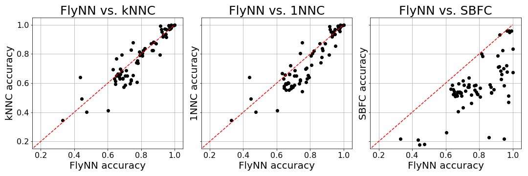
Figure 1: Performance of baselines relative to FlyNN on OpenML datasets. The scatter plots compare the best tuned FlyNN accuracy against that of $k$NNC, $1$NNC and SBFC with a point for each dataset, and the red dashed diagonal marking match to FlyNN accuracy.

Table 2: Evaluating FlyNN on OpenML datasets with (i) Fraction of datasets FlyNN outperforms baselines, (ii) Number of datasets FlyNN has wins(W)/ties(T)/losses(L) over baselines, (iii) Median improvement in normalized accuracy by FlyNN over baseline, (iv) $p$-values for the paired 2-sided t-test (TT), (v) $p$-values for the 2-sided Wilcoxon signed rank test (WSRT).

Method	(i) Frac.	(ii) W/T/L	(iii) Imp.	(iv) TT	(v) WSRT
$k$NNC	0.55	39/2/30	0.35%	5.30E-2	7.63E-2
$1$NNC	0.66	47/2/22	2.36%	1.55E-5	2.81E-5
SBFC	0.99	70/0/1	25.4%	$<$1E-8	$<$1E-8

We consider 70 classification (binary and multi-class) datasets from OpenML with $d$ numerical columns and $n$ samples; $d\in[20,1000],n\in[1000,20000]$. Unlike the synthetic sets, these datasets do not guarantee strong $k$NNC performance. The results are presented in Figure 1. In Table 2, the normalized accuracy of all baselines are compared to FlyNN with paired two-sided $t$-tests (TT) and two-sided Wilcoxon signed rank test (WSRT). In Figure 1, we can see on the left figure ($k$NNC vs FlyNN) that most points are near the diagonal (implying $k$NNC and FlyNN parity) with some under (better FlyNN accuracy) and some over (worse FlyNN accuracy). With $1$NNC in the center plot of Figure 1, we see that, in most cases, $1$NNC either matches FlyNN or does worse (being under the diagonal) since $k$NNC subsumes $1$NNC. But the right plot for SBFC in Figure 1 indicates that SBFC is quite unable to match FlyNN (and hence $k$NNC). We quantify these behaviours in Table 2. FlyNN performs comparably to $k$NNC (median improvement of only 0.35%) with $p$-values of $0.0536$ (TT) and 0.0763 (WSRT), while improving the normalized accuracy over $1$NNC by a median of around 2.36% across all 70 sets ($p$-values $\sim 10^{-5}$). These results demonstrate that the proposed FlyNN has comparable performance to properly tuned $k$NNC and this behaviour is verified with a large number of datasets. FlyNN significantly outperforms SBFC ($>25\%$ median improvement, $p$-values $<10^{-8}$), again highlighting the value of high sparsity in the FlyHash on real datasets.

Methods learned through gradient-descent (such as linear models or neural networks) have been widely studied in the FL setting. However, it is hard to compare nearest-neighbor methods against gradient-descent-based methods with proper parity. We present one comparison on these OpenML datasets in Appendix D.7.

Scaling.

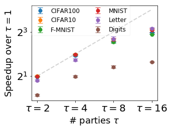
Figure 2: Scaling of FlyNNFL training with $\tau$ parties over single-party training. The gray line marks linear scaling.

We evaluate the scaling of the FlyNNFL training – Algorithm 2, TrainFlyNNFLDP – with the number of parties $\tau$. For fixed hyper-parameters, we average runtimes (and speedups) over 10 repetitions for each of the 6 datasets (see Appendix D.4) and present the results in Figure 2. The results indicate that TrainFlyNNFLDP scales very well for up to 8 parties for the larger datasets, and shows up to $8\times$ speed up with $16$ parties. There is significant gain (up to $2\times$) even for the tiny Digits dataset (with $<2000$ total rows), demonstrating the scalability of the FlyNN training with very low communication overhead.

Differential privacy.

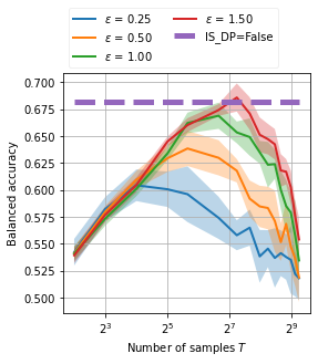
(a) Effect of $T$ for different $\epsilon$.

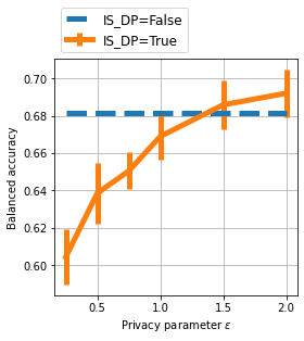
(b) Dependence on $\epsilon$.

Figure 3: The effect of the DP parameters $T$ and $\epsilon$ on the performance of FlyNNFL (higher is better).

To study the privacy-performance tradeoff of FlyNN, we again consider the previously described synthetic data in ${\mathbb{R}}^{d}$. For a fixed setting FlyNN hyper-parameters (namely $m,s,\rho,\gamma$) and 2-party federated training ($\tau=2$), we study the effect of the privacy parameters on FlyNNFL performance in Figure 3. In Figure 3(a), we see the effect of varying the number of sampled entries $T$. We observe the intuitive behaviour where, for a fixed privacy level $\epsilon$, increasing $T$ initially improves performance, but eventually hurts because of the high noise level obfuscating the FBF entries too drastically. In Figure 3(b), we report the effect of varying $\epsilon$. For each $\epsilon$, we select the $T$ corresponding to the best performance (based on Figure 3(a)). This shows the expected trend of increasing performance with increasing $\epsilon$, where the DP FlyNN can match the non-DP FlyNN (IS_DP=false) with $\epsilon$ close to 1. We present further experimental details and results for different dataset sizes and different FlyNN hyper-parameter configurations in Appendix D.8.

5 Related work

The $k$ nearest neighbor classification method ($k$NNC) is a conceptually simple, non-parametric and popular classification method which defers its computational burden to the prediction stage. The consistency properties of $k$NNC are well studied (Fix and Hodges 1951; Cover and Hart 1967; Devroye et al. 1994; Chaudhuri and Dasgupta 2014). Traditional $k$NNC assumes training data is stored centrally in a single machine, but such central processing and storing assumptions become unrealistic in the big data era. An effective way to overcome this issue is to distribute the data across multiple machines and use specific distributed computing environment such as Hadoop or Spark with MapReduce paradigm (Anchalia and Roy 2014; Mallio, Triguero, and Herrera 2015; Gonzalez-Lopez, Ventura, and Cano 2018). Zhang et al. (2020) proposed a $k$NNC algorithm based on the concept of distributed storage and computing for processing large datasets in cyber-physical systems where $k$-nearest neighbor search is performed locally using a kd-tree. Qiao, Duan, and Cheng (2019) analyzed a distributed $k$NNC in which data are divided into multiple smaller subsamples, $k$NNC predictions are made locally in each subsamples and these local predictions are combined via majority voting to make the final prediction. Securely computing $k$NNC is another closely related field when data is stored in different local devices. Majority of the frameworks that ensure privacy for $k$NNC often use some sort of secure multi-party computation (SMC) protocols (Zhan, Chang, and Matwin 2008; Xiong, Chitti, and Liu 2006; Qi and Atallah 2008; Schoppmann et al. 2020; Shaul, Feldman, and Rus 2020; Chen et al. 2020).

The federated learning framework involves training statistical models over remote devices while keeping data localized. Such a framework has recently received significant attention with the growth of the storage and computational capabilities of the remote devices within distributed networks especially because learning in such setting differs significantly from tradition distributed environment requiring advances in areas such as security and privacy, large-scale machine learning and distributed optimization. Excellent survey and research questions on this new field can be found in (Li et al. 2020; Kairouz and McMahan 2021). In federated learning, the parameters of a global model is learned in rounds, where in each round a central server sends the current state of the global algorithm (model parameters) to all the parties, each party makes local updates and sends the updates back to the central server (McMahan et al. 2017).

Current distributed $k$NNC schemes do not directly translate to the federated learning setting since the test point needs to be transmitted to all parties. In most secure $k$NNC settings considered in the literature, the goal is to keep the training data secure from the party making the test query (Qi and Atallah 2008; Shaul, Feldman, and Rus 2018; Wu et al. 2019) and it is not clear how those approaches extend to the multi-party federated setting where the per-party data (train or test) should remain localized. Of particular relevance is Schoppmann et al. (2020) which proposed a scheme to compute a secure inner-product between any test point and all training points (distributed across parties) and then perform a secure top-$k$ protocol to perform $k$NNC. This procedure explicitly computes the neighbors for a test point, which involves $n$ secure similarity computations for each test point (on top of the secure top-$k$ protocol). Both these steps require significant communication at inference time. In contrast, our proposed scheme do not require any explicit computation of the nearest-neighbors and hence requires no top-$k$ selection (secure or otherwise). In fact the inference requires no communication and the training can be made DP. Moreover, this paper focuses on document classification and leverages the significantly sparse feature representations of training examples. The high sparsity allows the use of correlated permutations to compute inner-products. However, the critical use of correlated permutations of the non-sparse indices augmented with padding does not translate to general dense data – in the absence of sparsity, the required correlated permutations would be very large and require multiple rounds of computation for a single similarity computation. Hence it is not clear if these techniques translate to the general $k$NNC.

6 Limitations & Future Work

A high-level limitation of our work is that we are not presenting a state-of-the-art result, but rather demonstrating how naturally occurring algorithms (FlyHash and FBF) can expand the scope of a canonical ML scheme (NNC) to more learning environments (FL). Our motivations are not to achieve state-of-the-art, but rather to explore and understand the novel unique capabilities of this neurobiological motif.

Another limitation is that the current theoretical connection between FlyNN and $k$NNC requires assumptions on the class margins and on the distribution of the data (the test point is from a permutation invariant distribution). This limits the scope of the theoretical result though we try to verify the theory with a large number of synthetic and real datasets. We plan to remove such assumptions in our future work.

Acknowledgement.

KS gratefully acknowledges funding from the “NSF AI Institute for Foundations of Machine Learning (IFML)” (FAIN: 2019844).

Appendix A Analyses of Algorithm 1 complexities

A.1 Proof for Lemma 1

Proof.

We can summarize the complexities for the different operations in TrainFlyNN (Algorithm 1) as follows:

• Line 2 takes $O(ms)$ time and memory to generate the random binary lifting matrix $\mathsf{M}$.

• Line 3 takes $O(mL)$ time and memory to initialize the per-class FBFs $\bm{w}_{l},l\in[L]$.

• Each FlyHash in line 5 takes $O(m(s+\log\rho))$ time and $O(m)$ memory.

• FBF $\bm{w}_{y}$ update in line 6 takes $O(\rho)$ time since $\gamma$ is multiplied to only $\rho$ entries in $\bm{w}_{y}$ since $\bm{\mathsf{h}}$ has only $\rho$ non-zero entries.

• Hence the loop 4-7 takes time $O(n(ms+m\log\rho+\rho))$ and maximum $O(m)$ additional memory.

• Given $\rho\ll m$ and $L\ll n$, the total runtime is given by $O(n\cdot m\cdot\max\{s,\log\rho\})$ time and $O(m\cdot\max\{s,L\})$ memory.

This proves the statement of the claim. ∎

A.2 Proof for Lemma 2

Proof.

We can summarize the complexities for the different operations in InferFlyNN (Algorithm 1) as follows:

• The FlyHash operation in line 11 takes time $O(m(s+\log\rho))$ and $O(m)$ memory.

• The operation in line 12 takes time $O(L\rho)$ since each $\bm{w}_{l}^{\top}\bm{\mathsf{h}}$ takes time $O(\rho)$ since $\bm{\mathsf{h}}$ only has $\rho$ nonzero entries and $O(L)$ additional memory.

• This leads to an overall runtime of $O(m\cdot\max\{s,\log\rho,(\rho L/m)\})$ and memory overhead of $O(\max\{m,L\})$.

This proves the statement of the claim. ∎

Appendix B Analysis of Algorithm 1 learning theoretic properties

B.1 Preliminaries & notations

We denote a single row of a lifting matrix $\mathsf{M}$ by $\theta\in\{0,1\}^{d}$ drawn i.i.d. from $Q$, the uniform distribution over all vectors in $\{0,1\}^{d}$ with exactly $s$ ones, satisfying $s\ll d$. We use an alternate formulation of the winner-take-all strategy as suggested in Dasgupta et al. (2018), where for any $\bm{x}\in{\mathbb{R}}^{d},\tau_{\bm{x}}$ is a threshold that sets largest $\rho$ entries of $\mathsf{M}\bm{x}$ to one (and the rest to zero) in expectation. Specifically, for a given $\bm{x}\in{\mathbb{R}}^{d}$ and for any fraction $0<f<1$, we define $\tau_{\bm{x}}(f)$ to be the top $f$-fractile value of the distribution $\theta^{\top}\bm{x}$, where $\theta\sim Q$:

$$\tau_{\bm{x}}(f)=\sup\{v:{\mathop{\rm Pr}}_{\theta\sim Q}(\theta^{\top}\bm{x}\geq v)\geq f\}$$ (3)

We note that for any $0<f<1$, ${\mathop{\rm Pr}}_{\theta\sim Q}(\theta^{\top}\bm{x}\geq\tau_{\bm{x}}(f))\approx f$, where the approximation arises from possible discretization issues. For convenience, henceforth we will assume that this is an equality:

$${\mathop{\rm Pr}}_{\theta\sim Q}(\theta^{\top}\bm{x}\geq\tau_{\bm{x}}(f))=f$$ (4)

For any two $\bm{x},\bm{x}^{\prime}\in{\mathbb{R}}^{d}$, we define $q(\bm{x},\bm{x}^{\prime})={\mathop{\rm Pr}}_{\theta\sim Q}\left(\theta^{\top}\bm{x}^{\prime}\geq\tau_{\bm{x}^{\prime}}\left(\rho/m\right)~{}|~{}\theta^{\top}\bm{x}\geq\tau_{\bm{x}}\left(\rho/m\right)\right)$. This can be interpreted as follows – with $\bm{\mathsf{h}}=h(\bm{x}),\bm{\mathsf{h}}^{\prime}=h(\bm{x}^{\prime})$ as the FlyHashes of $\bm{x}$ and $\bm{x}^{\prime}$, respectively, $q(\bm{x},\bm{x}^{\prime})$ is the probability that $\bm{\mathsf{h}}^{\prime}[j]=1$ given that $\bm{\mathsf{h}}[j]=1$, for any specific $j\in[m]$.

We begin by analyzing the binary classification performance of FlyNN trained on a training set $S=\{(\bm{x}_{i},y_{i})\}_{i=1}^{n_{0}+n_{1}}\subset{\mathbb{R}}\times\{0,1\}$, where $S=S^{1}\cup S^{0}$, $S^{0}$ is a subset of $S$ having label 0, and $S^{1}$ is a subset of $S$ having label 1, satisfying $|S^{0}|=n_{0}$, $|S^{1}|=n_{1}$ and $n=n_{0}+n_{1}$. For appropriate choice of $m$, let $\bm{w}_{0},\bm{w}_{1}\in\{0,1\}^{m}$ be the FBFs constructed using $S^{0}$ and $S_{1}$ respectively.

B.2 Connection to $k$NNC

We first present the following lemmas which will be required to prove Theorem 3.

Lemma 7 (Expected novelty response (Dasgupta et al. 2018)).

Suppose that inputs $\bm{x}_{1},\ldots,\bm{x}_{n}\in{\mathbb{R}}^{d}$ are first presented with $\bm{x}_{i}\rightarrow\bm{y}_{i}\rightarrow\mathsf{h}_{i}$, where $\bm{y}_{i}=\mathsf{M}\bm{x}_{i},\mathsf{h}_{i}=h(\bm{x}_{i})$, and $\bm{w}$ is the FBF constructed using $\bm{x}_{1},\ldots,\bm{x}_{n}$. Then a subsequent input $\bm{x}$ is presented with $\bm{x}\rightarrow\bm{y}\rightarrow\mathsf{h}$, where $\bm{y}=\mathsf{M}\bm{x},\mathsf{h}=h(\bm{x})$.

(a) The $m$ random vectors $(\bm{y}_{1}[j],\ldots,\bm{y}_{n}[j],\mathsf{h}_{1}[j],\ldots,\mathsf{h}_{n}[j],\bm{y}[j],\mathsf{h}[j],\bm{w}[j]),1\leq j\leq m$, (over the random choice choice of $\mathsf{M}$) are independent and identically distributed.

(b) The novelty response to $\bm{x}$ has expected value

$$\mu={{\mathbb{E}}}(\bm{w}^{\top}h(\bm{x})/\rho)={\mathop{\rm Pr}}_{\theta\sim Q}\left(\theta^{\top}\bm{x}_{1}<\tau_{\bm{x}_{1}},\ldots,\theta^{\top}\bm{x}_{n}<\tau_{\bm{x}_{n}}~{}|~{}\theta^{\top}\bm{x}\geq\tau_{\bm{x}}\right)$$

Lemma 8 (Bounds on expected novelty response (Dasgupta et al. 2018)).

The expected value $\mu$ from Lemma 7 can be bounded as follows:

(a) Lower bound: $\mu\geq 1-\sum_{i=1}^{n}q(\bm{x},\bm{x}_{i})$.

(b) Upper bound: for any $1\leq l\leq n$, $~{}~{}\mu\leq 1-q(\bm{x},\bm{x}_{l})$.

Lemma 9 ((Dasgupta et al. 2018)).

Pick any $\bm{x},\bm{x}^{\prime}\in{\mathbb{R}}^{d}$. Suppose that for all $i\in[d]$, $\bm{x}^{\prime}[i]\geq\bm{x}[i]-\Delta/s$, where $\Delta=\frac{1}{2}\left(\tau_{\bm{x}}(\rho/2m)-\tau_{\bm{x}}(\rho/m)\right)$. then $q(\bm{x},\bm{x}^{\prime})\geq 1/2$.

Corollary 10 ((Dasgupta et al. 2018)).

Fix any $\bm{x}^{\prime}\in{\mathbb{R}}^{d}$ and pick $\bm{x}$ from any permutation invariant distribution over ${\mathbb{R}}^{d}$. then the expected value of $q(\bm{x},\bm{x}^{\prime})$, over the choice of $\bm{x}$ is $\rho/m$.

Lemma 11.

Fix any $\bm{x}\in{\mathbb{R}}^{d}$ and let $h(\bm{x})\in\{0,1\}^{m}$ be its FlyHash using equation 2. For any integer $k$, let $\bm{x}_{*}^{i}$ be the $\left(\lceil\frac{k+1}{2}\rceil\right)^{th}$ nearest neighbor of $\bm{x}$ in $S^{i}$ measured using $\ell_{\infty}$ metric. Let $A_{S^{1}}=\{\theta:\cap_{(\bm{x}^{\prime},y^{\prime})\in S^{1}}~{}\theta^{\top}\bm{x}^{\prime}<\tau_{\bm{x}^{\prime}}(\rho/m)\}$ and $A_{S^{0}}=\{\theta:\cap_{(\bm{x}^{\prime},y^{\prime})\in S^{0}}~{}\theta^{\top}\bm{x}^{\prime}<\tau_{\bm{x}^{\prime}}(\rho/m)\}$. Then the following holds, where the expectation is taken over the random choice of projection matrix $\mathsf{M}$.
(i) ${{\mathbb{E}}}_{\mathsf{M}}(\frac{\bm{w}_{1}^{\top}h(\bm{x})}{\rho})={\mathop{\rm Pr}}_{\theta\sim Q}\left(A_{S^{1}}~{}|~{}\theta^{\top}\bm{x}\geq\tau_{\bm{x}}(\rho/m)\right)$
(ii) ${{\mathbb{E}}}_{\mathsf{M}}(\frac{\bm{w}_{0}^{\top}h(\bm{x})}{\rho})={\mathop{\rm Pr}}_{\theta\sim Q}\left(A_{S^{0}}~{}|~{}\theta^{\top}\bm{x}\geq\tau_{\bm{x}}(\rho/m)\right)$
(iii) ${{\mathbb{E}}}_{\mathsf{M}}(\frac{\bm{w}_{1}^{\top}h(\bm{x})}{\rho})\geq 1-\sum_{\bm{x}^{\prime}\in S^{1}}q(\bm{x},\bm{x}^{\prime})$
(iv) ${{\mathbb{E}}}_{\mathsf{M}}(\frac{\bm{w}_{1}^{\top}h(\bm{x})}{\rho})\leq 1-q(\bm{x},\bm{x}_{*}^{1})$
(v) ${{\mathbb{E}}}_{\mathsf{M}}(\frac{\bm{w}_{0}^{\top}h(\bm{x})}{\rho})\geq 1-\sum_{\bm{x}^{\prime}\in S^{0}}q(\bm{x},\bm{x}^{\prime})$
(vi) ${{\mathbb{E}}}_{\mathsf{M}}(\frac{\bm{w}_{0}^{\top}h(\bm{x})}{\rho})\leq 1-q(\bm{x},\bm{x}_{*}^{0})$

Proof.

Part (i) and (ii) follows from simple application of Lemma 7 to class specific FBFs. Part (iii) and (v) follows from simple application of Lemma 8 to class specific FBFs. For part (iv), simple application of Lemma 8 to FBF $\bm{w}_{1}$ ensures that for any $\bm{x}^{\prime}\in S^{1},{{\mathbb{E}}}_{\mathsf{M}}(\frac{\bm{w}_{1}^{\top}h(\bm{x})}{\rho})\leq 1-q(\bm{x},\bm{x}^{\prime})$. Clearly, ${{\mathbb{E}}}_{\mathsf{M}}(\frac{\bm{w}_{1}^{\top}h(\bm{x})}{\rho})\leq 1-q(\bm{x},\bm{x}_{*}^{1})$. Applying similar argument, part (vi) also holds. ∎

Lemma 12.

Let $\bm{w}_{0}$ and $\bm{w}_{1}$ be the FBFs constructed using $S^{0}$ and $S^{1}$. For any $\bm{x}\in{\mathbb{R}}^{d}$ let $\mu_{0}={{\mathbb{E}}}_{\mathsf{M}}\left(\frac{\bm{w}_{0}^{\top}h(\bm{x})}{\rho}\right)$ and $\mu_{1}={{\mathbb{E}}}_{\mathsf{M}}\left(\frac{\bm{w}_{1}^{\top}h(\bm{x})}{\rho}\right)$ Then, for any $\epsilon>0$ the following holds,
(i) ${\mathop{\rm Pr}}\left(\frac{\bm{w}_{1}^{\top}h(\bm{x})}{\rho}\geq(1+\epsilon)\mu_{1}\right)\leq\exp(-\epsilon^{2}\rho\mu_{1}/3)$
(ii) ${\mathop{\rm Pr}}\left(\frac{\bm{w}_{0}^{\top}h(\bm{x})}{\rho}\geq(1+\epsilon)\mu_{0}\right)\leq\exp(-\epsilon^{2}\rho\mu_{0}/3)$
(iii) ${\mathop{\rm Pr}}\left(\frac{\bm{w}_{1}^{\top}h(\bm{x})}{\rho}\leq(1-\epsilon)\mu_{1}\right)\leq\exp(-\epsilon^{2}\rho\mu_{1}/2)$
(iii) ${\mathop{\rm Pr}}\left(\frac{\bm{w}_{0}^{\top}h(\bm{x})}{\rho}\leq(1-\epsilon)\mu_{0}\right)\leq\exp(-\epsilon^{2}\rho\mu_{0}/2)$

Proof.

We will only prove part (i) since part (ii) is similar. Let $\bm{\mathsf{h}}=h(\bm{x}),\bm{\mathsf{h}}_{1}=h(\bm{x}_{1}),\ldots,\bm{\mathsf{h}}_{n_{1}}=h(\bm{x}_{n_{1}})$ be the FlyHashes of $\bm{x},\bm{x}_{1},\ldots,\bm{x}_{n_{1}}$ that belongs to $S^{1}$. Define random variables $U_{1},\ldots,U_{m}\in\{0,1\}$ as follows:

$$U_{j}=\begin{cases}1,&\text{if }\bm{\mathsf{h}}_{1}[j]=\cdots=\bm{\mathsf{h}}_{n_{1}}[j]=0\text{ and }\bm{\mathsf{h}}[j]=1\\ 0,&\text{otherwise}\end{cases}$$

The $U_{j}$ are i.i.d. and

$${{\mathbb{E}}}_{\mathsf{M}}(U_{j}) = {\mathop{\rm Pr}}_{\mathsf{M}}(\bm{\mathsf{h}}[j]=1)\times$$

$${\mathop{\rm Pr}}_{\mathsf{M}}\left(\bm{\mathsf{h}}_{1}[j]=\cdots=\bm{\mathsf{h}}_{n_{1}}[j]=0~{}|~{}\bm{\mathsf{h}}[j]=1\right)$$

$$= \frac{\rho}{m}{{\mathbb{E}}}_{\mathsf{M}}\left(\frac{\bm{w}_{1}^{\top}h(\bm{x})}{\rho}\right)$$

where we have used the fact that ${\mathop{\rm Pr}}_{\mathsf{M}}(h(\bm{x})_{j}=1)={\mathop{\rm Pr}}_{\theta\sim Q}(\theta^{\top}\bm{x}\geq\tau_{\bm{x}}(\rho/m))=\rho/m$ and using Lemma 2 of the supplementary material of (Dasgupta et al. 2018), ${\mathop{\rm Pr}}_{\mathsf{M}}\left(\bm{\mathsf{h}}_{1}[j]=\cdots=\bm{\mathsf{h}}_{n_{1}}[j]=0~{}|~{}\bm{\mathsf{h}}[j]=1\right)={{\mathbb{E}}}_{\mathsf{M}}\left(\frac{\bm{w}_{1}^{\top}h(\bm{x})}{\rho}\right)$. Therefore, ${{\mathbb{E}}}_{\mathsf{M}}(U_{1}+\cdots+U_{m})=\rho\cdot{{\mathbb{E}}}_{\mathsf{M}}\left(\frac{\bm{w}_{1}^{\top}h(\bm{x})}{\rho}\right)$. Let $\mu_{1}={{\mathbb{E}}}_{\mathsf{M}}\left(\frac{\bm{w}_{1}^{\top}h(\bm{x})}{\rho}\right)$. By multiplicative Chernoff bound for any $0<\epsilon<1$, we have,

$${\mathop{\rm Pr}}_{M}\left(U_{1}+\cdots+U_{m}\geq(1+\epsilon)\rho\mu_{1}\right) \leq\exp(-\epsilon^{2}\rho\mu_{1}/3)$$

$${\mathop{\rm Pr}}_{M}\left(U_{1}+\cdots+U_{m}\leq(1-\epsilon)\rho\mu_{1}\right) \leq\exp(-\epsilon^{2}\rho\mu_{1}/2)$$

Noticing that $U_{1}+\cdots+U_{m}=\bm{w}_{1}^{\top}h(\bm{x})$, the result follows. ∎

B.3 Proof of Theorem 3

Proof.

Without loss of generality, assume that $k$NNC prediction of $\bm{x}$ is 1. For the case when $k$NNC prediction is 0 is similar. Prediction of FlyNN on $\bm{x}$ agrees with the prediction of $k$NNC whenever $\left(\bm{w}_{1}^{\top}h(\bm{x})/\rho\right)<\left(\bm{w}_{0}^{\top}h(\bm{x})/\rho\right)$. We first show that ${{\mathbb{E}}}_{\mathsf{M}}\left(\bm{w}_{1}^{\top}h(\bm{x})/\rho\right)<{{\mathbb{E}}}_{\mathsf{M}}\left(\bm{w}_{0}^{\top}h(\bm{x})/\rho\right)$ with high probability and then using standard concentration bound presented in lemma 12, we achieve the desired result.

Since $\|\bm{x}-\bm{x}_{*}\|\leq\frac{\eta}{2}$, all the $\lceil\frac{k+1}{2}\rceil$ nearest neighbors of $\bm{x}$ have same label. Let $\|\bm{x}-\bm{x}_{*}\|_{\infty}\leq\Delta/s$, where $\Delta=\frac{1}{2}\left(\tau_{\bm{x}}(\rho/2m)-\tau_{\bm{x}}(\rho/m)\right)$. Using lemma 9, we get $q(\bm{x},\bm{x}_{*})\geq 1/2$. Combining this with part (iv) of lemma 11, we get $\mu_{1}={{\mathbb{E}}}_{\mathsf{M}}\left(\bm{w}_{1}^{\top}h(\bm{x})/\rho\right)\leq 1-q(\bm{x},\bm{x}^{*})\leq 1/2$.

If $\bm{x}$ is sampled from a permutation invariant distribution, using corollary 10, we get ${{\mathbb{E}}}_{\bm{x}}q(\bm{x},\bm{x}_{i})=\rho/m$ for each $\bm{x}^{\prime}\in S^{0}$, and thus using linearity of expectation, ${{\mathbb{E}}}_{\bm{x}}\left(\sum_{\bm{x}^{\prime}\in S^{0}}q(\bm{x},\bm{x}^{\prime})\right)=\sum_{\bm{x}^{\prime}\in S^{0}}{{\mathbb{E}}}_{\bm{x}}q(\bm{x},\bm{x}^{\prime})=\rho n_{0}/m$. For any $\alpha>0$, using Markov’s inequality,

$$pr\left(\sum_{\bm{x}^{\prime}\in S^{0}}q(\bm{x},\bm{x}^{\prime})>\alpha\right)\leq\frac{{{\mathbb{E}}}_{\bm{x}}\left(\sum_{\bm{x}^{\prime}\in S^{0}}q(\bm{x},\bm{x}^{\prime}\right)}{\alpha}=\frac{\rho n_{0}}{m\alpha}.$$ (5)

Specifically, choose $\alpha=1/4$. Then with probability $\geq 1-\frac{4\rho n_{0}}{m}$, we have $\sum_{\bm{x}^{\prime}\in S^{0}}q(\bm{x},\bm{x}^{\prime})\leq\frac{1}{4}$. Combining this with part (v) of lemma 11, we immediately get, with probability $\geq 1-\frac{4\rho n_{0}}{m}$, we have $\mu_{0}={{\mathbb{E}}}_{\mathsf{M}}\left(\bm{w}_{0}^{\top}h(\bm{x})/\rho\right)\geq 3/4$.

Next we show that $\frac{\bm{w}_{1}^{\top}h(\bm{x})}{\rho}\leq 3/5$ with high probability.

If we set $\epsilon=\frac{1}{10\mu_{1}}$, then we get $(1+\epsilon)\mu_{1}=\mu_{1}+\epsilon\mu_{1}\leq\frac{1}{2}+\epsilon\mu_{1}=\frac{1}{2}+\frac{1}{10}=\frac{3}{5}$. For this choice of $\epsilon$, $\mu_{1}(1+\epsilon)\leq 3/5$. Therefore,

$${\mathop{\rm Pr}}\left(\frac{w_{1}^{\top}h(\bm{x})}{\rho}>3/5\right) \leq {\mathop{\rm Pr}}\left(\frac{w_{1}^{\top}h(\bm{x})}{\rho}>(1+\epsilon)\mu_{1}\right)$$

$$\leq \exp(-\epsilon^{2}\rho\mu_{1}/3)$$

$$= \exp\left(-\frac{\rho}{300\mu_{1}}\right)$$

$$\leq \exp\left(-\frac{\rho}{150}\right)$$

where the first inequality follows from our choice of $\epsilon$, the second inequality follows from Lemma 12, the equality follows from our choice of $\epsilon$ and the third inequality follows since $\mu_{1}\leq\frac{1}{2}$.

Next, we would like to show $\frac{\bm{w}_{0}^{\top}h(\bm{x})}{\rho}\geq\frac{5}{8}>\frac{3}{5}$ with high probability. If we set set $\epsilon_{1}=\frac{1}{6}$ and using the fact that $\mu_{0}\geq\frac{3}{4}$, we get $(1-\epsilon_{1})\mu_{0}=\frac{5}{6}\mu_{0}\geq\frac{5}{6}\cdot\frac{3}{4}=\frac{5}{8}$.

Now we have,

$${\mathop{\rm Pr}}\left(\frac{w_{0}^{\top}h(\bm{x})}{\rho}<5/8\right) \leq {\mathop{\rm Pr}}\left(\frac{w_{0}^{\top}h(\bm{x})}{\rho}<(1-\epsilon_{1})\mu_{1}\right)$$

$$\leq \exp(-\epsilon^{2}\rho\mu_{0}/2)$$

$$= \exp\left(-\frac{\rho\mu_{0}}{72}\right)$$

$$\leq \exp\left(-\frac{\rho}{96}\right)$$

where the first inequality follows from our choice of $\epsilon_{1}$, the second inequality follows from Lemma 12, the equality follows again from our choice of $\epsilon_{1}$ and the third inequality follows from the fact that $\mu_{1}\leq 1$.

Therefore, with probability at least $1-\left(\frac{4\rho n_{0}}{m}+e^{-\frac{\rho}{150}}+e^{-\frac{\rho}{96}}\right)$ we have, (i) $\frac{\bm{w}_{0}^{\top}h(\bm{x})}{\rho}\geq\frac{5}{8}$, and (ii) $\frac{3}{5}\geq\frac{\bm{w}_{1}^{\top}h(\bm{x})}{\rho}$. Since $\frac{5}{8}>\frac{3}{5}$, the result follows. ∎

Appendix C Analyses for Algorithm 2

The proofs for all the theoretical results in §3 are presented in this section.

C.1 Proof of Theorem 4

Proof.

Given the per-party data chunk $S_{t},t\in[\tau]$, let us consider the FBF $\bm{w}_{l}\in(0,1)^{m}$ for any class $l\in[L]$ learned over the pooled data $S=\cup_{t\in[\tau]}S_{t}$ using the TrainFlyNN subroutine in Algorithm 1. For any $i\in[m]$ and $l\in[L]$:

$$\bm{w}_{l}[i] =1\cdot\underbrace{\gamma\cdot\gamma\cdot\cdots\cdot\gamma}_{\text{\# times }\bm{\mathsf{h}}[i]=1\text{ for some }(\bm{x},y)\in S,y=l}$$

$$=\gamma^{\left|\left\{(\bm{x},y)\in S:y=l,\bm{\mathsf{h}}=\Gamma_{\rho}(\mathsf{M}\bm{x}),\bm{\mathsf{h}}[i]=1\right\}\right|}.$$ (6)

By the same argument, the FBF $\bm{w}_{l}^{t}$ learned with data chunk $S_{t}$ for a class $l$ (Algorithm 2, line 4) can be summarized as follows for any $i\in[m]$:

$$\bm{w}_{l}^{t}[i] =\gamma^{\left|\left\{(\bm{x},y)\in S_{t}:y=l,\bm{\mathsf{h}}=\Gamma_{\rho}(\mathsf{M}\bm{x}),\bm{\mathsf{h}}[i]=1\right\}\right|}.$$ (7)

Then the all-reduced FBF $\hat{\bm{w}}_{l}$ for a class $l$ (Algorithm 2, line 9) is given by the following for any $i\in[m]$:

$$\hat{\bm{w}}_{l}[i] =\gamma^{\sum_{t\in[\tau]}\log_{\gamma}\bm{w}_{l}^{t}[i]}$$ (8)

$$\stackrel{{\scriptstyle(A)}}{{=}}\gamma^{\sum_{t\in[\tau]}\left|\left\{(\bm{x},y)\in S_{t}:y=l,\bm{\mathsf{h}}=\Gamma_{\rho}(\mathsf{M}\bm{x}),\bm{\mathsf{h}}[i]=1\right\}\right|}$$ (9)

$$\stackrel{{\scriptstyle(B)}}{{=}}\gamma^{\left|\cup_{t\in[\tau]}\left\{(\bm{x},y)\in S_{t}:y=l,\bm{\mathsf{h}}=\Gamma_{\rho}(\mathsf{M}\bm{x}),\bm{\mathsf{h}}[i]=1\right\}\right|}$$ (10)

$$\stackrel{{\scriptstyle(C)}}{{=}}\gamma^{\left|\left\{(\bm{x},y)\in\underbrace{\cup_{t\in[\tau]}S_{t}}_{S}:y=l,\bm{\mathsf{h}}=\Gamma_{\rho}(\mathsf{M}\bm{x}),\bm{\mathsf{h}}[i]=1\right\}\right|}$$ (11)

$$=\gamma^{\left|\left\{(\bm{x},y)\in S:y=l,\bm{\mathsf{h}}=\Gamma_{\rho}(\mathsf{M}\bm{x}),\bm{\mathsf{h}}[i]=1\right\}\right|}$$ (12)

$$\stackrel{{\scriptstyle(D)}}{{=}}\bm{w}_{l}[i],$$ (13)

where $(A)$ is obtained from (7), $(B)$ is obtained from the fact that the sets $S_{t},t\in[\tau]$ are disjoint (no data shared between parties), $(C)$ is from the fact that a union of subsets of disjoint sets ($S_{t}$) is the same as a subset of union of disjoint sets $\cup_{t}S_{t}$. $(D)$ follows from (6).

Since the above holds for all $i\in[m]$, we can say that $\bm{w}_{l}=\hat{\bm{w}}_{l}\forall l\in[L]$, proving the statement of the claim. ∎

C.2 Proof of Lemma 5

Proof.

We begin with recalling that the all-reduce operation can be performed efficiently in a peer-to-peer communication setup where the $\tau$ parties can be organized as a binary tree of depth $O(\log\tau)$. Then the communication at each level of the tree can be done in parallel for each independent subtree at that level. Consider the object being all-reduced to be of size $O(c)$. Then in the first round of communication, $O(\tau/2)$ pairs of parties combine their objects in parallel in time $O(c)$ with total communication $O(c\tau/2)$ and $O(c)$ memory overhead in each of the parties. In the second round, $O(\tau/4)$ pairs of parties combine their objects in parallel again in time $O(c)$ with total communication $O(c\tau/4)$ with $O(c)$ memory overhead in $O(\tau/2)$ of the parties. Going up the tree to the root then takes time $O(c\log\tau)$. The total communication cost is $O(c\tau)$.

The communication first goes bottom up from the leaves to the root, which then has the final all-reduced result. Then this result is sent to each party top-down from the root (in a corresponding manner) so that eventually all parties have the all-reduced result in time $O(c\log\tau)$ with total $O(c\tau)$ communication.

Based on the above complexities of the all-reduce operation, we can summarize the complexities for the different operations in TrainFlyNNFLDP (Algorithm 2) when DP is disabled ($\tt{IS\_DP}=false$) as follows:

• The broadcast of the random seed in line 2 can be done with an all-reduce in $O(\log\tau)$ time and $O(\tau)$ total communication and $O(1)$ memory overhead in each party.

• On party $V_{t}$, the invocation of TrainFlyNN in line 4 on data chunk $S_{t}$ of size $n_{t}$ takes $O(n_{t}\cdot m\cdot\max\{s,\log\rho\})$ time and $O(m\cdot\max\{s,L\})$ memory from Lemma 1 and no communication cost.

• The all-reduce of the per-party per-class FBFs in line 9 takes time $O(m\cdot L\cdot\log\tau)$ with $O(m\cdot L\cdot\tau)$ total communication, and $O(m\cdot L)$ memory overhead per-party.

Putting them all together gives us the per-party time complexity of $O(n_{t}\cdot m\cdot\max\{s,\log\rho,(L/n_{t})\log\tau\})$, memory overhead of $O(m\cdot\max\{s,L\})$ and total communication among all parties of $O(m\cdot L\cdot\tau)$, giving us the statement of the claim.

When DP is enabled ($\tt{IS\_DP}=true$), we can summarize the complexity of various operations as follows,

• The broadcast of the random seed in line 2 can be done with an all-reduce in $O(\log\tau)$ time and $O(\tau)$ total communication and $O(1)$ memory overhead in each party.

• On party $V_{t}$, the invocation of TrainFlyNN in line 4 on data chunk $S_{t}$ of size $n_{t}$ takes $O(n_{t}\cdot m\cdot\max\{s,\log\rho\})$ time and $O(m\cdot\max\{s,L\})$ memory from Lemma 1 and no communication cost.

• On party $V_{t}$, the invocation of DP subroutine in line 6 takes $O(m\cdot L\cdot T)$ time, $O(m\cdot L)$ memory and requires no communication cost.

• The all-reduce of the per-party per-class FBFs in line 9 takes time $O(T\cdot\log\tau)$ with $O(T\cdot\tau)$ total communication, and $O(m\cdot L)$ memory overhead per-party.

Putting them all together gives us the per-party time complexity of $O(n_{t}\cdot m\cdot\max\{s,\log\rho,(LT/n_{t})\}+T\cdot\log\tau)$, memory overhead of $O(m\cdot\max\{s,L\})$ and total communication among all parties of $O(T\cdot\tau)$, giving us the statement of the claim. ∎

C.3 Proof of Theorem 6

Proof.

Let $\epsilon_{0}=\frac{\epsilon}{2T\tau}$. Note that a single data point (record) $\bm{x}$ can affect a single FBF corresponding to its own class labels located at a fixed party. For any pair of neighboring databases $D$ and $\bar{D}$ that differ in a single record, let $\bm{c}$ and $\bar{\bm{c}}$ be the respective count vectors (concatenating $L$ count vectors, one per class label). Then for any $i\in[m\times L],~{}|\bm{c}[i]-\bar{\bm{c}}[i]|\leq 1$. Fix any party $t\in[\tau]$ and any iteration $j\in[T]$. In line 17 of Algorithm 2, $i_{j}$ is sampled using the exponential mechanism in iteration $j$, therefore using standard properties of exponential mechanism, releasing the index $i_{j}$ is $\epsilon_{0}$ differentially private. Next using the property of Laplace mechanism, releasing the value at the $i_{j}^{th}$ index, i.e., $\bm{c}[i_{j}]$ (in line 18-19 of Algorithm 2) is $\epsilon_{0}$ differentially private. Therefore, releasing the count $\bm{c}[i_{j}]$ is $\epsilon_{0}+\epsilon_{0}=2\epsilon_{0}=\frac{\epsilon}{T\tau}$ difefrentially private. Applying the composition theorem over all $t\in[\tau]$ and $j\in[T]$, TrainFlyNNFLDP is $(\epsilon,0)$ differentially private. ∎

Appendix D Empirical evaluations

D.1 Implementation & Compute Resources details

The proposed FlyNN is implemented in Python 3.6 to fit the scikit-learn API (Pedregosa et al. 2011), but the current implementation is not optimized for computational performance. We use the scikit-learn implementation of $k$NNC. The experiments are performed on a 16-core 128GB machine running Ubuntu 18.04. The code is available at https://github.com/rithram/flynn.

D.2 Synthetic data description

We consider synthetic data of varying sizes and properties. These synthetic data are designed in a way that favors local classifiers such as the nearest-neighbor classifiers – each class conditional data distribution consists of multiple separated modes, with enough separation between modes of different classes (Guyon 2003). We consider 5 classes with 3 modes per class. These data are balanced in the class sizes and have no labeling noise. We consider these synthetic data to see if our proposed FlyNN is able to capture multiple separated local class neighborhoods in a single per-class FBF encoding while providing enough separation between FBFs of different classes to have strong classification performance. To generate synthetic datasets, we use the data.make_classification functionality (Guyon 2003) in scikit-learn (Pedregosa et al. 2011).

We also study the effect of the number of non-zeros $b<d$ in the binary data on the performance of FlyNN and baselines. The results indicate that, for fixed data dimensionality $d$, the relative performance of FlyNN is not significantly affected by the choice of $b<d$. The performance of SBFC seems to improve with increasing $b$.

Table 3: Comparison of FlyNN with nearest neighbor classifiers and SBFC on synthetic data. For binary data $\mathcal{X}=\{0,1\}^{d}$, we try different values of number of non-zeros $b<d$, denoted by different values of $|x|=b,x\in\mathcal{X}$. We report the normalized accuracy aggregated over 30 random synthetic datasets. Normalized accuracy of $k$NNC is zero hence not present in the table.

$\mathcal{X}$	$n$	$d$	SBFC	FlyNN
$\{0,1\}^{d},|x|=10$	$10^{3}$	$100$	$0.63\pm 0.02$	$-0.06\pm 0.02$
$\{0,1\}^{d},|x|=20$	$10^{3}$	$100$	$0.58\pm 0.03$	$-0.04\pm 0.02$
$\{0,1\}^{d},|x|=30$	$10^{3}$	$100$	$0.29\pm 0.04$	$-0.03\pm 0.02$
$\{0,1\}^{d},|x|=40$	$10^{3}$	$100$	$0.18\pm 0.03$	$-0.03\pm 0.02$

D.3 OpenML data details

We consider OpenML datasets utilizing the following query for OpenML classification datasets with no categorical and missing features with number of features $d\in[20,1000]$, number of rows $n\in[1000,20000]$ and number of classes $L\in[2,30]$, leading to $70$ data sets where there were no issues with the data retrieval and the processing of the data with scikit-learn operators.

We deliberately chose a large set of datasets to evaluate how generally FlyNN is able to mimic $k$NNC. While our theoretical guarantees require certain margin conditions, we wanted to look at a wide variety of datasets where such conditions may or may not be satisfied and understand the true empirical behaviour of FlyNN relative to $k$NNC.

OpenML query for datasets.

We use the following code snippet to obtain the list of datasets we try. Details on the precise 70 datasets we used is presented in Table 4.

⬇

1from openml.datasets import list_datasets, get_dataset

2openml_df = list_datasets(output_format=’dataframe’)

3val_dsets = openml_df.query(

4 ’NumberOfInstancesWithMissingValues == 0 & ’

5 ’NumberOfMissingValues == 0 & ’

6 ’NumberOfClasses > 1 & ’

7 ’NumberOfClasses <= 30 & ’

8 ’NumberOfSymbolicFeatures == 1 & ’

9 ’NumberOfInstances > 999 &’

10 ’NumberOfFeatures >= 20 &’

11 ’NumberOfFeatures <= 1000 &’

12 ’NumberOfInstances <= 20000’

13)[[

14 ’name’, ’did’, ’NumberOfClasses’,

15 ’NumberOfInstances’, ’NumberOfFeatures’

16]]

Table 4: OpenML datasets used in this evaluation.

Name	OpenML ID	$L$	$n$	$d$
mfeat-fourier	14	10	2000	77
mfeat-karhunen	16	10	2000	65
mfeat-zernike	22	10	2000	48
optdigits	28	10	5620	65
spambase	44	2	4601	58
waveform-5000	60	3	5000	41
satimage	182	6	6430	37
fri-c3-1000-25	715	2	1000	26
fri-c4-1000-100	718	2	1000	101
pol	722	2	15000	49
fri-c4-1000-25	723	2	1000	26
ailerons	734	2	13750	41
puma32H	752	2	8192	33
cpu-act	761	2	8192	22
fri-c4-1000-50	797	2	1000	51
fri-c3-1000-50	806	2	1000	51
bank32nh	833	2	8192	33
fri-c1-1000-50	837	2	1000	51
fri-c0-1000-25	849	2	1000	26
fri-c2-1000-50	866	2	1000	51
fri-c2-1000-25	903	2	1000	26
fri-c0-1000-50	904	2	1000	51
fri-c1-1000-25	917	2	1000	26
mfeat-fourier	971	2	2000	77
waveform-5000	979	2	5000	41
optdigits	980	2	5620	65
mfeat-zernike	995	2	2000	48
mfeat-karhunen	1020	2	2000	65
pc4	1049	2	1458	38
pc3	1050	2	1563	38
kc1	1067	2	2109	22
pc1	1068	2	1109	22
PizzaCutter3	1444	2	1043	38
PieChart3	1453	2	1077	38
cardiotocography	1466	10	2126	36
first-order-theorem-proving	1475	6	6118	52
hill-valley	1479	2	1212	101
ozone-level-8hr	1487	2	2534	73
qsar-biodeg	1494	2	1055	42
ringnorm	1496	2	7400	21
wall-robot-navigation	1497	4	5456	25
steel-plates-fault	1504	2	1941	34
twonorm	1507	2	7400	21
autoUniv-au1-1000	1547	2	1000	21
cardiotocography	1560	3	2126	36
hill-valley	1566	2	1212	101
GesturePhaseSegmentationProcessed	4538	5	9873	33
thyroid-ann	40497	3	3772	22
texture	40499	11	5500	41
Satellite	40900	2	5100	37
steel-plates-fault	40982	7	1941	28
sylvine	41146	2	5124	21
ada	41156	2	4147	49
microaggregation2	41671	5	20000	21
Sick-numeric	41946	2	3772	30
mfeat-factors	12	10	2000	217
isolet	300	26	7797	618
mfeat-factors	978	2	2000	217
gina-agnostic	1038	2	3468	971
gina-prior2	1041	10	3468	785
gina-prior	1042	2	3468	785
cnae-9	1468	9	1080	857
madelon	1485	2	2600	501
semeion	1501	10	1593	257
clean2	40666	2	6598	169
Speech	40910	2	3686	401
mfeat-pixel	40979	10	2000	241
USPS	41082	10	9298	257
madeline	41144	2	3140	260
philippine	41145	2	5832	309
gina	41158	2	3153	971

License.

The license regarding the OpenML platform and all the empirical data and metadata are discussed in https://www.openml.org/cite. The empirical data and metadata are free to use under CC-BY license. The OpenML platform and libraries are BSD licensed.

D.4 Details for FlyNNFL scaling

We consider the 6 datasets for evaluating the scaling of TrainFlyNNFL (Algorithm 2) with the number of parties $\tau$, when the data is evenly split between all parties. The details regarding the datasets are provided in Table 5.

Table 5: Details of a subset of the datasets. For CIFAR-10 and CIFAR-100, we collapse the 3 color channels and then flatten the $32\times 32$ images to points in $\mathbb{R}^{1024}$. For MNIST and Fashion-MNIST, we flatten the $28\times 28$ images to points in $\mathbb{R}^{784}$.

Dataset	$n$	$d$	$L$	Obtained from
Digits	$1797$	$64$	$10$	OpenML
Letters	$20000$	$16$	$26$	OpenML
MNIST	$60000$	$784$	$10$	Tensorflow
Fashion-MNIST	$60000$	$784$	$10$	Tensorflow
CIFAR-10	$50000$	$1024$	$10$	Tensorflow
CIFAR-100	$50000$	$1024$	$100$	Tensorflow

Table 6: FlyNN hyper-parameters used for the scaling experiment.

Dataset	$m$	$s/d$	$\rho$	$\gamma$
Digits	$256\times 64$	0.3	32	0
Letters	$1447\times 16$	0.5	221	0.1
MNIST	$217\times 784$	0.025	17	0.51
Fashion-MNIST	$138\times 784$	0.105	8	0.8
CIFAR-10	$217\times 1024$	0.026	26	0.51
CIFAR-100	$217\times 1024$	0.026	26	0.51

License.

The license for the OpenML datasets are discussed in §D.3. We obtain the widely used vision datasets from tensorflow.keras.datasets module in Tensorflow (Abadi et al. 2016).

Raw runtimes.

We also present the raw runtimes that were used to generate the speedup plot in Figure 2 in Table 7.

Table 7: Raw runtimes $T$ (in seconds) and speedups $S$.

Dataset	$T$($\tau=1$)	$T$($\tau=2$)	$S$($\tau=2$)	$T$($\tau=4$)	$S$($\tau=4$)	$T$($\tau=8$)	$S$($\tau=8$)	$T$($\tau=16$)	$S$($\tau=16$)
Digits	3.63$\pm$0.06	3.26$\pm$0.10	1.11$\pm$0.04	1.84$\pm$0.06	1.97$\pm$0.07	1.36$\pm$0.05	2.67$\pm$0.11	1.16$\pm$0.03	3.12$\pm$0.06
Letter	25.72$\pm$0.41	14.74$\pm$0.42	1.75$\pm$0.04	7.72$\pm$0.20	3.33$\pm$0.11	4.06$\pm$0.33	6.38$\pm$0.50	2.91$\pm$0.07	8.85$\pm$0.25
MNIST	1023.59$\pm$14.88	518.85$\pm$8.19	1.97$\pm$0.04	262.68$\pm$5.98	3.90$\pm$0.08	163.75$\pm$5.99	6.26$\pm$0.29	122.30$\pm$6.80	8.39$\pm$0.44
Fashion-MNIST	1410.29$\pm$13.66	712.98$\pm$3.59	1.98$\pm$0.02	360.74$\pm$5.47	3.91$\pm$0.07	241.70$\pm$8.33	5.84$\pm$0.18	191.15$\pm$1.42	7.38$\pm$0.09
CIFAR-10	1300.90$\pm$36.63	644.99$\pm$4.70	2.02$\pm$0.06	330.35$\pm$7.21	3.94$\pm$0.10	207.57$\pm$8.27	6.28$\pm$0.33	151.67$\pm$3.70	8.58$\pm$0.23
CIFAR-100	1268.86$\pm$7.85	649.20$\pm$5.43	1.95$\pm$0.02	333.33$\pm$9.36	3.81$\pm$0.11	211.20$\pm$11.73	6.03$\pm$0.33	162.80$\pm$1.26	7.79$\pm$0.08

D.5 Details on SBFC baseline

To ablate the effect of the high level of sparsity in FlyHash, we utilize the binary SimHash (Charikar 2002) based locality sensitive bloom filter for each class in place of FBF to get SimHash Bloom Filter classifier (SBFC). SimHash is binary like the FlyHash we consider, however, it is not explicitly sparse as FlyHash. In fact, the number of non-zeros in FlyHash is $\rho$, while for SimHash with dimensionality $m$, in expectation, we would expect $\approx m/2$ non-zeros in the SimHash. We tune over the SimHash projected dimension $m$, considering $m<d$ (traditional regime where SimHash is usually employed) and $m>d$ (as in FlyHash). For the same $m$, SimHash is more costly ($\sim O(md)$ per point) than FlyHash ($\sim O(ms+m\log\rho)$) since $s\ll d$, involving a dense matrix-vector product instead of a sparse matrix-vector one. The dimensionality of the SimHash $m$ is the hyper-parameter we search over – we consider both projecting down in the range $m\in[1,d]$ (the traditional use) and projecting up $m\in[d,2048d]$, where $d$ is the data dimensionality.

D.6 Dependence on hyper-parameters

Table 8: Datasets from OpenML used study of FlyNN hyper-parameter dependence.

dataset	$n$	$d$	$L$
Digits	$1797$	$64$	$10$
Letters	$20000$	$16$	$26$
Segment	$2310$	$19$	$7$
Gina Prior 2	$3468$	$784$	$10$
USPS	$9294$	$256$	$10$
Madeline	$3140$	$259$	$2$

We study the effect of the different FlyNN hyper-parameters: (i) the FlyHash dimension $m$, (ii) the NNZ per-row $s\ll d$ in $\mathsf{M}$, (iii) the NNZ $\rho$ in the FlyHash, and (iv) the FBF decay rate $\gamma$. We consider $6$ OpenML datasets (see Table 8 for details on the datasets). For every hyper-parameter setting, we compute the $10$-fold cross-validated classification accuracy ($1-$ misclassification rate). We vary each hyper-parameter while fixing the others. The results for each of the hyper-parameters and datasets are presented in Figures 4 & 5. We evaluate the following configurations for the evaluation of each of the hyper-parameters:

• FlyHash dimension $m$: We try $10$ values for $m\in[4d,4096d]$ with $(s/d)\in\{0.1,0.3\}$, $\rho\in\{8,32\}$, $\gamma\in\{0.,0.5\}$.

• Projection density $s/d$: We try $10$ values for $(s/d)\in[0.1,0.8]$ with $m\in\{256,1024\}$, $\rho\in\{8,32\}$, $\gamma\in\{0,0.5\}$.

• FlyHash NNZ $\rho$: We try $10$ values for $\rho\in[4,256]$ with $m\in\{256,1024\}$, $(s/d)\in\{0.1,0.3\}$, $\gamma\in\{0,0.5\}$.

• FBF decay rate $\gamma$: We try $10$ values for $\gamma\in[0.1,0.8]$ and $\gamma=0$ with $m\in\{256,1024\}$, $(s/d)\in\{0.1,0.3\}$, $\rho\in\{8,32\}$.

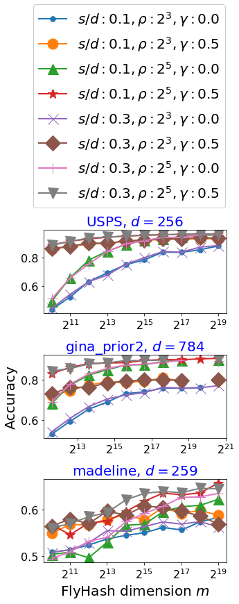
(a) FlyHash dimension $m$

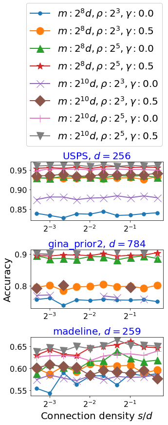
(b) Projection density $s/d$

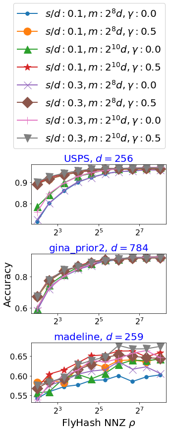
(c) FlyHash NNZ $\rho$

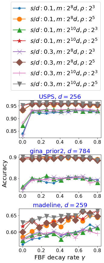
(d) FBF decay rate $\gamma$

Figure 4: FlyNN hyper-parameter dependence – Part I. Effect of the different FlyNN hyper-parameters $m$, $s$, $\rho$, $\gamma$ on FlyNN predictive performance for $3$ datasets – the horizontal axes correspond to the hyper-parameter being varied while fixing the remaining hyper-parameters. The vertical axes correspond to the 10-fold cross-validated accuracy for the given hyper-parameter configuration (higher is better). Note the log scale on the horizontal axes. Please view in color.

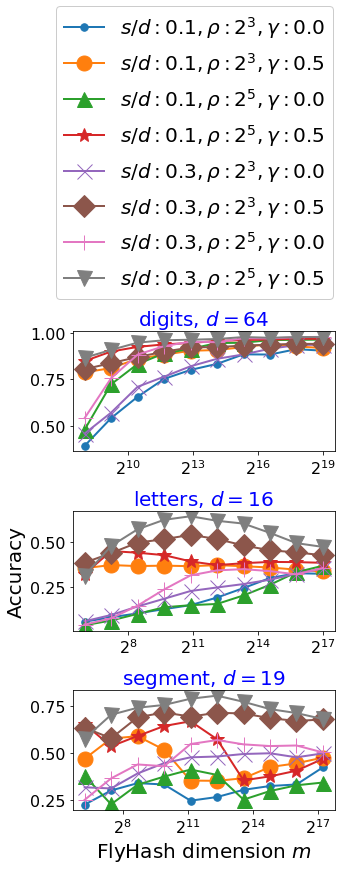
(a) FlyHash dimension $m$

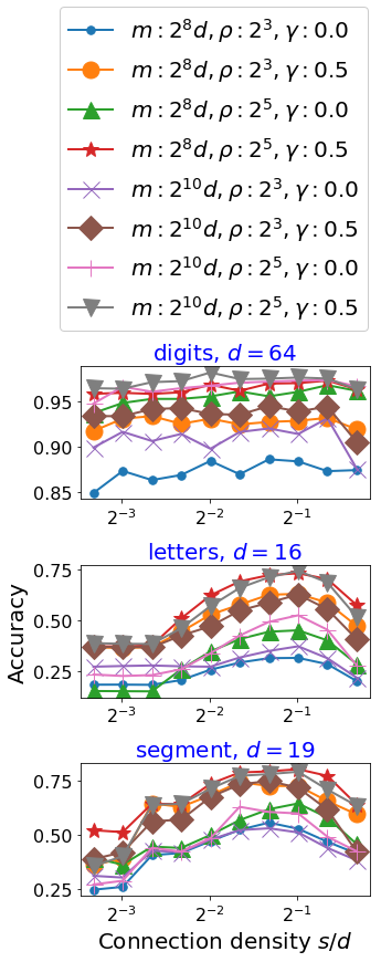
(b) Projection density $s/d$

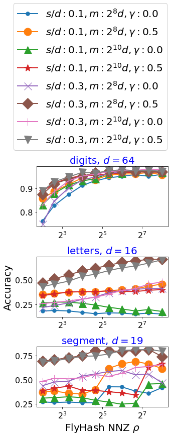
(c) FlyHash NNZ $\rho$

(d) FBF decay rate $\gamma$

Figure 5: FlyNN hyper-parameter dependence – Part II. Effect of the different FlyNN hyper-parameters $m$, $s$, $\rho$, $\gamma$ on FlyNN predictive performance for $3$ datasets – the horizontal axes correspond to the hyper-parameter being varied while fixing the remaining hyper-parameters. The vertical axes correspond to the 10-fold cross-validated accuracy for the given hyper-parameter configuration (higher is better). Note the log scale on the horizontal axes. Please view in color.

The results in Figures 4(a) & 5(a) indicate that, for fixed $\rho$ increasing $m$ improves the FlyNN accuracy, aligning with the theoretical guarantees, up until an upper bound. This behavior is clear for high dimensional datasets. This behavior is a bit more erratic for the lower dimensional sets. Larger values of $m$ improve performance, since it allows us to capture each class’ distribution with smaller random overlap between each class’ FBFs. But the theoretical guarantees also indicate that $\rho$ needs to be large enough, and if $m$ grows too large for any given $\rho$, the FlyNN accuracy might not improve any further.

Figures 4(b) & 5(b) indicate that for lower dimensional data (such as $d\leq 20$), increasing the projection density $s$ improves performance up to a point (around $s=0.5$), after which the performance starts degrading. This is probably because for smaller values of $s$, not enough information is captured by the sparse projection for small $d$; for large values of $s$, each row in the projection matrix $\mathsf{M}$ become similar to each other, hurting the similarity-preserving property of FlyHash. For higher dimensional datasets, the FlyNN performance appears to be somewhat agnostic to $s$ for any fixed $m$, $\rho$ and $\gamma$.

Figures 4(c) & 5(c) indicate that increase in $\rho$ leads to improvement in FlyNN performance since large values of $\rho$ better preserve pairwise similarities. However, if $\rho$ is too large relative to $m$, the sparsity of the subsequent per-class FBF go down, thereby leading to more overlap in the per-class FBFs. So $\rho$ needs to large as per the theoretical analysis, but not too large.

Figures 4(d) & 5(d) indicate that the FlyNN is somewhat agnostic to the FBF decay rate $\gamma$ for any value strictly greater than $0$ (corresponding to the binary FBF). But there is a significant drop in the FlyNN performance from $\gamma>0$ to $\gamma=0$ across all dataset – this behavior is fairly consistent and apparent.

D.7 Comparison to gradient descent based baseline

While we can compare nearest-neighbor-based methods (such as $k$NNC) to gradient-descent-based methods by comparing the best possible optimally tuned performances of each method, it is hard to do such a comparison with some form of parity in terms of computational or communication overhead. We attempt to draw one form of parity based on the communication overhead. Our first proposed scheme for FlyNNFL has a communication overhead of $O(m)$ where $m$ can be $O(n)$ is the most unfavorable setup. To this end, we wish to compare all schemes for an overall communication budget of $O(n)$. For stochastic gradient-descent based methods, involving communication in every gradient update on a batch of data per-party, a single epoch (a single pass of the data per-party) would correspond to $O(n)$ communication. This is also appropriate for another reason: all the training algorithms – TrainFlyNN (Algorithm 1), TrainFlyNNFLDP (Algorithm 2) – involve a single pass of the training data. Henceforth, we consider two baselines – logistic regression (LR) trained with a single epoch, and multi-layered perceptrons (MLPC) trained with a single epoch. To further remove confounding effects, and obtain the best-case performance for these gradient-descent-based schemes with a single epoch, we consider a centralized training for LR and MLPC instead of a true FL training; the performance of the centralized training usually provides an upperbound on the expected performance with FL training.

Hyper-parameter selection.

For LR, we consider logistic regression trained for a single epoch with a stochastic algorithm. We utilize the scikit-learn implementation (linear_model.LogisticRegression) and tune over the following hyper-parameters – (a) penalty type ($\ell_{1}$/$\ell_{2}$), (b) regularization $\in\left[2^{-10},2^{10}\right]$, (c) choice of solver (liblinear (Fan et al. 2008)/SAG (Schmidt, Le Roux, and Bach 2017)/SAGA (Defazio, Bach, and Lacoste-Julien 2014)), (d) with/without intercept, (e) one-vs-rest or multinomial for multi-class, (f) with/without class balancing (note that this class balancing operation makes this a two-pass algorithm since we need the first pass to weigh the classes appropriately). We consider a total of 960 hyper-parameter configurations for each of the 70 OpenML dataset. For MLPC, we consider a multi-layer perceptron trained for a single epoch with the “Adam” stochastic optimization scheme (Kingma and Ba 2014). We use sklearn.neural_network.MLPClassifier and tune over the following hyper-parameters – (a) number of hidden layers $\{1,2\}$, (b) number of nodes in each hidden layer $\{16,64,128\}$, (b) choice of activation function (ReLU/HyperTangent), (d) regularization, (e) batch size $\in\left[2,2^{8}\right]$, (f) initial learning rate $\in\left[10^{-5},0.1\right]$ (the rest of the hyper-parameters are left as scikit-learn defaults). This leads to a total of 720 hyper-parameters configurations for each of the 70 OpenML datasets.

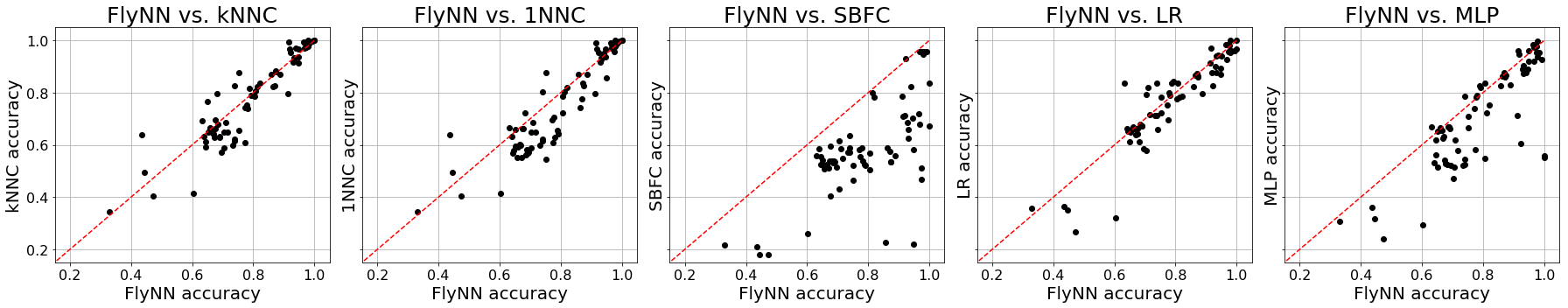
Figure 6: Performance of baselines relative to FlyNN on OpenML datasets. The scatter plots compare the best tuned FlyNN accuracy against that of $k$NNC, $1$NNC, SBFC, LR and MLPC with a point for each dataset, and the red dashed diagonal marking match to FlyNN accuracy.

Table 9: Comparing FlyNN to baselines on OpenML datasets with (i) Fraction of datasets FlyNN exceed baselines, (ii) Number of datasets on which FlyNN has wins(W)/ties(T)/losses(L) over baselines, (iii) Median improvement in normalized accuracy by FlyNN over baseline across all datasets, (iv) $p$-values for the paired two-sided t-test (TT), (v) $p$-values for the two-sided Wilcoxon signed rank test (WSRT).

Method	(i) Frac.	(ii) W/T/L	(iii) Imp.	(iv) TT	(v) WSRT
$k$NNC	0.55	39/2/30	0.35%	5.30E-2	7.63E-2
$1$NNC	0.66	47/2/22	2.36%	1.55E-5	2.81E-5
SBFC	0.99	70/0/1	25.4%	$<$1E-8	$<$1E-8
LR	0.62	44/1/26	1.80%	4.06E-2	7.68E-3
MLPC	0.75	53/0/18	6.17%	7.00E-8	1.00E-8

Results similar in form to the results in the main paper (Figure 1, Table 2) are presented in Figure 6 and Table 9. The results for $k$NNC, $1$NNC and SBFC are repeated for ease of comparison. FlyNN performs comparably to LR (with a single epoch), outperforming it on 62% of the datasets, and providing a 1.80% median improvement with $p$-values of 0.0406 (TT) and 0.00768 (WSRT), indicating significant difference. When compared to MLPC (with a single epoch), FlyNN has a much more favorable performance, outperforming on 75% of the datasets, and providing a 6.17% median improvement and $p$-values of the order of $10^{-8}$, indicating significant improvement. This highlights the ability of FlyNN to match or outperform gradient-descent-based methods (which are widely studied in the FL setting) when compared with some form of parity in the communication overhead across over 70 datasets from OpenML.

However, this comparison should be considered with the understanding that comparing inherently different machine learning methods can involve various caveats. In this comparison, we tried to explicitly discuss the choices we made and why we made them.

D.8 Empirical evaluation of Differentially Private FlyNNFL

To study the effect of $(\epsilon,0)$-differential privacy on the classification performance of FlyNNFL, we consider two sets of experiment. In one set of experiments, we consider the synthetic dataset (described in supplement §D.2), while in another, we consider the a binary classification version of the MNIST dataset, where we are trying to classify between the (hard-to-classify) digits 3 and 8.

Synthetic data.

In this set of experiments, we generate classification data in ${\mathbb{R}}^{d}$ with $d=30$ for a 2-class classification problem with 5 modes per class. We create two training datasets, one with $n=10^{4}$ samples and another with $n=10^{5}$ samples to study the effect of increasing the number of samples. To evaluate the performance, we utilize a heldout test set of size $10^{3}$ samples.

We consider 4 sets of hyper-parameters for FlyNN:

1. $m=300,s=3,\rho=15,\gamma=0.9$,

2. $m=300,s=3,\rho=30,\gamma=0.9$,

3. $m=600,s=3,\rho=15,\gamma=0.9$,

4. $m=600,s=3,\rho=30,\gamma=0.9$.

We consider a 2-party problem ($\tau=2$) where the training data is evenly between the parties, each with $\nicefrac{{n}}{{2}}$ samples. For each hyper-parameter, we first invoke TrainFlyNNFLDP with IS_DP = false and record the non-DP test error. Then, we invoke TrainFlyNNFLDP with DP enabled (that is IS_DP = true) with different values of $\epsilon\in[0.25,2.0]$ and $T\in[4,600]$. The test error for each pair of $(\epsilon,T)$ is noted – we perform 10 repetitions for each pair of $(\epsilon,T)$ and report the mean and the confidence interval of the obtained test error. The results are presented in Figure 7. The results in Figure 3(a) presents one of these results for $n=10^{5}$.

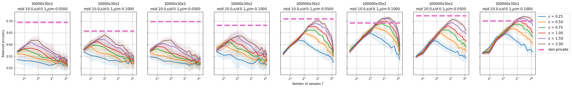
Figure 7: Effect of DP on the FlyNNFL accuracy for varying values of $\epsilon\in[0.25,2]$ and $T\in[4,600]$. The horizontal axis corresponds to the number of samples $T$ while the vertical axis corresponds to balanced classification accuracy (higher is better). In each of the plots, the horizontal dashed line corresponds to the accuracy of the non-private FlyNNFL (TrainFlyNNFLDP invoked with IS_DP = false). Each of the lines correspond to a particular value of $\epsilon$, and plots the mean accuracy over 10 repetitions with the confidence interval in the form of translucent ribbons around the lines. The 4 left plots correspond to the 4 FlyNN hyper-parameters with $n=10^{4}$ samples, while the 4 right plots correspond to the 4 FlyNN hyper-parameters with $n=10^{5}$ samples.

The results indicate the intuitive behaviour that, as the number of samples $T$ increases, the FlyNNFL performance improves up until a point and then it starts dropping. This behaviour is seen for all values of $\epsilon$ and all different hyper-parameters $(m,s,\rho,\gamma)$ of FlyNN. Comparing the 4 left plots (with $n=10^{4}$ samples) to the 4 right plots (with $n=10^{5}$ samples), we see that, with increasing number of points, the non-private test accuracy is not significantly affected, but the performance of the DP FlyNNFL improves significantly, and is able to almost match the non-private accuracy for all the FlyNN hyper-parameters for moderately high $\epsilon\in[1,2]$.

Figure 8 presents the dependence of the FlyNNFL accuracy on $\epsilon$ more explicitly. The experimental setup is the same as Figure 7, and, for each value of $\epsilon$, we select the $T$ with the best accuracy on the heldout set. We see the expected behaviour with the accuracy increasing with $\epsilon$. The results in Figure 3(b) presents one of these results for $n=10^{5}$.

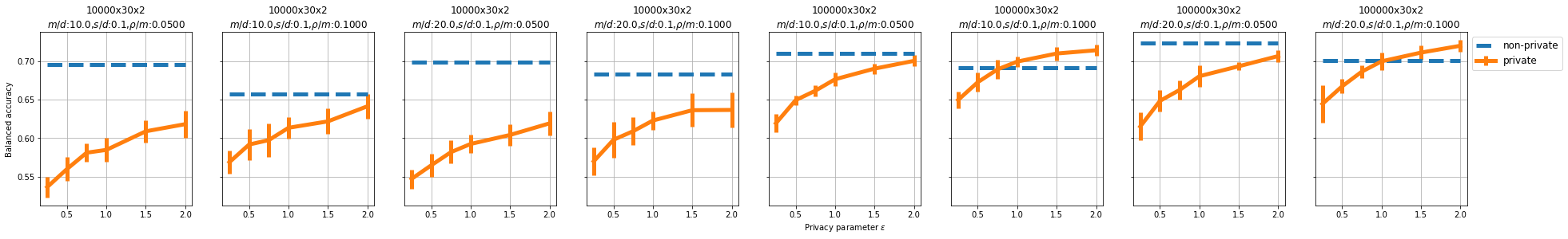
Figure 8: Effect of DP on the FlyNNFL accuracy for varying values of $\epsilon\in[0.25,2]$. The horizontal axis corresponds to the privacy level $\epsilon$, while the vertical axis corresponds to balanced classification accuracy (higher is better). In each of the plots, the blue horizontal dashed line corresponds to the accuracy of the non-private FlyNNFL (TrainFlyNNFLDP invoked with IS_DP = false). In each of the plots, the orange line corresponds to the best (over all values of $T$) mean $\pm$ standard deviation accuracy (aggregated over 10 repetitions) of the DP-enabled FlyNNFL with increasing $\epsilon$. The 4 left plots correspond to the 4 FlyNN hyper-parameters with $n=10^{4}$ samples, while the 4 right plots correspond to the 4 FlyNN hyper-parameters with $n=10^{5}$ samples.

MNIST 3 vs 8 binary classification.

We also evaluate the effect of DP on MNIST. For the binary 3 vs. 8 classification problem, $n\approx 12000$ and $d=784$. We select the following FlyNN hyper-parameters: $m/d=30,s/d=0.00625,\rho=0.1m,\gamma=0.9$. We perform a similar experiment as with synthetic data and compare the performance of non-private TrainFlyNNFLDP with 2 parties ($\tau=2$) to that of the DP-enabled TrainFlyNNFLDP with different values of $\epsilon\in[0.25,2]$ and $T\in[4,600]$. The results are presented in Figure 9. The results in Figure 9(a) presents the aforementioned trend where the accuracy of DP FlyNNFL improves with the number of samples $T$ up until a point at which it drops. Figure 9(b) presents the expected trend of the improving performance of DP FlyNNFL with increasing $\epsilon$.

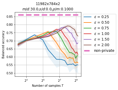
(a) $T$ vs accuracy for varying values of $\epsilon$.

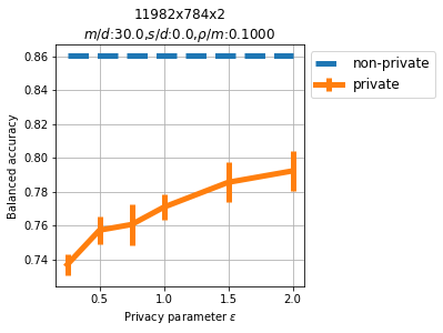
(b) $\epsilon$ vs accuracy

Figure 9: Effect of the FlyNNFL accuracy for varying values of $\epsilon\in[0.25,2]$ and $T\in[4,600]$ with MNIST dataset for a binary classification problem with labels $3$ and $8$. In figure 9(a), the horizontal axis corresponds to the number of samples $T$ while the vertical axis corresponds to balanced classification accuracy (higher is better); the horizontal dashed line corresponds to the accuracy of the non-private FlyNNFL (TrainFlyNNFLDP invoked with IS_DP = false), and each of the lines correspond to a particular value of $\epsilon$, and plots the mean accuracy over 10 repetitions with the confidence interval in the form of translucent ribbons around the lines. In figure 9(b), the horizontal axis corresponds to the privacy level $\epsilon$, while the vertical axis corresponds to balanced classification accuracy (higher is better); the blue horizontal dashed line corresponds to the accuracy of the non-private FlyNNFL (TrainFlyNNFLDP invoked with IS_DP = false), and the orange line corresponds to the best (over all values of $T$) mean $\pm$ standard deviation accuracy (aggregated over 10 repetitions) of the DP-enabled FlyNNFL with increasing $\epsilon$.

References

- Abadi et al. (2016) Abadi, M.; Barham, P.; Chen, J.; Chen, Z.; Davis, A.; Dean, J.; Devin, M.; Ghemawat, S.; Irving, G.; Isard, M.; et al. 2016. Tensorflow: A system for large-scale machine learning. In 12th USENIX symposium on operating systems design and implementation (OSDI 16), 265–283.
- Anchalia and Roy (2014) Anchalia, P. P.; and Roy, K. 2014. The k-nearest neighbor algorithm using Mapreduce paradigm. In International Conference on Intelligent Systems, Modeling and Simulation.
- Charikar (2002) Charikar, M. S. 2002. Similarity estimation techniques from rounding algorithms. In Proceedings of the thiry-fourth annual ACM symposium on Theory of computing, 380–388.
- Chaudhuri and Dasgupta (2014) Chaudhuri, K.; and Dasgupta, S. 2014. Rate of convergence of nearest neighbor classification. In Advances in Neural Information Processing Systems.
- Chen et al. (2020) Chen, H.; Chilotti, I.; Dong, Y.; Poburinnaya, O.; Razenshteyn, I.; and Riazi, M. S. 2020. Scaling up secure approximate k-nearest neighbor search. In USENIX security symposium.
- Cover and Hart (1967) Cover, T.; and Hart, P. 1967. Nearest neighbor pattern classification. IEEE Transactions on Information Theory, 13: 21–27.
- Dasgupta et al. (2018) Dasgupta, S.; Sheehan, T. C.; Stevens, C. F.; and Navlakha, S. 2018. A neural data structure for novelty detection. Proceedings of the National Academy of Sciences, 115(51): 13093–13098.
- Dasgupta, Stevens, and Navlakha (2017) Dasgupta, S.; Stevens, C. F.; and Navlakha, S. 2017. A neural algorithm for a fundamental computing problem. Science, 358(6364): 793–796.
- Defazio, Bach, and Lacoste-Julien (2014) Defazio, A.; Bach, F.; and Lacoste-Julien, S. 2014. SAGA: A fast incremental gradient method with support for non-strongly convex composite objectives. In Advances in neural information processing systems, 1646–1654.
- Devroye et al. (1994) Devroye, L.; Gyorfi, L.; Krzyzak, A.; and Lugosi, G. 1994. On the strong universal consistency of nearest neighbor regression function estimates. The annals of Statistics, 22: 1371–1385.
- Fan et al. (2008) Fan, R.-E.; Chang, K.-W.; Hsieh, C.-J.; Wang, X.-R.; and Lin, C.-J. 2008. LIBLINEAR: A library for large linear classification. Journal of machine learning research, 9(Aug): 1871–1874.
- Fix and Hodges (1951) Fix, E.; and Hodges, J. L. 1951. Discriminatory analysis-nonparametric discrimination: consistency properties. Tech. Rep. California Univ. Berkeley.
- Gonzalez-Lopez, Ventura, and Cano (2018) Gonzalez-Lopez, J.; Ventura, S.; and Cano, A. 2018. Distributed nearest neighbor classification for large-scale multi-label data on spark. Future Generation Computer Systems, 87: 66–82.
- Gottlieb, Kontorovich, and Nisnevitch (2014) Gottlieb, L.-A.; Kontorovich, A.; and Nisnevitch, P. 2014. Near-optimal sample compression for nearest neighbors. In Advances in Neural Information Processing Systems.
- Guyon (2003) Guyon, I. 2003. Design of experiments of the NIPS 2003 variable selection benchmark. In NIPS 2003 workshop on feature extraction and feature selection.
- Hinton et al. (2012) Hinton, G. E.; Srivastava, N.; Krizhevsky, A.; Sutskever, I.; and Salakhutdinov, R. R. 2012. Improving neural networks by preventing co-adaptation of feature detectors. arXiv preprint arXiv:1207.0580.
- Kairouz and McMahan (2021) Kairouz, P.; and McMahan, H. B. 2021. Advances and Open Problems in Federated Learning. Foundations and Trends® in Machine Learning, 14(1): –.
- Kavukcuoglu et al. (2010) Kavukcuoglu, K.; Sermanet, P.; Boureau, Y.-L.; Gregor, K.; Mathieu, M.; and LeCun, Y. 2010. Learning convolutional feature hierarchies for visual recognition. In Advances in neural information processing systems, 1090–1098.
- Keivani, Sinha, and Ram (2017) Keivani, O.; Sinha, K.; and Ram, P. 2017. Improved maximum inner product search with better theoretical guarantees. In 2017 International Joint Conference on Neural Networks (IJCNN), 2927–2934. IEEE.
- Keivani, Sinha, and Ram (2018) Keivani, O.; Sinha, K.; and Ram, P. 2018. Improved maximum inner product search with better theoretical guarantee using randomized partition trees. Machine Learning, 107(6): 1069–1094.
- Kingma and Ba (2014) Kingma, D. P.; and Ba, J. 2014. Adam: A method for stochastic optimization. arXiv preprint arXiv:1412.6980.
- Koenigstein, Ram, and Shavitt (2012) Koenigstein, N.; Ram, P.; and Shavitt, Y. 2012. Efficient retrieval of recommendations in a matrix factorization framework. In Proceedings of the 21st ACM international conference on Information and knowledge management, 535–544.
- Krizhevsky, Hinton et al. (2009) Krizhevsky, A.; Hinton, G.; et al. 2009. Learning multiple layers of features from tiny images.
- Krizhevsky, Sutskever, and Hinton (2012) Krizhevsky, A.; Sutskever, I.; and Hinton, G. E. 2012. Imagenet classification with deep convolutional neural networks. In Advances in neural information processing systems, 1097–1105.
- Larochelle and Hinton (2010) Larochelle, H.; and Hinton, G. E. 2010. Learning to combine foveal glimpses with a third-order Boltzmann machine. In Advances in neural information processing systems, 1243–1251.
- Lecun (1995) Lecun, Y. 1995. The MNIST database of handwritten digits.
- Lecun and Bengio (1995) Lecun, Y.; and Bengio, Y. 1995. Convolutional Networks for Images, Speech and Time Series, 255–258. The MIT Press.
- Li et al. (2020) Li, T.; Sahu, A. K.; Talwarkar, A.; and Smith, V. 2020. Federated learning: Challenges, methods and future directions. IEEE Signal Processing Magazine, 37(3): 50–60.
- Liang et al. (2021) Liang, Y.; Ryali, C. K.; Hoover, B.; Grinberg, L.; Navlakha, S.; Zaki, M. J.; and Krotov, D. 2021. Can a Fruit Fly Learn Word Embeddings? arXiv preprint arXiv:2101.06887.
- Mallio, Triguero, and Herrera (2015) Mallio, J.; Triguero, I.; and Herrera, F. 2015. A mapreduce-based k-nearest neighbor approach for big data classification. In IEEE Trustcom/BigDataSE/ISPA.
- McMahan et al. (2017) McMahan, H. B.; Moore, E.; Ramage, D.; Hampson, S.; and Arcas, B. A. 2017. Communication efficient learning of deep neural networks from decentralized data. In International Conference on Artificial Intelligence and Statistics.
- Mnih et al. (2014) Mnih, V.; Heess, N.; Graves, A.; et al. 2014. Recurrent models of visual attention. In Advances in neural information processing systems, 2204–2212.
- Pedregosa et al. (2011) Pedregosa, F.; Varoquaux, G.; Gramfort, A.; Michel, V.; Thirion, B.; Grisel, O.; Blondel, M.; Prettenhofer, P.; Weiss, R.; Dubourg, V.; et al. 2011. Scikit-learn: Machine learning in Python. Journal of machine learning research, 12(Oct): 2825–2830.
- Qi and Atallah (2008) Qi, Y.; and Atallah, M. J. 2008. Efficient privacy-preserving k-nearest neighbor search. In International Conference on Distributed Computing Systems.
- Qiao, Duan, and Cheng (2019) Qiao, X.; Duan, J.; and Cheng, G. 2019. Rate of convergence of large scale nearest neighbor classification. In Advances in Neural Information Processing Systems.
- Ram and Gray (2012) Ram, P.; and Gray, A. G. 2012. Maximum inner-product search using cone trees. In Proceedings of the 18th ACM SIGKDD International Conference on Knowledge Discovery and Data Mining, 931–939.
- Ram and Sinha (2021) Ram, P.; and Sinha, K. 2021. FlyNN: Fruit-fly Inspired Federated Nearest Neighbor Classification. International Workshop on Federated Learning for User Privacy and Data Confidentiality in Conjunction with ICML 2021 (FL-ICML’21).
- Ryali et al. (2020) Ryali, C. K.; Hopfield, J. J.; Grinberg, L.; and Krotov, D. 2020. Bio-Inspired Hashing for Unsupervised Similarity Search. arXiv preprint arXiv:2001.04907.
- Schmidt, Le Roux, and Bach (2017) Schmidt, M.; Le Roux, N.; and Bach, F. 2017. Minimizing finite sums with the stochastic average gradient. Mathematical Programming, 162(1-2): 83–112.
- Schoppmann et al. (2020) Schoppmann, P.; Vogelsang, L.; Gascón, A.; and Balle, B. 2020. Secure and Scalable Document Similarity on Distributed Databases: Differential Privacy to the Rescue. Proceedings on Privacy Enhancing Technologies, 2020(2): 209–229.
- Shaul, Feldman, and Rus (2018) Shaul, H.; Feldman, D.; and Rus, D. 2018. Secure -ish Nearest Neighbors Classifier. arXiv preprint arXiv:1801.07301.
- Shaul, Feldman, and Rus (2020) Shaul, H.; Feldman, D.; and Rus, D. 2020. Secure k-ish nearest neighbor classifier. Proceedings on Privacy Enhancing Technologies, 2020(3): 42–61.
- Sinha and Ram (2021) Sinha, K.; and Ram, P. 2021. Fruit-fly Inspired Neighborhood Encoding for Classification. In Proceedings of the 27th ACM SIGKDD Conference on Knowledge Discovery & Data Mining, 1470–1480.
- Van Rijn et al. (2013) Van Rijn, J. N.; Bischl, B.; Torgo, L.; Gao, B.; Umaashankar, V.; Fischer, S.; Winter, P.; Wiswedel, B.; Berthold, M. R.; and Vanschoren, J. 2013. OpenML: A collaborative science platform. In Joint european conference on machine learning and knowledge discovery in databases, 645–649. Springer.
- Wu et al. (2019) Wu, W.; Parampalli, U.; Liu, J.; and Xian, M. 2019. Privacy Preserving K-Nearest Neighbor Classification over Encrypted Database in Outsourced Cloud Environments. World Wide Web, 22(1): 101–123.
- Xiao, Rasul, and Vollgraf (2017) Xiao, H.; Rasul, K.; and Vollgraf, R. 2017. Fashion-mnist: a novel image dataset for benchmarking machine learning algorithms. arXiv preprint arXiv:1708.07747.
- Xiong, Chitti, and Liu (2006) Xiong, L.; Chitti, S.; and Liu, L. 2006. K nearest neighbor classification across multiple private databases. In International Conference on Information and Knowledge Management.
- Zhan, Chang, and Matwin (2008) Zhan, J. Z.; Chang, L.; and Matwin, S. 2008. Privacy preserving k-nearest neighbor classification. ACM Transactions on Intelligent Systems and Technology, 1(1): 46–51.
- Zhang et al. (2020) Zhang, W.; Chen, X.; Liu, Y.; and Xi, Q. 2020. A distributed storage and computation k-nearest neighbor algorithm based cloud-edge computing for cyber physical systems. IEEE Access, 8: 50118–50130.