GEO-BLEU: Similarity Measure for Geospatial Sequences

Abstract.

In recent geospatial research, the importance of modeling large-scale human mobility data and predicting trajectories is rising, in parallel with progress in text generation using large-scale corpora in natural language processing. Whereas there are already plenty of feasible approaches applicable to geospatial sequence modeling itself, there seems to be room to improve with regard to evaluation, specifically about measuring the similarity between generated and reference trajectories. In this work, we propose a novel similarity measure, GEO-BLEU, which can be especially useful in the context of geospatial sequence modeling and generation. As the name suggests, this work is based on BLEU, one of the most popular measures used in machine translation research, while introducing spatial proximity to the idea of $n$-gram. We compare this measure with an established baseline, dynamic time warping, applying it to actual generated geospatial sequences. Using crowdsourced annotated data on the similarity between geospatial sequences collected from over 12,000 cases, we quantitatively and qualitatively show the proposed method’s superiority.

1. Introduction

Geospatial sequence modeling over human mobility trajectories and language modeling in natural language processing (NLP) can be seen analogously, regarding places as words and human mobility trajectories as sentences. On the geospatial side, the main workhorse is next place prediction (NPP) (Schreckenberger et al., 2018) in which a model predicts the place a person moves to at the next time step on the basis of the past trajectory and other features, and repeating NPP while reusing predicted places as context directly leads to geospatial sequence generation. Also, this approach can naturally extend to sequence-to-sequence or translation, assuming a model generates a trajectory using another corresponding trajectory, e.g., one in a past period, as context. The importance of this kind of self-supervised approach is surging in geospatial research, and many modeling methods known in NLP and other related fields are feasibly applicable to geospatial problem settings. Meanwhile, the area of evaluation still seems to be needing further consideration.

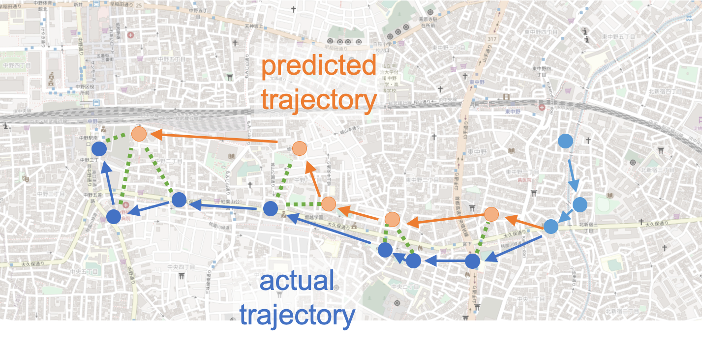
Figure 1. Predicted and actual human mobility trajectories in a relatively short time period, e.g. tens of minutes.

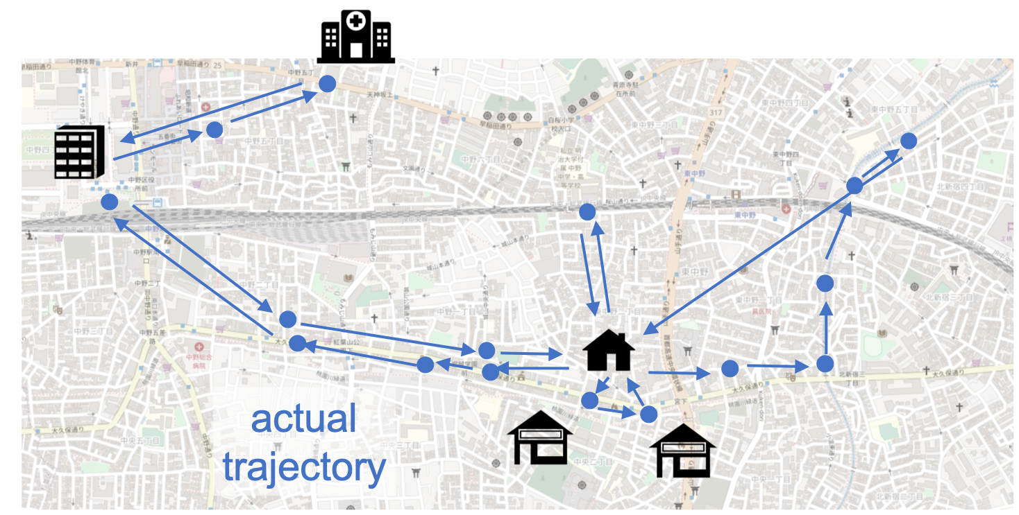
Figure 2. A complex human mobility trajectory in a relatively long time period, e.g. several days.

• Dynamic time warping (DTW) (Vintsyuk, 1968; Sakoe and Chiba, 1978) has long been known as a way to evaluate the distance of two given sequences, and it has been used in geospatial research as well as in many other fields. An essential characteristic of DTW is that it aligns the sequences for measuring entirely, without considering local features shared between them. It is suitable to treat entirely aligned sequences, but not so when treating involved sequences for which step-by-step alignment does not make much sense.

• BLEU (Papineni et al., 2002) is one of the most popular measures for similarity used in NLP, especially in machine translation. BLEU uses local features of given sequences, word $n$-grams, and is suitable to treat not completely aligned sequences. Regarding places in sequences as words and their contiguous combinations as geospatial $n$-grams, we can apply this to evaluate the similarity of geospatial trajectories on the basis of local features. However, it has another disadvantage; the geospatial $n$-grams need to be exactly the same to be counted as “matched”, and very close but slightly displaced ones do not contribute to the outcome. In other words, spatial proximity, which is potentially an important property for similarity, is not taken into account when using BLEU.

There can actually be situations where DTW is not suitable. Figure 1 shows predicted and actual trajectories in a relatively short time period, e.g. tens of minutes. In this case, trajectories are simple enough to be aligned in a meaningful way as illustrated by the dotted green lines, and thus DTW is applicable here without problems. On the other hand, when the time period of prediction is relatively long, e.g. several days, trajectories to be predicted will become more involved as illustrated in Figure 2. The trajectory is not a straight line from one place to another anymore but a combination of subtrajectories such as one from home to the office, one from the office to a nearby hospital, and so on. In this problem setting, we can expect that a predicted trajectory shares some motifs or subtrajectories with the actual one locally but not that the whole predicted and actual trajectories can be aligned from the start to the end in a meaningful way, possibly having subtrajectories occurring in a different order.

In this work, we propose a novel alternative, GEO-BLEU, extending BLEU to incorporate the idea of geospatial proximity into its core concept while utilizing local features and not requiring alignment. To evaluate the measure’s performance, we use a translation problem of human mobility trajectories as a plausible test case for similarity and distance measures; we collected trajectories consisting of smartphone locations and modeled them in a sequence-to-sequence manner. The modeling task is to predict peoples’ daily trajectories under the self-restraint of COVID-19 on the basis of trajectories in the pre-COVID-19 period, which ultimately leads to understanding behavioral implications of COVID-19 and contributing to the field of urban dynamics. At the same time, we focus on the similarity measure in this work and stay away from stepping into this COVID-19-specific research question. We apply our proposed measure, GEO-BLEU, and other two baselines, BLEU and DTW, to sequences generated by this translation model, comparing generated sequences and actual sequences. After that, we compare these scores with crowdsourced annotated data to quantify how consistent the measures and human intuition are, showing the proposed method’s superiority.

2. Existing and Proposed Measures

In this section, we first explain DTW and BLEU and then describe our proposed measure GEO-BLEU. Also, using a toy problem, we demonstrate a notable characteristic of the proposed method.

2.1. Existing Measures

2.1.1. Dynamic Time Warping.

Dynamic time warping (DTW) (Vintsyuk, 1968; Sakoe and Chiba, 1978) is a distance-like measure for comparing the similarity between two sequences which was first developed in speech recognition but then has been used in various fields including geospatial research. The method involves finding the optimal alignment between two sequences $X=(x_{1},x_{2},\ldots,x_{M})$ and $Y=(y_{1},y_{2},\ldots,y_{N})$. One possible way of alignment is represented as a sequence of pairs between elements in $X$ and those in $Y$: $P=((x_{i_{1}},y_{j_{1}}),(x_{i_{2}},y_{j_{2}}),\ldots,(x_{i_{l}},y_{j_{l}}),\\ \ldots,(x_{i_{L}},y_{j_{L}}))$ where $i_{l}\in[1:M],j_{l}\in[1:N]$ and $L=\max(M,N)$. Also, there are three conditions for $P$ to be valid alignment:

• the boundary condition $(i_{1},j_{1})=(1,1)$ and $(i_{L},j_{L})=(M,N)$, which requires the start of $X$ and $Y$ and the end of them must be matched respectively,

• monotonicity condition $i_{l}\leq i_{l+1}$ and $j_{l}\leq j_{l+1}$ for $l\in[1:L-1]$, which preserves the time-ordering of elements, and

• step size condition $(i_{l+1}-i_{l},j_{l+1}-j_{l})\in\{(1,1),(1,0),(0,1)\}$.

The cost for such an alignment $P$ is calculated as the sum of the pairwise distance $d(x_{i_{l}},y_{j_{l}})$:

(1) $$cost(P)=\sum\limits_{l=1}^{L}d(x_{i_{l}},y_{j_{l}})$$

where $d(\cdot,\cdot)$ is usually the Euclidean distance between two places. Using this, we can represent DTW as the minimum cost given by the optimal $P$:

(2) $$DTW=\min_{P}cost(P).$$

As for the actual procedure of optimization, we followed a technical report (Senin, 2008).

2.1.2. BLEU

BLEU (Papineni et al., 2002) is a measure being heavily used for evaluating machine translation systems for quantifying how close generated candidates are to reference human translations. BLEU uses word $n$-grams as the unit of comparison and considers the ratio of $n$-grams matched between the generated and reference sentences to all the $n$-grams in the generated candidates for a given $n$. The ratio, which is called modified precision $p_{n}$, is obtained as follows

(3) $$p_{n}=\frac{\sum\limits_{S\in C}\;\sum\limits_{n\text{-}gram\in S}\text{Count}_{\text{matched}}(n\text{-}gram)}{\sum\limits_{S\in C}\;\sum\limits_{n\text{-}gram^{\prime}\in S}\text{Count}(n\text{-}gram^{\prime})}$$

where $C$ is the candidate corpus, and $S$ is each of the candidate sentences in it. Actually, $p_{n}$ tends to become large when the candidates are too short. To correct this unintended effect, BLEU uses a factor called the brevity penalty $BP$, which is given by

(4) $$BP=\begin{cases}1,&\text{if $c>r$}\\ e^{1-r/c},&\text{if $c\leq r$}\end{cases}$$

where $c$ is the sum of the candidates’ lengths, and $r$ is that of the references. Taking the weighted geometric average of the modified precision scores for $n\in\{1,\ldots,N\}$ while applying $BP$, resultant BLEU score $B$ is defined as

(5) $$BLEU=BP\cdot\exp\bigg{(}\sum\limits_{n=1}^{N}w_{n}\log p_{n}\bigg{)}$$

where $w_{n}$ is the positive weight summing up to 1. The original work of BLEU uses $N=4$ and $w_{n}=\frac{1}{N}$ for $n\in\{1,\ldots,4\}$, and we follow the settings in the current study. It should be noted that BLEU is for evaluating candidate and reference sentences of the whole corpus and not for evaluating a single candidate sentence. Nevertheless, we borrow the approach of BLEU to devise a measure applicable to a single pair of sentences which can be an alternative to DTW.

2.2. GEO-BLEU

Our proposed measure GEO-BLEU is based on BLEU but intended to be an alternative to DTW, which means it measures a distance or similarity of a given pair of sequences. At the same time, it borrows the concept of $n$-gram from NLP, relaxing the matching condition so that the score reflects the proximity of a given pair of $n$-grams.

As the first step, we introduce the geospatial revision of $n$-gram as a chunk of locations $(q_{1},\ldots,q_{n})$ where each location $q_{k}$ is represented as a point in two-dimensional space. In addition, we define the similarity score $s$ of a pair of $n$-grams $g_{v}=(v_{1},\ldots,v_{n})$ and $g_{w}=(w_{1},\ldots,w_{n})$ on the basis of proximity as follows

(6) $$s(g_{v},g_{w})=\prod_{k=1}^{n}\exp(-\beta\,d(v_{k},w_{k}))$$

where $d(\cdot,\cdot)$ is the Euclidean distance between two locations, and $\beta$ is a coefficient for adjusting the scale. In this manner, the similarity between $n$-grams is evaluated to become one when two $n$-grams are exactly matched. Also, the far two $n$-grams go away, the closer the value asymptotically comes to zero.

Next, we consider the way to match $n$-grams in the candidate sequence and those in reference. In BLEU, the matching is conducted by the function $Count_{\text{matched}}(n\text{-}gram)$ in Equation 3; it gives one if the same $n$-gram remains “unused” in the reference sentences, eliminating that “used” $n$-gram instance from the pool for subsequent matching, and otherwise gives zero. For GEO-BLEU, which incorporates the concept of proximity, we let an $n$-gram on the candidate side form a pair with the closest unused $n$-gram remaining on the reference side, prohibiting $n$-grams on the reference side from being reused as in the BLEU’s original matching rule. We greedily optimize the set of such pairs so that the sum of the similarity scores comes close to the maximum value. Denoting the optimized set of pairs as $P=\{(g_{c_{1}},g_{r_{1}}),\ldots,(g_{c_{L}},g_{r_{L}})\}$ where $L$ is the shorter of the candidate’s and reference’s lengths, $g_{c_{k}}$ is an $n$-gram of the candidate sequence, and $g_{r_{k}}$ is that of the reference sequence, we define our $n$-gram-based similarity $q_{n}$ for a pair of a candidate sequence $S$ and its reference sequence as

(7) $$q_{n}=\frac{\sum\limits_{(g_{c},g_{r})\in P}s(g_{c},g_{r})}{\sum\limits_{n\text{-}gram\in S}Count(n\text{-}gram)}$$

which can be computed as shown in Algorithm 1. Taking the weighted geometric mean for a range of $n$ in the same manner as Equation 5 and introducing the brevity penalty $BP$ as in Equation 4, the proposed similarity measure GEO-BLEU is given as

(8) $$GEO\text{-}BLEU=BP\cdot\exp\bigg{(}\sum\limits_{n=1}^{N}w_{n}\log q_{n}\bigg{)}.$$

In our experiments, we use $\beta=1$, $N=3$, and $w_{n}=\frac{1}{N}$ for $n\in\{1,2,3\}$.

If BLEU is applied to evaluating a single candidate, there can be cases in which the modified precision becomes zero. On the contrary, the modified-precision equivalent of GEO-BLEU always has a non-zero value due to the relaxed matching, and this property makes GEO-BLEU more feasible and suitable for evaluating a single candidate sequence.

Algorithm 1 Computation of Equation 7 including greedy matching of $n$-grams in candidate and reference sequences

1:Input: two arrays of $n$-grams, candidate $C=\{{g_{c}}_{1},\ldots,{g_{c}}_{L_{c}}\}$ and reference $R=\{{g_{r}}_{1},\ldots,{g_{r}}_{L_{r}}\}$

2:$similaritySum\leftarrow 0$

3:Create array $A$, initially empty

4:for all $g_{c},g_{r}\in C\times R$ do

5:     $similarity\leftarrow s(g_{c},g_{r})$ using Equation 6

6:     Append tuple $(g_{c},g_{r},similarity)$ to $A$

7:end for

8:Sort $A$ by $similarity$ in decreasing order

9:while $A$ is not empty do

10:     $g_{c},g_{r},similarity\leftarrow A[0]$

11:     $similaritySum\leftarrow similaritySum+similarity$

12:     Remove all the tuples involving $g_{c}$ or $g_{r}$ from $A$

13:end while

14:return $similaritySum/L_{c}$

2.2.1. Characteristics of GEO-BLEU

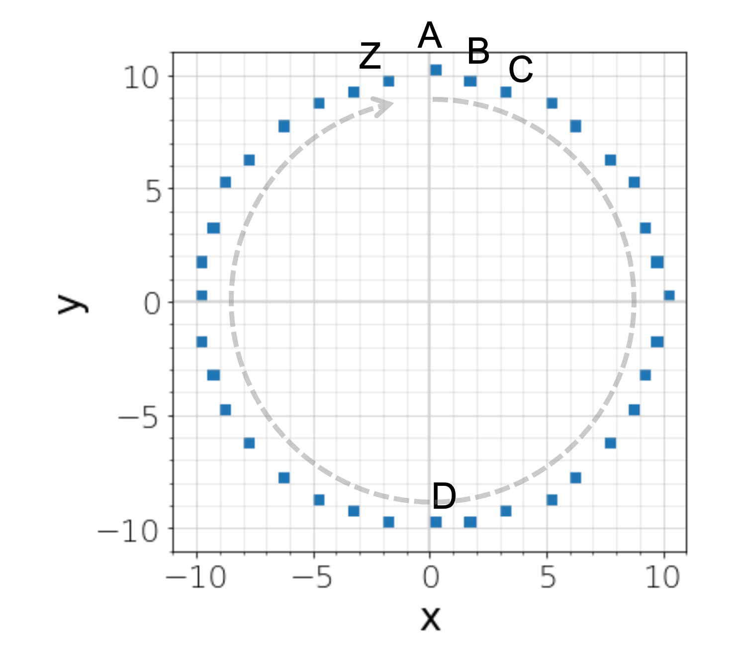
Figure 3. A sample sequence consisting of 36 grid cells placed over a circle of 10 km radius.

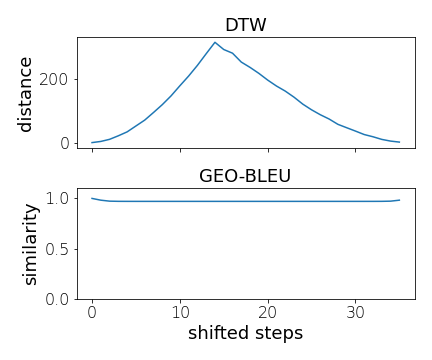
Figure 4. The scores of DTW and GEO-BLEU depending on the extent of the phase shift between the original and its shifted, derived sequence.

To illustrate the characteristics of GEO-BLEU and its difference from DTW, we apply the two measures to simple toy sequences in two-dimensional space and compare the results. As shown in Figure 3, we consider 36 grid cells with sides of 0.5 km placed over a circle of 10 km radius at almost regular intervals. Our original sample sequence starts from cell A, goes clockwise through B, C, and the following, and ends at Z as shown as the dashed arc arrow. Then, by moving the start and end points clockwise and one step at a time, i.e., by shifting the phase forward, we can generate variations such as one going clockwise from B to A, another from C to B, and so on for evaluating the similarity with or distance from the original. Here, it is crucial that whether they are similar or different depends on the evaluations’ purpose and point of view, and there is no definite criterion in that regard. Considering the original sequence and another with the opposite phase starting from D, they are completely different when aligned wholly. In this view, the distance between the first cells of the sequences is 20 km, the maximum possible number in this setting, and it does not change in the following aligned pairs, such as one between the second cells of the two sequences. On the other hand, those two sequences can be seen as almost identical when concerned with the local features, as they share almost all the cells and chunks except for those around the start and end. Among these conflicting points of view, GEO-BLEU is for comparing sequences on the basis of local features as in the latter example, while DTW views two sequences wholly aligned as in the former.

Figure 4 shows the actual distance calculated by DTW and similarity by GEO-BLEU between the original and shifted sequences where the $x$-axis denotes the number of the shifted steps. The subject of comparison is the original sequence itself at $x=0$, two sequences have the opposite phases at around $x=18$, and the phase difference becomes very small again at the rightmost point $x=35$. The results are contrasting; the value of DTW is significantly changing depending on $x$, while that of GEO-BLEU is staying around the maximum possible value as two sequences are always similar considering their local features. As illustrated, GEO-BLEU is a measure for comparing sequences on the basis of their partial or local features and without aligning them wholly.

3. Experiments

3.1. Human Mobility Trajectory Dataset

For this study, a web service company, Yahoo! JAPAN, provided us with smartphone GPS records of their users, which had originally been collected for their services. The users have agreed to provide their location information for research purposes, and the data are anonymized so that individuals cannot be identified and that personal properties such as gender and age are unknown. Each GPS record consists of a user’s ID, timestamp, longitude, and latitude.

One thing to note here is that the trajectory data is inherently noisy to some extent from various reasons such as the error of GPS sensors and timing for sending the location data which is adjusted by the user’s situation and smartphone’s conditions. Thus, it is not guaranteed that two identical actual trajectories turn into the identical sequences in the obtained data.

Using this smartphone GPS data, we extracted records from two consecutive periods, one from Oct. 1st, 2019 to Mar. 31st, 2020 and the other from Apr. 1st to May 25th in 2020. The periods were determined so that the data captures two different modes of the society in Japan, one mode without the influence of COVID-19, which corresponds to the former period, and the other mode under nationwide self-restraint of activities to prevent the spread of the infection, which corresponds to the latter period. As for deciding the specific dates, we referred to dates of the government’s relevant announcements in addition to public stringency index data (Ritchie et al., 2020).

From this set of GPS records, we prepared one million pairs of trajectories representing how the mobility pattern of a person in the pre-COVID-19 period has changed in the mid-COVID-19 period. In this data preparation process, the longitudes and latitudes in the GPS records are aggregated and discretized into 500m-square grid cells on an hourly basis so that a sequence of grid cells corresponds to a trajectory of a person. Using this set of GPS records, we obtained 1 million pairs of sequences as follows:

• aggregated the longitudes and latitudes so that it represents a trajectory of the person, keep trajectories spreading over both periods and discard the rest

• summarized and discretized the longitudes and latitudes into 500m-square grid cells representing hourly positions, and

• took out the longest partial sequence which is contained within the Tokyo metropolitan area for each of two periods of a pair so that the sequence does not contain unknown places.

Then, we allocated 10,000 pairs to the validation set, another 10,000 pairs to the test set, and the rest to the training set. The resultant vocabulary size, i.e. the number of unique 500m-square cells within the area appearing in the sequences, is 10,584. Also, The average length of sequences is 90.5 in the former period and 124.5 in the latter period. Considering that each step stands for an hourly position, each of these sequences usually amounts to a mobility pattern spanning over several days rather than a short trajectory within a day.

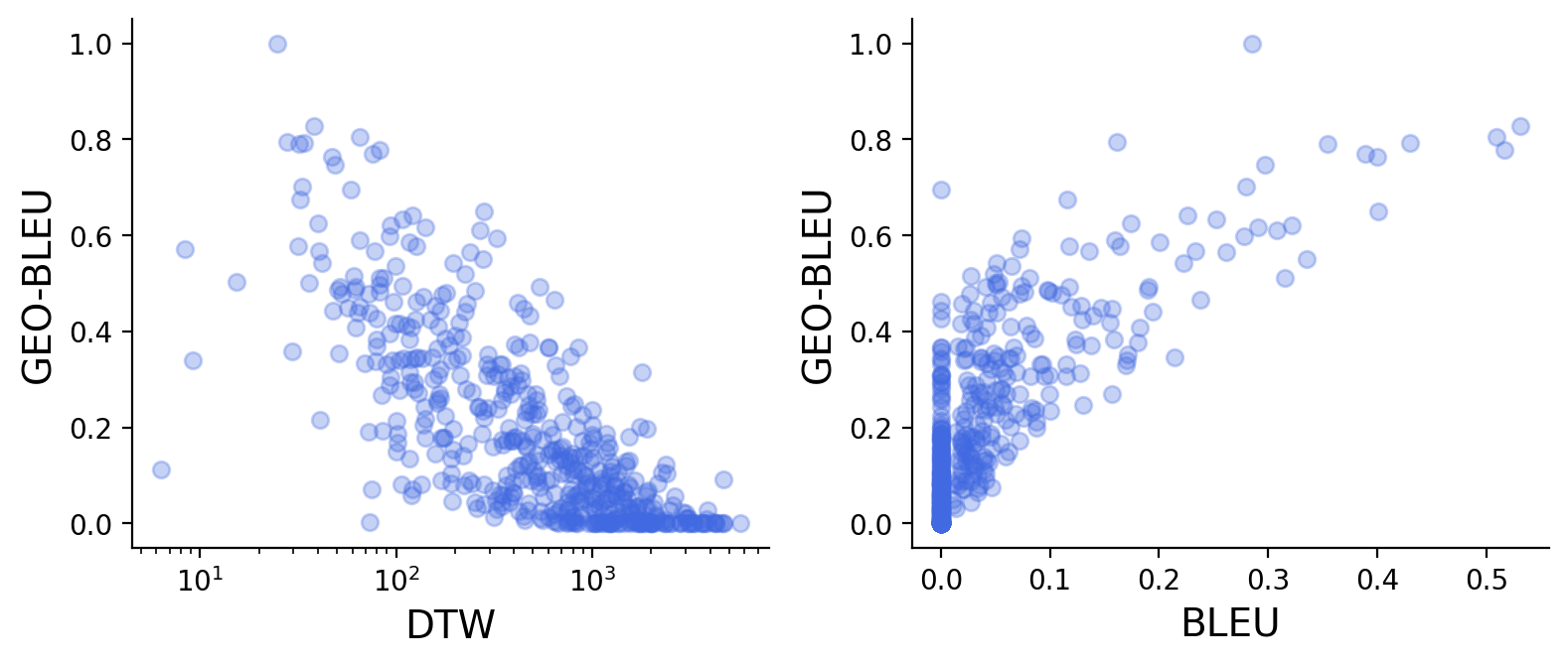
Figure 5. Comparison of GEO-BLEU scores with DTW and BLEU scores, respectively, for the 500 pairs of generated and actual human mobility trajectories.

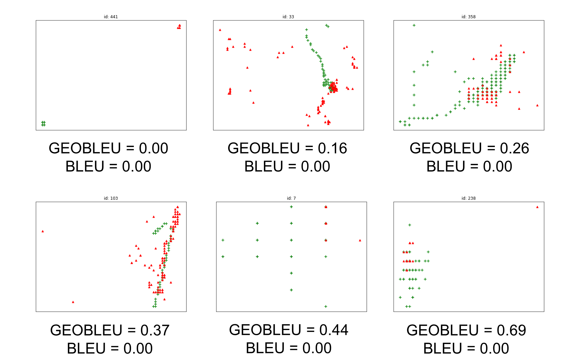
Figure 6. Examples of trajectory pairs where the BLEU scores are 0, but GEO-BLEU scores are non-zero (except for the top left one). GEO-BLEU is capable of capturing subtle differences and similarities compared to BLEU.

3.2. Model and Training

We trained a seq2seq model (Sutskever et al., 2014; Cho et al., 2014) consisting of a pair of two-layer LSTM-RNNs using the dataset for ten epochs so that it can generate a person’s trajectory in the mid-COVID-19 period given a trajectory in the pre-COVID-19 period. After the training finished, we took out a model with the lowest validation loss and applied it to sample sequence generation as in the next section.

3.3. Evaluation and Results

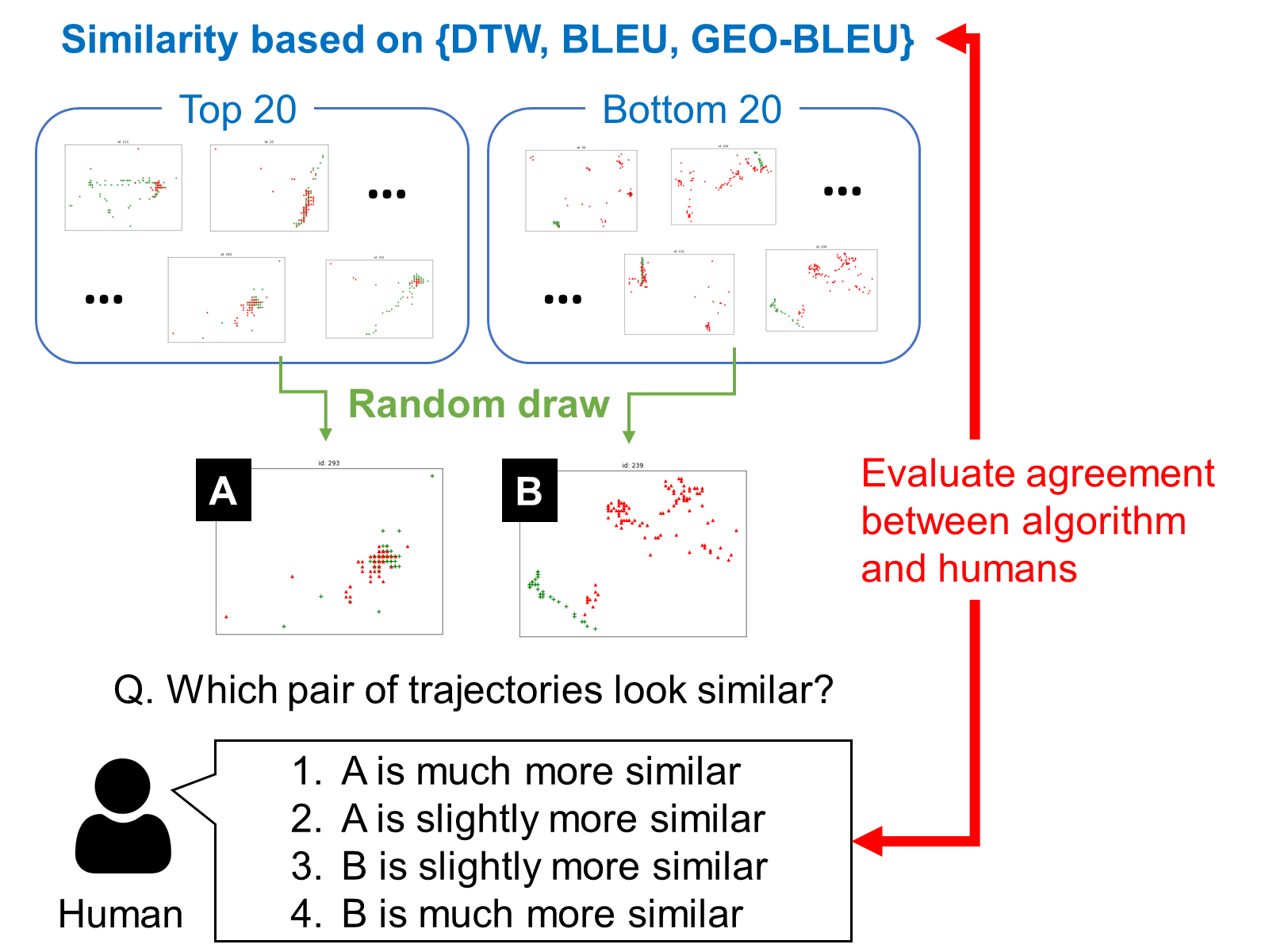
Figure 7. Outline of crowdsourcing framework used to validate the performance of GEO-BLEU.

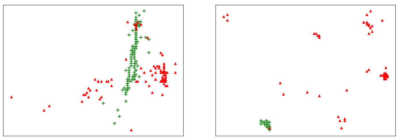
Figure 8. An example of annotation cases for evaluating each measure. The red dots show the steps of a generated trajectory, and the green dots show the steps of its corresponding actual trajectory. In this example, the left side actually belongs to the top-20 pairs and the right side the bottom-20 pairs, and the annotator is asked to distinguish which side comes from the top-20. The easier the cases of a measure are, the better the measure is considered to be.

Table 1. The average of annotation scores for each measure.

Method	normalized DTW	BLEU	GEO-BLEU
Score	0.550	0.530	0.699

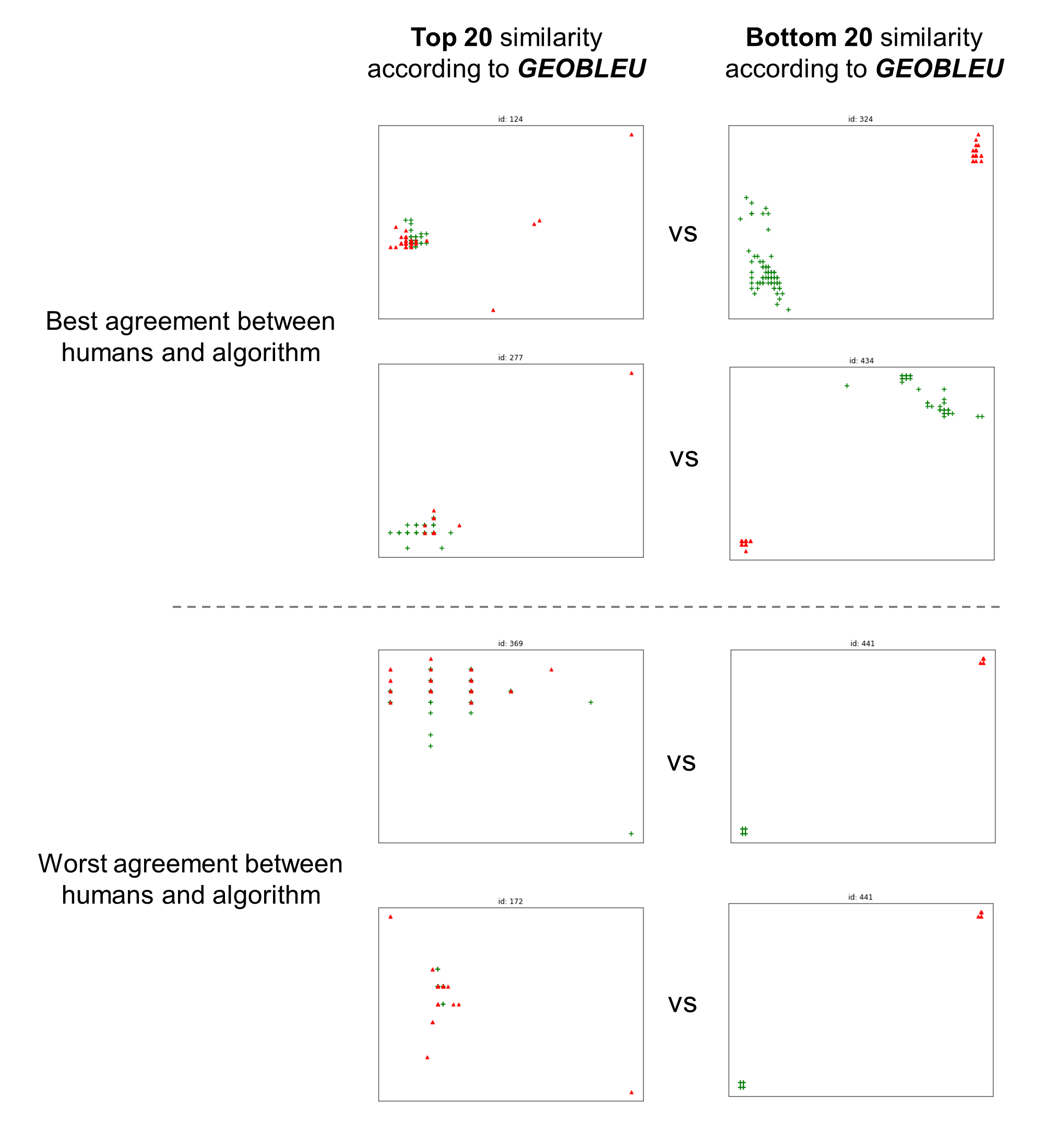
Figure 9. Comparison of cases with the most frequent agreements and disagreements between the humans and GEO-BLEU scores.

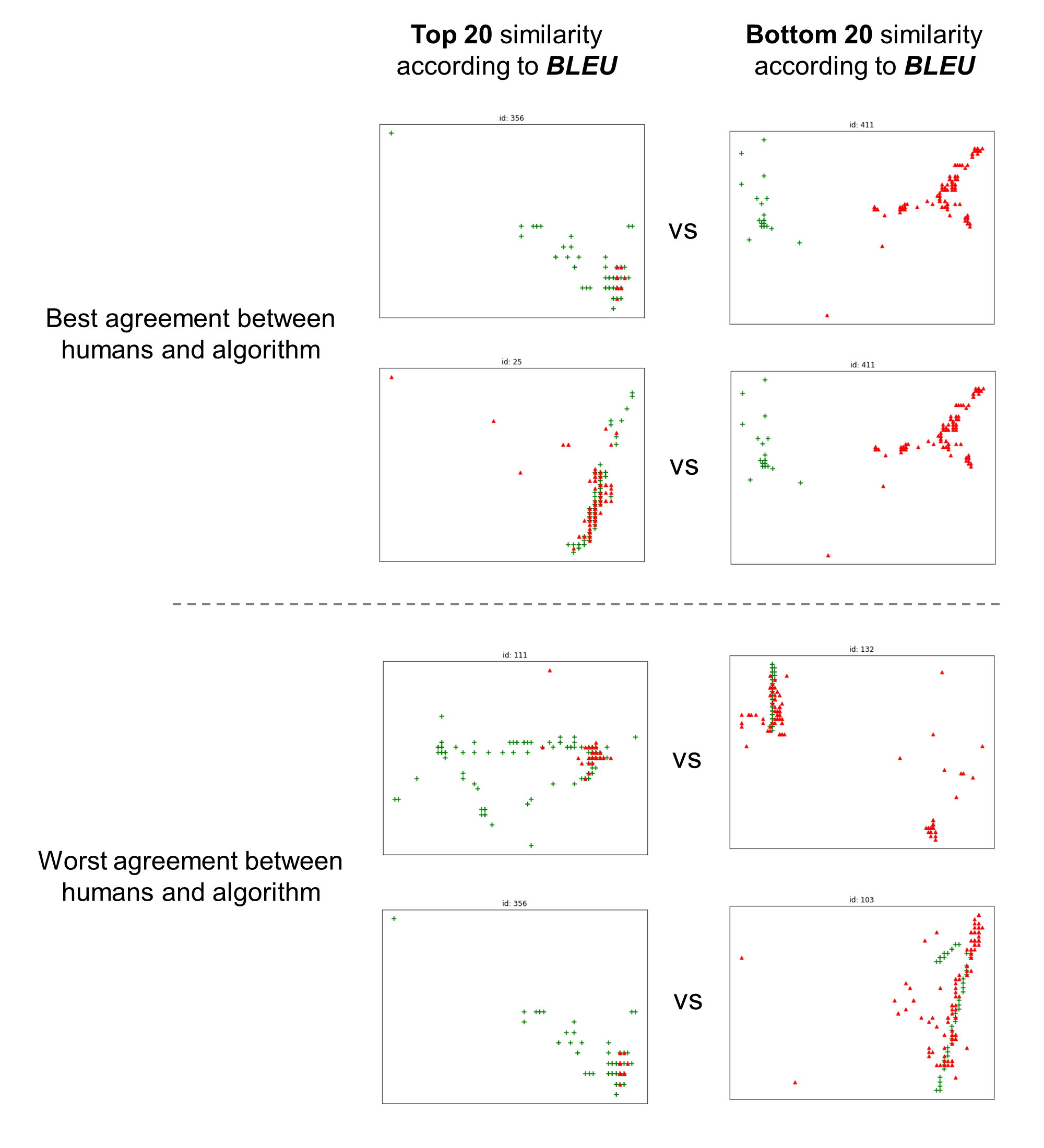
Figure 10. Comparison of cases with the most frequent agreements and disagreements between the humans and scores.

We generated 500 sample sequences using the trained model and the test set. Then, we scored each sequence with three measures, normalized DTW, GEO-BLEU, and BLEU, comparing the generated trajectory with the actual one in the dataset. As DTW has a dependency on the sequence length as in Equation 1, we normalize the raw scores dividing them by $L$. Actually, BLEU is a quality measure not of a single sentence but of the entire corpus. However, we dared to apply BLEU for evaluating each sequence here for reference, treating a pair of sequences as a small corpus, to show the difference between the original BLEU and GEO-BLEU. Figure 5 shows the DTW, GEO-BLEU, and BLEU scores for each of the samples in the dataset. We observe a negative correlation between DTW and GEO-BLEU and a positive correlation between BLEU and GEO-BLEU, which is intuitive. Comparing BLEU to GEO-BLEU, we see that GEO-BLEU is able to assign positive scores to instances where the BLEU score is zero, since GEO-BLEU is designed to capture the subtle differences (where BLEU assigns a zero score even for small distance differences). Figure 6 shows some examples where BLEU gave a score of zero, however GEO-BLEU gave some positive scores, ranging from 0 to 0.69. We can see here how GEO-BLEU gives partial credit for having some overlap or closeness in the predicted data over the ground truth data.

3.4. Crowdsourced Experiment

To evaluate how convincing the scores given by a measure are, we sorted the 500 pairs of generated and actual trajectories by each of three measures into descending order of similarity, obtaining three lists of the same entries but in different orders. Then, we took out the top-20 pairs and the bottom-20 pairs from those lists. There are $20\times 20=400$ possible combinations between the top pairs and bottom pairs for each measure, and for each such combination, we asked annotators which pair of generated and actual sequences look more similar, showing the top and bottom pairs side-by-side, as shown in Figure 8. An annotation is given as one of four options: the left is clearly similar, the left is somewhat similar, the right is somewhat similar, and the right is clearly similar. We assign a positive score to a case if the judgment is consistent with the measure: 1.0 if the top-side is judged as clearly similar and 0.5 if it is somewhat similar. If the judgment is inconsistent with the measure, the score becomes -1.0 for “clearly similar” and -0.5 for “somewhat similar” to give a penalty. We presented one case to ten different annotators and collected $400\times 10\times 3=12,000$ judgments. The overall procedure of the crowdsourced experiment is shown in Figure 7. Table 1 shows the averaged score for three measures, and GEO-BLEU is superior to normalized DTW in this comparison. While the purpose of BLEU is not a single-sequence measurement as in this evaluation, the scores themselves imply that GEO-BLEU derived from it is modified so that it becomes more suitable to the current problem settings.

Figures 9 and 10 show examples where the labels given by humans and the algorithms (GEO-BLEU and BLEU, respectively) had the largest and least agreement. The top two rows of Figure 9 show two example pairs where both the algorithm (GEO-BLEU) and humans indicated that the trajectories on the left are much more similar than the one on the right. The lower two rows of Figure 9 are examples where humans indicated that the trajectory pairs on the right hand side were more similar compared to the ones on the left, which is not intuitive. We suspect that human labelers mistook the meaning of ‘similarity of two trajectories’ in these cases.

4. Related Work

Many studies have proposed methods to measure the similarity of two movement trajectories. First, there are two major types of cases: one is to compare and evaluate the entire movement trajectory, and the other is to compare and evaluate a part of the movement trajectory. The former is called complete match measure and the latter is called partial match measure, as summarized in the following section. Other types of measures have already been proposed as described in a survey (Su et al., 2020). Still, to the best of our knowledge, this work is the first to apply the concept of “geospatial $n$-gram” to such evaluation, to take into account the local features of sequences.

4.1. Complete Match Measure

Complete match measure is a method of comparing two movement trajectories with respect to all measurement points. For example, if the two movement trajectories are perfectly matched, the distance between them is zero. However, in many cases, there are differences between the two movement trajectories, and the amount of those differences is compared. The difficulty with this method of comparing movement trajectories is that it must take into account not only distance but also time differences. In addition, the length of the movement trajectory changes on a case-by-case basis. For instance, if trajectory A is 10 km in 2 hours and trajectory B is 130 km in 8 hours, it is difficult to simply compare the two trajectories.

The most basic method for a complete match is the Euclidean distance (Sanderson and Wong, 1980; Takens, 1980), which calculates the difference in the norm of the trajectories to be compared. It was first proposed as a distance measure between time series and was once considered as one of the most widely used distance functions since the 1960s (Faloutsos et al., 1994; Priestley, 1980). It is now also used to evaluate movement trajectories. In this case, the trajectories must have the same length.

The most famous algorithm for complete match is Dynamic Time Warping (DTW) (Bhadane and Shah, 2017; Cai et al., 2018). This method has been used for a long time to measure distances in time series data (Chan et al., 2003; Salvador and Chan, 2007; Yi et al., 1998; Pietroszek et al., 2017), and it is now also used to compare movement trajectories. The algorithm is simple (Myers et al., 1980), and the lengths of the two trajectories do not have to be the same.

4.2. Partial Match Measure

Partial match measure is a method to measure similarity in only one part of two movement trajectories with a large amount of information. Two well-known methods for partial match are the Longest common subsequence (LCSS) and edit distance on real sequence (EDR) methods.

First, LCSS measures (Ichiye and Karplus, 1991; Robinson, 1990) the length of the sequence common to two trajectories at successive points. For example, two people who were separated at the start meet at a certain point, travel the same distance for a while, and then break up again. In this case, the LCSS method does not consider the degree of separation between the two trajectories, but focuses only on the common trajectory, and the longer the trajectory, the more similar the trajectories are.

EDR (Panagiotakis et al., 2009; Lee et al., 2007) is a method to calculate how much processing of the movement trajectory A should be done to match the movement trajectory B. For example, the similarity is defined as the cost of repeatedly performing insertions, deletions, or substitutions until the two match. The greater the processing cost, the lower the similarity between the two movement trajectories. Many proposals have been made regarding the definition of processing methods and costs.

Methods such as LCSS and EDR, which measure similarity only for a part of the movement trajectory, are often effective as distance measures without being complicated to process. However, the goal of this research is to measure similarity as perceived by humans. People often make judgments of similarity by looking at the entire image, and partial match is not appropriate for this purpose.

5. Conclusion

We proposed a novel similarity measure of sequences, GEO-BLEU, extending BLEU by incorporating proximity into the core concept and using place $n$-grams as local features so that it can evaluate the similarity of predicted and reference trajectories without aligning them step by step from the start to the end.

The effectiveness and characteristics of GEO-BLEU was tested on two types of data sets: a set of artificial data and an in-the-wild data set based on actual user movement trajectories. In a realistic setting about self-supervised geospatial sequence modeling, GEO-BLEU is more consistent with annotators’ intuition for similarity than an existing popular measure, DTW. The proposed GEO-BLEU should be applicable to many future studies in diverse research fields as a practical evaluation index for similarity of spatial trajectories in general.

References

- (1)
- Bhadane and Shah (2017) Chetashri Bhadane and Ketan Shah. 2017. Analysis of User Similarity Measures Using GPS Trajectories. In 2017 International Conference on Computing, Communication, Control and Automation (ICCUBEA). IEEE, 1–6.
- Cai et al. (2018) Qiqin Cai, Lyuchao Liao, Fumin Zou, Subin Song, Jierui Liu, and Meirun Zhang. 2018. Trajectory similarity measuring with grid-based DTW. In International Conference on Smart Vehicular Technology, Transportation, Communication and Applications. Springer, 63–72.
- Chan et al. (2003) F.K.-P. Chan, A.W.-C. Fu, and C. Yu. 2003. Haar wavelets for efficient similarity search of time-series: with and without time warping. IEEE Transactions on Knowledge and Data Engineering 15, 3 (2003), 686–705. https://doi.org/10.1109/TKDE.2003.1198399
- Cho et al. (2014) Kyunghyun Cho, Bart van Merriënboer, Caglar Gulcehre, Dzmitry Bahdanau, Fethi Bougares, Holger Schwenk, and Yoshua Bengio. 2014. Learning Phrase Representations using RNN Encoder–Decoder for Statistical Machine Translation. In Proceedings of the 2014 Conference on Empirical Methods in Natural Language Processing (EMNLP). Association for Computational Linguistics, Doha, Qatar, 1724–1734. https://doi.org/10.3115/v1/D14-1179
- Faloutsos et al. (1994) Christos Faloutsos, M. Ranganathan, and Yannis Manolopoulos. 1994. Fast Subsequence Matching in Time-Series Databases. In Proceedings of the 1994 ACM SIGMOD International Conference on Management of Data (Minneapolis, Minnesota, USA) (SIGMOD ’94). Association for Computing Machinery, New York, NY, USA, 419–429. https://doi.org/10.1145/191839.191925
- Ichiye and Karplus (1991) Toshiko Ichiye and Martin Karplus. 1991. Collective motions in proteins: A covariance analysis of atomic fluctuations in molecular dynamics and normal mode simulations. Proteins: Structure, Function, and Bioinformatics 11, 3 (1991), 205–217. https://doi.org/10.1002/prot.340110305 arXiv:https://onlinelibrary.wiley.com/doi/pdf/10.1002/prot.340110305
- Lee et al. (2007) Jae-Gil Lee, Jiawei Han, and Kyu-Young Whang. 2007. Trajectory Clustering: A Partition-and-Group Framework. In Proceedings of the 2007 ACM SIGMOD International Conference on Management of Data (Beijing, China) (SIGMOD ’07). Association for Computing Machinery, New York, NY, USA, 593–604. https://doi.org/10.1145/1247480.1247546
- Myers et al. (1980) C. Myers, L. Rabiner, and A. Rosenberg. 1980. Performance tradeoffs in dynamic time warping algorithms for isolated word recognition. IEEE Transactions on Acoustics, Speech, and Signal Processing 28, 6 (1980), 623–635. https://doi.org/10.1109/TASSP.1980.1163491
- Panagiotakis et al. (2009) Costas Panagiotakis, Nikos Pelekis, and Ioannis Kopanakis. 2009. Trajectory Voting and Classification Based on Spatiotemporal Similarity in Moving Object Databases. In Advances in Intelligent Data Analysis VIII, Niall M. Adams, Céline Robardet, Arno Siebes, and Jean-François Boulicaut (Eds.). Springer Berlin Heidelberg, Berlin, Heidelberg, 131–142.
- Papineni et al. (2002) Kishore Papineni, Salim Roukos, Todd Ward, and Wei-Jing Zhu. 2002. BLEU: A Method for Automatic Evaluation of Machine Translation. In Proceedings of the 40th Annual Meeting on Association for Computational Linguistics (Philadelphia, Pennsylvania) (ACL ’02). Association for Computational Linguistics, USA, 311–318. https://doi.org/10.3115/1073083.1073135
- Pietroszek et al. (2017) Krzysztof Pietroszek, Phuc Pham, and Christian Eckhardt. 2017. CS-DTW: Real-Time Matching of Multivariate Spatial Input against Thousands of Templates Using Compute Shader DTW. In Proceedings of the 5th Symposium on Spatial User Interaction (Brighton, United Kingdom) (SUI ’17). Association for Computing Machinery, New York, NY, USA, 159. https://doi.org/10.1145/3131277.3134355
- Priestley (1980) M. B. Priestley. 1980. STATE-DEPENDENT MODELS: A GENERAL APPROACH TO NON-LINEAR TIME SERIES ANALYSIS. Journal of Time Series Analysis 1, 1 (1980), 47–71. https://doi.org/10.1111/j.1467-9892.1980.tb00300.x arXiv:https://onlinelibrary.wiley.com/doi/pdf/10.1111/j.1467-9892.1980.tb00300.x
- Ritchie et al. (2020) Hannah Ritchie, Edouard Mathieu, Lucas Rodés-Guirao, Cameron Appel, Charlie Giattino, Esteban Ortiz-Ospina, Joe Hasell, Bobbie Macdonald, Diana Beltekian, and Max Roser. 2020. Coronavirus Pandemic (COVID-19). Our World in Data (2020). Retrieved from: https://ourworldindata.org/coronavirus.
- Robinson (1990) Mark T. Robinson. 1990. The temporal development of collision cascades in the binary-collision approximation. Nuclear Instruments and Methods in Physics Research Section B: Beam Interactions with Materials and Atoms 48, 1 (1990), 408–413. https://doi.org/10.1016/0168-583X(90)90150-S
- Sakoe and Chiba (1978) H. Sakoe and S. Chiba. 1978. Dynamic programming algorithm optimization for spoken word recognition. IEEE Transactions on Acoustics, Speech, and Signal Processing 26, 1 (1978), 43–49. https://doi.org/10.1109/TASSP.1978.1163055
- Salvador and Chan (2007) Stan Salvador and Philip Chan. 2007. Toward Accurate Dynamic Time Warping in Linear Time and Space. Intell. Data Anal. 11, 5 (oct 2007), 561–580.
- Sanderson and Wong (1980) Arthur C. Sanderson and Andrew K. C. Wong. 1980. Pattern Trajectory Analysis of Nonstationary Multivariate Data. IEEE Transactions on Systems, Man, and Cybernetics 10, 7 (1980), 384–392. https://doi.org/10.1109/TSMC.1980.4308519
- Schreckenberger et al. (2018) Christian Schreckenberger, Simon Beckmann, and Christian Bartelt. 2018. Next Place Prediction: A Systematic Literature Review. In Proceedings of the 2nd ACM SIGSPATIAL Workshop on Prediction of Human Mobility (Seattle, WA, USA) (PredictGIS 2018). Association for Computing Machinery, New York, NY, USA, 37–45. https://doi.org/10.1145/3283590.3283596
- Senin (2008) Pavel Senin. 2008. Dynamic Time Warping Algorithm Review. Technical Report. University of Hawaii at Manoa.
- Su et al. (2020) Han Su, Shuncheng Liu, Bolong Zheng, Xiaofang Zhou, and Kai Zheng. 2020. A survey of trajectory distance measures and performance evaluation. The VLDB Journal 29, 1 (2020), 3–32.
- Sutskever et al. (2014) Ilya Sutskever, Oriol Vinyals, and Quoc V. Le. 2014. Sequence to Sequence Learning with Neural Networks. In Proceedings of the 27th International Conference on Neural Information Processing Systems - Volume 2 (Montreal, Canada) (NIPS’14). MIT Press, Cambridge, MA, USA, 3104–3112.
- Takens (1980) Floris Takens. 1980. Motion under the influence of a strong constraining force. In Global Theory of Dynamical Systems, Zbigniew Nitecki and Clark Robinson (Eds.). Springer Berlin Heidelberg, Berlin, Heidelberg, 425–445.
- Vintsyuk (1968) T. K. Vintsyuk. 1968. Speech discrimination by dynamic programming. Cybernetics 4 (1968), 52–57. https://doi.org/10.1007/BF01074755
- Yi et al. (1998) Byoung-Kee Yi, H.V. Jagadish, and C. Faloutsos. 1998. Efficient retrieval of similar time sequences under time warping. In Proceedings 14th International Conference on Data Engineering. 201–208. https://doi.org/10.1109/ICDE.1998.655778