VPVnet: a velocity-pressure-vorticity neural network method for the Stokes’ equations under reduced regularity

Abstract

We present VPVnet, a deep neural network method for the Stokes’ equations under reduced regularity. Different with recently proposed deep learning methods [40, 51] which are based on the original form of PDEs, VPVnet uses the least square functional of the first-order velocity-pressure-vorticity (VPV) formulation ([30]) as loss functions. As such, only first-order derivative is required in the loss functions, hence the method is applicable to a much larger class of problems, e.g. problems with non-smooth solutions. Despite that several methods have been proposed recently to reduce the regularity requirement by transforming the original problem into a corresponding variational form, while for the Stokes’ equations, the choice of approximating spaces for the velocity and the pressure has to satisfy the LBB condition additionally. Here by making use of the VPV formulation, lower regularity requirement is achieved with no need for considering the LBB condition. Convergence and error estimates have been established for the proposed method. It is worth emphasizing that the VPVnet method is divergence-free and pressure-robust, while classical inf-sup stable mixed finite elements for the Stokes’ equations are not pressure-robust. Various numerical experiments including 2D and 3D lid-driven cavity test cases are conducted to demonstrate its efficiency and accuracy.

76D07, 76M25, 65N12, 65N15, 35B45.

1 Stokes’ equations

Recently, the deep neural network (DNN) methods have attracted remarkable attention in the field of computational fluid dynamics [9, 33, 57, 61]. In contrast to classical methods such as finite element, finite difference, and finite volume, the DNN approach does not require a mesh topology and can achieve good accuracy even when the domain of interest is presented by scattered discrete points [50]. Moreover, it requires less number of parameters to achieve the same accuracy as with finite element method on the grid points[37]. And it can lessen or even overcome the curse of dimensionality for high-dimensional problems [20], it also has great potential in nonlinear approximations [51, 55]. However, the performance of existing DNN methods may degrade for the Navier-Stokes equations with low regularity, e.g. when sharp local gradients present in a broad computational domain [48, 39]. Noting that most DNN methods such as the recently developed physics informed neural network (PINN) method [33] employs the residual of equations as the loss function, which requires derivatives of variables that is only applicable to problems whose solutions are sufficiently smooth, for example $(\bm{u},p)$ at least in $[H^{2}(\Omega)]^{2}\times H^{1}(\Omega)$ for the Stokes equations, and is not able to cope properly with problems that have nonsmooth solutions. As exactly solving the Stokes’s equations with low regularity is the preliminary for many Navier-Stokes applications such as the lid driven cavity problems and other problems with singular sources and sharp interfaces [2, 15, 30], etc. In this paper, we propose a deep neural network method for the Stokes’ equations with reduced regularity, i.e. $(\bm{u},p)\in[H^{1}(\Omega)]^{2}\times H^{1}(\Omega)$.

For simplicity, consider the following Stokes’ problem which seeks a velocity field $\bm{u}$ and a pressure unknown $p$ satisfying

$$\left\{\begin{split}-\nu\Delta\bm{u}+\nabla p&=\bm{f},\qquad{\rm in}\ \Omega,\\ \nabla\cdot\bm{u}&=0,\qquad{\rm in}\ \Omega,\\ \bm{u}&=\bm{g},\qquad{\rm on}\ \Gamma,\\ \end{split}\right.$$ (1)

where $\Omega$ is a bounded polygonal domain with boundary $\Gamma=\partial\Omega$ in $d$ ($d=2$ or $3$) dimension, $\nu>0$ is a constant viscosity parameter, $\bm{f}=(f^{(1)},\cdots,f^{(d)})$ represents external source, $\bm{g}$ is a given Dirichlet boundary condition, and the pressure $p$ is assumed to have mean value zero; i.e., $\int_{\Omega}pd\Omega=0$. Noting that the classical solution of (1) satisfies $\bm{u}\in[C^{2}(\Omega)\cap C^{0}(\Omega)]^{d}$ and $p\in C^{1}(\Omega)$.

Various deep learning based methods have been proposed and explored recently for the simulation of partial differential equations, such as the least square methods [17, 10], the deep Ritz methods [19], the physics-informed neural network (PINN) methods [51, 52, 33] and the variational formulation based methods [34, 35] among many others [11, 42, 28, 29, 55]. Here we roughly classify these methods according to their formulation of the loss functions; the reader is referred to [4, 35] and the references therein for a more detailed review. The least square methods may trace back to the 1990s., Dissanayake and Phan-Thhien [17] have proposed training neural networks via a least square functional that based on the original formulation of the PDEs. Thereafter the method have been further developed and it has been shown that the sampling points can be obtained by a random sampling [26], which is beneficial for high dimensional problems. Despite these advantages, for a second-order PDE, the minimization of the loss function over admissible functions leads to a fourth-order PDE, which is a more difficult problem than the original one [10]. Moreover, the method is only applicable to problems whose solutions are sufficiently smooth, more precisely, at least in $H^{2}(\Omega)$. Several methods have been recently proposed by transforming the original PDEs to the corresponding weak form so as to lower the regularity requirement. For example, the deep Ritz method [19] uses the energy functional of the underlying PDEs as loss functions, hence only first-order spatial derivatives is required for the second-order elliptic PDEs. However, the method only applies to problems that have a underlying minimization principle. In addition to that, variational type neural network methods [34, 35] have been proposed. These methods train the neural network by minimizing variational residuals of PDEs over a set of test functions with their compact supports located at different regions in space and time. The loss function is expected to be discretization free and highly parallelizable [35] and the methods also employ lower order derivatives. For instance, numerical experiments have shown good performance of the variational type methods for advection-diffusion problems with high Peclet numbers.

As for the Stokes problems, which is the main concern of this paper, different deep learning methods based on the least square functional of the original PDEs have been proposed and verified in [40, 11, 51]. As mentioned previously, these methods are only applicable to problems whose solutions are sufficiently smooth, for $(\bm{u},p)$ at least in $[H^{2}(\Omega)]^{2}\times H^{1}(\Omega)$. Since the Stokes’ problem does not have an underlying minimization principle, methods such as the deep Ritz method do not apply. As for the variational type methods, it is well known that the variational formulation of the Stokes’ problem leads to a saddle-point problem. Consequently, the combination of velocity and pressure interpolations is required to satisfy the famous Ladyzhenskaya-Babu$\check{s}$ka-Brezzi (LBB) condition [22, 41]. On the other side, by using different activation functions such as Sigmoid, deep neural network can give rise to a very wide range of functional classes that can be drastically different from the piecewise polynomial function classes used in classical finite element methods. These function classes, however, do not usually form a linear vector space [64] which makes it tricky to apply the variational type neural network methods to Stokes’ equations.

In this paper, we propose a neural network method that is based on the first-order velocity-pressure-vorticity (VPV) system [30, 31, 32], namely VPVnet, to approximate the solution of the Stokes’ equations. The least square functional of the VPV system leads to a minimization problem rather than a saddle point problem, thus the combination of velocity, vorticity and pressure interpolations is not subject to the restriction of the LBB conditions. And no artificial boundary conditions need to be devised for the vorticity. Moreover, the VPV least square functional only requires first-order spatial derivatives, hence it has less regularity requirements on the solutions and is applicable to a much larger class of problems compared with least square methods that based on the original form of the Stokes’ equations. Note that similar ideas of making use of first order systems has also been used for the second-order elliptic PDEs and verified with one dimensional test cases in [10], but have not been studied for more complex systems such as the Stokes’ equations. Wang et. al. [61] developed a multi-scale deep neural network method for computing oscillatory Stokes flows in complex domains by using first order systems. We have established an error estimate for the proposed VPVnet method, which guarantees the convergence of the method for a small value of the loss function and vice versa, i.e. when the approximate solution is close to the exact solution, the loss function is of small value. It’s also worth emphasizing that the VPVnet method is divergence-free and pressure-robust, while classical inf-sup stable mixed finite elements for the Stokes’ equations are not pressure-robust. We use deep neural network comprised of ResNet blocks to approximate the solutions of the Stokes’ equations, which is shown to have stronger predictive ability than traditional feedforward neural networks. The loss function is computed using Gauss-Legendre quadrature rules and the optimization algorithm is composed of two steps: an Adam optimizer with self-adaptive learning rates followed by a limited-memory BroydenFletcherGoldfarbShanno algorithm with bound constraints (L-BFGS-B) [44] to finetune the results, which improves and accelerates the optimization process. Furthermore, the approximate and expressive ability of the VPVnet method is illustrated with non-smooth test cases in both 2D and 3D.

The paper is organized as follows. In Section 2, we present the first order velocity-pressure-vorticity formulation for the Stokes’ problem (1) and its relative least square functionals. In Section 3, we describe the structure of the VPV neural networks for approximating the solutions of the Stokes’ problem. The convergence and error estimates of the method is established in Section 4. In Section 5, several numerical results will be presented to demonstrate the efficiency and accuracy of the method. Finally, conclusions and discussions are presented in Section 6.

Throughout this paper, we use the standard notation and definition for the Sobolev spaces $H^{s}(\Omega)$ and $H^{s}(\Gamma)$ with inner products and norms denoted by $(\cdot,\cdot)_{s,\Omega}$ and $(\cdot,\cdot)_{s,\Gamma}$ and $\|\cdot\|_{s,\Omega}$ and $\|\cdot\|_{s,\Gamma}$, respectively. When there is no confusion, $\Omega$ (and $\Gamma$) is often omit in the indices for simplicity. $H^{s}_{0}(\Omega)$ is defined as

$$H^{s}_{0}(\Omega)=\{v\in H^{s}(\Omega):~{}v|_{\partial\Omega}=0\},$$

and $L_{0}^{2}(\Omega)$ denotes the subspace of square integrable functions with zero mean. We also set $\tilde{H}^{s}(\Omega)=H^{s}(\Omega)\cap L^{2}_{0}(\Omega)$. And by $(\cdot,\cdot)_{(s_{1},\cdots,s_{n})}$ and $\|\cdot\|_{(s_{1},\cdots,s_{n})}$ we denote inner products and norms, respectively, on the product space $H^{s_{1}}\times\cdots\times H^{s_{n}}$; when all $s_{i}$ are equal, we shall simply write $(\cdot,\cdot)_{s,\Omega}$ and $\|\cdot\|_{s,\Omega}$.

2 Velocity-pressure-vorticity formulation of Stokes’ equations and least square functionals

For the sake of clarity, we consider the VPV formulation in 2D in this section. The 3D formulation can be found in [6, 32] and will not be detailed here, while numerical experiments will be conducted in both 2D and 3D in Section 5. By introducing the vorticity $w=\nabla\times\bm{u}$ as an auxiliary variable, and using the identity $\nabla\times(\nabla\times\bm{u})=-\Delta\bm{u}+\nabla(\nabla\cdot\bm{u})$, in addition with the incompressibility constraint $\nabla\cdot\bm{u}=0$, the Stokes equation (1) can be written as

$$\left\{\begin{split}\nu\nabla\times w+\nabla p&=\bm{f},\qquad{\rm in}\ \Omega,\\ \nu(w-\nabla\times\bm{u})&=0,\qquad{\rm in}\ \Omega,\\ \nabla\cdot\bm{u}&=0,\qquad{\rm in}\ \Omega,\\ \end{split}\right.$$ (2)

or

$$\left\{\begin{split}p_{x}+\nu w_{y}-f^{(1)}&=0,\qquad{\rm in}\ \Omega,\\ p_{y}-\nu w_{x}-f^{(2)}&=0,\qquad{\rm in}\ \Omega,\\ \nu(w+u_{y}-v_{x})&=0,\qquad{\rm in}\ \Omega,\\ u_{x}+v_{y}&=0,\qquad{\rm in}\ \Omega,\\ \end{split}\right.$$ (3)

with a velocity boundary condition

$$\bm{u}=\bm{g}\text{ on }\Gamma,$$ (4)

and a constraint condition on the pressure

$$\int_{\Omega}pd\Omega=0.$$ (5)

We have the following proposition [6]:

Proposition 2.1.

The boundary value problem (2) (or (3)), (4) and (5) is equivalent to the Stokes’ problem (1) in primitive variable form. The problem has a unique solution for all smooth data $f^{(1)}$, $f^{(2)}$ and $\bm{g}$.

Besides the boundary condition (4), various boundary conditions are possible for system (2), and the solvability of the boundary-value problem depends on the combination of the boundary conditions [6]. More generally, let $U=(\bm{u},w,p)$, where $\bm{u}=(u,v)^{T}$, the VPV formulation of the Stokes’ equations can be written in general form of a first-order system

$$\mathscr{L}U = \begin{pmatrix}0&0&~{}~{}\nu\frac{\partial}{\partial y}&\frac{\partial}{\partial x}\\ 0&0&-\nu\frac{\partial}{\partial x}&\frac{\partial}{\partial y}\\ \nu\frac{\partial}{\partial y}&-\nu\frac{\partial}{\partial x}&~{}~{}\nu~{}~{}~{}~{}&0\\ ~{}~{}\frac{\partial}{\partial x}&~{}~{}\frac{\partial}{\partial y}&0&0\\ \end{pmatrix}\begin{pmatrix}u\\ v\\ w\\ p\\ \end{pmatrix}=\begin{pmatrix}{f}^{(1)}\\ {f}^{(2)}\\ 0\\ 0\end{pmatrix}=F,\text{ in }\Omega,$$ (6)

$$\mathscr{R}U = G,\text{ on }\Gamma,$$ (7)

where $\mathscr{L}$ is an elliptic operator in the sense of Douglis and Nirenberg [1], and $\mathscr{R}$ represents the boundary operators. Following the study in [6], we consider two choices for the boundary operators. The first one is the boundary condition (4) that imposes the velocity on the boundary, which can be rewritten in the following form

$$\mathscr{R}_{1}U=\begin{pmatrix}u^{0}\\ v^{0}\end{pmatrix}\text{ on }\Gamma,$$ (8)

where $\bm{u}^{0}$ is a given function defined on $\Gamma$. The second boundary operator imposes the pressure and the normal component of velocity,

$$\mathscr{R}_{1}U=\begin{pmatrix}\bm{u}_{n}^{0}\\ p^{0}\end{pmatrix}\text{ on }\Gamma,$$ (9)

where $\bm{u}_{n}$ represents the normal component of velocity, $\bm{u}_{n}^{0}$ and $p^{0}$ are given functions defined on $\Gamma$. Recall that one also has to impose the additional constraint on the pressure (5) to guarantee the uniqueness of solutions.

2.1 Least square functional

We consider the least square functional for the VPV system (6)-(7) that is defined in terms of the norms indicated by the Agmon-Douglis-Nirenberg theory [1]. The reader is referred to [30, 6, 7, 16] for more details concerning its derivation, only the main results are recalled here. Let $\mathscr{L}$ be characterized by two systems of integers $\{s_{i}\}=\{s_{1},s_{2},s_{3},s_{4}\}$, $s_{i}\leq 0$ and $\{t_{j}\}=\{t_{1},t_{2},t_{3},t_{4}\}$, $t_{j}\geq 0$, which are attached to the equations and the unknowns, respectively. Here variable $s_{i}$ corresponds to the $i$th equation and $t_{j}$ to the $j$th dependent variable. The least square functional for system (6)-(7) is defined as

$$J(U) = \|\mathscr{L}U-F\|^{2}_{(-s_{1},-s_{2},-s_{3},-s_{4})}$$

$$= \|\nu\nabla\times w+\nabla p-\bm{f}\|^{2}_{(-s_{1},-s_{2})}+\|\nu(w-\nabla\times\bm{u})\|^{2}_{-s_{3}}+\|\nabla\cdot\bm{u}\|^{2}_{-s_{4}},$$

where $\{s_{i}\}$ and $\{t_{j}\}$ are indices for which the operators $\mathscr{L}$ and $\mathscr{R}$ satisfy the ellipticity supplementary and complementing conditions [13, 6] and that the VPV system has a unique solution. The minimization of (2.1) is well-posed over a suitable subspace $\bm{U}$ of $H^{t_{1}}(\Omega)\times{H}^{t_{2}}(\Omega)\times H^{t_{3}}(\Omega)\times H^{t_{4}}(\Omega)$. The values of $\{s_{i}\}$ and $\{t_{j}\}$ depend on particular boundary operators, which will be specified later.

The least squares principle is then given by: seek $U=(\bm{u},w,p)\in\bm{U}$ such that

$$J(U)\leq J(\uwave{U}),\quad\forall\ \uwave{U}=(\uwave{\bm{u}},\uwave{w},\uwave{p})\in\bm{U}.$$ (11)

And we have the following results.

Proposition 2.2.

The problem (11) has a unique minimizer $U\in\bm{U}$, and there exists a constant $C>0$ such that

$$\|\bm{u}\|^{2}_{(t_{1},t_{2})}+\|w\|^{2}_{t_{3}}+\|p\|^{2}_{t_{4}}\leq C\|\bm{f}\|^{2}_{(-s_{1},-s_{2})}.$$ (12)

where $\{s_{i}\}$ and $\{t_{j}\}$ are indices such that the operators $\mathscr{L}$ and $\mathscr{R}$ satisfy the ellipticity supplementary and complementing conditions and that the VPV system has a unique solution [13, 6].

Then we specify the above results to different boundary operators. For homogenous pressure normal velocity boundary condition (9), we can choose the indices $s_{i}=0$ and $t_{j}=1$, then the least square functional involves only $L^{2}(\Omega)$-norms of the residuals of all the equations, i.e. we have that

$$J(U) = \|\mathscr{L}U-F\|^{2}_{0}$$

$$= \|\nu\nabla\times w+\nabla p-\bm{f}\|^{2}_{0}+\|\nu(w-\nabla\times\bm{u})\|^{2}_{0}+\|\nabla\cdot\bm{u}\|^{2}_{0},$$

and $\bm{U}=\bm{H}_{n}^{1}(\Omega)\times H^{1}(\Omega)\times{H}_{0}^{1}(\Omega)$, where $\bm{H}_{n}^{1}(\Omega)$ denotes the subspace of $H^{1}(\Omega)\times{H}^{1}(\Omega)$ whose members have normal components equal to zero on the boundary.

For the case when system (6) is supplemented with the homogenous velocity boundary condition (8), we have $s_{1}=s_{2}=0$, $s_{3}=s_{4}=-1$ and $t_{1}=t_{2}=2$, $t_{3}=t_{4}=1$, thus the least square functional now involves $H^{1}(\Omega)$-norms of the residuals of some of the equations, we have

$$J(U) = \|\mathscr{L}U-F\|^{2}_{(0,0,1,1)}$$

$$= \|\nu\nabla\times w+\nabla p-\bm{f}\|^{2}_{0}+\|\nu(w-\nabla\times\bm{u})\|^{2}_{1}+\|\nabla\cdot\bm{u}\|^{2}_{1},$$

and $\bm{U}=(H^{2}(\Omega)\cap H_{0}^{1}(\Omega))^{2}\times H^{1}(\Omega)\times\tilde{H}^{1}(\Omega)$. This implies that the velocity field should be approximated in finite-dimensional subspace of $H^{2}(\Omega)$, i.e. continuous differentiable functions. Hence the straightforward application of the LS functional (2.1) bears no direct advantage over least square principle based on the primitive variable stokes equations. In order to use merely continuous functions, we shall consider a partition-dependent functional [6] which will involve only weighted $L^{2}$-norms of the residuals, so the least square functional becomes

$$J(U) = \|\nu\nabla\times w+\nabla p-\bm{f}\|^{2}_{0}+h^{-2}\|\nu(w-\nabla\times\bm{u})\|^{2}_{0}+h^{-2}\|\nabla\cdot\bm{u}\|^{2}_{0},$$ (15)

where $h$ is the meshsize of the elements of a regular partition of the domain $\Omega$, which will be detailed later in Section 3.3. We can now choose to approximate each unknown in a subspace of $H^{1}$, i.e $\bm{U}=[H_{0}^{1}(\Omega)]^{2}\times H^{1}(\Omega)\times\tilde{H}^{1}(\Omega)$.

3 Deep least square neural network method

This section describes the VPVnet method for the Stokes’ equations. Let $(\bm{u}_{\bm{\theta}},w_{\bm{\theta}},p_{\bm{\theta}})$ be an approximation of the solutions of the first-order velocity-pressure-vorticity formulation (6) of the Stokes’ equations obtained with a neural networks $U_{\bm{\theta}}$. We hope to learn the parameters ${\bm{\theta}}$ of the neural network such that $(\bm{u}_{\bm{\theta}},w_{\bm{\theta}},p_{\bm{\theta}})$ approximate the solutions $(\bm{u},w,p)$ as well as possible. To this end, we define a loss function based on the least square functional (2.1) of the problem, which will be presented in subsection 3.2. The structure of the deep neural network $U_{\bm{\theta}}$ is first described as follows:

3.1 DNN comprised of ResNet blocks

The solutions of the Stokes’ equations are approximated by a deep neural network comprised of ResNet blocks, which takes spatial coordinates as input and predicts the corresponding velocity, vorticity and pressure fields, i.e., $U_{\bm{\theta}}:(x,y)\mapsto({\bm{u}}_{\bm{\theta}},w_{\bm{\theta}},p_{\bm{\theta}})$. The construction of the DNN contains mainly the following two steps:

First, we construct a neural network which takes $\bm{x}=[x,y]$ as input and neural networks $\bm{Y}=[\psi_{\bm{\theta}}(x,y),w_{\bm{\theta}}(x,y),p_{\bm{\theta}}(x,y)]$ as output. It is comprised of 4 ResNet blocks, each block consists of two linear transformations, two activation functions and a residual connection, and both the inputs $s$ and the output $t$ of the block are vectors in $R^{m}$ (see Figure 1 a schematic illustration of the Resnet networks). The $i$th block can be expressed as:

$$t={\mathscr{F}}_{i}(s)=\sigma\circ(\bm{W}_{i,2}\cdot\sigma\circ(\bm{W}_{i,1}s+\bm{b}_{i,1})+\bm{b}_{i,2})+s$$ (16)

where $\bm{W}_{i,1},\bm{W}_{i,2}\in R^{m\times m}$, $\bm{b}_{i,1},\bm{b}_{i,2}\in R^{m}$ are parameters associated with the block. $\sigma$ is the activation function. The dimension of $s$ and $t$ must be equal in (16), if it is not the case, a linear projection $\bm{W}_{s}$ by the shortcut connections can be performed to match the dimensions, i.e. :

$$t={\mathscr{F}}_{i}(s)=\sigma\circ(\bm{W}_{i,2}\cdot\sigma\circ(\bm{W}_{i,1}s+\bm{b}_{i,1})+\bm{b}_{i,2})+\bm{W}_{s}s.$$ (17)

It has been shown by experiments in [25] that the identity mapping is sufficient for addressing the degradation problem and is economical, and thus $\bm{W}_{s}$ is only used when matching dimensions.

Second, based on the neural networks $\bm{Y}=[\psi_{\bm{\theta}}(x,y),w_{\bm{\theta}}(x,y),p_{\bm{\theta}}(x,y)]$, we derive the neural networks for $u_{\bm{\theta}}(x,y)$, $v_{\bm{\theta}}(x,y)$ by using the automatic differentiation. We define

$$u_{\bm{\theta}}:=\frac{\partial\psi_{\bm{\theta}}}{\partial y},\quad v_{\bm{\theta}}:=-\frac{\partial\psi_{\bm{\theta}}}{\partial x}.$$ (18)

Hence we have $\frac{\partial u_{\bm{\theta}}}{\partial x}+\frac{\partial v_{\bm{\theta}}}{\partial y}=\frac{\partial^{2}\psi_{\bm{\theta}}}{\partial y\partial x}-\frac{\partial^{2}\psi_{\bm{\theta}}}{\partial x\partial y}=0$, here we define $u_{\bm{\theta}}$ and $v_{\bm{\theta}}$ in this way such that the conservation law (i.e. $\nabla\cdot\bm{u}_{\bm{\theta}}=0$) is satisfied directly by its definition. The networks $u_{\bm{\theta}}$, $v_{\bm{\theta}}$ can be derived in a variety of ways, here we use automatic differentiation method [3] available in Tensorflow during the programming, e.g. $u_{\bm{\theta}}=\texttt{tf.gradients}(\psi_{\bm{\theta}},y)[0]$. Note that Tensorflow uses reverse mode automatic differentiation, also known as backpropagation, for its gradient operation.

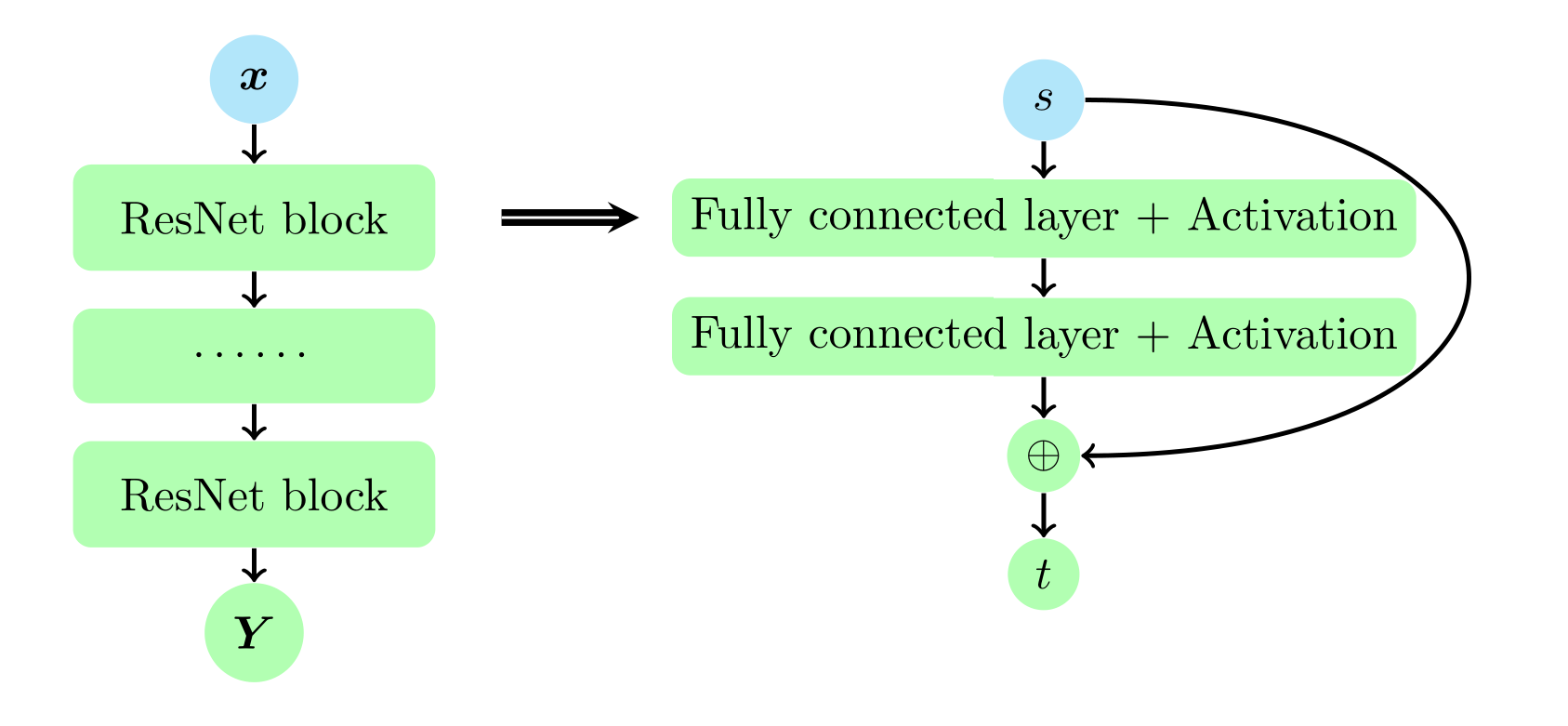
Figure 1: A schematic illustration of the Resnet networks for the construction of ${\mathscr{F}}_{\bm{\theta}_{2}}$.

Remark 3.1.

The form of the ResNet block is flexible, which may contain two or three layers, or even more layers are possible. But if the block has only a single layer, Eq (16) is in fact a linear layer, for which no advantages have been observed in [25]. The parameters $\bm{W}$ and $\bm{b}$ can be randomly initialized using the Xavier scheme (which returns truncated normal distribution with the standard deviation of $1/m$). As the choice of the activation function $\sigma$, $tanh$, $sinusoid$, $sigmoid$, etc. are possible, which will be verified and tested later in Section 5. Note that in [35], the authors remarked that for variational type method $tanh$ might be incapable of capturing some solutions.

3.2 Loss function

Let $(\bm{u}_{\bm{\theta}},w_{\bm{\theta}},p_{\bm{\theta}})$ be an approximation of the solutions of system (6)- (7) obtained with the neural networks $U_{\bm{\theta}}(\bm{x})$. We define a loss function based on the least square functional (2.1) which is written in the following form:

$$\mathscr{J}(U_{\bm{\theta}}) = \|\mathscr{L}U_{\bm{\theta}}-F\|^{2}_{(-s_{1},-s_{2},-s_{3},-s_{4})}+\alpha\|\mathscr{R}U_{\bm{\theta}}-G\|^{2}_{1/2,\Gamma}$$ (19)

where we seek $U_{\bm{\theta}}\in H^{t_{1}}(\Omega)\times H^{t_{2}}(\Omega)\times H^{t_{3}}(\Omega)\times H^{t_{4}}(\Omega)$, $\{s_{i}\}$ and $\{t_{i}\}$ are admissible values for specific boundary operators, $\alpha$ is a positive constant, and the sobolev norm $\|\cdot\|_{1/2}$ is defined as

$$\|\ell\|^{2}_{1/2,\Gamma}:=\int_{\Gamma}|\ell|^{2}d\sigma+\int\int_{\Gamma\times\Gamma}\frac{|\ell(x)-\ell(y)|^{2}}{|x-y|^{d}}d\Gamma(x)d\Gamma(y).$$ (20)

The treatment of boundary conditions is of great importance for numerical simulations. For the sake of clarity, here we take into account the boundary conditions (7) directly in the least square functional. By the trace theorem, the boundary norm is of $1/2$ order weaker than the interior norm, hence the norm $\|\cdot\|_{1/2}$ is employed. Note that the extra penalty terms due to the boundary conditions could have negative effects on the training process and the final accuracy, several efforts have been made recently for the deep neural network methods to deal with boundary conditions. For example, Liao et. al proposed a Nitche method [43] to deal with the essential boundary conditions without significant extra computational cost. Sheng et. al [54] developed a penalty free neural network methods, where they employ two networks, rather than just one, to construct the approximate solutions of the PDEs. With one networks satisfying the essential boundary conditions and the other handling the rest part of the domain, an unconstrained optimization problem is to be solved instead of a constrained one. We refer to the references above and herein [38, 49] for possible improve treatment of the boundary conditions.

Thus the VPVnet method is: find $U_{\bm{\theta}}:(x,y)\mapsto(\bm{u}_{\bm{\theta}},w_{\bm{\theta}},p_{\bm{\theta}})$ such that

$$\mathscr{J}(U_{\bm{\theta}})=\min_{\bm{\hat{\theta}}\in R^{n}}\mathscr{J}(U_{\hat{\bm{\theta}}}).$$ (21)

And we have the following remark:

Remark 3.2.

Since $\nabla\cdot\bm{u}_{\bm{\theta}}$ vanish by construction of the neural network (see section 3.1), the neural network $U_{\bm{\theta}}$ can be in fact trained by minimizing the loss function:

$$\mathscr{J}(U_{\bm{\theta}}) = \|\nu\nabla\times w_{\bm{\theta}}+\nabla p_{\bm{\theta}}-\bm{f}\|^{2}_{(-s_{1},-s_{2})}$$

$$+ \|\nu(w_{\bm{\theta}}-\nabla\times\bm{u}_{\bm{\theta}})\|^{2}_{-s_{3}}+\alpha\|\mathscr{R}U_{\bm{\theta}}-G\|^{2}_{1/2,\Gamma}.~{}~{}~{}~{}~{}~{}~{}~{}~{}~{}~{}~{}~{}~{}~{}$$

More precisely, for the pressure normal velocity boundary condition (9), we have

$$\mathscr{J}(U_{\bm{\theta}}) = \|\nu\nabla\times w_{\bm{\theta}}+\nabla p_{\bm{\theta}}-\bm{f}\|^{2}_{0}$$

$$+ \|\nu(w_{\bm{\theta}}-\nabla\times\bm{u}_{\bm{\theta}})\|^{2}_{0}+\alpha\|(\bm{u}_{n,{\bm{\theta}}},p_{\bm{\theta}})^{T}-(\bm{u}_{n}^{0},p^{0})^{T}\|^{2}_{1/2,\Gamma}.$$

For the velocity boundary condition (8), i.e. (4) , we have

$$\mathscr{J}(U_{\bm{\theta}}) = \|\nu\nabla\times w_{\bm{\theta}}+\nabla p_{\bm{\theta}}-\bm{f}\|^{2}_{0}$$

$$+ h^{-2}\|\nu(w_{\bm{\theta}}-\nabla\times\bm{u}_{\bm{\theta}})\|^{2}_{0}+\alpha\|\bm{u}_{\bm{\theta}}-\bm{g}\|^{2}_{1/2,\Gamma}.~{}~{}~{}~{}~{}~{}~{}~{}~{}~{}~{}~{}~{}~{}~{}$$

3.3 Numerical computation of loss function

We consider evaluating the loss functions (3.2) by numerical approximations, i.e. we use Gauss-Legendre quadrature rules to compute the integration of the loss functions. Once the loss function is computed, the gradient of the numerical approximation can be naturally calculated using automatic differentiation algorithm available in Tensorflow for the optimization process thereafter. Similarly as in [10], the computation make use of a partition of the domain. Let ${\mathcal{D}}_{h}$ be an uniform square grid partition of the polygonal domain $\Omega\subset\mathbb{R}^{2}$ (See figure 2). Denote by $h\coloneqq\max_{{D}\in{\mathcal{D}}_{h}}h_{D}$ the meshsize of ${\mathcal{D}}_{h}$, where $h_{D}=\operatornamewithlimits{diam}({D})$ is the diameter of the element ${D}\in{\mathcal{D}}_{h}$. Denote by ${\mathcal{E}}_{h}$ the edge set of ${\mathcal{D}}_{h}$, and ${\mathcal{E}}_{h}^{0}\subset{\mathcal{E}}_{h}$ the set of all interior edges. The set of boundary edges is denoted as ${\mathcal{E}}_{h}^{B}\coloneqq{\mathcal{E}}_{h}\backslash{\mathcal{E}}_{h}^{0}$. The diameter of the edge $e\in{\mathcal{E}}_{h}$ is denoted as $h_{e}=\operatornamewithlimits{diam}(e)$. Throughout the paper, we employ one-point Gaussian quadrature, i.e. only the element center of each grid is considered as the quadrature point. We use $\bm{x}_{D}$ and $\bm{x}_{E}$ to denote the quadrature points in element $D$ and on boundary $e$, respectively. Since the Sobolev norm $\|\cdot\|_{1/2}$ (20) is not computationally feasible, we approximate it by weighted $L^{2}$ norms with local weights $h_{e}^{-1/2}$. By (3.2), we have the following discrete loss function

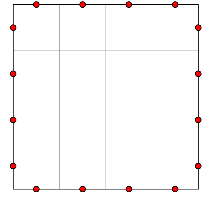
(a) QPs for boundary conditions

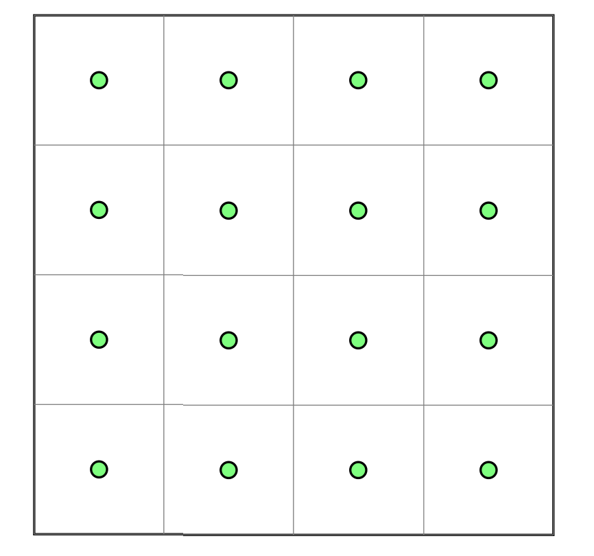
(b) QPs for residuals of equations in $\Omega$

Figure 2: A uniform partition of domain $\Omega$ and related quadrature points (QPs) for the computation of the LS functional.

$$\hat{\mathscr{J}}(\hat{U}_{\bm{\theta}}(\bm{x}))$$

$$\approx \sum_{D\in{\mathcal{D}}_{h}}\left[(p_{x}+\nu w_{y}-f^{(1)})^{2}_{(\bm{x}_{D},\bm{\theta})}+(p_{y}-\nu w_{x}-f^{(2)})^{2}_{(\bm{x}_{D},\bm{\theta})}\right]|D|$$

$$+ \sum_{D\in{\mathcal{D}}_{h}}\nu^{2}h^{-2}(w+u_{y}-v_{x})^{2}_{(\bm{x}_{D},\bm{\theta})}|D|+\alpha\sum_{e\in{\mathcal{E}}^{B}_{h}}h_{e}^{-1}(\bm{u}-\bm{g}_{D})^{2}_{(\bm{x}_{E},\bm{\theta})}|e|,$$

for the velocity boundary condition (8), where $\alpha$ is positive constants, $|D|$ and $|e|$ are the measures of element $D$ and boundary $e$. The discrete loss function for the pressure normal velocity boundary condition (9) can be derived similarly using (3.2) and will not be detailed here. The discrete VPVnet method is to find $\hat{U}_{\bm{\theta}}:(x,y)\mapsto(\hat{\bm{u}}_{\bm{\theta}},\hat{w}_{\bm{\theta}},\hat{p}_{\bm{\theta}})$ such that

$$\hat{\mathscr{J}}(\hat{U}_{\bm{\theta}})=\min_{\bm{\hat{\theta}}\in R^{n}}\hat{\mathscr{J}}(\hat{U}_{\hat{\bm{\theta}}}).$$ (26)

The discrete loss function is lower bounded by zero, since this bound is attainable for the exact solution of the Stokes’ equations, the values of the loss function reflects how well the functions $(\hat{\bm{u}}_{\bm{\theta}},\hat{w}_{\bm{\theta}},\hat{p}_{\bm{\theta}})$ approximate the solution of the Stokes’ equations. In practice, the problem (26) is solved by an iterative method, such as the stochastic gradient decent method, which will be detailed in the section of numerical experiments.

Remark 3.3.

Note that here we use Gauss-Legendre quadrature rules relying on a partition of the domain to compute the integration of the loss functions. In this way, the numerical error of evaluating the integral can be computed to a desired accuracy through either uniform or adaptive partition of the domain, which can be easily estimated and controlled. Otherwise, we can sample some points in the domain and use those sampled points to define the discrete loss function, then the method become a meshless method. For example, we sample $M_{i}$ points inside $\Omega$, $M_{\partial\Omega}$ points on $\Gamma$, and define the discrete loss function by the following weighted mean squared error,

$$\hat{\mathscr{J}}(\hat{U}_{\bm{\theta}}(\bm{x}))$$

$$\approx \sum_{M_{i}}\left[(p_{x}+\nu w_{y}-f^{(1)})^{2}_{(\bm{x}_{M_{i}},\bm{\theta})}+(p_{y}-\nu w_{x}-f^{(2)})^{2}_{(\bm{x}_{M_{i}},\bm{\theta})}\right]$$

$$+ \alpha_{2}\sum_{M_{i}}\nu^{2}(w+u_{y}-v_{x})^{2}_{(\bm{x}_{M_{i}},\bm{\theta})}+\alpha_{2}\sum_{M_{\partial\Omega}}(\bm{u}-\bm{g}_{M_{\partial\Omega}})^{2}_{(\bm{x}_{M_{\partial\Omega}},\bm{\theta})},$$

where $\alpha_{2}$ is a parameter to be determined and we adopt $\alpha_{2}=2500$ in the computation of test cased (45a) and (45b) on irregular domain (cf. Figure 7). The derivative of the discrete loss function is calculated using automatic differentiation algorithm available in Tensorflow.

4 Convergence analysis of VPVnet method

According to the universal approximation property [27], the neural networks can approximate any continuous function with small errors. Hence approximation errors of the neural network $U_{\bm{\theta}}$ can be small for any $U=(\bm{u},w,p)\in[C^{0}(\Omega)]^{4}$. In this section, we will analyze the convergence of the VPVnet method. The following is a relevant theorem [63, 5] that will be used in the demonstration:

Theorem 4.1.

Suppose that $\sigma\in C^{\infty}(R)$, $\sigma^{(\nu)}(0)\neq 0$ for $\nu=0,1,\cdots,$ and $K\subset R^{d}$ is any compact set. If $f\in C^{k}(K)$, then a function $\varphi_{n}$ represented by a DNN with complexity $n\in N$ exists such that

$$\|D^{\alpha}f-D^{\alpha}\varphi_{n}\|_{C(K)}=O\left(\frac{1}{n^{(k-|\alpha|)/d})}\omega(D^{\beta}f,\frac{1}{n^{1/d}}\right)$$ (28)

holds for all multi-indexes $\alpha$, $\beta$ with $|\alpha|\leq k$, $|\beta|=k$, where

$$\omega(g,\delta)=\sup_{x,y\in K,|x-y|\leq\delta}|g(x)-g(y)|.$$ (29)

Recall that the VPV system (6)-(7) is a uniformly bounded elliptic system in the sense of Douglis and Nirenberg. The system is well posed and has a unique solution. Hence, the minimization problem (21) has a unique solution, with the value of the infimum being 0, and the infimum is attained at the solution $U$. In this study, for simplicity, we consider only the case $s_{i}=0$ and $t_{j}=1$, and $G=0$, although the general case is similar. According to proposition 2.2, we have the following a priori estimate:

$$\|\bm{u}\|^{2}_{1}+\|w\|^{2}_{1}+\|p\|^{2}_{1}\leq C\|\bm{f}\|^{2}_{0}.$$ (30)

First, we show that when the neural network $U_{\bm{\theta}}$ and the actual solution $U$ are close to each other, we can control the loss function (19).

Theorem 4.2.

Let $U=(\bm{u},w,p)\in[H^{1}(\Omega)]^{4}$ be the solution of system (6)-(7), then there exists $U_{\bm{\theta}}:(x,y)\mapsto(\bm{u}_{\bm{\theta}},w_{\bm{\theta}},p_{\bm{\theta}})$ with $\|U-U_{\bm{\theta}}\|_{1}\leq\varepsilon$ such that

$$J(U_{\bm{\theta}})=\|\mathscr{L}U_{\bm{\theta}}-F\|^{2}_{0}+\|\mathscr{R}U_{\bm{\theta}}\|^{2}_{1/2,\Gamma}\leq c\varepsilon^{2}\text{ and }\|U_{\bm{\theta}}\|_{1}\leq\tilde{M},$$ (31)

where $c$ is a positive constant.

Proof 4.3.

We remark first that given any $\varepsilon>0$ , by Theorem 4.1, there exists a DNN $U_{\bm{\theta}}$ such that $\|U-U_{\bm{\theta}}\|_{1}\leq\varepsilon$. It follows that

$$\|\mathscr{L}U_{\bm{\theta}}-F\|^{2}_{0} = \|\mathscr{L}U_{\bm{\theta}}-\mathscr{L}U\|^{2}_{0}$$

$$\leq C^{2}_{\mathscr{L}}\|U_{\bm{\theta}}-U\|^{2}_{1}$$

$$\leq C^{2}_{\mathscr{L}}\varepsilon^{2},$$

where $C_{\mathscr{L}}$ is the operator norm bound of $\mathscr{L}$. Since $G=\bm{0}$, we also have

$$\|\mathscr{R}U_{\bm{\theta}}\|^{2}_{1/2,\Gamma} = \|\mathscr{R}U_{\bm{\theta}}-G\|^{2}_{1/2,\Gamma}$$

$$= \|\mathscr{R}U_{\bm{\theta}}-\mathscr{R}U\|^{2}_{1/2,\Gamma}$$

$$\leq C^{2}_{\mathscr{R}}\|U_{\bm{\theta}}-U\|^{2}_{H^{1}(\Omega)}\leq C^{2}_{\mathscr{R}}\varepsilon^{2},$$

where $C_{\mathscr{R}}$ is the norm bound of the boundary operator. Combining (4.3) and (4.3), we have

$$J(U_{\bm{\theta}})=\|\mathscr{L}({\mathscr{W}}_{\bm{\theta}})-F\|^{2}_{0}+\|\mathscr{R}U_{\bm{\theta}}\|^{2}_{1/2,\Gamma}\leq c\varepsilon^{2}.$$ (34)

Moreover, by (30), we have

$$\|U_{\bm{\theta}}\|_{1} \leq \|U_{\bm{\theta}}-U\|_{1}+\|U\|_{1}$$

$$\leq \varepsilon+M=\tilde{M},$$

where $M$ is the norm bound of $\bm{f}$.

Second, we show that by controlling the loss function (19), we can have an approximation $U_{\bm{\theta}}$ to the solution $U$ with small errors. The error estimate is given in the theorem below.

Theorem 4.4.

Let $U=({\bm{u}},w,p)\in[H^{1}(\Omega)]^{4}$ be the solution of system (6)-(7) and let $U_{\bm{\theta}}:(x,y)\mapsto({\bm{u}_{\bm{\theta}}},w_{\bm{\theta}},p_{\bm{\theta}})$ be such that

$$J(U_{\bm{\theta}})=\|\mathscr{L}U_{\bm{\theta}}-F\|^{2}_{0}+\|\mathscr{R}U_{\bm{\theta}}\|^{2}_{1/2,\Gamma}\leq\varepsilon^{2}.$$ (36)

Then there exists a constant $c>0$ such that

$$\|U-U_{\bm{\theta}}\|_{0}\leq\|U-U_{\bm{\theta}}\|_{1}\leq c\varepsilon.$$ (37)

Proof 4.5.

Denote $\mathscr{L}U_{\bm{\theta}}=F_{\varepsilon}$ and $\mathscr{R}U_{\bm{\theta}}=G_{\varepsilon}$. From (36), we have $\|F_{\varepsilon}-F\|_{0}\leq\varepsilon$ and $\|G_{\varepsilon}\|_{1/2,\Gamma}\leq\varepsilon$. Consider the inverse boundary operator $\mathscr{R}^{-1}:[H^{1/2}(\Gamma)]^{2}\rightarrow[H^{1}(\Omega)]^{4}$, which is linear and bounded such that $\mathscr{R}\mathscr{R}^{-1}=I$, where $I$ is the identity operator. Let ${\tilde{U}_{\bm{\theta}}}=U_{\bm{\theta}}-\mathscr{R}^{-1}G_{\varepsilon}$, we have

$$\left\{\begin{split}&\mathscr{L}\tilde{U}_{\bm{\theta}}=F_{\varepsilon}-\mathscr{L}\mathscr{R}^{-1}G_{\varepsilon},\quad{\rm in}\ \Omega,\\ &\mathscr{R}\tilde{U}_{\bm{\theta}}=0,\quad{\rm on}\ \Gamma.\\ \end{split}\right.$$ (38)

Subtracting system (38) into system (6)-(7) leads to

$$\left\{\begin{split}&\mathscr{L}\tilde{U}_{\bm{\theta}}-\mathscr{L}U=F_{\varepsilon}-\mathscr{L}\mathscr{R}^{-1}G_{\varepsilon}-F,\quad{\rm in}\ \Omega,\\ &\mathscr{R}\tilde{U}_{\bm{\theta}}-\mathscr{R}U=0,\quad{\rm on}\ \Gamma,\\ \end{split}\right.$$ (39)

Note that $\mathscr{R}^{-1}\in[H^{1}(\Omega)]^{4}$, since $\mathscr{L}$ is a fourth order elliptic operator, we have $\mathscr{L}\mathscr{R}^{-1}G_{\varepsilon}\in[H^{-3}(\Omega)]^{4}$. Then by the Lax-Milgram, we have

$$\|\tilde{U}_{\bm{\theta}}-U\|_{1}^{2}\leq C^{2}_{\mathscr{L}^{-1}}\|(F_{\varepsilon}-F)-\mathscr{L}\mathscr{R}^{-1}G_{\varepsilon}\|_{-3}^{2},$$ (40)

Therefore, we have

$$\|U_{\bm{\theta}}-U\|_{1} = \|U-(U_{\bm{\theta}}-\mathscr{R}^{-1}G_{\varepsilon})-\mathscr{R}^{-1}G_{\varepsilon}\|_{1}$$

$$\leq \|U-\tilde{U}_{\bm{\theta}}\|_{1}+\|\mathscr{R}^{-1}G_{\varepsilon}\|_{1}$$

$$\leq C_{\mathscr{L}^{-1}}\|(F_{\varepsilon}-F)-\mathscr{L}\mathscr{R}^{-1}G_{\varepsilon}\|_{-3}+C_{\mathscr{R}^{-1}}\|G_{\varepsilon}\|_{1/2,\Gamma}.$$

Since

$$\|F_{\varepsilon}-F\|_{-3}\leq\|F_{\varepsilon}-F\|_{0}\leq\varepsilon,$$ (42)

and

$$\|\mathscr{L}\mathscr{R}^{-1}G_{\varepsilon}\|_{-3}\leq C_{\mathscr{L}}\|\mathscr{R}^{-1}G_{\varepsilon}\|_{1}\leq C_{\mathscr{L}}C_{\mathscr{R}^{-1}}\|G_{\varepsilon}\|_{1/2,\Gamma}.$$ (43)

Thus

$$\|U-U_{\bm{\theta}}\|_{0}\leq\|U-U_{\bm{\theta}}\|_{1}\leq c\varepsilon,$$ (44)

The numerical error of the VPVnet method mainly comes from three parts, the approximation/expressive error caused by the deep neural network $U_{\bm{\theta}}$, the numerical error of evaluating the least square functional/neural network through numerical quadratures, and the algebraic error caused by the optimization algorithms. As shown in Theorems 4.2 and 4.4, we can obtain a neural network such that $\|U_{\bm{\theta}}-U\|\leq\varepsilon$ by minimizing the loss function (21). On the other side, the Gauss-Legendre quadrature is a classical method that is often used for approximating the value of integrals. The numerical error of evaluating the least square functional can be computed to a desired accuracy through either uniform or adaptive partition of the domain $\Omega$ and $\Gamma$ [10]. Note that common methods of optimization such as stochastic gradient descent (SGD) has been employed in this paper. Although the convergence of the optimization methods depends on many computation factors and is still a hot topic of research, as we observed in section 5, the optimization algorithm employed works well for the test cases considered.

5 Numerical experiments

The purpose of this section is two-fold. First, we shall verify the performance and accuracy of the VPVnet method on some synthetic test cases. Second, we will demonstrate the capability of the VPVnet method to approximate non-smooth/singular solutions of the Stokes’ equations, using test cases with singular solutions on L-shape domains, and a lid-driven cavity problem will be considered.

All the experiments are replicated three times to reduce variability of random initialization of the method of gradient decent and the medians of three training results are reported. The optimization algorithm is composed of two steps: we first use the Adam optimizer [36] for e.g. 5,000 iterations with self-adaptive learning rates as proposed in Tensorflow, then apply the limited-memory BroydenFletcherGoldfarbShanno algorithm with bound constraints (L-BFGS-B) [44] to finetune the results, so that errors from inexact optimization are suppressed. The training process of L-BFGS-B is terminated automatically based on the increment tolerance. Note that although both the loss functions for the pressure normal velocity boundary condition (3.2) and for the velocity boundary condition (3.2) provide satisfying numerical approximations, only numerical results obtained with the loss function (3.2) (or (3.3) in discrete form) is presented in the following, as the velocity boundary condition is most commonly used in practice. The results for the pressure normal velocity boundary condition will not be present here for simplicity.

5.1 Smooth test case

Consider the following test case defined in domains $\Omega=(0,1)^{d}$, $d=2,3$ such that (45a) and (45b) are the exact solutions. The parameter $\nu=1$ in these test cases. The external source $\bm{f}$ and the Dirichlet boundary data $\bm{g}$ is chosen such that the above functions $\bm{u}$ and $p$ are solutions to the system (1).

$$\bm{u}(x,y)=\begin{pmatrix}~{}~{}\sin(x)\sin(x)\cos(y)\sin(y)\\ -\cos(x)\sin(x)\sin(y)\sin(y)\\ \end{pmatrix},\quad p(x,y)=~{}~{}\cos(x)\cos(y),$$ (45a)

$$\bm{u}(x,y,z)=\begin{pmatrix}x+x^{2}+xy+x^{3}y\\ y+xy+y^{2}+x^{2}y^{2}\\ -2z-3xz-3yz-5x^{2}yz\\ \end{pmatrix},\quad p(x,y,z)=xyz+x^{3}y^{3}z-\frac{5}{32}.$$ (45b)

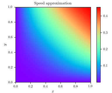
(a) Speed

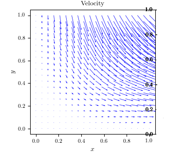
(b) Velocity

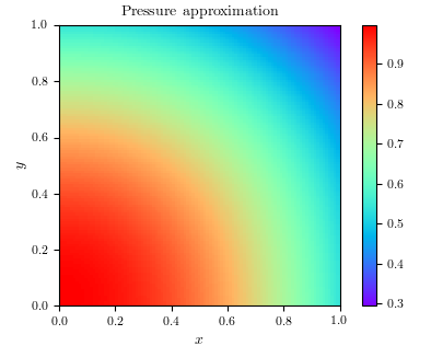
(c) Pressure

Figure 3: Numerical results of test case (45a) obtained with VPVnet method using $20\times 20$ uniformly distributed quadrature points in $\Omega{=(0,1)^{2}}$.

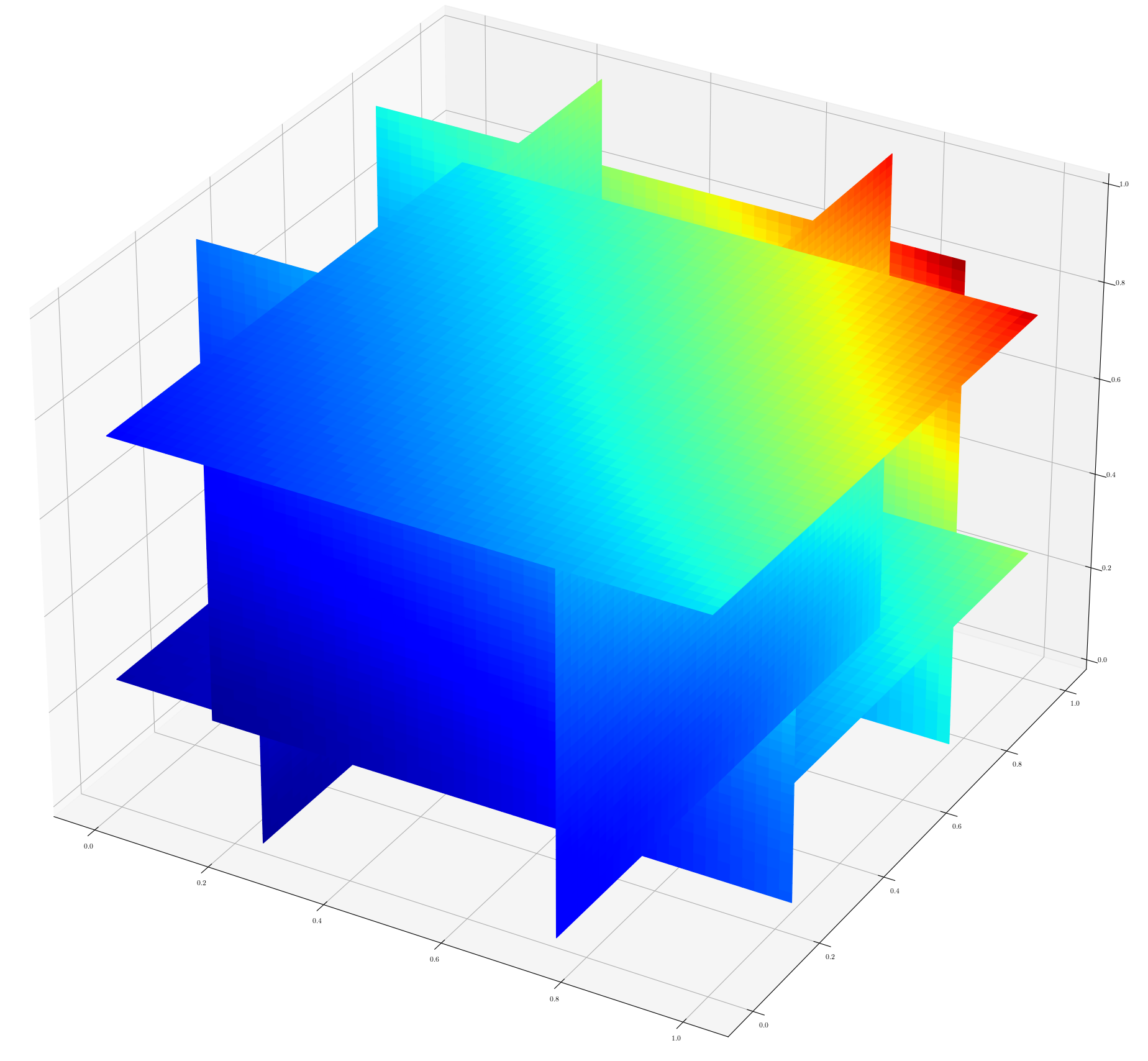
(a) Speed

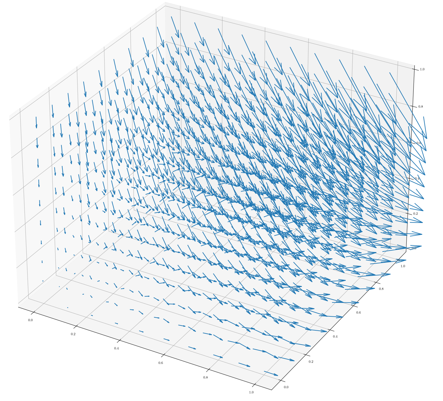
(b) Velocity

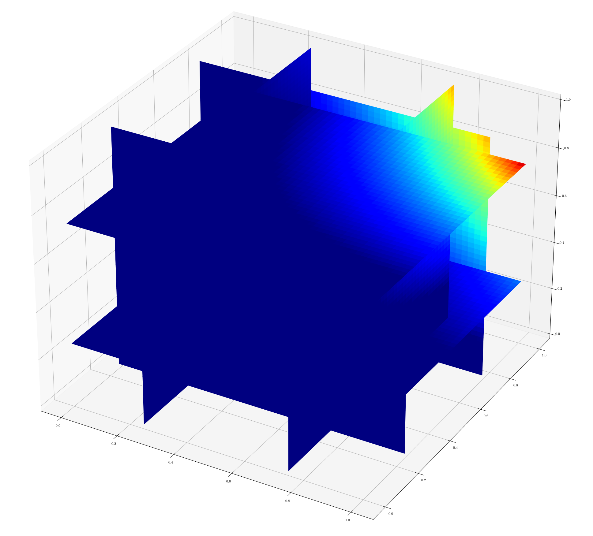
(c) Pressure

Figure 4: Numerical results of test case (45b) in 3D obtained with VPVnet method using $20\times 20\times 20$ uniformly distributed quadrature points in $\Omega{=(0,1)^{3}}$.

We first examine the accuracy of the VPVnet method by varying the number of quadrature points and the number of layers and neurons. We use neural networks of different structures to approximate the solution of the Stokes’ problem (45a). For example, a neural network comprised of $2$ Resnet blocks, i.e. $4$ hidden layers, and each hidden layer admits $8$ neurons, with total $267$ trainable parameters, is one of the neural networks considered. For simplicity, we note the neural networks by its number of hidden layers $N_{L}$ and the number of neurons $N_{N}$ within each hidden layers, hence the above neural network is noted as a neural network of $4\times 8$. We also use neural networks of $8\times 8$, $4\times 16$, $8\times 16$ hidden layers and neurons, with total $555$, $915$, $2003$ trainable parameters, respectively, to approximates the solutions of the model problem (45a).

The discrete loss functions (3.3) is considered for the VPVnet method. The quadrature points (QPs) for the evaluation of the loss function is uniform grid data on the domain, one point quadrature rules is considered, which consist of $50\times 50$ (or $20\times 20$) points in total. Hence we have $h=1/50$ (or $h=1/20$). And we choose $\alpha=1$. QPs for the boundary condition of $u$, $v$ is uniformly distributed points on the boundary of $\Omega$ , which contains $50$ (or $20$) points on each edge, i.e $200$ (or $80$) points in total. An illustration of these QPs is shown in Fig 2. As mentioned previously, the optimization problem is first computed with 2000 Adam iterations, and followed by at most 5000 L-BFGS-B iterations, the learning rates are determined by existing self-adaption algorithms in Tensorflow.

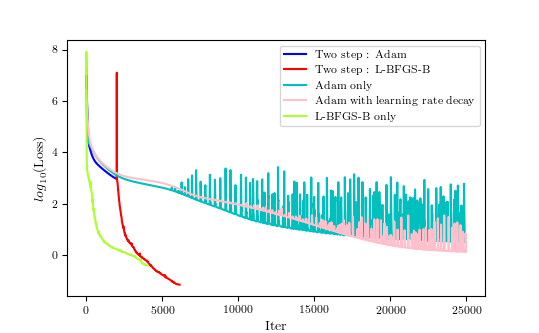
(a) Convergence of loss for test case 5.1(a)

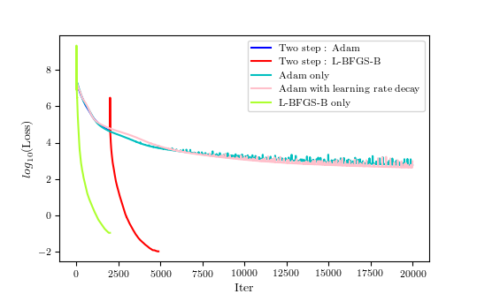
(b) Convergence of loss for test case 5.1(b)

Figure 5: Convergence of loss function over optimization iteration with different optimization processes for test case 5.1(a) and 5.1(b), the curves are: $(1)$ Two step optimization : Adam part; $(2)$ Two step optimization : L-BFGS-B part;$(3)$ Adam optimizer only; $(4)$ Adam optimizer with a hyperparameter of learning rate $5e-4$ with exponential decay rate 0.98; $(5)$ L-BFGS-B optimizer only.

Figure 5 is the convergence of loss function over different optimization iterations. As we can observe both in Fig. 12(a) and 12(b), the two-step approach allow a much faster convergence and even a better precision than just using Adam only. This is because BFGS uses the Hessian matrix (curvature in highly dimensional space) to calculate the optimization direction and provides more accurate results. However, if BFGS is used directly without using the Adam optimizer, the optimization can rapidly converge to a local minimum [47]. For this reason, the Adam optimizer is used first to avoid local minima, and then the solution is refined by BFGS. Here we use the L-BFGS-B method instead of the BFGS method in our work.

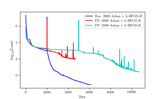
Figure 6: Convergence of loss function over optimization iterations obtained with different neural network structures for test case 5.1(a): $(1)$ neural network with Resnet blocks, 2000 Adam optimization iteration plus L-BFGS-B optimization process; $(2)$ feedforward neural network, 2000 Adam optimization iteration plus L-BFGS-B optimization process; $(3)$ feedforward neural network, 5000 Adam optimization iteration plus L-BFGS-B optimization iterations.

Figure 6 show the convergence of loss function over optimization iteration obtained with two different neural network structures for test case 5.1(a), the first is neural network with Resnet (Res) blocks, the second is feedforward (FF) neural network, note that these two neural networks have the same number of 8 hidden layers and each hidden layers have the same number of 20 neurons, except that the neural network with Resnet blocks has a residual connection every two layers. We can see that the neural network with Resnet blocks converges faster and gives a better precision than classical feedforward network. Hence neural network with Resnet blocks is adopted for all the subsequent test cases in this work.

Table 1: Numerical errors of the VPVnet method for test case (45a).

Network	VPVnet method
$N_{L}N_{N}$	$20\times 20$ Quadrature points			$50\times 50$ Quadrature points
	$e_{u}$	$e_{v}$	$e_{p}$	$e_{u}$	$e_{v}$	$e_{p}$
$4\times 8$	7.88e-4	8.08e-4	1.36e-2	7.27e-4	7.58e-4	5.16e-3
$8\times 8$	8.35e-4	8.26e-4	6.62e-3	5.09e-4	5.45e-4	3.31e-3
$4\times 16$	6.58e-4	5.50e-4	1.02e-2	3.46e-4	4.47e-4	5.71e-3
$8\times 16$	5.24e-4	5.49e-4	4.56e-3	4.34e-4	4.99e-4	5.51e-3

The numerical approximations obtained with the VPVnet method (using $sinusoid$ activation function) for the speed, velocity and pressure are plotted in Figure 3. The $L_{2}$ numerical errors of each variable $u,v,p$ are presented in Table 1. We observe that for this smooth test case, we can have a rather good approximation with a small number of hidden layers and neurons. Although the numerical error varies due to the variability of random initialization of the parameters, we can observe that by using either more hidden layers, more number of neurons or more quadrature points, a tendency of better precision can be observed within certain limits.

Table 2: Numerical error of the VPVnet method for test case (45a) using different activation function, a neural network of $8\times 16$ hidden layers and neurons, and $50\times 50$ quadrature points.

Activation	VPVnet method
function	$e_{u}$	$e_{v}$	$e_{p}$
$Sin$	4.34e-4	4.99e-4	5.51e-3
$Tanh$	5.11e-4	5.20e-4	9.98e-3
$Sigmoid$	3.01e-3	3.36e-3	1.59e-2

Table 2 shows the $L_{2}$ numerical errors using different activation functions. The errors are obtained using a neural network with $8\times 16$ hidden layers and neurons, and $50\times 50$ quadrature points. The results obtained with activation functions $Sin(x)$, $Tanh(x)$ and $Sigmoid(x)$ are all of satisfying precision. We remark that the one of most commonly used activation function $ReLU$ is not considered here, since the function is not differentiable everywhere, while first-order derivative is presented in the loss functions and we use the automatic differentiation, i.e tf.gradient() to approximate the derivative, which will cause problems. A possible remedy to this problem might be using $max(0,x^{3})$ instead of $ReLU:=max(0,x)$ as proposed in [19]. Or we can approximate the derivative by using the finite difference quotient, as did by Cai $et$ $al.$ in [10]. The choice of finite difference quotient for the approximation of the derivative of different variable in $2D$ or $3D$ is a question that needs careful consideration. For the sake of clarity, we avoid such investigations here. In the rest of this paper, without specification, we will use $Sin(x)$ as the activation function.

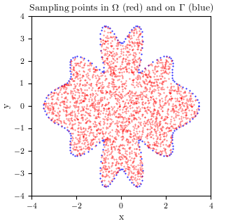
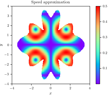
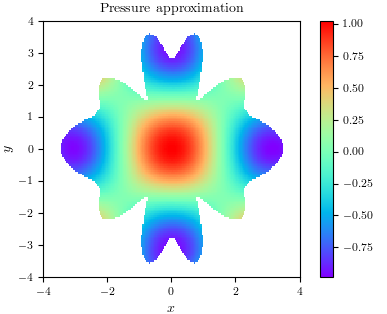
(a) Sampling points, speed approximation and pressure approximation for 2D test case 5.1(a)

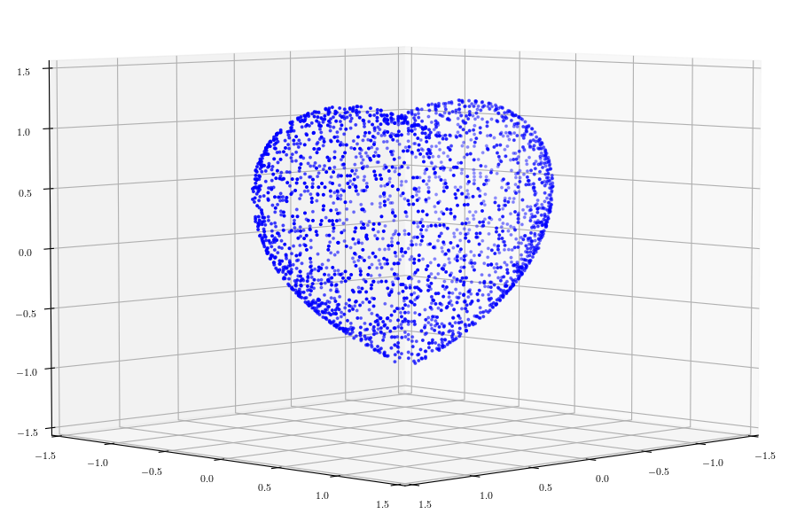
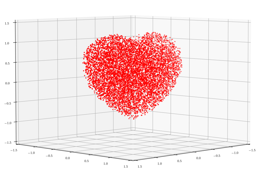
(b) Sampling points on the boundary (left) and inside the domain (right) for 3D test case 5.1(b)

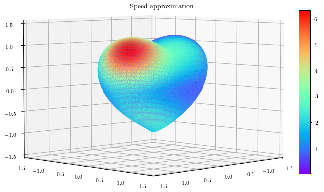
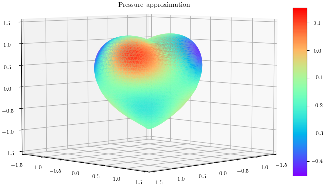
(c) Speed approximation and pressure approximation for 3D test case 5.1(b)

Figure 7: Numerical results of test case (45a) and test case (45b) obtained with VPVnet method using random sampling points in irregular domains

We use neural networks of $8\times 16$ hidden layers and neurons to approximate the solution of the 3D test case (45b). The quadrature points for the evaluation of the loss function is uniform grid data in the cube domain, which consist of $20\times 20\times 20$ points in total. Note that BFGS instead of the L-BFGS-B algorithm is used to finetune the results obtained with the Adam optimizer in this 3D test case, as a better precision can be achieved by using the former. The $L_{2}$ numerical errors obtained with the VPVnet method (using $sinusoid$ activation function) is $1.24e-5$, $1.37e-5$, $1.37e-5$, $4.85e-5$, $4.95e-3$, for variable $(\bm{u},p)$, where $\bm{u}=(u^{(1)},u^{(2)},u^{(3)})^{T}$ in 3D, respectively. Similar precisions are reached for $tanh$ and $sigmoid$ activation functions, which will not be listed here for simplicity. The numerical approximations obtained with the VPVnet method for the speed, velocity and pressure are plotted in Figure 4. The numerical results show that VPVnet method is accurate and efficient in 3D.

The test cases (45a) and (45b) have been performed on more complex geometries using random sampling points. In this case, the loss function (3.3) is employed. The test case (45a) is preformed on a butterfly-like domain $\Omega$. The boundary $\Gamma$ of the domain $\Omega$ is defined by the following equation [56]:

$$\Gamma(x,y)=\left\{{(x,y)}^{T}\in R^{2}:\;x(\theta)=r(\theta)cos(\theta),\;y(\theta)=1.4r(\theta)sin(\theta),\;\theta\in[0,2\pi]\right\},$$

where $r(\theta)=2\sqrt{cos^{2}(5\theta)+cos^{2}(2\theta)+cos^{2}(\theta)}$. We used $200$ and $2500$ random sampling points (cf Fig. 7(a)), respectively, on the boundary and inside of the computation domain. As for the 3D test case (45b), the domain boundary is described by the zero iso-value of the function $\phi$ [24]:

$$\Gamma(x,y,z)=\left\{{(x,y,z)}^{T}\in R^{3}:\;\phi(x,y,z)=\left(x^{2}+\tfrac{9}{4}y^{2}+z^{2}-1\right)^{3}-x^{2}z^{3}-\tfrac{9}{80}y^{2}z^{3}=0\right\}.$$

$2500$ and $8000$ random sampling points are employed (cf Fig. 7(c)), respectively, on the boundary and inside of the computation domain. Convergence can be easily obtained for both test cases using the same optimization processes as previously used. The numerical results (cf Fig. 7) show that the method is very flexible on complex geometries. The $L_{2}$ numerical errors obtained with the VPVnet method (using $sinusoid$ activation function) is $3.20e-03$, $3.16e-03$ and $3.34e-02$ for variable $(\bm{u},p)$, where $\bm{u}=(u^{(1)},u^{(2)})^{T}$ in 2D, respectively (and $5.88e-05$, $1.30e-04$, $2.58e-05$, $7.77e-3$ for $(\bm{u},p)$ in 3D). The precision can be further improved by adaptive sampling [62] which is the subject for future study.

5.2 Pressure-robust test case

In this example, let $\Omega=(0,1)^{2}$, and choose the proper right-hand side function such that the following functions satisfy system (1).

$$\bm{u}(x,y)=\begin{pmatrix}-e^{x}(y\cos(y)+\sin(y))\\ ~{}~{}e^{x}y\sin(y)\\ \end{pmatrix},\quad p(x,y)=2e^{x}\sin(y).$$ (46)

Since $-\Delta\bm{u}=(-2e^{x}\sin(y),-2e^{x}\cos(y))^{t}$, it is easy to check that when $\nu=1$, we have a homogeneous equation with $\bm{f}=0$. When $\nu=0$, $\bm{f}$ is a nonzero function. It is well known that the classical finite element methods, such as the mini element, Taylor-Hood element, etc, suffer from a common lack of robustness when $\nu\ll 1$. The velocity error can become extremely large. It is also called poor mass conservation sometimes, since for $H^{1}$-conforming mixed methods such large velocity errors are accompanied by large divergence errors. In this test case, we will report the robustness results of the VPVnet method.

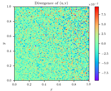
(a) $\nu=1e-2$

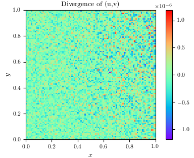
(b) $\nu=1e-4$

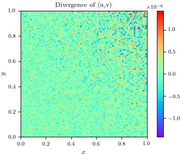
(c) $\nu=1e-6$

Figure 8: Numerical results of divergence of $\bm{u}$ for test case (46) obtained with VPVnet method using $50\times 50$ uniformly distributed quadrature points in $\Omega$.

Table 3: Numerical error of the VPVnet method with different value of $\nu$ for test case (46), using a neural network with $8\times 16$ hidden layers and neurons, and $20\times 20$ and $50\times 50$ quadrature points.

	VPVnet method
$\nu$	$20\times 20$ Quadrature points			$50\times 50$ Quadrature points
	$e_{u}$	$e_{v}$	$e_{p}$	$e_{u}$	$e_{v}$	$e_{p}$
$1e-2$	4.18e-4	1.35e-3	1.46e-3	1.60e-4	5.86e-4	2.62e-3
$1e-4$	2.06e-4	5.94e-4	1.89e-3	2.26e-4	7.78e-4	2.85e-3
$1e-6$	3.22e-4	9.23e-04	8.68e-4	3.98e-4	1.18e-3	2.09e-3

The numerical experiments are carried out for $\nu=1e-2,\;1e-4,\;1e-6$. The numerical results are obtained using a neural network with $8\times 16$ hidden layers and neurons, and $20\times 20$ and $50\times 50$ quadrature points. The optimization problem is computed with 2000 Adam and at most 5000 L-BFGS-B iterations, respectively. The $L_{2}$ numerical errors obtained with the VPVnet method of variable $u,v,p$ are presented in Table 3. We obtain very good approximations of the solutions for any value of $\nu$, including the value $\nu$ very small. The divergence of the velocity $div\bm{u}=u_{x}+v_{y}$ for different values of $\nu$ is plotted in Figure 8. Hence the VPVnet method is divergence-free and pressure-robust.

5.3 Smooth test case on L-shape domain

For further examination, the more complicated domain, L-shape domain, is considered to validate in this research. The domain is defined by $\Omega=(-1,1)^{2}\backslash([0,1]\times[-1,0])$. It is called the backward facing step domain of flow problems. The parameter $\nu$ is of value $1$ for all domain, $\nu=1$. The test case is of exact solution as shown in Eq. (46). The same test case has been considered in [59] and many other references.

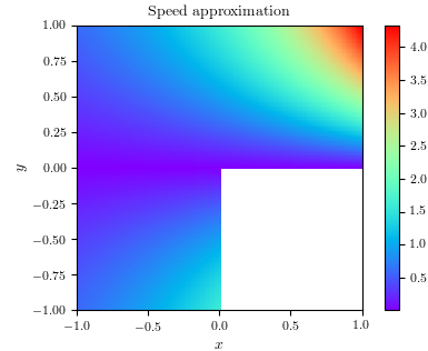
(a) Speed

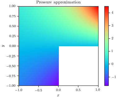
(b) Pressure

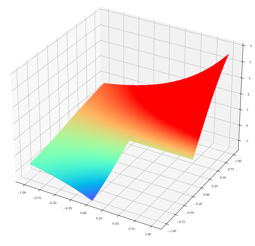
(c) Pressure plot in 3D

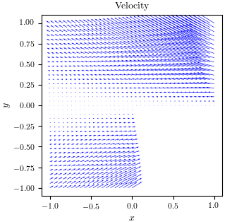
(d) Velocity

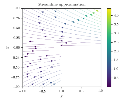
(e) Streamline

Figure 9: Numerical results of test case (46) on L-shape domain obtained with VPVnet method using nearly $50\times 50\times 3$ uniformly distributed quadrature points in $\Omega$.

We obtain good approximations for the test case on L-shape domain with the VPVnet method. Note that the test case has the same exact solution as (46) in subsection 5.2, hence similar computation configuration has been used and the numerical errors are not shown here again. The numerical approximations obtained with the VPVnet method for the speed, velocity, pressure and the streamline are plotted in Figure 9.

5.4 Singular test case on L-shape domain

Hereafter, we consider a singular solution on the L-shaped domain $\Omega:=(-1,1)^{2}$$\backslash$$[0,1)\times(-1,0]$. The test case is proposed by Verfürth in [58] and has been widely used in the literature [14, 41]. Let $\omega=3\pi/2$, ${\delta}=0.5444837$. Given $(r,\theta)$ the polar coordinates at the re-entrant corner $(0,0)$, introduce the auxiliary function

$$\psi(r,\theta)=\frac{\sin((1+{\delta})\theta)\cos({\delta}\omega)}{1+{\delta}}-\cos((1+{\delta})\theta)-\frac{\sin((1-{\delta})\theta)\cos({\delta}\omega)}{1-{\delta}}+\cos((1-{\delta})\theta).$$ (47)

The singular solution we approximate is

$$\left\{\begin{split}&u(x,y)=r^{{\delta}}\left((1+{\delta})\sin(\theta)\psi(\theta)+\cos(\theta)\psi^{\prime}(\theta)\right),\\ &v(x,y)=r^{{\delta}}\left(\sin(\theta)\psi^{\prime}(\theta)-(1+{\delta})\cos(\theta)\psi(\theta)\right),\\ &p(x,y)=r^{{\delta}-1}\left((1+{\delta})^{2}\psi^{\prime}(\theta)+\psi^{(3)}(\theta)\right)/(1-{\delta}).\end{split}\right.$$ (48)

The Stokes equation is homogeneous with this solution, i.e $\bm{f}=0$. Moreover, the Dirichlet conditions are homogeneous along the edges except at the re-entrant corner. We emphasize that the pair $(\bm{u},p)$ is analytical in $\Omega\backslash(0,0)$, but $\nabla\bm{u}$ and $p$ are singular at the origin. Especially, $\bm{u}\notin[H^{2}]^{2}(\Omega)$ and $p\notin H^{1}(\Omega)$. This solution reflects perfectly the typical behavior of the solution of the Stokes problem near a reentrant corner. In general, for solution $(\bm{u},p)$ to the Stokes problem in a non-convex domain $\Omega$, we can expect $\bm{u}\in[H^{s}(\Omega)]^{2}$ and $p\in H^{s-1}$ for $s<1+{\delta}$. Hence the solution $\bm{u}$ is in $C^{0}$, and theoretically, the neural networks is capable of approximating a $C^{0}$ function at any error. It is expected by construction that the VPVnet method can capture such singular solutions, which is confirmed by the following numerical results.

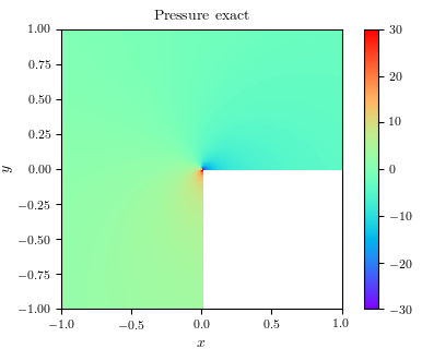
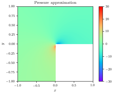
(a) Exact(left) & approximate(right) pressure for domain $(-1.0,1.0)^{2}$

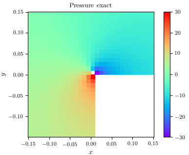
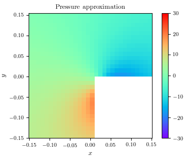
(b) Exact(left) & approximate(right) pressure(zoom) domain $(-0.15,0.15)^{2}$

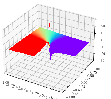
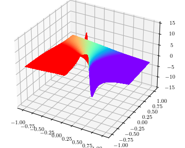
(c) Exact & approximate pressure plot in 3D

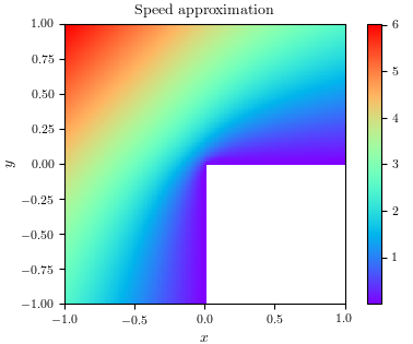
(d) Speed

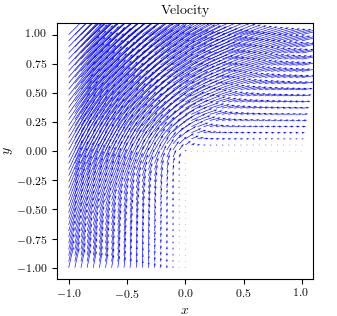
(e) Velocity

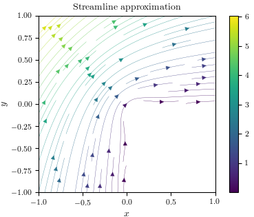
(f) Streamline

Figure 10: Numerical results of test case (48) obtained with VPVnet method using $50\times 50\times 3$ quadrature points in $\Omega$.

Table 4: Error of the VPVnet method for test case (48) using $8\times 16$ hidden layers and neurons.

Quadrature	VPVnet method
points	$e_{u}$	$e_{v}$	$e_{p}$
$20\times 20\times 3$	2.75e-2	2.22e-2	5.21e-1
$50\times 50\times 3$	6.45e-3	5.92e-3	1.96e-1
$100\times 100\times 3$	8.60e-3	8.63e-3	3.17e-1

The computation configuration is as follows: The parameters $\alpha=1$ and a neural network with $12\times 16$ hidden layers and neurons is employed for all experiments in this test case. Uniform partitions of size $20\times 20\times 3$, $50\times 50\times 3$ and $100\times 100\times 3$ are considered. (Note that we use $*\times*\times 3$ QPs because the L-shape domain is composed of 3 square domain.) One point quadrature rules is employed for all cases. Hence we have $h=1/20$ (or $h=1/50$, $h=1/100$) for the uniform partitions. As for the boundary condition of $u$, $v$, the partition is in accordance with the partitions interior domain. For the optimization, $2000$ Adam iteration is used, while more L-BFGS-B iterations is needed (less than 50000 iterations), respectively.

The numerical solutions obtained with the VPVnet method for the speed, velocity, pressure and the streamline, and the exact solution for the pressure are are plotted in Figure 10. The numerical results in Table 4 clearly show that the VPVnet method can provide good approximations for $\bm{u}\in[H^{s}(\Omega)]^{2}$, $2>s>1$. While the errors obtained with the VPVnet method for $p\in H^{s-1}$, $2>s>1$ are much larger, due to the strong pressure singularities near the re-entrant corner $(0,0)$, which can also be observed in Figure 10(a), 10(b) and 10(c). The numerical errors can be reduced by refinement within a certain limit, then it will not get any better, indicating more efforts are needed to reach a satisfying precision. Recall that only smooth activation function is considered here in this paper, and it has been shown in [10] that the piecewise activation functions, e.g. $Leaky$ $ReLU$ gives a better performance than the smooth activation functions for a interface problem, hence it would be interesting to try continuous piecewise activation functions as remarked in subsection 5.1, which is subject to further investigations.

5.5 Lid-driven cavity test cases

The lid-driven cavity test case has been used as a benchmark problem for many numerical methods due to its simple geometry and complicated flow behaviors [8]. The computation domain is $\Omega=(0,1)^{2}$ in 2D. And the Dirichlet boundary condition is given as $\bm{u}_{\Gamma}=\bm{g}=(1,0)^{T}$ for $y=1$ and $\bm{g}=(0,0)^{T}$ on the rest of the boundary.

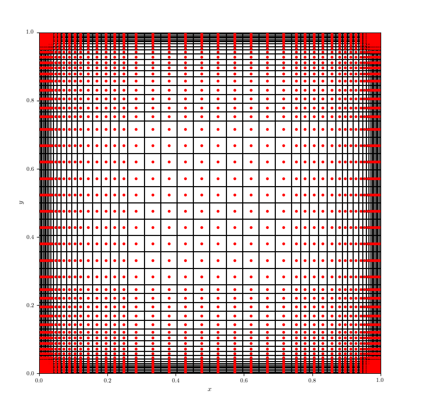
(a) Quadrature points in 2D

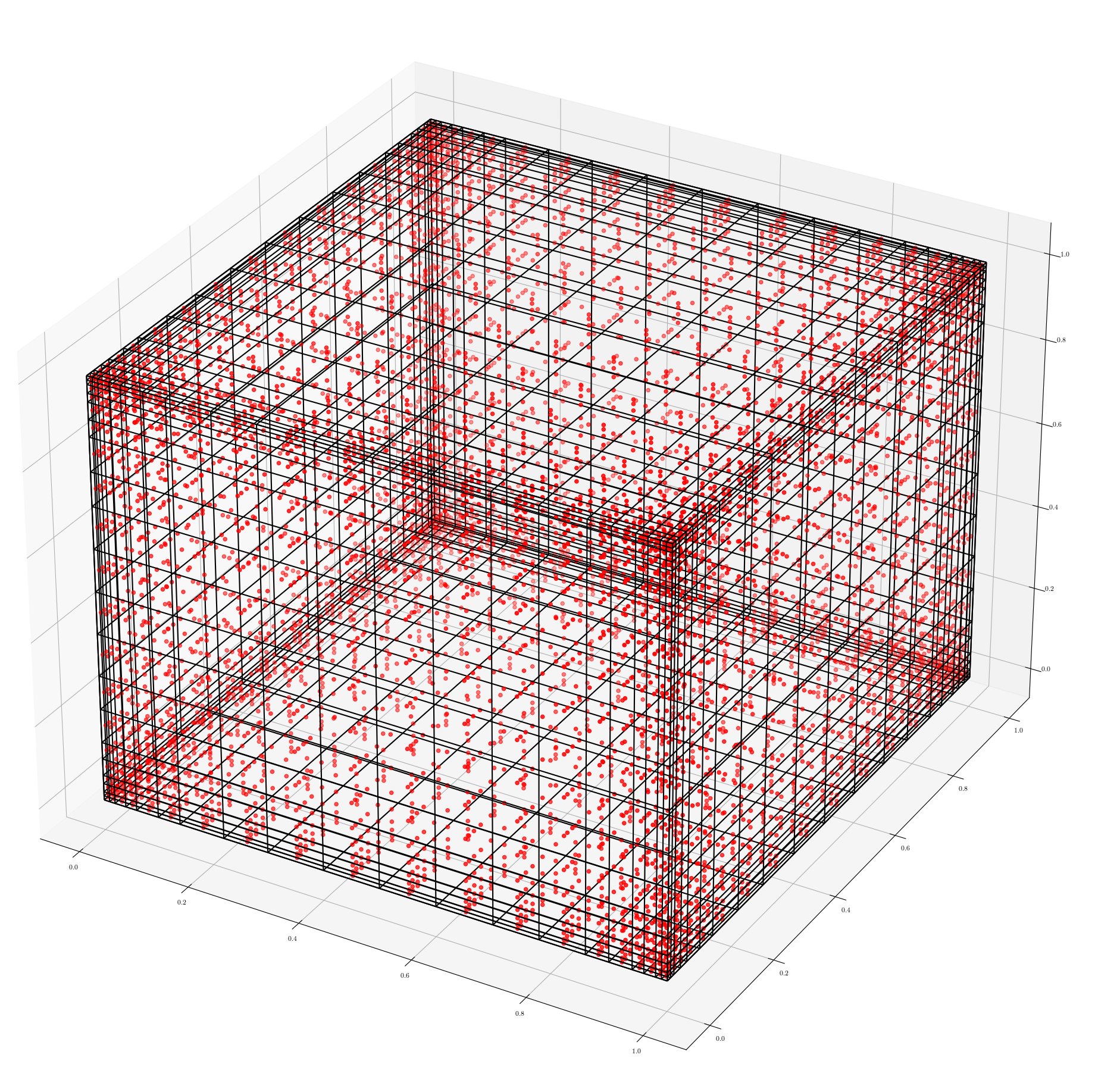
(b) Quadrature points in 3D

Figure 11: Local refined quadrature points of lid-driven cavity test case used for VPVnet method.

The main difficulty of this problem comes from the presence of singularities at corners of the domain. The pressure and the vorticity are not finite at the two top corners of the domain. Singularities also present at the corners $(0,0)$ and $(1,0)$, where the second derivative of the velocity is unbounded, which is weaker than the previous ones. By calculating the norm, one can see that $\bm{g}\in H^{1/2-\delta}(\partial\Omega,R^{2})$ for all $0<\delta<1/2$ but $\bm{g}\notin H^{1/2}$, hence the velocity is not in $H^{1}$. Thus the usual variational formulation for the Stokes’ problem does not apply for the lid-driven cavity problems. However, this test case is used in many papers to test finite elements methods and the discontinuous boundary condition is usually applied directly to the finite element discretization in practice. In fact, on one hand, we can approximate the discontinuous boundary data by a smooth one and then apply a finite element method to the regularized problem, on the other hand, it has been observed that for properly defined continuous boundary condition, the discrete system will not see the difference between the discontinuous and the continuous boundary condition [10, 18]. In this paper, we expect to explore the capacity of the VPVnet method to solve this problem.

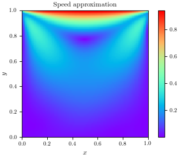
(a) Speed

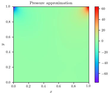
(b) Pressure

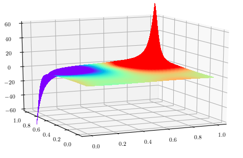
(c) Pressure plot in 3D

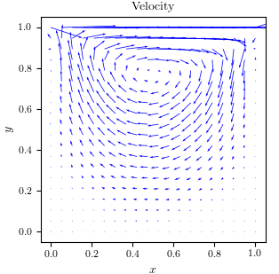
(d) Velocity

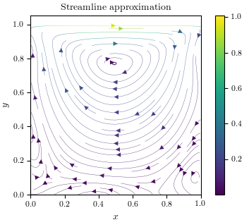
(e) Streamline

Figure 12: Numerical results of lid-driven cavity test case obtained with VPVnet method using $50\times 50$ locally refine quadrature points in $\Omega$.

We use the following computation configuration for 2D case computation: the parameters $\alpha=1$ and a neural network with $12\times 16$ hidden layers and neurons is employed. A locally refined partition of size $50\times 50$ which is geometrically refined towards all the corners, i.e. $(0,0)$, $(1,0)$, $(0,1)$ and $(1,1)$, are considered. The locally refined partition has elements of size varies from $4.0e-3$ to $4.8e-2$, an illustration is shown in Fig 11(a). One point quadrature rules is employed. We pick the value of $h=1/50$. As for the boundary condition of $u$, $v$, the partition is in accordance with the partitions interior domain, i.e. locally refined points on the boundaries of $\Omega$ are used. The discontinuous boundary condition is applied directly.

The numerical approximations obtained with the VPVnet method of the speed, velocity, pressure and the streamline for the lid-driven cavity test case are plotted in Figure 12. The exact solution of lid-driven problem is not known for the Stokes’ problem. The shape of streamlines is similar to the result given in [41], strong pressure singularities are present at the top two corners, the results look quite reasonable. Note that, there are some perturbations which can be observed near the domain boundaries, particularly in the figure for the streamline 12(e). We refine the partition of the domain by $200\times 200$ rectangular element with size from $1.0e-3$ to $8.0e-3$. The perturbations turns to diminish (see Fig. 13).

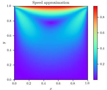
(a) Speed

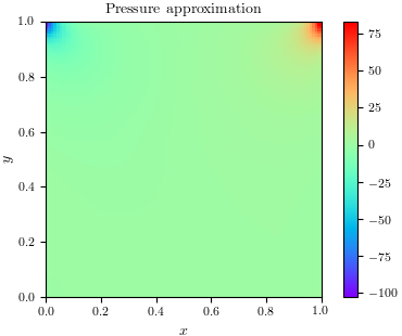
(b) Pressure

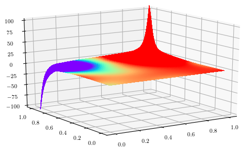
(c) Pressure plot in 3D

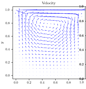
(d) Velocity

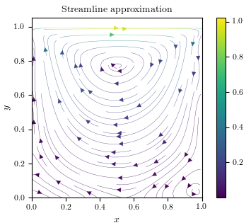
(e) Streamline

Figure 13: Numerical results of lid-driven cavity test case obtained with VPVnet method using $200\times 200$ locally refine quadrature points in $\Omega$.

We also consider the 3D lid-driven cavity test case in a unit cubic domain. A tangential velocity $\bm{u}_{\Gamma}=(1,0,0)^{T}$ is imposed at the top surface of the domain, while $\bm{u}=(0,0,0)^{T}$ is imposed on the rest of the boundary. The parameters $\alpha=1$ and a neural network with $16\times 16$ hidden layers and neurons is employed for the computation. Locally refined partitions of size $10\times 10\times 10$ and $20\times 20\times 20$ which are geometrically refined towards the domain corners are considered. The locally refined partition has elements of size varies from $2.0e-2$ to $2.0e-1$ for the $10\times 10\times 10$ partition, and $1.0e-2$ to $1.0e-1$ for $20\times 20\times 20$ partition, an illustration is shown in Fig. 11(b). Note that for 3D computation, the BFGS algorithm is used to finetune the results obtained with 2000 Adam optimization iterations. The numerical results are shown in Figures 14 and 15, where Figure 15 show the top view along the $x,y,z$ axis respectively. The numerical results indicate that the VPVnet method is efficient and accurate.

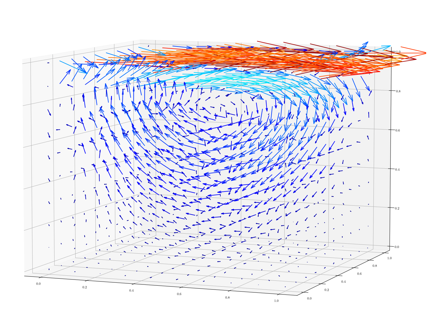
(a) velocity with 1000 QPs

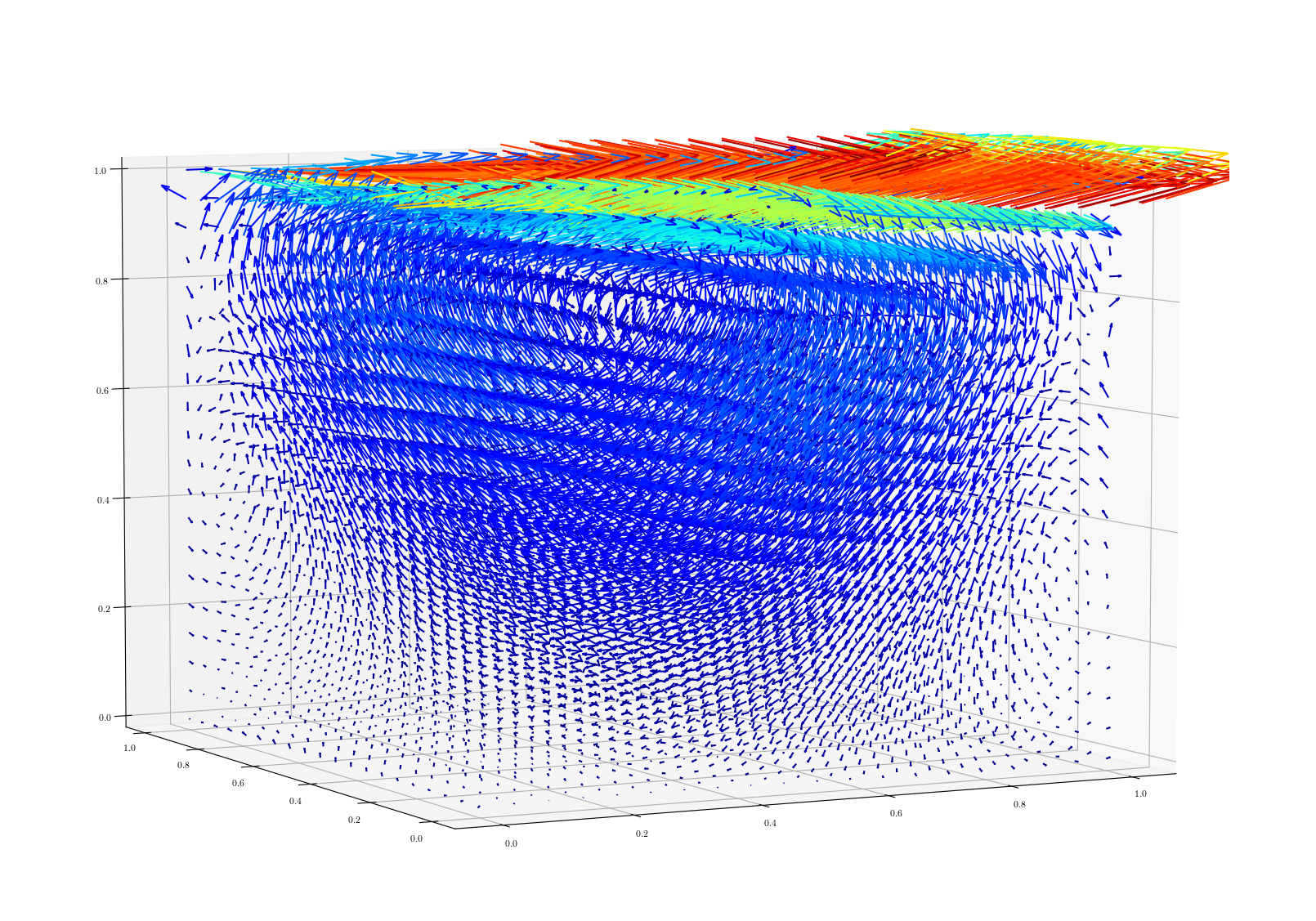
(b) velocity with 8000 QPs

Figure 14: Numerical results of 3D lid-driven cavity test case obtained with VPVnet method using $1000$ and $8000$ locally refine quadrature points in $\Omega$.

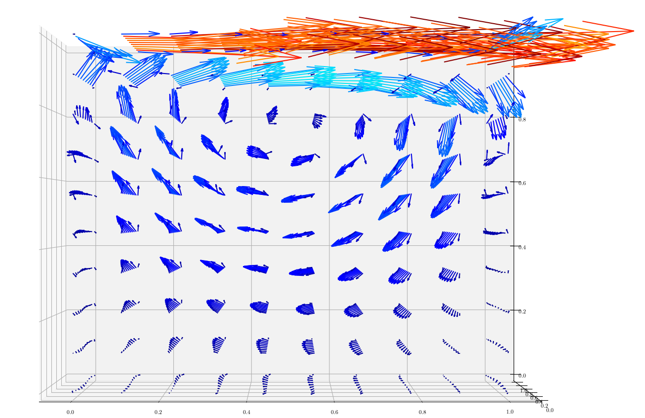
(a) view from x-axis

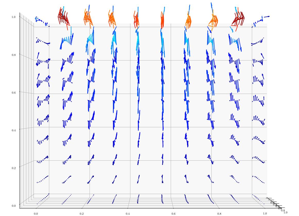
(b) view from y-axis

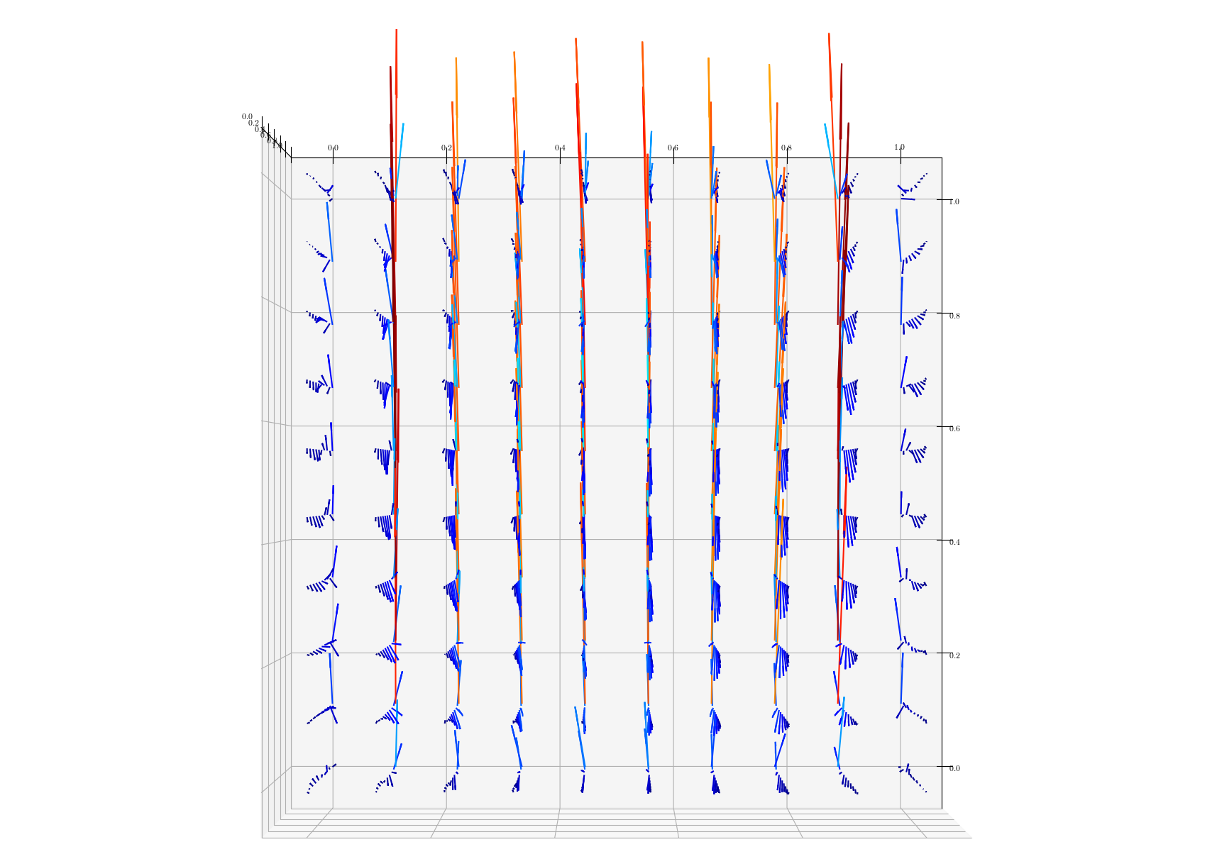
(c) view from z-axis

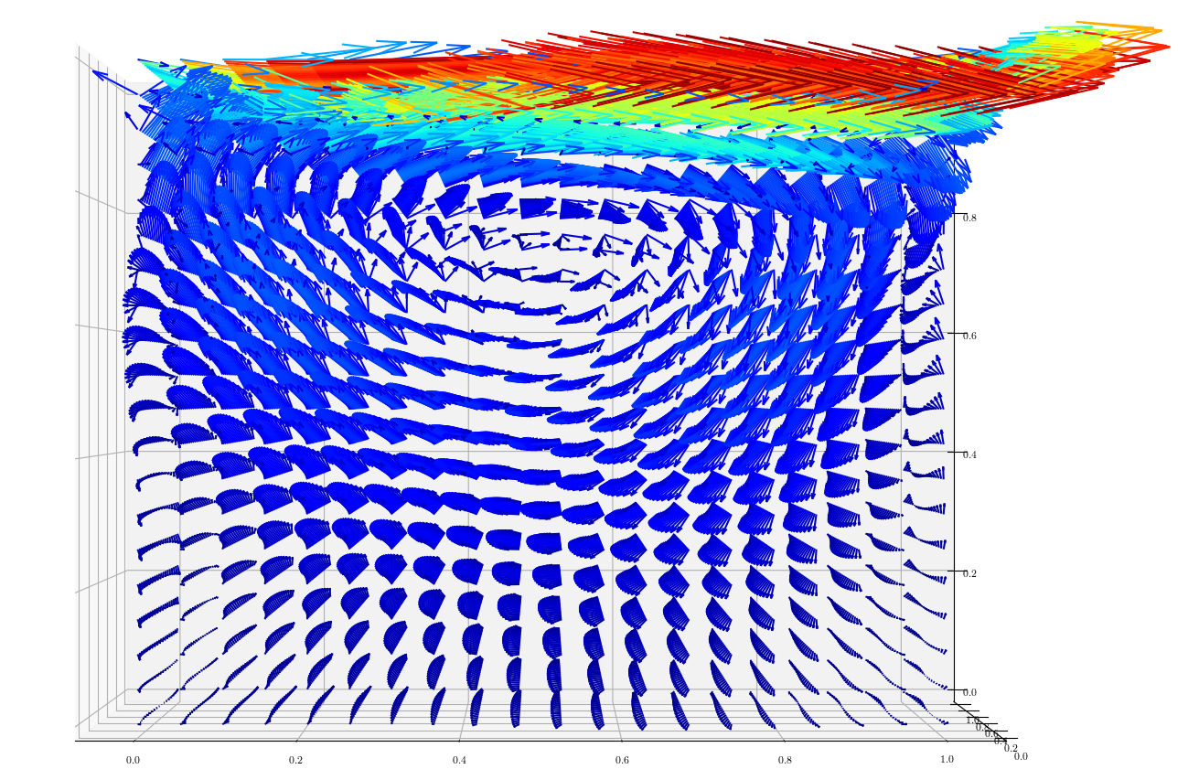
(d) view from x-axis

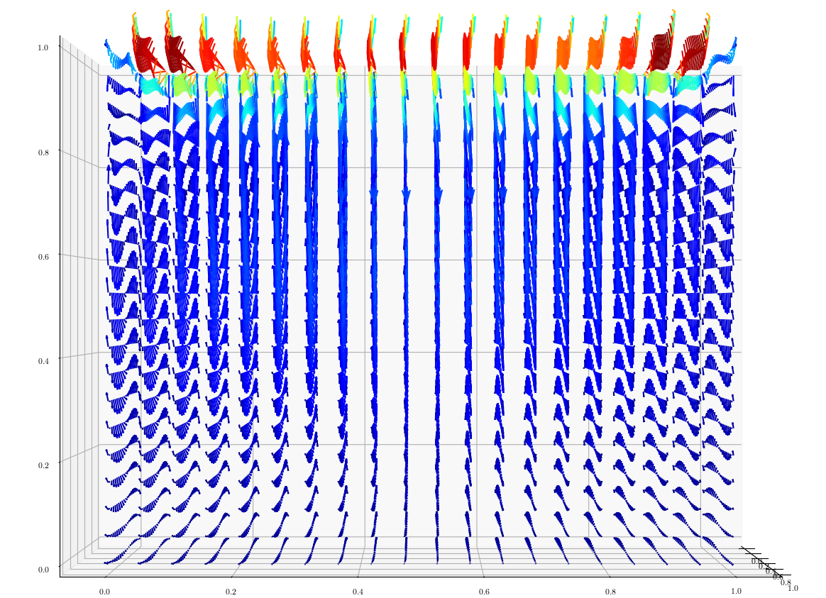
(e) view from y-axis

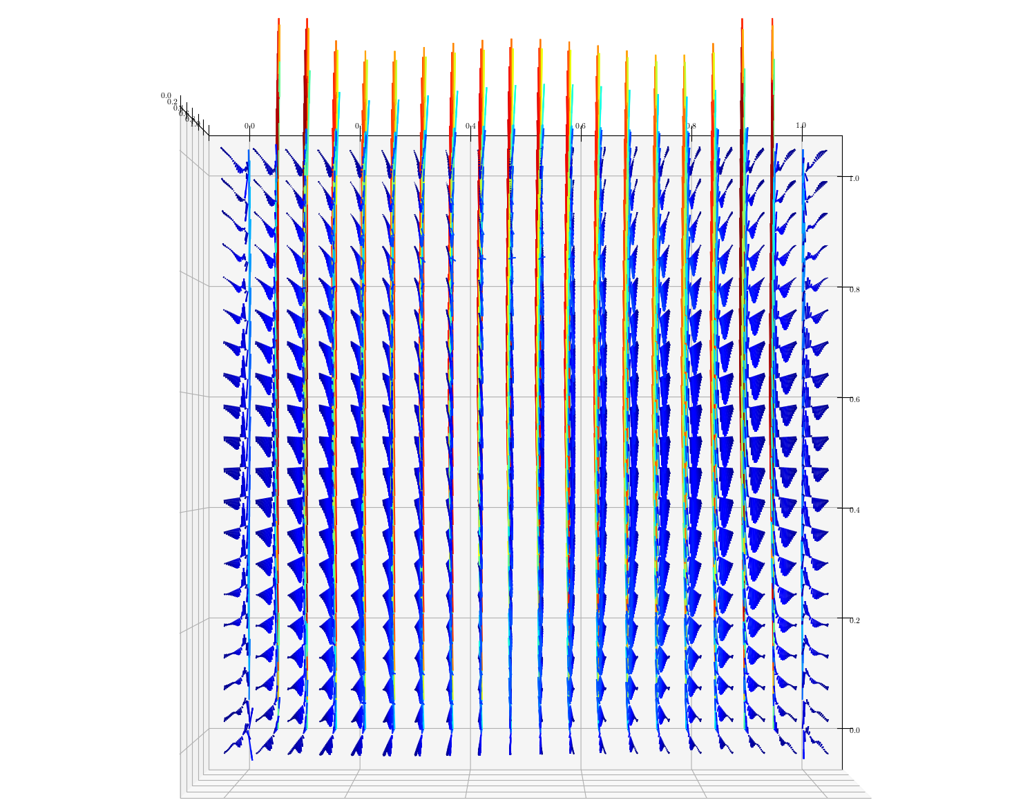
(f) view from z-axis

Figure 15: Numerical results of lid-driven cavity test case obtained with VPVnet method using $1000$ and $8000$ locally refine quadrature points in $\Omega$.

6 Discussion and conclusion

A deep neural network method is proposed and verified to approximate the solution of the Stokes’ equations. The method makes use of least square functionals based on the first-order VPV formulation (2) of the Stokes’ equations as loss functions. It has less regularity requirements on the solutions compared with other methods such as the methods based on the original form of the PDEs [40, 51]. Convergence and error estimates have been established for this method. We observed that smooth solutions of the Stokes’ equations can be well approximated by the VPVnet method using Resnet neural networks with a rather small number of neurons and hidden layers. Within a certain limit, a better precision can be obtained by using more hidden layers, more neurons and more quadrature points. Either smooth activation function, such as $Sin(x)$, $Tanh$, $Sigmoid$, etc can be employed and all of them can provide satisfying approximations. The method is divergence-free and pressure-robust.

We focus on the ability of the method for the approximation of Stokes’ equations with non-smooth/singular solutions, i.e. $u\notin H^{2}$ and $p\notin H^{1}$. For the velocity variable $\bm{u}\in H^{s}$, $2>s>1$ ($\in C^{0}$), the VPVnet methods can approximate it very well, which is in consistent with our theoretical analysis. As for the pressure variable $p\in H^{s-1}$, $2>s>1$ ($\notin C^{0}$), the approximation turn to be more difficult. Refinement can help to improve the precision, while more efforts is needed to reach a precision satisfying. The future work will be aimed at further investigation on this aspect. In the meantime, a variant of the proposed VPVnet method is under investigation, namely the VVGPnet method which is based on the first-order system of velocity/velocity gradient/pressure (VVGP) formulation [45] of the Stokes’ equations. The VVGP system also provides a $H^{1}$ least square functional and can be approximated similarly as the VPVnet method. The VVGPnet method is quite suitable for the approximation of the Stokes interface problems [60], which usually has jumps of the gradient of the velocity. The method will be detailed in a forthcoming paper dedicated for the interface problems.

The method presented here has already been extended to the incompressible Navier-Stokes Equations and will be discussed in a forthcoming paper.

References

- [1] S. Agmon, A. Douglis, L. Nirenberg. Estimates near the boundary for solutions of elliptic partial differential equations satisfying general boundary conditions II, Communications on pure and applied mathematics, 17(1), 35-92.
- [2] T. Arbogast, D. S. Brunson. A computational method for approximating a Darcy-Stokes system governing a vuggy porous medium. Computational Geosciences, 2007, 11(3):207-218.
- [3] A. G. Baydin, B. A. Pearlmutter, A. Radul, J. M. Siskind, Automatic differentiation in machine learning: a survey. Journal of Machine Learning Research, 18(1), 5595-5637, 2017.
- [4] C. Beck, M. Hutzenthaler, A. Jentzen, B. Kuckuck, An overview on deep learning-based approximation methods for partial differential equations. arXiv preprint :2012.12348, 2020.
- [5] A. Biswas, J. Tian, S. Ulusoy. Error Estimates for Deep Learning Methods in Fluid Dynamics. 2020, arXiv preprint arXiv:2008.02844.
- [6] P. B. Bochev, M. D. Gunzburger, Analysis of least squares finite element methods for the Stokes equations[J]. Mathematics of Computation, 1994, 63(208): 479-506.
- [7] P. B. Bochev, D. Gunzburger, Finite element methods of least-squares type. SIAM Review, 1998, 40:789-837.
- [8] O. Botella, R. Peyret. Benchmark spectral results on the lid-driven cavity flow. Computers & Fluids, 1998, 27(4): 421-433.
- [9] S. L. Brunton, B. R. Noack, P. Koumoutsakos, Machine learning for fluid mechanics, Annual Review of Fluid Mechanics, 2020, 52: 477-508.
- [10] Z. Cai, J. Chen, M. Liu, and X. Liu. Deep least-squares methods: An unsupervised learning-based numerical method for solving elliptic PDEs. Journal of Computational Physics, 2020, 420: 109707.
- [11] W. Cai, X. Li, L. Liu, A Phase Shift Deep Neural Network for High Frequency Approximation and Wave Problems. SIAM Journal on Scientific Computing, 42(5), A3285-A3312, 2020.
- [12] Z. Cai, Y. Wang. An error estimate for two-dimensional Stokes driven cavity flow. Mathematics of computation, 2009, 78(266): 771-787.
- [13] C. L. Chang, J. Bo-Nan, An error analysis of least-squares finite element method of velocity-pressure-vorticity formulation for Stokes problem. Computer methods in applied mechanics and engineering, 1990, 84(3), 247-255.
- [14] A. Chernov, C. Marcati, L. Mascotto, p-and hp-virtual elements for the Stokes equation. SAM Research Report, 2020.
- [15] R. Codina, O. Soto. Finite element solution of the Stokes problem with dominating Coriolis force. Computer Methods in Applied Mechanics and Engineering, 1997, 142(3-4):215-234.
- [16] J. M. Deang and M. D. Gunzburger. Issues related to least-squares finite element methods for the Stokes equations. SIAM Journal on Scientific Computing, 20(3), 878-906, 1998.
- [17] M. W. M. G. Dissanayake, N. Phan-Thien. Neural network based approximations for solving partial differential equations. Communications in Numerical Methods in Engineering, 10(3):195-201, 1994.
- [18] R. Duran, L. Gastaldi, A. Lombardi, Analysis of Finite Element Approximations of Stokes Equations with NonSmooth Data. SIAM Journal on Numerical Analysis, 2020, 58(6): 3309-3331.
- [19] W.-N. E, B. Yu, The Deep Ritz Method: A Deep Learning-Based Numerical Algorithm for Solving Variational Problems. Communications in Mathematics & Statistics, 2018, 6(1):1-12.
- [20] W.-N. E, Machine Learning and Computational Mathematics. Communications in Computational Physics, 2020, 28:1639-1670.
- [21] F. Gibou, D. Hyde, R. Fedkiw, Sharp interface approaches and deep learning techniques for multiphase flows. Journal of Computational Physics, 2019, 380: 442-463.
- [22] V. Girault and P.-A. Raviart, Finite Element Methods for Navier-Stokes Equations, Springer-Verlag, Berlin, 1986.
- [23] M. Gunzburger and J. Peterson, On conforming finite element methods for the inhomogeneous stationary Navier-Stokes equations, Numer. Math., 1983, 42,173-194.
- [24] C. He, X. Hu, L. Mu. A Mesh-free Method Using Piecewise Deep Neural Network for Elliptic Interface Problems. arXiv preprint arXiv:2005.04847, 2020.
- [25] K. He, X. Zhang, S. Ren, J. Sun, Deep residual learning for image recognition. In Proceedings of the IEEE conference on computer vision and pattern recognition, 2016, 770-778.
- [26] J. He, L. Li, J. Xu, and C Zheng, ReLU deep neural networks and linear finite elements[J]. arXiv preprint arXiv:1807.03973, 2018.
- [27] K. Hornik, Approximation capabilities of multilayer feedforward networks. Neural networks, 1991, 4(2): 251-257.
- [28] A. Iskhakov, N. Dinh, Physics-integrated machine learning: embedding a neural network in the Navier-Stokes equations. arXiv preprint arXiv:2008.10509, 2020.
- [29] A. Iskhakov, N. Dinh, Physics-integrated machine learning: embedding a neural network in the Navier-Stokes equations. Part II. arXiv preprint arXiv:2009.11213, 2020.
- [30] B.-N. Jiang, C. L. Chang, Least-squares finite elements for the Stokes problem[J]. Computer Methods in Applied Mechanics and Engineering, 1990, 78(3): 297-311.
- [31] B.-N. Jiang, A least-squares finite element method for incompressible Navier-Stokes problems[J]. International Journal for Numerical Methods in Fluids, 1992, 14(7): 843-859.
- [32] B.-N. Jiang, T. L. Lin, L. A. Povinelli, Large-scale computation of incompressible viscous flow by least-squares finite element method[J]. Computer Methods in Applied Mechanics and Engineering, 1994, 114(3-4): 213-231.
- [33] X. Jin, S. Cai, H. Li, G. E. Karniadakis, NSFnets (Navier-Stokes Flow nets): Physics-informed neural networks for the incompressible Navier-Stokes equations. arXiv preprint arXiv:2003.06496, 2020
- [34] E. Kharazmi, Z. Zhang, G. E. Karniadakis, Variational physics-informed neural networks for solving partial differential equations.
- [35] R. Khodayi-Mehr, M. Zavlanos, VarNet: Variational neural networks for the solution of partial differential equations, In Learning for Dynamics and Control, 2020, 298-307.
- [36] D. Kingma, J. Ba, Adam: A method for stochastic optimization, arXivpreprint arXiv:1412.6980, 2014.
- [37] I. E. Lagaris, A. Likas, D. I. Fotiadis, Artificial neural networks for solving ordinary and partial differential equations, IEEE Transactions on Neural Networks, 1998, 9(5): 987-1000.
- [38] I. E. Lagaris, A. C. Likas, D. G. Papageorgiou, Neural-network methods for boundary value problems with irregular boundaries, IEEE Transactions on Neural Networks , 2000, 11, 1041-1049.
- [39] H. C. Lee, Efficient computations for linear feedback control problems for target velocity matching of Navier-Stokes flows via POD and LSTM-ROM. Electronic Research Archive, 2021, 29(3): 2533.
- [40] J. Li, J. Yue, W. Zhang, W. Duan. The Deep Learning Galerkin Method for the General Stokes Equations. arXiv preprint arXiv:2009.11701, 2020.
- [41] R. Li, Z. Sun, F. Yang, Z. Yang, A finite element method by patch reconstruction for the Stokes problem using mixed formulations. Journal of Computational and Applied Mathematics, 2019, 353, 1-20.
- [42] Z. Li, N. Kovachki, K. Azizzadenesheli, B. Liu, K. Bhattacharya, A. Stuart, A. Anandkumar. Fourier neural operator for parametric partial differential equations. arXiv preprint arXiv:2010.08895, 2020.
- [43] Y. Liao, P. Ming, Deep Nitsche Method: Deep Ritz Method with Essential Boundary Conditions, Communications in Computational Physics, 2021, 29: 1365-1384.
- [44] D. C. Liu, J. Nocedal, On the limited memory BFGS method for large scale optimization, Mathematical programming, 1989, 45: 503-528.
- [45] K. Liu. Hybrid First-Order System Least-Squares Finite Element Methods With The Application To Stokes And Navier-Stokes Equations, Doctoral dissertation, University of Colorado at Boulder, 2012.
- [46] K. Liu, T. A. Manteuffel, S. F McCormick, J. W. Ruge, L. Tang. Hybrid first-order system least squares finite element methods with application to Stokes equations. SIAM Journal on Numerical Analysis, 2013, 51(4), 2214-2237.
- [47] S. Markidis. Physics-Informed Deep-Learning for Scientific Computing. arXiv preprint arXiv:2103.09655, 2021.
- [48] R. Ranade, C. Hill, J. Pathak, DiscretizationNet: A machine-learning based solver for Navier-Stokes equations using finite volume discretization. Computer Methods in Applied Mechanics and Engineering, 2021, 378: 113722.
- [49] K. S. McFall, J. R. Mahan, Artificial neural network method for solution of boundary value problems with exact satisfaction of arbitrary boundary conditions, IEEE Transactions on Neural Networks, 2009, 20, 1221-1233.
- [50] S. Mehrkanoon, J. A. K. Suykens, Learning solutions to partial differential equations using LS-SVM, Neurocomputing, 2015, 159: 105-116.
- [51] M. Raissi, P. Perdikaris, G. E. Karniadakis. Physics-informed neural networks: A deep learning framework for solving forward and inverse problems involving nonlinear partial differential equations, Journal of Computational Physics, 2019, 378: 686-707.
- [52] M. Raissi, A. Yazdani, G. E. Karniadakis, Hidden fluid mechanics: Learning velocity and pressure fields from flow visualizations, Science, 2020, 367(6481): 1026-1030.
- [53] C. Reisinger, Y. Zhang, Rectified deep neural networks overcome the curse of dimensionality for nonsmooth value functions in zero-sum games of nonlinear stiff systems. arXiv preprint arXiv:1903.06652, 2019.
- [54] H. Sheng, C. Yang. PFNN: A Penalty-Free Neural Network Method for Solving a Class of Second-Order Boundary-Value Problems on Complex Geometries, Journal of Computational Physics, 2021, 427:110085.
- [55] J. Sirignano, K. Spiliopoulos. DGM: A deep learning algorithm for solving partial differential equations. Journal of computational physics, 2018, 375, 1339-1364.
- [56] Y. Tang, X. Li. A meshless complex variable Galerkin boundary node method for potential and Stokes problems. Engineering Analysis with Boundary Elements, 2017, 83: 204-216.
- [57] N. Thuerey, K. Weißenow, L. Prantl, X. Hu, Deep learning methods for Reynolds-averaged Navier-Stokes simulations of airfoil flows, AIAA Journal, 2020, 58(1): 25-36.
- [58] R. Verfürth. A Review of a Posteriori Error Estimation and Adaptive Mesh-Refinement Techniques. Chichester-Stuttgart, Wiley-Teubner, 1996.
- [59] T. Vu-Huu, C. Le-Thanh, H. Nguyen-Xuan, M. Abdel-Wahab, An equal-order mixed polygonal finite element for two-dimensional incompressible Stokes flows. European Journal of Mechanics-B/Fluids, 2020, 79, 92-108.
- [60] B. Wang, B. C. Khoo, Hybridizable discontinuous Galerkin method (HDG) for Stokes interface flow. Journal of Computational Physics, 247, 262-278.
- [61] B. Wang, W. Z. Zhang, W. Cai, Multi-Scale Deep Neural Network (MscaleDNN) Methods for Oscillatory Stokes Flows in Complex Domains. Communications in Computational Physics, 2020, 28: 2139-2157.
- [62] C. L. Wight, J. Zhao, Solving Allen-Cahn and Cahn-Hilliard equations using the adaptive physics informed neural networks. arXiv preprint arXiv:2007.04542, 2020.
- [63] T. Xie, F. Cao, The errors of simultaneous approximation of multivariate functions by neural networks. Computers & Mathematics with Applications, 2011, 61(10), 3146-3152.
- [64] J. Xu The finite neuron method and convergence analysis. arXiv preprint arXiv:2010.01458, 2020.