Semiparametric Conditional Factor Models: Estimation and Inference

Abstract

This paper introduces a simple and tractable sieve estimation of semiparametric conditional factor models with latent factors. We establish large-$N$-asymptotic properties of the estimators without requiring large $T$. We also develop a simple bootstrap procedure for conducting inference about the conditional pricing errors as well as the shapes of the factor loading functions. These results enable us to estimate conditional factor structure of a large set of individual assets by utilizing arbitrary nonlinear functions of a number of characteristics without the need to pre-specify the factors, while allowing us to disentangle the characteristics’ role in capturing factor betas from alphas (i.e., undiversifiable risk from mispricing). We apply these methods to the cross-section of individual U.S. stock returns and find strong evidence of large nonzero pricing errors that combine to produce arbitrage portfolios with Sharpe ratios above 3. We also document a significant decline in apparent mispricing over time.

Keywords: Characteristics, managed portfolios, factor models, PCA, sieve estimation, conditional moments, nonparametric estimation, strong approximation

1 Introduction

Over the half-century that passed since publication of FamaMacBeth_RiskReturn_1973 financial economists have continued to grapple with their central question: whether asset returns are proportional, on average, to these assets’ exposures to systematic risk. The debate has centered on the role of asset characteristics that appear to be related to average returns, and whether this relationship represents “mispricing” or, instead, the characteristics’ role in capturing dynamically changing risk exposures. The challenge is that neither the nature of such systematic sources of risk nor the role of characteristics in capturing time-varying and asset-specific exposures to these sources of risk is known ex ante.

We consider the following semiparametric factor model

$$y_{it}=\alpha(z_{it})+\beta(z_{it})^{\prime}f_{t}+\varepsilon_{it},i=1,\ldots,N,t=1,\ldots,T,$$ (1)

where $f_{t}$ is a $K\times 1$ vector of unobserved factors, $\beta(\cdot)$ is a $K\times 1$ vector of unknown factor loading functions, $\alpha(\cdot)$ is an unknown intercept function, $\varepsilon_{it}$ is the idiosyncratic component that cannot be explained by the common component, and $y_{it}$ and $z_{it}$—an $M\times 1$ vector of covariates—are observed. Our main focus is on cross-sectional asset pricing, where $y_{it}$ are asset return realizations while $z_{it}$ are pre-specified asset characteristics (i.e. they are known at the beginning of period $t$). In this case (1) describes a conditional factor model, in the sense that it captures time-variation in asset return exposures to the common factors (i.e., $\beta(z_{it})$) as well as the pricing errors (i.e., $\alpha(z_{it})$), which are both functions of characteristics (i.e., $z_{it}$). As emphasized by Cochrane_Presidential_2011, this model is central to empirical asset pricing, since it potentially allows for distinguishing between “risk” and “mispricing” explanations of the role of characteristics in predicting asset returns. Pooling the information in a multitude of stock characteristics and summarizing the common variation using a small number of factors would amount to “taming the zoo” of factors that proliferate in empirical asset pricing. The challenge to doing so is threefold: first, the identities of the common factors $f_{t}$ are unknown since the factors are latent; second, the functional forms of the $alpha$ and $beta$ functions are also generally unknown; finally, the cross-sectional dimension $N$ is typically much larger than the sample time-series length $T$, which renders standard tools of factor analysis inapplicable, especially when conditional covariances are time-varying.

We introduce a simple and tractable estimation method to recover both the latent factors and the functional parameters of the model, as well as develop formal inference procedures. First, we develop an easy-to-compute estimator for $\alpha(\cdot)$, $\beta(\cdot)$ and $f_{t}$ based on a sieve approximation to the nonparametric functions $\alpha(\cdot)$ and $\beta(\cdot)$. The estimators can be easily obtained by first running the regression of $y_{it}$ on sieves of $z_{it}$ for each $t$ and then applying principal component analysis (PCA) to the estimated coefficient matrix. Throughout the paper, we refer to the two-step procedure as the regressed-PCA. The first step of our procedure is a cross-sectional regression (FamaMacBeth_RiskReturn_1973). Thus, in asset pricing settings the regressed-PCA boils down to applying PCA to a relatively small set of characteristic-managed portfolios constructed via the Fama-MacBeth regressions. Second, we establish large sample properties of the estimators including consistency, rate of convergence, and asymptotic normality under mild conditions. In particular, we establish a strong approximation for the distribution of the estimator of the large dimensional coefficient matrix in the sieve approximation of $\alpha(\cdot)$ and $\beta(\cdot)$. These asymptotic results have several attractive properties: (i) they do not require large $T$; (ii) they allow $z_{it}$ to vary over time in a potentially non-stationary manner; (iii) they are applicable to unbalanced panels (which is useful since individual securities have varying life spans). Third, we provide two consistent estimators for the number of factors $K$, which are also easy to compute. This enables us to conduct the regressed-PCA without specifying the number of factors a priori.

In asset pricing, testing the restriction that $\alpha(\cdot)$ is equal to zero for a given set of factors $f_{t}$ is central for evaluating and comparing factor models. We show that linear specifications of $\alpha(\cdot)$ and $\beta(\cdot)$ that are widely used in existing literature may adversely influence estimation of $f_{t}$ when the true underlying functional relationships are nonlinear. Therefore, along with the flexible nonparametric estimators we provide specification tests for the shape of $\alpha(\cdot)$ and $\beta(\cdot)$ functions. We develop a simple bootstrap inference procedure for testing significance of pricing error $\alpha(\cdot)$ as well as for linearity of $\alpha(\cdot)$ and $\beta(\cdot)$. First, we propose a weighted bootstrap procedure to approximate the distribution of the estimator of the large-dimensional coefficient matrix in the sieve approximation of $\alpha(\cdot)$ and $\beta(\cdot)$ as well as construct a Wald-type test for examining the significance of $\alpha(\cdot)$. The main challenge to developing a valid bootstrap is that the asymptotic distribution usually involves a rotational transformation matrix, which could be different under the bootstrap distribution, invalidating the procedure. In order to solve this problem we enforce the same factor estimator in the bootstrap samples as in the actual data. Second, we develop a likelihood ratio-type test for examining the linearity of $\alpha(\cdot)$ and $\beta(\cdot)$. Specifically, we construct the test statistic by comparing estimators under the null hypothesis and the alternative hypothesis. The novelty of our construction is that we use the unrestricted factor estimator from the alternative to obtain the estimators of $\alpha(\cdot)$ and $\beta(\cdot)$ under the null. This ensures the same rotational transformation matrix under the null and the alternative and thus the consistency of our test. Both of these tests also enjoy the aforementioned attractive features of our estimators: our Monte Carlo simulations show that the finite sample performance of our estimators and tests is satisfactory and encouraging for large $N$, even when $T$ is small.

We apply our new methodology to analyze the cross section of individual stock returns in the US market. We use the same data set as in Kellyetal_Characteristics_2019, which is the closest study to ours in terms of its empirical aims, although both our econometric approach and empirical findings are quite different. First, in contrast to Kellyetal_Characteristics_2019; Kellyetal_IPCA_2017, our method does not attempt maximize the “fit” of the factor model to asset returns in time-series and cross-section simultaneously. Rather, we extract factors that capture the most time-series comovement in returns, as postulated by the arbitrage pricing theory (e.g., Ross_APT_1976), and then attribute average asset returns to their conditional loadings with these factors (or to pricing errors). Second, we allow for $\alpha(\cdot)$ and $\beta(\cdot)$ functions to be non-linear. In fact, we are able to test–and reject–the validity of the linear specifications. Third, we are able to conduct rolling small sub-sample analyses to accommodate changing factor dynamics as our methods do not require large sample length $T$. Finally, we are able to consistently estimate the number of latent factors.

Our empirical findings reveal that only one latent factor is detected by the formal tests when we consider linear dependence of $alpha$ and $beta$ functions on characteristics, and two factors when we allow for nonlinearity–this is also in contrast to Kellyetal_Characteristics_2019, who advocate a five-factor model. Still, our tests reject the risk-based model, since the pricing errors associated with many characteristics are statistically different from zero. Their economic magnitudes are also substantial, as we are able to construct pure-$alpha$ portfolios with annualized Sharpe ratios typically above 3 (as is common in the literature, we refer to these as “arbitrage” portfolios, even though their returns are far from riskless). These Sharpe ratios tend to rise with the number of factors (we consider up to ten), indicating that adding factors does not improve the asset pricing properties of the model, even though it might help capture more time-series variation in returns. This result provides strong empirical evidence that the characteristics contain information about both risk exposures and mispricing. In addition, the nonlinear models often produce more reasonable estimated relationships between the risk exposures and characteristics than the linear model. For instance, the estimates from our nonlinear models show that firms with higher book-to-market ratios bear more systematic risk and hence have higher expected returns, whereas the estimates from the linear model often give the opposite result. Nevertheless, the additional flexibility provided by the nonparametric estimation of factor loadings does not result in an improved asset pricing performance of the factor models, yielding arbitrage portfolio Sharpe ratios that are as high or even higher than in the linear case, often exceeding 4. However, we also document the significant decline of pricing errors and arbitrage portfolio Sharpe ratios in the more recent years, in particular since 2000, potentially consistent with growth in quantitative investing that reduces mispricing by exploiting characteristic-related anomalies (e.g. as suggested by McLeanPontiff_DoesAcademic_2016 or Greenetal_Characteristics_2017). We also show that both in-sample and out-of-sample goodness of fits for all factor models declines from 1970 until roughly 2000 but increases thereafter, which is consistent with the findings in Campbell2001have and Campbell2022idiosyncratic on the time-variation in the amount of idiosyncratic volatility in the U.S. stock market.

Our paper relates to several strands of literature. Several studies estimate models similar to (1) under the assumption that $z_{it}$ are time-invariant, at least over subsamples. ConnorLinton_Semparametric_2007 and Connoretal_EfficientFFFactor_2012 develop estimation procedures based on kernel smoothing for the case with $\alpha(\cdot)=0$ and $\beta(\cdot)$ being univariate functions. Fanetal_ProjectedPCA_2016 consider a sieve estimation which facilitates global inference, and propose a projected-PCA approach for the case with $\alpha(\cdot)=0$. Kimetal_Arbitrage_2019 extend the projected-PCA to allow for nonzero $\alpha(\cdot)$ and use it to construct an arbitrage portfolio, while LiGeLinton_Dynamic_2020 develop a test of $\alpha(\cdot)=0$. Fanetal_StructuralDeep_2022 extend the projected-PCA by using deep neural networks to approximate $\alpha(\cdot)$ and $\beta(\cdot)$, and propose a local version of projected-PCA that relies on smooth behavior of $z_{it}$ over time. We contribute to this literature by introducing a robust sieve estimation that allows $z_{it}$ to vary over time and developing global inference for $\alpha(\cdot)$ and $\beta(\cdot)$. Despite some similarities, our regressed-PCA is genetically different from the projected-PCA. The regression in the former serves to extract $z_{it}$ from the common component for a consistent estimation, whereas the projection in the latter serves to remove the noise part of the factor loadings for a more efficient estimation. Therefore, the projected-PCA may fail to obtain consistent estimators when $z_{it}$ are time-varying. In contrast, our regressed-PCA is consistent even when $z_{it}$ are nonstationary over time.

Our study also contributes to the literature on time-varying factor models. Mottaetal_LocallyStationary_2011 and SuWang_TimeVarying_2017 consider the time-varying factor model with factor loadings being smooth functions of $t/T$ and propose local versions of PCA based on kernel smoothing. PelgerXiong_State-varying_2019 assume that factor loadings are smooth functions of state variables and study a similar estimation procedure. GagliardiniMa_Extracting_2019 study a time-varying factor model with no arbitrage and extract local factors from conditional variance matrices. However, none of them are directly suitable for testing asset pricing models, since they all impose $\alpha(\cdot)=0$. Many empirical findings suggest that characteristics contain information about both pricing errors and risk exposures, which can be distinguished in our approach. There are numerous studies of conditional models with observed factors. For example, Gagliardinietal_Timevarying_2016 specify factor loadings as linear functions of both time-varying characteristics and state variables in a model with $\alpha(\cdot)=0$; Gagliardinietal_EstimationConditionalFactor_2019 provide a comprehensive review.

The literature on the cross section of asset returns is vast; here we focus on multi-factor models motivated by the arbitrage pricing theory of Ross_APT_1976 and its generalizations (ChamberlainRothschild_FactorStuctures_1982; ConnorKorajczyk_Performance_1986; ConnorKorajczyk_RiskReturn_1988; Reisman/IAPT:1992). Empirical analysis that exploits the ability of stock characteristics to predict asset returns typically follows either the portfolio-sorting approach (FamaFrench_Commonrisk_1993; DanielTitman_Characteristics_1997; FamaFrench_FiveFactor_2015) or the characteristic-based approach (RosenbergMcKibben_ThePrediction_1973; Jacobs/Levy:88; Lewellen_Crosssection_2015; Greenetal_Characteristics_2017; Freybergeretal_Dissecting_2017; Kirby_FirmChar_2020; GiglioXiu_Asset_2019). The importance of nonlinearity is highlighted by several empirical studies (Connoretal_EfficientFFFactor_2012; Kirby_FirmChar_2020), and has also been addressed by machine learning methods in recent studies (Guetal_Autoencoder_2021; Chenetal_DeepLearning_2020).

The central issue with both of these approaches is that they are unable to distinguish between the two roles played by characteristics: capturing time-varying risk exposures and representing mispricing. We complement the literature by introducing a semiparametric time-varying characteristic-based factor model that provides a simple, tractable and robust method for estimation and inference. This new methodology enables us to estimate conditional (dynamic) behavior of a large set of individual assets from a number of characteristics exhibiting nonlinearity without the need to pre-specify factors, while allowing us to disentangle the risk and mispricing explanations, as least from the standpoint of arbitrage-based models.

The remainder of the paper is organized as follows. Section 2 introduces the estimation method—the regressed-PCA. Section 3 establishes large sample properties of the estimators, including consistency, rate of convergence, and asymptotic distribution. Section 4 introduces a weighted bootstrap and develops two tests. Section 5 provides two consistent estimators of the number of factors. Section 6 applies our new methodology to analyze the cross section of individual stock returns in the US market. Section 7 briefly concludes. Appendix A collects assumptions, while Appendix B provides proofs of the main results. The Online Appendix presents auxiliary results, simulation results, additional empirical results, and technical lemmas.

2 Estimation Method

In this section we introduce the approach to estimating a latent factor model that we term regressed principal component analysis or regressed-PCA.

We first illustrate the idea behind our regressed-PCA method by assuming that $\alpha(\cdot)$ is null and $\beta(\cdot)$ is linear: $\alpha(\cdot)=0$ and $\beta(z_{it})=\Gamma^{\prime}z_{it}$ for some $M\times K$ matrix $\Gamma$. Let $Y_{t}\equiv(y_{1t},\ldots,y_{Nt})^{\prime}$, $Z_{t}\equiv(z_{1t},\ldots,z_{Nt})^{\prime}$, and $\varepsilon_{t}\equiv(\varepsilon_{1t},\ldots,\varepsilon_{Nt})^{\prime}$. Then we may write (1) in a matrix form

$$Y_{t}=Z_{t}\Gamma f_{t}+\varepsilon_{t}.$$ (2)

The main challenge in applying standard PCA to estimating $\Gamma$ and $f_{t}$ is the presence of $Z_{t}$ in the first term on the right-hand side of (2). In order to circumvent this problem, we first regress $Y_{t}$ on $Z_{t}$. Thus, we obtain

$$(Z_{t}^{\prime}Z_{t})^{-1}Z_{t}^{\prime}Y_{t}=\Gamma f_{t}+(Z_{t}^{\prime}Z_{t})^{-1}Z_{t}^{\prime}\varepsilon_{t}.$$ (3)

Heuristically, variation in the common component $Z_{t}\Gamma f_{t}$ over $t$ comes from two sources, $Z_{t}$ and $f_{t}$, and regressing $Y_{t}$ on $Z_{t}$ helps isolate them by extracting $Z_{t}$ from the common component. Given the factor structure on the right-hand side of (3), we can apply the standard PCA to $\{(Z_{t}^{\prime}Z_{t})^{-1}Z_{t}^{\prime}Y_{t}\}_{t\leq T}$ in order to obtain estimators of $\Gamma$ and $f_{t}$.

The model in (2) can be alternatively viewed as a panel data model with time-varying slope coefficients $\Gamma f_{t}$, which exhibit a factor structure. Essentially, the regressed-PCA first estimates the time-varying slope coefficients by period-by-period cross-sectional regressions, and then exploits the factor structure by using PCA.

2.1 Regressed-PCA Estimation

Now we consider the general case with nonzero $\alpha(\cdot)$ and show how to estimate $\alpha(\cdot)$ and $\beta(\cdot)=(\beta_{1}(\cdot),\ldots,\beta_{K}(\cdot))^{\prime}$ nonparametrically. To estimate $\alpha(\cdot)$ and $\beta_{k}(\cdot)$ without falling prey to the curse of dimensionality when $z_{it}$ is multivariate, we assume $\alpha(\cdot)$ and $\beta_{k}(\cdot)$ are separable. Specifically, we assume that there are $\{\alpha_{m}(\cdot)\}_{m\leq M}$ and $\{\beta_{km}(\cdot)\}_{m\leq M}$ such that

$$\alpha(z_{it})=\sum_{m=1}^{M}\alpha_{m}(z_{it,m})\text{ and }\beta_{k}(z_{it})=\sum_{m=1}^{M}\beta_{km}(z_{it,m}),$$ (4)

where $z_{it,m}$ is the $m$th entry of $z_{it}$. We adopt the sieve method to estimate $\alpha_{m}(\cdot)$ and $\beta_{km}(\cdot)$. Let $\{\phi_{j}(\cdot)\}_{j\geq 1}$ be a set of basis functions (e.g., B-spline, Fourier series, polynomials), which spans a dense linear space of the functional space for $\alpha_{m}(\cdot)$ and $\beta_{km}(\cdot)$. Then we may write

$$\alpha_{m}(z_{it,m}) =\sum_{j=1}^{J}a_{m,j}\phi_{j}(z_{it,m})+r_{m,J}(z_{it,m}),$$ (5)

$$\beta_{km}(z_{it,m}) =\sum_{j=1}^{J}b_{km,j}\phi_{j}(z_{it,m})+\delta_{km,J}(z_{it,m}).$$ (6)

Here, $\{a_{m,j}\}_{j\leq J}$ and $\{b_{km,j}\}_{j\leq J}$ are the sieve coefficients; $r_{m,J}(\cdot)$ and $\delta_{km,J}(\cdot)$ are “remaining functions” representing the approximation errors; $J$ denotes the sieve size. The basic assumption for the sieve method is that $\sup_{z}|r_{m,J}(z)|\to 0$ and $\sup_{z}|\delta_{km,J}(z)|\to 0$ as $J\to\infty$. Let $\bar{\phi}(z_{it,m})\equiv(\phi_{1}(z_{it,m}),\ldots,\phi_{J}(z_{it,m}))^{\prime}$, ${\phi}(z_{it})\equiv(\bar{\phi}(z_{it,1})^{\prime},\ldots,\bar{\phi}(z_{it,M})^{\prime})^{\prime}$, $a\equiv(a_{1,1},\ldots,a_{1,J},\ldots,a_{M,1},\ldots,a_{M,J})^{\prime}$ which is a $JM\times 1$ vector of the sieve coefficients, $b_{k}\equiv(b_{k1,1},\ldots,b_{k1,J},\ldots,b_{kM,1},\ldots,b_{kM,J})^{\prime}$, and $B\equiv(b_{1},\cdots,b_{K})$ which is a $JM\times K$ matrix of the sieve coefficients. Let $r(z_{it})\equiv\sum_{m=1}^{M}r_{m,J}(z_{it,m})$ and $\delta(z_{it})\equiv(\sum_{m=1}^{M}\delta_{1m,J}(z_{it,m}),\ldots,\sum_{m=1}^{M}\delta_{Km,J}(z_{it,m}))^{\prime}$. Then

$$\alpha(z_{it})=a^{\prime}\phi(z_{it})+r(z_{it})\text{ and }\beta(z_{it})=B^{\prime}\phi(z_{it})+\delta(z_{it}).$$ (7)

Thus, $\alpha(z_{it})$ and $\beta(z_{it})$ can be well approximated by $a^{\prime}\phi(z_{it})$ and $B^{\prime}\phi(z_{it})$ under the basic sieve assumption, and estimating $\alpha(\cdot)$ and $\beta(\cdot)$ reduces to estimating $a$ and $B$.

We now introduce the estimation of $a$, $B$ and $f_{t}$ based on the above sieve approximation in (7) by adapting the regressed-PCA.Let $\Phi(Z_{t})\equiv({\phi}(z_{1t}),\ldots,{\phi}(z_{Nt}))^{\prime}$, $R(Z_{t})\equiv(r(z_{1t}),\ldots,r(z_{Nt}))^{\prime}$ and $\Delta(Z_{t})\equiv(\delta(z_{1t}),\ldots,\delta(z_{Nt}))^{\prime}$. Using the sieve approximation in (7), we may write (1) in a matrix form

$$Y_{t}=\Phi(Z_{t})a+\Phi(Z_{t})Bf_{t}+R(Z_{t})+\Delta(Z_{t})f_{t}+\varepsilon_{t}.$$ (8)

Under the basic sieve assumption, the term “$R(Z_{t})+\Delta(Z_{t})f_{t}$” is negligible, so the main challenge in applying standard PCA to estimating $a$, $B$ and $f_{t}$ is the presence of $\Phi(Z_{t})$ in the first two terms on the right-hand side of (8). To solve this problem we regress $Y_{t}$ on $\Phi(Z_{t})$ to obtain

$$\tilde{Y}_{t}=a+Bf_{t}+(\Phi(Z_{t})^{\prime}\Phi(Z_{t}))^{-1}\Phi(Z_{t})^{\prime}(R(Z_{t})+{\Delta}(Z_{t})f_{t}+{\varepsilon}_{t}),$$ (9)

where $\tilde{Y}_{t}=(\Phi(Z_{t})^{\prime}\Phi(Z_{t}))^{-1}\Phi(Z_{t})^{\prime}Y_{t}$. Thus, we estimate $a$, $B$ and $f_{t}$ as follows. First, since $\tilde{Y}_{t}\approx a+Bf_{t}$, we can remove $a$ by subtracting $\bar{\tilde{Y}}=\sum_{t=1}^{T}\tilde{Y}_{t}/T$ from $\tilde{Y}_{t}$ and estimate $B$ by applying the standard PCA to the demeaned $\{\tilde{Y}_{t}-\bar{\tilde{Y}}\}_{t\leq T}$. Second, for identification of $a$ (and thus $\alpha(\cdot)$), we assume $a^{\prime}B=0$. Since $\bar{\tilde{Y}}\approx a+B\bar{f}$ where $\bar{f}=\sum_{t=1}^{T}f_{t}/T$, we can estimate $a$ according to $a\approx[I_{JM}-B(B^{\prime}B)^{-1}B]\bar{\tilde{Y}}$. Third, we can estimate $f_{t}$ according to $f_{t}\approx(B^{\prime}B)^{-1}B^{\prime}\tilde{Y}_{t}$.

The estimators of $a$, $B$, $\alpha(\cdot)$, $\beta(\cdot)$ and $F=(f_{1},\ldots,f_{T})^{\prime}$ are formally defined as follows. Denote the estimators by $\hat{a}$, $\hat{B}$, $\hat{\alpha}(\cdot)$, $\hat{\beta}(\cdot)$ and $\hat{F}$. Let $M_{T}\equiv I_{T}-1_{T}1_{T}^{\prime}/T$, where $1_{T}$ denotes a $T\times 1$ vector of ones. We use the following normalization: $B^{\prime}B=I_{K}$ and $F^{\prime}M_{T}F/T$ being diagonal with diagonal entries in descending order. Let $\tilde{Y}\equiv(\tilde{Y}_{1},\ldots,\tilde{Y}_{T})$. Then the columns of $\hat{B}$ are the eigenvectors corresponding to the first $K$ largest eigenvalues of the $JM\times JM$ matrix $\tilde{Y}M_{T}\tilde{Y}^{\prime}/T$, $\hat{a}=(I_{JM}-\hat{B}\hat{B}^{\prime})\bar{\tilde{Y}}$, and

$$\hat{\alpha}(z)=\hat{a}^{\prime}\phi(z),\hat{\beta}(z)=\hat{B}^{\prime}\phi(z)\text{ and }\hat{F}=(\hat{f}_{1},\ldots,\hat{f}_{T})^{\prime}=\tilde{Y}^{\prime}\hat{B}.$$ (10)

Here, we assume that $K$—the number of factors—is known, and conduct asymptotic analysis and develop inference method in Sections 3 and 4. In Section 5, we develop two consistent estimators of $K$, so all the results carry over to the unknown $K$ case using a conditioning argument.

2.2 Key Properties

Our regressed-PCA estimation enjoys several desirable properties, and is also easy to implement. First of all, as elucidated in Section 3.1, it accommodates time-varying characteristics and does not require large $T$. Thus, it allows us to examine the changing relationship between risk and return via both full-sample and sub-sample analyses.

Our estimation procedure is also applicable for unbalanced panels, which is especially pertinent to cross-sectional asset pricing applications. The key step of regressed-PCA is to obtain $\tilde{Y}_{t}$. We may write $\tilde{Y}_{t}=[\sum_{i=1}^{N}\phi(z_{it})\phi(z_{it})^{\prime}]^{-1}\sum_{i=1}^{N}\phi(z_{it})y_{it}$. In the case of an unbalanced panel, we may obtain $\tilde{Y}_{t}$ by taking the two sums over $i$’s, for which both $z_{it}$ and $y_{it}$ are observed in time period $t$. This is equivalent to replacing missing data with zeros and proceeding as balanced panels. The asymptotic results established in the following sections continue to hold as $\min_{t\leq T}N_{t}\to\infty$, where $N_{t}$ is the sample size in time period $t$.

Our estimation procedure continues to work when pricing errors and risk exposures are not fully captured by $z_{it}$. Let $e_{\alpha,it}$ and $e_{\beta,it}$ error terms in the pricing errors and the risk exposures, which are not explained by $z_{it}$ (i.e.,, orthogonal to $z_{it}$). It follows that

$$y_{it}=[\alpha(z_{it})+e_{\alpha,it}]+[\beta(z_{it})+e_{\beta,it}]^{\prime}f_{t}+\varepsilon_{it}=\alpha(z_{it})+\beta(z_{it})^{\prime}f_{t}+\varepsilon^{\ast}_{it},$$

where $\varepsilon^{\ast}_{it}=\varepsilon_{it}+e_{\alpha,it}+e_{\beta,it}^{\prime}f_{t}$. Notice that we are not interested in estimating $e_{\alpha,it}$ and $e_{\beta,it}$. Thus, the asymptotic properties that we derive continue if we replace $\varepsilon_{it}$ in (1) by $\varepsilon^{\ast}_{it}$.

Moreover, efficiency of estimation could potentially be improved by using generalized least squares in the first step estimation. The asymptotic results that we derive continue to hold if we replace $\Phi(Z_{t})$ and $\varepsilon_{t}$ with the corresponding transformations $V_{t}^{-1/2}\Phi(Z_{t})$ and $V_{t}^{-1/2}\varepsilon_{t}$, where $V_{t}$ is the conditional covariance matrix of $Y_{t}$ for each $t$.

2.3 Comparing Methods

How does our regressed-PCA compare with existing methods that have been proposed in the literature?

First, the projected-PCA of Fanetal_ProjectedPCA_2016 applies the standard PCA to the projected data—$\{\Phi(Z_{t})(\Phi(Z_{t})^{\prime}\Phi(Z_{t}))^{-1}\Phi(Z_{t})^{\prime}Y_{t}\}_{t\leq T}$. The regression in the regressed-PCA is designed to extract $Z_{t}$ from the common component for a consistent estimation, whereas the projection in the projected-PCA is designed to remove the noise in the factor loadings for a more efficient estimation. Therefore, the projected-PCA may fail to provide consistent estimates when $Z_{t}$ is time-varying. Indeed, as discussed by Fanetal_ProjectedPCASupp_2016 and further investigated by Fanetal_StructuralDeep_2022 and Chengetal_UniformPredictive_2020, one may need to impose certain smoothness conditions on how $Z_{t}$ varies with $t$ to ensure the consistency of the projected-PCA. Our regressed-PCA does not require such conditions. Moreover, the projected-PCA may require that certain observations be dropped in order to obtain a balanced panel, while regressed-PCA is applicable to unbalanced panels.

Second, consider the least squares estimation approach (Parketal_FactorDynamics_2009), which is at the core of the instrumented PCA (IPCA) of Kellyetal_Characteristics_2019. The least squares estimation problem is nonconvex and thus cannot be solved explicitly; Parketal_FactorDynamics_2009 develop a numerical algorithm to find the estimators, while Kellyetal_Characteristics_2019 propose an alternating least squares procedure. However, both methods may require a good choice of initial values as convergence to the correct solution is not assured and their asymptotic properties are not well-understood. Lastly, while IPCA implicitly relies on a long time-series of returns, regressed-PCA does not require a large $T$, which allows for sub-sample analyses as well as capturing potential time-variation in the coefficients ($a$ and $B$).

Overall, in addition to the asymptotic properties that we derive, our estimators can always be explicitly solved for, and their computation is easy since it involves only least-squares regression and PCA.

2.4 Asset Pricing Interpretation

In a typical asset pricing application $y_{it}$ would be realized returns on asset $i$ at the end of period $t$, while $z_{it,m}$ would represent an $m$’th attribute/characteristic of asset $i$ that is known a the beginning of period $t$ (or, alternatively, at the “end” of period $t-1$). The regressed-PCA first estimates the time-varying slope coefficients by period-by-period cross-sectional regressions of returns on (functions of) asset characteristics, and then exploits the factor structure by using PCA. The period-by-period cross-sectional regressions are known as Fama-MacBeth regressions (FamaMacBeth_RiskReturn_1973), which help transform the large unbalanced panel of noisy individual asset returns into a low-dimensional balanced panel of assets that are largely free of idiosyncratic noise, $\tilde{Y}_{t}$. In asset pricing applications, $\tilde{Y}_{t}$ can be interpreted as the time $t$ realization of returns on a set of $JM$ managed portfolios, sometimes referred to as “characteristic pure plays” or “cross-sectional factors” (e.g. as in Backetal_PurePlays_2015 or FamaFrench_CSTS_2020).

In particular, if the sieve basis ($\Phi(Z_{t})$) includes a constant term (e.g. as the first element in $\Phi(Z_{t})$), and is also standardized to have a zero mean in each cross-section, then intercept in Fama-MacBeth regressions (the first element in $\tilde{Y}_{t}$) is a “level” return, which is the equal-weighted average excess return across all individual assets with weights that sum up to unity (sometimes referred to as a “naively diversified” or $1/N$ portfolio). As shown by Fama_76, the period-by-period slope coefficients corresponding to the time-varying characteristics are excess returns on zero-cost portfolios with weights on individual assets that set the weighted average value of the relevant characteristic to one and that of all the remaining characteristics bases to zero, as long as the right-hand side variables are suitably normalized (Kirby_FirmChar_2020 discusses other attractive properties of these portfolios). In our setting, the $\ell$th entry of $\tilde{Y}_{t}$ is a portfolio return (i.e. a weighted average of all test asset returns) with weights determined by the $\ell$th row of $(\Phi(Z_{t})^{\prime}\Phi(Z_{t}))^{-1}\Phi(Z_{t})^{\prime}$, which is a standardized version of $\Phi(Z_{t})$. If $\Phi(Z_{t})^{\prime}\Phi(Z_{t})$ is diagonal, the portfolios are normalized by the second moment of $\Phi(Z_{t})$.

3 Asymptotic Analysis

In this section we establish consistency of our estimators and provide their asymptotic distributions. We begin by defining some notation that is used throughout the paper. For a symmetric matrix $A$, we denote its $k$th largest eigenvalue by $\lambda_{k}(A)$, and its smallest and largest eigenvalues by $\lambda_{\min}(A)$ and $\lambda_{\max}(A)$. For a matrix $A$, we denote its operator norm by $\|A\|_{2}$, its Frobenius norm by $\|A\|_{F}$, and its vectorization by $\mathrm{vec}(A)$. The Euclidian norm of a column vector $x$ is denoted $\|x\|$. For matrices $A$ and $B$, we use $A\otimes B$ to denote their Kronecker product.

3.1 Consistency and Rate of Convergence

Prior to presenting formal theorems, we return to (2) to quickly illustrate why large $T$ is not required and $Z_{t}$ are allowed to be nonstationary over $t$ in our asymptotic analysis. Assume $T\geq K+1$ and $M\geq K$. Since the columns of $\hat{B}$ and $\Gamma$ are the eigenvectors of $\tilde{Y}M_{T}\tilde{Y}^{\prime}$ and $\Gamma F^{\prime}M_{T}F\Gamma^{\prime}$ corresponding to the first $K$ largest eigenvalues, by the matrix perturbation theorem (see, for example, Yuetal_Useful_2014), to establish the consistency of $\hat{B}$ to $\Gamma$ (up to a rotational transformation) it suffices to show

$$\|\tilde{Y}M_{T}-\Gamma F^{\prime}M_{T}\|_{F}=o_{p}(1)\text{ as }N\to\infty.$$ (11)

Since $\tilde{Y}=\Gamma F^{\prime}+((Z_{1}^{\prime}Z_{1})^{-1}Z_{1}^{\prime}\varepsilon_{1},\ldots,(Z_{T}^{\prime}Z_{T})^{-1}Z_{T}^{\prime}\varepsilon_{T})$, (11) reduces to

$$\|((Z_{1}^{\prime}Z_{1})^{-1}Z_{1}^{\prime}\varepsilon_{1},\ldots,(Z_{T}^{\prime}Z_{T})^{-1}Z_{T}^{\prime}\varepsilon_{T})M_{T}\|_{F}=o_{p}(1)\text{ as }N\to\infty.$$ (12)

When $T$ is fixed, (12) is equivalent to $(Z_{t}^{\prime}Z_{t})^{-1}Z_{t}^{\prime}\varepsilon_{t}=o_{p}(1)$ for each $t$. Thus, we only need regularity conditions on $Z_{t}$ and $\varepsilon_{t}$ for each $t$ in order to apply the law of large numbers. This implies that $Z_{t}$ can vary over $t$ in a non-stationary manner.

Let $H\equiv(F^{\prime}M_{T}\hat{F})(\hat{F}^{\prime}M_{T}\hat{F})^{-1}$, which is a rotational transformation matrix that determines the convergence limit of $\hat{B}$, $\hat{F}$ and $\hat{\beta}(\cdot)$. Let $\xi_{J}\equiv\sup_{z}\|\bar{\phi}(z)\|$, which is $O(\sqrt{J})$ for B-spline and Fourier series and $O(J)$ for polynomials (see, for example, BelloniChernozhukovChetverikovKato_SeriesEstimator_2015). The first theoretical result of the paper is given as follows. We collect all assumptions with discussions in Appendix A.

Theorem 3.1.

Suppose Assumptions A.1-A.5 hold. Let $\hat{a}$, $\hat{B},\hat{F}$, $\hat{\alpha}(\cdot)$ and $\hat{\beta}(\cdot)$ be given in (10). Assume (i) $N\to\infty$; (ii) $T\to\infty$ or $T\geq K+1$ is finite; (iii) $J\to\infty$ with $J^{2}\xi^{2}_{J}\log J=o(N)$. Then

$$\|\hat{a}-a\|^{2} =O_{p}\left(\frac{1}{J^{2\kappa}}+\frac{J}{N^{2}}+\frac{{J}}{{NT}}\right),$$

$$\|\hat{B}-BH\|^{2}_{F} =O_{p}\left(\frac{1}{J^{2\kappa}}+\frac{J}{N^{2}}+\frac{{J}}{{NT}}\right),$$

$$\frac{1}{T}\|\hat{F}-F(H^{\prime})^{-1}\|_{F}^{2} =O_{p}\left(\frac{1}{J^{2\kappa}}+\frac{1}{{N}}\right),$$

$$\sup_{z}|\hat{\alpha}(z)-\alpha(z)|^{2} =O_{p}\left(\frac{1}{J^{2\kappa-1}}+\frac{J^{2}}{N^{2}}+\frac{{J^{2}}}{{NT}}\right)\max_{j\leq J}\sup_{z}|\phi_{j}(z)|^{2},$$

$$\sup_{z}\|\hat{\beta}(z)-H^{\prime}\beta(z)\|^{2} =O_{p}\left(\frac{1}{J^{2\kappa-1}}+\frac{J^{2}}{N^{2}}+\frac{{J^{2}}}{{NT}}\right)\max_{j\leq J}\sup_{z}|\phi_{j}(z)|^{2}.$$

We discuss two important findings. First, Theorem 3.1 implies that $a$ and $\alpha(\cdot)$ can be consistently estimated by $\hat{a}$ and $\hat{\alpha}(\cdot)$, and $B$, $F$ and $\beta(\cdot)$ can be consistently estimated by $\hat{B}$, $\hat{F}$ and $\hat{\beta}(\cdot)$ up to a rotational transformation under either large $N$ with fixed $T$ or large $N$ and large $T$. In particular, the consistency of $\hat{F}$ requires $J\to\infty$. This is because a large sieve approximation error of $\alpha(\cdot)$ and $\beta(\cdot)$ may cause inconsistent estimation of $F$. To quickly see this, let us look at the following simple linear models

$$Y_{t} =W_{t}\Pi+Z_{t}\Gamma f_{t}+\varepsilon_{t},$$ (13)

$$Y_{t} =(Z_{t}\Gamma+W_{t}\Pi)f_{t}+\varepsilon_{t},$$ (14)

where $Z_{t}$ and $W_{t}$ are $N\times 1$ vectors, $f_{t}$ is a scalar factor, and $\varepsilon_{t}$ is independent of $Z_{t}$ and $W_{t}$. Let us further assume $\Pi=\Gamma$ and $W_{t}=Z_{t}g_{t}+v_{t}$, where $g_{t}$ is a scalar coefficient, and $v_{t}$ is independent of $Z_{t}$. Then (13) and (14) can be rewritten as

$$Y_{t} =Z_{t}\Gamma f_{t}^{\star}+\varepsilon^{\star}_{t},$$ (15)

$$Y_{t} =Z_{t}\Gamma f_{t}^{\star\star}+\varepsilon^{\star\star}_{t},$$ (16)

where $f_{t}^{\star}=f_{t}+g_{t}$, $\varepsilon^{\star}_{t}=v_{t}\Gamma+\varepsilon_{t}$, $f_{t}^{\star\star}=f_{t}(1+g_{t})$, and $\varepsilon^{\star\star}_{t}=v_{t}\Gamma f_{t}+\varepsilon_{t}$. Thus, if only $Z_{t}$ is used for estimating (13) (i.e., the sieve approximation error of $\alpha(\cdot)$ is large), then $\hat{F}$ can consistently estimates $F^{\star}=(f_{1}^{\star},\ldots,f_{T}^{\star})^{\prime}$ up to a scalar; if only $Z_{t}$ is used for estimating (14) (i.e., the sieve approximation error of $\beta(\cdot)$ is large), then $\hat{F}$ can consistently estimate $F^{\star\star}=(f_{1}^{\star\star},\ldots,f_{T}^{\star\star})^{\prime}$ up to a scalar. In both cases, $\hat{F}$ fails to consistently estimate the space spanned by $F$, unless $g_{t}$ is proportional to $f_{t}$ in the former case and is not changing over $t$ in the latter case. The finding also suggests that misspefication of $\alpha(\cdot)$ and $\beta(\cdot)$ may cause inconsistent estimation of $F$, thus motivates us to develop a specification test for $\alpha(\cdot)$ and $\beta(\cdot)$ in Section 4.2.

Second, Theorem 3.1 provides a fast convergence rate of $\hat{a}$, $\hat{B}$ and $\hat{F}$. For example, when $T=O(N)$, $\hat{a}$ and $\hat{B}$ attains the optimal rate $O_{p}(J^{-2\kappa}+J/(NT))$, which is the fastest rate that one can obtain when $F$ were known. Assume $J^{-2\kappa}N=O(1)$, which can be satisfied for sufficiently large $\kappa$ under the restriction $J^{2}\xi^{2}_{J}\log J=o(N)$. Then $\hat{F}$ attains the optimal rate $O_{p}(1/N)$, which is the fastest rate that one can obtain when $\alpha(\cdot)$ and $\beta(\cdot)$ were known. This implies that the nonparametric specifications of $\alpha(\cdot)$ and $\beta(\cdot)$ do not deteriorate the optimal rate for estimating $F$ as long as $\alpha(\cdot)$ and $\beta(\cdot)$ are sufficiently smooth (i.e., $\kappa$ is sufficiently large), or parametric specifications of $\alpha(\cdot)$ and $\beta(\cdot)$ do not necessarily improve the estimation of $F$. This implication is important in developing the specification test for $\alpha(\cdot)$ and $\beta(\cdot)$ in Section 4.2. The fast convergence rate result also allows to derive the asymptotic distributions of the estimators.

The requirement $J^{2}\xi^{2}_{J}\log J=o(N)$ is standard for sieve approximations (e.g. BelloniChernozhukovChetverikovKato_SeriesEstimator_2015). Note that if the functional forms of $\alpha(\cdot)$ and $\beta(\cdot)$ are known and specified accordingly, then there is no sieve approximation error and we can dispense with the requirement that $J\to\infty$ as the asymptotic properties continue to hold for a fixed $J$.

3.2 Asymptotic Distribution

We focus on deriving the asymptotic distributions of $\hat{a}$ and $\hat{B}$, since our main concern is inference for $\alpha(\cdot)$ and $\beta(\cdot)$. Let $\Omega\equiv\sum_{i=1}^{N}\sum_{t=1}^{T}\sum_{s=1}^{T}f_{t}^{{\dagger}}f_{s}^{{\dagger}\prime}Q_{t}^{-1}E[\phi(z_{it})\phi(z_{is})^{\prime}]$ $\times Q_{s}^{-1}E[\varepsilon_{it}\varepsilon_{is}]/NT$, where $f^{{\dagger}}_{t}=(1,(f_{t}-\bar{f})^{\prime})^{\prime}$ and $Q_{t}=\sum_{i=1}^{N}E[\phi(z_{it})\phi(z_{it})^{\prime}]/N$. It is a variance-covariance matrix, which will appear in the asymptotic distributions of $\hat{a}$ and $\hat{B}$. The second theoretical result is established as follows.

Theorem 3.2.

Suppose Assumptions A.1-A.6 hold. Let $\hat{a}$ and $\hat{B}$ be given in (10). Assume (i) $N\to\infty$; (ii) $T\to\infty$ or $T\geq K+1$ is finite; (iii) $J\to\infty$ with $J^{2}\xi^{2}_{J}\log J=o(N)$. Then there is a $JM\times(K+1)$ random matrix $\mathbb{N}$ with $\mathrm{vec}(\mathbb{N})\sim N(0,\Omega)$ such that

$$\|\sqrt{{NT}}(\hat{a}-a)-\mathbb{G}_{a}\|=O_{p}\left(\frac{\sqrt{NT}}{J^{\kappa}}+\frac{\sqrt{TJ}}{\sqrt{N}}+\frac{J^{5/6}}{N^{1/6}}+\frac{\sqrt{J\xi_{J}}\log^{1/4}J}{N^{1/4}}\right)$$

and

$$\|\sqrt{{NT}}(\hat{B}-BH)-\mathbb{G}_{B}\|_{F}=O_{p}\left(\frac{\sqrt{NT}}{J^{\kappa}}+\frac{\sqrt{TJ}}{\sqrt{N}}+\frac{J^{5/6}}{N^{1/6}}+\frac{\sqrt{J\xi_{J}}\log^{1/4}J}{N^{1/4}}\right),$$

where $\mathbb{G}_{a}=(I_{JM}-B\mathcal{H}\mathcal{H}^{\prime}B^{\prime})(\mathbb{N}_{1}-\mathbb{G}_{B}\mathcal{H}^{-1}\bar{f})-B\mathcal{H}\mathbb{G}_{B}^{\prime}a$ and $\mathbb{G}_{B}=\mathbb{N}_{2}B^{\prime}B\mathcal{M}$, $\mathcal{H}$ and $\mathcal{M}$ are nonrandom matrices given in Lemma F.15, and $\mathbb{N}_{1}$ and $\mathbb{N}_{2}$ are the first column and the last $K$ columns of $\mathbb{N}$.

Theorem 3.2 establishes a strong approximation: $(\sqrt{{NT}}(\hat{a}-a),\sqrt{{NT}}(\hat{B}-BH))$ can be well approximated by a normal random matrix $(\mathbb{G}_{a},\mathbb{G}_{B})$, in the sense that their difference converges in probability to zero when $T=o(N)$, $NTJ^{-2\kappa}=o(1)$ and $J=o(\min\{N^{1/5},N/T\})$. Therefore, $(\sqrt{{NT}}(\hat{a}-a),\sqrt{{NT}}(\hat{B}-BH))$ behaves like a normal random matrix. Here, the dimensions of $\sqrt{{NT}}(\hat{a}-a)$ and $\sqrt{{NT}}(\hat{B}-BH)$ grow with $J$, so the classical central limit theorem does not apply. Instead, we use the Yurinskii’s coupling to establish the strong approximation that allows for weak dependence of $\{\varepsilon_{it}\}_{i\leq N,t\leq T}$ over $t$.

4 Bootstrap Inference

In this section we develop a weighted bootstrap approach to estimating the distribution of $(\mathbb{G}_{a},\mathbb{G}_{B})$, as well as a specification test for linearity of $\alpha(\cdot)$ and $\beta(\cdot)$.

4.1 Weighted Bootstrap

It seems straightforward to estimate the distribution of $(\mathbb{G}_{a},\mathbb{G}_{B})$ by estimating its unknown components. However, it may be challenging to estimate $\Omega$, since we allow for weak dependence of $\{\varepsilon_{it}\}_{i\leq N,t\leq T}$ over $t$. In order to circumvent this challenge, we develop a weighted bootstrap, which may have an additional computational advantage.

Let $\{w_{i}\}_{i\leq N}$ be a sequence of independently and identically distributed positive random variables with $E[w_{i}]=1$ and $var(w_{i})=\omega_{0}>0$. For example, $w_{i}$’s can be drawn from the standard exponential distribution and $\omega_{0}=1$. For each $i$, we assign the same weight $w_{i}$ to all observations over $t$ to maintain the dependence of $\{\varepsilon_{it}\}_{i\leq N,t\leq T}$ over $t$. Let $\Phi(Z_{t})^{\ast}\equiv({\phi}(z_{1t})w_{1},\ldots,{\phi}(z_{Nt})w_{N})^{\prime}$ and $\tilde{Y}_{t}^{\ast}\equiv(\Phi(Z_{t})^{\ast\prime}\Phi(Z_{t}))^{-1}\Phi(Z_{t})^{\ast\prime}Y_{t}$, which is bootstrap version of $\tilde{Y}_{t}$. To define the bootstrap estimators of $a$ and $B$, let $\tilde{Y}^{\ast}\equiv(\tilde{Y}^{\ast}_{1},\ldots,\tilde{Y}^{\ast}_{T})$ and $\bar{\tilde{Y}}^{\ast}\equiv\sum_{t=1}^{T}\tilde{Y}^{\ast}_{t}/T$. The bootstrap estimators are given by

$$\hat{B}^{\ast}=\tilde{Y}^{\ast}M_{T}\hat{F}(\hat{F}^{\prime}M_{T}\hat{F})^{-1}\text{ and }\hat{a}^{\ast}=(I_{JM}-\hat{B}^{\ast}(\hat{B}^{\ast\prime}\hat{B}^{\ast})^{-1}\hat{B}^{\ast\prime})\bar{\tilde{Y}}^{\ast},$$ (17)

which mimic $\hat{B}$ and $\hat{a}$ following the formulas $\hat{B}=\tilde{Y}M_{T}\hat{F}(\hat{F}^{\prime}M_{T}\hat{F})^{-1}$ and $\hat{a}=(I_{JM}-\hat{B}\hat{B}^{\prime})\bar{\tilde{Y}}=(I_{JM}-\hat{B}(\hat{B}^{\prime}\hat{B})^{-1}\hat{B}^{\prime})\bar{\tilde{Y}}$. We propose to estimate the distribution of $(\mathbb{G}_{a},\mathbb{G}_{B})$ by the distribution of $(\sqrt{{NT/\omega_{0}}}$ $(\hat{a}^{\ast}-\hat{a}),\sqrt{{NT/\omega_{0}}}(\hat{B}^{\ast}-\hat{B}))$ conditional on the data. The validity of the bootstrap for $\hat{B}$ can be quickly seen when $T=2$ and $K=1$.

The bootstrap procedure can be easily adapted for unbalanced panels. The key step is to obtain $\tilde{Y}^{\ast}_{t}$. We may write $\tilde{Y}^{\ast}_{t}=[\sum_{i=1}^{N}\phi(z_{it})\phi(z_{it})^{\prime}w_{i}]^{-1}\sum_{i=1}^{N}\phi(z_{it})y_{it}w_{i}$. In the presence of unbalanced panels, we may obtain $\tilde{Y}^{\ast}_{t}$ by taking the two sums over $i$’s, for which both $z_{it}$ and $y_{it}$ are observed in time period $t$. This is equivalent to replacing missing data with zeros and proceeding as balanced panels. Prior to this, we need to generate $\{w_{i}\}_{i\leq N_{\max}}$ once, where $N_{\max}$ is the number of all observation unit $i$’s. The asymptotic results established below continue to hold as $\min_{t\leq T}N_{t}\to\infty$, where $N_{t}$ is the sample size in time period $t$.

Let $p^{\ast}$ be the probability measure with respect to $\{w_{i}\}_{i\leq N}$ conditional on $\{Y_{t},Z_{t}\}_{t\leq T}$. The third theoretical result is established as follows.

Theorem 4.1.

Suppose Assumptions A.1-A.7 hold. Let $\hat{a}$, $\hat{B}$, $\hat{a}^{\ast}$ and $\hat{B}^{\ast}$ be given in (10) and (17). Assume (i) $N\to\infty$; (ii) $T\to\infty$ or $T\geq K+1$ is finite; (iii) $J\to\infty$ with $J^{2}\xi^{2}_{J}\log J=o(N)$. Then there is a $JM\times(K+1)$ random matrix $\mathbb{N}^{\ast}$ with $\mathrm{vec}(\mathbb{N}^{\ast})\sim N(0,\Omega)$ conditional on $\{Y_{t},Z_{t}\}_{t\leq T}$ such that

$$\|\sqrt{{NT/\omega_{0}}}(\hat{a}^{\ast}-\hat{a})-\mathbb{G}^{\ast}_{a}\|=O_{p^{\ast}}\left(\frac{\sqrt{NT}}{J^{\kappa}}+\frac{\sqrt{TJ}}{\sqrt{N}}+\frac{J^{5/6}}{N^{1/6}}+\frac{\sqrt{J\xi_{J}}\log^{1/4}J}{N^{1/4}}\right)$$

and

$$\|\sqrt{{NT/\omega_{0}}}(\hat{B}^{\ast}-\hat{B})-\mathbb{G}_{B}^{\ast}\|_{F}=O_{p^{\ast}}\left(\frac{\sqrt{NT}}{J^{\kappa}}+\frac{\sqrt{TJ}}{\sqrt{N}}+\frac{J^{5/6}}{N^{1/6}}+\frac{\sqrt{J\xi_{J}}\log^{1/4}J}{N^{1/4}}\right),$$

where $\mathbb{G}^{\ast}_{a}=(I_{JM}-B\mathcal{H}\mathcal{H}^{\prime}B^{\prime})(\mathbb{N}^{\ast}_{1}-\mathbb{G}^{\ast}_{B}\mathcal{H}^{-1}\bar{f})-B\mathcal{H}\mathbb{G}_{B}^{\ast\prime}a$ and $\mathbb{G}^{\ast}_{B}=\mathbb{N}^{\ast}_{2}B^{\prime}B\mathcal{M}$, $\mathcal{H}$ and $\mathcal{M}$ are nonrandom matrices given in Lemma F.15, and $\mathbb{N}^{\ast}_{1}$ and $\mathbb{N}^{\ast}_{2}$ are the first column and the last $K$ columns of $\mathbb{N}^{\ast}$.

Theorem 4.1 implies that the distribution of $(\mathbb{G}_{a},\mathbb{G}_{B})$, which is equal to the distribution of $(\mathbb{G}^{\ast}_{a},\mathbb{G}^{\ast}_{B})$, can be approximated by the distribution of $(\sqrt{{NT/\omega_{0}}}(\hat{a}^{\ast}-\hat{a}),\sqrt{{NT/\omega_{0}}}(\hat{B}^{\ast}-\hat{B}))$ conditional on the data, when $T=o(N)$, $NTJ^{-2\kappa}=o(1)$ and $J=o(\min\{N^{1/5},N/T\})$ . The result allows for the same weak dependence of $\{\varepsilon_{it}\}_{i\leq N,t\leq T}$ over $t$ as Theorem 3.2.

A more natural bootstrap estimator for $B$ is given by $\hat{B}^{\ast\ast}$, whose columns are the eigenvectors of $\tilde{Y}^{\ast}M_{T}\tilde{Y}^{\ast\prime}/T$ corresponding to its first $K$ largest eigenvalues. We notice that $\sqrt{NT/\omega_{0}}(\hat{B}^{\ast\ast}-\hat{B})$ conditional on the data may fail to estimate the distribution of $\mathbb{G}_{B}$. The key part of the proof is to show that $\sqrt{{NT}}(\hat{B}^{\ast}-BH)$ and $\sqrt{{NT}}(\hat{B}-BH)$ share a similar asymptotic expansion. Specifically, we show

$$\left\|\sqrt{NT}(\hat{B}-BH)-\frac{1}{\sqrt{NT}}\sum_{t=1}^{T}{Q}^{-1}_{t}\Phi(Z_{t})^{\prime}\varepsilon_{t}(f_{t}-\bar{f})^{\prime}B^{\prime}B\mathcal{M}\right\|_{F}=O_{p}(\delta_{NT})$$

and

$$\left\|\sqrt{NT}(\hat{B}^{\ast}-BH)-\frac{1}{\sqrt{NT}}\sum_{t=1}^{T}{Q}^{-1}_{t}\Phi(Z_{t})^{\ast\prime}\varepsilon_{t}(f_{t}-\bar{f})^{\prime}B^{\prime}B\mathcal{M}\right\|_{F}=O_{p}(\delta_{NT}),$$

where $\delta_{NT}={\sqrt{NT}}{J^{-\kappa}}+{\sqrt{TJ/N}}+\sqrt{J\xi_{J}}(\log J/N)^{1/4}$. Let $\hat{F}^{\ast}\equiv\tilde{Y}^{\ast\prime}\hat{B}^{\ast\ast}$ and $H^{\ast}\equiv(F^{\prime}M_{T}\hat{F}^{\ast})(\hat{F}^{{}^{\ast}\prime}M_{T}\hat{F}^{\ast})^{-1}$. Similarly, we can show

$$\left\|\sqrt{NT}(\hat{B}^{\ast\ast}-BH^{\ast})-\frac{1}{\sqrt{NT}}\sum_{t=1}^{T}{Q}^{-1}_{t}\Phi(Z_{t})^{\ast\prime}\varepsilon_{t}(f_{t}-\bar{f})^{\prime}B^{\prime}B\mathcal{M}\right\|_{F}=O_{p}(\delta_{NT}).$$

Thus, $\sqrt{NT/\omega_{0}}(\hat{B}^{\ast\ast}-\hat{B})$ conditional on the data may fail to estimate the distribution of $\mathbb{G}_{B}$, since $\sqrt{NT/\omega_{0}}(H^{\ast}-H)$ is not asymptotically negligible due to the relatively slow convergence rate of $\hat{F}$ and $\hat{F}^{\ast}$. Since $\hat{B}^{\ast\ast}=\tilde{Y}^{\ast}M_{T}\hat{F}^{\ast}(\hat{F}^{\ast\prime}M_{T}\hat{F}^{\ast})^{-1}$, it is important to use $\hat{F}$ rather than $\hat{F}^{\ast}$ in (17) to ensure that $\hat{B}^{\ast}$ and $\hat{B}$ share a common rotational transformation matrix and are centered around the same quantity $BH$, rendering the validity of the bootstrap.

Significance tests for $\alpha(\cdot)$ and $\beta(\cdot)$. We can immediately use Theorems 3.2 and 4.1 for several significance tests. We can test whether $\alpha(\cdot)=0$ by comparing $NT\hat{a}^{\prime}\hat{a}$ with the $1-\alpha$ quantile of $NT(\hat{a}^{\ast}-\hat{a})^{\prime}(\hat{a}^{\ast}-\hat{a})/\omega_{0}$ conditional on the data for $0<\alpha<1$. Similarly, we can test whether $\phi_{j}(z_{it,m})$’s are significant in $\alpha(z_{it})$ for some given $j$’s and $m$’s, and whether $\phi_{j}(z_{it,m})$’s are jointly significant in $\beta(z_{it})$ for some given $j$’s and $m$’s, which is equivalent to whether certain rows of $BH$ are jointly zero. However, due to the lack of identification, we are not able to test the significance of each component of $\beta(z_{it})$; due to the full rank requirement in Assumption A.2(i), we cannot use Theorems 3.2 and 4.1 to test whether $\beta(\cdot)=0$.

4.2 Specification Test

In order to test for linearity of $\alpha(\cdot)$ and $\beta(\cdot)$, we develop a test by comparing their estimators under the null and the alternative. Specifically, we consider the following the hypothesis:

$$\mathrm{H}_{0}:\alpha(z_{it})=\gamma^{\prime}z_{it}\text{ and }\beta(z_{it})=\Gamma^{\prime}z_{it}\text{ for some }\gamma,\Gamma\text{ and all }i\leq N,t\leq T\text{ v.s. }$$

$$\mathrm{H}_{1}:\inf_{i\leq N,t\leq T}\inf_{\pi}E[|\alpha(z_{it})-\pi^{\prime}z_{it}|^{2}]>0\text{ or }\inf_{i\leq N,t\leq T}\inf_{\Pi}E[\|\beta(z_{it})-\Pi^{\prime}z_{it}\|^{2}]>0.$$ (18)

Estimators of $\alpha(\cdot)$ and $\beta(\cdot)$ under $\mathrm{H}_{1}$ are already given by $\hat{\alpha}(\cdot)$ and $\hat{\beta}(\cdot)$ in (10). Let $\vec{Y}_{t}\equiv(Z_{t}^{\prime}Z_{t})^{-1}Z_{t}^{\prime}Y_{t}$, $\vec{Y}\equiv(\vec{Y}_{1},\ldots,\vec{Y}_{T})$, and $\bar{\vec{Y}}\equiv\sum_{t=1}^{T}\vec{Y}_{t}/T$. Estimators of $\alpha(z_{it})$ and $\beta(z_{it})$ under $\mathrm{H}_{0}$ are given by $\hat{\gamma}^{\prime}z_{it}$ and $\hat{\Gamma}^{\prime}z_{it}$, where $\hat{\Gamma}=\vec{Y}M_{T}\hat{F}(\hat{F}^{\prime}M_{T}\hat{F})^{-1}$ and $\hat{\gamma}=\bar{\vec{Y}}-\hat{\Gamma}\hat{B}^{\prime}\bar{\tilde{Y}}$. Three remarks for $\hat{\gamma}$ and $\hat{\Gamma}$ are as follows. First, we use the unrestricted estimator $\hat{f}_{t}$ rather than a restricted one by imposing $\mathrm{H}_{0}$ to ensure that $\hat{\Gamma}^{\prime}z_{it}$ and $\hat{\beta}(z_{it})$ share a common rotational transformation matrix, which is important in justifying the validity of the test. Second, in $\hat{\gamma}$ we use $\hat{B}^{\prime}\bar{\tilde{Y}}=\sum_{t=1}^{T}\hat{f}_{t}/T$, which is an unrestricted estimator of $\bar{f}$, rather than the restricted estimator $(\hat{\Gamma}^{\prime}\hat{\Gamma})^{-1}\hat{\Gamma}^{\prime}\bar{\vec{Y}}$ under $\mathrm{H}_{0}$ to avoid the full rank requirement of $\Gamma$. Third, we note that using $\hat{f}_{t}$ does not cause efficiency loss in estimating $\Gamma$ and $\gamma$, since $\hat{f}_{t}$ has attained the optimal rate as discussed after Theorem 3.1. Our test statistic is

$$\mathcal{S}=\frac{1}{J}\sum_{i=1}^{N}\sum_{t=1}^{T}|\hat{\gamma}^{\prime}z_{it}-\hat{\alpha}(z_{it})|^{2}+\frac{1}{J}\sum_{i=1}^{N}\sum_{t=1}^{T}\|\hat{\Gamma}^{\prime}z_{it}-\hat{\beta}(z_{it})\|^{2}.$$ (19)

To obtain critical values, we adopt the bootstrap method. Let $\vec{Y}^{\ast}_{t}\equiv(Z_{t}^{\ast\prime}Z_{t})^{-1}Z_{t}^{\ast\prime}Y_{t}$, $\vec{Y}^{\ast}\equiv(\vec{Y}^{\ast}_{1},\ldots,\vec{Y}^{\ast}_{T})$, and $\bar{\vec{Y}}^{\ast}\equiv\sum_{t=1}^{T}\vec{Y}^{\ast}_{t}/T$, where $Z^{\ast}_{t}=(z_{1t}w_{1},$ $\ldots,z_{Nt}w_{N})^{\prime}$. It is shown in the proof of Theorem 4.2 that under $\mathrm{H}_{0}$, $\mathcal{S}=\sum_{i=1}^{N}\sum_{t=1}^{T}|(\hat{\gamma}-\gamma)^{\prime}z_{it}-(\hat{a}-a)^{\prime}\phi(z_{it})|^{2}/J+\sum_{i=1}^{N}\sum_{t=1}^{T}\|(\hat{\Gamma}-\Gamma H)^{\prime}z_{it}-(\hat{B}-BH)^{\prime}\phi(z_{it})\|^{2}/J+o_{p}(J^{-1/2})$. In view of this, we may estimate the null distribution of $\mathcal{S}$ by the distribution of

$$\mathcal{S}^{\ast} =\frac{1}{J\omega_{0}}\sum_{i=1}^{N}\sum_{t=1}^{T}|(\hat{\gamma}^{\ast}-\hat{\gamma})^{\prime}z_{it}-(\hat{a}^{\ast}-\hat{a})^{\prime}\phi(z_{it})|^{2}$$

$$\hskip 14.22636pt+\frac{1}{J\omega_{0}}\sum_{i=1}^{N}\sum_{t=1}^{T}\|(\hat{\Gamma}^{\ast}-\hat{\Gamma})^{\prime}z_{it}-(\hat{B}^{\ast}-\hat{B})^{\prime}\phi(z_{it})\|^{2}$$ (20)

conditional on the data, where $\hat{\Gamma}^{\ast}=\vec{Y}^{\ast}M_{T}\hat{F}(\hat{F}^{\prime}M_{T}\hat{F})^{-1}$ and $\hat{\gamma}^{\ast}=\bar{\vec{Y}}^{\ast}-\hat{\Gamma}^{\ast}(\hat{B}^{\ast\prime}\hat{B}^{\ast})^{-1}\hat{B}^{\ast\prime}\bar{\tilde{Y}}^{\ast}$. For $0<\alpha<1$, let $c_{1-\alpha}$ be the $1-\alpha$ quantile of $\mathcal{S}^{\ast}$ conditional on the data. Thus, we construct the test as follows: reject $\mathrm{H}_{0}$ if $\mathcal{S}>c_{1-\alpha}$.

Theorem 4.2.

Suppose Assumptions A.1-A.8 hold. Let $\mathcal{S}$ be given in (19), and $c_{1-\alpha}$ be given after (4.2) for $0<\alpha<1$. Assume (i) $N\to\infty$; (ii) $T\to\infty$ or $T\geq K+1$ is finite; (iii) $J\to\infty$ with $J^{2}\xi^{2}_{J}\log J=o(N)$. In addition, assume $T=o(N)$, $J=o(\min\{N^{1/5},N/T\})$ and $NTJ^{-2\kappa}=o(1)$. Then ,

$$P(\mathcal{S}>c_{1-\alpha})\to\alpha\text{ under }\mathrm{H}_{0}\text{ and }P(\mathcal{S}>c_{1-\alpha})\to 1\text{ under }\mathrm{H}_{1}.$$

The validity of the test does not require $T\to\infty$, as all above results. It also holds when $T\to\infty$ but at a slower rate than $N$, which is usually true in asset pricing.

5 Determining the Number of Factors

In this section we address the problem of estimating the number of factors $K$. To solve the problem, we develop two estimators: one by maximizing the ratio of two adjacent eigenvalues (AhnHorenstein_EigenvalueRatio_2013), and another by counting the number of “large” eigenvalues (BaiNg_NumberofFactors_2002). To define the estimators, let $\lambda_{k}(\tilde{Y}M_{T}\tilde{Y}^{\prime}/T)$ denote the $k$th largest eigenvalue of the $JM\times JM$ matrix $\tilde{Y}M_{T}\tilde{Y}^{\prime}/T$. The first estimator is given by

$$\hat{K}=\operatornamewithlimits{arg\,max}_{1\leq k\leq JM/2}\frac{\lambda_{k}(\tilde{Y}M_{T}\tilde{Y}^{\prime}/T)}{\lambda_{k+1}(\tilde{Y}M_{T}\tilde{Y}^{\prime}/T)}.$$ (21)

Here, $\hat{K}$ is constrained to between $1$ and $JM/2$. This is not restrictive, since we assume that $K\geq 1$ is fixed and $J\to\infty$. The second estimator is given by

$$\tilde{K}=\#\{1\leq k\leq JM:\lambda_{k}(\tilde{Y}M_{T}\tilde{Y}^{\prime}/T)\geq\lambda_{NT}\},$$ (22)

where $\#A$ denotes the cardinality of $A$ and $0<\lambda_{NT}\to 0$ is a tuning parameter.

Theorem 5.1.

(A) Suppose Assumptions A.1-A.3, A.5(i) and A.9 hold. Let $\hat{K}$ be given in (21). Assume (i) $N\to\infty$; (ii) $T\to\infty$; (iii) $J\to\infty$ with $J=o(\min\{\sqrt{N},\sqrt{T}\})$ and $NJ^{-2\kappa}=o(1)$. Then

$$P(\hat{K}=K)\to 1.$$

(B) Suppose Assumptions A.1-A.3 hold. Let $\tilde{K}$ be given in (22). Assume (i) $N\to\infty$; (ii) $T\to\infty$ or $T\geq K+1$ is finite; (iii) $J\to\infty$ with $J=o(\sqrt{N})$; (iv) $0<\lambda_{NT}\to 0$ and $\lambda_{NT}\min\{N/J,J^{2\kappa}\}\to\infty$. Then

$$P(\tilde{K}=K)\to 1.$$

As the final theoretical result of the paper, Theorem 5.1 demonstrates that $\hat{K}$ and $\tilde{K}$ are consistent estimators of $K$. The consistency of $\hat{K}$ requires $T\to\infty$, while the consistency of $\tilde{K}$ does not require $T\to\infty$. The latter relies on the choice of $\lambda_{NT}$. In practice, $\hat{K}$ is recommended when $T$ is large, and $\tilde{K}$ is recommended when $T$ is small.

6 Empirical Analysis

A central question in empirical asset pricing is why different assets earn different average returns. While asset pricing theory attributes cross-sectional differences in asset returns to risk exposures, there is substantial evidence suggesting a role for mispricing captured by dependence of returns on asset characteristics, which suggests potential market inefficiency. Much of the debate centers around multi-factor models that aim to link average returns to factor loadings following FamaFrench_Commonrisk_1993, who pursue a portfolio-sorting approach to constructing asset pricing factors. Since their seminal paper, hundreds of factors have been proposed, collectively dubbed a “factor zoo” by Cochrane_Presidential_2011 and further discussed by Harveyetal_FactorZoo_2016. While some of the factor models have an explicit justification based on economic theory, many implicitly rely on the idea that factors capture common variation in portfolio returns, thus appealing to arbitrage pricing theory and its extensions (Ross_APT_1976; ChamberlainRothschild_FactorStuctures_1982; ConnorKorajczyk_Performance_1986; ConnorKorajczyk_RiskReturn_1988). Since implementing the latter requires knowledge of the conditional covariance matrix of returns, which is infeasible to estimate when $N$ is larger than $T$, most studies rely on stock characteristics to proxy for (imperfectly measured) factor exposures. However, this makes distinguishing between the two types of explanations virtually impossible, as exemplified by the “characteristics versus covariances” debate (DanielTitman_Characteristics_1997). Our method is perfectly suited for resolving this debate, since it allows characteristics to simultaneously appear in both pricing errors and conditional covariances with unobserved common factors, which they also help recover.

We consider the following semiparametric characteristic-based factor model

$$r_{it}=\alpha(z_{i,t-1})+\beta(z_{i,t-1})^{\prime}f_{t}+\varepsilon_{it},i=1,\ldots,N,t=1,\ldots,T,$$ (23)

where $r_{it}$ is the excess return of asset $i$ (e.g., stock $i$) in time period $t$, $z_{i,t-1}$ is a vector of characteristics in time period $t-1$, $f_{t}$ is a $K\times 1$ vector of unobserved latent factors, the pricing error (i.e., $\alpha(z_{i,t-1})$) and the risk exposures to factors (i.e., $\beta(z_{i,t-1})$) are nonparametric functions of characteristics (i.e., $z_{i,t-1}$). The model falls into the general framework of model (1), where we need to interpret $z_{it}$ as characteristics in time period $t-1$. This model provides a unified approach for studying the cross section of asset returns that nests the characteristic-based model and the risk-based model. The modelling of the pricing error and the risk exposures not only provides a way to disentangle the $alpha$ versus $beta$ explanations, but also allows us to estimate a model for a large set of individual stocks. In addition, we do not need to rely on ex ante knowledge to pre-specify the latent factors. Distinct from the models in ConnorLinton_Semparametric_2007, Connoretal_EfficientFFFactor_2012, Kellyetal_Characteristics_2019, and Kimetal_Arbitrage_2019, we allow for time-varying characteristics, nonzero pricing error, nonlinearity of $\alpha(\cdot)$ and $\beta(\cdot)$, and unknown number of factors. These are all crucial features of our approach, and not just for the sake of generality. For example, as illustrated in Section 3.1, failure to take into account the time-varying features of characteristics or mis-specifications in the functional forms of $\alpha(\cdot)$ and $\beta(\cdot)$ may result in misleading estimation of factors.

6.1 Data and Methodology

We use the same dataset used in Kellyetal_Characteristics_2019, which is originally from Freybergeretal_Dissecting_2017. The data set contains monthly returns of $12,813$ individual stocks and $36$ associated characteristics with sample periods from July, 1962 to May, 2014. The data is in the form of an unbalanced panel, for which our methods are applicable. See the above two papers for the detailed descriptions of the data. For ease of comparison, we also use the same $36$ characteristics as those authors. By following the same procedure in Kellyetal_Characteristics_2019, we transform the values of the characteristics to relative ranking values with range $[-0.5,0.5]$. This can make the contributions of individual characteristic in pricing error and risk exposures comparable, and can further avoid the distorting effects from the outliers. To satisfy the large $N$ requirement, we select the sample period with at least $1,000$ individual stocks that have observations on both returns and the $36$ characteristics, which is different from the case with at least $100$ individual stocks in Kellyetal_Characteristics_2019. This yields a sample from September, 1968 to May, 2014.

To estimate the model, we implement the regressed-PCA by choosing the basis functions $\phi(z_{it})$ as $(1,z_{it}^{\prime})^{\prime}$ and linear B-splines of $z_{it}$. Using $(1,z_{it}^{\prime})^{\prime}$ leads to linear specifications of $\alpha(\cdot)$ and $\beta(\cdot)$, while using linear B-splines of $z_{it}$ leads to nonlinear specifications of $\alpha(\cdot)$ and $\beta(\cdot)$, where $\alpha(\cdot)$ and $\beta(\cdot)$ are continuous piecewise linear functions. To estimate the number of factors $K$, we use $\hat{K}$ in (21). To implement the weighted bootstrap, we let $w_{i}$’s be i.i.d. random variables with the standard exponential distribution. To implement the tests of $\alpha(\cdot)=0$ and linearity of $\alpha(\cdot)$ and $\beta(\cdot)$, we set the number of bootstrap draws to 499.

In order to evaluate the performance of the regressed-PCA, we compute several measures of fit. First, we calculate Fama-MacBeth cross sectional regression $R^{2}_{\tilde{Y}}$, which captures the variation in individual stock returns explained by “managed portfolios” constructed from the sieve functions of characteristics. Next, we report the panel regression $R^{2}_{K}$ which captures the variations of these managed portfolios explained by different sets of extracted factors. Then, we consider the following three types of $R^{2}$ measures that directly speak to the ability of the factor models to explain the cross-section of individual stock returns. The first one is total $R^{2}$ as used in Kellyetal_Characteristics_2019.The second one measures the cross-sectional average of time series $R^{2}$ across all stocks, which reflects the ability of the extracted factors to capture common variation in asset returns. The third measures the time series average of cross-sectional goodness of fit measures. As such, it corresponds to the $R^{2}$ of the Fama-MacBeth cross-sectional regression, and is the one of interest for evaluating the model’s ability to explain the cross-section of average returns. Fama-MacBeth regression slopes can be interpreted as returns on pure-play characteristic portfolios (corresponding to $\alpha(\cdot)$) and factor-mimicking portfolios (for $\beta(\cdot)$) - i.e. portfolios that have unit loading on one characteristic/factor and zero on all the others). Thus, the Fama-MacBeth $R^{2}$ reflects how much ex post variation in returns these portfolios can explain, as pointed out by Fama_76 and emphasized by Lewellen_Crosssection_2015.

$$R^{2} =1-\frac{\sum_{i,t}[r_{it}-\hat{\alpha}(z_{i,t-1})-\hat{\beta}(z_{i,t-1})^{\prime}\hat{f}_{t}]^{2}}{\sum_{i,t}r_{i,t}^{2}},$$ (24)

$$R^{2}_{T,N} =1-\frac{1}{N}\sum_{i}\frac{\sum_{t}[r_{it}-\hat{\alpha}(z_{i,t-1})-\hat{\beta}(z_{i,t-1})^{\prime}\hat{f}_{t}]^{2}}{\sum_{t}r_{i,t}^{2}},$$ (25)

$$R^{2}_{N,T} =1-\frac{1}{T}\sum_{t}\frac{\sum_{i}[r_{it}-\hat{\alpha}(z_{i,t-1})-\hat{\beta}(z_{i,t-1})^{\prime}\hat{f}_{t}]^{2}}{\sum_{i}r_{i,t}^{2}}.$$ (26)

Second, we consider a version of these goodness-of-fit measures that zero in on the role of factors in explaining the time-series as well as the cross-section of stock returns, by excluding the conditional intercepts:

$$R^{2}_{f} =1-\frac{\sum_{i,t}[r_{it}-\hat{\beta}(z_{i,t-1})^{\prime}\hat{f}_{t}]^{2}}{\sum_{i,t}r_{i,t}^{2}},$$ (27)

$$R^{2}_{f,T,N} =1-\frac{1}{N}\sum_{i}\frac{\sum_{t}[r_{it}-\hat{\beta}(z_{i,t-1})^{\prime}\hat{f}_{t}]^{2}}{\sum_{t}r_{i,t}^{2}},$$ (28)

$$R^{2}_{f,N,T} =1-\frac{1}{T}\sum_{t}\frac{\sum_{i}[r_{it}-\hat{\beta}(z_{i,t-1})^{\prime}\hat{f}_{t}]^{2}}{\sum_{i}r_{i,t}^{2}}.$$ (29)

Third, we assess the out-of-sample prediction. For $t\geq 120$, we use the data through $t-1$ to implement the regressed-PCA and obtain estimators, say $\hat{\alpha}_{t-1}(\cdot)$, $\hat{\beta}_{t-1}(\cdot)$, $\hat{F}^{\prime}_{t-1}\equiv(\hat{f}^{(t-1)}_{1},\ldots,\hat{f}^{(t-1)}_{t-1})$; and then compute the out-of-sample prediction of $r_{it}$ as $\hat{\alpha}_{t-1}(z_{i,t-1})+\hat{\beta}_{t-1}(z_{i,t-1})^{\prime}\hat{\lambda}_{t}$, where $\hat{\lambda}_{t}=\sum_{s\leq t-1}\hat{f}^{(t-1)}_{s}/(t-1)$, that is, the average of factor estimators through $t-1$. We can define three types of out-of-sample predictive $R^{2}$’s analogously by replacing $\hat{\alpha}(\cdot)$, $\hat{\beta}(\cdot)$ and $\hat{f}_{t}$ with $\hat{\alpha}_{t-1}(\cdot)$, $\hat{\beta}_{t-1}(\cdot)$ and $\hat{\lambda}_{t}$,

$$R^{2}_{O} =1-\frac{\sum_{i,t\geq 120}[r_{it}-\hat{\alpha}_{t-1}(z_{i,t-1})-\hat{\beta}_{t-1}(z_{i,t-1})^{\prime}\hat{\lambda}_{t}]^{2}}{\sum_{i,t\geq 120}r_{i,t}^{2}},$$ (30)

$$R^{2}_{T,N,O} =1-\frac{1}{N}\sum_{i}\frac{\sum_{t\geq 120}[r_{it}-\hat{\alpha}_{t-1}(z_{i,t-1})-\hat{\beta}_{t-1}(z_{i,t-1})^{\prime}\hat{\lambda}_{t}]^{2}}{\sum_{t\geq 120}r_{i,t}^{2}},$$ (31)

$$R^{2}_{N,T,O} =1-\frac{1}{T-120}\sum_{t\geq 120}\frac{\sum_{i}[r_{it}-\hat{\alpha}_{t-1}(z_{i,t-1})-\hat{\beta}_{t-1}(z_{i,t-1})^{\prime}\hat{\lambda}_{t}]^{2}}{\sum_{i}r_{i,t}^{2}}.$$ (32)

Fourth, we assess out-of-sample fit by constructing factor returns based on expanding-window estimation. For $t\geq 120$, we use the data through $t-1$ to implement the regressed-PCA and obtain estimated $\hat{\alpha}_{t-1}(\cdot)$ and $\hat{\beta}_{t-1}(\cdot)$; we then calculate the out-of-sample realized factor return at $t$ as

$$\hat{f}_{t-1,t}=[\sum_{i=1}^{N}{\hat{\beta}}_{t-1}(z_{i,t-1}){\hat{\beta}}_{t-1}(z_{i,t-1})^{\prime}]^{-1}\sum_{i=1}^{N}{\hat{\beta}}_{t-1}(z_{i,t-1})[r_{it}-{\hat{\alpha}}_{t-1}(z_{i,t-1})].$$ (33)

Even though the resulting factor returns are only known ex post at time $t$, they represent returns on portfolios that are constructed ex ante, i.e. using weights based on estimates obtained at time $t-1$. With this set of measures, we are able to access how much of the cross-sectional variation of individual stock returns can be explained by the pre-estimated $\hat{\beta}_{t-1}(\cdot)$. The associated $R^{2}$’s are defined as follows:

$$R^{2}_{f,O} =1-\frac{\sum_{i,t\geq 120}[r_{it}-\hat{\beta}_{t-1}(z_{i,t-1})^{\prime}{\hat{f}_{t-1,t}}]^{2}}{\sum_{i,t\geq 120}r_{i,t}^{2}},$$ (34)

$$R^{2}_{f,T,N,O} =1-\frac{1}{N}\sum_{i}\frac{\sum_{t\geq 120}[r_{it}-\hat{\beta}_{t-1}(z_{i,t-1})^{\prime}\hat{f}_{t-1,t}]^{2}}{\sum_{t\geq 120}r_{i,t}^{2}},$$ (35)

$$R^{2}_{f,N,T,O} =1-\frac{1}{T-120}\sum_{t\geq 120}\frac{\sum_{i}[r_{it}-\hat{\beta}_{t-1}(z_{i,t-1})^{\prime}\hat{f}_{t-1,t}]^{2}}{\sum_{i}r_{i,t}^{2}}.$$ (36)

Finally, we construct an arbitrage portfolio based on a pure-$alpha$ strategy and evaluate its performance. By (9) and Theorem 3.1, it is easy to see that $\tilde{Y}_{t}^{\prime}\hat{a}\xrightarrow{p}\|a\|^{2}$ for each $t$ as $N\to\infty$. This allows us to construct an arbitrage portfolio based on an estimate of $a$. For $t\geq 120$, we use the data through $t-1$ to implement the regressed-PCA and obtain an estimator of $a$, say $\hat{a}_{t-1}$; and then compute the portfolio weights by $\omega_{t}=\Phi(Z_{t-1})(\Phi(Z_{t-1})^{\prime}\Phi(Z_{t-1}))^{-1}\hat{a}_{t-1}$ and the excess return of the portfolio by $R_{t}^{\prime}\omega_{t}$, where $R_{t}=(r_{1t},\ldots,r_{Nt})^{\prime}$. We evaluate the annualized Sharpe ratio of this portfolio.

In Table I, we consider linear specifications of $\alpha(\cdot)$ and $\beta(\cdot)$ by letting $\phi(z_{it})=(1,z_{it}^{\prime})^{\prime}$. In Table II, we consider continuous piecewise linear specifications with 18 characteristics with one internal knot by letting $\phi(z_{it})$ be linear B-splines of $z_{it}$, where we split $[-0.5,0.5]$ into two equal-length intervals. In Table III, we further consider continuous piecewise linear specifications with 12 characteristics with two internal knots by letting $\phi(z_{it})$ be linear B-splines of $z_{it}$, where we split [-0.5; 0.5] into three equal length intervals. In the nonlinear specifications we use characteristics that are shown to be statistically significant under the linear model, as detailed in Appendix E.

6.2 Empirical Results

The main findings are summarized as follows. First, the eigenvalue-based estimators described in Section 5 select one factor in the linear case and two factors in the nonlinear cases, which is in contrast to the arguments of Kellyetal_Characteristics_2019 that five factors are needed. Second, the out-of-sample $R_{O}^{2}$ based on our estimated one or two factor model with nonzero $\alpha(\cdot)$ is 0.54% in the linear specification, 0.59% and 0.57% in the two nonlinear specifications, all of which are comparable to 0.60% in Kellyetal_Characteristics_2019 linear specifications with five factors. Similarly, the out-sample-sample fits are close to Kellyetal_Characteristics_2019. With six factors, the total $R^{2}$ based on our method is 15.42%, 15.89% and 16.31% under three model specifications, which is close to 17.80% in Kellyetal_Characteristics_2019. We notice that the total in-sample $R^{2}$’s from this estimated single factor models is smaller than Kellyetal_Characteristics_2019’s. This is not surprising, since the objective of their IPCA estimation is (essentially) maximizing total (in-sample) $R^{2}$. Third, by increasing the number of factors, we can improve the in-sample fit, since all three in-sample $R^{2}$’s increase with $K$. However, increasing the number of factors does not necessarily improve the out-of-sample prediction of the model, since factor betas simply soaks up the variation that is otherwise captured by $alpha$. Fourth, compared to the linear specification, the nonlinear specifications improve in-sample fit significantly and out-of-sample prediction $R^{2}$ slightly. Both the improved fit and robustness show the advantage of nonlinear model estimation based on linear B-splines (we provide additional empirical results in Appendix E).

We further use our tests to examine whether factor models explain the cross-section of average stock returns (i.e. $\alpha(\cdot)=0$) as well as whether $\alpha(\cdot)$ and $\beta(\cdot)$ functions are linear in characteristics. First, we find strong evidence to reject the null hypothesis of $\alpha(\cdot)=0$ in our estimated factor models whether we consider the one- or two-factor models that are selected by our formal procedure, or indeed any number of factors between one and ten (we report the p-values here concisely in Table I-III to save space, suffice it to say that in all cases the pricing errors are significant at $1\%$ level). This result is in contrast to Kellyetal_Characteristics_2019 who find that increasing the number of factors can turn rejection to failure to reject, settling on a five-factor model. The difference stems from the nature of factors that we extract: our factors are designed to capture common time-series variation of stock returns, in the spirit of the APT, while the IPCA procedure of Kellyetal_Characteristics_2019 is designed to fit the cross-section of stock returns as well as their common time-variation, potentially giving up on the latter in order to improve the former. Indeed, our factors do a better job of capturing common time variation in stock returns, as exhibited both by the $R^{2}$ measures above and, more importantly, by the Sharpe ratios of the arbitrage portfolios that exploit the non-zero alphas. In particular, we find a high annualized Sharpe ratio for the pure-$alpha$ strategy in all of the cases that we consider. The Sharpe ratio increases from 3.18 to 3.82 as we increase $K$ from $1$ to $10$ in the linear specification, and are in the same range (sometimes exceeding $4$) in the nonlinear specifications that utilize B-splines while reducing the number of characteristics used (when we use fewer characteristics, the Sharpe ratio tends to fall with the number of factors in some of the specifications). Since alphas always decline when additional factors are introduced, the rise in Sharpe ratios as the number of factors grows is clear evidence of the important role of the factors in hedging out common variation in stock returns, which reduces the volatility of the arbitrage portfolio at a rate that exceeds the decline in alphas.

We also report the Sharpe ratios for each out-of-sample realized factor $\hat{f}_{t,t+1}$, as defined in (33), and out-of-sample mean-variance efficient (MVE) portfolio of this group of factors. The out-of-sample MVE portfolio of the factors is defined as $\hat{w}_{t}^{\prime}\hat{f}_{t,t+1}$ at time $t$, where $\hat{w}_{t}=\widehat{var}_{t}(f_{t+1})^{-1}\hat{E}_{t}[f_{t+1}]$ is the solution to

$$\max_{w_{t}}w_{t}^{\prime}\hat{E}_{t}[f_{t+1}]-\frac{1}{2}w_{t}^{\prime}\widehat{{var}}_{t}(f_{t+1})w_{t}.$$ (37)

Here $\hat{E}_{t}[f_{t+1}]=\sum^{t}_{j=1}f_{j}/t$ and $\widehat{{var}}_{t}(f_{t+1})=\sum^{t}_{j=1}(f_{j}-\hat{E}_{t}[f_{t+1}])(f_{j}-\hat{E}_{t}[f_{t+1}])^{\prime}/(t-1)$, which are based on the estimates from regressed-PCA available at time $t$. Importantly, this construction of the MVE portfolio is robust to the time-variation in the rotation matrices that arises when factors are extracted using PCA period by period, so that the factor realizations are not orthogonal ex post.

The MVE portfolio Sharpe ratio is not monotonically increasing in the number of factors since some factors have essentially zero (or negative) out-of-sample Sharpe ratios, and the factors are not necessarily exactly orthogonal out-of-sample, adding to the portfolio volatility. In fact, in the linear specification where only one factor is estimated to be optimal, the out-of-sample MVE portfolio Sharpe ratio varies around that of the first factor, $0.6$. At the same time, when we consider nonlinear models the MVE portfolio Sharpe ratio increases with the number of factors $K$, from about $0.5$ when $K=1$ up to above $3$ when $K=10$, which is comparable to the arbitrage portfolio. This result underscores the importance of allowing for a flexible nonlinear relationship between characteristics and risk exposures, which is one of the key advantages of our methodology.

Before proceeding to the detailed investigation of characteristics and nonlinearity, we need to pin down the signs of the extracted factors. Under the normalization $B^{\prime}B=I_{K}$ and $F^{\prime}M_{T}F/T$ being diagonal with diagonal entries in descending order, the signs of the extracted factors are undetermined. We let the sample means of the extracted factors to be positive so that the unconditional risk premium on each factor is positive. Further, to interpret the latent factors, we also report the factor projection regressions and correlation matrix among the extracted factors and six Fama-French factors in Appendix E. in particular, compared to the linear case, the factors extracted using our nonlinear specifications have much higher correlations with the market excess return, size, and profitability factors of FamaFrench_FiveFactor_2015.

Empirical studies show that stocks with smaller market capitalization, higher book-to-market ratio (FamaFrench_Commonrisk_1993), or higher past returns (JegadeeshTitman_Returnstobuying_1993) tend to have higher returns, often referred to as “size”, “value”, and “momentum” anomalies in equity market. The presumed “rational” explanation for these anomalies is that smaller or value firms or firms with better past performance have larger exposures to priced systematic risky factors. In order to test this hypothesis, we plot pricing errors and the risk exposures as functions of six key characteristics. Figure 1 reports the results for the linear specification, and we find a downward sloping factor loading (on the one common factor) as a function of book-to-market ratio, which rejects a (conditional) one-factor-model explanation of value. Figure 2-3 report the results for the nonlinear specifications with 18 characteristics with one knot and 12 characteristics with two knots, separately, while we find the associated nonlinear and upward sloping exposure to the second extracted factor, which is more consistent with the risk-based view. Similarly, we find opposite curve slopes from the linear and nonlinear specifications for investment and profitability, where the results from the nonlinear specifications are more consistent with the findings in FamaFrench_FiveFactor_2015: firms with low investment and high profitability bear greater exposures to systematic risks. As detailed in Appendix E, most of the characteristics contain relevant information about $alpha$ and/or $beta$. Overall, estimates from the nonlinear specifications are more consistent with the risk view than those from the linear specification. All the conclusions are robust to different choices of linear B-splines.

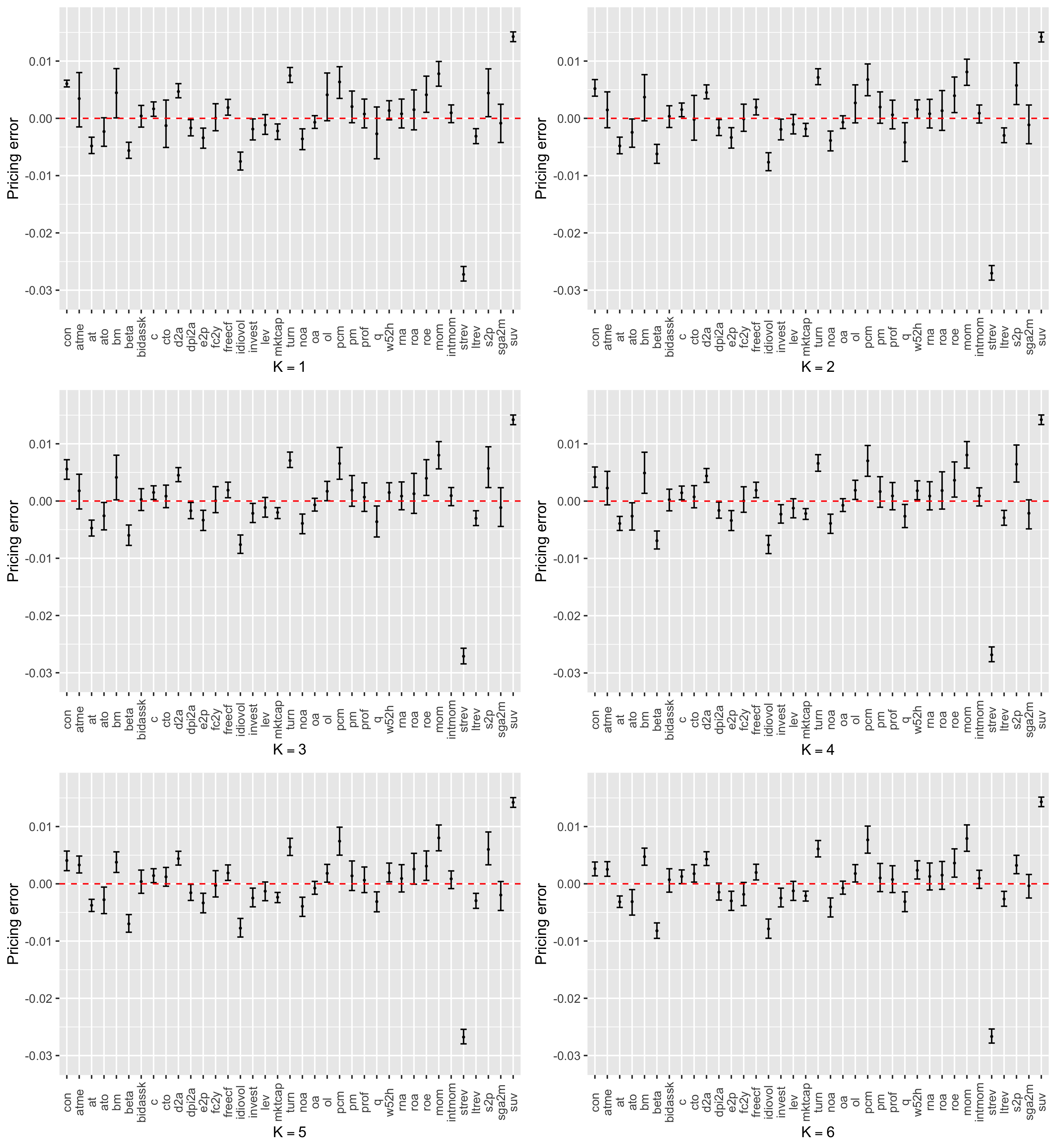
Figure 4: Estimates and $95\%$ confidence intervals of coefficients in $alpha$ under linear specifications of $\alpha(\cdot)$ and $\beta(\cdot)$

We also examine the estimated contribution of each individual characteristic to the conditional pricing error as we vary the number of factors. In Figure 4, we report the estimates and their associated $95\%$ confidence intervals for the coefficients in the linear specification. We find that increasing the number of factors does not affect the estimates and confidence intervals significantly. This implies that the estimation of $alpha$ is not sensitive to the number of factors, in stark contrast to the estimates of Kellyetal_Characteristics_2019.

We further estimate the model with ten factors over different subsample periods by dividing the entire sample (starting in January 1970 and ending in May 2014) into five-year intervals. Since our method does not requite a large $T$, we are able to reliably estimate the factor model over such short subsamples. We report the key results from this subsample analysis in Figure 5. As shown in the panels on the left side of the figure, the mispricing errors under nonlinear models are significantly smaller than under the linear model, which is consistent with the findings of strong nonlinearity for model specification. In the linear case, the average squared pricing errors are the highest in the beginning of the sample, in 1970-1974, dropping subsequently, rising over the equity market “boom” period of the 1990s and peaking in the early 2000s, then falling sharply. In the nonlinear cases, the pattern looks a bit different, but in both of the nonlinear specifications the pricing errors spike around 1990-1994, falling afterwards to roughly the same level towards the end of the sample as in the linear case.

The share of both time-series and cross-sectional variation in returns that is attributable to the common factors, as evidenced by the $R^{2}$ measures reported in the right-side panels of Figure 5, is similar across the different model specifications. More importantly, in Figure 5, we document that all the reported $R^{2}$ measures decline starting in 1970, reach their trough in the mid-1990s, and then continue to rise until the end of our sample in 2014. This observation is consistent with the findings in Campbell2001have and Campbell2022idiosyncratic: Campbell2001have document that there has been a noticeable increase in firm-level volatility from 1962 to 1997; extending this analysis until the year 2021, Campbell2022idiosyncratic find that the idiosyncratic volatility declined after spiking in 1999-2000.

We plot the estimated coefficients with which the characteristics enter the alpha function in different subsample periods with ten factors for six important characteristics under the linear model with 36 characteristics in Figure 6. From the figure, we can conclude that the coefficients for “market capitalization”, “book-to-market ratio” and “momentum” are significantly different from zero in almost all of the subsample periods. The signs of associated coefficients are consistent with the traditional views in FamaFrench_Commonrisk_1993 and FamaFrench_FiveFactor_2015. In parallel with the results in Figure 5, the magnitude of respective coefficients is significantly larger during 1995-2004 compared to other subsample periods, indicating that there is more substantial mispricing associated with these characteristics during that time period. At the same time, the “investment” and “profitability” characteristics are not statistically significantly associated with alpha across different sample periods, suggesting that they capture exposure to common sources of risk.

In order to examine the performance of arbitrage portfolios constructed using different subsample periods, in Figure 7, we plot the out-of-sample average annualized excess returns and associated Sharpe ratios of arbitrage portfolios using expanding window estimation starting from the second year in each subsample period. Consistent with the findings in Figure 5, we observe the significant decline of mispricing errors since 2000. From the right panel of Figure 7, we conclude that the decline of arbitrage portfolio Sharpe ratios is due to the decrease of portfolio’s average returns rather than increase in standard deviations.

Finally, we assess the out-of-sample fit of the conditional factor model with ten factors in different sample periods; and report the associated results in Figure 8. Overall, the estimated factors are able to explain substantial proportion of cross-sectional variation of individual stock returns out-of-sample, as well as the common time-series variation in returns, but measures of fit vary over time. Similar to Figure 5 discussed above, the findings are consistent with the observation that firm-level volatility increases from 1970 until about 1999 and then decreases, as in Campbell2001have and Campbell2022idiosyncratic. Similarly, the ability of the factor models to explain the cross-section of average stock returns deteriorates between 1980 and mid-1990s, and improves thereafter.

7 Conclusion

In this paper we developed a simple and tractable sieve estimation of conditional factor models with time-varying covariances and latent factors, as well as a weighted-bootstrap procedure for conducting inference on the intercept and factor loading functions. We established large sample properties of the estimators and validity of the tests for large $N$, even when $T$ is small. These results enable us to estimate conditional (dynamic) behavior of a large set of individual assets from a number of characteristics exhibiting nonlinearity without the need to pre-specify factors, while allowing us to disentangle the $alpha$ from betas. We applied these methods to explain the cross-sectional differences of individual stock returns in the US market. We found strong evidence of conditional factor structure as well as nonlinearity in conditional $alpha$ and beta functions. Importantly, although only one or two factors are selected by the formal tests, even when a large number of common factors is considered, conditional pricing errors remain large, resulting in arbitrage portfolios with high Sharpe ratios (typically above 3). We also document the significant decline of pricing errors since 2000.

Table I: Results under linear specifications of $\alpha(\cdot)$ and $\beta(\cdot)$ with 36 characteristics^†

Unrestricted ($\alpha(\cdot)\neq 0$)
$K$	$R^{2}_{K}$	$R^{2}$	$R^{2}_{T,N}$	$R^{2}_{N,T}$	$R^{2}_{f}$	$R^{2}_{f,T,N}$	$R^{2}_{f,N,T}$	$R^{2}_{f,O}$	$R^{2}_{f,T,N,O}$	$R^{2}_{f,N,T,O}$	Mean	Std	$SR_{\alpha}$	$SR_{f,K}$	$SR_{f}$
$1^{\ast}$	26.55	2.54	1.37	0.36	2.07	0.59	0.11	6.23	3.79	5.65	1.72	0.54	3.18	0.61	0.61
2	36.42	4.52	2.43	1.76	4.08	1.75	1.37	13.59	10.63	11.28	1.74	0.52	3.36	-0.12	0.55
3	45.03	5.70	3.70	2.70	5.24	2.95	2.31	14.09	11.10	11.67	1.77	0.50	3.56	-0.34	0.46
4	52.55	11.69	8.55	9.27	11.28	7.92	8.69	14.74	12.15	12.11	1.77	0.47	3.74	0.02	0.44
5	58.65	11.90	8.73	9.48	11.49	7.99	8.90	15.17	12.90	12.42	1.70	0.44	3.84	0.42	0.53
6	64.20	13.90	10.30	11.80	13.53	9.79	11.24	15.38	13.19	12.63	1.68	0.44	3.78	0.23	0.57
7	69.15	15.59	12.23	13.76	15.23	11.71	13.23	15.62	13.32	12.87	1.63	0.44	3.73	0.60	0.68
8	72.84	15.93	12.59	13.98	15.56	12.00	13.44	15.90	13.58	13.12	1.61	0.42	3.79	0.24	0.72
9	76.26	16.08	12.67	14.19	15.72	12.15	13.64	16.13	13.83	13.33	1.61	0.42	3.80	-0.06	0.69
10	79.15	16.23	12.82	14.35	15.87	12.34	13.80	16.29	14.06	13.47	1.60	0.42	3.82	0.11	0.67
$K$	$R^{2}_{O}$	$R^{2}_{T,N,O}$	$R^{2}_{N,T,O}$	$p_{\alpha}$	$p_{\text{lin}}$
1-10	0.54	0.64	0.21	$<1\%$	$<1\%$

• $K$: the number of factor specified (^∗ denotes the estimated one by our methods); Fama-MacBeth cross sectional regression $R^{2}$: $R^{2}_{\tilde{Y}}=20.72\%$; $R^{2}_{K}$ measures the variations of managed portfolios captured by different numbers of factors from PCA; $R^{2}$, $R^{2}_{T,N}$, $R^{2}_{N,T}$: various in-sample $R^{2}$’s ($\%$), see (24)-(26); $R^{2}_{f}$, $R^{2}_{f,T,N}$, $R^{2}_{f,N,T}$: various in-sample $R^{2}$’s ($\%$) without $\alpha(\cdot)$, see (27)-(29); $R^{2}_{O}$, $R^{2}_{T,N,O}$, $R^{2}_{N,T,O}$: various out-sample predictive $R^{2}$’s ($\%$), see (30)-(32); $R^{2}_{f,O}$, $R^{2}_{f,T,N,O}$, $R^{2}_{f,N,T,O}$: various out-sample fits $R^{2}$’s ($\%$), see (34)-(36); Mean: out-of-sample annualized means of the pure-alpha arbitrage strategy($\%$); Std: out-of-sample annualized standard deviations of the pure-alpha arbitrage strategy($\%$); $SR_{\alpha}$: out-of-sample annualized Sharpe ratios of the pure-alpha arbitrage strategy; $SR_{f,K}$: out-of-sample annualized Sharpe ratios of the realized $K$-th out-of-sample factor; $SR_{f}$: out-of-sample annualized Sharpe ratios of the MVE portfolio of $K$ out-of-sample factors; $p_{\alpha}$ and $p_{\text{lin}}$ are the p-values of alpha test ($\alpha(\cdot)=0$) and model specification test (joint linearity of $\alpha(\cdot)$ and $\beta(\cdot)$), separately.

Table II: Results under piecewise linear specifications of $\alpha(\cdot)$ and $\beta(\cdot)$ with 18 characteristics and one internal knot^†

Unrestricted ($\alpha(\cdot)\neq 0$)
$K$	$R^{2}_{K}$	$R^{2}$	$R^{2}_{T,N}$	$R^{2}_{N,T}$	$R^{2}_{f}$	$R^{2}_{f,T,N}$	$R^{2}_{f,N,T}$	$R^{2}_{f,O}$	$R^{2}_{f,T,N,O}$	$R^{2}_{f,N,T,O}$	Mean	Std	$SR_{\alpha}$	$SR_{f,K}$	$SR_{f}$
1	41.61	5.94	3.47	3.60	5.52	2.99	3.11	11.27	7.81	8.93	2.46	0.69	3.54	0.51	0.51
$2^{\ast}$	59.05	9.56	6.17	6.91	9.18	5.67	6.33	14.04	11.31	11.29	2.39	0.57	4.22	0.18	0.53
3	64.47	10.42	6.78	7.96	10.03	6.27	7.38	14.64	11.93	11.95	2.36	0.57	4.17	0.45	0.64
4	68.99	13.83	10.26	11.52	13.40	9.80	10.90	15.44	12.98	12.54	2.19	0.53	4.12	0.85	1.04
5	72.33	14.32	10.73	11.98	13.91	10.29	11.38	15.78	13.43	12.89	2.19	0.51	4.26	-0.03	0.93
6	75.35	14.71	10.97	12.40	14.29	10.55	11.86	16.20	14.16	13.18	1.95	0.49	3.96	1.23	1.62
7	77.63	15.28	11.78	12.99	14.84	11.27	12.42	16.45	14.34	13.37	1.90	0.48	3.93	0.45	1.66
8	80.83	15.44	11.98	13.16	15.10	11.59	12.73	16.59	14.50	13.52	1.73	0.47	3.66	1.11	1.99
9	82.88	15.84	12.33	13.49	15.48	11.87	13.05	16.86	14.69	13.81	1.31	0.40	3.26	1.81	2.80
10	85.61	16.39	12.89	13.93	15.71	11.80	13.14	16.98	14.72	13.86	0.88	0.28	3.14	1.72	3.33
$K$	$R^{2}_{O}$	$R^{2}_{T,N,O}$	$R^{2}_{N,T,O}$	$p_{\alpha}$	$p_{\text{lin}}$
1-10	0.59	0.64	0.28	$<1\%$	$<1\%$

• $K$: the number of factor specified (^∗ denotes the estimated one by our methods); Fama-MacBeth cross sectional regression $R^{2}$: $R^{2}_{\tilde{Y}}=20.72\%$; $R^{2}_{K}$ measures the variations of managed portfolios captured by different numbers of factors from PCA; $R^{2}$, $R^{2}_{T,N}$, $R^{2}_{N,T}$: various in-sample $R^{2}$’s ($\%$), see (24)-(26); $R^{2}_{f}$, $R^{2}_{f,T,N}$, $R^{2}_{f,N,T}$: various in-sample $R^{2}$’s ($\%$) without $\alpha(\cdot)$, see (27)-(29); $R^{2}_{O}$, $R^{2}_{T,N,O}$, $R^{2}_{N,T,O}$: various out-sample predictive $R^{2}$’s ($\%$), see (30)-(32); $R^{2}_{f,O}$, $R^{2}_{f,T,N,O}$, $R^{2}_{f,N,T,O}$: various out-sample fits $R^{2}$’s ($\%$), see (34)-(36); Mean: out-of-sample annualized means of the pure-alpha arbitrage strategy($\%$); Std: out-of-sample annualized standard deviations of the pure-alpha arbitrage strategy($\%$); $SR_{\alpha}$: out-of-sample annualized Sharpe ratios of the pure-alpha arbitrage strategy; $SR_{f,K}$: out-of-sample annualized Sharpe ratios of the realized $K$-th out-of-sample factor; $SR_{f}$: out-of-sample annualized Sharpe ratios of the MVE portfolio of $K$ out-of-sample factors; $p_{\alpha}$ and $p_{\text{lin}}$ are the p-values of alpha test ($\alpha(\cdot)=0$) and model specification test (joint linearity of $\alpha(\cdot)$ and $\beta(\cdot)$), separately.

Table III: Results under piecewise linear specifications of $\alpha(\cdot)$ and $\beta(\cdot)$ with 12 characteristics and two internal knots^†

Unrestricted ($\alpha(\cdot)\neq 0$)
$K$	$R^{2}_{K}$	$R^{2}$	$R^{2}_{T,N}$	$R^{2}_{N,T}$	$R^{2}_{f}$	$R^{2}_{f,T,N}$	$R^{2}_{f,N,T}$	$R^{2}_{f,O}$	$R^{2}_{f,T,N,O}$	$R^{2}_{f,N,T,O}$	Mean	Std	$SR_{\alpha}$	$SR_{f,K}$	$SR_{f}$
1	42.78	5.57	2.98	3.32	5.19	2.54	2.83	11.08	7.57	8.77	3.29	0.99	3.33	0.54	0.54
$2^{\ast}$	61.36	9.56	5.97	6.87	9.18	5.51	6.26	13.85	11.12	10.99	3.01	0.80	3.78	0.47	0.70
3	67.77	10.59	6.65	7.88	10.20	6.15	7.29	14.66	12.25	11.83	2.94	0.80	3.69	0.51	0.78
4	72.86	13.62	10.09	11.35	13.17	9.64	10.67	15.39	13.53	12.53	2.97	0.78	3.81	-0.18	0.59
5	76.92	14.14	10.43	12.01	13.73	10.01	11.48	15.82	13.94	12.90	2.98	0.76	3.91	-0.04	0.56
6	80.63	14.94	11.45	12.75	14.42	10.51	12.05	16.16	14.20	13.22	1.51	0.41	3.73	2.47	2.55
7	84.29	15.17	11.59	12.94	14.76	10.77	12.447	16.57	14.59	13.57	1.01	0.33	3.09	1.87	3.20
8	87.42	15.45	11.87	13.23	15.26	11.47	12.98	16.94	14.83	13.88	0.73	0.22	3.36	1.25	3.29
9	89.11	16.33	12.68	13.94	16.16	12.31	13.72	17.12	15.00	14.09	0.71	0.20	3.62	0.28	3.24
10	90.72	16.54	12.91	14.17	16.38	12.54	13.95	17.30	15.19	14.29	0.69	0.18	3.90	0.23	3.19
$K$	$R^{2}_{O}$	$R^{2}_{T,N,O}$	$R^{2}_{N,T,O}$	$p_{\alpha}$	$p_{\text{lin}}$
1-10	0.57	0.57	0.27	$<1\%$	$<1\%$

• $K$: the number of factor specified (^∗ denotes the estimated one by our methods); Fama-MacBeth cross sectional regression $R^{2}$: $R^{2}_{\tilde{Y}}=20.72\%$; $R^{2}_{K}$ measures the variations of managed portfolios captured by different numbers of factors from PCA; $R^{2}$, $R^{2}_{T,N}$, $R^{2}_{N,T}$: various in-sample $R^{2}$’s ($\%$), see (24)-(26); $R^{2}_{f}$, $R^{2}_{f,T,N}$, $R^{2}_{f,N,T}$: various in-sample $R^{2}$’s ($\%$) without $\alpha(\cdot)$, see (27)-(29); $R^{2}_{O}$, $R^{2}_{T,N,O}$, $R^{2}_{N,T,O}$: various out-sample predictive $R^{2}$’s ($\%$), see (30)-(32); $R^{2}_{f,O}$, $R^{2}_{f,T,N,O}$, $R^{2}_{f,N,T,O}$: various out-sample fits $R^{2}$’s ($\%$), see (34)-(36); Mean: out-of-sample annualized means of the pure-alpha arbitrage strategy($\%$); Std: out-of-sample annualized standard deviations of the pure-alpha arbitrage strategy($\%$); $SR_{\alpha}$: out-of-sample annualized Sharpe ratios of the pure-alpha arbitrage strategy; $SR_{f,K}$: out-of-sample annualized Sharpe ratios of the realized $K$-th out-of-sample factor; $SR_{f}$: out-of-sample annualized Sharpe ratios of the MVE portfolio of $K$ out-of-sample factors; $p_{\alpha}$ and $p_{\text{lin}}$ are the p-values of alpha test ($\alpha(\cdot)=0$) and model specification test (joint linearity of $\alpha(\cdot)$ and $\beta(\cdot)$), separately.

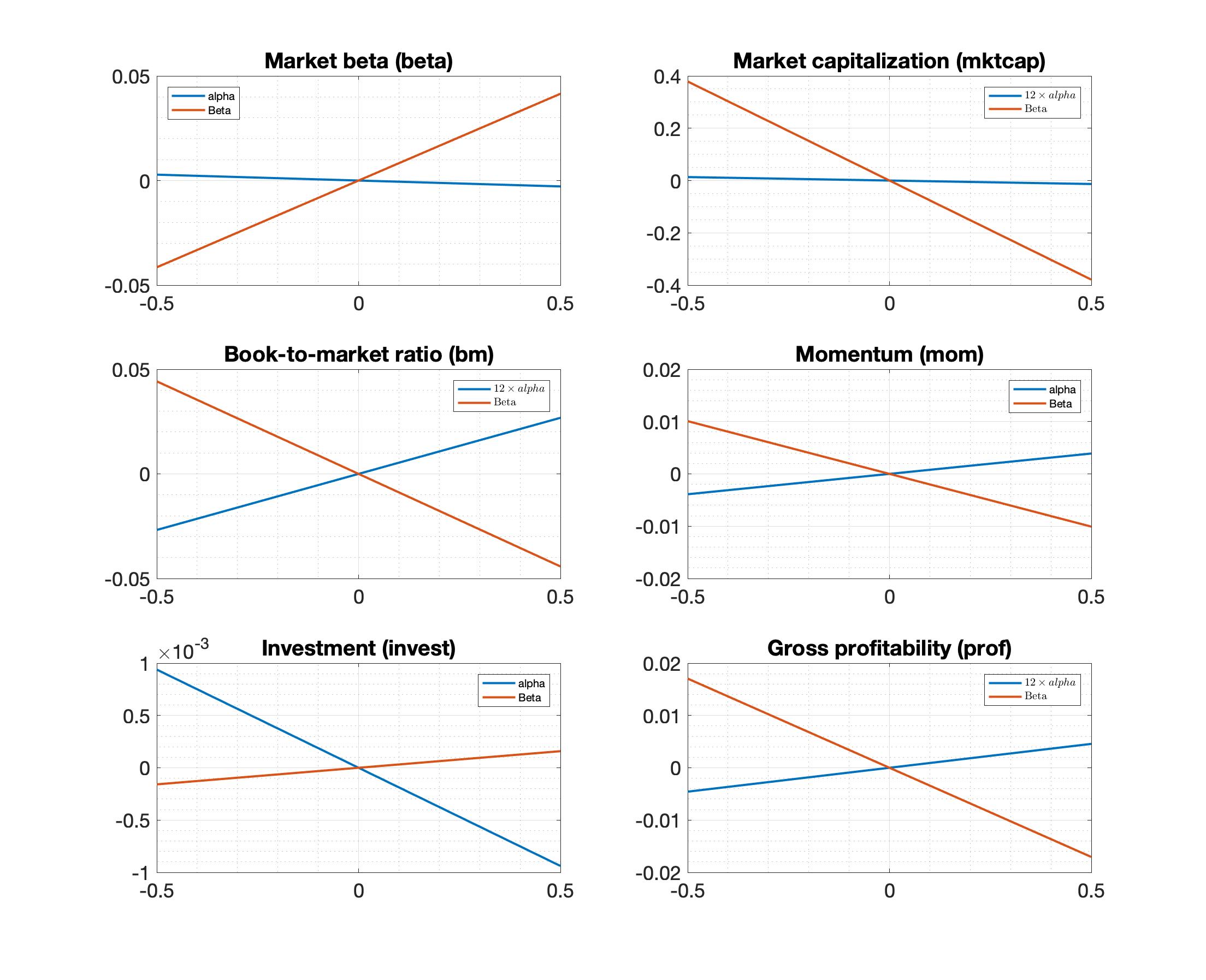
Figure 1: Characteristics-$alpha$ and characteristics-$beta$ plots under linear specifications of $\alpha(\cdot)$ and $\beta(\cdot)$ with 36 characteristics

Notes: the six important characteristics are market capitalization (mktcap), market beta (beta), book-to-market ratio (bm), momentum (mom), investment (invest), and gross profitability (prof). To make the magnitude comparable, the annualized values are reported for some alphas.

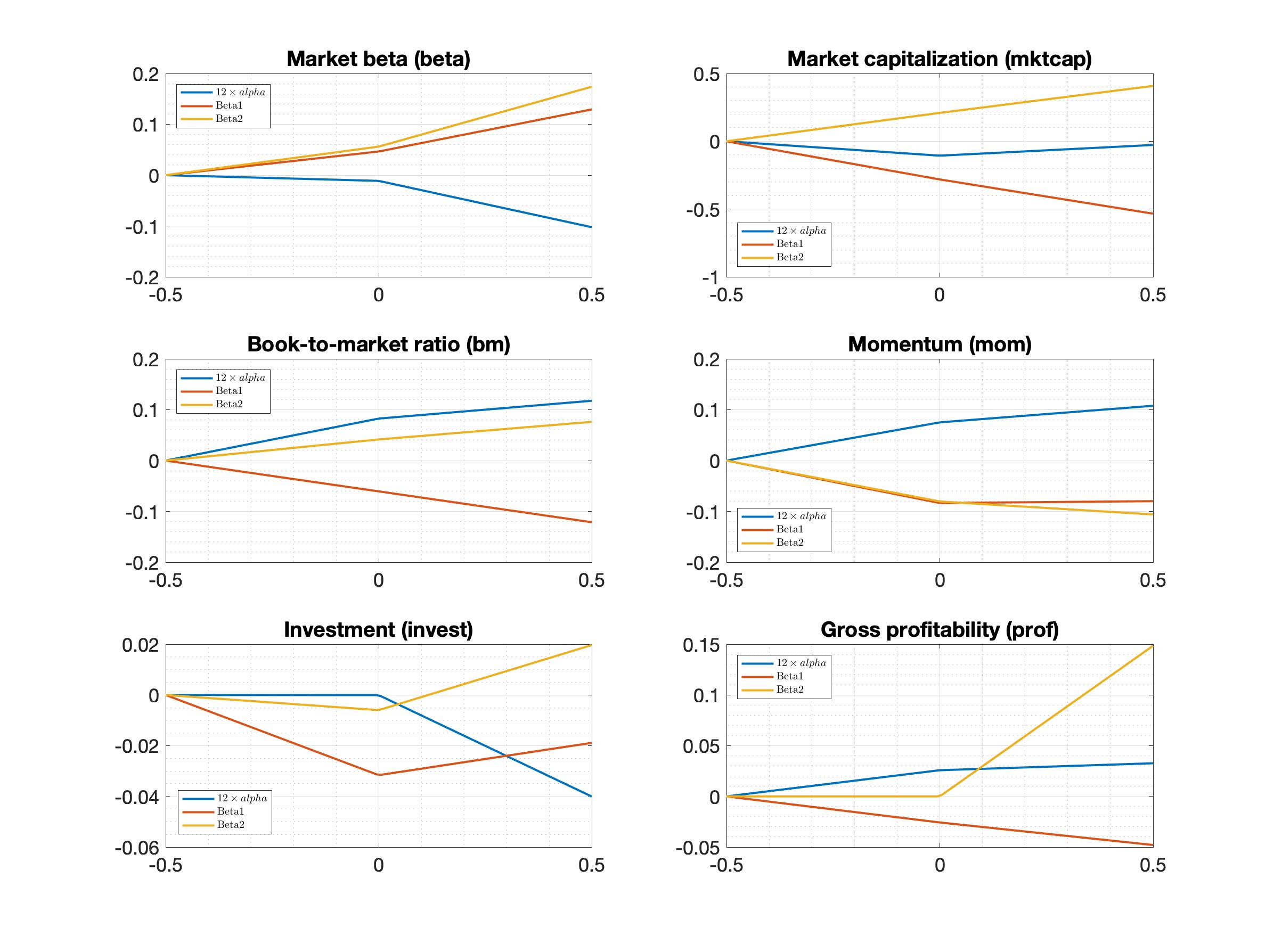
Figure 2: Characteristics-$alpha$ and characteristics-$beta$ plots under continuous piecewise linear specifications of $\alpha(\cdot)$ and $\beta(\cdot)$ with 18 characteristics and one internal knot

Notes: the six important characteristics are market capitalization (mktcap), market beta (beta), book-to-market ratio (bm), momentum (mom), investment (invest), and gross profitability (prof). To make the magnitude comparable, the annualized $alpha$ is reported.

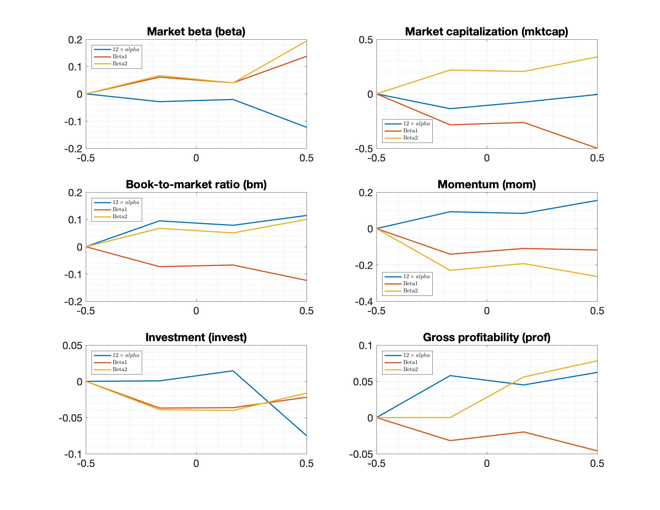
Figure 3: Characteristics-alpha and characteristics-beta plots under continuous piecewise linear specifications of $\alpha(\cdot)$ and $\beta(\cdot)$ with 12 characteristics and two internal knots

Notes: the six important characteristics are market capitalization (mktcap), market beta (beta), book-to-market ratio (bm), momentum (mom), investment (invest), and gross profitability (prof). To make the magnitude comparable, the annualized alpha is reported.

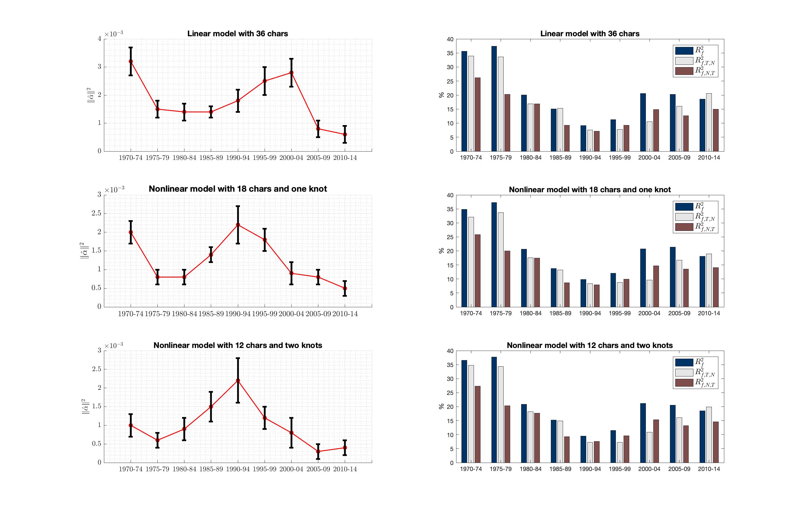
Figure 5: Estimates and $95\%$ confidence intervals of $\|\alpha\|^{2}$ and $R^{2}$s with $K=10$ from common factor part in different subsample periods

Notes: the left panel plots $\|\hat{\alpha}\|^{2}$ and associated 95% confidence interval in different subsample periods with $K=10$; the right panel reports $R^{2}_{f}$, $R^{2}_{f,T,N}$, $R^{2}_{f,N,T}$ defined in (27)-(29) in different sample periods with $K=10$. The three rows are corresponding to estimation under linear mode with 36 chars, nonlinear models with 18 chars and one internal knot and 12 chars with two internal knots, separately.

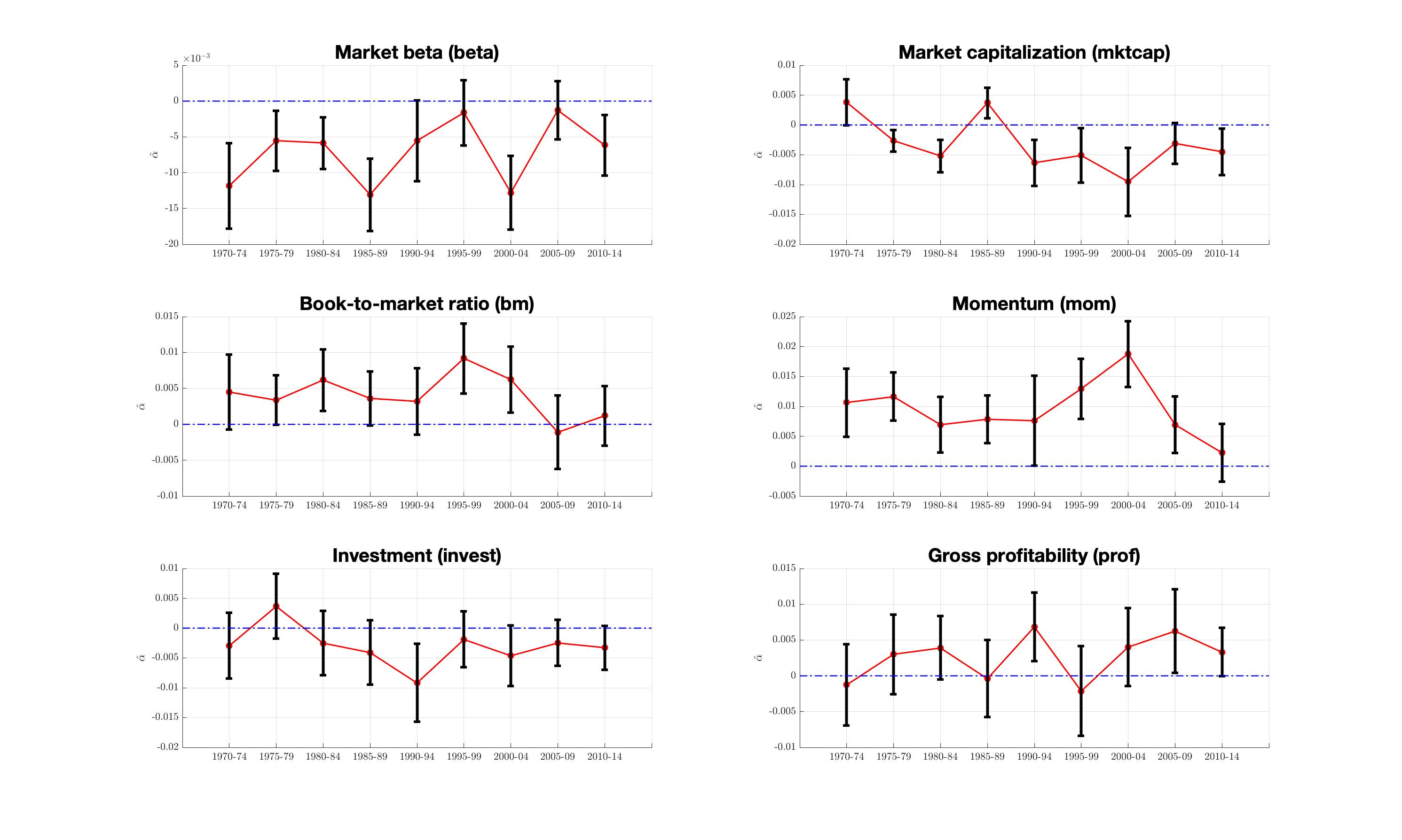
Figure 6: Characteristics-$alpha$ plots under linear specifications of $\alpha(\cdot)$ and $\beta(\cdot)$ with $K=10$ and 36 characteristics in different subsample periods

Notes: the graph plots the elements in $\hat{\alpha}$ with $K=10$ for six important characteristics and associated 95% confidence interval across different subsample periods.

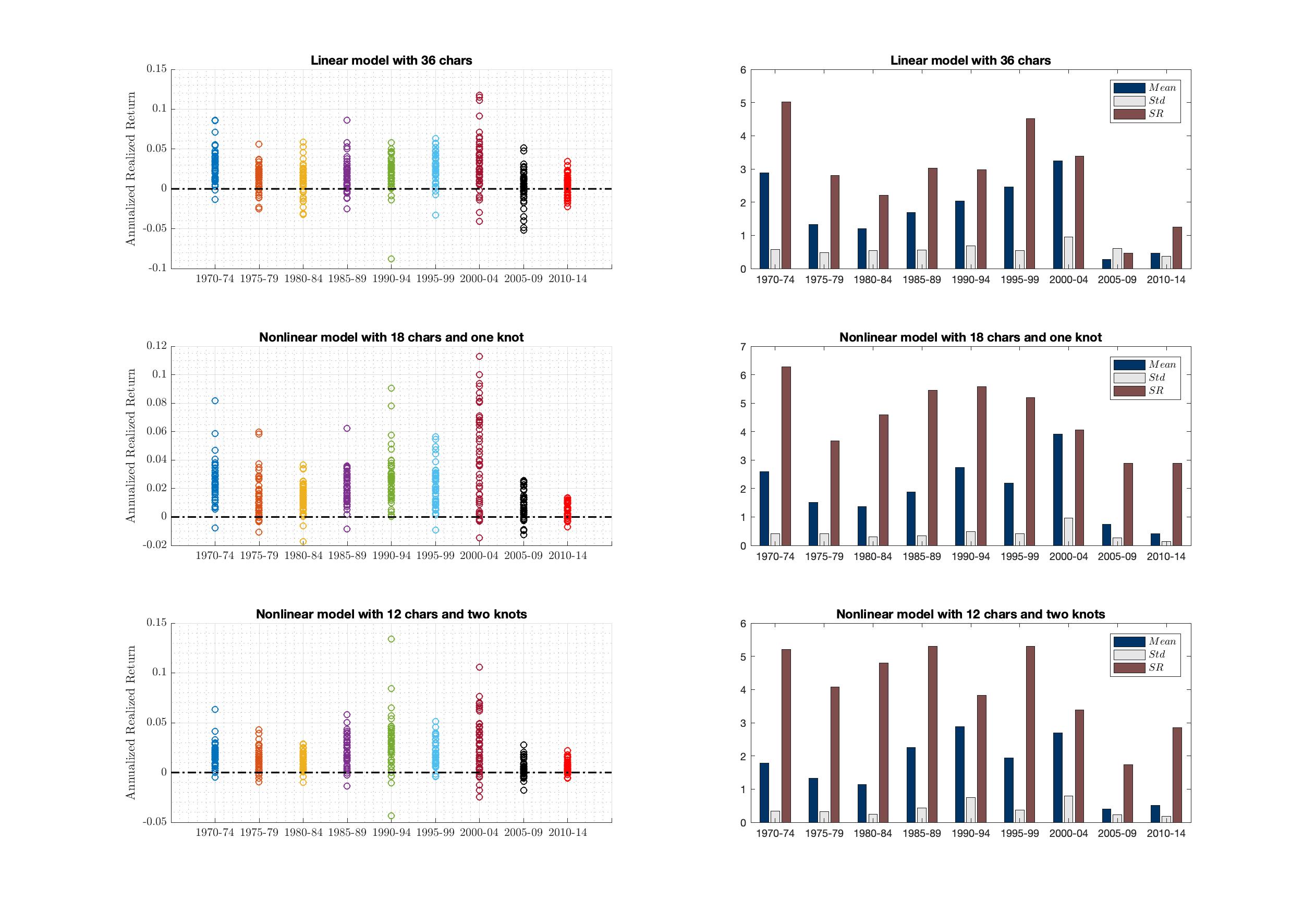
Figure 7: Annualized realized excess returns of arbitrage portfolio and the associated annualized Sharpe ratios with $K=10$ in different subsample periods

Notes: the graph plots the annualized realized excess returns of arbitrage portfolio constructed with expanding estimation; and the associated annualized Sharpe ratios with $K=10$ in different subsample periods. The three rows are corresponding to estimation under linear mode with 36 chars, nonlinear models with 18 chars and one internal knot and 12 chars with two internal knots, separately.

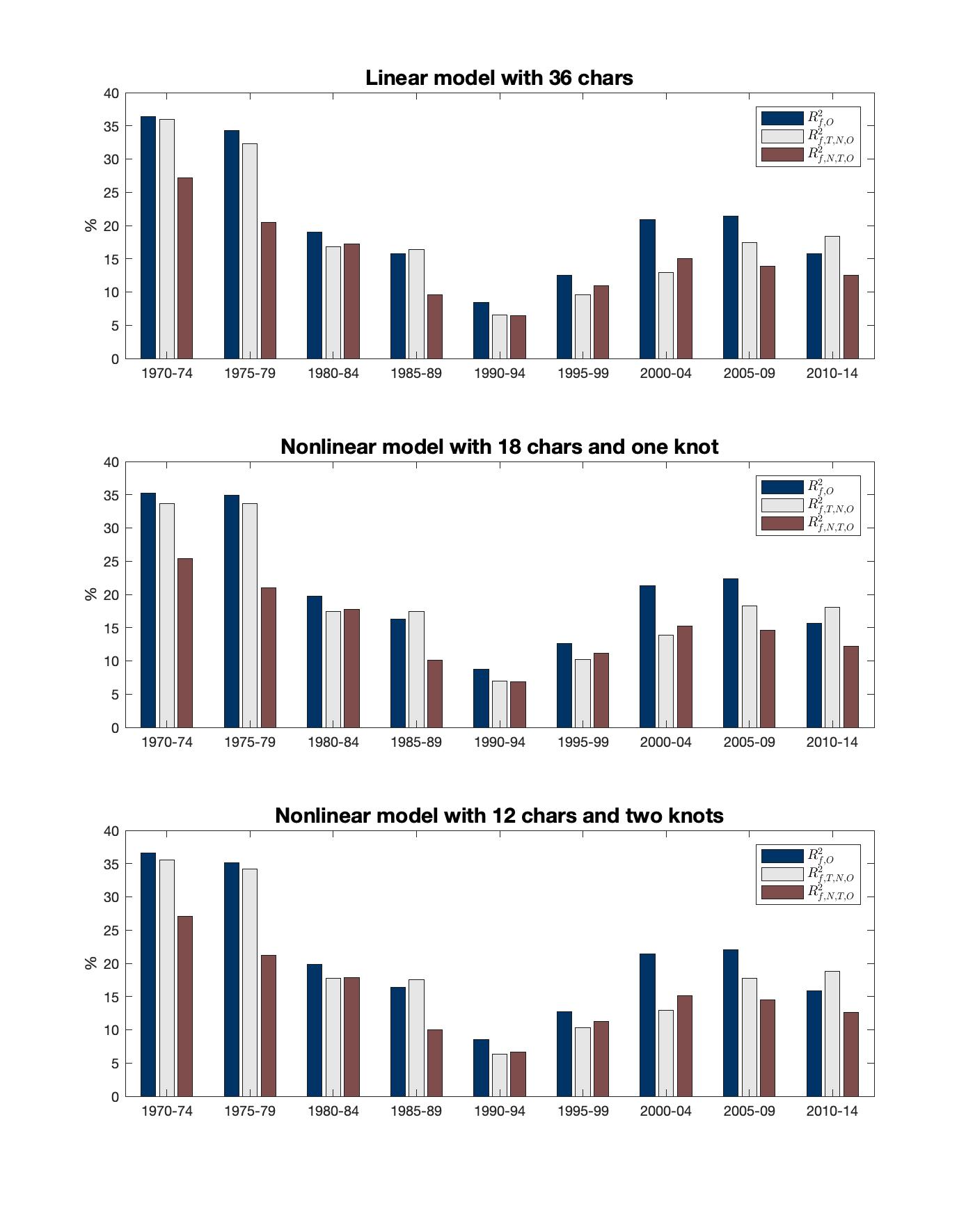
Figure 8: Out-of-sample fits $R^{2}$s with $K=10$ in different subsample periods

Notes: the panel plots out-of-sample fits $R^{2}$s with $K=10$ and without the restriction $\alpha(\cdot)=0$ in different subsample periods. The three rows are corresponding to estimation under linear mode with 36 chars, nonlinear models with 18 chars and one internal knot and 12 chars with two internal knots, separately.

Appendix Appendix A Assumptions

Assumption A.1 (Basis functions).

(i) There are positive constants $c_{\min}$ and $c_{\max}$ such that: with probability approaching one (as $N\to\infty$),

$$c_{\min}<\min_{t\leq T}\lambda_{\min}(\hat{Q}_{t})\leq\max_{t\leq T}\lambda_{\max}(\hat{Q}_{t})<c_{\max},$$

where $\hat{Q}_{t}=\Phi(Z_{t})^{\prime}\Phi(Z_{t})/N$; (ii) $\max_{m\leq M,j\leq J,i\leq N,t\leq T}E[\phi^{2}_{j}(z_{it,m})]<\infty$.

Since $\hat{Q}_{t}=\sum_{i=1}^{N}\phi(z_{it})\phi(z_{it})^{\prime}/N$ is a $JM\times JM$ matrix with $JM$ much smaller than $N$, Assumption A.1(i) can follow from the law of large numbers for finite $T$ and its uniform variant for $T\to\infty$; see Proposition C.1 for a set of sufficient conditions. The conditions can be easily verified for B-spline, Fourier series, and polynomials basis functions. In particular, we allow $Z_{t}$ to be nonstationary over $t$. When $Z_{t}$ is not changing over $t$, Assumption A.1 reduces to Assumptions 3.3 of Fanetal_ProjectedPCA_2016.

Assumption A.2 (Factor loading functions and factors).

There are positive constants $d_{\min}$ and $d_{\max}$ such that: (i) $d_{\min}<\lambda_{\min}(B^{\prime}B)\leq\lambda_{\max}(B^{\prime}B)<d_{\max}$; (ii) $\max_{t\leq T}\|f_{t}\|<d_{\max}$; (iii) $\lambda_{\min}(F^{\prime}M_{T}F/T)>d_{\min}$; (iv) $\max_{k\leq K,m\leq M}\sup_{z}|\delta_{km,J}(z)|$ $=O(J^{-\kappa})$ and $\max_{m\leq M}\sup_{z}|r_{m,J}(z)|=O(J^{-\kappa})$ for some constant $\kappa>1/2$.

Assumption A.2(i) is similar to the pervasive condition on the factor loadings in StockWatson_PCA_2002. Similar assumptions also are imposed in Assumption B of Bai_Inferential_2003 and Assumption 4.1(ii) of Fanetal_ProjectedPCA_2016. For simplicity of presentation, we assume that $f_{t}$’s are nonrandom. Since the dimension of $B$ is $JM\times K$, Assumption A.2(i) requires $JM\geq K$. Since the rank of $M_{T}$ is $T-1$, Assumption A.2(iii) requires $T\geq K+1$, which implies $T\geq 2$. These two requirements are not restrictive, since we assume $K$ is fixed. Assumption A.2(iv) is standard in the sieve literature. It can be easily satisfied by using B-spline or polynomials basis functions under certain smoothness of $\alpha(\cdot)$ and $\beta(\cdot)$; see, for example, Lorentz_Approximation_1986 and Chen_Handbook_2007.

Assumption A.3 (Data generating process).

(i)$\{\varepsilon_{t}\}_{t\leq T}$ is independent of $\{Z_{t}\}_{t\leq T}$; (ii) $E[\varepsilon_{it}]=0$ for all $i\leq N$ and $t\leq T$; (iii) there is $0<C_{1}<\infty$ such that

$$\max_{i\leq N,t\leq T}\sum_{j=1}^{N}|E[\varepsilon_{it}\varepsilon_{jt}]|<C_{1}\text{ and }\frac{1}{NT}\sum_{i=1}^{N}\sum_{j=1}^{N}\sum_{t=1}^{T}\sum_{s=1}^{T}|E[\varepsilon_{it}\varepsilon_{js}]|<C_{1}.$$

Assumption A.3(iii) requires $\{\varepsilon_{it}\}_{i\leq N,t\leq T}$ to be weakly dependent over both $i$ and $t$, and is commonly imposed for high-dimensional factor analysis; see, for example, StockWatson_PCA_2002, Bai_Inferential_2003, and Fanetal_ProjectedPCA_2016. When $Z_{t}$ is not changing over $t$, Assumption A.3 reduces to Assumptions 3.4 (i) and (iii) of Fanetal_ProjectedPCA_2016.

Assumption A.4 (Intercept function).

$a^{\prime}B=0$ and $\|a\|<C_{0}$ for some $0<C_{0}<\infty$.

Assumption A.4 is needed for the identification of $\alpha(\cdot)$. Similar assumption is imposed in Connoretal_EfficientFFFactor_2012 and Assumption 3.1(i) of Kimetal_Arbitrage_2019.

Assumption A.5 (Rate of convergence).

(i) $\max_{m\leq M,j\leq J,i\leq N,t\leq T}E[\phi^{4}_{j}(z_{it,m})]<\infty$; (ii) $0<\min_{i\leq N,t\leq T}\lambda_{\min}(Q_{it})\leq\max_{i\leq N,t\leq T}\lambda_{\max}(Q_{it})<\infty$, where $Q_{it}=E[\phi(z_{it})\phi(z_{it})^{\prime}]$; (iii) $\{z_{it}\}_{i\leq N,t\leq T}$ are independent across $i\leq N$; (iv) there is $0<C_{2}<\infty$ such that

$$\max_{t\leq T}\frac{1}{N^{2}}\sum_{i=1}^{N}\sum_{j=1}^{N}\sum_{k=1}^{N}\sum_{\ell=1}^{N}|E[\varepsilon_{it}\varepsilon_{jt}\varepsilon_{kt}\varepsilon_{\ell t}]|<C_{2}$$

and

$$\frac{1}{N^{2}T}\sum_{t=1}^{T}\left(\sum_{s=1}^{T}\sum_{i=1}^{N}\sum_{j=1}^{N}|E[\varepsilon_{it}\varepsilon_{js}]|\right)^{2}<C_{2}.$$

Assumptions A.1-A.4 allow us to establish a preliminary rate of the estimators in Theorem C.1. Assumption A.5 is an additional assumption that we need to establish a fast rate in Theorem 3.1. Assumption A.5(i) strengthens Assumption A.1(ii). Assumption A.5(ii) requires that the second moment matrix $E[\phi(z_{it})\phi(z_{it})^{\prime}]$ is bounded and nonsingular for all $i$ and $t$, which is widely used in the sieve literature; see, for example, Newey_SeriesEstimator_1997 and Huang_Series_1998. Assumption A.5(iii) is commonly imposed in the sieve literature, which is used to justify the asymptotic convergence of $\hat{Q}_{t}$. Assumption A.5(iv) allows for weak dependence of $\{\varepsilon_{it}\}_{i\leq N,t\leq T}$ over both $i$ and $t$. The second condition is similar to the second condition in Assumption A.3(iii); both are satisfied if $\max_{t\leq T}\sum_{s=1}^{T}\sum_{i=1}^{N}\sum_{j=1}^{N}$ $|E[\varepsilon_{it}\varepsilon_{js}]/N$ is bounded.

Assumption A.6 (Asymptotic distribution).

(i) $(F^{\prime}M_{T}F/T)B^{\prime}B$ has distinct eigenvalues; (ii) $\{\varepsilon_{it}\}_{i\leq N,t\leq T}$ are independent across $i\leq N$; (iii) there is $0<C_{3}<\infty$ such that

$$\max_{i\leq N}\frac{1}{T^{2}}\sum_{t=1}^{T}\sum_{s=1}^{T}\sum_{u=1}^{T}\sum_{v=1}^{T}|E[\varepsilon_{it}\varepsilon_{is}\varepsilon_{iu}\varepsilon_{iv}]|<C_{3}.$$

Assumption A.6 is needed in Theorem 3.2. The distinct eigenvalue condition in Assumption A.6(i) is necessary to establish the asymptotic normality, as known in the literature; see, for example, Bai_Inferential_2003 and ChenFang_ImprovedInference_2017. Assumption A.6(ii) imposes independence of $\{\varepsilon_{it}\}_{i\leq N,t\leq T}$ across $i$ for simplicity. Assumption A.6(iii) allows for weak dependence of $\{\varepsilon_{it}\}_{i\leq N,t\leq T}$ over $t$.

Assumption A.7 (Bootstrap).

(i) $\{w_{i}\}_{i\leq N}$ is a sequence of independently and identically distributed positive random variables with $E[w_{i}]=1$ and $var(w_{i})=\omega_{0}>0$, and is independent of $\{Z_{t},\varepsilon_{t}\}_{t\leq T}$; (ii) there are positive constants $e_{\min}$ and $e_{\max}$ such that: with probability approaching one (as $N\to\infty$),

$$e_{\min}<\min_{t\leq T}\lambda_{\min}(\hat{Q}_{t}^{\ast})\leq\max_{t\leq T}\lambda_{\max}(\hat{Q}_{t}^{\ast})<e_{\max},$$

where $\hat{Q}_{t}^{\ast}=\Phi(Z_{t})^{\ast\prime}\Phi(Z_{t})/N$; (iii) $\lambda_{\min}(\Omega)>0$.

Assumption A.7 is needed in Theorem 4.1. Assumption A.7(i) defines the bootstrap weight $w_{i}$ for each $i$. Since $\hat{Q}_{t}^{\ast}=\sum_{i=1}^{N}\phi(z_{it})\phi(z_{it})^{\prime}w_{i}/N$ is a $JM\times JM$ matrix with $JM$ much smaller than $N$, Assumption A.7(ii) can follow from the law of large numbers for finite $T$ and its uniform variant for $T\to\infty$, similar to Assumption A.1(i). Assumption A.7(iii) requires nonsingularity of the variance-covariance matrix $\Omega$.

Assumption A.8 (Specification test).

(i) There are positive constants $g_{\min}$ and $g_{\max}$ such that: with probability approaching one (as $N\to\infty$),

$$g_{\min}<\min_{t\leq T}\lambda_{\min}(Z_{t}^{\prime}Z_{t}/N)\leq\max_{t\leq T}\lambda_{\max}(Z_{t}^{\prime}Z_{t}/N)<g_{\max},$$

(ii) $\max_{i\leq N,t\leq T}E[\|z_{it}\|^{4}]<\infty$; (iii) $\min_{i\leq N,t\leq T}\lambda_{\min}(E[z_{it}z_{it}^{\prime}])>0$; (iv) with probability approaching one (as $N\to\infty$),

$$g_{\min}<\min_{t\leq T}\lambda_{\min}(Z_{t}^{\ast\prime}Z_{t}/N)\leq\max_{t\leq T}\lambda_{\max}(Z_{t}^{\ast\prime}Z_{t}/N)<g_{\max};$$

(v) $\sup_{z}|\alpha(z)|<\infty$ and $\sup_{z}\|\beta(z)\|<\infty$.

Assumption A.8 is needed in Theorem 4.2. Assumptions A.8(i)-(iv) are analogous to Assumptions A.1(i), A.5(i), (ii) and A.7(ii), respectively. When $z_{it}$ is included as a part of $\phi(z_{it})$, which is true in the case of polynomial basis functions, the former are implied by the latter ones. In this case, Assumptions A.8(i)-(iv) thus are redundant.

Assumption A.9 (Determination of $K$).

(i) $0<\min_{t\leq T}\lambda_{\min}(E[\varepsilon_{t}\varepsilon_{t}^{\prime}])\leq\max_{t\leq T}$ $\lambda_{\max}(E[\varepsilon_{t}\varepsilon_{t}^{\prime}])<\infty$; ii) there is $0<C_{4}<\infty$ such that

$$\frac{1}{N^{2}T+T^{2}N}\sum_{t=1}^{T}\sum_{s=1}^{T}\sum_{i=1}^{N}\sum_{j=1}^{N}\sum_{k=1}^{N}\sum_{\ell=1}^{N}|cov(\varepsilon_{it}\varepsilon_{jt},\varepsilon_{ks}\varepsilon_{\ell s})|<C_{4}.$$

Assumption A.9 is needed in Theorem 5.1(i). Assumption A.9(i) requires that the covariance matrix $E[\varepsilon_{t}\varepsilon_{t}^{\prime}]$ is bounded and nonsingular for all $t$. In particular, $\max_{t\leq T}\lambda_{\max}(E[\varepsilon_{t}\varepsilon_{t}^{\prime}])<\infty$ allows for weak dependence of $\{\varepsilon_{it}\}_{i\leq N,t\leq T}$ across $i$. When $\{\varepsilon_{it}\}_{i\leq N,t\leq T}$ are independent across $i$, the condition is satisfied when $\min_{i\leq N,t\leq T}E[\varepsilon_{it}^{2}]>0$ and $\max_{i\leq N,t\leq T}E[\varepsilon_{it}^{2}]<\infty$. Assumption A.9(ii) allows for weak dependence of $\{\varepsilon_{it}\}_{i\leq N,t\leq T}$ over both $i$ and $t$; see Proposition C.2 for a set of sufficient conditions.

Appendix Appendix B Proofs of Main Results

Proof of Theorem 3.1: Let us begin by defining some notation. For $A_{t}=\Delta_{t}\equiv R(Z_{t})+\Delta(Z_{t})f_{t}$ and $\varepsilon_{t}$, let $\tilde{A}_{t}\equiv(\Phi(Z_{t})^{\prime}\Phi(Z_{t}))^{-1}\Phi(Z_{t})^{\prime}A_{t}$ . Let $\tilde{\Delta}\equiv(\tilde{\Delta}_{1},\ldots,\tilde{\Delta}_{T})$ and $\tilde{E}\equiv(\tilde{\varepsilon}_{1},\ldots,\tilde{\varepsilon}_{T})$. Then (9) can be written as

$$\tilde{Y}=a1_{T}^{\prime}+BF^{\prime}+\tilde{\Delta}+\tilde{E},$$ (38)

where $1_{T}$ denote a $T\times 1$ vector of ones. Recall $M_{T}=I_{T}-1_{T}1_{T}^{\prime}/T$. Post-multiplying (38) by $M_{T}$ to remove $a$, we thus obtain

$$\tilde{Y}M_{T}=B(M_{T}F)^{\prime}+\tilde{\Delta}M_{T}+\tilde{E}M_{T}.$$ (39)

Let $V$ be a $K\times K$ diagonal matrix of the first $K$ largest eigenvalues of $\tilde{Y}M_{T}\tilde{Y}^{\prime}/T$. By the definitions of $\hat{B}$ and $\hat{F}$, $(\tilde{Y}M_{T}\tilde{Y}^{\prime}/T)\hat{B}=\hat{B}V$ and $M_{T}\hat{F}=M_{T}\tilde{Y}^{\prime}\hat{B}$. Thus, $\hat{F}^{\prime}M_{T}\hat{F}/T=\hat{B}^{\prime}(\tilde{Y}M_{T}\tilde{Y}^{\prime}/T)\hat{B}=V$ and $H=(F^{\prime}M_{T}\hat{F})(\hat{F}^{\prime}M_{T}\hat{F})^{-1}=(F^{\prime}M_{T}\tilde{Y}^{\prime}\hat{B}/T)V^{-1}$. We may substitute (39) to $(\tilde{Y}M_{T}\tilde{Y}^{\prime}/T)\hat{B}=\hat{B}V$ to obtain

$$\hat{B}-BH=[(\tilde{\Delta}+\tilde{E})M_{T}\tilde{Y}^{\prime}/T]\hat{B}V^{-1}=\sum_{j=1}^{6}D_{j}\hat{B}V^{-1},$$ (40)

where $D_{1}=\tilde{\Delta}M_{T}FB^{\prime}/T$, $D_{2}=\tilde{\Delta}M_{T}\tilde{\Delta}^{\prime}/T$, $D_{3}=D_{6}^{\prime}=\tilde{\Delta}M_{T}\tilde{E}^{\prime}/T$, $D_{4}=\tilde{E}M_{T}FB^{\prime}/T$ and $D_{5}=\tilde{E}M_{T}\tilde{E}^{\prime}/T$. By the definition of $\hat{a}$,

$$\hat{a}-a =-\hat{B}(\hat{B}-BH)^{\prime}a+(I_{JM}-\hat{B}\hat{B}^{\prime})(BH-\hat{B})H^{-1}\bar{f}$$

$$\hskip 14.22636pt+(I_{JM}-\hat{B}\hat{B}^{\prime})\tilde{\Delta}1_{T}/T+(I_{JM}-\hat{B}\hat{B}^{\prime})\tilde{E}1_{T}/T.$$ (41)

where $H^{-1}$ is well defined with probability approaching one by (C.1) and Lemma F.2(ii), and we have used $a^{\prime}B=0$ and $(I_{JM}-\hat{B}\hat{B}^{\prime})\hat{B}=0$. Noting $\hat{B}^{\prime}\hat{B}=I_{K}$, we may substitute (38) to $\hat{F}=\tilde{Y}^{\prime}\hat{B}$ to obtain

$$\hat{F}-F(H^{\prime})^{-1}=1_{T}a^{\prime}(\hat{B}-BH)+F(H^{\prime})^{-1}(BH-\hat{B})^{\prime}\hat{B}+\tilde{\Delta}^{\prime}\hat{B}+\tilde{E}^{\prime}\hat{B}.$$ (42)

where $(H^{\prime})^{-1}$ is well defined with probability approaching one by (C.1) and Lemma F.2(ii), and we have used $a^{\prime}B=0$. Theorem C.1 provides a preliminary rate of $\|\hat{a}-a\|^{2}$, $\|\hat{B}-BH\|^{2}_{F}$ and $\|\hat{F}-F(H^{\prime})^{-1}\|^{2}_{F}$ by using rough bounds based on (40)-(42). To improve the rate of $\|\hat{B}-BH\|^{2}_{F}$, we need to treat $D_{5}\hat{B}$ in as (40) a whole to establish its rate. By the Cauchy-Schwartz inequality and the fact that $\|C+D\|_{F}\leq\|C\|_{F}+\|D\|_{F}$ and $\|CD\|_{F}\leq\|C\|_{2}\|D\|_{F}$, (40) implies

$$\|\hat{B}-BH\|^{2}_{F} \leq 10\|\hat{B}\|^{2}_{2}\|V^{-1}\|^{2}_{2}\left(\sum_{j\neq 5}^{6}\|D_{j}\|^{2}_{F}\right)+2\|V^{-1}\|^{2}_{2}\|D_{5}\hat{B}\|^{2}_{F},$$

$$=O_{p}\left(\frac{1}{J^{2\kappa}}+\frac{J}{N^{2}}+\frac{{J}}{{NT}}\right),$$ (43)

where the equality follows by $J=o(\sqrt{N})$, Lemmas F.1(i)-(iv), F.2(i) and F.6(ii) and the fact that $\|D_{6}\|_{F}=\|D_{3}\|_{F}$. Given the rate of $\|\hat{B}-BH\|^{2}_{F}$ in (Appendix B), the rate of $|\hat{a}-a|^{2}$ immediately follows from the same argument in (C.1). To improve the rate of $\|\hat{F}-F(H^{\prime})^{-1}\|^{2}_{F}$, we need to plug in the expansion of $\hat{B}-BH$ to (Appendix B), and treat $a^{\prime}D_{4}$, $D_{4}^{\prime}\hat{B}$, $D_{5}\hat{B}$ and $\tilde{E}^{\prime}\hat{B}$ as a whole to establish their rates. By the fact that $\|C+D\|_{F}\leq\|C\|_{F}+\|D\|_{F}$ and $\|CD\|_{F}\leq\|C\|_{2}\|D\|_{F}$, combining (40) and (42) implies

$$\|\hat{F}-F(H^{\prime})^{-1}\|_{F} =\left(\sum_{j\neq 4,5}^{6}\|D_{j}\|_{F}\|\hat{B}\|_{2}\|a\|+\|a^{\prime}D_{4}\|\|\hat{B}\|_{2}+\|a\|\|D_{5}\hat{B}\|_{F}\right)\times$$

$$\hskip 22.76228pt\|V^{-1}\|_{2}\|1_{T}\|+\left(\sum_{j\neq 4,5}^{6}\|D_{j}\|_{F}\|\hat{B}\|_{2}+\|D_{4}^{\prime}\hat{B}\|_{F}+\|D_{5}\hat{B}\|_{F}\right)$$

$$\hskip 22.76228pt\times\|F\|_{2}\|H^{-1}\|_{2}\|V^{-1}\|_{2}\|\hat{B}\|_{2}+\|\tilde{\Delta}\|_{F}\|\hat{B}\|_{2}+\|\tilde{E}^{\prime}\hat{B}\|_{F}$$

$$=O_{p}\left(\frac{\sqrt{T}}{J^{\kappa}}+\sqrt{\frac{T}{N}}\right),$$ (44)

where the equality follows by $J=o(\sqrt{N})$, Assumptions A.2(ii) and A.4, Lemmas F.1(i)-(iii), F.2, F.3(i), F.6 and F.7(i) and the fact that $\|D_{6}\|_{F}=\|D_{3}\|_{F}$. Thus, the third result of the theorem follows from (Appendix B). The proofs of the last two results of the theorem are similar to the proofs of the last two results of Theorem C.1.∎

Proof of Theorem 3.2: Let us first look at (Appendix B). The asymptotic distribution can be obtained by choosing large $J$ and assuming $T$ not too large such that the terms with $O_{p}(J^{-2\kappa})$ and $O_{p}(J/N^{2})$ are negligible relative to the term with $O_{p}(J/NT)$. Thus, the asymptotic distribution is determined by the term with $O_{p}(J/NT)$. Specifically, by the fact that $\|C+D\|_{F}\leq\|C\|_{F}+\|D\|_{F}$ and $\|CD\|_{F}\leq\|C\|_{2}\|D\|_{F}$, (40) implies

$$\|\sqrt{NT}(\hat{B}-BH)-\sqrt{NT}D_{4}\hat{B}V^{-1}\|_{F} \leq\sqrt{NT}\|V^{-1}\|_{2}\|D_{5}\hat{B}\|_{F}$$

$$+\sqrt{NT}\|\hat{B}\|_{2}\|V^{-1}\|_{2}\sum_{j\neq 4,5}^{6}\|D_{j}\|_{F}=O_{p}\left(\frac{\sqrt{NT}}{J^{\kappa}}+\frac{\sqrt{TJ}}{\sqrt{N}}\right),$$ (45)

where the equality follows by $J=o(\sqrt{N})$, Lemmas F.1(i)-(iii), F.2(i) and F.6(ii) and the fact that $\|D_{6}\|_{F}=\|D_{3}\|_{F}$. Let $\mathcal{L}_{NT}\equiv\sum_{t=1}^{T}{Q}^{-1}_{t}\Phi(Z_{t})^{\prime}\varepsilon_{t}(f_{t}-\bar{f})^{\prime}/\sqrt{NT}$. Since $J=o(\sqrt{N})$, $J^{(1/2-\kappa)}=o(\sqrt{NT}/J^{\kappa})$. By the fact that $\|C+D\|_{F}\leq\|C\|_{F}+\|D\|_{F}$, combining (Appendix B) and Lemma F.13 implies

$$\|\sqrt{NT}(\hat{B}-BH)-\mathcal{L}_{NT}B^{\prime}B\mathcal{M}\|_{F}=O_{p}\left(\frac{\sqrt{NT}}{J^{\kappa}}+\frac{\sqrt{TJ}}{\sqrt{N}}+\frac{\sqrt{J\xi_{J}}\log^{1/4}J}{N^{1/4}}\right).$$ (46)

Note that $\mathbb{N}_{2}$ is a $JM\times K$ matrix from the last $K$ columns of $\mathbb{N}$. Thus, the second result of the theorem follows from (46) and Lemma F.14. We now look at (Appendix B). By the fact that $\|x+y\|\leq\|x\|+\|y\|$, it implies

$$\|\sqrt{NT}(\hat{a}-a)-(I_{JM}-\hat{B}\hat{B}^{\prime})[\sqrt{N/T}\tilde{E}1_{T}-\sqrt{NT}(\hat{B}-BH)H^{-1}\bar{f}]$$

$$\hskip 14.22636pt+\hat{B}\sqrt{NT}(\hat{B}-BH)^{\prime}a\|\leq\|(I_{JM}-\hat{B}\hat{B}^{\prime})\sqrt{N/T}\tilde{\Delta}1_{T}\|=O_{p}\left(\frac{\sqrt{NT}}{J^{\kappa}}\right),$$ (47)

where the equality follows by Lemma F.3(i). Given the rate of $\|\hat{B}-BH\|_{F}$ in Theorem 3.1 and the rate of $\|N\tilde{E}1_{T}\|$ in Lemma F.4(ii), we may replace all $\hat{B}$ except those in $\hat{B}-BH$ with $BH$ to obtain

$$\|\sqrt{NT}(\hat{a}-a)-(I_{JM}-BHH^{\prime}B^{\prime})[\sqrt{N/T}\tilde{E}1_{T}-\sqrt{NT}(\hat{B}-BH)H^{-1}\bar{f}]$$

$$\hskip 14.22636pt+BH\sqrt{NT}(\hat{B}-BH)^{\prime}a\|=O_{p}\left(\frac{\sqrt{NT}}{J^{\kappa}}+\frac{\sqrt{TJ}}{\sqrt{N}}+\frac{J}{\sqrt{NT}}\right)$$ (48)

by noting that $J=o(\sqrt{N})$ and $J^{(1/2-\kappa)}=o(\sqrt{NT}/J^{\kappa})$. Similarly, given the rate of $H-\mathcal{H}$ in Lemma F.15, we may replace all $H$ except those in $\hat{B}-BH$ with $\mathcal{H}$ to obtain

$$\|\sqrt{NT}(\hat{a}-a)-(I_{JM}-B^{\prime}\mathcal{H}\mathcal{H}^{\prime}B^{\prime})[\sqrt{N/T}\tilde{E}1_{T}-\sqrt{NT}(\hat{B}-BH)\mathcal{H}^{-1}\bar{f}]$$

$$\hskip 14.22636pt+B\mathcal{H}\sqrt{NT}(\hat{B}-BH)^{\prime}a\|=O_{p}\left(\frac{\sqrt{NT}}{J^{\kappa}}+\frac{\sqrt{TJ}}{\sqrt{N}}+\frac{J}{\sqrt{NT}}\right)$$ (49)

Let $\ell_{NT}\equiv\sum_{t=1}^{T}{Q}^{-1}_{t}\Phi(Z_{t})^{\prime}\varepsilon_{t}/\sqrt{NT}$. Given the rate of $\|\sqrt{N/T}\tilde{E}1_{T}-\ell_{NT}\|$ in Lemma F.13, we may replace $\sqrt{N/T}\tilde{E}1_{T}$ with $\ell_{NT}$ to obtain

$$\|\sqrt{NT}(\hat{a}-a)-(I_{JM}-B^{\prime}\mathcal{H}\mathcal{H}^{\prime}B^{\prime})[\ell_{NT}-\sqrt{NT}(\hat{B}-BH)\mathcal{H}^{-1}\bar{f}]$$

$$\hskip 14.22636pt+B\mathcal{H}\sqrt{NT}(\hat{B}-BH)^{\prime}a\|=O_{p}\left(\frac{\sqrt{NT}}{J^{\kappa}}+\frac{\sqrt{TJ}}{\sqrt{N}}+\frac{\sqrt{J\xi_{J}}\log^{1/4}J}{N^{1/4}}\right)$$ (50)

by noting that $J/\sqrt{NT}=o({\sqrt{J\xi_{J}}\log^{1/4}J}/{N^{1/4}})$. The arguments in (Appendix B)-(Appendix B) are similar to those for the first result in Lemma F.13. Note that $\mathbb{N}_{1}$ is a $JM\times 1$ vector from the first column of $\mathbb{N}$. Thus, the first result of the theorem follows from (Appendix B), Lemma F.14 and the second result of the theorem. ∎

Proof of Theorem 4.1: Let us begin by defining some notation. For $A_{t}=\Delta_{t}\equiv R(Z_{t})+\Delta(Z_{t})f_{t}$ and $\varepsilon_{t}$, let $\tilde{A}^{\ast}_{t}\equiv(\Phi(Z_{t})^{\ast\prime}\Phi(Z_{t}))^{-1}\Phi(Z_{t})^{\ast\prime}A_{t}$. Let $\tilde{\Delta}^{\ast}\equiv(\tilde{\Delta}^{\ast}_{1},\ldots,\tilde{\Delta}^{\ast}_{T})$ and $\tilde{E}^{\ast}\equiv(\tilde{\varepsilon}^{\ast}_{1},\ldots,\tilde{\varepsilon}^{\ast}_{T})$. Then we have

$$\tilde{Y}^{\ast}=a1_{T}^{\prime}+BF^{\prime}+\tilde{\Delta}^{\ast}+\tilde{E}^{\ast},$$ (51)

where $1_{T}$ denotes a $T\times 1$ vector of ones. Recall $M_{T}=I_{T}-1_{T}1_{T}^{\prime}/T$. Post-multiplying (51) by $M_{T}$ to remove $a$, we thus obtain

$$\tilde{Y}^{\ast}M_{T}=B(M_{T}F)^{\prime}+\tilde{\Delta}^{\ast}M_{T}+\tilde{E}^{\ast}M_{T}.$$ (52)

Recall that $V$ us a $K\times K$ diagonal matrix of the first $K$ largest eigenvalues of $\tilde{Y}M_{T}\tilde{Y}^{\prime}/T$ as defined in the proof of Theorem 3.1, $H=F^{\prime}M_{T}\hat{F}(\hat{F}^{\prime}M_{T}\hat{F})^{-1}$ and $\hat{F}^{\prime}M_{T}\hat{F}/T=V$ as showed in the proof of Theorem 3.1. By the definitions of $\hat{B}^{\ast}$, $\hat{B}^{\ast}=\tilde{Y}^{\ast}M_{T}\hat{F}(\hat{F}^{\prime}M_{T}\hat{F})^{-1}$. We may substitute (52) to it to obtain

$$\hat{B}^{\ast}-BH=[(\tilde{\Delta}^{\ast}+\tilde{E}^{\ast})M_{T}\tilde{Y}^{\prime}/T]\hat{B}V^{-1}=\sum_{j=1}^{6}D^{\ast}_{j}\hat{B}V^{-1},$$ (53)

where in the first equality we have used $\hat{F}^{\prime}M_{T}\hat{F}/T=V$ and $\hat{F}=\tilde{Y}^{\prime}\hat{B}$, in the second equality we have substituted (39) into the equation, and $D^{\ast}_{1}=\tilde{\Delta}^{\ast}M_{T}FB^{\prime}/T$, $D^{\ast}_{2}=\tilde{\Delta}^{\ast}M_{T}\tilde{\Delta}^{\prime}/T$, $D^{\ast}_{3}=\tilde{\Delta}^{\ast}M_{T}\tilde{E}^{\prime}/T$, $D^{\ast}_{4}=\tilde{E}^{\ast}M_{T}FB^{\prime}/T$, $D^{\ast}_{5}=\tilde{E}^{\ast}M_{T}\tilde{E}^{\prime}/T$ and $D^{\ast}_{6}=\tilde{E}^{\ast}M_{T}\tilde{\Delta}^{\prime}/T$. We can conduct the same exercise as in (Appendix B) to obtain

$$\|\sqrt{NT}(\hat{B}^{\ast}-BH)-\sqrt{NT}D^{\ast}_{4}\hat{B}V^{-1}\|_{F} \leq\sqrt{NT}\|V^{-1}\|_{2}\|D^{\ast}_{5}\hat{B}\|_{F}$$

$$+\sqrt{NT}\|\hat{B}\|_{2}\|V^{-1}\|_{2}\sum_{j\neq 4,5}^{6}\|D^{\ast}_{j}\|_{F}=O_{p}\left(\frac{\sqrt{NT}}{J^{\kappa}}+\frac{\sqrt{TJ}}{\sqrt{N}}\right),$$ (54)

where the equality follows by $J=o(\sqrt{N})$, Lemmas F.18 and F.2(i). Let $\mathcal{L}^{\ast\ast}_{NT}\equiv\sum_{t=1}^{T}{Q}^{-1}_{t}\Phi(Z_{t})^{\ast\prime}\varepsilon_{t}(f_{t}-\bar{f})^{\prime}/\sqrt{NT}$. Since $J=o(\sqrt{N})$, $J^{(1/2-\kappa)}=o(\sqrt{NT}/J^{\kappa})$. By the fact that $\|C+D\|_{F}\leq\|C\|_{F}+\|D\|_{F}$, combining (Appendix B) and Lemma F.19 implies

$$\|\sqrt{NT}(\hat{B}^{\ast}-BH)-\mathcal{L}^{\ast\ast}_{NT}B^{\prime}B\mathcal{M}\|_{F}=O_{p}\left(\frac{\sqrt{NT}}{J^{\kappa}}+\frac{\sqrt{TJ}}{\sqrt{N}}+\frac{\sqrt{J\xi_{J}}\log^{1/4}J}{N^{1/4}}\right).$$ (55)

Let $\mathcal{L}^{\ast}_{NT}\equiv\sum_{t=1}^{T}{Q}^{-1}_{t}[\Phi(Z_{t})^{\ast}-\Phi(Z_{t})]^{\prime}\varepsilon_{t}(f_{t}-\bar{f})^{\prime}/\sqrt{NT}=\mathcal{L}^{\ast\ast}_{NT}-\mathcal{L}_{NT}$. Note that $\sqrt{NT}(\hat{B}^{\ast}-\hat{B})=\sqrt{NT}(\hat{B}^{\ast}-BH)-\sqrt{NT}(\hat{B}-BH)$. By the fact that $\|C+D\|_{F}\leq\|C\|_{F}+\|D\|_{F}$, we now may combine (46) and (55) to obtain

$$\|\sqrt{NT}(\hat{B}^{\ast}-\hat{B})-\mathcal{L}^{\ast}_{NT}B^{\prime}B\mathcal{M}\|_{F}=O_{p}\left(\frac{\sqrt{NT}}{J^{\kappa}}+\frac{\sqrt{TJ}}{\sqrt{N}}+\frac{\sqrt{J\xi_{J}}\log^{1/4}J}{N^{1/4}}\right).$$ (56)

Note that $\mathbb{N}^{\ast}_{2}$ is a $JM\times K$ matrix from the last $K$ columns of $\mathbb{N}^{\ast}$. Thus, the second result of the theorem follows from (56) and Lemmas F.5 and F.20. We now show the first result of the theorem. By the definition of $\hat{a}^{\ast}$,

$$\hat{a}^{\ast}-a =-\hat{B}^{\ast}(\hat{B}^{\ast\prime}\hat{B}^{\ast})^{-1}(\hat{B}^{\ast}-BH)^{\prime}a+(I_{JM}-\hat{B}^{\ast}(\hat{B}^{\ast\prime}\hat{B}^{\ast})^{-1}\hat{B}^{\ast\prime})(BH-\hat{B}^{\ast})H^{-1}\bar{f}$$

$$+(I_{JM}-\hat{B}^{\ast}(\hat{B}^{\ast\prime}\hat{B}^{\ast})^{-1}\hat{B}^{\ast\prime})\tilde{\Delta}^{\ast}1_{T}/T+(I_{JM}-\hat{B}^{\ast}(\hat{B}^{\ast\prime}\hat{B}^{\ast})^{-1}\hat{B}^{\ast\prime})\tilde{E}^{\ast}1_{T}/T,$$ (57)

where $H^{-1}$ is well defined with probability approaching one by (C.1) and Lemma F.2(ii), and we have used $a^{\prime}B=0$ and $(I_{JM}-\hat{B}^{\ast}(\hat{B}^{\ast\prime}\hat{B}^{\ast})^{-1}\hat{B}^{\ast\prime})\hat{B}^{\ast}=0$. Let $\ell^{\ast\ast}_{NT}\equiv\sum_{t=1}^{T}{Q}^{-1}_{t}\Phi(Z_{t})^{\ast\prime}\varepsilon_{t}/\sqrt{NT}$. By a similar argument as in (Appendix B)-(Appendix B), we have

$$\|\sqrt{NT}(\hat{a}^{\ast}-a)-(I_{JM}-B\mathcal{H}\mathcal{H}^{\prime}B^{\prime})[\ell^{\ast\ast}_{NT}-\sqrt{NT}(\hat{B}^{\ast}-BH)\mathcal{H}^{-1}\bar{f}$$

$$\hskip 14.22636pt+B\mathcal{H}\sqrt{NT}(\hat{B}^{\ast}-BH)^{\prime}a\|=O_{p}\left(\frac{\sqrt{NT}}{J^{\kappa}}+\frac{\sqrt{TJ}}{\sqrt{N}}+\frac{\sqrt{J\xi_{J}}\log^{1/4}J}{N^{1/4}}\right)$$ (58)

by noting that $\mathcal{H}^{\prime}B^{\prime}B\mathcal{H}=I_{K}$. Let $\ell^{\ast}_{NT}\equiv\sum_{t=1}^{T}{Q}^{-1}_{t}[\Phi(Z_{t})^{\ast}-\Phi(Z_{t})]^{\prime}\varepsilon_{t}/\sqrt{NT}=\ell^{\ast\ast}_{NT}-\ell_{NT}$. Note that $\sqrt{NT}(\hat{a}^{\ast}-\hat{a})=\sqrt{NT}(\hat{a}^{\ast}-a)-\sqrt{NT}(\hat{a}-a)$ and $\sqrt{NT}(\hat{B}^{\ast}-\hat{B})=\sqrt{NT}(\hat{B}^{\ast}-BH)-\sqrt{NT}(\hat{B}-BH)$. By the fact that $\|x+y\|\leq\|x\|+\|y\|$, we now may combine (Appendix B) and (Appendix B) to obtain

$$\|\sqrt{NT}(\hat{a}^{\ast}-\hat{a})-(I_{JM}-B\mathcal{H}\mathcal{H}^{\prime}B^{\prime})[\ell^{\ast}_{NT}-\sqrt{NT}(\hat{B}^{\ast}-\hat{B})\mathcal{H}^{-1}\bar{f}$$

$$\hskip 14.22636pt+B\mathcal{H}\sqrt{NT}(\hat{B}^{\ast}-\hat{B})^{\prime}a\|=O_{p}\left(\frac{\sqrt{NT}}{J^{\kappa}}+\frac{\sqrt{TJ}}{\sqrt{N}}+\frac{\sqrt{J\xi_{J}}\log^{1/4}J}{N^{1/4}}\right).$$ (59)

Note that $\mathbb{N}^{\ast}_{1}$ is a $JM\times 1$ vector from the first column of $\mathbb{N}^{\ast}$. Thus, the first result of the theorem follows from (Appendix B), the second result of the theorem and Lemmas F.5 and F.20. This completes the proof of the theorem.∎

Proof of Theorem 4.2: In order to show the first result, we assume that $\mathrm{H}_{0}$ is true. Since $\hat{\alpha}(z_{it})=\hat{a}^{\prime}\phi(z_{it})$, $\hat{\beta}(z_{it})=\hat{B}^{\prime}\phi(z_{it})$, $\alpha(z_{it})=a^{\prime}\phi(z_{it})+r(z_{it})=\gamma^{\prime}z_{it}$ and $\beta(z_{it})=B^{\prime}\phi(z_{it})+\delta(z_{it})=\Gamma^{\prime}z_{it}$, we have

$$\mathcal{S} =\frac{1}{J}\sum_{i=1}^{N}\sum_{t=1}^{T}|(\hat{\gamma}-\gamma)^{\prime}z_{it}-(\hat{a}-a)^{\prime}\phi(z_{it})+r(z_{it})|^{2}$$

$$\hskip 14.22636pt+\frac{1}{J}\sum_{i=1}^{N}\sum_{t=1}^{T}\|(\hat{\Gamma}-\Gamma H)^{\prime}z_{it}-(\hat{B}-BH)^{\prime}\phi(z_{it})+H^{\prime}\delta(z_{it})\|^{2}$$

$$=\frac{1}{J}\sum_{i=1}^{N}\sum_{t=1}^{T}|(\hat{\gamma}-\gamma)^{\prime}z_{it}-(\hat{a}-a)^{\prime}\phi(z_{it})|^{2}+\mathcal{S}_{1}+2\mathcal{S}_{2}+2\mathcal{S}_{3}$$

$$\hskip 14.22636pt+\frac{1}{J}\sum_{i=1}^{N}\sum_{t=1}^{T}\|(\hat{\Gamma}-\Gamma H)^{\prime}z_{it}-(\hat{B}-BH)^{\prime}\phi(z_{it})\|^{2}+\mathcal{S}_{4}+2\mathcal{S}_{5}+2\mathcal{S}_{6},$$ (60)

where $\mathcal{S}_{1}=\sum_{i=1}^{T}\sum_{t=1}^{N}|r(z_{it})|^{2}/J$, $\mathcal{S}_{2}=\sum_{i=1}^{N}\sum_{t=1}^{T}z_{it}^{\prime}(\hat{\gamma}-\gamma)r(z_{it})/J$, $\mathcal{S}_{3}=\sum_{i=1}^{N}\sum_{t=1}^{T}$ $\phi(z_{it})^{\prime}(\hat{a}-a)r(z_{it})/J$, $\mathcal{S}_{4}=\sum_{i=1}^{T}\sum_{t=1}^{N}\|H^{\prime}\delta(z_{it})\|^{2}/J$, $\mathcal{S}_{5}=\sum_{i=1}^{N}\sum_{t=1}^{T}z_{it}^{\prime}(\hat{\Gamma}-\Gamma H)H^{\prime}$ $\delta(z_{it})/J$ and $\mathcal{S}_{6}=\sum_{i=1}^{N}\sum_{t=1}^{T}\phi(z_{it})^{\prime}(\hat{B}-BH)H^{\prime}\delta(z_{it})/J$. Let $\mathcal{W}_{NT,a}\equiv(\sqrt{NT}(\hat{\gamma}-\gamma)^{\prime},-\sqrt{NT}(\hat{a}-a)^{\prime})^{\prime}$, $\mathcal{W}_{NT,B}\equiv(\sqrt{NT}(\hat{\Gamma}-\Gamma H)^{\prime},-\sqrt{NT}(\hat{B}-BH)^{\prime})^{\prime}$, $\mathcal{W}_{NT}\equiv(\mathcal{W}_{NT,a},$ $\mathcal{W}_{NT,B})$ and $\hat{\mathcal{Q}}\equiv\sum_{i=1}^{N}\sum_{t=1}^{T}(z_{it}^{\prime},\phi(z_{it})^{\prime})^{\prime}(z_{it}^{\prime},\phi(z_{it})^{\prime})/NT$. By Lemma F.26, (Appendix B) implies

$$\mathcal{S}-\frac{1}{J}\mathcal{W}_{NT,a}^{\prime}\hat{\mathcal{Q}}\mathcal{W}_{NT,a}-\frac{1}{J}\mathrm{tr}(\mathcal{W}_{NT,B}^{\prime}\hat{\mathcal{Q}}\mathcal{W}_{NT,B})$$

$$=\mathcal{S}-\frac{1}{J}\mathrm{tr}(\mathcal{W}_{NT}^{\prime}\hat{\mathcal{Q}}\mathcal{W}_{NT})=O_{p}\left(\frac{\sqrt{NT}}{J^{\kappa+1/2}}\right).$$ (61)

Let $\mathcal{Q}\equiv E[\hat{\mathcal{Q}}]$, $\mathbb{W}_{a}\equiv(\mathbb{G}_{\gamma}^{\prime},-\mathbb{G}_{a}^{\prime})^{\prime}$, $\mathbb{W}_{B}\equiv(\mathbb{G}_{\Gamma}^{\prime},-\mathbb{G}_{B}^{\prime})^{\prime}$ and $\mathbb{W}\equiv(\mathbb{W}_{a},\mathbb{W}_{B})$, where $\mathbb{G}_{\gamma}$ and $\mathbb{G}_{\Gamma}$ are given in Lemma F.27. By Lemmas F.27 and F.28 and Theorem 3.2, (Appendix B) implies

$$\mathcal{S}-\frac{1}{J}\mathbb{W}_{a}^{\prime}\mathcal{Q}\mathbb{W}_{a}-\frac{1}{J}\mathrm{tr}(\mathbb{W}_{B}^{\prime}\mathcal{Q}\mathbb{W}_{B})$$

$$=\mathcal{S}-\frac{1}{J}\mathrm{tr}(\mathbb{W}^{\prime}\mathcal{Q}\mathbb{W})=O_{p}\left(\frac{\sqrt{NT}}{J^{\kappa+1/2}}+\frac{J^{1/3}}{N^{1/6}}+\frac{\sqrt{\xi_{J}}\log^{1/4}J}{N^{1/4}}+\sqrt{\frac{T}{N}}\right).$$ (62)

Let $\mathcal{W}_{NT,a}^{\ast}\equiv(\sqrt{NT/\omega_{0}}(\hat{\gamma}^{\ast}-\hat{\gamma})^{\prime},-\sqrt{NT/\omega_{0}}(\hat{a}^{\ast}-\hat{a})^{\prime})^{\prime}$, $\mathcal{W}^{\ast}_{NT,B}\equiv(\sqrt{NT/\omega_{0}}(\hat{\Gamma}^{\ast}-\hat{\Gamma})^{\prime},$ $-\sqrt{NT/\omega_{0}}(\hat{B}^{\ast}-\hat{B})^{\prime})^{\prime}$, $\mathcal{W}_{NT}^{\ast}\equiv(\mathcal{W}_{NT,a}^{\ast},\mathcal{W}_{NT,B}^{\ast})$, $\mathbb{W}_{a}^{\ast}\equiv(\mathbb{G}_{\gamma}^{\ast\prime},-\mathbb{G}_{a}^{\ast\prime})^{\prime}$, $\mathbb{W}_{B}^{\ast}\equiv(\mathbb{G}_{\Gamma}^{\ast\prime},-\mathbb{G}_{B}^{\ast\prime})^{\prime}$ and $\mathbb{W}^{\ast}\equiv(\mathbb{W}_{a}^{\ast},\mathbb{W}_{B}^{\ast})$, where $\mathbb{G}^{\ast}_{\gamma}$ and $\mathbb{G}^{\ast}_{\Gamma}$ are given in Lemma F.29. Then (4.2) can be written as $\mathcal{S}^{\ast}=\mathcal{W}^{\ast\prime}_{NT,a}\hat{\mathcal{Q}}\mathcal{W}^{\ast}_{NT,a}/J+\mathrm{tr}(\mathcal{W}^{\ast\prime}_{NT,B}\hat{\mathcal{Q}}\mathcal{W}^{\ast}_{NT,B})/J=\mathrm{tr}(\mathcal{W}^{\ast\prime}_{NT}\hat{\mathcal{Q}}\mathcal{W}^{\ast}_{NT})/J$. By Lemmas F.5, F.28 and F.29 and Theorem 4.1,

$$\mathcal{S}^{\ast}-\frac{1}{J}\mathbb{W}_{a}^{\ast\prime}\mathcal{Q}\mathbb{W}_{a}^{\ast}-\frac{1}{J}\mathrm{tr}(\mathbb{W}_{B}^{\ast\prime}\mathcal{Q}\mathbb{W}_{B}^{\ast})$$

$$=\mathcal{S}^{\ast}-\frac{1}{J}\mathrm{tr}(\mathbb{W}^{\ast\prime}\mathcal{Q}\mathbb{W}^{\ast})=O_{p}\left(\frac{\sqrt{NT}}{J^{\kappa+1/2}}+\frac{J^{1/3}}{N^{1/6}}+\frac{\sqrt{\xi_{J}}\log^{1/4}J}{N^{1/4}}+\sqrt{\frac{T}{N}}\right).$$ (63)

Let $\gamma_{NT}\equiv(\sqrt{NT}J^{-\kappa}+{J^{5/6}}/{N^{1/6}}+{\sqrt{J\xi_{J}}\log^{1/4}J}/{N^{1/4}}+\sqrt{{T}J/{N}})^{1/2}$, which is $o(1)$ by the assumption. Let $c_{0,1-\alpha}$ be the $1-\alpha$ quantile of $\mathrm{tr}(\mathbb{W}^{\ast\prime}\mathcal{Q}\mathbb{W}^{\ast})/J$, which is also the $1-\alpha$ quantile of $\mathrm{tr}(\mathbb{W}^{\prime}\mathcal{Q}\mathbb{W})/J$. Then in view of (Appendix B), Lemma A.1 of BelloniChernozhukovChetverikovKato_SeriesEstimator_2015 implies that there exists a sequence $\{\nu_{NT}\}$ such that $\nu_{NT}=o(1)$ and

$$P(c_{1-\alpha}<c_{0,1-\alpha-\nu_{NT}}-\gamma_{NT}/\sqrt{J}) =o(1),$$ (64)

$$P(c_{1-\alpha}>c_{0,1-\alpha+\nu_{NT}}+\gamma_{NT}/\sqrt{J}) =o(1).$$ (65)

Note that $\mathrm{tr}(\mathbb{W}^{\prime}\mathcal{Q}\mathbb{W})=\mathrm{vec}(\mathbb{W})^{\prime}(I_{K}\otimes\mathcal{Q})\mathrm{vec}(\mathbb{W})$. Since $\mathcal{Q}$ has rank not smaller than $JM-M$ and the variance of $\mathrm{vec}(\mathbb{G}_{B})$ has full rank, $\mathrm{tr}(\mathbb{W}^{\prime}\mathcal{Q}\mathbb{W})$ is bounded below by a random variable with a chi-squared distribution with degree of freedom $JM-M$ multiplied by a constant, and above by a random variable with a chi-squared distribution with degree of freedom $JM$ multiplied by a constant. Thus, it follows that

$$P(\mathcal{S}\leq c_{1-\alpha}) \leq P(\mathrm{tr}(\mathbb{W}^{\prime}\mathcal{Q}\mathbb{W})/J\leq c_{1-\alpha}+\gamma_{NT}/\sqrt{J})+o(1)$$

$$\leq P(\mathrm{tr}(\mathbb{W}^{\prime}\mathcal{Q}\mathbb{W})/J\leq c_{0,1-\alpha+\nu_{NT}}+2\gamma_{NT}/\sqrt{J})+o(1)$$

$$\leq P(\mathrm{tr}(\mathbb{W}^{\prime}\mathcal{Q}\mathbb{W})/\sqrt{J}\leq\sqrt{J}c_{0,1-\alpha+\nu_{NT}}+2\gamma_{NT})+o(1)$$

$$\leq P(\mathrm{tr}(\mathbb{W}^{\prime}\mathcal{Q}\mathbb{W})/\sqrt{J}\leq\sqrt{J}c_{0,1-\alpha+\nu_{NT}})+o(1)$$

$$\leq 1-\alpha+\nu_{NT}+o(1)=1-\alpha+o(1),$$ (66)

where the first inequality follows since $P(|\mathcal{S}-\mathrm{tr}(\mathbb{G}^{\prime}Q\mathbb{G})/J|>\gamma_{NT}/\sqrt{J})=o(1)$ due to (Appendix B), the second inequality follows from (65), and the fourth inequality follows since $\gamma_{NT}=o(1)$ and $\mathrm{tr}(\mathbb{W}^{\prime}\mathcal{Q}\mathbb{W})$ is bounded by chi-squared random variables. By a similar argument, $P(\mathcal{S}>c_{1-\alpha})\leq 1-\alpha+o(1)$. Therefore, the first result of the theorem follows. To show the second result, we now assume that $\mathrm{H}_{1}$ is true. Since $(x+y)^{2}\geq x^{2}/2-y^{2}$,

$$\frac{2J}{NT}\mathcal{S} \geq\frac{1}{NT}\sum_{i=1}^{N}\sum_{t=1}^{T}\|\hat{\Gamma}^{\prime}z_{it}-H^{\prime}\beta(z_{it})\|^{2}-\frac{2}{NT}\sum_{i=1}^{N}\sum_{t=1}^{T}\|\hat{\beta}(z_{it})-H^{\prime}\beta(z_{it})\|^{2}$$

$$\hskip 14.22636pt+\frac{2}{NT}\sum_{i=1}^{N}\sum_{t=1}^{T}|\hat{\gamma}^{\prime}z_{it}-\hat{\alpha}(z_{it})|^{2}\geq c_{0}+o_{p}(1)\text{ for some }c_{0}>0,$$ (67)

where the second inequality follows from Lemmas F.30 and F.31. We have

$$\frac{2J}{NT}\mathcal{S}^{\ast} \leq\frac{4}{NT\omega_{0}}\sum_{i=1}^{N}\sum_{t=1}^{T}|(\hat{\gamma}^{\ast}-\hat{\gamma})^{\prime}z_{it}|^{2}+\frac{4}{NT\omega_{0}}\sum_{i=1}^{N}\sum_{t=1}^{T}|(\hat{a}^{\ast}-\hat{a})^{\prime}\phi(z_{it})|^{2}$$

$$+\frac{4}{NT\omega_{0}}\sum_{i=1}^{N}\sum_{t=1}^{T}\|(\hat{\Gamma}^{\ast}-\hat{\Gamma})^{\prime}z_{it}\|^{2}+\frac{4}{NT\omega_{0}}\sum_{i=1}^{N}\sum_{t=1}^{T}\|(\hat{B}^{\ast}-\hat{B})^{\prime}\phi(z_{it})\|^{2}=o_{p}(1),$$ (68)

where the equality follows from Lemma F.32. In view of (Appendix B), Lemma A.1 of BelloniChernozhukovChetverikovKato_SeriesEstimator_2015 implies that $2c_{1-\alpha}J/(NT)=o_{p}(1)$. This together with (Appendix B) thus concludes the second result of the theorem.∎

Proof of Theorem 5.1: (A) Let $\theta_{k}\equiv{\lambda_{k}(\tilde{Y}M_{T}\tilde{Y}^{\prime}/T)}/{\lambda_{k+1}(\tilde{Y}M_{T}\tilde{Y}^{\prime}/T)}$. If $\hat{K}\neq K$, then there exists some $1\leq k\leq K-1$ or $K+1\leq k\leq JM/2$ such that $\theta_{k}\geq\theta_{K}$. Let $\underline{JM/2}$ be the integer part of $JM/2$. Since ${\lambda_{1}(\tilde{Y}M_{T}\tilde{Y}^{\prime}/T)}/{\lambda_{K}(\tilde{Y}M_{T}\tilde{Y}^{\prime}/T)}\geq\theta_{k}$ for all $1\leq k\leq K-1$ and ${\lambda_{K+1}(\tilde{Y}M_{T}\tilde{Y}^{\prime}/T)}/{\lambda_{\underline{JM/2}}(\tilde{Y}M_{T}\tilde{Y}^{\prime}/T)}\geq\theta_{k}$ for all $K+1\leq k\leq JM/2$, the event of $\hat{K}\neq K$ implies the event of ${\lambda_{1}(\tilde{Y}M_{T}\tilde{Y}^{\prime}/T)}/{\lambda_{K}(\tilde{Y}M_{T}\tilde{Y}^{\prime}/T)}$ $\geq\theta_{K}$ or the event of ${\lambda_{K+1}(\tilde{Y}M_{T}\tilde{Y}^{\prime}/T)}/{\lambda_{\underline{JM/2}}(\tilde{Y}M_{T}\tilde{Y}^{\prime}/T)}\geq\theta_{K}$. Thus,

$$P(\hat{K}\neq K)\leq P\left(\frac{\lambda_{1}(\tilde{Y}M_{T}\tilde{Y}^{\prime}/T)}{\lambda_{K}(\tilde{Y}M_{T}\tilde{Y}^{\prime}/T)}\geq\theta_{K}\right)+P\left(\frac{\lambda_{K+1}(\tilde{Y}M_{T}\tilde{Y}^{\prime}/T)}{\lambda_{\underline{JM/2}}(\tilde{Y}M_{T}\tilde{Y}^{\prime}/T)}\geq\theta_{K}\right).$$ (69)

By Lemmas F.38 and F.39, ${\lambda_{1}(\tilde{Y}M_{T}\tilde{Y}^{\prime}/T)}/{\lambda_{K}(\tilde{Y}M_{T}\tilde{Y}^{\prime}/T)}=O_{p}(1)$, $\theta_{K}/N=C+o_{p}(1)$ for some positive constant $C$, and ${\lambda_{K+1}(\tilde{Y}M_{T}\tilde{Y}^{\prime}/T)}/{\lambda_{\underline{JM/2}}(\tilde{Y}M_{T}\tilde{Y}^{\prime}/T)}=O_{p}(1)$, since $\underline{JM/2}+1<JM-K-1$ for large $J$. Thus, $P(\hat{K}\neq K)\to 0$.

(B) If $\tilde{K}\neq K$, then $\lambda_{K-1}(\tilde{Y}M_{T}\tilde{Y}^{\prime}/T)<\lambda_{NT}$ or $\lambda_{K+1}(\tilde{Y}M_{T}\tilde{Y}^{\prime}/T)\geq\lambda_{NT}$. Thus,

$$P(\tilde{K}\neq K)\leq P\left(\lambda_{K-1}(\tilde{Y}M_{T}\tilde{Y}^{\prime}/T)<\lambda_{NT}\right)+P\left(\lambda_{K+1}(\tilde{Y}M_{T}\tilde{Y}^{\prime}/T)\geq\lambda_{NT}\right).$$ (70)

By Lemma F.38 and $\lambda_{NT}\to 0$, $P(\lambda_{K-1}(\tilde{Y}M_{T}\tilde{Y}^{\prime}/T)<\lambda_{NT})\to 0$. For a matrix $A$, let $\sigma_{k}(A)$ denote the $k$th largest singular value of $A$. Since $\lambda_{k}(AA^{\prime})=\sigma^{2}_{k}(A)$,

$$\lambda_{K+1}(\tilde{Y}M_{T}\tilde{Y}^{\prime}/T) =\sigma^{2}_{K+1}(\tilde{Y}M_{T}/\sqrt{T})=|\sigma_{K+1}(\tilde{Y}M_{T}/\sqrt{T})-\sigma_{K+1}(BF^{\prime}M_{T}/\sqrt{T})|^{2}$$

$$\leq\frac{1}{T}\|\tilde{Y}M_{T}-B(M_{T}F)^{\prime}\|_{F}^{2}\leq\frac{2}{T}\|\tilde{\Delta}\|_{F}^{2}+\frac{2}{T}\|\tilde{E}\|_{F}^{2}=O_{p}\left(\frac{1}{J^{2\kappa}}+\frac{J}{N}\right),$$ (71)

where the second equality follows since the rank of $B(M_{T}F)^{\prime}$ is not greater than $K$, the first inequality follows by the Weyl’s inequality, the second inequality by (39) and the Cauchy-Schwartz inequality, and the last equality follows from Lemmas F.3(i) and (ii). Since $\lambda_{NT}\min\{N/J,J^{2\kappa}\}\to\infty$, (Appendix B) implies $P(\lambda_{K+1}(\tilde{Y}M_{T}\tilde{Y}^{\prime}/T)\geq\lambda_{NT})\to 0$. This completes the proof of the theorem. ∎

title1.1title1.1Appendix TitleAppendix Titletitle1.1 Online Appendix to “Semiparametric Conditional Factor Models: Estimation and Inference”

This online appendix is structured as follows. Appendix C presents auxiliary results with proofs. Appendix D presents simulation results, and Appendix E collects additional empirical results. Appendix F collects technical lemmas that are needed in Appendix B and Appendix C.

Appendix C Auxiliary Results

C.1 A Preliminary Rate of Convergence

Theorem C.1.

Suppose Assumptions A.1-A.4 hold. Let $\hat{a}$, $\hat{B},\hat{F}$, $\hat{\alpha}(\cdot)$ and $\hat{\beta}(\cdot)$ be given in (10). Assume (i) $N\to\infty$; (ii) $T\to\infty$ or $T\geq K+1$ is finite; (iii) $J\to\infty$ with $J=o(\sqrt{N})$. Then

$$\|\hat{a}-a\|^{2} =O_{p}\left(\frac{1}{J^{2\kappa}}+\frac{J^{2}}{N^{2}}+\frac{{J}}{{NT}}\right),$$

$$\|\hat{B}-BH\|^{2}_{F} =O_{p}\left(\frac{1}{J^{2\kappa}}+\frac{J^{2}}{N^{2}}+\frac{{J}}{{NT}}\right),$$

$$\frac{1}{T}\|\hat{F}-F(H^{\prime})^{-1}\|_{F}^{2} =O_{p}\left(\frac{1}{J^{2\kappa}}+\frac{{J}}{{N}}\right),$$

$$\sup_{z}|\hat{\alpha}(z)-\alpha(z)|^{2} =O_{p}\left(\frac{1}{J^{2\kappa-1}}+\frac{J^{3}}{N^{2}}+\frac{{J^{2}}}{{NT}}\right)\max_{j\leq J}\sup_{z}|\phi_{j}(z)|^{2},$$

$$\sup_{z}\|\hat{\beta}(z)-H^{\prime}\beta(z)\|^{2} =O_{p}\left(\frac{1}{J^{2\kappa-1}}+\frac{J^{3}}{N^{2}}+\frac{{J^{2}}}{{NT}}\right)\max_{j\leq J}\sup_{z}|\phi_{j}(z)|^{2}.$$

Theorem C.1 is an intermediate step towards proving Theorem 3.1, which provides a preliminary convergence rate of $\hat{a}$, $\hat{B}$, $\hat{F}$, $\hat{\alpha}(\cdot)$ and $\hat{\beta}(\cdot)$.

Proof: By the Cauchy-Schwartz inequality and the fact that $\|C+D\|_{F}\leq\|C\|_{F}+\|D\|_{F}$ and $\|CD\|_{F}\leq\|C\|_{2}\|D\|_{F}$, (40) implies

$$\|\hat{B}-BH\|^{2}_{F}\leq 6\|\hat{B}\|^{2}_{2}\|V^{-1}\|^{2}_{2}\left(\sum_{j=1}^{6}\|D_{j}\|^{2}_{F}\right)=O_{p}\left(\frac{1}{J^{2\kappa}}+\frac{J^{2}}{N^{2}}+\frac{{J}}{{NT}}\right),$$ (C.1)

where the equality follows by Lemmas F.1 and F.2(i) and the fact that $\|D_{3}\|_{F}=\|D_{6}\|_{F}$. By the Cauchy-Schwartz inequality and the fact that $\|x+y\|\leq\|x\|+\|y\|$ and $\|Ax\|\leq\|A\|_{2}\|x\|$, (Appendix B) implies

$$|\hat{a}-a|^{2} \leq 4\left(\|\hat{B}-BH\|^{2}_{F}\|a\|^{2}+\|BH-\hat{B}\|^{2}_{F}\|H^{-1}\|^{2}_{2}\max_{t\leq T}\|f_{t}\|^{2}\right.$$

$$\hskip 14.22636pt\left.+\frac{1}{T}\|\tilde{\Delta}\|^{2}_{F}+\frac{1}{T^{2}}\|\tilde{E}1_{T}\|^{2}\right)=O_{p}\left(\frac{1}{J^{2\kappa}}+\frac{J^{2}}{N^{2}}+\frac{{J}}{{NT}}\right),$$ (C.2)

where the equality follows by (C.1), Assumptions A.2(ii) and A.4, and Lemmas F.2(ii), F.3(i) and F.4(ii). By the Cauchy-Schwartz inequality and the fact that $\|C+D\|_{F}\leq\|C\|_{F}+\|D\|_{F}$ and $\|CD\|_{F}\leq\|C\|_{2}\|D\|_{F}$, (42) implies

$$\frac{1}{T}\|\hat{F}-F(H^{\prime})^{-1}\|^{2}_{F} \leq\frac{4}{T}\left(\|{F}\|^{2}_{2}\|H^{-1}\|^{2}_{2}\|BH-\hat{B}\|^{2}_{F}+\|\tilde{\Delta}\|^{2}_{F}+\|\tilde{E}\|^{2}_{F}\right)\|\hat{B}\|^{2}_{2}$$

$$\hskip 14.22636pt+\frac{4}{T}\|1_{T}\|^{2}\|BH-\hat{B}\|^{2}_{F}\|a\|^{2}=O_{p}\left(\frac{1}{J^{2\kappa}}+\frac{{J}}{{N}}\right),$$ (C.3)

where the equality follows from (C.1), Assumptions A.2(ii) and A.4, and Lemmas F.2(ii), F.3(i) and (ii) by noting that $J=o(\sqrt{N})$. Since $\hat{\beta}(z)=\hat{B}^{\prime}\phi(z)$ and $\beta(z)=B^{\prime}\phi(z)+\delta(z)$,

$$\hat{\beta}(z)-H^{\prime}\beta(z) =\hat{B}^{\prime}\phi(z)-(BH)^{\prime}\phi(z)+H^{\prime}\delta(z).$$ (C.4)

By the Cauchy-Schwartz inequality and the fact that $\|x+y\|\leq\|x\|+\|y\|$, $\|Ax\|\leq\|A\|_{2}\|x\|$ and $\|A\|_{2}\leq\|A\|_{F}$, (C.4) implies

$$\sup_{z}\|\hat{\beta}(z)-H^{\prime}\beta(z)\|^{2} \leq 2\|\hat{B}-BH\|^{2}_{F}\sup_{z}\|\phi(z)\|^{2}+2\|H\|^{2}_{2}\sup_{z}\|\delta(z)\|^{2}$$

$$=O_{p}\left(\frac{1}{J^{2\kappa-1}}+\frac{J^{3}}{N^{2}}+\frac{{J^{2}}}{{NT}}\right)\max_{j\leq J}\sup_{z}|\phi_{j}(z)|^{2},$$ (C.5)

where the equality follows from (C.1) and Lemma F.2(i) by noting that $\sup_{z}\|\phi(z)\|^{2}\leq JM\max_{j\leq J}\sup_{z}|\phi_{j}(z)|^{2}$ and $\sup_{z}\|\delta(z)\|^{2}\leq KM^{2}\max_{k\leq K,m\leq M}\sup_{z}|\delta_{km,J}(z)|^{2}=O(J^{-2\kappa})$ due to Assumption A.2(iv). The proof of the second last result is similar. This completes the proof of the theorem. ∎

C.2 Sufficient Conditions for Assumptions

We provide sufficient conditions for Assumptions A.1(i) and A.9(ii) in the following two propositions, justifying that the two assumptions are not restrictive.

Proposition C.1 (Assumption A.1(i)).

Suppose Assumptions A.5(ii) and (iii) hold. Assume $J\geq 2$ and $\sqrt{T}\xi^{2}_{J}\log J=o(N)$, where $\xi_{J}$ is given above Theorem 3.1. Then Assumption A.1(i) holds.

Proof: Let ${Q}_{t}\equiv E[\hat{Q}_{t}]$ Since $\sqrt{T}\xi^{2}_{J}\log J=o(N)$, by Lemma F.11,

$$\max_{t\leq T}\|\hat{Q}_{t}-Q_{t}\|_{2}\leq\left(\sum_{t=1}^{T}\|\hat{Q}_{t}-Q_{t}\|^{4}_{2}\right)^{1/4}=O_{p}\left(\frac{T^{1/4}\xi_{J}\log^{1/2}J}{\sqrt{N}}\right)=o_{p}(1).$$ (C.6)

By (C.6) and the Weyl’s inequality,

$$\left|\min_{t\leq T}\lambda_{\min}(\hat{Q}_{t})-\min_{t\leq T}\lambda_{\min}({Q}_{t})\right|\leq\max_{t\leq T}\|\hat{Q}_{t}-Q_{t}\|_{2}=o_{p}(1)$$ (C.7)

and

$$\left|\max_{t\leq T}\lambda_{\max}(\hat{Q}_{t})-\max_{t\leq T}\lambda_{\max}({Q}_{t})\right|\leq\max_{t\leq T}\|\hat{Q}_{t}-Q_{t}\|_{2}=o_{p}(1).$$ (C.8)

The result of the lemma thus follows from (C.7) and (C.8) and Assumption A.5(ii) by noting that $\min_{t\leq T}\lambda_{\min}(Q_{t})\geq\min_{i\leq N,t\leq T}\lambda_{\min}(Q_{it})$ and $\max_{t\leq T}\lambda_{\max}(Q_{t})\leq\max_{i\leq N,t\leq T}\lambda_{\max}(Q_{it})$. ∎

Proposition C.2 (Assumption A.9(ii)).

Suppose Assumptions A.3(ii) and A.6(ii) hold. Assume $\max_{i\leq N,t\leq T}E[\varepsilon_{it}^{4}]<\infty$ and there is $0<C_{5}<\infty$ such that

$$\max_{i\leq N}\frac{1}{T}\sum_{t=1}^{T}\sum_{s=1}^{T}|E[\varepsilon_{it}\varepsilon_{is}]|^{2}<C_{5}.$$

Then Assumption A.9(ii) holds.

Proof: By the independence condition and Assumption A.3(ii), $E[\varepsilon_{it}\varepsilon_{jt}]=0$ for $i\neq j$. Thus, we may have the following decomposition

$$\hskip 22.76228pt\sum_{t=1}^{T}\sum_{s=1}^{T}\sum_{i=1}^{N}\sum_{j=1}^{N}\sum_{k=1}^{N}\sum_{\ell=1}^{N}|cov(\varepsilon_{it}\varepsilon_{jt},\varepsilon_{ks}\varepsilon_{\ell s})|$$

$$=\sum_{t=1}^{T}\sum_{s=1}^{T}\sum_{i=1}^{N}\sum_{k=1}^{N}|cov(\varepsilon^{2}_{it},\varepsilon^{2}_{ks})|+\sum_{t=1}^{T}\sum_{s=1}^{T}\sum_{i=1}^{N}\sum_{j\neq i}^{N}\sum_{k=1}^{N}\sum_{\ell\neq k}^{N}|E[\varepsilon_{it}\varepsilon_{jt}\varepsilon_{ks}\varepsilon_{\ell s}]|$$

$$\hskip 14.22636pt+2\sum_{t=1}^{T}\sum_{s=1}^{T}\sum_{i=1}^{N}\sum_{k=1}^{N}\sum_{\ell\neq k}^{N}|E[(\varepsilon^{2}_{it}-E[\varepsilon^{2}_{it}])\varepsilon_{ks}\varepsilon_{\ell s}]|$$

$$\equiv\mathcal{T}_{1}+\mathcal{T}_{2}+\mathcal{T}_{3}.$$ (C.9)

We next establish bound for $\mathcal{T}_{1},\mathcal{T}_{2}$ and $\mathcal{T}_{3}$. By the independence condition,

$$\mathcal{T}_{1}=\sum_{t=1}^{T}\sum_{s=1}^{T}\sum_{i=1}^{N}var(\varepsilon^{2}_{it})\leq\sum_{t=1}^{T}\sum_{s=1}^{T}\sum_{i=1}^{N}E[\varepsilon^{4}_{it}]\leq NT^{2}\max_{i\leq N,t\leq T}E[\varepsilon_{it}^{4}],$$ (C.10)

where the first inequality follows from $var(\varepsilon^{2}_{it})\leq E[\varepsilon^{4}_{it}]$. By the independence condition and Assumption A.3(ii), $E[\varepsilon_{it}\varepsilon_{jt}\varepsilon_{ks}\varepsilon_{\ell s}]=0$ unless $i=k$ and $j=\ell$ or $i=\ell$ and $j=k$ given $i\neq j$. It then follows that

$$\mathcal{T}_{2} =2\sum_{t=1}^{T}\sum_{s=1}^{T}\sum_{i=1}^{N}\sum_{j\neq i}^{N}|E[\varepsilon_{it}\varepsilon_{is}\varepsilon_{jt}\varepsilon_{js}]|=2\sum_{t=1}^{T}\sum_{s=1}^{T}\sum_{i=1}^{N}\sum_{j\neq 1}^{N}|E[\varepsilon_{it}\varepsilon_{is}]||E[\varepsilon_{jt}\varepsilon_{js}]|$$

$$\leq 2\sum_{t=1}^{T}\sum_{s=1}^{T}\sum_{i=1}^{N}\sum_{j=1}^{N}|E[\varepsilon_{it}\varepsilon_{is}]||E[\varepsilon_{jt}\varepsilon_{js}]|=2\sum_{t=1}^{T}\sum_{s=1}^{T}\left(\sum_{i=1}^{N}|E[\varepsilon_{it}\varepsilon_{is}]|\right)^{2}$$

$$\leq 2N\sum_{i=1}^{N}\sum_{t=1}^{T}\sum_{s=1}^{T}|E[\varepsilon_{it}\varepsilon_{is}]|^{2}\leq 2N^{2}\max_{i\leq N}\sum_{t=1}^{T}\sum_{s=1}^{T}|E[\varepsilon_{it}\varepsilon_{is}]|^{2},$$ (C.11)

where the second equality follows by the independence condition, the first inequality follows since $|E[\varepsilon_{it}\varepsilon_{is}]|^{2}\geq 0$, the second inequality is due to the Cauchy-Schwartz inequality. Again by the independence condition and Assumption A.3(ii), $E[(\varepsilon^{2}_{it}-E[\varepsilon^{2}_{it}])\varepsilon_{ks}\varepsilon_{\ell s}]=0$ for $k\neq\ell$, so $\mathcal{T}_{3}=0$. This together with (C.2)-(C.2) and the assumptions thus concludes the result of the proposition.∎

Appendix D Monte Carlo Simulations

In this appendix, we conduct small-scale Monte Carlo simulations to examine the finite sample performance of our estimators and tests.

We consider the following data generating process. We assume

$$\alpha(z_{it})=\theta z_{it,1}+\delta z_{it,1}^{2}\text{ and }\beta(z_{it})=(z_{it,2}+\delta z_{it,2}^{2},2z_{it,3}+2\delta z_{it,3}^{2})^{\prime}$$ (D.1)

for $\theta\geq 0$ and $\delta\geq 0$, so $K=2$ and $M=3$. Here, $\alpha(\cdot)=0$ when $\theta=\delta=0$, and both $\alpha(z_{it})$ and $\beta(z_{it})$ are nonlinear functions of $z_{it}$ when $\delta>0$. Let

$$z_{it,1}=\sigma_{t}*u_{it,1},z_{it,2}=0.3z_{i(t-1),2}+u_{it,2}\text{ and }z_{it,3}=u_{it,3},$$ (D.2)

where $u_{it}=(u_{it,1},u_{it,2},u_{it,3})^{\prime}$ are i.i.d. $N(0,I_{3})$ across both $i$ and $t$, $\sigma_{t}$’s are i.i.d. $U(1,2)$ over $t$, and $z_{i0,2}$’s are i.i.d. $N(0,1)$. Here, all the entries of $z_{it}$ are varying over $t$ but in different ways. Let $f_{t}=0.3f_{t-1}+\eta_{t}$, where $\eta_{t}$’s are i.i.d. $N(0,I_{K})$ and $f_{0}\sim N(0,I_{K}/0.91)$. For $0\leq\rho<1$,

$$\varepsilon_{t}=\rho\varepsilon_{t-1}+e_{t},$$ (D.3)

where $e_{t}$’s are i.i.d. $N(0,I_{N})$ and $\varepsilon_{0}\sim N(0,I_{N}/(1-\rho^{2}))$. Note that $\rho$ is a measure of weak dependence of $\varepsilon_{it}$ over $t$. Here, $u_{it}$’s, $\sigma_{t}$’s, $z_{i0}$’s $\eta_{t}$’s, $f_{0}$, $e_{t}$’s and $\varepsilon_{0}$ are mutually independent. We generate $y_{it}$ according to the model (1).

To implement the regressed-PCA, we choose $\phi(z_{it})=(z_{it,1},z_{it,1}^{2},z_{it,2},z_{it,2}^{2},$ $z_{it,3},z_{it,3}^{2})^{\prime}$, so $J=2$ and the sieve approximation error is zero. We let $\lambda_{NT}=1/\log(N)$ in the implementation of $\tilde{K}$. To implement the weighted bootstrap, we let $w_{i}$’s be i.i.d. random variables with the standard exponential distribution. First, we investigate the performance of $\hat{a}$, $\hat{B}$, $\hat{F}$, $\hat{K}$ and $\tilde{K}$ under different $(N,T)$’s. We run simulations for combinations of $\theta=0,0.1,0.2,\ldots,1$, $\delta=0,0.1,0.2,\ldots,0.5$ and $\rho=0,0.3,0.7$. Here we report the results for $\theta=1$, $\delta=0.5$ and $\rho=0,0.3,0.7$, while the results for other values of $\theta$ and $\delta$ are similar and available upon request. Specifically, we report the mean square errors of $\hat{a}$, $\hat{B}$ and $\hat{F}$ in Table D.I, and the correct rates of $\hat{K}$ and $\tilde{K}$ in Table D.II. Second, we investigate the performance of testing $\alpha(\cdot)=0$ and linearity of $\alpha(\cdot)$ and $\beta(\cdot)$. To test $\alpha(\cdot)=0$, we fix $\delta=0$. Then $\alpha(\cdot)=0$ if and only if $\theta=0$. We report the rejection rates for $\theta=0,0.01,0.02,\ldots,0.1$ under $\rho=0.3$, while the results under $\rho=0$ and $0.7$ are similar and available upon request. To test linearity of $\alpha(\cdot)$ and $\beta(\cdot)$, we fix $\theta=1$. Then $\alpha(\cdot)$ and $\beta(\cdot)$ are linear if and only if $\delta=0$. We report the rejection rates for $\delta=0,0.01,0.02,\ldots,0.1$ under $\rho=0.3$, while the results under $\rho=0$ and $0.7$ are similar and available upon request. The number of simulation replications is set to $1,000$ and the number of bootstrap draws is set to $499$ for each replication.

The main findings are as follows. First, as shown in Table D.I, the mean square errors of $\hat{a}$, $\hat{B}$ and $\hat{F}$ decrease as $N$ increases, even for $T=10$. This implies that the estimators are consistent as $N\to\infty$ even for small $T$. While increasing $T$ further reduces the mean square errors of $\hat{a}$ and $\hat{B}$, it does not reduce the mean square error of $\hat{F}$. Both findings are true regardless of whether $\rho$, so the results allow for weak dependence of $\varepsilon_{it}$ over $t$. They are consistent with Theorems C.1 and 3.1. Second, as shown in Table D.II, $\hat{K}$ and $\tilde{K}$ can correctly estimate $K$ in all cases except for some cases when both $N$ and $T$ are small. This is consistent with Theorem 5.1. Third, both tests perform well. As shown in Table D.III, the rejection rate of the first test may overreject $\alpha(\cdot)=0$ a little bit for $\theta=0$ when $N=50$, but can quickly approach the significance level $5\%$ when $N$ increases, even for $T=10$. This implies that the test has size control as $N\to\infty$ even for small $T$. As $\theta$ increases, the rejection rate approaches one, even for $T=10$. This implies that the test is consistent as $N\to\infty$ even for small $T$. We find that increasing $T$ may improve the power of the test (when $\theta>0$, the rejection rate increases as $T$ increases for all $N$), but meanwhile it may hurt the size of the test (for example, when $\theta=0$, the rejection rate increases as $T$ increases from $10$ to $100$ for $N=200$.) This can be explained by the requirement $T=o(N)$ in Theorem 4.2 or underlying in Theorem 4.1. As shown in Table D.IV, the second test has a similar performance; the details are omitted. The findings of the second test are consistent with Theorem 4.2. To sum up, the performance of our estimators and bootstrap inference methods is encouraging for large $N$, even when $T$ is small.

Table D.I: Mean square errors of $\hat{a}$, $\hat{B}$ and $\hat{F}$ when $\theta=1$ and $\delta=0.5$^†

(N,T)		$\rho=0$				$\rho=0.3$				$\rho=0.7$
		$\hat{a}$	$\hat{B}$	$\hat{F}$		$\hat{a}$	$\hat{B}$	$\hat{F}$		$\hat{a}$	$\hat{B}$	$\hat{F}$
$(50,10)$		0.0077	0.0154	0.0394		0.0088	0.0170	0.0435		0.0171	0.0295	0.0799
$(100,10)$		0.0034	0.0064	0.0168		0.0039	0.0071	0.0186		0.0075	0.0127	0.0336
$(200,10)$		0.0016	0.0030	0.0079		0.0018	0.0034	0.0087		0.0033	0.0058	0.0155
$(500,10)$		0.0006	0.0012	0.0030		0.0007	0.0013	0.0033		0.0013	0.0022	0.0060
$(50,50)$		0.0012	0.0022	0.0423		0.0014	0.0025	0.0466		0.0028	0.0049	0.0842
$(100,50)$		0.0005	0.0009	0.0184		0.0006	0.0010	0.0203		0.0012	0.0019	0.0365
$(200,50)$		0.0002	0.0004	0.0086		0.0003	0.0004	0.0095		0.0006	0.0008	0.0170
$(500,50)$		0.0000	0.0001	0.0033		0.0001	0.0002	0.0037		0.0002	0.0003	0.0065
$(50,100)$		0.0005	0.0010	0.0431		0.0006	0.0011	0.0473		0.0013	0.0024	0.0850
$(100,100)$		0.0002	0.0004	0.0187		0.0003	0.0004	0.0206		0.0006	0.0008	0.0370
$(200,100)$		0.0001	0.0002	0.0087		0.0001	0.0002	0.0096		0.0003	0.0003	0.0172
$(500,100)$		0.0000	0.0001	0.0034		0.0000	0.0001	0.0037		0.0001	0.0001	0.0066

• The mean square errors of $\hat{a}$ , $\hat{B}$ and $\hat{F}$ are given by $\sum_{\ell=1}^{1000}\|\hat{a}^{(\ell)}-a\|^{2}/1000$, $\sum_{\ell=1}^{1000}\|\hat{B}^{(\ell)}-BH^{(\ell)}\|_{F}^{2}/1000$ and $\sum_{\ell=1}^{1000}\|\hat{F}^{(\ell)}-F(H^{{(\ell)}\prime})^{-1}\|_{F}^{2}/{1000T}$, where $\hat{a}^{(\ell)}$, $\hat{B}^{(\ell)}$ and $\hat{F}^{(\ell)}$ are estimators in the $\ell$th simulation replication, and $H^{(\ell)}\equiv(F^{\prime}M_{T}\hat{F}^{(\ell)})(\hat{F}^{{(\ell)}\prime}M_{T}\hat{F}^{(\ell)})^{-1}$ is a rotational transformation matrix.

Table D.II: Correct rates of $\hat{K}$ and $\tilde{K}$ when $\theta=1$ and $\delta=0.5$

(N,T)		$\rho=0$			$\rho=0.3$			$\rho=0.7$
		$\hat{K}$	$\tilde{K}$		$\hat{K}$	$\tilde{K}$		$\hat{K}$	$\tilde{K}$
$(50,10)$		0.999	1.000		0.999	1.000		0.994	1.000
$(100,10)$		1.000	1.000		1.000	1.000		0.999	1.000
$(200,10)$		1.000	1.000		1.000	1.000		1.000	1.000
$(500,10)$		1.000	1.000		1.000	1.000		1.000	1.000
$(50,50)$		1.000	1.000		1.000	1.000		1.000	1.000
$(100,50)$		1.000	1.000		1.000	1.000		1.000	1.000
$(200,50)$		1.000	1.000		1.000	1.000		1.000	1.000
$(500,50)$		1.000	1.000		1.000	1.000		1.000	1.000
$(50,100)$		1.000	1.000		1.000	1.000		1.000	1.000
$(100,100)$		1.000	1.000		1.000	1.000		1.000	1.000
$(200,100)$		1.000	1.000		1.000	1.000		1.000	1.000
$(500,100)$		1.000	1.000		1.000	1.000		1.000	1.000

Table D.III: Rejection rates of testing $\alpha(\cdot)=0$ when $\delta=0$ and $\rho=0.3$^†

(N,T)		$\theta$
		$0$	$0.01$	$0.02$	$0.03$	$0.04$	$0.05$	$0.06$	$0.07$	$0.08$	$0.09$	$0.1$
$(50,10)$		0.089	0.096	0.117	0.150	0.186	0.222	0.283	0.349	0.435	0.512	0.593
$(100,10)$		0.096	0.113	0.133	0.184	0.274	0.383	0.502	0.616	0.727	0.827	0.904
$(200,10)$		0.057	0.080	0.162	0.270	0.442	0.628	0.790	0.901	0.970	0.990	0.999
$(500,10)$		0.048	0.099	0.297	0.573	0.822	0.951	0.994	1.000	1.000	1.000	1.000
$(50,50)$		0.094	0.129	0.232	0.415	0.615	0.784	0.915	0.978	0.997	0.998	1.000
$(100,50)$		0.085	0.165	0.391	0.691	0.913	0.989	0.998	1.000	1.000	1.000	1.000
$(200,50)$		0.073	0.235	0.643	0.941	0.996	1.000	1.000	1.000	1.000	1.000	1.000
$(500,50)$		0.052	0.451	0.960	1.000	1.000	1.000	1.000	1.000	1.000	1.000	1.000
$(50,100)$		0.089	0.151	0.360	0.693	0.901	0.985	0.999	1.000	1.000	1.000	1.000
$(100,100)$		0.076	0.256	0.685	0.956	0.997	1.000	1.000	1.000	1.000	1.000	1.000
$(200,100)$		0.073	0.381	0.925	1.000	1.000	1.000	1.000	1.000	1.000	1.000	1.000
$(500,100)$		0.059	0.737	1.000	1.000	1.000	1.000	1.000	1.000	1.000	1.000	1.000

• The significance level $\alpha=5\%$.

Table D.IV: Rejection rates of testing linearity of $\alpha(\cdot)$ and $\beta(\cdot)$ when $\theta=1$ and $\rho=0.3$^†

(N,T)		$\delta$
		$0$	$0.01$	$0.02$	$0.03$	$0.04$	$0.05$	$0.06$	$0.07$	$0.08$	$0.09$	$0.1$
$(50,10)$		0.086	0.097	0.158	0.288	0.464	0.641	0.801	0.910	0.963	0.990	0.998
$(100,10)$		0.080	0.130	0.309	0.565	0.839	0.962	0.993	1.000	1.000	1.000	1.000
$(200,10)$		0.058	0.181	0.555	0.932	0.995	1.000	1.000	1.000	1.000	1.000	1.000
$(500,10)$		0.038	0.397	0.963	1.000	1.000	1.000	1.000	1.000	1.000	1.000	1.000
$(50,50)$		0.093	0.248	0.669	0.965	0.999	1.000	1.000	1.000	1.000	1.000	1.000
$(100,50)$		0.100	0.443	0.966	1.000	1.000	1.000	1.000	1.000	1.000	1.000	1.000
$(200,50)$		0.070	0.771	1.000	1.000	1.000	1.000	1.000	1.000	1.000	1.000	1.000
$(500,50)$		0.047	0.998	1.000	1.000	1.000	1.000	1.000	1.000	1.000	1.000	1.000
$(50,100)$		0.096	0.459	0.971	1.000	1.000	1.000	1.000	1.000	1.000	1.000	1.000
$(100,100)$		0.085	0.846	1.000	1.000	1.000	1.000	1.000	1.000	1.000	1.000	1.000
$(200,100)$		0.066	0.994	1.000	1.000	1.000	1.000	1.000	1.000	1.000	1.000	1.000
$(500,100)$		0.057	1.000	1.000	1.000	1.000	1.000	1.000	1.000	1.000	1.000	1.000

• The significance level $\alpha=5\%$.

Appendix E Additional Empirical Results

In this appendix, we provide the additional results for Section 6. In Table E.I-E.III, we report the estimation results by imposing the restriction $\alpha(\cdot)=0$. In contrast, when alpha is restricted to be zero, increasing the number of factors does improve the out-of sample fit for the cross-section of expected returns, $R^{2}_{N,T,O}$, while both the total and the time-series out of sample fit measures, $R_{O}^{2}$ and $R_{O,T,N}^{2}$, are hump-shaped in the number of factors, peaking around three or four factors, depending on the specification of $\beta(\cdot)$ (naturally, these measures are small since they are not meant to capture month-to-month variation in returns by design).

We further investigate the nonlinearity and contributions of each individual characteristic to pricing errors and risk exposures, we report coefficient estimates for three different specifications in Tables E.IV-LABEL:Tab:_Emprical7. We examine the significance of each individual term in $\phi(z_{it})$ by the weighted bootstrap in Section 4.1. We find 26 to be significant in the linear specification. We find 22 characteristics to have a significant effect on alpha in the linear specification. The findings indicate that most of the characteristics contain relevant information about both pricing errors and risk exposures (rather just one or the other). In the nonlinear cases, we find that almost all the sieve coefficients are significant, which indicates that it is necessary to introduce the nonlinear terms.

Finally, we provide the factor correlation matrices for extracted factors with 6 popular existing factors in Table E.V. The extracted factor from the linear specification is almost uncorrelated with the market excess return factor, while the extracted factors from the nonlinear specifications have much higher correlations with the market excess return, SMB, and RMW. This implies that the extracted factors based on the nonlinear specifications can be expanded well by the observed factors. In contrast, the single factor from the linear specification may not be well explained by the existing important factors. Further, it is noteworthy to point out that the fourth factor in all three specifications is highly correlated with MKT and SMB, although is not a common factor that is selected by the formal tests. Finally, we find that the correlation of extracted factors with MOM is negative for the first two to four factors, shifting to positive for the third factor in the linear case and the fifth (and some of the higher-order) factors in the nonlinear cases. Finally, we also find that the single factor from the linear specification and the first extracted factors from the nonlinear cases are highly correlated, and the second extracted factors from the nonlinear cases are also highly correlated, which shows the robustness of our model estimation.

Table E.I: Results under linear specification of $\beta(\cdot)$ with 36 characteristics^†

Restricted ($\alpha(\cdot)=0$)
$K$	$R^{2}_{K}$	$R^{2}$	$R^{2}_{T,N}$	$R^{2}_{N,T}$	$R^{2}_{f}$	$R^{2}_{f,T,N}$	$R^{2}_{f,N,T}$	$R^{2}_{f,O}$	$R^{2}_{f,T,N,O}$	$R^{2}_{f,N,T,O}$	$R^{2}_{O}$	$R^{2}_{T,N,O}$	$R^{2}_{N,T,O}$	Mean	Std	$SR_{\alpha}$	$SR_{f,K}$	$SR_{f}$
$1^{\ast}$	26.62	NA	NA	NA	2.14	0.58	0.06	0.20	0.09	0.07	6.79	4.10	5.98	NA	NA	NA	0.66	0.66
2	36.48	NA	NA	NA	4.18	1.72	1.37	0.28	0.34	0.02	13.66	10.55	11.33	NA	NA	NA	-0.09	0.59
3	45.10	NA	NA	NA	5.32	2.98	2.30	0.26	0.31	0.01	14.20	11.17	11.77	NA	NA	NA	-0.30	0.49
4	52.62	NA	NA	NA	11.45	8.03	8.86	0.31	0.39	-0.01	14.74	12.16	12.16	NA	NA	NA	0.13	0.49
5	58.72	NA	NA	NA	11.69	8.18	9.10	0.36	0.47	-0.04	15.13	12.70	12.48	NA	NA	NA	0.50	0.63
6	64.28	NA	NA	NA	13.85	10.06	11.58	0.38	0.47	-0.11	15.32	12.96	12.69	NA	NA	NA	0.37	0.71
7	69.26	NA	NA	NA	15.20	11.71	13.17	0.40	0.50	-0.13	15.58	13.18	12.96	NA	NA	NA	0.68	0.87
8	72.98	NA	NA	NA	15.53	11.99	13.44	0.41	0.53	-0.13	15.90	13.46	13.24	NA	NA	NA	0.57	1.09
9	76.40	NA	NA	NA	15.73	12.15	13.68	0.40	0.53	-0.08	16.25	13.96	13.50	NA	NA	NA	0.44	1.16
10	79.29	NA	NA	NA	15.90	12.37	13.85	0.41	0.51	-0.06	16.42	14.21	13.70	NA	NA	NA	0.63	1.21
$K$	$p_{\text{lin}}$
1-10	$<1\%$

• $K$: the number of factor specified (^∗ denotes the estimated one by our methods); Fama-MacBeth cross sectional regression $R^{2}$: $R^{2}_{\tilde{Y}}=20.89\%$; $R^{2}_{K}$ measures the variations of managed portfolios captured by different numbers of factors from PCA; $R^{2}$, $R^{2}_{T,N}$, $R^{2}_{N,T}$: various in-sample $R^{2}$’s ($\%$), see (24)-(26); $R^{2}_{f}$, $R^{2}_{f,T,N}$, $R^{2}_{f,N,T}$: various in-sample $R^{2}$’s ($\%$) without $\alpha(\cdot)$, see (27)-(29); $R^{2}_{O}$, $R^{2}_{T,N,O}$, $R^{2}_{N,T,O}$: various out-sample predictive $R^{2}$’s ($\%$), see (30)-(32); $R^{2}_{f,O}$, $R^{2}_{f,T,N,O}$, $R^{2}_{f,N,T,O}$: various out-sample fits $R^{2}$’s ($\%$), see (34)-(36); Mean: out-of-sample annualized means of the pure-alpha arbitrage strategy($\%$); Std: out-of-sample annualized standard deviations of the pure-alpha arbitrage strategy($\%$); $SR_{\alpha}$: out-of-sample annualized Sharpe ratios of the pure-alpha arbitrage strategy; $SR_{\alpha}$: out-of-sample annualized Sharpe ratios of the pure-alpha arbitrage strategy; $SR_{f,K}$: out-of-sample annualized Sharpe ratios of the realized $K$-th out-of-sample factor; $SR_{f}$: out-of-sample annualized Sharpe ratios of the MVE portfolio of $K$ out-of-sample factors; $p_{\text{lin}}$ is the p-value of model specification test (the linearity of $\beta(\cdot)$).

Table E.II: Results under continuous piecewise linear specification of $\beta(\cdot)$ with 18 characteristics and one internal knot^†

Restricted ($\alpha(\cdot)=0$)
$K$	$R^{2}_{K}$	$R^{2}$	$R^{2}_{T,N}$	$R^{2}_{N,T}$	$R^{2}_{f}$	$R^{2}_{f,T,N}$	$R^{2}_{f,N,T}$	$R^{2}_{O}$	$R^{2}_{T,N,O}$	$R^{2}_{N,T,O}$	$R^{2}_{f,O}$	$R^{2}_{f,T,N,O}$	$R^{2}_{f,N,T,O}$	Mean	Std	$SR_{\alpha}$	$SR_{f,K}$	$SR_{f}$
1	41.75	NA	NA	NA	5.61	3.00	3.14	0.30	0.34	-0.12	11.32	7.84	8.99	NA	NA	NA	0.58	0.58
$2^{\ast}$	59.20	NA	NA	NA	9.14	5.56	6.26	0.34	0.30	-0.38	14.01	11.40	11.34	NA	NA	NA	0.29	0.65
3	65.00	NA	NA	NA	9.80	6.24	7.12	0.60	0.76	0.29	14.70	12.15	12.08	NA	NA	NA	3.20	3.47
4	70.17	NA	NA	NA	10.79	7.23	8.37	0.60	0.80	0.19	15.24	13.00	12.66	NA	NA	NA	0.39	3.60
5	74.44	NA	NA	NA	14.28	10.57	11.98	0.52	0.66	0.29	16.12	13.86	13.31	NA	NA	NA	0.39	3.83
6	77.39	NA	NA	NA	14.58	10.88	12.18	0.52	0.63	0.22	16.38	14.16	13.62	NA	NA	NA	0.69	3.95
7	80.12	NA	NA	NA	14.91	11.07	12.61	0.53	0.58	0.22	16.82	14.79	13.86	NA	NA	NA	0.76	3.97
8	82.36	NA	NA	NA	15.43	11.93	13.17	0.54	0.57	0.27	17.01	14.87	14.06	NA	NA	NA	0.64	4.15
9	84.34	NA	NA	NA	15.80	12.28	13.45	0.53	0.54	0.27	17.18	15.08	14.22	NA	NA	NA	0.46	4.17
10	86.23	NA	NA	NA	15.94	12.37	13.59	0.53	0.54	0.27	17.35	15.22	14.37	NA	NA	NA	-0.06	4.13
$K$	$p_{\text{lin}}$
1-10	$<1\%$

• $K$: the number of factor specified (^∗ denotes the estimated one by our methods); Fama-MacBeth cross sectional regression $R^{2}$: $R^{2}_{\tilde{Y}}=21.11\%$; $R^{2}_{K}$ measures the variations of managed portfolios captured by different numbers of factors from PCA; $R^{2}$, $R^{2}_{T,N}$, $R^{2}_{N,T}$: various in-sample $R^{2}$’s ($\%$), see (24)-(26); $R^{2}_{f}$, $R^{2}_{f,T,N}$, $R^{2}_{f,N,T}$: various in-sample $R^{2}$’s ($\%$) without $\alpha(\cdot)$, see (27)-(29); $R^{2}_{O}$, $R^{2}_{T,N,O}$, $R^{2}_{N,T,O}$: various out-sample predictive $R^{2}$’s ($\%$), see (30)-(32); $R^{2}_{f,O}$, $R^{2}_{f,T,N,O}$, $R^{2}_{f,N,T,O}$: various out-sample fits $R^{2}$’s ($\%$), see (34)-(36); Mean: out-of-sample annualized means of the pure-alpha arbitrage strategy($\%$); Std: out-of-sample annualized standard deviations of the pure-alpha arbitrage strategy($\%$); $SR_{\alpha}$: out-of-sample annualized Sharpe ratios of the pure-alpha arbitrage strategy; $SR_{\alpha}$: out-of-sample annualized Sharpe ratios of the pure-alpha arbitrage strategy; $SR_{f,K}$: out-of-sample annualized Sharpe ratios of the realized $K$-th out-of-sample factor; $SR_{f}$: out-of-sample annualized Sharpe ratios of the MVE portfolio of $K$ out-of-sample factors; $p_{\text{lin}}$ is the p-value of model specification test (the linearity of $\beta(\cdot)$).

Table E.III: Results under continuous piecewise linear specification of $\beta(\cdot)$ with 12 characteristics and two internal knots^†

Restricted ($\alpha(\cdot)=0$)
$K$	$R^{2}_{K}$	$R^{2}$	$R^{2}_{T,N}$	$R^{2}_{N,T}$	$R^{2}_{f}$	$R^{2}_{f,T,N}$	$R^{2}_{f,N,T}$	$R^{2}_{O}$	$R^{2}_{T,N,O}$	$R^{2}_{N,T,O}$	$R^{2}_{f,O}$	$R^{2}_{f,T,N,O}$	$R^{2}_{f,N,T,O}$	Mean	Std	$SR_{\alpha}$	$SR_{f,K}$	$SR_{f}$
1	42.95	NA	NA	NA	5.34	2.59	2.90	0.32	0.34	-0.10	11.15	7.66	8.84	NA	NA	NA	0.61	0.61
2	61.58	NA	NA	NA	9.12	5.45	6.15	0.33	0.21	-0.56	13.79	11.11	11.04	NA	NA	NA	0.69	0.93
3	68.02	NA	NA	NA	10.15	6.08	7.25	0.62	0.68	0.16	14.47	11.86	11.74	NA	NA	NA	2.61	2.94
4	74.08	NA	NA	NA	10.77	6.99	7.98	0.57	0.65	0.24	15.38	13.20	12.75	NA	NA	NA	0.50	3.23
5	78.98	NA	NA	NA	14.15	10.49	11.93	0.55	0.57	0.23	16.04	14.23	13.34	NA	NA	NA	0.98	3.53
6	82.66	NA	NA	NA	14.43	10.68	12.32	0.56	0.53	0.23	16.48	14.71	13.67	NA	NA	NA	0.74	3.66
7	85.44	NA	NA	NA	14.93	11.31	12.76	0.55	0.55	0.25	16.81	14.97	13.93	NA	NA	NA	0.69	3.73
8	87.85	NA	NA	NA	15.37	11.78	13.13	0.56	0.54	0.27	17.11	15.10	14.14	NA	NA	NA	0.46	3.68
9	89.53	NA	NA	NA	16.28	12.57	13.85	0.56	0.52	0.27	17.30	15.34	14.33	NA	NA	NA	0.10	3.65
10	91.13	NA	NA	NA	16.49	12.78	14.08	0.57	0.55	0.27	17.45	15.52	14.48	NA	NA	NA	-0.13	3.64
$K$	$p_{\text{lin}}$
1-10	$<1\%$

• $K$: the number of factor specified (^∗ denotes the estimated one by our methods); Fama-MacBeth cross sectional regression $R^{2}$: $R^{2}_{\tilde{Y}}=20.72\%$; $R^{2}_{K}$ measures the variations of managed portfolios captured by different numbers of factors from PCA; $R^{2}$, $R^{2}_{T,N}$, $R^{2}_{N,T}$: various in-sample $R^{2}$’s ($\%$), see (24)-(26); $R^{2}_{f}$, $R^{2}_{f,T,N}$, $R^{2}_{f,N,T}$: various in-sample $R^{2}$’s ($\%$) without $\alpha(\cdot)$, see (27)-(29); $R^{2}_{O}$, $R^{2}_{T,N,O}$, $R^{2}_{N,T,O}$: various out-sample predictive $R^{2}$’s ($\%$), see (30)-(32); $R^{2}_{f,O}$, $R^{2}_{f,T,N,O}$, $R^{2}_{f,N,T,O}$: various out-sample fits $R^{2}$’s ($\%$), see (34)-(36); Mean: out-of-sample annualized means of the pure-alpha arbitrage strategy($\%$); Std: out-of-sample annualized standard deviations of the pure-alpha arbitrage strategy($\%$); $SR_{\alpha}$: out-of-sample annualized Sharpe ratios of the pure-alpha arbitrage strategy; $SR_{\alpha}$: out-of-sample annualized Sharpe ratios of the pure-alpha arbitrage strategy; $SR_{f,K}$: out-of-sample annualized Sharpe ratios of the realized $K$-th out-of-sample factor; $SR_{f}$: out-of-sample annualized Sharpe ratios of the MVE portfolio of $K$ out-of-sample factors; $p_{\text{lin}}$ is the p-value of model specification test (the linearity of $\beta(\cdot)$).

Table E.IV: Characteristics with linear specifications of $\alpha(\cdot)$ and $\beta(\cdot)$^†

Char	Alpha	Beta
a2me	$0.0034$	$-0.2356^{\ast\ast\ast}$
assets	$-0.0048^{\ast\ast\ast}$	$0.5638^{\ast\ast\ast}$
ato	$-0.0023^{\ast}$	$0.0398^{\ast\ast\ast}$
bm	$0.0045^{\ast\ast}$	$-0.0885^{\ast\ast\ast}$
beta	$-0.0056^{\ast\ast\ast}$	$0.0829^{\ast\ast\ast}$
bidask	$0.0004$	$0.0336^{\ast\ast\ast}$
c	$0.0017^{\ast\ast\ast}$	$0.0079$
cto	$-0.0013$	$-0.0426^{\ast}$
d2a	$0.0047^{\ast\ast\ast}$	$0.0221^{\ast\ast\ast}$
dpi2a	$-0.0017^{\ast\ast}$	$-0.0109$
e2p	$-0.0034^{\ast\ast\ast}$	$0.0067$
fc2y	$0.0000$	$0.0372^{\ast\ast\ast}$
free_cy	$0.0019^{\ast\ast\ast}$	$-0.0133^{\ast}$
idiovol	$-0.0075^{\ast\ast\ast}$	$-0.0077$
invest	$-0.0019^{\ast\ast}$	$0.0003$
lev	$-0.0012$	$-0.0200^{\ast\ast}$
mktcap	$-0.0022^{\ast\ast\ast}$	$-0.7576^{\ast\ast\ast}$
turn	$0.0075^{\ast\ast\ast}$	$0.0532^{\ast\ast\ast}$
noa	$-0.0036^{\ast\ast\ast}$	$0.0217^{\ast\ast}$
oa	$-0.0007$	$-0.0083$
ol	$0.0041^{\ast}$	$0.0466^{\ast}$
pcm	$0.0064^{\ast\ast\ast}$	$-0.0320^{\ast\ast}$
pm	$0.0020$	$0.0319^{\ast\ast}$
prof	$0.0008$	$-0.0341^{\ast\ast}$
q	$-0.0027$	$-0.0552^{\ast\ast}$
w52h	$0.0014^{\ast}$	$-0.0374^{\ast\ast\ast}$
rna	$0.0008$	$-0.0074$
roa	$0.0015$	$-0.0370^{\ast\ast}$
roe	$0.0041^{\ast\ast\ast}$	$0.0295^{\ast\ast}$
mom	$0.0078^{\ast\ast\ast}$	$-0.0202^{\ast}$
intmom	$0.0010$	$0.0072$
strev	$-0.0272^{\ast\ast\ast}$	$-0.0512^{\ast\ast\ast}$
ltrev	$-0.0031^{\ast\ast\ast}$	$-0.0629^{\ast\ast\ast}$
s2p	$0.0044^{\ast\ast}$	$-0.0151$
sga2m	$-0.0008$	$0.0291$
suv	$0.0143^{\ast\ast\ast}$	$0.0147^{\ast\ast\ast}$
Constant	$0.0060^{\ast\ast\ast}$	$0.0829^{\ast\ast\ast}$

• Char = characteristic; ^∗∗∗: $p-$value $<1\%$; ^∗∗: $p-$value $<5\%$; ^∗: $p-$value $<10\%$.

Table E.V: Factors correlation^†

		MKT	SMB	HML	MOM	RMW	CMA
Linear specifications with 36 characteristics
	Factor1	0.02	0.11	0.10	-0.36	-0.11	0.02
	Factor 2	0.26	0.26	0.05	-0.16	-0.20	-0.02
	Factor 3	-0.26	-0.22	-0.05	0.18	0.11	0.07
	Factor 4	0.58	0.46	-0.33	-0.06	-0.30	-0.30
	Factor 5	0.10	0.05	-0.15	0.05	0.01	-0.16
	Factor 6	0.32	0.24	-0.13	-0.04	-0.20	-0.13
	Factor 7	0.30	0.19	0.02	-0.16	-0.09	-0.10
	Factor 8	-0.04	-0.05	0.21	-0.41	0.14	0.16
	Factor 9	0.02	0.03	-0.08	0.29	-0.06	-0.03
	Factor 10	-0.03	0.01	0.13	0.01	0.09	0.08
Nonlinear specifications with 18 characteristics
	Factor1	0.24	0.37	0.07	-0.37	-0.30	-0.02
	Factor2	0.41	0.31	-0.37	-0.09	-0.30	-0.29
	Factor 3	-0.22	-0.11	0.45	-0.50	0.23	0.33
	Factor 4	0.48	0.21	-0.04	-0.34	-0.15	-0.18
	Factor 5	-0.12	-0.01	-0.25	0.14	-0.06	-0.10
	Factor 6	0.07	-0.21	-0.04	0.09	0.08	-0.08
	Factor 7	-0.15	-0.22	-0.09	-0.12	-0.06	-0.03
	Factor 8	-0.01	-0.08	0.14	0.05	0.09	0.05
	Factor 9	-0.17	0.03	0.08	0.10	0.10	0.09
	Factor 10	-0.21	-0.04	0.11	0.07	0.06	0.06
Nonlinear specifications with 12 characteristics
	Factor1	0.22	0.36	0.05	-0.32	-0.32	-0.01
	Factor2	0.39	0.31	-0.27	-0.34	-0.26	-0.26
	Factor 3	-0.19	-0.19	0.49	-0.57	0.25	0.30
	Factor 4	0.50	0.21	-0.12	-0.13	-0.16	-0.24
	Factor 5	-0.04	-0.15	-0.11	0.12	-0.02	-0.07
	Factor 6	-0.20	-0.20	-0.14	0.08	0.06	-0.07
	Factor 7	-0.05	-0.04	0.16	0.00	0.12	0.04
	Factor 8	-0.04	0.19	0.28	0.18	0.06	0.22
	Factor 9	0.27	0.06	0.18	0.11	-0.14	0.16
	Factor 10	0.17	-0.27	-0.22	-0.06	0.21	-0.20

• MKT: market excess return; SMB: “small minus big” factor; HML: “high minus low” factor; MOM: “momentum” factor; RMW: “robust minus weak” factor; CMA: “conservative minus aggressive” factor. The highlighted ones are selected factors.

Appendix F Technical Lemmas

F.1 Technical Lemmas for Theorem C.1

Lemma F.1.

Let $D_{1},D_{2},D_{3},D_{4},D_{5}$ be given in the proof of Theorem C.1.
(i) Under Assumptions A.1(i), A.2(i), (ii) and (iv), $\|D_{1}\|^{2}_{F}=O_{p}(J^{-2\kappa})$.
(ii) Under Assumptions A.1(i), A.2(ii) and (iv), $\|D_{2}\|^{2}_{F}=O_{p}(J^{-4\kappa})$.
(iii) Under Assumptions A.1, A.2(ii), (iv) and A.3, $\|D_{3}\|^{2}_{F}=O_{p}(J^{-2\kappa}J/N)$.
(iv) Under Assumptions A.1, A.2(i), (ii) and A.3, $\|D_{4}\|^{2}_{F}=O_{p}(J/NT)$.
(v) Under Assumptions A.1 and A.3, $\|D_{5}\|^{2}_{F}=O_{p}(J^{2}/N^{2})$.

Proof: (i) Since $\|M_{T}\|_{2}=1$, $\|D_{1}\|_{F}\leq\|B\|_{2}\|F\|_{2}\|\tilde{\Delta}\|_{F}/{T}$. The result then immediately follows from Assumptions A.2(i), (ii) and Lemma F.3(i).

(ii) Since $\|M_{T}\|_{2}=1$, $\|D_{2}\|_{F}\leq\|\tilde{\Delta}\|^{2}_{F}/T$. The result then immediately follows from Lemma F.3(i).

(iii) Since $\|M_{T}\|_{2}=1$, $\|D_{3}\|_{F}\leq\|\tilde{\Delta}\|_{F}\|\tilde{E}\|_{F}/T$. The result then immediately follows from Lemma F.3(i) and (ii).

(iv) Since $\|D_{4}\|_{F}\leq\|B\|_{2}\|\tilde{E}M_{T}F\|_{F}/T$, the result then immediately follows from Assumption A.2(i) and Lemma F.3(iii).

(v) Since $\|M_{T}\|_{2}=1$, $\|D_{5}\|_{F}\leq\|\tilde{E}\|^{2}_{F}/T$. The result then immediately follows from Lemma F.3(ii).∎

Lemma F.2.

Suppose Assumptions A.1-A.3 hold. Let $V$ be given in the proof of Theorem C.1. Assume (i) $N\to\infty$; (ii) $T\to\infty$ or $T\geq K+1$ is finite; (iii) $J\to\infty$ with $J=o(\sqrt{N})$. Then (i) $\|V\|_{2}=O_{p}(1)$, $\|V^{-1}\|_{2}=O_{p}(1)$, and $\|H\|_{2}=O_{p}(1)$; (ii) $\|H^{-1}\|_{2}=O_{p}(1)$, if $\|\hat{B}-BH\|_{F}=o_{p}(1)$.

Proof: (i) Let $D_{7}\equiv D_{1}^{\prime}$ and $D_{8}\equiv D_{4}^{\prime}$. Then by (39), $\tilde{Y}M_{T}\tilde{Y}^{\prime}/T=BF^{\prime}M_{T}FB^{\prime}/T+\sum_{j=1}^{8}D_{j}$, where $D_{1},\ldots,D_{6}$ are given below (39). By the fact that $\|C+D\|_{F}\leq\|C\|_{F}+\|D\|_{F}$,

$$\|\tilde{Y}M_{T}\tilde{Y}^{\prime}/T-BF^{\prime}M_{T}FB^{\prime}/T\|_{F}\leq\sum_{j=1}^{8}\|D_{j}\|_{F}=O_{p}\left(\frac{1}{J^{\kappa}}+\frac{J}{N}+\frac{\sqrt{J}}{\sqrt{NT}}\right),$$ (F.1)

where the equality follows by Lemma F.1 and the fact that $\|D_{6}\|_{F}=\|D_{3}\|_{F}$, $\|D_{7}\|_{F}=\|D_{1}\|_{F}$ and $\|D_{8}\|_{F}=\|D_{4}\|_{F}$. Let $\mathcal{V}$ be a $K\times K$ diagonal matrix of the eigenvalues of $(F^{\prime}M_{T}F/T)B^{\prime}B$, which are equal to the first $K$ largest eigenvalues of $BF^{\prime}M_{T}FB^{\prime}/T$. By the Weyl’s inequality and the fact that $\|A\|_{2}\leq\|A\|_{F}$,

$$\|V-\mathcal{V}\|_{2}\leq\|{\tilde{Y}M_{T}\tilde{Y}^{\prime}}/{T}-{BF^{\prime}M_{T}FB^{\prime}}/{T}\|_{2}=O_{p}\left(\frac{1}{J^{\kappa}}+\frac{J}{N}+\frac{\sqrt{J}}{\sqrt{NT}}\right).$$ (F.2)

Thus, $\|V\|_{2}=O_{p}(1)$ and $\|V^{-1}\|_{2}=\lambda^{-1}_{\min}(V)=O_{p}(1)$ follow from (F.2) and Assumptions A.2(i)-(iii). Let $H^{\diamond}\equiv(F^{\prime}M_{T}F/T)B^{\prime}\hat{B}V^{-1}$. Recall that $H=(F^{\prime}M_{T}\tilde{Y}^{\prime}\hat{B}/T)V^{-1}$. Then by the fact that $\|A\|_{2}\leq\|A\|_{F}$ and $\|M_{T}\|_{2}=1$,

$$\|H-H^{\diamond}\|_{2}\leq\frac{1}{T}(\|F\|_{2}\|\tilde{\Delta}\|_{F}+\|\tilde{E}M_{T}F\|_{F})\|\hat{B}\|_{2}\|V^{-1}\|_{2}=O_{p}\left(\frac{1}{J^{\kappa}}+\frac{\sqrt{J}}{\sqrt{NT}}\right),$$ (F.3)

where the equality follows from the second result in (i), Assumption A.2(ii) and Lemmas F.3(i) and (iii). Since $\|H^{\diamond}\|_{2}\leq\|F^{\prime}M_{T}F/T\|_{2}\|B\|_{2}\|\hat{B}\|_{2}\|V^{-1}\|_{2}$, the third result in (i) follows from (F.3), the second result in (i) and Assumptions A.2(i) and (ii).

(ii) By the fact that $\|C+D\|_{F}\leq\|C\|_{F}+\|D\|_{F}$ and $\|CD\|_{F}\leq\|C\|_{2}\|D\|_{F}$,

$$\|\hat{B}^{\prime}\hat{B}-H^{\prime}B^{\prime}BH\|_{F}\leq\|\hat{B}\|_{2}\|\hat{B}-BH\|_{F}+\|\hat{B}-BH\|_{F}\|B\|_{2}\|H\|_{2}.$$ (F.4)

Thus, $I_{K}-H^{\prime}B^{\prime}BH=o_{p}(1)$ by Assumption A.2(i) and $\|H\|_{2}=O_{p}(1)$. It then follows that $I_{K}-\lambda_{\min}(B^{\prime}B)H^{\prime}H$ is negative semidefinite with probability approaching one, since $H^{\prime}B^{\prime}BH-\lambda_{\min}(B^{\prime}B)H^{\prime}H$ is positive semidefinite. So, the eigenvalues of $H^{\prime}H$ are not smaller than $\lambda^{-1}_{\min}(B^{\prime}B)$ with probability approaching one. Thus, the result in (ii) follows from Assumption A.2(i).∎

Lemma F.3.

Let $\tilde{\Delta}$ and $\tilde{E}$ be given in the proof of Theorem C.1.
(i) Under Assumptions A.1(i), A.2(ii) and (iv), $\|\tilde{\Delta}\|_{F}^{2}/T=O_{p}(J^{-2\kappa})$.
(ii) Under Assumptions A.1 and A.3, $\|\tilde{E}\|_{F}^{2}/T=O_{p}(J/N)$.
(iii) Under Assumptions A.1, A.2 (ii) and A.3, $\|\tilde{E}M_{T}F\|^{2}_{F}/T=O_{p}(J/N)$.

Proof: (i) By the fact that $\|Ax\|\leq\|A\|_{2}\|x\|$ and $\|A\|_{2}\leq\|A\|_{F}$,

$$\frac{1}{T}\|\tilde{\Delta}\|^{2}_{F} =\frac{1}{T}\sum_{t=1}^{T}\|(\Phi(Z_{t})^{\prime}\Phi(Z_{t}))^{-1}\Phi(Z_{t})^{\prime}(R(Z_{t})+\Delta(Z_{t})f_{t})\|^{2}$$

$$\leq 2\max_{t\leq T}\|f_{t}\|^{2}\left(\min_{t\leq T}\lambda_{\min}(\hat{Q}_{t})\right)^{-1}\frac{1}{NT}\sum_{t=1}^{T}\|\Delta(Z_{t})\|_{F}^{2}$$

$$\hskip 14.22636pt+2\left(\min_{t\leq T}\lambda_{\min}(\hat{Q}_{t})\right)^{-1}\frac{1}{NT}\sum_{t=1}^{T}\|R(Z_{t})\|^{2}=O_{p}\left(\frac{1}{J^{2\kappa}}\right),$$ (F.5)

where the last line follows from Assumptions A.1(i), A.2(ii) and Lemma F.4(iii).

(ii) By the fact that $\|Ax\|\leq\|A\|_{2}\|x\|$,

$$\frac{1}{T}\|\tilde{E}\|^{2}_{F} =\frac{1}{T}\sum_{t=1}^{T}\|(\Phi(Z_{t})^{\prime}\Phi(Z_{t}))^{-1}\Phi(Z_{t})^{\prime}\varepsilon_{t}\|^{2}$$

$$\leq\left(\min_{t\leq T}\lambda_{\min}(\hat{Q}_{t})\right)^{-2}\frac{1}{N^{2}T}\sum_{t=1}^{T}\|\Phi(Z_{t})^{\prime}\varepsilon_{t}\|^{2}=O_{p}\left(\frac{J}{N}\right),$$ (F.6)

where the last equality follows from Assumption A.1(i) and Lemma F.4(i).

(iii) By the fact that $\|C+D\|_{F}\leq\|C\|_{F}+\|D\|_{F}$,

$$\frac{1}{T}\|\tilde{E}M_{T}F\|^{2}_{F} \leq\frac{2}{N^{2}T}\left\|\sum_{t=1}^{T}\hat{Q}_{t}^{-1}\Phi(Z_{t})^{\prime}\varepsilon_{t}f_{t}^{\prime}\right\|^{2}_{F}$$

$$\hskip 14.22636pt+\frac{2\|\bar{f}\|^{2}}{N^{2}T}\left\|\sum_{t=1}^{T}\hat{Q}_{t}^{-1}\Phi(Z_{t})^{\prime}\varepsilon_{t}\right\|^{2}=O_{p}\left(\frac{J}{N}\right),$$ (F.7)

where the equality follows from Assumption A.2(ii) and Lemma F.4(ii).∎

Lemma F.4.

(i) Under Assumptions A.1(ii) and A.3,

$$\sum_{t=1}^{T}\|\Phi(Z_{t})^{\prime}\varepsilon_{t}\|^{2}=O_{p}(NTJ).$$

(ii) Under Assumptions A.1, A.2(ii) and A.3,

$$\left\|\sum_{t=1}^{T}\hat{Q}_{t}^{-1}\Phi(Z_{t})^{\prime}\varepsilon_{t}f_{t}^{\prime}\right\|^{2}_{F}=O_{p}(NTJ)\text{ and }\left\|\sum_{t=1}^{T}\hat{Q}_{t}^{-1}\Phi(Z_{t})^{\prime}\varepsilon_{t}\right\|^{2}=O_{p}(NTJ).$$

(iii) Under Assumption A.2(iv),

$$\sum_{t=1}^{T}\|\Delta(Z_{t})\|_{F}^{2}=O_{p}(NTJ^{-2\kappa})\text{ and }\sum_{t=1}^{T}\|R(Z_{t})\|^{2}=O_{p}(NTJ^{-2\kappa}).$$

Proof: (i) The result follows by the Markov’s inequality, since

$$\hskip 22.76228ptE\left[\sum_{t=1}^{T}\|\Phi(Z_{t})^{\prime}\varepsilon_{t}\|^{2}\right]=E\left[\sum_{t=1}^{T}\sum_{i=1}^{N}\sum_{j=1}^{N}\phi(z_{it})^{\prime}\phi(z_{jt})\varepsilon_{it}\varepsilon_{jt}\right]$$

$$=\sum_{t=1}^{T}\sum_{i=1}^{N}\sum_{j=1}^{N}E[\phi(z_{it})^{\prime}\phi(z_{jt})]E[\varepsilon_{it}\varepsilon_{jt}]$$

$$\leq\max_{i\leq N,t\leq T}E[\|\phi(z_{it})\|^{2}]\sum_{t=1}^{T}\sum_{i=1}^{N}\sum_{j=1}^{N}|E[\varepsilon_{it}\varepsilon_{jt}]|$$

$$\leq TJM\max_{m\leq M,j\leq J,i\leq N,t\leq T}E[\phi^{2}_{j}(z_{it,m})]\max_{t\leq T}\sum_{i=1}^{N}\sum_{j=1}^{N}|E[\varepsilon_{it}\varepsilon_{jt}]|=O(NTJ),$$ (F.8)

where the second equality follows by the independence in Assumption A.3(i), the first inequality is due to the Cauchy Schwartz inequality, the second inequality follows since $\max_{i\leq N,t\leq T}E[\|\phi(z_{it})\|^{2}]\leq JM\max_{m\leq M,j\leq J,i\leq N,t\leq T}E[\phi^{2}_{j}(z_{it,m})]$, and the last equality follows from Assumptions A.1(ii) and A.3(iii).

(ii) Let $E_{\varepsilon}$ be the expectation with respect to $\{\varepsilon_{t}\}_{t\leq T}$. Since $\|A\|^{2}_{F}=\mathrm{tr}(AA^{\prime})$,

$$E_{\varepsilon}\left[\left\|\sum_{t=1}^{T}\hat{Q}^{-1}_{t}\Phi(Z_{t})^{\prime}\varepsilon_{t}f_{t}^{\prime}\right\|^{2}_{F}\right]=E_{\varepsilon}\left[\mathrm{tr}\left(\sum_{t=1}^{T}\sum_{s=1}^{T}\sum_{i=1}^{N}\sum_{j=1}^{N}\hat{Q}^{-1}_{t}\phi(z_{it})\varepsilon_{it}f_{t}^{\prime}f_{s}\varepsilon_{js}\phi(z_{js})^{\prime}\hat{Q}^{-1}_{s}\right)\right]$$

$$=\sum_{t=1}^{T}\sum_{s=1}^{T}\sum_{i=1}^{N}\sum_{j=1}^{N}\phi(z_{it})^{\prime}\hat{Q}_{t}^{-1}\hat{Q}_{s}^{-1}\phi(z_{js})f_{t}^{\prime}f_{s}E[\varepsilon_{it}\varepsilon_{js}]$$

$$\leq\max_{t\leq T}\|f_{t}\|^{2}\left(\min_{t\leq T}\lambda_{\min}(\hat{Q}_{t})\right)^{-2}\sum_{t=1}^{T}\sum_{s=1}^{T}\sum_{i=1}^{N}\sum_{j=1}^{N}\|\phi(z_{it})\|\|\phi(z_{js})\||E[\varepsilon_{it}\varepsilon_{js}]|,$$ (F.9)

where the second equality follows by the independence in Assumption A.3(i) and the fact that both expectation and trace operators are linear, and the inequality follows by the fact that $\|Ax\|\leq\|A\|_{2}\|x\|$. Moreover,

$$\hskip 22.76228ptE\left[\sum_{t=1}^{T}\sum_{s=1}^{T}\sum_{i=1}^{N}\sum_{j=1}^{N}\|\phi(z_{it})\|\|\phi(z_{js})\||E[\varepsilon_{it}\varepsilon_{js}]|\right]$$

$$\leq\max_{i\leq N,t\leq T}E[\|\phi(z_{it})\|^{2}]\sum_{t=1}^{T}\sum_{s=1}^{T}\sum_{i=1}^{N}\sum_{j=1}^{N}|E[\varepsilon_{it}\varepsilon_{js}]|$$

$$\leq JM\max_{m\leq M,j\leq J,i\leq N,t\leq T}E[\phi^{2}_{j}(z_{it,m})]\sum_{i=1}^{N}\sum_{j=1}^{N}\sum_{t=1}^{T}\sum_{s=1}^{T}|E[\varepsilon_{it}\varepsilon_{js}]|,$$ (F.10)

where the first inequality is due to the Cauchy-Schwartz inequality, and the second one follows since $\max_{i\leq N,t\leq T}E[\|\phi(z_{it})\|^{2}]\leq JM\max_{m\leq M,j\leq J,i\leq N,t\leq T}E[\phi^{2}_{j}(z_{it,m})]$. Combining (F.1) and (F.1) implies that $E_{\varepsilon}[\|\sum_{t=1}^{T}\hat{Q}^{-1}_{t}\Phi(Z_{t})^{\prime}\varepsilon_{t}f_{t}^{\prime}\|^{2}_{F}]=O_{p}(NTJ)$ by Assumptions A.1, A.2(ii) and A.3(iii). Thus, the first result of the lemma follows by the Markov’s inequality and Lemma F.5. The proof of the second result is similar.

(iii) The first result follows since

$$\sum_{t=1}^{T}\|\Delta(Z_{t})\|_{F}^{2}\leq NTKM^{2}\max_{k\leq K,m\leq M}\sup_{z}|\delta_{km,J}(z)|^{2}=O_{p}(NTJ^{-2\kappa}),$$ (F.11)

where the inequality follows since $\max_{i\leq N,t\leq T}\|\delta(z_{it})\|^{2}\leq M^{2}K\sup_{k\leq K,m\leq M}\sup_{z}$ $|\delta_{km,J}(z)|^{2}$, and the equality follows from Assumption A.2(iv). The proof of the second result is similar.∎

Lemma F.5.

Let $S_{1},\ldots,S_{N}$ be a sequence of random variables and $\mathcal{D}_{1},\ldots,\mathcal{D}_{N}$ be a sequence of random vectors. Then $S_{N}=O_{p}(1)$ if and only if $S_{N}=O_{p|\mathcal{D}_{N}}(1)$, where $p$ denotes the underlying probability measure and $p|\mathcal{D}_{N}$ denotes the probability measure conditional on $\mathcal{D}_{N}$.

Proof: By definition, $S_{N}=O_{p}(1)$ means that $P(|S_{N}|>\ell_{N})=o(1)$ for any $\ell_{N}\to\infty$, while $S_{N}=O_{p|\mathcal{D}_{N}}(1)$ means that $P(|S_{N}|>\ell_{N}|\mathcal{D}_{N})=o_{p}(1)$ for any $\ell_{N}\to\infty$. The second follows from the first by the Markov inequality because $E[P(|S_{N}|>\ell_{N}|\mathcal{D}_{N})]=P(|S_{N}|>\ell_{N})=o(1)$. Since $P(|S_{N}|>\ell_{N}|\mathcal{D}_{N})\leq 1$ for all $N$, $\{P(|S_{N}|>\ell_{N}|\mathcal{D}_{N})\}_{N\geq 1}$ are uniformly integrable. The first follows from the second by the fact that convergence in probability implies moments convergence for uniformly integrable sequences. ∎

F.2 Technical Lemmas for Theorem 3.1

Lemma F.6.

Let $D_{4}$ and $D_{5}$ be given in the proof of Theorem C.1. Assume (i) $N\to\infty$; (ii) $T\to\infty$ or $T\geq K+1$ is finite; (iii) $J\to\infty$ with $J^{2}\xi^{2}_{J}\log J=o(N)$.
(i) Under Assumptions A.1-A.5, $\|D_{4}^{\prime}\hat{B}\|^{2}_{F}=O_{p}(1/NT)$.
(ii) Under Assumptions A.1-A.5, $\|D_{5}\hat{B}\|^{2}_{F}=O_{p}(J/N^{2})$.
(iii) Under Assumptions A.1-A.5, $\|D_{4}^{\prime}a\|^{2}=O_{p}(1/NT)$.

Proof: (i) Since $\|D_{4}^{\prime}\hat{B}\|_{F}\leq\|B\|_{2}\|\hat{B}^{\prime}\tilde{E}M_{T}F\|_{F}/T$, the result then immediately follows from Assumption A.2(i) and Lemma F.7(ii).

(ii) Since $\|M_{T}\|_{2}=1$, $\|D_{5}\hat{B}\|_{F}\leq\|\tilde{E}\|_{F}\|\hat{B}^{\prime}\tilde{E}\|_{F}/T$. The result then immediately follows from Lemmas F.3(ii) and F.7(i).

(iii) Since $\|D_{4}^{\prime}a\|\leq\|B\|_{2}\|a^{\prime}\tilde{E}M_{T}F\|/T$, the result then immediately follows from Assumption A.2(i) and Lemma F.7(iii).∎

Lemma F.7.

Let $\tilde{E}$ be given in the proof of Theorem C.1. Assume (i) $N\to\infty$; (ii) $T\to\infty$ or $T\geq K+1$ is finite; (iii) $J\to\infty$ with $J^{2}\xi^{2}_{J}\log J=o(N)$.
(i) Under Assumptions A.1-A.5, $\|\hat{B}^{\prime}\tilde{E}\|^{2}_{F}/T=O_{p}(1/N)$.
(ii) Under Assumptions A.1-A.5, $\|\hat{B}^{\prime}\tilde{E}M_{T}F\|_{F}^{2}/T=O_{p}(1/N)$.
(iii) Under Assumptions A.1-A.5, $\|a^{\prime}\tilde{E}M_{T}F\|^{2}/T=O_{p}(1/N)$.

Proof: By the fact that $\|C+D\|_{F}\leq\|C\|_{F}+\|D\|_{F}$ and $\|CD\|_{F}\leq\|C\|_{2}\|D\|_{F}$,

$$\frac{1}{T}\|\hat{B}^{\prime}\tilde{E}\|^{2}_{F} \leq\frac{2}{T}\|\tilde{E}\|_{F}^{2}\|\hat{B}-BH\|_{F}^{2}+\frac{2}{T}\|H\|_{2}^{2}\|B^{\prime}\tilde{E}\|^{2}_{F}$$

$$=\frac{2}{T}\|\tilde{E}\|_{F}^{2}\|\hat{B}-BH\|_{F}^{2}+\frac{2}{N^{2}T}\|H\|_{2}^{2}\left(\sum_{t=1}^{T}\|B^{\prime}\hat{Q}_{t}^{-1}\Phi(Z_{t})^{\prime}\varepsilon_{t}\|^{2}\right)$$

$$=O_{p}\left(\frac{J}{N}\left(\frac{1}{J^{2\kappa}}+\frac{J^{2}}{N^{2}}+\frac{{J}}{{NT}}\right)+\frac{1}{N}\right)=O_{p}\left(\frac{1}{N}\right),$$ (F.12)

where the second equality follows from $J^{2}\xi^{2}_{J}\log J=o(N)$, Lemmas F.2(i), F.3(ii) and F.8(i) and Theorem C.1, and the last line is due to $\kappa>1/2$ and $J=o(\sqrt{N})$.

(ii) By the fact that $\|C+D\|_{F}\leq\|C\|_{F}+\|D\|_{F}$ and $\|CD\|_{F}\leq\|C\|_{2}\|D\|_{F}$,

$$\frac{1}{T}\|\hat{B}^{\prime}\tilde{E}M_{T}F\|^{2}_{F} \leq\frac{2}{T}\|\tilde{E}M_{T}F\|_{F}^{2}\|\hat{B}-BH\|_{F}^{2}+\frac{2}{T}\|H\|_{2}^{2}\|B^{\prime}\tilde{E}M_{T}F\|^{2}_{F}$$

$$\leq\frac{2}{T}\|\tilde{E}M_{T}F\|_{F}^{2}\|\hat{B}-BH\|_{F}^{2}+\frac{4}{N^{2}T}\|H\|_{2}^{2}\left\|\sum_{t=1}^{T}B^{\prime}\hat{Q}_{t}^{-1}\Phi(Z_{t})^{\prime}\varepsilon_{t}f_{t}^{\prime}\right\|_{F}^{2}$$

$$\hskip 14.22636pt+\frac{4\|\bar{f}\|^{2}}{N^{2}T}\|H\|_{2}^{2}\left\|\sum_{t=1}^{T}B^{\prime}\hat{Q}_{t}^{-1}\Phi(Z_{t})^{\prime}\varepsilon_{t}\right\|^{2}$$

$$=O_{p}\left(\frac{J}{N}\left(\frac{1}{J^{2\kappa}}+\frac{J^{2}}{N^{2}}+\frac{{J}}{{NT}}\right)+\frac{1}{N}\right)=O_{p}\left(\frac{1}{N}\right),$$ (F.13)

where the first equality follows from $J^{2}\xi^{2}_{J}\log J=o(N)$, Assumption A.2(ii), Lemmas F.2(i), F.3(iii) and F.8(ii) and Theorem C.1, and the last equality is due to $\kappa>1/2$ and $J=o(\sqrt{N})$.

(iii) By the fact that $\|x+y\|\leq\|x\|+\|y\|$,

$$\frac{1}{T}\|a^{\prime}\tilde{E}M_{T}F\|^{2} \leq\frac{2}{N^{2}T}\left\|\sum_{t=1}^{T}a^{\prime}\hat{Q}_{t}^{-1}\Phi(Z_{t})^{\prime}\varepsilon_{t}f_{t}^{\prime}\right\|^{2}+\frac{2\|\bar{f}\|^{2}}{N^{2}T}\left|\sum_{t=1}^{T}a^{\prime}\hat{Q}_{t}^{-1}\Phi(Z_{t})^{\prime}\varepsilon_{t}\right|^{2}$$

$$=O_{p}\left(\frac{1}{N}\right),$$ (F.14)

because $J^{2}\xi^{2}_{J}\log J=o(N)$, Assumption A.2(ii) and Lemma F.8(ii).∎

Lemma F.8.

Assume $J\geq 2$ and $\xi^{2}_{J}\log J=o(N)$.
(i) Under Assumptions A.1(i), A.2(i), A.3 and A.5,

$$\sum_{t=1}^{T}\|B^{\prime}\hat{Q}_{t}^{-1}\Phi(Z_{t})^{\prime}\varepsilon_{t}\|^{2}=O_{p}\left(NT\left(1+\frac{J\xi_{J}^{2}\log J}{N}\right)\right).$$

(ii) Under Assumptions A.1(i), A.2(i), (ii), A.3, A.4 and A.5,

$$\left\|\sum_{t=1}^{T}B^{\prime}\hat{Q}_{t}^{-1}\Phi(Z_{t})^{\prime}\varepsilon_{t}f_{t}^{\prime}\right\|^{2}_{F} =O_{p}\left(NT\left(1+\frac{J\xi_{J}\sqrt{\log J}}{\sqrt{N}}\right)\right),$$

$$\left\|\sum_{t=1}^{T}B^{\prime}\hat{Q}_{t}^{-1}\Phi(Z_{t})^{\prime}\varepsilon_{t}\right\|^{2} =O_{p}\left(NT\left(1+\frac{J\xi_{J}\sqrt{\log J}}{\sqrt{N}}\right)\right),$$

$$\left\|\sum_{t=1}^{T}a^{\prime}\hat{Q}_{t}^{-1}\Phi(Z_{t})^{\prime}\varepsilon_{t}f_{t}^{\prime}\right\|^{2} =O_{p}\left(NT\left(1+\frac{J\xi_{J}\sqrt{\log J}}{\sqrt{N}}\right)\right),$$

$$\left|\sum_{t=1}^{T}a^{\prime}\hat{Q}_{t}^{-1}\Phi(Z_{t})^{\prime}\varepsilon_{t}\right|^{2} =O_{p}\left(NT\left(1+\frac{J\xi_{J}\sqrt{\log J}}{\sqrt{N}}\right)\right).$$

Proof: (i) Let ${Q}_{t}\equiv E[\hat{Q}_{t}]$. By the fact that $\|x+y\|\leq\|x\|+\|y\|$,

$$\sum_{t=1}^{T}\|B^{\prime}\hat{Q}_{t}^{-1}\Phi(Z_{t})^{\prime}\varepsilon_{t}\|^{2} \leq 2\sum_{t=1}^{T}\|B^{\prime}{Q}_{t}^{-1}\Phi(Z_{t})^{\prime}\varepsilon_{t}\|^{2}$$

$$+2\sum_{t=1}^{T}\|B^{\prime}(\hat{Q}_{t}^{-1}-{Q}_{t}^{-1})\Phi(Z_{t})^{\prime}\varepsilon_{t}\|^{2}\equiv 2\mathcal{T}_{1}+2\mathcal{T}_{2}.$$ (F.15)

Therefore, it suffices to show that $\mathcal{T}_{1}=O_{p}(NT)$ and $\mathcal{T}_{2}=O_{p}(TJ\xi_{J}^{2}\log J)$. The former holds by the Markov’s inequality, since

$$E[\mathcal{T}_{1}] =E\left[\sum_{t=1}^{T}\sum_{i=1}^{N}\sum_{j=1}^{N}\phi(z_{it})^{\prime}Q_{t}^{-1}BB^{\prime}Q_{t}^{-1}\phi(z_{jt})\varepsilon_{it}\varepsilon_{jt}\right]$$

$$=\sum_{t=1}^{T}\sum_{i=1}^{N}\sum_{j=1}^{N}E[\phi(z_{it})^{\prime}Q_{t}^{-1}BB^{\prime}Q_{t}^{-1}\phi(z_{jt})]E[\varepsilon_{it}\varepsilon_{jt}]$$

$$\leq T\max_{i\leq N,t\leq T}E[\|B^{\prime}Q_{t}^{-1}\phi(z_{it})\|^{2}]\max_{t\leq T}\sum_{i=1}^{N}\sum_{j=1}^{N}|E[\varepsilon_{it}\varepsilon_{jt}]|=O(NT),$$ (F.16)

where the second equality follows by the independence in Assumption A.3(i), the inequality is due to the Cauchy-Schwartz inequality, and the last equality follows from Assumption A.3(iii) and Lemma F.9. The latter also holds, since

$$\mathcal{T}_{2} \leq C_{NT}\sum_{t=1}^{T}\|\hat{Q}_{t}-{Q}_{t}\|_{2}^{2}\|\Phi(Z_{t})^{\prime}\varepsilon_{t}\|^{2}$$

$$\leq C_{NT}\left(\sum_{t=1}^{T}\|\hat{Q}_{t}-{Q}_{t}\|_{2}^{4}\right)^{1/2}\left(\sum_{t=1}^{T}\|\Phi(Z_{t})^{\prime}\varepsilon_{t}\|^{4}\right)^{1/2}=O_{p}(TJ\xi_{J}^{2}\log J),$$ (F.17)

where $C_{NT}=\|B\|_{2}^{2}(\min_{t\leq T}\lambda_{\min}(\hat{Q}_{t}))^{-2}(\min_{i\leq N,t\leq T}\lambda_{\min}({Q}_{it}))^{-2}$, the first inequality follows since $\min_{t\leq T}\lambda_{\min}(Q_{t})\geq\min_{i\leq N,t\leq T}\lambda_{\min}(Q_{it})$, the second inequality is due to the Cauchy-Schwartz inequality, and the equality follows from Assumptions A.1(i), A.2(i) and A.5(ii) and Lemmas F.10 and F.11.

(ii) Let ${Q}_{t}\equiv E[\hat{Q}_{t}]$. By the fact that $\|C+D\|_{F}\leq\|C\|_{F}+\|D\|_{F}$,

$$\left\|\sum_{t=1}^{T}B^{\prime}\hat{Q}_{t}^{-1}\Phi(Z_{t})^{\prime}\varepsilon_{t}f_{t}^{\prime}\right\|^{2}_{F} \leq 2\left\|\sum_{t=1}^{T}B^{\prime}{Q}_{t}^{-1}\Phi(Z_{t})^{\prime}\varepsilon_{t}f_{t}^{\prime}\right\|^{2}_{F}$$

$$+2\left\|\sum_{t=1}^{T}B^{\prime}(\hat{Q}_{t}^{-1}-{Q}_{t}^{-1})\Phi(Z_{t})^{\prime}\varepsilon_{t}f_{t}^{\prime}\right\|^{2}_{F}\equiv 2\mathcal{T}_{1}+2\mathcal{T}_{2}.$$ (F.18)

Therefore, it suffices to show that $\mathcal{T}_{1}=O_{p}(NT)$ and $\mathcal{T}_{2}=O_{p}(\sqrt{N}TJ\xi_{J}\sqrt{\log J})$. Note that $\|A\|^{2}_{F}=\mathrm{tr}(AA^{\prime})$. The former holds by the Markov’s inequality, since

$$E[\mathcal{T}_{1}] =E\left[\mathrm{tr}\left(\sum_{t=1}^{T}\sum_{s=1}^{T}\sum_{i=1}^{N}\sum_{j=1}^{N}B^{\prime}{Q}^{-1}_{t}\phi(z_{it})\varepsilon_{it}f_{t}^{\prime}f_{s}\varepsilon_{js}\phi(z_{js})^{\prime}{Q}^{-1}_{s}B\right)\right]$$

$$=\sum_{t=1}^{T}\sum_{s=1}^{T}\sum_{i=1}^{N}\sum_{j=1}^{N}E\left[\phi(z_{it})^{\prime}{Q}_{t}^{-1}BB^{\prime}{Q}_{s}^{-1}\phi(z_{js})\right]f_{t}^{\prime}f_{s}E[\varepsilon_{it}\varepsilon_{js}]$$

$$\leq C_{NT}\max_{i\leq N,t\leq T}E[\|B^{\prime}Q_{t}^{-1}\phi(z_{it})\|^{2}]\sum_{i=1}^{N}\sum_{j=1}^{N}\sum_{t=1}^{T}\sum_{s=1}^{T}|E[\varepsilon_{it}\varepsilon_{js}]|=O(NT),$$ (F.19)

where $C_{NT}=\max_{t\leq T}\|f_{t}\|^{2}$, the second equality follows by the independence in Assumption A.3(i) and the fact that both expectation and trace operators are linear, the inequality is due to the Cauchy-Schwartz inequality, and the last equality follows from Assumptions A.2(ii) and A.3(iii) and Lemma F.9. Let $E_{\varepsilon}$ denote the expectation with respect to $\{\varepsilon_{t}\}_{t\leq T}$. For the latter, we have

$$E_{\varepsilon}[\mathcal{T}_{2}] =E_{\varepsilon}\left[\mathrm{tr}\left(\sum_{t=1}^{T}\sum_{s=1}^{T}\sum_{i=1}^{N}\sum_{j=1}^{N}B^{\prime}(\hat{Q}_{t}^{-1}-{Q}_{t}^{-1})\phi(z_{it})\varepsilon_{it}f_{t}^{\prime}f_{s}\varepsilon_{js}\phi(z_{js})^{\prime}(\hat{Q}_{s}^{-1}-{Q}_{s}^{-1})B\right)\right]$$

$$=\sum_{t=1}^{T}\sum_{s=1}^{T}\sum_{i=1}^{N}\sum_{j=1}^{N}\phi(z_{it})^{\prime}(\hat{Q}_{t}^{-1}-{Q}_{t}^{-1})BB^{\prime}(\hat{Q}_{s}^{-1}-{Q}_{s}^{-1})\phi(z_{js})f_{t}^{\prime}f_{s}E[\varepsilon_{it}\varepsilon_{js}]$$

$$\leq C^{\ast}_{NT}\sum_{t=1}^{T}\sum_{s=1}^{T}\sum_{i=1}^{N}\sum_{j=1}^{N}\|\hat{Q}_{t}-{Q}_{t}\|_{2}\|\phi(z_{it})\|\|\phi(z_{js})\||E[\varepsilon_{it}\varepsilon_{js}]|$$

$$\leq C^{\ast\ast}_{NT}\left(\sum_{t=1}^{T}\left(\sum_{s=1}^{T}\sum_{i=1}^{N}\sum_{j=1}^{N}\|\phi(z_{it})\|\|\phi(z_{js})\||E[\varepsilon_{it}\varepsilon_{js}]|\right)^{2}\right)^{1/2},$$ (F.20)

where $C^{\ast}_{NT}=\|B\|_{2}^{2}\max_{t\leq T}\|f_{t}\|^{2}[(\min_{t\leq T}\lambda_{\min}(\hat{Q}_{t}))^{-1}+(\min_{i\leq N,t\leq T}\lambda_{\min}({Q}_{it}))^{-1}]$ $(\min_{t\leq T}\lambda_{\min}(\hat{Q}_{t}))^{-1}(\min_{i\leq N,t\leq T}\lambda_{\min}({Q}_{it}))^{-1}$ and $C^{\ast\ast}_{NT}=C^{\ast}_{NT}(\sum_{t=1}^{T}\|\hat{Q}_{t}-{Q}_{t}\|^{2}_{2})^{1/2}$, the second equality follows by the independence in Assumption A.3(i) and the fact that both expectation and trace operators are linear, the first inequality follows since $\min_{t\leq T}\lambda_{\min}(Q_{t})\geq\min_{i\leq N,t\leq T}\lambda_{\min}(Q_{it})$, and the last inequality is due to the Cauchy-Schwartz inequality. Moreover, we have

$$\hskip 22.76228ptE\left[\sum_{t=1}^{T}\left(\sum_{s=1}^{T}\sum_{i=1}^{N}\sum_{j=1}^{N}\|\phi(z_{it})\|\|\phi(z_{js})\||E[\varepsilon_{it}\varepsilon_{js}]|\right)^{2}\right]$$

$$\leq\max_{i\leq N,t\leq T}E[\|\phi(z_{it})\|^{4}]\sum_{t=1}^{T}\left(\sum_{s=1}^{T}\sum_{i=1}^{N}\sum_{j=1}^{N}|E[\varepsilon_{it}\varepsilon_{js}]|\right)^{2}$$

$$\leq J^{2}M^{2}\max_{m\leq M,j\leq J,i\leq N,t\leq T}E[\phi^{4}_{j}(z_{it,m})]\sum_{t=1}^{T}\left(\sum_{s=1}^{T}\sum_{i=1}^{N}\sum_{j=1}^{N}|E[\varepsilon_{it}\varepsilon_{js}]|\right)^{2},$$ (F.21)

where the first inequality is due to the Cauchy-Schwartz inequality, the second one follows since $\max_{i\leq N,t\leq T}E[\|\phi(z_{it})\|^{4}]\leq J^{2}M^{2}\max_{m\leq M,j\leq J,i\leq N,t\leq T}E[\phi^{4}_{j}(z_{it,m})]$. By Assumptions A.1(i), A.2(i), (ii) and A.5(ii) and Lemma F.11, we have $C^{\ast\ast}_{NT}=O_{p}(\sqrt{T}\xi_{J}\sqrt{\log J}/\sqrt{N})$. Combining this, (F.2) and (F.2) implies that $E_{\varepsilon}[\mathcal{T}_{2}]=O_{p}(\sqrt{N}TJ\xi_{J}\sqrt{\log J})$ by Assumptions A.5(i) and (iv). Thus, the latter—$\mathcal{T}_{2}=O_{p}(\sqrt{N}TJ\xi_{J}\sqrt{\log J})$—holds by the Markov’s inequality and Lemma F.5. This proves the first result, and the proofs of other results are similar. ∎

Lemma F.9.

Suppose Assumptions A.2(i), A.4 and A.5(ii) hold. Let ${Q}_{t}\equiv E[\hat{Q}_{t}]$. Then

$$\max_{i\leq N,t\leq T}E[\|B^{\prime}Q_{t}^{-1}\phi(z_{it})\|^{2}]<\infty\text{ and }\max_{i\leq N,t\leq T}E[|a^{\prime}Q_{t}^{-1}\phi(z_{it})|^{2}]<\infty.$$

Proof: Since $\|x\|^{2}=\mathrm{tr}(xx^{\prime})$,

$$E[\|B^{\prime}Q_{t}^{-1}\phi(z_{it})\|^{2}] =E[\mathrm{tr}(B^{\prime}Q_{t}^{-1}\phi(z_{it})\phi(z_{it})^{\prime}Q_{t}^{-1}B)]=\mathrm{tr}(B^{\prime}Q_{t}^{-1}Q_{it}Q_{t}^{-1}B)$$

$$\leq\max_{i\leq N,t\leq T}\lambda_{\max}(Q_{it})\left(\min_{t\leq T}\lambda_{\min}(Q_{t})\right)^{-1}K\|B\|_{2}^{2}$$

$$\leq\max_{i\leq N,t\leq T}\lambda_{\max}(Q_{it})\left(\min_{i\leq N,t\leq T}\lambda_{\min}(Q_{it})\right)^{-1}K\|B\|_{2}^{2},$$ (F.22)

where the second equality follows by the fact that both expectation and trace operators are linear, the first inequality follows since $\mathrm{tr}(B^{\prime}B)=\|B\|_{F}^{2}\leq K\|B\|_{2}^{2}$, and the second inequality follows since $\min_{t\leq T}\lambda_{\min}(Q_{t})\geq\min_{i\leq N,t\leq T}\lambda_{\min}(Q_{it})$. Thus, the first result of the lemma follows from (F.2), Assumptions A.2(i) and A.5(ii). The proof of the second result is similar.∎

Lemma F.10.

Under Assumptions A.3(i), A.5(i) and (iv),

$$\sum_{t=1}^{T}\|\Phi(Z_{t})^{\prime}\varepsilon_{t}\|^{4}=O_{p}(N^{2}TJ^{2}).$$

Proof: The result follows by the Markov’s inequality, since

$$\hskip 22.76228ptE\left[\sum_{t=1}^{T}\|\Phi(Z_{t})^{\prime}\varepsilon_{t}\|^{4}\right]=E\left[\sum_{t=1}^{T}\left(\sum_{i=1}^{N}\sum_{j=1}^{N}\phi(z_{it})^{\prime}\phi(z_{jt})\varepsilon_{it}\varepsilon_{jt}\right)^{2}\right]$$

$$=E\left[\sum_{t=1}^{T}\sum_{i=1}^{N}\sum_{j=1}^{N}\sum_{k=1}^{N}\sum_{\ell=1}^{N}\phi(z_{it})^{\prime}\phi(z_{jt})\phi(z_{kt})^{\prime}\phi(z_{\ell t})\varepsilon_{it}\varepsilon_{jt}\varepsilon_{kt}\varepsilon_{\ell t}\right]$$

$$=\sum_{t=1}^{T}\sum_{i=1}^{N}\sum_{j=1}^{N}\sum_{k=1}^{N}\sum_{\ell=1}^{N}E[\phi(z_{it})^{\prime}\phi(z_{jt})\phi(z_{kt})^{\prime}\phi(z_{\ell t})]E[\varepsilon_{it}\varepsilon_{jt}\varepsilon_{kt}\varepsilon_{\ell t}]$$

$$\leq\max_{i\leq N,t\leq T}E[\|\phi(z_{it})\|^{4}]\sum_{t=1}^{T}\sum_{i=1}^{N}\sum_{j=1}^{N}\sum_{k=1}^{N}\sum_{\ell=1}^{N}|E[\varepsilon_{it}\varepsilon_{jt}\varepsilon_{kt}\varepsilon_{\ell t}]|$$

$$\leq J^{2}M^{2}\max_{m\leq M,j\leq J,i\leq N,t\leq T}E[\phi^{4}_{j}(z_{it,m})]\sum_{t=1}^{T}\sum_{i=1}^{N}\sum_{j=1}^{N}\sum_{k=1}^{N}\sum_{\ell=1}^{N}|E[\varepsilon_{it}\varepsilon_{jt}\varepsilon_{kt}\varepsilon_{\ell t}]|$$

$$=O(N^{2}TJ^{2}),$$ (F.23)

where the third equality follows by the independence in Assumption A.3(i), the first inequality is due to the Cauchy Schwartz inequality, the second inequality follows since $\max_{i\leq N,t\leq T}E[\|\phi(z_{it})\|^{4}]\leq J^{2}M^{2}\max_{m\leq M,j\leq J,i\leq N,t\leq T}E[\phi^{4}_{j}(z_{it,m})]$, and the last equality follows from Assumptions A.5(i) and (iv).∎

Lemma F.11.

Suppose Assumptions A.5(ii) and (iii) hold. Let ${Q}_{t}\equiv E[\hat{Q}_{t}]$. Assume $J\geq 2$ and $\xi^{2}_{J}\log J=o(N)$. Then

$$\sum_{t=1}^{T}\|\hat{Q}_{t}-Q_{t}\|^{2}_{2}=O_{p}\left(\frac{T\xi^{2}_{J}\log J}{N}\right)\text{ and }\sum_{t=1}^{T}\|\hat{Q}_{t}-Q_{t}\|^{4}_{2}=O_{p}\left(\frac{T\xi^{4}_{J}\log^{2}J}{N^{2}}\right).$$

Proof: Recall that $\hat{Q}_{t}=\sum_{i=1}^{N}\phi(z_{it})\phi(z_{it})^{\prime}/N$. Let $\eta_{1},\ldots,\eta_{N}$ be an i.i.d. sequence of Rademacher variables. It then follows that

$$\mathcal{D}_{t} \equiv E[\|\hat{Q}_{t}-Q_{t}\|^{4}_{2}]$$

$$\leq 16E\left[\left\|\frac{1}{N}\sum_{i=1}^{N}\eta_{i}\phi(z_{it})\phi(z_{it})^{\prime}\right\|_{2}^{4}\right]$$

$$\leq 16C\frac{\log^{2}JM}{N^{2}}\sup_{z}\|\phi(z)\|^{4}E\left[\left\|\frac{1}{N}\sum_{i=1}^{N}\phi(z_{it})\phi(z_{it})^{\prime}\right\|^{2}_{2}\right]$$

$$\leq 16M^{2}C\frac{\xi_{J}^{4}\log^{2}JM}{N^{2}}E[\|\hat{Q}_{t}\|^{2}_{2}],$$ (F.24)

where the first inequality follows from the independence in Assumption A.5(iii) and the symmetrization lemma (e.g., Lemma 2.3.1 of VW_WeakConvergence_1996), the second inequality follows by Lemma F.12 and the fact that $\phi(z_{it})^{\prime}\phi(z_{it})\leq\sup_{z}\|\phi(z)\|^{2}$, the third inequality follows since $\sup_{z}\|\phi(z)\|^{2}\leq M\sup_{z}\|\bar{\phi}(z)\|^{2}=M\xi_{J}^{2}$. Let $A=16M^{2}C{\xi_{J}^{4}\log^{2}JM}/{N^{2}}$. Combining $E[\|\hat{Q}_{t}\|_{2}^{2}]\leq 2\sqrt{\mathcal{D}_{t}}+2\|Q_{t}\|^{2}_{2}$ and (F.2) leads to the inequality: $\mathcal{D}_{t}\leq 2A(\sqrt{\mathcal{D}_{t}}+\|Q_{t}\|^{2}_{2})$. Solving the inequality yields

$$E[\|\hat{Q}_{t}-Q_{t}\|^{4}_{2}]\leq\left(A+\sqrt{A^{2}+2A\|Q_{t}\|_{2}^{2}}\right)^{2}.$$ (F.25)

Thus, by the fact that $\max_{t\leq T}\|Q_{t}\|_{2}\leq\max_{i\leq N,t\leq T}\lambda_{\max}(Q_{it})$ and the Markov’s inequality, the second result of the lemma follows from (F.25) and Assumption A.5(ii). The first result of the lemma follows similarly by noting that $E[\|\hat{Q}_{t}-Q_{t}\|^{2}_{2}]\leq(E[\|\hat{Q}_{t}-Q_{t}\|^{4}_{2}])^{1/2}$. This completes the proof of the lemma. ∎

Lemma F.12 (Khinchin inequality).

Let $S_{1},\ldots,S_{N}$ be a sequence of symmetric $k\times k$ matrices and $\eta_{1},\ldots,\eta_{N}$ be an i.i.d. sequence of Rademacher variables. Then for $k\geq 2$,

$$E_{\eta}\left[\left\|\frac{1}{N}\sum_{i=1}^{N}\eta_{i}S_{i}\right\|_{2}^{4}\right]\leq C\frac{\log^{2}k}{N^{2}}\left\|\frac{1}{N}\sum_{i=1}^{N}S^{2}_{i}\right\|^{2}_{2}$$

for some constant $C$, where $E_{\eta}$ denotes the expectation with respect to $\{\eta_{i}\}_{i\leq N}$.

Proof: This is a modified version of Lemma 6.1 in BelloniChernozhukovChetverikovKato_SeriesEstimator_2015. The result is trivial for $2\leq k\leq e^{6}$. For $k>e^{6}$, we have

$$\hskip 22.76228ptE_{\eta}\left[\left\|\frac{1}{N}\sum_{i=1}^{N}\eta_{i}S_{i}\right\|_{2}^{4}\right]\leq E_{\eta}\left[\left\|\frac{1}{N}\sum_{i=1}^{N}\eta_{i}S_{i}\right\|_{S_{\log k}}^{4}\right]$$

$$\leq\left(E_{\eta}\left[\left\|\frac{1}{N}\sum_{i=1}^{N}\eta_{i}S_{i}\right\|_{S_{\log k}}^{\log k}\right]\right)^{4/\log k}$$

$$\leq C_{0}^{4}\frac{\log^{2}k}{N^{2}}\left\|\left(\frac{1}{N}\sum_{i=1}^{N}S^{2}_{i}\right)^{1/2}\right\|^{4}_{S_{\log k}}\leq C_{0}^{4}e^{4}\frac{\log^{2}k}{N^{2}}\left\|\frac{1}{N}\sum_{i=1}^{N}S^{2}_{i}\right\|^{2}_{2},$$ (F.26)

where the first inequality follows by (6.44) in BelloniChernozhukovChetverikovKato_SeriesEstimator_2015 and $\|\cdot\|_{S_{\log k}}$ is the Schatten norm, the second inequality follows by the Jensen’s inequality, the third inequality follows by (6.45) in BelloniChernozhukovChetverikovKato_SeriesEstimator_2015 and $C_{0}$ is some positive constant, and the fourth inequality follows by (6.44) in BelloniChernozhukovChetverikovKato_SeriesEstimator_2015 again. Thus, the result of the lemma follows by setting $C=C_{0}^{4}e^{4}$.∎

F.3 Technical Lemmas for Theorem 3.2

Lemma F.13.

Suppose Assumptions A.1-A.5, A.6(i) and (ii) hold. Let $\tilde{E}$, $D_{4}$ and $V$ be given in the proof of Theorem C.1, and $\ell_{NT}$ and $\mathcal{L}_{NT}$ be given in the proof of Theorem 3.2. Assume (i) $N\to\infty$; (ii) $T\to\infty$ or $T\geq K+1$ is finite; (iii) $J\to\infty$ with $\xi^{2}_{J}\log J=o(N)$. Then

$$\|\sqrt{NT}D_{4}\hat{B}V^{-1}-\mathcal{L}_{NT}B^{\prime}B\mathcal{M}\|_{F}=O_{p}\left(\frac{1}{J^{(\kappa-1/2)}}+\frac{\sqrt{J\xi_{J}}\log^{1/4}J}{N^{1/4}}\right)$$

and

$$\|\sqrt{N/T}\tilde{E}1_{T}-\ell_{NT}\|=O_{p}\left(\frac{\sqrt{J\xi_{J}}\log^{1/4}J}{N^{1/4}}\right),$$

where $\mathcal{M}$ is a nonrandom matrix given in Lemma F.15.

Proof: For the first result, we have the following decomposition

$$\sqrt{NT}D_{4}\hat{B}V^{-1} =\sqrt{N/T}\tilde{E}M_{T}FB^{\prime}B\mathcal{M}+\sqrt{N/T}\tilde{E}M_{T}FB^{\prime}(\hat{B}-BH)V^{-1}$$

$$\hskip 14.22636pt+\sqrt{N/T}\tilde{E}M_{T}FB^{\prime}B(HV^{-1}-\mathcal{M})\equiv\mathcal{T}_{1}+\mathcal{T}_{2}+\mathcal{T}_{3}.$$ (F.27)

Therefore, it suffices to show that $\|\mathcal{T}_{1}-\mathcal{L}_{NT}B^{\prime}B\mathcal{M}\|_{F}=O_{p}(\sqrt{J\xi_{J}}\log^{1/4}J/N^{1/4})$, $\|\mathcal{T}_{2}\|_{F}=O_{p}(J^{(1/2-\kappa)}+J^{3/2}/N+J/\sqrt{NT})$ and $\|\mathcal{T}_{3}\|_{F}=O_{p}(J^{(1/2-\kappa)}+J^{3/2}/N+J/\sqrt{NT})$. The first one holds, since

$$\|\mathcal{T}_{1}-\mathcal{L}_{NT}B^{\prime}B\mathcal{M}\|_{F} \leq\|B\|_{2}^{2}\|\mathcal{M}\|_{2}\left\|\frac{1}{\sqrt{NT}}\sum_{t=1}^{T}(\hat{Q}^{-1}_{t}-Q^{-1}_{t})\Phi(Z_{t})^{\prime}\varepsilon_{t}f_{t}^{\prime}\right\|_{F}$$

$$\hskip 14.22636pt+\|B\|_{2}^{2}\|\mathcal{M}\|_{2}\|\bar{f}\|\left\|\frac{1}{\sqrt{NT}}\sum_{t=1}^{T}(\hat{Q}^{-1}_{t}-Q^{-1}_{t})\Phi(Z_{t})^{\prime}\varepsilon_{t}\right\|$$

$$=O_{p}\left(\frac{\sqrt{J\xi_{J}}\log^{1/4}J}{N^{1/4}}\right),$$ (F.28)

where the equality follows from Assumptions A.2(i) and (ii) and Lemma F.16. The latter two follow by a similar argument. The second result also follows by a similar argument as in (F.3). This completes the proof of the lemma.∎

Lemma F.14.

Suppose Assumptions A.2(ii), A.3(i), (ii), A.5(i)-(iii), A.6(ii) and (iii) hold. Let $\ell_{NT}$ and $\mathcal{L}_{NT}$ be given in the proof of Theorem 3.2. Then there exists a $JM\times(K+1)$ random matrix $\mathbb{N}$ with $\mathrm{vec}(\mathbb{N})\sim N(0,\Omega)$ such that

$$\|(\ell_{NT},\mathcal{L}_{NT})-\mathbb{N}\|_{F}=O_{p}\left(\frac{J^{5/6}}{N^{1/6}}\right).$$

Proof: Let $\zeta_{i}\equiv\sum_{t=1}^{T}f_{t}^{{\dagger}}\otimes Q^{-1}_{t}\phi(z_{it})\varepsilon_{it}/\sqrt{NT}$. Then $\mathrm{vec}((\ell_{NT},\mathcal{L}_{NT}))=\sum_{i=1}^{N}\zeta_{i}$. Note that $E[\zeta_{i}]=0$ by Assumptions A.3(i) and (ii) and $\zeta_{1},\ldots,\zeta_{N}$ are independent by Assumptions A.3(i), A.5(iii) and A.6(ii). Moreover,

$$\sum_{i=1}^{N}E[\|\zeta_{i}\|^{3}]\leq\sum_{i=1}^{N}(E[\|\zeta_{i}\|^{4}])^{3/4}=O\left(\frac{J^{3/2}}{\sqrt{N}}\right),$$ (F.29)

where the inequality follows by the Liapounov’s inequality, and the equality follows from Assumptions A.2(ii), A.5(i), (ii) and A.6(iii) since

$$E[\|\zeta_{i}\|^{4}] =\frac{1}{N^{2}T^{2}}E\left[\left(\sum_{t=1}^{T}\sum_{s=1}^{T}\phi(z_{it})^{\prime}Q^{-1}_{t}Q^{-1}_{s}\phi(z_{is})f_{t}^{{\dagger}\prime}f_{s}^{{\dagger}}\varepsilon_{it}\varepsilon_{is}\right)^{2}\right]$$

$$\leq C_{NT}\max_{i\leq N,t\leq T}E[\|\phi(z_{it})\|^{4}]\frac{1}{N^{2}T^{2}}\sum_{t=1}^{T}\sum_{s=1}^{T}\sum_{u=1}^{T}\sum_{v=1}^{T}|E[\varepsilon_{it}\varepsilon_{is}\varepsilon_{iu}\varepsilon_{iv}]|$$

$$\leq C_{NT}\max_{m\leq M,j\leq J,i\leq N,t\leq T}E[\phi^{4}_{j}(z_{it,m})]\frac{J^{2}M^{2}}{N^{2}T^{2}}\sum_{t=1}^{T}\sum_{s=1}^{T}\sum_{u=1}^{T}\sum_{v=1}^{T}|E[\varepsilon_{it}\varepsilon_{is}\varepsilon_{iu}\varepsilon_{iv}]|,$$ (F.30)

where $C_{NT}=\max_{t\leq T}\|f_{t}^{{\dagger}}\|^{4}(\min_{i\leq N,t\leq T}\lambda_{\min}(Q_{it}))^{-4}$, the first inequality follows by the independence in Assumption A.3(i), the Cauchy-Schwartz inequality, and the fact that $\min_{t\leq T}\lambda_{\min}(Q_{t})\geq\min_{i\leq N,t\leq T}\lambda_{\min}(Q_{it})$, and the second inequality follows since $\max_{i\leq N,t\leq T}E[\|\phi(z_{it})\|^{4}]\leq J^{2}M^{2}\max_{m\leq M,j\leq J,i\leq N,t\leq T}E[\phi^{4}_{j}(z_{it,m})]$. In addition, $\Omega=E[\mathrm{vec}((\ell_{NT},\mathcal{L}_{NT}))\mathrm{vec}((\ell_{NT},\mathcal{L}_{NT}))^{\prime}]$. Thus, Lemma F.17 implies that there is a $JM\times(K+1)$ random matrix $\mathbb{N}$ with $\mathrm{vec}(\mathbb{N})\sim N(0,\Omega)$ such that

$$\|(\mathcal{L}_{NT},\ell_{NT})-\mathbb{N}\|_{F}=\|\mathrm{vec}((\mathcal{L}_{NT},\ell_{NT}))-\mathrm{vec}(\mathbb{N})\|=O_{p}\left(\frac{J^{5/6}}{N^{1/6}}\right).$$ (F.31)

This completes the proof of the Lemma.∎

Lemma F.15.

Suppose Assumptions A.1-A.4 and A.6(i) hold. Let $V$ be given in the proof of Theorem C.1. Assume (i) $N\to\infty$; (ii) $T\to\infty$ or $T\geq K+1$ is finite; (iii) $J\to\infty$ with $J=o(\sqrt{N})$. Then

$$H=\mathcal{H}+O_{p}\left(\frac{1}{J^{\kappa}}+\frac{J}{N}+\frac{\sqrt{J}}{\sqrt{NT}}\right)\text{ and }HV^{-1}=\mathcal{M}+O_{p}\left(\frac{1}{J^{\kappa}}+\frac{J}{N}+\frac{\sqrt{J}}{\sqrt{NT}}\right),$$

where $\mathcal{H}=({F^{\prime}M_{T}F}/{T})^{1/2}\Upsilon\mathcal{V}^{-1/2}$, $\mathcal{M}=\mathcal{H}\mathcal{V}^{-1}$, $\mathcal{V}$ is a diagonal matrix of the eigenvalues of $({F^{\prime}M_{T}F}/{T})^{1/2}$ $B^{\prime}B({F^{\prime}M_{T}F}/{T})^{1/2}$ and $\Upsilon$ is the corresponding eigenvector matrix such that $\Upsilon^{\prime}\Upsilon=I_{K}$.

Proof: By the definition of $\hat{B}$, $(\tilde{Y}M_{T}\tilde{Y}^{\prime}/T)\hat{B}=\hat{B}V$. Pre-multiply it on both sides by $(F^{\prime}M_{T}F/T)^{1/2}B^{\prime}$ to obtain

$$({F^{\prime}M_{T}F}/{T})^{1/2}B^{\prime}({\tilde{Y}M_{T}\tilde{Y}^{\prime}}/{T})\hat{B}=({F^{\prime}M_{T}F}/{T})^{1/2}B^{\prime}\hat{B}V.$$ (F.32)

To simplify notation, let $\delta_{NT}\equiv(F^{\prime}M_{T}F/T)^{1/2}B^{\prime}(\tilde{Y}M_{T}\tilde{Y}^{\prime}/T-B(F^{\prime}M_{T}F/T)B^{\prime})\hat{B}$ and $R_{NT}\equiv({F^{\prime}M_{T}F}/{T})^{1/2}$$B^{\prime}\hat{B}$. Then we can rewrite (F.32) as

$$[({F^{\prime}M_{T}F}/{T})^{1/2}B^{\prime}B({F^{\prime}M_{T}F}/{T})^{1/2}+\delta_{NT}R_{NT}^{-1}]R_{NT}=R_{NT}V.$$ (F.33)

Let $D_{NT}$ be a diagonal matrix consisting the diagonal elements of $R_{NT}^{\prime}R_{NT}$. Denote $\Upsilon_{NT}\equiv R_{NT}D^{-1/2}_{NT}$, which has a unit length. Then we can further rewrite (F.33) as

$$[({F^{\prime}M_{T}F}/{T})^{1/2}B^{\prime}B({F^{\prime}M_{T}F}/{T})^{1/2}+\delta_{NT}R_{NT}^{-1}]\Upsilon_{NT}=\Upsilon_{NT}V,$$ (F.34)

which implies that $({F^{\prime}M_{T}F}/{T})^{1/2}B^{\prime}B({F^{\prime}M_{T}F}/{T})^{1/2}+\delta_{NT}R_{NT}^{-1}$ has eigenvector matrix $\Upsilon_{NT}$ and eigenvalue matrix $V$. Since $R_{NT}=({F^{\prime}M_{T}F}/{T})^{1/2}B^{\prime}BH+o_{p}(1)$ by simple algebra and Theorem C.1, $R_{NT}^{-1}=O_{p}(1)$ by Assumptions A.2(i)-(iii) and Lemma F.2. This together with (F.1) and Assumptions A.2(i) and (ii) implies

$$\delta_{NT}R_{NT}^{-1}=O_{p}\left(\frac{1}{J^{\kappa}}+\frac{J}{N}+\frac{\sqrt{J}}{\sqrt{NT}}\right).$$ (F.35)

Since the eigenvalues of $({F^{\prime}M_{T}F}/{T})B^{\prime}B$ are equal to those of $({F^{\prime}M_{T}F}/{T})^{1/2}B^{\prime}B$ $({F^{\prime}M_{T}F}/{T})^{1/2}$, the eigenvalues of $({F^{\prime}M_{T}F}/{T})^{1/2}B^{\prime}B({F^{\prime}M_{T}F}/{T})^{1/2}$ are distinct by Assumption A.6(i). By the eigenvector perturbation theory, there exists a unique eigenvector matrix $\Upsilon$ of $({F^{\prime}M_{T}F}/{T})^{1/2}B^{\prime}B({F^{\prime}M_{T}F}/{T})^{1/2}$ such that

$$\Upsilon_{NT}=\Upsilon+O_{p}\left(\frac{1}{J^{\kappa}}+\frac{J}{N}+\frac{\sqrt{J}}{\sqrt{NT}}\right).$$ (F.36)

By (F.1), $R_{NT}^{\prime}R_{NT}=\hat{B}^{\prime}B({F^{\prime}M_{T}F}/{T})B^{\prime}\hat{B}=\hat{B}^{\prime}(\tilde{Y}M_{T}\tilde{Y}^{\prime}/T)\hat{B}+O_{p}(J^{-\kappa}+{J}/{N}+{\sqrt{J}}/{\sqrt{NT}})=V+O_{p}(J^{-\kappa}+{J}/{N}+{\sqrt{J}}/{\sqrt{NT}})$. This implies that

$$D_{NT}=V+O_{p}\left(\frac{1}{J^{\kappa}}+\frac{J}{N}+\frac{\sqrt{J}}{\sqrt{NT}}\right).$$ (F.37)

Recall that $H^{\diamond}=(F^{\prime}M_{T}F/T)B^{\prime}\hat{B}V^{-1}$ as given in the proof of Lemma F.2(i). Thus, by (F.36) and (F.37), $H^{\diamond}=({F^{\prime}M_{T}F}/{T})^{1/2}R_{NT}V^{-1}=({F^{\prime}M_{T}F}/{T})^{1/2}\Upsilon_{NT}D^{1/2}_{NT}V^{-1}=\mathcal{H}+O_{p}({J^{-\kappa}}+J/N+\sqrt{J/NT})$, which together with (F.2) and (F.3) leads to the first result of the lemma. The second result of the lemma follows from (F.2), the first result of the lemma and Lemma F.2(i). ∎

Lemma F.16.

Suppose Assumptions A.1(i), A.2(ii), A.3(i), (ii), A.5 and A.6(ii) hold. Assume $J\geq 2$ and $\xi^{2}_{J}\log J=o(N)$. Then

$$\left\|\frac{1}{\sqrt{NT}}\sum_{t=1}^{T}(\hat{Q}^{-1}_{t}-Q^{-1}_{t})\Phi(Z_{t})^{\prime}\varepsilon_{t}f_{t}^{\prime}\right\|_{F}=O_{p}\left(\frac{\sqrt{J\xi_{J}}\log^{1/4}J}{N^{1/4}}\right)$$

and

$$\left\|\frac{1}{\sqrt{NT}}\sum_{t=1}^{T}(\hat{Q}^{-1}_{t}-Q^{-1}_{t})\Phi(Z_{t})^{\prime}\varepsilon_{t}\right\|=O_{p}\left(\frac{\sqrt{J\xi_{J}}\log^{1/4}J}{N^{1/4}}\right).$$

Proof: Let $\mathcal{T}\equiv\sum_{t=1}^{T}(\hat{Q}^{-1}_{t}-Q^{-1}_{t})\Phi(Z_{t})^{\prime}\varepsilon_{t}f_{t}^{\prime}/\sqrt{NT}$ and $E_{\varepsilon}$ denote the expectation with respect to $\{\varepsilon_{t}\}_{t\leq T}$. Since $\|A\|_{F}^{2}=\mathrm{tr}(AA^{\prime})$,

$$E_{\varepsilon}[\|\mathcal{T}\|^{2}_{F}] =\frac{1}{NT}E_{\varepsilon}\left[\mathrm{tr}\left(\sum_{t=1}^{T}\sum_{s=1}^{T}(\hat{Q}^{-1}_{t}-Q^{-1}_{t})\Phi(Z_{t})^{\prime}\varepsilon_{t}f_{t}^{\prime}f_{s}\varepsilon_{s}^{\prime}\Phi(Z_{s})(\hat{Q}^{-1}_{s}-Q^{-1}_{s})\right)\right]$$

$$=\frac{1}{NT}\sum_{i=1}^{N}\sum_{j=1}^{N}\sum_{t=1}^{T}\sum_{s=1}^{T}\phi(z_{it})^{\prime}(\hat{Q}^{-1}_{t}-Q^{-1}_{t})(\hat{Q}^{-1}_{s}-Q^{-1}_{s})\phi(z_{js})f_{t}^{\prime}f_{s}E[\varepsilon_{it}\varepsilon_{js}]$$

$$=\frac{1}{NT}\sum_{i=1}^{N}\sum_{t=1}^{T}\sum_{s=1}^{T}\phi(z_{it})^{\prime}(\hat{Q}^{-1}_{t}-Q^{-1}_{t})(\hat{Q}^{-1}_{s}-Q^{-1}_{s})\phi(z_{is})f_{t}^{\prime}f_{s}E[\varepsilon_{it}\varepsilon_{is}]$$

$$\leq C_{NT}^{\ast}\frac{1}{NT}\sum_{i=1}^{N}\sum_{t=1}^{T}\sum_{s=1}^{T}\|\hat{Q}_{t}-Q_{t}\|_{2}\|\phi(z_{it})\|\|\phi(z_{is})\||E[\varepsilon_{it}\varepsilon_{is}]|$$

$$\leq C_{NT}^{\ast\ast}\frac{1}{NT}\left(\sum_{t=1}^{T}\left(\sum_{i=1}^{N}\sum_{s=1}^{T}\|\phi(z_{it})\|\|\phi(z_{is})\||E[\varepsilon_{it}\varepsilon_{is}]|\right)^{2}\right)^{1/2},$$ (F.38)

where $C^{\ast}_{NT}=(\min_{t\leq T}\lambda_{\min}(\hat{Q}_{t}))^{-1}[(\min_{t\leq T}\lambda_{\min}(\hat{Q}_{t}))^{-1}+(\min_{i\leq N,t\leq T}\lambda_{\min}({Q}_{it}))^{-1}]$ $(\min_{i\leq N,t\leq T}\lambda_{\min}({Q}_{it}))^{-1}\max_{t\leq T}\|f_{t}\|^{2}$ and $C^{\ast\ast}_{NT}=C^{\ast}_{NT}(\sum_{t=1}^{T}\|\hat{Q}_{t}-{Q}_{t}\|^{2}_{2})^{1/2}$, the second equality follows by the independence in Assumption A.3(i) and the fact that both expectation and trace operators are linear, the third equality follows by Assumption A.3(ii) and the independence in Assumption A.6(ii), the first inequality follows since $\min_{t\leq T}\lambda_{\min}(Q_{t})\geq\min_{i\leq N,t\leq T}\lambda_{\min}(Q_{it})$, and the last inequality is due to the Cauchy-Schwartz inequality. Moreover, we have

$$\hskip 22.76228ptE\left[\sum_{t=1}^{T}\left(\sum_{i=1}^{N}\sum_{s=1}^{T}\|\phi(z_{it})\|\|\phi(z_{is})\||E[\varepsilon_{it}\varepsilon_{is}]|\right)^{2}\right]$$

$$\leq\max_{i\leq N,t\leq T}E[\|\phi(z_{it})\|^{4}]\sum_{t=1}^{T}\left(\sum_{i=1}^{N}\sum_{s=1}^{T}|E[\varepsilon_{it}\varepsilon_{is}]|\right)^{2}$$

$$\leq J^{2}M^{2}\max_{m\leq M,j\leq J,i\leq N,t\leq T}E[\phi^{4}_{j}(z_{it,m})]\sum_{t=1}^{T}\left(\sum_{i=1}^{N}\sum_{s=1}^{T}|E[\varepsilon_{it}\varepsilon_{is}]|\right)^{2},$$ (F.39)

where the first inequality is due to the Cauchy-Schwartz inequality, the second one follows since $\max_{i\leq N,t\leq T}E[\|\phi(z_{it})\|^{4}]\leq J^{2}M^{2}\max_{m\leq M,j\leq J,i\leq N,t\leq T}E[\phi^{4}_{j}(z_{it,m})]$. By Assumptions A.1(i), A.2(ii), and A.5(ii) and Lemma F.11, we obtain that $C^{\ast\ast}_{NT}=O_{p}(\sqrt{T}\xi_{J}\sqrt{\log J}/\sqrt{N})$. Combining this, (F.3) and (F.3) implies that $E_{\varepsilon}[\|\mathcal{T}\|^{2}_{F}]=O_{p}(J\xi_{J}\sqrt{\log J}/\sqrt{N})$ by Assumptions A.5(i) and (iv). Thus, the first result of the lemma follows by the Markov’s inequality and Lemma F.5. The proof of the second result is similar. ∎

Lemma F.17 (Yurinskii’s coupling).

Let $\zeta_{1},\ldots,\zeta_{N}$ be independent random $k-$vectors with $E[\zeta_{i}]=0$ for each $i$ and $\beta=\sum_{i=1}^{N}E[\|\zeta_{i}\|^{3}]$ finite. Let $S=\sum_{i=1}^{N}\zeta_{i}$. For each $\delta>0$, there exists a random vector $\mathbb{S}$ in the same probability space with $S$ with a $N(0,E[SS^{\prime}])$ distribution such that

$$P\{\|S-\mathbb{S}\|>3\delta\}\leq C_{0}D_{0}\left(1+\frac{|\log(1/D_{0})|}{k}\right)$$

for some universal constant $C_{0}$, where $D_{0}=\beta k\delta^{-3}$.

Proof: This is the Yurinskii’s coupling, see Theorem 10 in Pollard_Probability_2002.∎

F.4 Technical Lemmas for Theorem 4.1

Lemma F.18.

Let $D^{\ast}_{1},D^{\ast}_{2},D^{\ast}_{3},D^{\ast}_{5},D^{\ast}_{6}$ be given in the proof of Theorem 4.1.
(i) Under Assumptions A.2(i), (ii), (iv), A.7(i) and (ii), $\|D^{\ast}_{1}\|^{2}_{F}=O_{p}(J^{-2\kappa})$.
(ii) Under Assumptions A.1(i), A.2(ii), (iv), A.7(i) and (ii), $\|D^{\ast}_{2}\|^{2}_{F}=O_{p}(J^{-4\kappa})$.
(iii) Under Assumptions A.1, A.2(ii), (iv), A.3, A.7(i) and (ii), $\|D^{\ast}_{3}\|^{2}_{F}=O_{p}(J^{-2\kappa}J/N)$.
(iv) Assume (i) $N\to\infty$; (ii) $T\to\infty$ or $T\geq K+1$ is finite; (iii) $J\to\infty$ with $J^{2}\xi^{2}_{J}\log J=o(N)$. Under Assumptions A.1-A.5, A.7(i) and (ii), $\|D^{\ast}_{5}\hat{B}\|^{2}_{F}=O_{p}(J/N^{2})$.
(v) Under Assumptions A.1, A.2(ii), (iv), A.3, A.7(i) and (ii), $\|D^{\ast}_{6}\|^{2}_{F}=O_{p}(J^{-2\kappa}J/N)$.

Proof: (i) Since $\|M_{T}\|_{2}=1$, $\|D^{\ast}_{1}\|_{F}\leq\|B\|_{2}\|F\|_{2}\|\tilde{\Delta}^{\ast}\|_{F}/{T}$. The result then immediately follows from Assumptions A.2(i), (ii) and Lemma F.21(i).

(ii) Since $\|M_{T}\|_{2}=1$, $\|D^{\ast}_{2}\|_{F}\leq\|\tilde{\Delta}\|_{F}\|\tilde{\Delta}^{\ast}\|_{F}/T$. The result then immediately follows from Lemmas F.3(i) and F.21(i).

(iii) Since $\|M_{T}\|_{2}=1$, $\|D^{\ast}_{3}\|_{F}\leq\|\tilde{\Delta}^{\ast}\|_{F}\|\tilde{E}\|_{F}/T$. The result then immediately follows from Lemmas F.3(ii) and F.21(i).

(iv) Since $\|M_{T}\|_{2}=1$, $\|D^{\ast}_{5}\hat{B}\|_{F}\leq\|\hat{B}^{\prime}\tilde{E}\|_{F}\|\tilde{E}^{\ast}\|_{F}/T$. The result then immediately follows from Lemmas F.7(i) and F.21(ii).

(v) Since $\|M_{T}\|_{2}=1$, $\|D^{\ast}_{6}\|_{F}\leq\|\tilde{\Delta}\|_{F}\|\tilde{E}^{\ast}\|_{F}/T$. The result then immediately follows from Lemmas F.3(i) and F.21(ii).∎

Lemma F.19.

Suppose Assumptions A.1-A.5, A.6(i), (ii), A.7(i) and (ii) hold. Let $V$ be given in the proof of Theorem C.1, and $\tilde{E}^{\ast}$, $D_{4}^{\ast}$, $\ell^{\ast\ast}_{NT}$ and $\mathcal{L}^{\ast\ast}_{NT}$ be given in the proof of Theorem 4.1. Assume (i) $N\to\infty$; (ii) $T\to\infty$ or $T\geq K+1$ is finite; (iii) $J\to\infty$ with $\xi^{2}_{J}\log J=o(N)$. Then

$$\|\sqrt{NT}D_{4}^{\ast}\hat{B}V^{-1}-\mathcal{L}^{\ast\ast}_{NT}B^{\prime}B\mathcal{M}\|_{F}=O_{p}\left(\frac{1}{J^{(\kappa-1/2)}}+\frac{\sqrt{J\xi_{J}}\log^{1/4}J}{N^{1/4}}\right)$$

and

$$\|\sqrt{N/T}\tilde{E}^{\ast}1_{T}-\ell^{\ast\ast}_{NT}\|=O_{p}\left(\frac{\sqrt{J\xi_{J}}\log^{1/4}J}{N^{1/4}}\right),$$

where $\mathcal{M}$ is a nonrandom matrix given in Lemma F.15.

Proof: For the first result, we have the following decomposition

$$\sqrt{NT}D_{4}^{\ast}\hat{B}V^{-1} =\sqrt{N/T}\tilde{E}^{\ast}M_{T}FB^{\prime}B\mathcal{M}_{2}+\sqrt{N/T}\tilde{E}^{\ast}M_{T}FB^{\prime}(\hat{B}-BH)V^{-1}$$

$$\hskip 14.22636pt+\sqrt{N/T}\tilde{E}^{\ast}M_{T}FB^{\prime}B(HV^{-1}-\mathcal{M})\equiv\mathcal{T}_{1}+\mathcal{T}_{2}+\mathcal{T}_{3}.$$ (F.40)

Therefore, it suffices to show that $\|\mathcal{T}_{1}-\mathcal{L}^{\ast\ast}_{NT}B^{\prime}B\mathcal{M}_{2}\|_{F}=O_{p}(\sqrt{J\xi_{J}}\log^{1/4}J/N^{1/4})$, $\|\mathcal{T}_{2}\|_{F}=O_{p}(J^{(1/2-\kappa)}+J^{3/2}/N+J/\sqrt{NT})$ and $\|\mathcal{T}_{3}\|_{F}=O_{p}(J^{(1/2-\kappa)}+J^{3/2}/N+J/\sqrt{NT})$. The first one holds, since

$$\|\mathcal{T}_{1}-\mathcal{L}^{\ast\ast}_{NT}B^{\prime}B\mathcal{M}\|_{F} \leq\|B\|_{2}^{2}\|\mathcal{M}\|_{2}\left\|\frac{1}{\sqrt{NT}}\sum_{t=1}^{T}(\hat{Q}^{\ast-1}_{t}-Q^{-1}_{t})\Phi(Z_{t})^{\ast\prime}\varepsilon_{t}f_{t}^{\prime}\right\|_{F}$$

$$\hskip 14.22636pt+\|B\|_{2}^{2}\|\mathcal{M}\|_{2}\|\bar{f}\|\left\|\frac{1}{\sqrt{NT}}\sum_{t=1}^{T}(\hat{Q}^{\ast-1}_{t}-Q^{-1}_{t})\Phi(Z_{t})^{\ast\prime}\varepsilon_{t}\right\|$$

$$=O_{p}\left(\frac{\sqrt{J\xi_{J}}\log^{1/4}J}{N^{1/4}}\right),$$ (F.41)

where the equality follows from Assumptions A.2(i) and (ii) and Lemma F.23. The latter two follow by a similar argument. The second result also follows by a similar argument as in (F.4). This completes the proof of the lemma.∎

Lemma F.20.

Suppose Assumptions A.2(ii), A.3(i), (ii), A.5(i)-(iii), A.6(ii), (iii), A.7(i) and (iii) hold. Let $\ell^{\ast}_{NT}$ and $\mathcal{L}^{\ast}_{NT}$ be given in the proof of Theorem 4.1. Assume $J=o(\sqrt{N})$. Then there exists a $JM\times(K+1)$ random matrix $\mathbb{N}^{\ast}$ with $\mathrm{vec}(\mathbb{N}^{\ast})\sim N(0,\Omega)$ conditional on $\{Y_{t},Z_{t}\}_{t\leq T}$ such that

$$\|(\ell^{\ast}_{NT},\mathcal{L}^{\ast}_{NT})-\sqrt{\omega_{0}}\mathbb{N}^{\ast}\|_{F}=O_{p}\left(\frac{J^{5/6}}{N^{1/6}}\right).$$

Proof: Let $\zeta_{i}\equiv(w_{i}-1)\sum_{t=1}^{T}f^{{\dagger}}_{t}\otimes Q^{-1}_{t}\phi(z_{it})\varepsilon_{it}/\sqrt{NT}$. Then $\mathrm{vec}((\ell^{\ast}_{NT},\mathcal{L}^{\ast}_{NT}))=\sum_{i=1}^{N}\zeta_{i}$. Let $E_{w}$ denote the expectation with respect to $\{w_{i}\}_{i\leq N}$. Then conditional on $\{Y_{t},Z_{t}\}_{t\leq T}$, $E_{w}[\zeta_{i}]=0$ and $\zeta_{1},\ldots,\zeta_{N}$ are independent by Assumption A.7(i). To proceed, let $\Omega_{NT}\equiv\sum_{i=1}^{N}$ $\sum_{t=1}^{T}\sum_{s=1}^{T}(f^{{\dagger}}_{t}f_{s}^{{\dagger}\prime})\otimes Q_{t}^{-1}\phi(z_{it})\phi(z_{is})^{\prime}Q_{s}^{-1}\varepsilon_{it}\varepsilon_{is}/NT$. Then $E_{w}[\mathrm{vec}((\ell^{\ast}_{NT},\mathcal{L}^{\ast}_{NT}))\mathrm{vec}((\ell^{\ast}_{NT},\mathcal{L}^{\ast}_{NT}))^{\prime}]=\omega_{0}\Omega_{NT}$. We now apply Lemma F.17 to the independent random vectors $\zeta_{1},\ldots,\zeta_{N}$ conditional on $\{Y_{t},Z_{t}\}_{t\leq T}$. There exists a $JM\times(K+1)$ random matrix $\mathbb{N}^{\ast\ast}$ with $\mathrm{vec}(\mathbb{N}^{\ast\ast})\sim N(0,\Omega_{NT})$ conditional on $\{Y_{t},Z_{t}\}_{t\leq T}$ such that the following holds:

$$\|\mathrm{vec}((\ell^{\ast}_{NT},\mathcal{L}^{\ast}_{NT}))-\sqrt{\omega_{0}}\mathrm{vec}(\mathbb{N}^{\ast\ast})\|=O_{p^{\ast}}\left((J\beta)^{1/3}\right),$$ (F.42)

where $\beta=\sum_{i=1}^{N}E[\|\zeta_{i}\|^{3}]$. Next, we calculate $\beta$. To the end, we first calculate

$$E[\|\zeta_{i}\|^{4}] =E[(w_{1}-1)^{4}]\frac{1}{N^{2}T^{2}}E\left[\left(\sum_{t=1}^{T}\sum_{s=1}^{T}\phi(z_{it})^{\prime}Q^{-1}_{t}Q^{-1}_{s}\phi(z_{is})f^{{\dagger}\prime}_{t}f_{s}^{{\dagger}}\varepsilon_{it}\varepsilon_{is}\right)^{2}\right]$$

$$\leq C_{NT}\max_{i\leq N,t\leq T}E[\|\phi(z_{it})\|^{4}]\frac{1}{N^{2}T^{2}}\sum_{t=1}^{T}\sum_{s=1}^{T}\sum_{u=1}^{T}\sum_{v=1}^{T}|E[\varepsilon_{it}\varepsilon_{is}\varepsilon_{iu}\varepsilon_{iv}]|$$

$$\leq C_{NT}\max_{m\leq M,j\leq J,i\leq N,t\leq T}E[\phi^{4}_{j}(z_{it,m})]\frac{J^{2}M^{2}}{N^{2}T^{2}}\sum_{t=1}^{T}\sum_{s=1}^{T}\sum_{u=1}^{T}\sum_{v=1}^{T}|E[\varepsilon_{it}\varepsilon_{is}\varepsilon_{iu}\varepsilon_{iv}]|,$$ (F.43)

where $C_{NT}=E[(w_{1}-1)^{4}]\max_{t\leq T}\|f^{{\dagger}}_{t}\|^{4}(\min_{i\leq N,t\leq T}\lambda_{\min}(Q_{it}))^{-4}$, the first inequality follows by the independence in Assumption A.3(i), the Cauchy-Schwartz inequality, and the fact that $\min_{t\leq T}\lambda_{\min}(Q_{t})\geq\min_{i\leq N,t\leq T}\lambda_{\min}(Q_{it})$, and the second one follows by $\max_{i\leq N,t\leq T}E[\|\phi(z_{it})\|^{4}]\leq J^{2}M^{2}\max_{m\leq M,j\leq J,i\leq N,t\leq T}E[\phi^{4}_{j}(z_{it,m})]$. Thus,

$$\beta=\sum_{i=1}^{N}E[\|\zeta_{i}\|^{3}]\leq\sum_{i=1}^{N}(E[\|\zeta_{i}\|^{4}])^{3/4}=O\left(\frac{J^{3/2}}{\sqrt{N}}\right),$$ (F.44)

where the inequality follows by the Liapounov’s inequality, and the last equality follows from (F.4) and Assumptions A.2(ii), A.5(i), (ii), A.6(iii) and A.7(i). We now may combine (F.42), (F.44) and Lemma F.5 to obtain

$$\|\mathrm{vec}((\ell^{\ast}_{NT},\mathcal{L}^{\ast}_{NT}))-\sqrt{\omega_{0}}\mathrm{vec}(\mathbb{N}^{\ast\ast})\|=O_{p}\left(\frac{J^{5/6}}{N^{1/6}}\right).$$ (F.45)

By Assumption A.7(iii) and Lemma F.25, $\Omega^{-1/2}_{NT}$ is well defined with probability approaching one since $J=o(\sqrt{N})$. Define $\mathbb{N}^{\ast}$ such that $\mathrm{vec}(\mathbb{N}^{\ast})=\Omega^{1/2}\Omega^{-1/2}_{NT}\mathrm{vec}(\mathbb{N}^{\ast\ast})$. Then $\mathrm{vec}(\mathbb{N}^{\ast})\sim N(0,\Omega)$ conditional on $\{Y_{t},Z_{t}\}_{t\leq T}$. It follows that

$$\|\mathrm{vec}((\ell^{\ast}_{NT},\mathcal{L}^{\ast}_{NT}))-\sqrt{\omega_{0}}\mathbb{N}^{\ast}\|_{F}\leq\|\mathrm{vec}((\ell^{\ast}_{NT},\mathcal{L}^{\ast}_{NT}))-\sqrt{\omega_{0}}\mathrm{vec}(\mathbb{N}^{\ast\ast})\|$$

$$\hskip 14.22636pt+\sqrt{\omega_{0}}\|\mathrm{vec}(\mathbb{N}^{\ast})-\mathrm{vec}(\mathbb{N}^{\ast\ast})\|=O_{p}\left(\frac{J^{5/6}}{N^{1/6}}+\frac{J^{3/2}}{\sqrt{N}}\right)=O_{p}\left(\frac{J^{5/6}}{N^{1/6}}\right),$$ (F.46)

where the first equality follows by (F.45) and the fact that $\|\mathrm{vec}(\mathbb{N}^{\ast})-\mathrm{vec}(\mathbb{N}^{\ast\ast})\|\leq\|\Omega^{1/2}_{NT}-\Omega^{1/2}\|_{2}\|\Omega^{-1/2}_{NT}\mathrm{vec}(\mathbb{N}^{\ast\ast})\|=O_{p}(J^{3/2}/\sqrt{N})$, which is due to Lemma F.25. This completes the proof of the lemma. ∎

Lemma F.21.

Let $\tilde{\Delta}^{\ast}$ and $\tilde{E}^{\ast}$ be given in the proof of Theorem 4.1.
(i) Under Assumptions A.2(ii), (iv), A.7(i) and (ii), $\|\tilde{\Delta}^{\ast}\|_{F}^{2}/T=O_{p}(J^{-2\kappa})$.
(ii) Under Assumptions A.1(ii), A.3, A.7(i) and (ii), $\|\tilde{E}^{\ast}\|_{F}^{2}/T=O_{p}(J/N)$.

Proof: (i) By the fact that $\|Ax\|\leq\|A\|_{2}\|x\|$ and $\|A\|_{2}\leq\|A\|_{F}$,

$$\frac{1}{T}\|\tilde{\Delta}^{\ast}\|^{2}_{F} =\frac{1}{T}\sum_{t=1}^{T}\|(\Phi(Z_{t})^{\ast\prime}\Phi(Z_{t}))^{-1}\Phi(Z_{t})^{\ast\prime}(R(Z_{t})+\Delta(Z_{t})f_{t})\|^{2}$$

$$\leq 2\max_{t\leq T}\|f_{t}\|^{2}\left(\min_{t\leq T}\lambda_{\min}(\hat{Q}^{\ast}_{t})\right)^{-1}\frac{1}{NT}\sum_{t=1}^{T}\sum_{i=1}^{N}w_{i}\|\delta(z_{it})\|^{2}$$

$$\hskip 14.22636pt+2\left(\min_{t\leq T}\lambda_{\min}(\hat{Q}^{\ast}_{t})\right)^{-1}\frac{1}{NT}\sum_{t=1}^{T}\sum_{i=1}^{N}w_{i}|r(z_{it})|^{2}=O_{p}\left(\frac{1}{J^{2\kappa}}\right),$$ (F.47)

where the last equality follows from Assumptions A.2(ii) and A.7(ii) and Lemma F.22(ii).

(ii) By the fact that $\|Ax\|\leq\|A\|_{2}\|x\|$,

$$\frac{1}{T}\|\tilde{E}^{\ast}\|^{2}_{F} =\frac{1}{T}\sum_{t=1}^{T}\|(\Phi(Z_{t})^{\ast\prime}\Phi(Z_{t}))^{-1}\Phi(Z_{t})^{\ast\prime}\varepsilon_{t}\|^{2}$$

$$\leq\left(\min_{t\leq T}\lambda_{\min}(\hat{Q}^{\ast}_{t})\right)^{-2}\frac{1}{N^{2}T}\sum_{t=1}^{T}\|\Phi(Z_{t})^{\ast\prime}\varepsilon_{t}\|^{2}=O_{p}\left(\frac{J}{N}\right),$$ (F.48)

where the last equality follows from Assumption A.7(ii) and Lemma F.22(i). ∎

Lemma F.22.

(i) Under Assumptions A.1(ii), A.3 and A.7(i),

$$\sum_{t=1}^{T}\|\Phi(Z_{t})^{\ast\prime}\varepsilon_{t}\|^{2}=O_{p}(NTJ).$$

(ii) Under Assumption A.2(iv) and A.7(i),

$$\sum_{t=1}^{T}\sum_{i=1}^{N}w_{i}\|\delta(z_{it})\|^{2}=O_{p}(NTJ^{-2\kappa})\text{ and }\sum_{t=1}^{T}\sum_{i=1}^{N}w_{i}|r(z_{it})|^{2}=O_{p}(NTJ^{-2\kappa}).$$

Proof: (i) The result follows by the Markov’s inequality, since

$$\hskip 22.76228ptE\left[\sum_{t=1}^{T}\|\Phi(Z_{t})^{\ast\prime}\varepsilon_{t}\|^{2}\right]=E\left[\sum_{t=1}^{T}\sum_{i=1}^{N}\sum_{j=1}^{N}\phi(z_{it})^{\prime}\phi(z_{jt})\varepsilon_{it}\varepsilon_{jt}w_{i}w_{j}\right]$$

$$=\sum_{t=1}^{T}\sum_{i=1}^{N}\sum_{j=1}^{N}E[\phi(z_{it})^{\prime}\phi(z_{jt})]E[\varepsilon_{it}\varepsilon_{jt}]E[w_{i}w_{j}]$$

$$\leq E[w_{1}^{2}]\max_{i\leq N,t\leq T}E[\|\phi(z_{it})\|^{2}]\sum_{t=1}^{T}\sum_{i=1}^{N}\sum_{j=1}^{N}|E[\varepsilon_{it}\varepsilon_{jt}]|$$

$$\leq TJME[w_{1}^{2}]\max_{m\leq M,j\leq J,i\leq N,t\leq T}E[\phi^{2}_{j}(z_{it,m})]\max_{t\leq T}\sum_{i=1}^{N}\sum_{j=1}^{N}|E[\varepsilon_{it}\varepsilon_{jt}]|=O(NTJ),$$ (F.49)

where the second equality follows by the independence in Assumptions A.3(i) and A.7(i), the first inequality is due to the Cauchy Schwartz inequality, the second one follows by $\max_{i\leq N,t\leq T}E[\|\phi(z_{it})\|^{2}]\leq JM\max_{m\leq M,j\leq J,i\leq N,t\leq T}E[\phi^{2}_{j}(z_{it,m})]$, and the last equality follows from Assumptions A.1(ii), A.3(iii) and A.7(i).

(iii) The first result follows since

$$\sum_{t=1}^{T}\sum_{i=1}^{N}w_{i}\|\delta(z_{it})\|^{2}\leq TKM^{2}\max_{k\leq K,m\leq M}\sup_{z}|\delta_{km,J}(z)|^{2}\sum_{i=1}^{N}w_{i}=O_{p}(NTJ^{-2\kappa}),$$ (F.50)

where the inequality follows since $w_{i}$’s are positive and $\max_{i\leq N,t\leq T}\|\delta(z_{it})\|^{2}\leq M^{2}K$ $\sup_{k\leq K,m\leq M}\sup_{z}|\delta_{km,J}(z)|^{2}$, and the equality follows by the law of large numbers and Assumptions A.2(iv) and A.7(i). The proof of the second result is similar. ∎

Lemma F.23.

Suppose Assumptions A.2(ii), A.3(i), (ii), A.5, A.6(ii), A.7(i) and (ii) hold. Assume $J\geq 2$ and $\xi^{2}_{J}\log J=o(N)$. Then

$$\left\|\frac{1}{\sqrt{NT}}\sum_{t=1}^{T}(\hat{Q}^{\ast-1}_{t}-Q^{-1}_{t})\Phi(Z_{t})^{\ast\prime}\varepsilon_{t}f_{t}^{\prime}\right\|_{F}=O_{p}\left(\frac{\sqrt{J\xi_{J}}\log^{1/4}J}{N^{1/4}}\right)$$

and

$$\left\|\frac{1}{\sqrt{NT}}\sum_{t=1}^{T}(\hat{Q}^{\ast-1}_{t}-Q^{-1}_{t})\Phi(Z_{t})^{\ast\prime}\varepsilon_{t}\right\|=O_{p}\left(\frac{\sqrt{J\xi_{J}}\log^{1/4}J}{N^{1/4}}\right).$$

Proof: Let $\mathcal{T}\equiv\sum_{t=1}^{T}(\hat{Q}^{\ast-1}_{t}-Q^{-1}_{t})\Phi(Z_{t})^{\ast\prime}\varepsilon_{t}f_{t}^{\prime}/\sqrt{NT}$ and $E_{\varepsilon}$ denote the expectation with respect to $\{\varepsilon_{t}\}_{t\leq T}$. Since $\|A\|_{F}^{2}=\mathrm{tr}(AA^{\prime})$,

$$E_{\varepsilon}[\|\mathcal{T}\|^{2}_{F}] =\frac{1}{NT}E_{\varepsilon}\left[\mathrm{tr}\left(\sum_{t=1}^{T}\sum_{s=1}^{T}(\hat{Q}^{\ast-1}_{t}-Q^{-1}_{t})\Phi(Z_{t})^{\ast\prime}\varepsilon_{t}f_{t}^{\prime}f_{s}\varepsilon_{s}^{\prime}\Phi(Z_{s})^{\ast}(\hat{Q}^{\ast-1}_{s}-Q^{-1}_{s})\right)\right]$$

$$=\frac{1}{NT}\sum_{i=1}^{N}\sum_{j=1}^{N}\sum_{t=1}^{T}\sum_{s=1}^{T}w_{i}\phi(z_{it})^{\prime}(\hat{Q}^{\ast-1}_{t}-Q^{-1}_{t})(\hat{Q}^{\ast-1}_{s}-Q^{-1}_{s})\phi(z_{js})w_{j}f_{t}^{\prime}f_{s}E[\varepsilon_{it}\varepsilon_{js}]$$

$$=\frac{1}{NT}\sum_{i=1}^{N}\sum_{t=1}^{T}\sum_{s=1}^{T}w_{i}^{2}\phi(z_{it})^{\prime}(\hat{Q}^{\ast-1}_{t}-Q^{-1}_{t})(\hat{Q}^{\ast-1}_{s}-Q^{-1}_{s})\phi(z_{is})f_{t}^{\prime}f_{s}E[\varepsilon_{it}\varepsilon_{is}]$$

$$\leq C_{NT}^{\ast}\frac{1}{NT}\sum_{i=1}^{N}\sum_{t=1}^{T}\sum_{s=1}^{T}\|\hat{Q}^{\ast}_{t}-Q_{t}\|_{2}w_{i}^{2}\|\phi(z_{it})\|\|\phi(z_{is})\||E[\varepsilon_{it}\varepsilon_{is}]|$$

$$\leq C_{NT}^{\ast\ast}\frac{1}{NT}\left(\sum_{t=1}^{T}\left(\sum_{i=1}^{N}\sum_{s=1}^{T}w_{i}^{2}\|\phi(z_{it})\|\|\phi(z_{is})\||E[\varepsilon_{it}\varepsilon_{is}]|\right)^{2}\right)^{1/2},$$ (F.51)

where $C^{\ast}_{NT}=(\min_{t\leq T}\lambda_{\min}(\hat{Q}_{t}^{\ast}))^{-1}[(\min_{t\leq T}\lambda_{\min}(\hat{Q}_{t}^{\ast}))^{-1}+(\min_{i\leq N,t\leq T}\lambda_{\min}({Q}_{it}))^{-1}]$ $\times(\min_{i\leq N,t\leq T}\lambda_{\min}({Q}_{it}))^{-1}\max_{t\leq T}\|f_{t}\|^{2}$ and $C^{\ast\ast}_{NT}=C^{\ast}_{NT}(\sum_{t=1}^{T}\|\hat{Q}^{\ast}_{t}-{Q}_{t}\|^{2}_{2})^{1/2}$, the second equality follows by the independence in Assumptions A.3(i) and A.7(i) and the fact that both expectation and trace operators are linear, the third equality follows by Assumption A.3(ii) and the independence in Assumption A.6(ii), the first inequality follows since $\min_{t\leq T}\lambda_{\min}(Q_{t})\geq\min_{i\leq N,t\leq T}\lambda_{\min}(Q_{it})$, and the last inequality is due to the Cauchy-Schwartz inequality. Moreover, we have

$$\hskip 22.76228ptE\left[\sum_{t=1}^{T}\left(\sum_{i=1}^{N}\sum_{s=1}^{T}w_{i}^{2}\|\phi(z_{it})\|\|\phi(z_{is})\||E[\varepsilon_{it}\varepsilon_{is}]|\right)^{2}\right]$$

$$\leq E[w_{1}^{4}]\max_{i\leq N,t\leq T}E[\|\phi(z_{it})\|^{4}]\sum_{t=1}^{T}\left(\sum_{i=1}^{N}\sum_{s=1}^{T}|E[\varepsilon_{it}\varepsilon_{is}]|\right)^{2}$$

$$\leq J^{2}M^{2}E[w_{1}^{4}]\max_{m\leq M,j\leq J,i\leq N,t\leq T}E[\phi^{4}_{j}(z_{it,m})]\sum_{t=1}^{T}\left(\sum_{i=1}^{N}\sum_{s=1}^{T}|E[\varepsilon_{it}\varepsilon_{is}]|\right)^{2},$$ (F.52)

where the first inequality is by the Cauchy-Schwartz inequality and the independence in Assumption A.7(i), the second one follows since $\max_{i\leq N,t\leq T}E[\|\phi(z_{it})\|^{4}]$ $\leq J^{2}M^{2}\max_{m\leq M,j\leq J,i\leq N,t\leq T}E[\phi^{4}_{j}(z_{it,m})]$. By Assumptions A.2(ii), A.5(ii) and A.7(ii) and Lemma F.24, $C^{\ast\ast}_{NT}=O_{p}(\sqrt{T}\xi_{J}\sqrt{\log J}/\sqrt{N})$. Combining this, (F.4) and (F.4) implies that $E_{\varepsilon}[\|\mathcal{T}\|^{2}_{F}]=O_{p}(J\xi_{J}\sqrt{\log J}/\sqrt{N})$ by Assumptions A.5(i), (iv) and A.7(i). Thus, the result of the lemma follows by the Markov’s inequality and Lemma F.5. The proof of the second result is similar.∎

Lemma F.24.

Suppose Assumptions A.5(ii), (iii) and A.7(i) hold. Assume $J\geq 2$ and $\xi^{2}_{J}\log J=o(N)$. Then

$$\sum_{t=1}^{T}\|\hat{Q}^{\ast}_{t}-Q_{t}\|^{2}_{2}=O_{p}\left(\frac{T\xi^{2}_{J}\log J}{N}\right).$$

Proof: The proof is similar to the proof of Lemma F.11, thus omitted for brevity.∎

Lemma F.25.

Suppose Assumptions A.2(ii), A.3(i), (ii), A.5(i)-(iii), A.6(ii), (iii) and A.7(iii) hold. Let $\Omega_{NT}$ be given in the proof of Lemma F.20. Then

$$\|\Omega_{NT}^{1/2}-\Omega^{1/2}\|_{2}=O_{p}\left(\frac{J}{\sqrt{N}}\right).$$

Proof: We first show $\|\Omega_{NT}-\Omega\|_{F}^{2}=O_{p}(J^{2}/N)$. Let $\zeta_{i}\equiv\sum_{t=1}^{T}f_{t}\otimes Q^{-1}_{t}\phi(z_{it})\varepsilon_{it}/\sqrt{NT}$. Then $\Omega_{NT}=\sum_{i=1}^{N}\zeta_{i}\zeta_{i}^{\prime}$ and $\Omega=\sum_{i=1}^{N}E[\zeta_{i}\zeta_{i}^{\prime}]$. Since $\|A\|_{F}^{2}=\mathrm{tr}(AA^{\prime})$,

$$E[\|\Omega_{NT}-\Omega\|_{F}^{2}] =E\left[\mathrm{tr}\left(\sum_{i=1}^{N}\sum_{j=1}^{N}(\zeta_{i}\zeta_{i}^{\prime}-E[\zeta_{i}\zeta_{i}^{\prime}])(\zeta_{j}\zeta_{j}^{\prime}-E[\zeta_{j}\zeta_{j}^{\prime}])^{\prime}\right)\right]$$

$$=\sum_{i=1}^{N}\left(E[(\zeta_{i}^{\prime}\zeta_{i})^{2}]-\|E[\zeta_{i}\zeta_{i}^{\prime}]\|_{F}^{2}\right)\leq N\max_{i\leq N}E[\|\zeta_{i}\|^{4}]=O\left(\frac{J^{2}}{N}\right),$$ (F.53)

where the second equality follows since $\zeta_{1},\ldots,\zeta_{N}$ are independent by Assumptions A.3(i), A.5(iii) and A.6(ii) and both expectation and trace operators are linear, the inequality follows by the Cauchy-Schwartz inequality since $\|E[\zeta_{i}\zeta_{i}^{\prime}]\|_{F}^{2}\geq 0$, and the last equality follows from (F.3) and Assumptions A.2(ii), A.5(i), (ii) and A.6(iii). Thus, $\|\Omega_{NT}-\Omega\|_{F}^{2}=O_{p}(J^{2}/N)$ follows from (F.4) by the Markov’s inequality. The result of the lemma follows from Assumption A.7(iii) and Lemma A.2 of BelloniChernozhukovChetverikovKato_SeriesEstimator_2015.∎

F.5 Technical Lemmas for Theorem 4.2

Lemma F.26.

Let $\mathcal{S}_{1},\mathcal{S}_{2},\mathcal{S}_{3},\mathcal{S}_{4},\mathcal{S}_{5},\mathcal{S}_{6}$ be given in the proof of Theorem 4.2. Assume (i) $N\to\infty$; (ii) $T\to\infty$ with $T=o(N)$ or $T\geq K+1$ is finite; (iii) $J\to\infty$ with $J^{2}\xi^{2}_{J}\log J=o(N)$ and $NTJ^{-(2\kappa+1)}=o(1)$. Assume that $\mathrm{H}_{0}$ is true.
(i) Under Assumption A.2(iv), $\mathcal{S}_{1}=O_{p}(NTJ^{-(2\kappa+1)})$.
(ii) Under Assumptions A.1-A.6, A.8(i)-(iii), $\mathcal{S}_{2}=O_{p}(\sqrt{NT}J^{-(\kappa+1)})$.
(iii) Under Assumptions A.1-A.5, $\mathcal{S}_{3}=O_{p}(\sqrt{NT}J^{-(\kappa+1/2)})$.
(iv) Under Assumptions A.1-A.3, $\mathcal{S}_{4}=O_{p}(NTJ^{-(2\kappa+1)})$.
(v) Under Assumptions A.1-A.6, A.8(i)-(iii), $\mathcal{S}_{5}=O_{p}(\sqrt{NT}J^{-(\kappa+1)})$.
(vi) Under Assumptions A.1-A.5, $\mathcal{S}_{6}=O_{p}(\sqrt{NT}J^{-(\kappa+1/2)})$.

Proof: (i) The proof is similar to the proof of (iv).

(ii) The proof is similar to the proof of (v).

(iii) The proof is similar to the proof of (vi).

(iv) It follows that

$$\mathcal{S}_{4}\leq\|H\|_{2}^{2}\sum_{i=1}^{T}\sum_{t=1}^{T}\|\delta(z_{it})\|^{2}/J\leq(NT/J)\|H\|_{2}^{2}M^{2}K\sup_{k\leq K,m\leq M}\sup_{z}|\delta_{km,J}(z)|^{2},$$ (F.54)

where the second inequality follows by $\max_{i\leq N,t\leq T}\|\delta(z_{it})\|^{2}\leq M^{2}K\sup_{k\leq K,m\leq M}$ $\sup_{z}|\delta_{km,J}(z)|^{2}$. Thus, the result of the lemma follows from (F.54), Assumption A.2(iv) and Lemma F.2(i).

(v) By Assumption A.8(ii), $\sum_{i=1}^{N}\sum_{t=1}^{T}\|z_{it}\|^{2}/NT=O_{p}(1)$ by the Markov’s inequality. It then follows that

$$\frac{1}{J}\sum_{i=1}^{T}\sum_{t=1}^{T}\|(\hat{\Gamma}-\Gamma H)^{\prime}z_{it}\|^{2} \leq\|\hat{\Gamma}-\Gamma H\|^{2}_{F}\frac{1}{J}\sum_{i=1}^{N}\sum_{t=1}^{T}\|z_{it}\|^{2}$$

$$=O_{p}\left(\frac{1}{J}+\frac{T}{J^{2\kappa+1}}+\frac{T}{NJ}\right)=O_{p}\left(\frac{1}{J}\right),$$ (F.55)

where the first equality follows from Lemma F.27, and the second equality follows since $T=o(N)$, $NTJ^{-(2\kappa+1)}=o(1)$ and $J=o(\sqrt{N})$. By the Cauchy-Schwartz inequality,

$$|\mathcal{S}_{5}|\leq\mathcal{S}^{1/2}_{4}\left(\frac{1}{J}\sum_{i=1}^{T}\sum_{t=1}^{T}\|(\hat{\Gamma}-\Gamma H)^{\prime}z_{it}\|^{2}\right)^{1/2}.$$ (F.56)

Thus, the result of the lemma follows from (F.5) and (F.56) and Lemma F.26(iv).

(vi) By the fact that $\|x\|^{2}=\mathrm{tr}(xx^{\prime})$,

$$\hskip 22.76228pt\frac{1}{J}\sum_{i=1}^{T}\sum_{t=1}^{T}\|(\hat{B}-BH)^{\prime}\phi(z_{it})\|^{2}=\frac{N}{J}\sum_{t=1}^{T}\mathrm{tr}\left((\hat{B}-BH)^{\prime}\hat{Q}_{t}(\hat{B}-BH)\right)$$

$$\leq\frac{NT}{J}\max_{t\leq T}\lambda_{\max}(\hat{Q}_{t})\|\hat{B}-BH\|_{F}^{2}=O_{p}\left(\frac{NT}{J^{2\kappa+1}}+\frac{T}{N}+1\right)=O_{p}(1),$$ (F.57)

where the second equality follows from Assumption A.1(i) and Theorem 3.1, and the last equality follows since $T=o(N)$ and $NTJ^{-(2\kappa+1)}=o(1)$. By the Cauchy-Schwartz inequality,

$$|\mathcal{S}_{6}|\leq\mathcal{S}^{1/2}_{4}\left(\frac{1}{J}\sum_{i=1}^{T}\sum_{t=1}^{T}\|(\hat{B}-BH)^{\prime}\phi(z_{it})\|^{2}\right)^{1/2}.$$ (F.58)

Thus, the result follows from (F.5) and (F.58) and Lemma F.26(iv). ∎

Lemma F.27.

Suppose Assumptions A.1-A.6 and A.8(i)-(iii) hold. Let $\hat{\gamma}$ and $\hat{\Gamma}$ be given in Section 4.2. Assume (i) $N\to\infty$; (ii) $T\to\infty$ or $T\geq K+1$ is finite; (iii) $J\to\infty$ with $J^{2}\xi^{2}_{J}\log J=o(N)$. Let $\Omega_{z}\equiv\sum_{i=1}^{N}\sum_{t=1}^{T}\sum_{s=1}^{T}f^{{\dagger}}_{t}f_{s}^{{\dagger}\prime}\otimes Q_{z,t}^{-1}E[z_{it}z_{is}^{\prime}]Q_{z,s}^{-1}E[\varepsilon_{it}\varepsilon_{is}]/NT$, where $Q_{z,t}=\sum_{i=1}^{N}E[z_{it}z_{it}^{\prime}]/N$. Assume that $\mathrm{H}_{0}$ is true. Then there exists an $M\times(K+1)$ random matrix $\mathbb{N}_{z}$ with $\mathrm{vec}(\mathbb{N}_{z})\sim N(0,\Omega_{z})$ such that

$$\|\sqrt{{NT}}(\hat{\gamma}-\gamma)-\mathbb{G}_{\gamma}\|=O_{p}\left(\frac{\sqrt{NT}}{J^{\kappa}}+\frac{\sqrt{TJ}}{\sqrt{N}}+\frac{J^{5/6}}{N^{1/6}}+\frac{\sqrt{J\xi_{J}}\log^{1/4}J}{N^{1/4}}\right)$$

and

$$\|\sqrt{{NT}}(\hat{\Gamma}-\Gamma H)-\mathbb{G}_{\Gamma}\|_{F}=O_{p}\left(\frac{\sqrt{T}}{J^{\kappa}}+\frac{\sqrt{T}}{\sqrt{N}}+\frac{1}{N^{1/6}}\right),$$

where $\mathbb{G}_{\gamma}=\mathbb{N}_{z,1}-\mathbb{G}_{\Gamma}\mathcal{H}^{-1}\bar{f}-\Gamma\mathcal{H}\mathcal{H}^{\prime}B^{\prime}(\mathbb{N}_{1}-\mathbb{G}_{B}\mathcal{H}^{-1}\bar{f})-\Gamma\mathcal{H}\mathbb{G}_{B}^{\prime}a$, $\mathbb{G}_{\Gamma}=\mathbb{N}_{z,2}B^{\prime}B\mathcal{M}$, $\mathcal{H}$, $\mathcal{M}$, $\mathbb{N}_{1}$ and $\mathbb{G}_{B}$ are given in Theorem 3.2, and $\mathbb{N}_{z,1}$ and $\mathbb{N}_{z,2}$ are the first column and the last $K$ columns of $\mathbb{N}_{z}$.

Proof: Let us begin by defining some notation. Let $\vec{\varepsilon}_{t}\equiv(Z_{t}^{\prime}Z_{t})^{-1}Z_{t}^{\prime}\varepsilon_{t}$ and $\vec{E}\equiv(\vec{\varepsilon}_{1},\ldots,\vec{\varepsilon}_{T})$. Then (9) under $\mathrm{H}_{0}$ can be written as

$$\vec{Y}=\gamma 1_{T}^{\prime}+\Gamma F^{\prime}+\vec{E},$$ (F.59)

where $1_{T}$ denotes a $T\times 1$ vector of ones. Recall $M_{T}=I_{T}-1_{T}1_{T}^{\prime}/T$. Post-multiplying (F.59) by $M_{T}$ to remove $\gamma$, we thus obtain

$$\vec{Y}M_{T}=\Gamma(M_{T}F)^{\prime}+\vec{E}M_{T}.$$ (F.60)

Recall that $V$ is a $K\times K$ diagonal matrix of the first $K$ largest eigenvalues of $\tilde{Y}M_{T}\tilde{Y}^{\prime}/T$ as defined in the proof of Theorem C.1, $H=F^{\prime}M_{T}\hat{F}(\hat{F}^{\prime}M_{T}\hat{F})^{-1}$ and $\hat{F}^{\prime}M_{T}\hat{F}/T=V$ as showed in the proof of Theorem C.1. By the definition of $\hat{\Gamma}$, $\hat{\Gamma}=\vec{Y}M_{T}\hat{F}(\hat{F}^{\prime}M_{T}\hat{F})^{-1}$. We may substitute (F.60) to $\hat{\Gamma}=\vec{Y}M_{T}\hat{F}(\hat{F}^{\prime}M_{T}\hat{F})^{-1}$ to obtain

$$\hat{\Gamma}-\Gamma H=(\vec{E}M_{T}\tilde{Y}^{\prime}/T)\hat{B}V^{-1}=\sum_{j=1}^{3}\mathcal{D}_{j}\hat{B}V^{-1},$$ (F.61)

where in the first equality we have used $\hat{F}^{\prime}M_{T}\hat{F}/T=V$ and $\hat{F}=\tilde{Y}^{\prime}\hat{B}$, in the second equality we have substituted (39) into the equation, and $\mathcal{D}_{1}=\vec{E}M_{T}FB^{\prime}/T$, $\mathcal{D}_{2}=\vec{E}M_{T}\tilde{E}^{\prime}/T$ and $\mathcal{D}_{3}=\vec{E}M_{T}\tilde{\Delta}^{\prime}/T$. We can conduct the same exercise as in (Appendix B) to obtain

$$\|\sqrt{NT}(\hat{\Gamma}-\Gamma H)-\sqrt{NT}\mathcal{D}_{1}\hat{B}V^{-1}\|_{F}$$

$$\leq\sqrt{NT}\|V^{-1}\|_{2}(\|\mathcal{D}_{2}\hat{B}\|_{F}+\|\mathcal{D}_{3}\|_{F}\|\hat{B}\|_{2})=O_{p}\left(\frac{\sqrt{T}}{J^{\kappa}}+\frac{\sqrt{T}}{\sqrt{N}}\right),$$ (F.62)

where the equality follows by Lemmas F.2(i) and F.33. Thus, the second result of the lemma follows from (F.5) and Lemma F.34. We now show the first result of the lemma. By the definition of $\hat{\gamma}$,

$$\hat{\gamma}-\gamma =\vec{E}1_{T}/T+(\Gamma H-\hat{\Gamma})H^{-1}\bar{f}-\hat{\Gamma}(\hat{B}-BH)^{\prime}a$$

$$\hskip 14.22636pt-\hat{\Gamma}\hat{B}^{\prime}(BH-\hat{B})H^{-1}\bar{f}-\hat{\Gamma}\hat{B}^{\prime}\tilde{E}1_{T}/T-\hat{\Gamma}\hat{B}^{\prime}\tilde{\Delta}1_{T}/T,$$ (F.63)

where $H^{-1}$ is well defined with probability approaching one by (C.1) and Lemma F.2(ii), and we have used $a^{\prime}B=0$ and $\hat{B}^{\prime}\hat{B}=I_{K}$. By a similar argument as in (Appendix B)-(Appendix B),

$$\|\sqrt{NT}(\hat{\gamma}-\gamma)-[\sqrt{N/T}\vec{E}1_{T}-\sqrt{NT}(\hat{\Gamma}-\Gamma H)\mathcal{H}^{-1}\bar{f}]$$

$$\hskip 14.22636pt+\Gamma\mathcal{H}\mathcal{H}^{\prime}B^{\prime}[\sqrt{N/T}\tilde{E}1_{T}-\sqrt{NT}(\hat{B}-BH)\mathcal{H}^{-1}\bar{f}]$$

$$\hskip 14.22636pt+\Gamma\mathcal{H}\sqrt{NT}(\hat{B}-BH)^{\prime}a\|=O_{p}\left(\frac{\sqrt{NT}}{J^{\kappa}}+\frac{\sqrt{TJ}}{\sqrt{N}}+\frac{J}{\sqrt{NT}}\right).$$ (F.64)

Thus, the first result of the lemma follows from (F.5), Lemmas F.34, F.13 and F.14, Theorem 3.2 and the second result of the lemma.∎

Lemma F.28.

Suppose Assumptions A.5(i), (iii) and A.8(ii) hold. Let $\hat{\mathcal{Q}}$ and $\mathcal{Q}$ be given in the proof of Theorem 4.2. Then

$$\|\hat{\mathcal{Q}}-\mathcal{Q}\|_{F}^{2}=O_{p}\left(\frac{J^{2}}{N}\right).$$

Proof: Let $\hat{\mathcal{Q}}_{t}\equiv\sum_{i=1}^{N}(z_{it}^{\prime},\phi(z_{it})^{\prime})(z_{it}^{\prime},\phi(z_{it})^{\prime})^{\prime}/N$ and ${\mathcal{Q}}_{t}\equiv E[\hat{\mathcal{Q}}_{t}]$. Then $\hat{\mathcal{Q}}=\sum_{t=1}^{T}\hat{\mathcal{Q}}_{t}/T$ and ${\mathcal{Q}}=\sum_{t=1}^{T}{\mathcal{Q}}_{t}/T$. It follows that $E[\|\hat{\mathcal{Q}}_{t}-{\mathcal{Q}}_{t}\|^{2}_{F}]\leq[((J+1)M)^{2}/N]$ $(\max_{m\leq M,j\leq J,i\leq N,t\leq T}E[\phi^{4}_{j}(z_{it,m})]+\max_{i\leq N,t\leq T}E[\|z_{it}\|^{4}])$ by the independence in Assumption A.5(iii). By the Cauchy-Schwartz inequality,

$$E[\|\hat{\mathcal{Q}}-\mathcal{Q}\|^{2}_{F}]\leq\frac{1}{T}\sum_{t=1}^{T}E[\|\hat{\mathcal{Q}}_{t}-{\mathcal{Q}}_{t}\|^{2}_{F}]=O\left(\frac{J^{2}}{N}\right),$$ (F.65)

where the equality follows from Assumptions A.5(i) and A.8(ii). By the Markov’s inequality, the result of the lemma thus follows from (F.65).∎

Lemma F.29.

Suppose Assumptions A.1-A.6, A.7 and A.8(ii)-(iv) hold. Let $\hat{\gamma}$, $\hat{\Gamma}$, $\hat{\gamma}^{\ast}$ and $\hat{\Gamma}^{\ast}$ be given in Section 4.2. Assume (i) $N\to\infty$; (ii) $T\to\infty$ or $T\geq K+1$ is finite; (iii) $J\to\infty$ with $J^{2}\xi^{2}_{J}\log J=o(N)$. Assume that $\mathrm{H}_{0}$ is true. Then there exists an $M\times(K+1)$ random matrix $\mathbb{N}^{\ast}_{z}$ with $\mathrm{vec}(\mathbb{N}^{\ast}_{z})\sim N(0,\Omega_{z})$ conditional on $\{Y_{t},Z_{t}\}_{t\leq T}$ such that

$$\|\sqrt{{NT/\omega_{0}}}(\hat{\gamma}^{\ast}-\hat{\gamma})-\mathbb{G}^{\ast}_{\gamma}\|=O_{p^{\ast}}\left(\frac{\sqrt{NT}}{J^{\kappa}}+\frac{\sqrt{TJ}}{\sqrt{N}}+\frac{J^{5/6}}{N^{1/6}}+\frac{\sqrt{J\xi_{J}}\log^{1/4}J}{N^{1/4}}\right)$$

and

$$\|\sqrt{{NT/\omega_{0}}}(\hat{\Gamma}^{\ast}-\hat{\Gamma})-\mathbb{G}^{\ast}_{\Gamma}\|_{F}=O_{p^{\ast}}\left(\frac{\sqrt{T}}{J^{\kappa}}+\frac{\sqrt{T}}{\sqrt{N}}+\frac{1}{N^{1/6}}\right),$$

where $\Omega_{z}$ is given in Lemma F.27, $\mathbb{G}^{\ast}_{\gamma}=\mathbb{N}^{\ast}_{z,1}-\mathbb{G}^{\ast}_{\Gamma}\mathcal{H}^{-1}\bar{f}-\Gamma\mathcal{H}\mathcal{H}^{\prime}B^{\prime}(\mathbb{N}^{\ast}_{1}-\mathbb{G}^{\ast}_{B}\mathcal{H}^{-1}\bar{f})-\Gamma\mathcal{H}\mathbb{G}_{B}^{\ast\prime}a$, $\mathbb{G}^{\ast}_{\Gamma}=\mathbb{N}^{\ast}_{z,2}B^{\prime}B\mathcal{M}$, $\mathcal{H}$, $\mathcal{M}$, $\mathbb{N}^{\ast}_{1}$ and $\mathbb{G}^{\ast}_{B}$ are given in Theorem 4.1, and $\mathbb{N}^{\ast}_{z,1}$ and $\mathbb{N}^{\ast}_{z,2}$ are the first column and the last $K$ columns of $\mathbb{N}^{\ast}_{z}$.

Proof: Let us begin by defining some notation. Let $\vec{\varepsilon}^{\ast}_{t}\equiv(Z_{t}^{\ast\prime}Z_{t})^{-1}Z_{t}^{\ast\prime}\varepsilon_{t}$ and $\vec{E}^{\ast}\equiv(\vec{\varepsilon}^{\ast}_{1},\ldots,\vec{\varepsilon}^{\ast}_{T})$. Then under $\mathrm{H}_{0}$, we have

$$\vec{Y}^{\ast}=\gamma 1_{T}^{\prime}+\Gamma F^{\prime}+\vec{E}^{\ast}.$$ (F.66)

where $1_{T}$ denotes a $T\times 1$ vector of ones. Recall $M_{T}=I_{T}-1_{T}1_{T}^{\prime}/T$. Post-multiplying (F.66) by $M_{T}$ to remove $\gamma$, we thus obtain

$$\vec{Y}^{\ast}M_{T}=\Gamma(M_{T}F)^{\prime}+\vec{E}^{\ast}M_{T}.$$ (F.67)

Recall that $V$ us a $K\times K$ diagonal matrix of the first $K$ largest eigenvalues of $\tilde{Y}M_{T}\tilde{Y}^{\prime}/T$ as defined in the proof of Theorem C.1, $H=F^{\prime}M_{T}\hat{F}(\hat{F}^{\prime}M_{T}\hat{F})^{-1}$ and $\hat{F}^{\prime}M_{T}\hat{F}/T=V$ as showed in the proof of Theorem C.1. By the definitions of $\hat{\Gamma}^{\ast}$, $\hat{\Gamma}^{\ast}=\vec{Y}^{\ast}M_{T}\hat{F}(\hat{F}^{\prime}M_{T}\hat{F})^{-1}$. We may substitute (F.67) to $\hat{\Gamma}^{\ast}=\vec{Y}^{\ast}M_{T}\hat{F}(\hat{F}^{\prime}M_{T}\hat{F})^{-1}$ to obtain

$$\hat{\Gamma}^{\ast}-\Gamma H=(\vec{E}^{\ast}M_{T}\tilde{Y}^{\prime}/T)\hat{B}V^{-1}=\sum_{j=1}^{3}\mathcal{D}^{\ast}_{j}\hat{B}V^{-1},$$ (F.68)

where in the first equality we have used $\hat{F}^{\prime}M_{T}\hat{F}/T=V$ and $\hat{F}=\tilde{Y}^{\prime}\hat{B}$, in the second equality follows we have substituted (39) into the equation, and $\mathcal{D}^{\ast}_{1}=\vec{E}^{\ast}M_{T}FB^{\prime}/T$, $\mathcal{D}^{\ast}_{2}=\vec{E}^{\ast}M_{T}\tilde{E}^{\prime}/T$ and $\mathcal{D}^{\ast}_{3}=\vec{E}^{\ast}M_{T}\tilde{\Delta}^{\prime}/T$. We can conduct the same exercise as in (Appendix B) to obtain

$$\|\sqrt{NT}(\hat{\Gamma}^{\ast}-\Gamma H)-\sqrt{NT}\mathcal{D}^{\ast}_{1}\hat{B}V^{-1}\|_{F}$$

$$\leq\sqrt{NT}\|V^{-1}\|_{2}(\|\mathcal{D}^{\ast}_{2}\hat{B}\|_{F}+\|\mathcal{D}^{\ast}_{3}\|_{F}\|\hat{B}\|_{2})=O_{p}\left(\frac{\sqrt{T}}{J^{\kappa}}+\frac{\sqrt{T}}{\sqrt{N}}\right),$$ (F.69)

where the equality follows by Lemmas F.2(i) and F.35. By the fact that $\|C+D\|_{F}\leq\|C\|_{F}+\|D\|_{F}$, we may combine (F.5) and (F.5) to obtain

$$\|\sqrt{NT}(\hat{\Gamma}^{\ast}-\hat{\Gamma})-\sqrt{NT}(\mathcal{D}^{\ast}_{1}-\mathcal{D}_{1})\hat{B}V^{-1}\|_{F}=O_{p}\left(\frac{\sqrt{T}}{J^{\kappa}}+\frac{\sqrt{T}}{\sqrt{N}}\right).$$ (F.70)

Thus, the second result of the lemma follows from (F.70) and Lemmas F.5 and F.36. We now show the first result of the lemma. By the definition of $\hat{\gamma}^{\ast}$,

$$\hat{\gamma}^{\ast}-\gamma =\vec{E}^{\ast}1_{T}/T+(\Gamma H-\hat{\Gamma}^{\ast})H^{-1}\bar{f}-\hat{\Gamma}^{\ast}(\hat{B}^{\ast\prime}\hat{B}^{\ast})^{-1}(\hat{B}^{\ast}-BH)^{\prime}a$$

$$\hskip 14.22636pt-\hat{\Gamma}^{\ast}(\hat{B}^{\ast\prime}\hat{B}^{\ast})^{-1}\hat{B}^{\ast\prime}(BH-\hat{B}^{\ast})H^{-1}\bar{f}-\hat{\Gamma}^{\ast}(\hat{B}^{\ast\prime}\hat{B}^{\ast})^{-1}\hat{B}^{\ast\prime}\tilde{E}^{\ast}1_{T}/T$$

$$\hskip 14.22636pt-\hat{\Gamma}^{\ast}(\hat{B}^{\ast\prime}\hat{B}^{\ast})^{-1}\hat{B}^{\ast\prime}\tilde{\Delta}^{\ast}1_{T}/T,$$ (F.71)

where $H^{-1}$ is well defined with probability approaching one by (C.1) and Lemma F.2(ii), and we have used $a^{\prime}B=0$ and $(\hat{B}^{\ast\prime}\hat{B}^{\ast})^{-1}\hat{B}^{\ast\prime}\hat{B}^{\ast}=I_{K}$. By a similar argument as in (Appendix B)-(Appendix B),

$$\|\sqrt{NT}(\hat{\gamma}^{\ast}-\gamma)-[\sqrt{N/T}\vec{E}^{\ast}1_{T}-\sqrt{NT}(\hat{\Gamma}^{\ast}-\Gamma H)\mathcal{H}^{-1}\bar{f}]$$

$$\hskip 14.22636pt+\Gamma\mathcal{H}\mathcal{H}^{\prime}B^{\prime}[\sqrt{N/T}\tilde{E}^{\ast}1_{T}-\sqrt{NT}(\hat{B}^{\ast}-BH)\mathcal{H}^{-1}\bar{f}]$$

$$\hskip 14.22636pt+\Gamma\mathcal{H}\sqrt{NT}(\hat{B}^{\ast}-BH)^{\prime}a\|=O_{p}\left(\frac{\sqrt{NT}}{J^{\kappa}}+\frac{\sqrt{TJ}}{\sqrt{N}}+\frac{J}{\sqrt{NT}}\right).$$ (F.72)

By the fact that $\|x+y\|\leq\|x\|+\|y\|$, we may combine (F.5) and (F.5) to obtain

$$\|\sqrt{NT}(\hat{\gamma}^{\ast}-\hat{\gamma})-[\sqrt{N/T}(\vec{E}^{\ast}1_{T}-\vec{E}1_{T})-\sqrt{NT}(\hat{\Gamma}^{\ast}-\hat{\Gamma})\mathcal{H}^{-1}\bar{f}]$$

$$\hskip 14.22636pt+\Gamma\mathcal{H}\mathcal{H}^{\prime}B^{\prime}[\sqrt{N/T}(\tilde{E}^{\ast}1_{T}-\tilde{E}1_{T})-\sqrt{NT}(\hat{B}^{\ast}-\hat{B})\mathcal{H}^{-1}\bar{f}]$$

$$\hskip 14.22636pt+\Gamma\mathcal{H}\sqrt{NT}(\hat{B}^{\ast}-\hat{B})^{\prime}a\|=O_{p}\left(\frac{\sqrt{NT}}{J^{\kappa}}+\frac{\sqrt{TJ}}{\sqrt{N}}+\frac{J}{\sqrt{NT}}\right).$$ (F.73)

Thus, the first result of the lemma follows from (F.5), Lemma F.36, F.13, F.19 and F.20, Theorem 4.1 and the second result of the lemma.∎

Lemma F.30.

Suppose Assumptions A.1-A.4 hold. Assume (i) $N\to\infty$; (ii) $T\to\infty$ or $T\geq K+1$ is finite; (iii) $J\to\infty$ with $J=o(\sqrt{N})$. Then

$$\frac{1}{NT}\sum_{i=1}^{N}\sum_{t=1}^{T}\|\hat{\beta}(z_{it})-H^{\prime}\beta(z_{it})\|^{2}=o_{p}(1).$$

Proof: Since $\hat{\beta}(z_{it})=\hat{B}^{\prime}\phi(z_{it})$ and $\beta(z_{it})=B^{\prime}\phi(z_{it})+\delta(z_{it})$,

$$\frac{1}{J}\sum_{i=1}^{N}\sum_{t=1}^{T}\|\hat{\beta}(z_{it})-H^{\prime}\beta(z_{it})\|^{2}\leq\frac{2}{J}\sum_{i=1}^{T}\sum_{t=1}^{T}\|(\hat{B}-BH)^{\prime}\phi(z_{it})\|^{2}+2\mathcal{S}_{4},$$ (F.74)

where $\mathcal{S}_{4}=\sum_{i=1}^{T}\sum_{t=1}^{N}\|H^{\prime}\delta(z_{it})\|^{2}/J$ as defined in the proof of Theorem 4.2. Note that (F.5) and Lemma F.26(iv) continue to hold under $\mathrm{H}_{1}$. Thus, the result of the lemma follows from (F.5) and Lemma F.26(iv). ∎

Lemma F.31.

Suppose Assumptions A.1-A.4, A.5(iii), A.8(i), (ii) and (v) hold. Assume (i) $N\to\infty$; (ii) $T\to\infty$ or $T\geq K+1$ is finite; (iii) $J\to\infty$ with $J=o(\sqrt{N})$. Assume that $\mathrm{H}_{1}$ is true. Then there exists positive constant $c_{0}$ such that

$$\frac{1}{NT}\sum_{i=1}^{N}\sum_{t=1}^{T}\|\hat{\Gamma}^{\prime}z_{it}-H^{\prime}\beta(z_{it})\|^{2}\geq c_{0}+o_{p}(1).$$

Proof: Let us begin by defining some notation. Let $\vec{A}_{t}\equiv(Z_{t}^{\prime}Z_{t})^{-1}Z_{t}^{\prime}A_{t}$ for $A_{t}=Y_{t},\Psi_{t},$ $\varepsilon_{t}$, where $\Psi_{t}=(\alpha(z_{1t})+\beta(z_{1t})^{\prime}f_{t},\ldots,\alpha(z_{Nt})+\beta(z_{Nt})^{\prime}f_{t})^{\prime}$. Let $\vec{Y}\equiv$ $(\vec{Y}_{1},\ldots,\vec{Y}_{T})$, $\vec{\Psi}\equiv(\vec{\Psi}_{1},\ldots,\vec{\Psi}_{T})$ and $\vec{E}\equiv(\vec{\varepsilon}_{1},\ldots,\vec{\varepsilon}_{T})$. Then $\hat{\Gamma}=(\vec{\Psi}+\vec{E})M_{T}\hat{F}(\hat{F}^{\prime}M_{T}\hat{F})^{-1}$. It is easy to show that $\hat{\Gamma}=(\vec{\Psi}M_{T}F/T)({F}^{\prime}M_{T}{F}/T)^{-1}H+o_{p}(1)$ by Theorem C.1, and $\|(\vec{\Psi}M_{T}F/T)({F}^{\prime}M_{T}{F}/T)^{-1}\|_{F}\leq C^{\ast}$ for some $C^{\ast}$ with probability approaching one. This together with Lemma F.2(ii) implies that $P(\|\hat{\Gamma}H^{-1}\|_{F}>C)=o(1)$. Therefore, under $\mathrm{H}_{1}$,

$$\frac{1}{NT}\sum_{i=1}^{N}\sum_{t=1}^{T}\|\hat{\Gamma}^{\prime}z_{it}-H^{\prime}\beta(z_{it})\|^{2} \geq\lambda_{\min}(H^{\prime}H)\frac{1}{NT}\sum_{i=1}^{N}\sum_{t=1}^{T}\|(\hat{\Gamma}H^{-1})^{\prime}z_{it}-\beta(z_{it})\|^{2}$$

$$=\lambda_{\min}(H^{\prime}H)\frac{1}{NT}\sum_{i=1}^{N}\sum_{t=1}^{T}E\left[\|\beta(z_{it})-(\hat{\Gamma}H^{-1})^{\prime}z_{it}\|^{2}\right]+o_{p}(1)$$

$$\geq\lambda_{\min}(H^{\prime}H)\inf_{i\leq N,t\leq T}\inf_{\Pi}E[\|\beta(z_{it})-\Pi^{\prime}z_{it}\|^{2}]+o_{p}(1)$$

$$\geq c_{0}+o_{p}(1)\text{ for some }c_{0}>0,$$ (F.75)

where the equality follows from Lemma F.37 since $P(\|\hat{\Gamma}H^{-1}\|_{F}>C)=o(1)$, and the last inequality follows by Lemma F.2(ii).∎

Lemma F.32.

Suppose Assumptions A.1-A.4, A.5(iii), A.8 hold. Assume (i) $N\to\infty$; (ii) $T\to\infty$ or $T\geq K+1$ is finite; (iii) $J\to\infty$ with $J=o(\sqrt{N})$. Then

$$\frac{1}{NT}\sum_{i=1}^{N}\sum_{t=1}^{T}|(\hat{\gamma}^{\ast}-\hat{\gamma})^{\prime}z_{it}|^{2}+\frac{1}{NT}\sum_{i=1}^{N}\sum_{t=1}^{T}|(\hat{a}^{\ast}-\hat{a})^{\prime}\phi(z_{it})|^{2}=o_{p}(1)$$

and

$$\frac{1}{NT}\sum_{i=1}^{N}\sum_{t=1}^{T}\|(\hat{\Gamma}^{\ast}-\hat{\Gamma})^{\prime}z_{it}\|^{2}+\frac{1}{NT}\sum_{i=1}^{N}\sum_{t=1}^{T}\|(\hat{B}^{\ast}-\hat{B})^{\prime}\phi(z_{it})\|^{2}=o_{p}(1).$$

Proof: We prove the second result, and the proof of the first result is similar. Note that (F.5) continue to hold under $\mathrm{H}_{1}$, so the second term on the left-hand side of the second result is $o_{p}(1)$. For the first term, we have

$$\frac{1}{NT}\sum_{i=1}^{N}\sum_{t=1}^{T}\|(\hat{\Gamma}^{\ast}-\hat{\Gamma})^{\prime}z_{it}\|^{2}\leq\|\hat{\Gamma}^{\ast}-\hat{\Gamma}\|_{F}^{2}\frac{1}{NT}\sum_{i=1}^{N}\sum_{t=1}^{T}\|z_{it}\|^{2}.$$ (F.76)

Let us define some notation. Let $\vec{A}^{\ast}_{t}\equiv(Z_{t}^{\ast\prime}Z_{t})^{-1}Z_{t}^{\ast\prime}A_{t}$ for $A_{t}=Y_{t},\Psi_{t},\varepsilon_{t}$, where $\Psi_{t}=(\alpha(z_{1t})+\beta(z_{1t})^{\prime}f_{t},\ldots,\alpha(z_{Nt})+\beta(z_{Nt})^{\prime}f_{t})^{\prime}$. Let $\vec{Y}^{\ast}\equiv(\vec{Y}^{\ast}_{1},\ldots,\vec{Y}^{\ast}_{T})$, $\vec{\Psi}^{\ast}\equiv(\vec{\Psi}^{\ast}_{1},\ldots,\vec{\Psi}^{\ast}_{T})$ and $\vec{E}^{\ast}\equiv(\vec{\varepsilon}^{\ast}_{1},\ldots,\vec{\varepsilon}^{\ast}_{T})$. Then $\hat{\Gamma}^{\ast}=(\vec{\Psi}^{\ast}+\vec{E}^{\ast})M_{T}\hat{F}(\hat{F}^{\prime}M_{T}\hat{F})^{-1}$. It is easy to show that $\hat{\Gamma}^{\ast}=(\vec{\Psi}^{\ast}M_{T}F/T)({F}^{\prime}M_{T}{F}/T)^{-1}H+o_{p}(1)$ by Theorem C.1. From the proof of Lemma F.31, $\hat{\Gamma}=(\vec{\Psi}M_{T}F/T)({F}^{\prime}M_{T}{F}/T)^{-1}H+o_{p}(1)$. Moreover, it can be easily shown that $(\vec{\Psi}^{\ast}-\vec{\Psi})M_{T}F/T=o_{p}(1)$. Thus,

$$\hat{\Gamma}^{\ast}-\hat{\Gamma}=(\vec{\Psi}^{\ast}-\vec{\Psi})F/T({F}^{\prime}{F}/T)^{-1}=o_{p}(1).$$ (F.77)

By Assumption A.8(ii), $\sum_{i=1}^{N}\sum_{t=1}^{T}\|z_{it}\|^{2}/NT=O_{p}(1)$ by the Markov’s inequality. This together with (F.76) and (F.77) implies that the first term is also $o_{p}(1)$. ∎

Lemma F.33.

Let $\mathcal{D}_{2}$ and $\mathcal{D}_{3}$ be given in the proof of Lemma F.27.
(i) Assume (i) $N\to\infty$; (ii) $T\to\infty$ or $T\geq K+1$ is finite; (iii) $J\to\infty$ with $J^{2}\xi^{2}_{J}\log J=o(N)$. Under Assumptions A.1-A.5, A.8(i) and (ii), $\|\mathcal{D}_{2}\hat{B}\|^{2}_{F}=O_{p}(1/N^{2})$.
(ii) Under Assumptions A.1(i), A.2(ii), (iv), A.3, A.8(i) and (ii), $\|\mathcal{D}_{3}\|^{2}_{F}=O_{p}(J^{-2\kappa}/N)$.

Proof: (i) By Assumptions A.3, A.8(i) and (ii), we may follow a similar argument as in the proof of Lemma F.3(ii) to obtain $\|\vec{E}\|^{2}_{F}/T=O_{p}(1/N)$. Since $\|\mathcal{D}_{2}\hat{B}\|_{F}\leq\|\hat{B}^{\prime}\tilde{E}\|_{F}\|\vec{E}\|_{F}/T$, the result then follows from Lemmas F.7(i).

(ii) Note that $\|\vec{E}\|^{2}_{F}/T=O_{p}(1/N)$ from the proof of (i). Since $\|\mathcal{D}_{3}\|_{F}\leq\|\tilde{\Delta}\|_{F}\|\vec{E}\|_{F}/T$, the result then immediately follows from Lemmas F.3(i).∎

Lemma F.34.

Suppose Assumptions A.1-A.3, A.5(iii), (iv), A.6, A.8(i)-(iii) hold. Let $V$ be given in the proof of Theorem C.1, $\mathcal{D}_{1}$ and $\vec{E}$ be given in the proof of Lemma F.27. Assume (i) $N\to\infty$; (ii) $T\to\infty$ or $T\geq K+1$ is finite; (iii) $J\to\infty$ with $J=o(\sqrt{N})$. Then there exists an $M\times(K+1)$ random matrix $\mathbb{N}_{z}$ with $\mathrm{vec}(\mathbb{N}_{z})\sim N(0,\Omega_{z})$ such that

$$\|\sqrt{NT}\mathcal{D}_{1}\hat{B}V^{-1}-\mathbb{G}_{\Gamma}\|_{F}=O_{p}\left(\frac{1}{J^{\kappa}}+\frac{1}{N^{1/6}}\right)$$

and

$$\|\sqrt{N/T}\vec{E}1_{T}-\mathbb{N}_{z,1}\|=O_{p}\left(\frac{1}{N^{1/6}}\right),$$

where $\Omega_{z}$ is given in Lemma F.27, $\mathbb{G}_{\Gamma}=\mathbb{N}_{z,2}B^{\prime}B\mathcal{M}$, $\mathcal{M}$ is a nonrandom matrix in Lemma F.15, and $\mathbb{N}_{z,1}$ and $\mathbb{N}_{z,2}$ are first column and the last $K$ columns of $\mathbb{N}_{z}$.

Proof: Let $\mathcal{L}_{NT,z}\equiv\sum_{t=1}^{T}Q_{t,z}^{-1}Z_{t}^{\prime}\varepsilon_{t}(f_{t}-\bar{f})^{\prime}/\sqrt{NT}$ and $\ell_{NT,z}\equiv\sum_{t=1}^{T}Q_{t,z}^{-1}Z_{t}^{\prime}\varepsilon_{t}/$ $\sqrt{NT}$. By a similar argument as in the proof of Lemma F.13,

$$\|\sqrt{NT}\mathcal{D}_{1}\hat{B}V^{-1}-\mathcal{L}_{NT,z}B^{\prime}B\mathcal{M}\|_{F}=O_{p}\left(\frac{1}{J^{\kappa}}+\frac{1}{N^{1/4}}\right)$$ (F.78)

and

$$\|\sqrt{N/T}\vec{E}1_{T}-\ell_{NT,z}\|=O_{p}\left(\frac{1}{N^{1/4}}\right).$$ (F.79)

By a similar argument as in the proof of Lemma F.14, there exists an $M\times(K+1)$ random matrix $\mathbb{N}_{z}$ with $\mathrm{vec}(\mathbb{N}_{z})\sim N(0,\Omega_{z})$ such that

$$\|(\ell_{NT,z},\mathcal{L}_{NT,z})-\mathbb{N}_{z}\|_{F}=O_{p}\left(\frac{1}{N^{1/6}}\right).$$ (F.80)

Thus the result of the lemma follows from (F.78)-(F.80).∎

Lemma F.35.

Let $\mathcal{D}^{\ast}_{2}$ and $\mathcal{D}^{\ast}_{3}$ be given in the proof of Lemma F.29.
(i) Assume (i) $N\to\infty$; (ii) $T\to\infty$ or $T\geq K+1$ is finite; (iii) $J\to\infty$ with $J^{2}\xi^{2}_{J}\log J=o(N)$. Under Assumptions A.1-A.5, A.7(i), A.8(ii) and (iv), $\|\mathcal{D}^{\ast}_{2}\hat{B}\|^{2}_{F}=O_{p}(1/N^{2})$.
(ii) Under Assumptions A.1(i), A.2(ii), (iv), A.3, A.7(i), A.8(ii) and (iv), $\|\mathcal{D}^{\ast}_{3}\|^{2}_{F}=O_{p}(J^{-2\kappa}/N)$.

Proof: (i) By Assumptions A.3, A.7(i), A.8 (ii) and (iv), we may follow a similar argument as in the proof of Lemma F.21(ii) to obtain $\|\vec{E}^{\ast}\|^{2}_{F}/T=O_{p}(1/N)$. Since $\|\mathcal{D}^{\ast}_{2}\hat{B}\|_{F}\leq\|\hat{B}^{\prime}\tilde{E}\|_{F}\|\vec{E}^{\ast}\|_{F}/T$, the result then follows from Lemmas F.7(i).

(ii) Note that $\|\vec{E}^{\ast}\|^{2}_{F}/T=O_{p}(1/N)$ from the proof of (i). Since $\|\mathcal{D^{\ast}}_{3}\|_{F}\leq\|\tilde{\Delta}\|_{F}\|\vec{E}^{\ast}\|_{F}/T$, the result then immediately follows from Lemmas F.3(i).∎

Lemma F.36.

Suppose Assumptions A.1-A.3, A.5(iii), (iv), A.6, A.7(i) and A.8(ii)-(iv) hold. Let $V$ be given in the proof of Theorem C.1, $\mathcal{D}_{1}$ and $\vec{E}$ be given in the proof of Lemma F.27, and $\mathcal{D}^{\ast}_{1}$ and $\vec{E}^{\ast}$ be given in the proof of Lemma F.29. Assume (i) $N\to\infty$; (ii) $T\to\infty$ or $T\geq K+1$ is finite; (iii) $J\to\infty$ with $J=o(\sqrt{N})$. Then there exists an $M\times(K+1)$ random matrix $\mathbb{N}^{\ast}_{z}$ with $\mathrm{vec}(\mathbb{N}^{\ast}_{z})\sim N(0,\Omega_{z})$ conditional on $\{Y_{t},Z_{t}\}_{t\leq T}$ such that

$$\|\sqrt{NT}(\mathcal{D}^{\ast}_{1}-\mathcal{D}_{1})\hat{B}V^{-1}-\sqrt{\omega_{0}}\mathbb{G}^{\ast}_{\Gamma}\|_{F}=O_{p}\left(\frac{1}{J^{\kappa}}+\frac{1}{N^{1/6}}\right)$$

and

$$\|\sqrt{N/T}(\vec{E}^{\ast}1_{T}-\vec{E}1_{T})-\sqrt{\omega_{0}}\mathbb{N}^{\ast}_{z,1}\|=O_{p}\left(\frac{1}{N^{1/6}}\right),$$

where $\Omega_{z}$ is given in Lemma F.27, $\mathbb{G}^{\ast}_{\Gamma}=\mathbb{N}^{\ast}_{z,2}B^{\prime}B\mathcal{M}$, $\mathcal{M}$ is a nonrandom matrix in Lemma F.15, and $\mathbb{N}^{\ast}_{z,1}$ and $\mathbb{N}^{\ast}_{z,2}$ are first column and the last $K$ columns of $\mathbb{N}^{\ast}_{z}$.

Proof: Let $\mathcal{L}^{\ast\ast}_{NT,z}\equiv\sum_{t=1}^{T}Q_{t,z}^{-1}Z_{t}^{\ast\prime}\varepsilon_{t}(f_{t}-\bar{f})^{\prime}/\sqrt{NT}$ and $\ell^{\ast\ast}_{NT,z}\equiv\sum_{t=1}^{T}Q_{t,z}^{-1}Z_{t}^{\ast\prime}\varepsilon_{t}/$ $\sqrt{NT}$. By a similar argument as in the proof of Lemma F.19,

$$\|\sqrt{NT}\mathcal{D}^{\ast}_{1}\hat{B}V^{-1}-\mathcal{L}^{\ast\ast}_{NT,z}B^{\prime}B\mathcal{M}\|_{F}=O_{p}\left(\frac{1}{J^{\kappa}}+\frac{1}{N^{1/4}}\right)$$ (F.81)

and

$$\|\sqrt{N/T}\vec{E}^{\ast}1_{T}-\ell^{\ast\ast}_{NT,z}\|=O_{p}\left(\frac{1}{N^{1/4}}\right).$$ (F.82)

Let $\mathcal{L}^{\ast}_{NT,z}\equiv\sum_{t=1}^{T}Q_{t,z}^{-1}(Z_{t}^{\ast}-Z_{t})^{\prime}\varepsilon_{t}(f_{t}-\bar{f})^{\prime}/\sqrt{NT}=\mathcal{L}^{\ast\ast}_{NT,z}-\mathcal{L}_{NT,z}$ and $\ell^{\ast}_{NT,z}\equiv\sum_{t=1}^{T}Q_{t,z}^{-1}(Z_{t}^{\ast}-Z_{t})^{\prime}\varepsilon_{t}/\sqrt{NT}=\ell^{\ast\ast}_{NT,z}-\ell_{NT,z}$. By a similar argument as in the proof of Lemma F.20, there exists an $M\times(K+1)$ random matrix $\mathbb{N}^{\ast}_{z}$ with $\mathrm{vec}(\mathbb{N}^{\ast}_{z})\sim N(0,\Omega_{z})$ conditional on $\{Y_{t},Z_{t}\}_{t\leq T}$ such that

$$\|(\ell^{\ast}_{NT,z},\mathcal{L}^{\ast}_{NT,z})-\sqrt{\omega_{0}}\mathbb{N}^{\ast}_{z}\|_{F}=O_{p}\left(\frac{1}{N^{1/6}}\right).$$ (F.83)

Thus, the result of the lemma follows from (F.78),(F.79) and (F.81)-(F.83).∎

Lemma F.37.

Suppose Assumptions A.5(iii), A.8(ii) and (v) hold. For any given positive constant $C$,

$$\sup_{\|\Pi\|_{F}\leq C}\left|\frac{1}{NT}\sum_{i=1}^{N}\sum_{t=1}^{T}\|\beta(z_{it})-\Pi^{\prime}z_{it}\|^{2}-\frac{1}{NT}\sum_{i=1}^{N}\sum_{t=1}^{T}E\left[\|\beta(z_{it})-\Pi^{\prime}z_{it}\|^{2}\right]\right|=o_{p}(1).$$

Proof: Let $\mathcal{A}_{C}\equiv\{\Pi\in\mathbf{R}^{M\times K},\|\Pi\|_{F}\leq C\}$ for $C>0$, and $\mathcal{F}_{C}\equiv\{\zeta(\cdot,\Pi):\zeta(z_{1},\cdots,z_{T},\Pi)=\sum_{t=1}^{T}\|\beta(z_{t})-\Pi^{\prime}z_{t}\|^{2}/T\text{ for }\Pi\in\mathcal{A}_{C}\}$ be a class of functions $\zeta(\cdot,\Pi)$ indexed by $\Pi\in\mathcal{A}_{C}$. We aim to show $\sup_{\Pi\in\mathcal{A}_{C}}|\frac{1}{N}\sum_{i=1}^{N}\zeta(z_{i1},\cdots,z_{iT},\Pi)-\frac{1}{N}\sum_{i=1}^{N}E[\zeta(z_{i1},\cdots,z_{iT},\Pi)]|=o_{p}(1)$. It follows that for any $\Pi_{1},\Pi_{2}\in\mathcal{A}_{C}$,

$$\hskip 22.76228pt|\zeta(z_{1},\cdots,z_{T},\Pi_{1})-\zeta(z_{1},\cdots,z_{T},\Pi_{2})|$$

$$\leq\|\Pi_{1}-\Pi_{2}\|_{F}\frac{1}{T}\sum_{t=1}^{T}\|z_{t}\|(\|\beta(z_{t})-\Pi_{1}^{\prime}z_{t}\|+\|\beta(z_{t})-\Pi_{2}^{\prime}z_{t}\|)$$

$$\leq\|\Pi_{1}-\Pi_{2}\|_{F}\frac{2}{T}\sum_{t=1}^{T}(\|z_{t}\|\|\beta(z_{t})\|+C\|z_{t}\|^{2})\equiv\|\Pi_{1}-\Pi_{2}\|_{F}G(z_{1},\cdots,z_{T}).$$ (F.84)

By Assumptions A.8(ii) and (v), $\max_{i\leq N}E[G(z_{i1},\cdots,z_{iT})]<\infty$. This together with (F.5) implies that and $\mathcal{F}_{C}$ is a class of functions that are Lipschitz in the index $\Pi\in\mathcal{A}_{C}$ with envelop function $G$. Since $\mathcal{A}_{C}$ is compact, for every $\epsilon>0$, the covering number $N(\epsilon,\mathcal{A}_{C},\|\cdot\|_{F})$ of $\mathcal{A}_{C}$ with respect to $\|\cdot\|_{F}$ is bounded. By Theorem 2.7.11 of VW_WeakConvergence_1996, for every $\epsilon>0$, the bracketing number $N_{[]}(\epsilon,\mathcal{F}_{C},L_{1}(P))$ of $\mathcal{F}_{C}$ with respect to $L_{1}(P)$ is bounded. Thus, the result of the lemma follows by the Glivenko-Cantelli theorem (e.g., Theorem 2.4.1 of VW_WeakConvergence_1996). ∎

F.6 Technical Lemmas for Theorem 5.1

Lemma F.38.

Suppose Assumptions A.1-A.3 hold. Assume (i) $N\to\infty$; (ii) $T\to\infty$ or $T\geq K+1$ is finite; (iii) $J\to\infty$ with $J=o(\sqrt{N})$. Then there exist positive constants $c_{1}$ and $c_{2}$ such that

$$c_{1}+o_{p}(1)\leq\lambda_{K}({\tilde{Y}M_{T}\tilde{Y}^{\prime}}/{T})\leq\lambda_{1}({\tilde{Y}M_{T}\tilde{Y}^{\prime}}/{T})\leq c_{2}+o_{p}(1).$$

Proof: By (F.2), $\lambda_{k}({\tilde{Y}M_{T}\tilde{Y}^{\prime}}/{T})=\lambda_{k}(({F^{\prime}M_{T}F}/{T})B^{\prime}B)+o_{p}(1)$ for $k=1,\ldots,K$. Thus, the result immediately follows from Assumptions A.2(i)-(iii). ∎

Lemma F.39.

Suppose Assumptions A.1(i), A.2(ii), (iv), A.3(i), A.5(i) and A.9 hold. Assume (i) $N\to\infty$; (ii) $T\to\infty$; (iii) $J\to\infty$ with $J=o(\min\{\sqrt{N},\sqrt{T}\})$ and $J^{-2\kappa}N=o(1)$. Then there exist positive constants $c_{3}$ and $c_{4}$ such that

$$c_{3}+o_{p}(1)\leq N\lambda_{JM-K-1}({\tilde{Y}M_{T}\tilde{Y}^{\prime}}/{T})\leq N\lambda_{K+1}({\tilde{Y}M_{T}\tilde{Y}^{\prime}}/{T})\leq c_{4}+o_{p}(1).$$

Proof: For a matrix $A$, let $\sigma_{k}(A)$ denote the $k$th largest singular value of $A$. Noting that $\lambda_{k}(AA^{\prime})=\sigma^{2}_{k}(A)$, it follows that for $k=1,\ldots,JM-K$,

$$\hskip 14.22636pt|\lambda_{K+k}(\tilde{Y}M_{T}\tilde{Y}^{\prime})-\lambda_{K+k}((BF^{\prime}+\tilde{E})M_{T}(BF^{\prime}+\tilde{E})^{\prime})|$$

$$\leq|\sigma_{K+k}(\tilde{Y}M_{T})-\sigma_{K+k}((BF^{\prime}+\tilde{E})M_{T})|^{2}+2|\sigma_{K+k}(\tilde{Y}M_{T})$$

$$\hskip 14.22636pt-\sigma_{K+k}((BF^{\prime}+\tilde{E})M_{T})|\sigma_{K+k}((BF^{\prime}+\tilde{E})M_{T})$$

$$\leq\|\tilde{Y}M_{T}-(BF^{\prime}+\tilde{E})M_{T}\|^{2}_{F}+2\|\tilde{Y}M_{T}-(BF^{\prime}+\tilde{E})M_{T}\|_{F}$$

$$\hskip 14.22636pt\times\lambda^{1/2}_{K+k}((BF^{\prime}+\tilde{E})M_{T}(BF^{\prime}+\tilde{E})^{\prime})$$

$$\leq\|\tilde{\Delta}\|^{2}_{F}+2\|\tilde{\Delta}\|_{F}\lambda^{1/2}_{K+1}((BF^{\prime}+\tilde{E})M_{T}(BF^{\prime}+\tilde{E})^{\prime}),$$ (F.85)

where the first inequality is due to the triangle inequality, the second inequality follows by the Weyl’s inequality, and the third inequality follows from (39) and the fact that $\lambda_{K+k}((BF^{\prime}+\tilde{E})M_{T}(BF^{\prime}+\tilde{E})^{\prime})\leq\lambda_{K+1}((BF^{\prime}+\tilde{E})M_{T}(BF^{\prime}+\tilde{E})^{\prime})$ for $k\geq 1$. We next show that the right-hand side of (F.6) is asymptotically negligible and study the behavior of $\lambda_{K+k}((BF^{\prime}+\tilde{E})M_{T}(BF^{\prime}+\tilde{E})^{\prime})$. Let $\tilde{B}=B+\tilde{E}M_{T}F(F^{\prime}M_{T}F)^{-1}$ and $M_{F}=I_{T}-M_{T}F(F^{\prime}M_{T}F)^{-1}(M_{T}F)^{\prime}$. We may decompose $(BF^{\prime}+\tilde{E})M_{T}(BF^{\prime}+\tilde{E})^{\prime}$ by

$$(BF^{\prime}+\tilde{E})M_{T}(BF^{\prime}+\tilde{E})^{\prime}=\tilde{B}F^{\prime}M_{T}F\tilde{B}^{\prime}+\tilde{E}M_{T}M_{F}M_{T}\tilde{E}^{\prime}.$$ (F.86)

Then, (F.86) implies that for $k=1,\ldots,JM-K$,

$$\lambda_{K+k}((BF^{\prime}+\tilde{E})M_{T}(BF^{\prime}+\tilde{E})^{\prime})\leq\lambda_{K+1}(\tilde{B}F^{\prime}M_{T}F\tilde{B}^{\prime})$$

$$\hskip 56.9055pt+\lambda_{k}(\tilde{E}M_{T}M_{F}M_{T}\tilde{E}^{\prime})\leq\lambda_{k}(\tilde{E}M_{T}\tilde{E}^{\prime})\leq\lambda_{k}(\tilde{E}\tilde{E}^{\prime}),$$ (F.87)

where the first inequality follows by Lemma F.40(i), the second inequality follows by Lemma F.40(ii) and the fact that the rank of $\tilde{B}F^{\prime}M_{T}F\tilde{B}^{\prime}$ is not greater than $K$ and $I-M_{F}$ is positive semi-definite, and the third inequality follows since $I-M_{T}$ is positive semi-definite. Moreover, (F.86) also implies that for $k=1,\ldots,JM-2K-1$,

$$\lambda_{K+k}((BF^{\prime}+\tilde{E})M_{T}(BF^{\prime}+\tilde{E})^{\prime})\geq\lambda_{K+k}(\tilde{E}M_{T}M_{F}M_{T}\tilde{E}^{\prime})$$

$$\hskip 14.22636pt=\lambda_{K+k}(\tilde{EM_{T}}M_{F}M_{T}\tilde{E}^{\prime})+\lambda_{K+1}(\tilde{E}M_{T}(I-M_{F})M_{T}\tilde{E}^{\prime})\geq\lambda_{2K+k}(\tilde{E}M_{T}\tilde{E}^{\prime})$$

$$\hskip 14.22636pt=\lambda_{2K+k}(\tilde{E}M_{T}\tilde{E}^{\prime})+\lambda_{2}(\tilde{E}(I_{T}-M_{T})\tilde{E}^{\prime})\geq\lambda_{2K+k+1}(\tilde{E}\tilde{E}^{\prime}),$$ (F.88)

where the first inequality follows by Lemma F.40(ii), the first equality follows since the rank of $\tilde{E}M_{T}(I-M_{F})M_{T}\tilde{E}^{\prime}$ is not greater than $K$, the second inequality follows by Lemma F.40(i), and the second equality and the third inequality follow similarly. Putting (F.6) and (F.6) together implies that eigenvalues of $(BF^{\prime}+\tilde{E})M_{T}(BF^{\prime}+\tilde{E})^{\prime}$ are bounded by those of $\tilde{E}\tilde{E}^{\prime}$. Thus, we may study the behavior of the eigenvalues of $\tilde{E}\tilde{E}^{\prime}$. Recall that $\mathcal{A}_{NT}=\sum_{t=1}^{T}\hat{Q}_{t}^{-1}\Phi(Z_{t})^{\prime}E[\varepsilon_{t}\varepsilon_{t}^{\prime}]\Phi(Z_{t})\hat{Q}_{t}^{-1}/NT$ in Lemma F.41. By the Weyl’s inequality and Lemma F.41,

$$\sup_{k\leq JM}|\lambda_{k}({N}\tilde{E}\tilde{E}^{\prime}/T)-\lambda_{k}(\mathcal{A}_{NT})|\leq\|{N}\tilde{E}\tilde{E}^{\prime}/{T}-\mathcal{A}_{NT}\|_{F}=o_{p}(1).$$ (F.89)

This implies that the eigenvalues of $N\tilde{E}\tilde{E}^{\prime}/T$ and $\mathcal{A}_{NT}$ are asymptotically equivalent. Then, it follows from (F.6) and (F.89) that

$$\lambda_{K+1}({N}(BF^{\prime}+\tilde{E})M_{T}(BF^{\prime}+\tilde{E})^{\prime}/{T})$$

$$\hskip 56.9055pt\leq\lambda_{1}({N}\tilde{E}\tilde{E}^{\prime}/{T})\leq\lambda_{1}\left(\mathcal{A}_{NT}\right)+o_{p}(1)=O_{p}(1),$$ (F.90)

because $\lambda_{1}(\mathcal{A}_{NT})\leq(\min_{t\leq T}\lambda_{\min}(\hat{Q}_{t}))^{-1}\max_{t\leq T}\lambda_{\max}(E[\varepsilon_{t}\varepsilon_{t}^{\prime}])=O_{p}(1)$ by Assumptions A.1(i) and A.9 (i). Combining (F.6), (F.6) and Lemma F.3(i) yields

$$\sup_{k\leq JM-K}|N\lambda_{K+k}({\tilde{Y}M_{T}\tilde{Y}^{\prime}}/{T})-N\lambda_{K+k}({(BF^{\prime}+\tilde{E})M_{T}(BF^{\prime}+\tilde{E})^{\prime}}/{T})|=o_{p}(1).$$ (F.91)

This means that $N\lambda_{K+k}({\tilde{Y}M_{T}\tilde{Y}^{\prime}}/{T})$ and $N\lambda_{K+k}({(BF^{\prime}+\tilde{E})M_{T}(BF^{\prime}+\tilde{E})^{\prime}}/{T})$ are asymptotically equivalent. By the triangle inequality, it follows from (F.6)-(F.89) and (F.91) that

$$\lambda_{JM}(\mathcal{A}_{NT})+o_{p}(1)\leq N\lambda_{JM-K-1}({\tilde{Y}M_{T}\tilde{Y}^{\prime}}/{T})$$

$$\hskip 56.9055pt\leq N\lambda_{K+1}({\tilde{Y}M_{T}\tilde{Y}^{\prime}}/{T})\leq\lambda_{1}(\mathcal{A}_{NT})+o_{p}(1).$$ (F.92)

Because $\lambda_{1}(\mathcal{A}_{NT})\leq(\min_{t\leq T}\lambda_{\min}(\hat{Q}_{t}))^{-1}\max_{t\leq T}\lambda_{\max}(E[\varepsilon_{t}\varepsilon_{t}^{\prime}])$ and $\lambda_{JM}(\mathcal{A}_{NT})\geq$ $(\max_{t\leq T}\lambda_{\max}(\hat{Q}_{t}))^{-1}\min_{t\leq T}\lambda_{\min}(E[\varepsilon_{t}\varepsilon_{t}^{\prime}])$, the result of the lemma then follows from (F.6), Assumptions A.1(i) and A.9(i).∎

Lemma F.40 (Weyl’s inequalities).

Let $C$ and $D$ be $k\times k$ symmetric matrices.
(i) For every $i,j\geq 1$ and $i+j-1\leq k$,

$$\lambda_{i+j-1}(C+D)\leq\lambda_{i}(C)+\lambda_{j}(D).$$

(ii) If $D$ is positive semi-definite, for all $1\leq i\leq k$,

$$\lambda_{i}(C+D)\geq\lambda_{i}(C).$$

Proof: The results can be found in Section III.2 of Bhatia_MatrixAnalysis_1997. Also, see the appendices of AhnHorenstein_EigenvalueRatio_2013 and Fanetal_ProjectedPCASupp_2016.∎

Lemma F.41.

Let $\mathcal{A}_{NT}\equiv\sum_{t=1}^{T}\hat{Q}_{t}^{-1}\Phi(Z_{t})^{\prime}E[\varepsilon_{t}\varepsilon_{t}^{\prime}]\Phi(Z_{t})\hat{Q}_{t}^{-1}/NT$ and $\tilde{E}$ be given in the proof of Theorem C.1. Under Assumptions A.1(i), A.3(i), A.5(i) and A.9(ii),

$$\|N\tilde{E}\tilde{E}^{\prime}/{T}-\mathcal{A}_{NT}\|^{2}_{F}=O_{p}\left(\frac{J^{2}}{N}+\frac{J^{2}}{T}\right).$$

Proof: Let $E_{\varepsilon}$ denote the expectation with respect to $\{\varepsilon_{t}\}_{t\leq T}$. To simplify the notation, let $\hat{\psi}_{it}\equiv\phi(z_{it})\hat{Q}_{t}^{-1}$ and $\nu_{ijt}\equiv\varepsilon_{it}\varepsilon_{jt}-E[\varepsilon_{it}\varepsilon_{jt}]$. Since $\|A\|_{F}^{2}=\mathrm{tr}(AA^{\prime})$,

$$E_{\varepsilon}[\|\bar{E}\bar{E}^{\prime}/NT-\mathcal{A}_{NT}\|^{2}_{F}]=\frac{1}{N^{2}T^{2}}E_{\varepsilon}\left[\mathrm{tr}\left(\sum_{t=1}^{T}\sum_{s=1}^{T}\sum_{i=1}^{N}\sum_{j=1}^{N}\sum_{k=1}^{N}\sum_{\ell=1}^{N}\hat{\psi}_{it}\hat{\psi}_{jt}^{\prime}\nu_{ijt}\nu_{k\ell s}\hat{\psi}_{\ell s}\hat{\psi}_{ks}^{\prime}\right)\right]$$

$$=\frac{1}{N^{2}T^{2}}\sum_{t=1}^{T}\sum_{s=1}^{T}\sum_{i=1}^{N}\sum_{j=1}^{N}\sum_{k=1}^{N}\sum_{\ell=1}^{N}\hat{\psi}_{it}^{\prime}\hat{\psi}_{ks}\hat{\psi}_{jt}^{\prime}\hat{\psi}_{\ell s}cov(\varepsilon_{it}\varepsilon_{jt},\varepsilon_{ks}\varepsilon_{\ell s})$$

$$=(\min_{t\leq T}\lambda_{\min}(\hat{Q}_{t}))^{-4}\frac{1}{N^{2}T^{2}}\sum_{t=1}^{T}\sum_{s=1}^{T}\sum_{i=1}^{N}\sum_{j=1}^{N}\sum_{k=1}^{N}\sum_{\ell=1}^{N}\|\phi(z_{it})\|\|\phi(z_{jt})\|\|\phi(z_{ks})\|\|\phi(z_{\ell s})\|$$

$$\hskip 14.22636pt\times|cov(\varepsilon_{it}\varepsilon_{jt},\varepsilon_{ks}\varepsilon_{\ell s})|,$$ (F.93)

where the second equality follows by the independence in Assumption A.3 (i) and the fact that both expectation and trace operators are linear, and the inequality follows since $\|\hat{\psi}_{it}\|\leq(\lambda_{\min}(\hat{Q}_{t}))^{-1}\|\phi(z_{it})\|$. Moreover,

$$\hskip 22.76228ptE\left[\sum_{t=1}^{T}\sum_{s=1}^{T}\sum_{i=1}^{N}\sum_{j=1}^{N}\sum_{k=1}^{N}\sum_{\ell=1}^{N}\|\phi(z_{it})\|\|\phi(z_{jt})\|\|\phi(z_{ks})\|\|\phi(z_{\ell s})\||cov(\varepsilon_{it}\varepsilon_{jt},\varepsilon_{ks}\varepsilon_{\ell s})|\right]$$

$$\leq\max_{i\leq N,t\leq T}E[\|\phi(z_{it})\|^{4}]\sum_{t=1}^{T}\sum_{s=1}^{T}\sum_{i=1}^{N}\sum_{j=1}^{N}\sum_{k=1}^{N}\sum_{\ell=1}^{N}|cov(\varepsilon_{it}\varepsilon_{jt},\varepsilon_{ks}\varepsilon_{\ell s})|$$

$$\leq J^{2}M^{2}\max_{\ell\leq JM,i\leq N,t\leq T}E[\phi^{4}(z_{it,m})]\sum_{t=1}^{T}\sum_{s=1}^{T}\sum_{i=1}^{N}\sum_{j=1}^{N}\sum_{k=1}^{N}\sum_{\ell=1}^{N}|cov(\varepsilon_{it}\varepsilon_{jt},\varepsilon_{ks}\varepsilon_{\ell s})|,$$ (F.94)

where the first inequality is due to the Cauchy-Schwartz inequality, and the second one follows since $\max_{i\leq N,t\leq T}E[\|\phi(z_{it})\|^{4}]=J^{2}M^{2}\max_{\ell\leq JM,i\leq N,t\leq T}E[\phi^{4}(z_{it,m})]$. Combining (F.6) and (F.6) implies that $E_{\varepsilon}[\|\bar{E}\bar{E}^{\prime}/NT-\mathcal{A}_{NT}\|^{2}_{F}]=O_{p}({J^{2}}/{N}+{J^{2}}/{T})$ by Assumptions A.1(i), A.5(i) and A.9(ii). Thus, the result of the lemma follows by the Markov’s inequality and Lemma F.5. ∎