Abstract

Infrared divergences in the perturbative expansion of gauge theory amplitudes and cross sections have been a focus of theoretical investigations for almost a century. New insights still continue to emerge, as higher perturbative orders are explored, and high-precision phenomenological applications demand an ever more refined understanding. This review aims to provide a pedagogical overview of the subject. We briefly cover some of the early historical results, we provide some simple examples of low-order applications in the context of perturbative QCD, and discuss the necessary tools to extend these results to all perturbative orders. Finally, we describe recent developments concerning the calculation of soft anomalous dimensions in multi-particle scattering amplitudes at high orders, and we provide a brief introduction to the very active field of infrared subtraction for the calculation of differential distributions at colliders.

1 Introduction

Students taking introductory classes in quantum field theory may be forgiven for believing, after perhaps the first half of their course, that they hold the keys for a full understanding of particle interactions and countless phenomenological applications. Granted that coupling constants are not too big, armed with the Feynman rules they have just derived, they may imagine that what lies ahead is largely to learn a set of technical tools, to speed up calculations that they already have a fair idea of how to perform. This delusion is of course soon to be shattered when they are faced with their first radiative corrections, and they realise that ‘applying the rules’ leads to apparently non-sensical results, uncovering serious conceptual problems, which need to be patiently and creatively addressed. This revelation strikes students, for example, when they reach Chapter 6 of Ref. [1], or Chapter 9 of Ref. [2]. Historically, the ultraviolet problem was indeed baffling enough that Nobel-Prize winning theoreticians went to their grave convinced that the entire edifice of quantum field theory should be discarded because of it [3].

A more constructive point of view could be described as follows. If we have reason to believe that a certain quantum field theory is relevant to physics, either because of its symmetry and aesthetic appeal, or because it is confirmed by experiment, and yet we find that our calculations yield infinite answers, the most likely explanation is surely that we made a mistake, and one of our approximations is failing. It pays to look for the mistake, and try to patch the approximation, lest we ‘throw out the baby with the bath water’. As a matter of fact, finding, understanding and fixing such mistakes has invariably brought great progress, and a wealth of deeper physical understanding.

To illustrate this fact, consider a quantity $R$, that one assumes can be computed in perturbation theory, depending on some physical energy scale $Q$ and on a small dimensionless coupling $\alpha$. Our student would expect that increasingly precise approximations to this quantity would take the form

$$R(Q,\alpha)\,=\,R_{0}\left[1+\frac{\alpha}{\pi}\,c_{1}(Q)+\left(\frac{\alpha}{\pi}\right)^{2}c_{2}(Q)+\ldots\right]\,,$$ (1.1)

upon computing successive coefficients $c_{k}(Q)$. If the quantity $R$ really depends only on a single scale $Q$, one further expects that $c_{k}$ must be independent of $Q$, on dimensional grounds. As we know, these expectations fail drastically for almost all interesting theories, where one finds that the expressions for $c_{k}$ are given by ultraviolet divergent integrals and are thus meaningless. Artificially introducing an ultraviolet cutoff $\Lambda$ typically reveals that $c_{k}\sim\log^{k}(\Lambda/Q)$. The question then is: what was our mistake? In this case, it was hybris, an excess of confidence: we assumed that our theory would remain applicable to arbitrarily large energy scales, and to arbitrarily small length scales; or, more precisely, we assumed that the effect of large-energy, short-distance degrees of freedom would be negligible for our observable. This assumption is defeated by the rules of quantum mechanics, which require us to sum over all unobserved field fluctuations, including those that are far from classical – far off-shell. Such fluctuations are of course suppressed in the path integral, but it turns out that, in $d=4$ space-time dimensions, there are just too many of them. This fact looks dangerous indeed: if unknown Planck-scale physics significantly affects our low-energy laboratory experiments, we could be facing a complete loss of predictivity. Fortunately, we have a well-established solution to this problem, provided by renormalisation, and more generally by the idea of effective field theory (see, for example, [4, 5]). We exploit the fact that ultraviolet contributions to our integrals correspond to highly localised fluctuations in space-time, which allows us to parametrise our ignorance of the UV completion of our theory by absorbing the unknown UV effects in the lagrangian couplings. Even when this is not sufficient (the theory is not renormalisable), in most cases we can still understand our theory in terms of a low-energy expansion, and increase the accuracy of our predictions by adding higher-dimensional operators to the Lagrangian. Operationally, we introduce a new scale $\mu$, which we may take to represent the boundaries of our current knowledge, and we promote Eq. (1.1) to

$$R\left(\frac{Q}{\mu},\alpha(\mu)\right)\,=\,R_{0}\left[1+\frac{\alpha(\mu)}{\pi}\,\,c_{1}\!\bigg{(}\frac{Q}{\mu}\bigg{)}+\bigg{(}\frac{\alpha(\mu)}{\pi}\bigg{)}^{\!2}c_{2}\bigg{(}\frac{Q}{\mu}\bigg{)}+\ldots\right]\,.$$ (1.2)

The perturbative coefficients now have a new, non-trivial scale dependence, but this is tamed by renormalisation group equations, enforcing the independence of physical observables on the artificial boundary set by $\mu$. Understanding our UV mistake has paid off handsomely: we now see that unknown high-energy physics does not necessarily spoil predictivity, we have at our disposal the tools of the renormalisation group to study asymptotic behaviours, and the powerful arsenal of effective field theories allows us to tackle systematically many problems that defied earlier techniques.

A similar story can be told about another problem afflicting the naive expectations expressed by Eq. (1.1), a problem which many students may not meet in their early courses at all. For almost all interesting quantities, it is a well-known fact [6, 7] that the asymptotic behavior of the perturbative coefficients $c_{k}$ in Eq. (1.1) and in Eq. (1.2) for large $k$ is $c_{k}\sim k!$, implying that the perturbative series is divergent – in fact, it has vanishing radius of convergence, and it is often not amenable to be handled with standard summation methods, such as Borel summation. It is not difficult to find evidence for this factorial growth in large-order Feynman graphs: first of all, the number of graphs grows factorially with the order, as illustrated in Fig. 1(a); next, for example, evaluating graphs involving chains of fermion loops, such as the one shown in Fig. 1(b), also results in factorial growth [8].

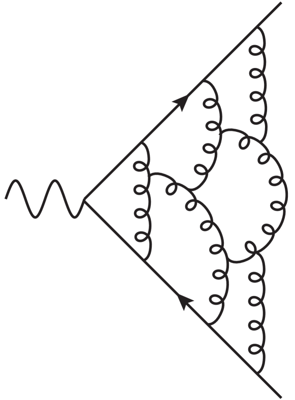
(a)

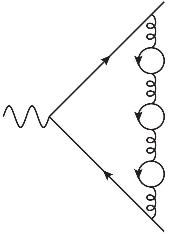
(b)

Figure 1: Examples of Feynman graphs representative of the factorial growth of perturbative coefficients at large orders.

Once again, one may legitimately fear a loss of predictivity, and one may ask – assuming one believes in the consistency of the underlying theory – what was the mistake that lead to the problem. Once again the answers are rich with insights and discoveries: in this case, the underlying assumption was that non-perturbative effects would be negligible, or in some sense decoupled from the perturbative expansion. This, quite interestingly, turns out not to be the case. The factorial growth in the number of diagrams can be precisely related to the existence of non-trivial classical solutions – instantons – which are not accessible by means of a weak-coupling expansion [9, 10]; renormalon singularities, which can be detected by means of fermion-loop chains, reveal contributions to observables originating from vacuum condensates, in many cases matching the results of the operator product expansion [11]. Remarkably, perturbation theory seems to know about its own limitations, and can be used to infer the existence of non-perturbative effects and study their impact. While these insights are several decades old, new powerful techniques are currently being developed to refine existing tools and consolidate their mathematical foundations (see for example [12, 13, 14]).

Finally, we come to the subject of our review. Even after renormalisation, and even if we confine ourselves to perturbative effects, Eq. (1.2) is still ‘wrong’ for most interesting theories with massless particles (and in particular for unbroken gauge theories in $d=4$): expressions for the coefficients $c_{k}(Q/\mu)$ involve integrals that diverge at low energies (in momentum space) or at large distances (in coordinate space). Furthermore, if we attempt to compute the probability for the emission of one or more massless particles in connection with a hard scattering process, this will typically also diverge. This infrared catastrophe was actually the first problem to be clearly identified, among those we have discussed. Long before quantum field theory was fully developed, some of the earliest studies of the interactions of electrons with electromagnetic radiation showed that the frequency spectra of emitted photons behave like $d\nu/\nu$, and thus are not integrable at low frequencies. This emerged from analyses of electron scattering in a Coulomb field, when allowing for extra photon radiation [15, 16], with results subsequently refined in [17], where pair production in the Coulomb field was also considered.

Following the logic we proposed, we may ask one last time what was the mistake that led to this problem. The answer to this question has several layers of depth, that we will explore in the rest of this review, but it is interesting, and truly remarkable, that a precise understanding of the underlying physical problem was developed as early as 1937, with the seminal paper by Bloch and Nordsieck [18]. It is worthwhile to reproduce here the Abstract of that paper, which reads as follows.

Previous methods of treating radiative corrections in non-stationary processes such as the scattering of an electron in an atomic field or the emission of a $\beta$-ray, by an expansion in powers of $e^{2}/\hbar c$, are defective in that they predict infinite low frequency corrections to the transition probabilities. This difficulty can be avoided by a method developed here which is based on the alternative assumption that $e^{2}\omega/mc^{3}$, $\hbar\omega/mc^{2}$ and $\hbar\omega/c\Delta p$ ($\omega=$angular frequency of radiation, $\Delta p=$change in momentum of electron) are small compared to unity. In contrast to the expansion in powers of $e^{2}/\hbar c$, this permits the transition to the classical limit $\hbar=0$. External perturbations on the electron are treated in the Born approximation. It is shown that for frequencies such that the above three parameters are negligible the quantum mechanical calculation yields just the directly reinterpreted results of the classical formulae, namely that the total probability of a given change in the motion of the electron is unaffected by the interaction with radiation, and that the mean number of emitted quanta is infinite in such a way that the mean radiated energy is equal to the energy radiated classically in the corresponding trajectory.

In essence, Bloch and Nordsieck argue that, in the soft photon limit, perturbation theory (in powers of $\alpha=e^{2}/(\hbar c)$) must be abandoned, and they advocate a different approximation scheme (what we now call eikonal approximation), valid when the photon energy is much smaller than the other energy scales in the problem (the electron mass and the momentum trasfer), and the photon wavelength is much larger than the classical electron radius $r_{e}=e^{2}/(mc^{2})$. They then show that this approximation is semiclassical, in that the classical result for the mean radiated energy is recovered, but this entails the radiation of an infinite number of low-energy photons.

The Bloch and Nordsieck paper is truly remarkable because it engineers the cancellation of divergences between virtual corrections and real-radiation contributions, long before the treatment of virtual corrections could be formalised, and furthermore it provides the first example of an all-order summation of perturbation theory. In the following decades, it received several refinements, which proved the complete generality of the results, placed it squarely in the context of (renormalised) QED [19, 20], and significantly streamlined the proof [21]. We will briefly summarise the argument, in modern language, in Section 1.1. We still need, however, to properly diagnose the mistake that lies at the origin of the problem: in this regard, there are two complementary viewpoints.

First, one can argue that the problem is the proper definition of an observable. In a theory with massless particles, in any scattering process one can produce particles with infinitesimal energy, as well as particles with infinitesimal angular separation; on the other hand, every physical detector has finite energy and angular resolutions. Quantum mechanics prescribes that we sum over all configurations we do not observe, so, in principle, an arbitrary number of low-energy or collinear particles must be included in a proper definition of an observable cross section. When this is done, the result is expected to be finite, as it corresponds to a truly measurable quantity. This line of reasoning led to the most general theorem concerning the cancellation of infrared singularities, the KLN theorem [22, 23]. In particular, Ref. [23] shows that the cancellation is a completely general property of any quantum-mechanical system whose Hilbert space contains sets of energy-degenerate states. We will sketch a proof of the KLN theorem in Section 1.2. Before we continue, however, we need to make the argument a little sharper: in principle, the probability for emission of soft or collinear particles could be small, and the effect on the cross section negligible. In order to understand the physics of infrared enhancements, consider a diagram for the emission of a photon from an external fermion leg in massless QED, shown in Fig. 2.

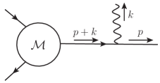
Figure 2: A photon emission diagram in massless QED, possibly responsible for infrared divergences in soft and collinear configurations.

The QED Feynman rules give an expression of the form

$$e\,\overline{u}(p)\,\gamma^{\mu}\frac{\not{p}+\not{k}}{(p+k)^{2}+{\rm i}\eta}\;{\cal M}\,,$$ (1.3)

where ${\cal M}$ represent the rest of the scattering process, which may involve many external legs and virtual corrections as well. If the photon is emitted in the final state, so that $k^{2}=p^{2}=0$, the denominator of the fermion propagator reads $2p\cdot k+{\rm i}\eta=E_{p}\omega_{k}(1-\cos\theta_{pk})+{\rm i}\eta$, where $E_{p}=|{\bf p}|$ and $\omega_{k}=|{\bf k}|$. While the $\eta$ prescription protects from an outright singularity, one must expect enhancements from three sources: the soft photon limit $\omega_{k}\to 0$, the soft fermion limit $E_{p}\to 0$, and the collinear limit $\theta_{pk}\to 0$. Whether these enhancements translate into actual divergences will depend on the specific observable one is computing, and more generally on the theory one is considering. To this end, one will need to develop appropriate power-counting techniques (discussed here in Section 3), similarly to what is done for ultraviolet enhancements; for example, we can anticipate that the soft fermion limit never leads to divergences in renormalisable theories, thanks to an extra power of the energy arising from the wave functions of massless spinors. Note also that, in case the fermion were massive, the collinear singularity would be regulated by the fermion mass, since the angular factor in the denominator would read $(1-|{\bf v}|\cos\theta_{pk})$, with $|{\bf v}|<1$ the velocity of the fermion.

That being said, the origin of the enhancement is apparent: in the limits considered, the fermion propagator reaches the mass shell, $(p+k)^{2}=0$; furthermore, since we are working in covariant perturbation theory, all four momentum components are conserved at each vertex; thus, the intermediate fermion with momentum $p+k$ is a physical state in our theory, and can propagate freely for any length of space and interval of time. When deriving the momentum-space Feynman rules, we have formally integrated over the position of the photon emission vertex in spacetime, under the assumption that emission at long distances should be sufficiently suppressed. Unfortunately, it is not, a consequence of the fact that QED (like all unbroken gauge theories) has long-range interactions. The same conclusion is reached, perhaps in an even more transparent way, if one uses Time-Ordered Perturbation Theory (TOPT) (see, for example, Ref. [2] for a detailed discussion): within that framework, all particles in intermediate states are on the mass shell; energy, on the other hand, is not in general conserved at the vertices, which forces the interactions to take place in a finite time. For soft or collinear emissions, the energy deficit at the emission vertex vanishes, so that once again late-time emissions are unsuppressed. In this sense, both soft and collinear divergences are properly described as long-distance effects.

Importantly, these conclusions are essentially unaffected if the photon line in Fig. 2 folds back and attaches to some other fermion line in the amplitude, forming a loop, instead of being radiated into the final state. In that case, the denominator of the fermion propagator has an additional $k^{2}$, which however is negligible with respect to $p\cdot k$ if all components of the photon momentum become small at the same rate. Clearly, some power counting tools will have to be developed to weigh the presence of the loop integral (as opposed to the phase-space integration over the real photon momentum) and of the photon propagator, but the basic fact remains that, even for virtual corrections, soft and collinear emissions are dangerously enhanced at large distances and times. This provides the seeds for the eventual cancellation of divergences between virtual and real corrections: both are enhanced by the same mechanism, and both must be included to allow for the finite energy and angle resolutions of detectors; once a properly defined observable is constructed, they must, and do, cancel each other.

Let us summarise this first viewpoint on the mistake that led to the rise of infrared divergences, as it emerges from the Bloch-Nordsieck analysis. Theories with massless particles have long-range interactions; as a consequence, late- (and early-) time emissions are not sufficiently suppressed; in the circumstances, our organisation of perturbation theory in powers of the coupling, which distinguishes between virtual corrections and (undetected) real emissions is inadequate, hence individual matrix elements are ill-defined. The proposed solution is to introduce a temporary fix for the matrix elements (an infrared regulator such a particle mass), in the knowledge of the fact that the singular dependence on the regulator will cancel in properly defined observable cross sections.

The second viewpoint on the origin of the infrared problem is the following: when constructing our quantum theory, we have mis-identified the asymptotic states. In most textbook constructions of the $S$-matrix, one finds, somewhere along the way, a statement on the need to assume that interactions can be adiabatically switched off at large times. In theories with massless particles and long-distance interactions, this is simply unrealistic: after a hard interaction, electrons will continue to emit and absorb photons all the way into the asymptotic regime. Choosing as asymptotic states the eigenstates of the free hamiltonian (in QED, Fock states with a fixed number of electrons and photons) is inadequate, as such states are not a good approximation of the actual physical asymptotic states. Indeed, splitting the hamiltonian into ‘free’ and ‘interaction’ terms, as usually done, is inadequate, since interactions persist at late and early times, and such asymptotic interactions should be moved to the part of the hamiltonian that one will attempt to diagonalise exactly. With a better choice of asymptotic states, one may hope not only to improve the algorithm to compute physical observables, but also to rescue the $S$-matrix program, by defining scattering amplitudes that are automatically well-defined, even in the presence of massless particles. This idea was successfully pursued in QED, starting with preliminary studies in Refs. [24, 25, 26, 27, 28, 29], and culminating with the seminal paper by Kulish and Faddeev [30], where a separable, Lorentz- and gauge-invariant Hilbert space of ‘coherent states’ is defined, and the finiteness of the QED $S$-matrix in the coherent state basis is proved to all orders. The coherent state approach will be introduced here in Section 1.3.

Even in the relatively simple case of the abelian theory, understanding our IR mistake has been quite fruitful: the role of long-distance dynamics has been exposed, a sharper definition of a physical observable has emerged, and a more accurate characterisation of asymptotic states has rescued the notion of scattering amplitudes in the presence of massless particles. The generalisation of these ideas to the much more intricate case of non-abelian theories will occupy most of our review. It is to be expected that this generalisation will be far from trivial, given what we know about the long-distance behaviour of unbroken non-abelian gauge theories: perturbative asymptotic states have very little to do with their non-perturbative, confined counterparts, and we can expect and hope that perturbation theory will carry at least some partial information about this breakdown.

Studies of the infrared problem in non-abelian theories started in the mid-seventies [31, 32, 33]. It soon became evident that the simple cancellation mechanism for soft singularities uncovered by Bloch and Nordsieck in QED, which involves only a sum over degenerate final states, does not work for non-abelian theories [34, 35, 36, 37, 38, 39], and a full cancellation can happen only considering degenerate initial states as well. A more general problem arises because collinear divergences, which are regulated by fermion masses in QED, are intrinsic and unavoidable for non-abelian theories, even when matter fields are massive: the three-gluon vertex involves three strictly massless particles and inevitably leads to collinear problems. In the presence of collinear divergences, in particular those associated with radiation from initial-state coloured particles, it is clear from the outset that a simple pattern of cancellation à la Block-Nordsieck cannot work, since hard collinear emissions from the initial state drastically alter the kinematic configuration of the hard scattering, while virtual corrections do not affect it: the cancellation of singularities must therefore be spoiled. At the level of scattering amplitudes, this means that the coherent state program for non-abelian theories is bound to be much more intricate than was the case for QED. Important results were however obtained through the eighties, shedding light on many aspects of the fixed-order and all-order structure of infrared effects, in particular in QCD [46, 47, 48, 49, 50, 51, 52, 53, 54, 55, 56, 57, 58]; these analyses culminated in a formal proof of the finiteness of the non-abelian $S$-matrix in the coeherent-state basis, including the case of collinear divergences, in Ref. [59]. At the level of cross-sections, the problem of initial-state collinear divergences was of course the starting point for the QCD factorisation program, reviewed for example in [60, 61].

More recent studies have focused on two (overlapping) directions. On the one hand, the demands of precision phenomenology have required developing efficient tools for high-order calculations of observable cross sections. In this regard, the coherent state approach, notwithstanding its physical appeal, has not been the main way forward: rather, a ‘KLN’ approach has prevailed, in which virtual corrections and phase-space integrals of unresolved real radiation are both computed with an infrared regulator, and then combined to construct finite distributions. Not surprisingly, dimensional continuation, setting $d=4-2\epsilon$ with $\epsilon<0$, has been the regulator of choice, since it preserves gauge and Lorentz invariance without adding to the complexity of the calculation by introducing non-trivial dependence on unphysical mass scales. Finite-order calculation will be discussed in Section 2, and detailed algorithms for the cancellation of IR poles will be introduced in Section 6.

On the other hand, perhaps more interestingly from a theoretical viewpoint, a great deal of activity has been devoted to elucidate the all-order structure of infrared singularities, on the basis of the ideas of factorisation and universality. In principle, these ideas are natural, and they apply equally well to amplitudes and to cross sections: as we argued, IR singularities are associated with phenomena that take place at large times and distances from the hard scattering center; this suggests that the singularity structure should be largely independent on the details of the short-distance process being considered; one may then hope to identify universal factors responsible for the singular behaviour of the amplitude (or cross section). In practice, proving these properties in a non-abelian theory by standard perturbative methods is very challenging: collinear configurations carry spin correlations between different particles taking part in the scattering, while soft configurations are responsible for very interesting but very intricate colour correlations at large distances. Factorisation emerges only upon summing over Feynman diagrams, and only after the constraints of gauge invariance have been properly taken into account by means of Ward identities. At the level of scattering amplitudes (which will be the focus of most of our discussion) the factorisation program was started with pioneering work on form factors, first in QED [62, 63] and subsequently in QCD [64, 65], with the first extensions to fixed-angle scattering amplitudes coming shortly thereafter [66]. The generalisation of these results to multi-particle scattering amplitudes in the modern language of dimensional regularisation will be the central focus of our review.

In the remainder of this introductory Section, we will present short accounts of the Bloch-Nordsieck cancellation mechanism in QED, of the KLN theorem, and of the coherent state method, with an eye to the long history of the subject, but also to display in some more detail the different underlying viewpoints, that we have just briefly introduced. In Section 2, we will present some well-known one-loop results in QCD, in the modern language of dimensional regularisation: this is textbook material, but it will give us the opportunity to introduce some tools that will be useful in what follows, including in particular the $d$-dimensional running coupling and the calculation of eikonal integrals in dimensional regularisation. In Section 3, we will introduce the methods required to perform an all-order diagrammatic analysis of the IR problem, which are a pre-requisite for the proof of any factorisation theorem. These methods were reviewed in [61], and are presented in much greater detail in [2, 67]; we decided however to include a pedagogical introduction and work out some key examples, since this toolbox lies at the foundation of all subsequent developments. Sections 4 and 5 form the core of our review. First, in Section 4, we consider the case of form factors, and we show how the tools developed in Section 3 lead to the formulation of an all-order factorisation theorem, isolating soft and collinear divergences of form factors in universal functions, which can be defined in terms of gauge-invariant matrix elements of fields and Wilson lines. Once factorisation has been achieved, evolution equations are bound to follow, and solving them leads to an all-order summation of perturbative contributions, in this case of IR poles [68, 69, 70]. Form factors have the advantage of having a trivial colour structure: extending the analysis to general non-abelian scattering amplitudes is therefore less than trivial. This is pursued in Section 5, where the central concept of IR anomalous dimension matrix is introduced, and the most general form of the exponentiation of IR singularities is derived; known results up to three loops for the anomalous dimension matrix are reviewed [71, 72, 73, 74, 75, 76, 77], and the most recent diagrammatic techniques for its calculation are introduced. It is perhaps worthwhile to emphasise that all the results of Sections 4 and 5 are valid not only for QCD, but in fact for any massless gauge theory (with computable corrections in case the gauge fields are coupled to massive matter fields): for example, they have found important application in the case of conformal gauge theories, in particular ${\cal N}=4$ Super-Yang-Mills theory [78, 79]. On the other hand, Sections 4 and 5 focus on virtual corrections to fixed-angle scattering amplitudes, while the construction of measurable cross-sections must also include unresolved soft and collinear real radiation. Factorisation for real radiation is by itself a vast subject, and we don’t do it justice by providing just a brief summary in Section 6; there, we also introduce modern subtraction algorithms [80, 81], which are currently being developed for high-order perturbative calculations [82], in order to perform the cancellation of IR singularities in a general and efficient manner, even for the intricate observables currently being measured at high-energy colliders.

As must be the case when reviewing a broad subject with a long history, many important developments and lines of research that are closely related to our topic were left out: we provide here a partial list, with some of the references that we believe can be useful for further exploration by the reader. First of all, we say very little in this review about the subject of resummation of large logarithms that arise in observable QCD cross sections and that are closely related to infrared singularities (for example threshold logarithms and transverse momentum logarithms): we only note in passing that the techniques used for resummations are tightly connected to the ones reviewed here, which indeed in some cases were developed directly for cross sections before being applied to amplitudes. QCD tools for resummation are reviewed, for example, in Refs. [61, 83, 84], while automated methods are discussed in [85, 86]. Next, we recall that techniques to construct factorisation theorems in QCD, under certain general assumptions, and to derive the corresponding resummations, were made systematic in Refs. [87, 88, 89, 90, 91, 92, 93], by the construction of Soft-Collinear Effective Theory (SCET), a non-local effective field theory for soft and collinear modes of quark and gluon fields. While the bulk of SCET applications concerns cross sections of phenomenological interest, SCET methods are of course fully applicable to the study of scattering amplitudes, and indeed some of the general results discussed here in Section 5 were independently derived within the SCET framework [75, 95]. SCET has generated countless important phenomenological applications, and is introduced and reviewed in Ref. [96]; comparisons between the SCET approach and QCD factorisation were carried out, for example, in Refs. [97, 98, 99, 100, 101, 102, 103, 104]. A third direction that we do not explore is the extension of factorisation theorems, and eventually resummation techniques, beyond leading power in the singular variables (for example the soft gluon energy). In QED, a classic result in this regard is the Low-Burnett-Kroll theorem [105, 106], showing that next-to-leading power (NLP) contributions of soft photons to QED cross section are still universal, as an effect of gauge invariance; the theorem was later extended to collinear-enhanced configurations in Ref. [107]. NLP contributions to amplitudes and cross sections do not induce divergences in renormalisable theories, but they are nevertheless very interesting for both theoretical and phenomenological reasons. In recent years, their factorisation and resummation properties have been studied intensively, both with direct QCD methods (see, for example, Refs. [108, 109, 110, 111, 112, 113, 114, 115, 116]) and in the context of SCET (see, for example, Refs. [91, 117, 118, 119, 120, 121, 122, 123, 124, 125, 126]). A thorough review of these developments together with a survey of recent literature can be found in Ref. [136]. A final important connection that we do not develop here is that between gauge theories and gravity, first discussed in the pioneering work of Weinberg [137]. Similarities and differences between massless gauge theories and gravity theories are intriguing, and have been addressed in the context of factorisation in a number of recent papers [138, 139, 140, 141, 142, 143, 144, 145, 146]. The connection between gauge theories and gravity theories is also at the root of radical re-interpretation of infrared phenomena, which originated in the work of Strominger [147, 148]. Within this framework, infrared divergences are related to infinite-dimensional asymptotic symmetries of the (gauge or gravity) theory under consideration, acting on the celestial sphere intersecting the future (or past) light cone at asymptotic distances. For gravity, these symmetries were uncovered in [149, 150], while for gauge theories they take the form of ‘large’ gauge transformations with non-trivial action at future (or past) null infinity [151, 152, 153, 154, 155, 156, 157, 158, 159, 160]. The universal form of soft and next-to-soft factors for tree-level radiative amplitudes emerges from the Ward identities of these symmetries. Early developments in this fast-developing field are reviewed in [161]. While most of the work done so far within this framework concerns tree-level gravity or gauge-theory amplitudes (see, however, Refs. [162, 163]), the connection between infrared properties of $d=4$ gauge theories and $d=2$ conformal invariance on the celestial sphere is very intriguing, and represents a remarkable new point of view on an old problem. In Section 5, we will see that scale invariance plays an important role for infrared factorisation at any perturbative order: conformal invariance, however, is broken by quantum effects. Furthermore, we will see that the celestial framework allows for a remarkable rephrasing of the all-order expression for infrared-divergent colour-dipole correlations, and indeed an interpretation emerges in terms of a specific two-dimensional conformal theory on the celestial sphere [164]. Further exploration of these ideas in the context of all-order perturbative calculations is undoubtedly of great interest.

As is perhaps evident from this long introduction, the present review has a strong pedagogical emphasis, and we hope that it may help students and junior researchers to gain an orientation in a field with a long history, which however is still quickly progressing in both theoretical and phenomenological directions. At the same time, we have included in Section 5 and in Section 6 some very recent developments, which may be interesting to QCD practitioners, and give a flavour of current research. Possible future directions of research are briefly discussed in Section 7.

1.1 Catastrophe and recovery in QED

In this Section, and in the following Sections 1.2 and 1.3, we take a largely historical perspective, and we present classic results on the cancellation of infrared singularities, which also serve to introduce some of the key concepts to be developed later in the context of non-abelian theories. We begin by looking at the relatively simple case of QED with massive fermions, and we derive the cancellation of soft divergences between virtual correction and final-state real radiation, first at the lowest non-trivial order, and then to all-orders, where one can rather easily demonstrate the exponentiation of the lowest-order result. Our emphasis is on the concepts that will later be developed in greater detail, so the proof that we discuss is heuristic: for a detailed analysis one should refer, for example, to [21]. Rather than using directly the arguments of Ref. [18], we will take advantage of the more modern language of Ref. [137].

Choosing a simple example, which however displays all the general features of the proof, we consider the process where an electron scatters from another heavy particle by means of $t$-channel photon exchange. The heavy particle simply plays the role of a source for an external photon field. We will first show the cancellation at one loop, and then discuss how the mechanism generalises to all orders.

At order $\alpha$, the diagrams contributing to virtual corrections are shown in Fig. 3, while those contributing to real photon radiation (bremsstralung) are shown in Figure 4.

(a)

(b)

(c)

(d)

Figure 3: Virtual corrections to electron scattering from a heavy particle, at order $\alpha$.

(a)

(b)

Figure 4: Bremsstrahlung diagrams for electron scattering from a heavy particle, contributing to the cross section at order $\alpha$.

We begin by considering the differential cross-section for radiating a photon with momentum $k$, when the electron scatters from a state of momentum $p$ to a state of momentum $p^{\prime}$, assuming $k^{\mu}\ll q^{\mu}\equiv(p^{\prime}-p)^{\mu}$. The matrix element for this process is the sum of two terms of the form depicted in Fig. 2, and greatly simplifies when one expands in powers of the soft momentum $k$ and considers only the leading power (this soft approximation will be considered in greater detail in Section 2.6 and in Section 3.3). At this order, referring to Eq. (1.3) but appropriately introducing the electron mass, one can perform the following manipulations:

• neglect $k$ in the numerator;

• neglect $k^{2}$ in the denominator;

• commute the hard momentum factor $p\hskip-4.49997pt/$ (or $p\hskip-4.49997pt/^{\prime}$) in the numerator of the electron propagator across the emission vertex, and use the Dirac equation to simplify the expression.

Contracting the result with the photon polarisation vector $\varepsilon(k)$, and denoting the lowest-order matrix element by ${\cal M}_{0}$, the leading power result for the radiative matrix element ${\cal M}_{\rm rad}$ takes the form

$${\cal M}_{\rm rad}\,=\,e\,\bigg{(}\frac{p^{\prime}\cdot\varepsilon(k)}{p^{\prime}\cdot k}-\frac{p\cdot\varepsilon(k)}{p\cdot k}\bigg{)}\,{\cal M}_{0}\,,$$ (1.4)

where $e$ is the electron charge. The soft approximation in Eq. (1.4) has several remarkable properties that we will explore later. Here we simply note that it is gauge invariant (it vanishes for longitudinally polarised photons), independent of the spin of the emitter and singular – as expected – for small $k$. It is formally easy to construct a soft approximation for the total radiative cross section: at leading power in $k$ the phase space factorises, and the flux factor reduces to the flux factor for the non-radiative process. Summing over polarisations, we find that the cross section for the radiation of a single real soft photon is given by

$$\sigma_{r}\big{(}e(p)\rightarrow e(p^{\prime})+\gamma\big{)}\,=\,\sigma_{0}\big{(}e(p)\rightarrow e(p^{\prime})\big{)}\,\,{\cal I}_{r}\bigg{(}\frac{m^{2}}{q^{2}},\frac{\mu^{2}}{E^{2}},\epsilon\bigg{)}\,,$$ (1.5)

where we defined the soft factor for real radiation, ${\cal I}_{r}$, by

$${\cal I}_{r}\bigg{(}\frac{m^{2}}{q^{2}},\frac{\mu^{2}}{E^{2}},\epsilon\bigg{)}\,=\,-\frac{e^{2}(2\pi\mu)^{2\epsilon}}{16\pi^{3}}\!\int_{0}^{E}d|{\bf k}||{\bf k}|^{1-2\epsilon}\!\int d\Omega_{2-2\epsilon}\bigg{(}\frac{p^{\prime\mu}}{p^{\prime}\cdot k}-\frac{p^{\mu}}{p\cdot k}\bigg{)}\bigg{(}\frac{p^{\prime}_{\mu}}{p^{\prime}\cdot k}-\frac{p_{\mu}}{p\cdot k}\bigg{)}\,.$$ (1.6)

In Eq. (1.6) we have introduced dimensional regularisation, setting $d=4-2\epsilon$, $\epsilon<0$, since the integral is ill-defined in $d=4$, diverging logarithmically as $|{\bf k}|\rightarrow 0$: this is the original infrared catastrophe of Ref. [18]. The fact that the divergence is logarithmic justifies a posteriori our choice to retain only the leading power in the soft expansion: sub-leading terms will contribute finite corrections. Furthermore, we integrate over photon energies up to an arbitrary cutoff $E\ll\sqrt{-q^{2}}$, which represents the minimum energy resolution of our detector: photons with $|{\bf k}|<E$ are unresolved, and their contribution must be included. The resulting integral is well known and not difficult to compute. One finds

$${\cal I}_{r}\bigg{(}\frac{m^{2}}{q^{2}},\frac{\mu^{2}}{E^{2}},\epsilon\bigg{)}\,=\,-\,\frac{\alpha}{\pi}\,\frac{1}{\epsilon}\bigg{(}\frac{4\pi{\mu}^{2}}{E^{2}}\bigg{)}^{\epsilon}\left[\left(\frac{1-2m^{2}/q^{2}}{\beta}\right)\log\frac{\beta+1}{\beta-1}-1\right]+{\cal O}\big{(}\epsilon^{0}\big{)}\,,$$ (1.7)

where

$$\beta\,=\,\sqrt{1-4m^{2}/q^{2}}\,>\,1\,.$$ (1.8)

It is interesting to consider explicitly the limit of large momentum transfer, $-q^{2}\rightarrow\infty$, focusing on terms enhanced by logarithms of $q^{2}$. We obtain

$${\cal I}_{r}\bigg{(}\frac{m^{2}}{q^{2}},\frac{\mu^{2}}{E^{2}},\epsilon\bigg{)}\,\simeq\,\frac{\alpha}{\pi}\left[-\frac{1}{\epsilon}\log\left(\frac{-q^{2}}{m^{2}}\right)+\log\left(\frac{E^{2}}{4\pi\mu^{2}}\right)\log\left(\frac{-q^{2}}{m^{2}}\right)\right]\,.$$ (1.9)

As we will see, the soft pole in $\epsilon$ will cancel against the virtual correction; the second term displays the characteristic ‘Sudakov’ double-logarithmic enhancement, with one logarithm of soft origin (here parametrised by the resolution scale $E$) and one logarithm of collinear origin (which becomes a divergence in the massless limit, $m\to 0$).

Let us now turn to the evaluation of virtual corrections. The problem is significantly more intricate because of the concurrent presence of ultraviolet divergences, which must be dealt with by means of renormalisation: in particular, one must make sure that no infrared divergences survive in the UV counterterms appropriate to the chosen renormalisation scheme. This can be achieved for example by using a minimal scheme. On the other hand, in the on-shell scheme typically used in QED, both the electron field renormalisation constant $Z_{\psi}$ and the vertex renormalisation constant $Z_{1}$ contain IR divergences, which however cancel in the scattering amplitude thanks to the QED Ward identity [2]. Armed with this preliminary result, we can concentrate on the vertex correction diagram of Fig. 3(a), which, as we will see, gives the only surviving infrared-singular contribution. A straightforward power-counting argument shows that only terms with no powers of the photon momentum in the numerator can give infrared singularities, and those will be logarithmic. In this approximation, diagram (a) in Fig. 3 gives

$$(a)_{\rm soft}\,=\,-\,e^{3}\mu^{3\epsilon}\int\frac{d^{d}k}{(2\pi)^{d}}\frac{\overline{u}(p^{\prime})\gamma^{\alpha}(\not{p}^{\prime}+m)\gamma^{\mu}(\not{p}+m)\gamma_{\alpha}u(p)}{(k^{2}+{\rm i}\eta)(k^{2}-2p^{\prime}\cdot k+{\rm i}\eta)(k^{2}-2p\cdot k+{\rm i}\eta)}\,.$$ (1.10)

The integral in Eq. (1.10) can be performed with standard methods, yielding a single infrared pole in $\epsilon$: potentially, a second infrared catastrophe. Instead of directly computing the integral, in view of the generalisation to higher orders, it is more instructive to take the soft approximation further, and perform on the integrand the same steps that we applied to the real emission diagrams, i.e. neglecting $k^{2}$ in the denominator, and using the Dirac equation to simplify the numerator. Recognising that the lowest-order matrix element factorises, we write then

$$(a)_{\rm soft}\,=\,\big{(}{\rm i}e^{2}\mu^{2\epsilon}\big{)}\,{\cal M}_{0}\int\frac{d^{d}k}{(2\pi)^{d}}\frac{p\cdot p^{\prime}}{(k^{2}+{\rm i}\eta)(-p^{\prime}\cdot k+{\rm i}\eta)(-p\cdot k+{\rm i}\eta)}\,.$$ (1.11)

We note that the step between Eq. (1.10) and Eq. (1.11) has apparently generated a new problem: the integral in Eq. (1.11) is now also divergent in the UV, a region where our approximation breaks down. This UV singularity is not present in the original QED calculation: it is a singularity of a low-energy effective theory for the infrared sector of QED, and it will be of great interest for the developments discussed in Section 4. For the moment, we will simply introduce a UV regulator and focus on the infrared pole.

Examining Eq. (1.11), one begins to see some similarities with the integral in Eq. (1.6): these can be sharpened by taking two further steps. First of all, we include the UV counterterms appropriate to the original QED calculation, picking the on-shell renormalisation scheme, which makes the calculation particularly transparent. In the on-shell scheme, the self-energy counterterm for the graphs in Fig. 3(b) and 3(c) is such that the sum of the graph plus the counterterm vanishes on shell: these graphs therefore do not contribute to our calculation. The vertex counterterm, on the other hand, is fixed by the requirement that the renormalised vertex correction vanish for $q^{2}=0$, i.e. for $p^{\prime}=p$. This can be enforced directly in our soft approximation by writing [2]

$$(a+{\rm counterterm})_{\rm soft} = {\cal M}_{0}\,\,\bigg{(}\!\!-\frac{{\rm i}e^{2}\mu^{2\epsilon}}{2}\bigg{)}\int\frac{d^{d}k}{(2\pi)^{d}}\frac{1}{(k^{2}+{\rm i}\eta)}\left(\frac{p^{\prime\mu}}{-p^{\prime}\cdot k+{\rm i}\eta}-\frac{p^{\mu}}{-p\cdot k+{\rm i}\eta}\right)^{2}$$ (1.12)

$$\equiv {\cal M}_{0}\,\,{\cal I}_{v}\bigg{(}\frac{m^{2}}{q^{2}},\frac{\mu^{2}}{q^{2}},\epsilon\bigg{)}\,,$$

which manifestly vanishes for $p^{\prime}=p$, and where the cross term in the square of the parenthesis gives Eq. (1.11), while the squares of the two terms (which depend only on $m^{2}$) give the counterterm. The final step to bring Eq. (1.12) to a form directly comparable to Eq. (1.6) is to note (following Ref. [137]) that the real part of the integral ${\cal I}_{v}$ has support only on the photon mass shell, $k^{2}=0$. This can be seen by focusing on the $k_{0}$ integration, and observing the locations of the poles in the $k_{0}$ complex plane in Eq. (1.11): the poles associated with the fermion lines are in the upper-half plane, as is one of the two poles associated with the photon propagator. One can therefore compute the integral by closing the contour in the lower-half plane, and picking the residue of the photon pole, which effectively places the photon on the mass shell. The result is now precisely of the form of Eq. (1.6), except for an overall factor of $-1/2$, and the fact that the resolution parameter $E$ must be replaced with an ultraviolet cutoff, which can naturally be chosen as $\sqrt{-q^{2}}$. We have then

$${\cal I}_{v}\bigg{(}\frac{m^{2}}{q^{2}},\frac{\mu^{2}}{q^{2}},\epsilon\bigg{)}\,=\,-\frac{1}{2}\,{\cal I}_{r}\bigg{(}\frac{m^{2}}{q^{2}},\frac{\mu^{2}}{-q^{2}},\epsilon\bigg{)}\,.$$ (1.13)

The observed physical cross section is obtained by summing the real-emission cross section in Eq. (1.5), which gives the leading-order probability for the emission of an undetected soft photon, with the virtual correction to the elastic scattering process, which is proportional to the tree-level cross section, with a factor given by twice the real part of ${\cal I}_{v}$. One finds

$$\sigma_{\rm obs}\big{(}e(p)\rightarrow e(p^{\prime})\big{)}\,=\,\sigma_{0}\big{(}e(p)\rightarrow e(p^{\prime})\big{)}\bigg{[}1+{\cal I}_{r}\bigg{(}\frac{m^{2}}{q^{2}},\frac{\mu^{2}}{E^{2}},\epsilon\bigg{)}+2\,{\cal I}_{v}\bigg{(}\frac{m^{2}}{q^{2}},\frac{\mu^{2}}{q^{2}},\epsilon\bigg{)}\bigg{]}\,.$$ (1.14)

Using Eq. (1.13), we see that all singular terms as $\epsilon\to 0$ cancel, as announced, leaving behind finite logarithms. In the limit of large negative $q^{2}$, for example, the result is

$$\sigma_{\rm obs}\big{(}e(p)\rightarrow e(p^{\prime})\big{)}\,\simeq\,\sigma_{0}\big{(}e(p)\rightarrow e(p^{\prime})\big{)}\left[1-\frac{\alpha}{\pi}\log\left(\frac{-q^{2}}{E^{2}}\right)\log\left(\frac{-q^{2}}{m^{2}}\right)+\mathcal{O}({\alpha}^{2})\right]\,,$$ (1.15)

displaying the product of a soft logarithm and a collinear logarithm. It is appealing that the cancellation we have observed is made possible by the fact that the divergent part of the loop integral originates from configurations in which the virtual photon is on-shell: this resonates with the qualitative arguments given in the Introduction, identifying infrared divergences as long-distance effects. We note however that the correction we find in Eq. (1.15) is finite but negative, and it can lead to a negative cross section at very large momentum transfer. It is clear that the recovery from the IR catastrophe at NLO is only a partial solution, and we need to explore higher-order corrections.

A general and detailed proof of the cancellation of infrared divergences in QED would require developing power-counting tools (discussed here in Section 3), and analysing the impact of renormalisation to all orders [20, 21]. Fortunately, it is possible to understand the general pattern of the cancellation with simple diagrammatic and combinatorial arguments, discussed for example in [137], which are sufficient to deal with terms with the largest logarithmic enhancements at each order of perturbation theory. These tools will provide us with a first glimpse of two essential features of infrared enhancements, factorisation and exponentiation, which will be discussed at length in later Sections.

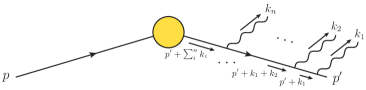
Figure 5: Emission of $n$ photons attached to outgoing electron line.

Consider first the emission of $n$ photons with momenta $k_{1},\ldots,k_{n}$ and polarisation vectors $\varepsilon_{1},\ldots,\varepsilon_{n}$, attached to the outgoing electron line carrying momentum $p^{\prime}$, as depicted in Fig. 5. The contribution to the transition amplitude from this graph is given by

$$G\big{(}1,\ldots,n;p^{\prime}\big{)}\,=\,e^{n}\,\overline{u}(p^{\prime})\,\varepsilon\hskip-4.49997pt/_{1}\,\frac{p\hskip-4.49997pt/^{\prime}+k\hskip-4.49997pt/_{1}+m}{2p^{\prime}\cdot k_{1}}\,\ldots\,\varepsilon\hskip-4.49997pt/_{n}\,\frac{p\hskip-4.49997pt/^{\prime}+k\hskip-4.49997pt/_{1}\ldots k\hskip-4.49997pt/_{n}+m}{2p^{\prime}\cdot\big{(}k_{1}+\ldots+k_{n}\big{)}}\,{\cal H}\,,$$ (1.16)

where ${\cal H}$ is the hard scattering subgraph represented by the circle in Fig. 5. At leading power in each gluon momentum, we can iterate the procedure applied to the single-radiative amplitude, dropping all dependence on $k_{i}$ in the numerator, and repeatedly using the Dirac equation after commuting the electron momentum $p^{\prime}$ to the left. This leads to

$$G\big{(}1,\ldots,n;p^{\prime}\big{)}\,\simeq\,e^{n}\,\,\frac{p^{\prime}\cdot\varepsilon_{1}}{p^{\prime}\cdot k_{1}}\,\frac{p^{\prime}\cdot\varepsilon_{2}}{p^{\prime}\cdot\big{(}k_{1}+k_{2}\big{)}}\,\ldots\,\frac{p^{\prime}\cdot\varepsilon_{n}}{p^{\prime}\cdot\big{(}k_{1}+k_{2}+\ldots+k_{n}\big{)}}\,{\cal M}\,,$$ (1.17)

where the outgoing electron spinor has been reabsorbed in ${\cal M}$, the fixed-order matrix element without photon radiation. Crucially, the contribution to the physical amplitude where $n$ photons are radiated from the outgoing electron line is obtained by summing over $n!$ permutations of the photon lines. Bose symmetry then requires that the result be symmetric under permutations of the photon labels: this happens as a consequence of the eikonal identity

$$\sum_{\sigma}\Bigg{[}\prod_{i=1}^{n}\frac{1}{p\cdot\sum_{j=1}^{i}k_{\sigma(j)}}\Bigg{]}\,=\,\prod_{i=1}^{n}\,\frac{1}{p\cdot k_{i}}\,\,,$$ (1.18)

where $\sigma$ enumerates photon permutations. The identity is easily verified for $n=2$, and can subsequently be proved by induction. It leads to

$$\sum_{\sigma}G\big{(}\sigma(1),\ldots,\sigma(n);p^{\prime}\big{)}\,\simeq\,e^{n}\,\,\prod_{i=1}^{n}\,\frac{p^{\prime}\cdot\varepsilon_{i}}{p^{\prime}\cdot k_{i}}\,{\cal M}\,,$$ (1.19)

representing the uncorrelated emissions of $n$ soft photons without recoil. Notice that soft divergences will arise from the phase-space integration of the emitted photon momenta in Eq. (1.16) only if no hard photons are emitted further out along the electron line, closer to the outgoing electron spinor: any such emission would move all propagators closer to the hard scattering off their mass shell, so that the approximation leading to Eq. (1.16) would not be applicable. We conclude that soft divergences arise from real photon emission only when photons attach to external lines, defined as lines connected to the external states from which every emission is soft: that is why we have factorised the non-radiative matrix element ${\cal M}$ in Eq. (1.19), rather than its tree-level approximation ${\cal M}_{0}$. In a space-time picture, this factorisation of ‘external line’ contributions nicely matches our understanding of soft divergences as long-distance phenomena, and it provides a first example of more intricate factorisation theorems to be discussed in later Sections.

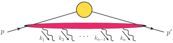
Figure 6: Emission of $n$ photons connected in any order to the initial and final electron lines.

Naturally, an identical argument applies to the incoming electron line, where however each photon contributes with a relative minus sign, since $(p-\Sigma_{i}{k_{i}})^{2}-m^{2}=-2p\cdot\Sigma_{i}{k_{i}}$. Considering together all the diagrams containing $n$ soft photons, connected in any possible order to the incoming and outgoing electron lines, as shown in Fig. 6, we find that each photon contributes precisely an eikonal factor, as was the case in Eq. (1.4). The result is then

$${\cal M}_{\rm rad}^{(n)}\,=\,e^{n}\,\prod_{i=1}^{n}\bigg{(}\frac{p^{\prime}\cdot\varepsilon_{i}}{p^{\prime}\cdot k_{i}}-\frac{p\cdot\varepsilon_{i}}{p\cdot k_{i}}\bigg{)}\,{\cal M}\,.$$ (1.20)

At leading power in each photon momentum $k_{i}$, the phase space for real radiation factorises into a product of phase spaces for individual photons; furthermore, the phase-space integral must include a factor of $1/n!$ for $n$ identical bosons. Summing over polarisations one finds

$$\sigma_{r}^{(n)}\big{(}e(p)\rightarrow e(p^{\prime})+n\gamma\big{)}\,=\,\sigma_{0}\big{(}e(p)\rightarrow e(p^{\prime})\big{)}\,\,\frac{1}{n!}\left[{\cal I}_{r}\bigg{(}\frac{m^{2}}{q^{2}},\frac{\mu^{2}}{E^{2}},\epsilon\bigg{)}\right]^{n}\,,$$ (1.21)

It is now straightforward to sum the series in Eq. (1.21) over the number of soft photons $n$, which results in exponentiation of the single-photon result,

$$\sigma_{r}\big{(}e(p)\rightarrow e(p^{\prime})\big{)}\,=\,\sigma_{0}\big{(}e(p)\rightarrow e(p^{\prime})\big{)}\,\exp\Bigg{[}\,{\cal I}_{r}\bigg{(}\frac{m^{2}}{q^{2}},\frac{\mu^{2}}{E^{2}},\epsilon\bigg{)}\Bigg{]}\,.$$ (1.22)

We can now observe that most of the steps leading to Eq. (1.22) also apply to virtual corrections: only combinatorial factors must be carefully considered. First of all, only virtual photons attaching to external lines will generate soft divergences. Next, focusing on vertex corrections, i.e. on photons connecting the two electron lines, one may apply the eikonal identity in Eq. (1.18), by simply considering $n!$ copies of all diagrams contributing to the $n$-photon vertex correction, and relabelling the photon momenta in each copy: one must then divide the result by $n!$. Notice that one needs to perform this sum and normalisation on only one of the two electron lines, since repeating the operation on the second electron line would reproduce the same diagrams. This step leads to a product of factors of the form of Eq. (1.11). Self-energy corrections on each electron line can then be renormalised to vanish on-shell, and the condition that the vertex correction should vanish at $q^{2}=0$ turns each eikonal factor in the vertex into the form of Eq. (1.12), introducing the appropriate factor of $1/2$ for each photon. We conclude that virtual corrections also exponentiate, and

$$\sigma_{v}\big{(}e(p)\rightarrow e(p^{\prime})\big{)}\,=\,\sigma_{0}\big{(}e(p)\rightarrow e(p^{\prime})\big{)}\,\exp\Bigg{[}\,2\,{\cal I}_{v}\bigg{(}\frac{m^{2}}{q^{2}},\frac{\mu^{2}}{q^{2}},\epsilon\bigg{)}\Bigg{]}\,.$$ (1.23)

Combining real and virtual corrections, we see that, thanks to Eq. (1.13), the cancellation of soft singularities is replicated to all orders in perturbation theory, and one finds

$$\sigma_{\rm obs}\big{(}e(p)\rightarrow e(p^{\prime})\big{)} = \sigma_{0}\big{(}e(p)\rightarrow e(p^{\prime})\big{)}\,\exp\bigg{[}{\cal I}_{r}\bigg{(}\frac{m^{2}}{q^{2}},\frac{\mu^{2}}{E^{2}},\epsilon\bigg{)}+2\,{\cal I}_{v}\bigg{(}\frac{m^{2}}{q^{2}},\frac{\mu^{2}}{q^{2}},\epsilon\bigg{)}\bigg{]}$$ (1.24)

$$\simeq \sigma_{0}\big{(}e(p)\rightarrow e(p^{\prime})\big{)}\,\exp\bigg{[}\!-\frac{\alpha}{\pi}\log\left(\frac{-q^{2}}{E^{2}}\right)\log\left(\frac{-q^{2}}{m^{2}}\right)\bigg{]}\,,$$

where in the second line we have reported the leading double-logarithmic behaviour in the limit of large momentum transfer. Upon combining real and virtual corrrections, and resumming the perturbative expansion, we achieved a finite and well-behaved result: the cross section is positive definite, and it exhibits the classic ‘Sudakov’ behaviour [62], vanishing exponentially at large momentum transfer, or equivalently for small values of the resolution parameter $E$ and of the fermion mass $m$.

1.2 Observable cross sections are finite: the KLN theorem

We have seen that in quantum electrodynamics soft divergences cancel out order by order in perturbation theory, when the transition rates are summed over final states that are physically indistinguishable. From the derivation in Section 1.1, it is not however clear how general the mechanism is, and indeed the cancellation may appear fortuitous. As a matter of fact, as briefly discussed in the Introduction, the Bloch-Nordsieck theorem is specific to QED, and breaks down for non-abelian gauge theories [34, 35, 36, 37, 38, 40, 41]. It is important, therefore, to develop a more general understanding of the cancellation, as well as a more intuitive picture of the underlying physical mechanism. The framework is provided by two general results, known respectively as the Kinoshita-Poggio-Quinn (KPQ) theorem [31, 32, 33] and the Kinoshita-Lee-Nauenberg (KLN) theorem [22, 23, 165, 166], which apply directly to any quantum theory with massless particles. The KPQ theorem establishes that momentum-space Green functions with external momenta which are off the mass shell are infrared safe. This is a natural consequence of the physical picture that we have been developing: the fluctuations of off-shell fields are confined to limited volumes of space-time, and cannot be affected by long-distance singularities. The KLN theorem, on the other hand, establishes the general framework for the cancellation of singularities when on-shell quantities are evaluated: one finds that, in any theory involving massless particles, infrared divergences can be traced to the presence of sets of quantum states that are degenerate in energy, and the divergences cancel when the transition rates are summed over the sets of degenerate initial and final states. In what follows, we will sketch a proof of the KLN theorem, following the line of argument presented in [23]. We find this approach particularly suited to show the complete generality of the cancellation, which indeed applies to any quantum system with sets of states which are degenerate in energy, including non-relativistic theories and effective field theories.

Consider then a quantum-mechanical system, characterised by a Hilbert space of states $\mathcal{H}$, and by a quantum hamiltonian $H$ which we split into a solvable, quadratic part, and an interaction term, as

$$H(t)\,=\,H_{0}+H_{I}(t)\,,$$ (1.25)

Crucially, we work in the interaction picture, where operators evolve in time by the action of the free hamiltonian $H_{0}$, while the time evolution of quantum states is dictated by the interaction hamiltonian $H_{I}(t)$. The time evolution operator is then given by

$$U\big{(}t_{2},t_{1}\big{)}\,=\,{\rm T}\exp\left[-{\rm i}\int_{t_{1}}^{t_{2}}dt\,H_{I}(t)\right]\,,$$ (1.26)

where $H_{I}(t)$ is the interaction hamiltonian in the interaction picture,

$$H_{I}(t)\,=\,{\rm e}^{{\rm i}H_{0}t}\,H_{I}(0)\,{\rm e}^{-{\rm i}H_{0}t}\,.$$ (1.27)

The $S$-matrix of the theory can then be formally defined by the limit

$$S\,\equiv\,\lim_{t,t^{\prime}\to\infty}U(t^{\prime},0)\,U(0,-t)\,\equiv\,\Omega_{-}^{\dagger}\,\Omega_{+}\,,$$ (1.28)

where the $\Omega_{\pm}$ operators, sometimes called Möller operators, are in turn defined by

$$\Omega_{\pm}\,\equiv\,\lim_{t\to\infty}\,T\exp\left[-{\rm i}\int_{\mp t}^{0}dt\,H_{I}(t)\right]\,.$$ (1.29)

Armed with this definition, we can compute transition amplitudes between incoming and outgoing states in terms of the Möller operators, as

$$\big{\langle}b,{\rm out}\big{|}a,{\rm in}\big{\rangle}\,\equiv\,\big{\langle}b,{\rm in}\big{|}\,S\,\big{|}a,{\rm in}\big{\rangle}\,=\,\sum_{c}\big{\langle}b\big{|}\,\Omega_{-}^{\dagger}\,\big{|}c\big{\rangle}\big{\langle}c\big{|}\,\Omega_{+}\,\big{|}a\big{\rangle}\,,$$ (1.30)

where we used the completeness of the incoming states, and, in the last expression, we omitted for simplicity the initial-state label, as we will do in the following. We are tacitly assuming that the asymptotic states are eigenstates of the free hamiltonian $H_{0}$: if there are sets of energy-degenerate states, this is in general not a good approximation (as we will see in detail in the next section), since energy degeneracy signals long-range interactions. In the present setting, the problem emerges in the form of singularities in perturbation theory, which we will have to try to cancel. In order to proceed, we define the transition probabilities (per unit volume and per unit time)

$$P\big{(}a\to b\big{)}\,=\,\big{|}\left\langle\smash{b}{\vphantom{1}}\right|S\left|\smash{a}{\vphantom{1}}\right\rangle\big{|}^{2} = \sum\limits_{c,d}\left(\left\langle\smash{b}{\vphantom{1}}\right|\Omega_{-}^{\dagger}\left|\smash{c}{\vphantom{1}}\right\rangle\left\langle\smash{c}{\vphantom{1}}\right|\Omega_{+}\left|\smash{a}{\vphantom{1}}\right\rangle\right)\left(\left\langle\smash{b}{\vphantom{1}}\right|\Omega_{-}^{\dagger}\left|\smash{d}{\vphantom{1}}\right\rangle\left\langle\smash{d}{\vphantom{1}}\right|\Omega_{+}\left|\smash{a}{\vphantom{1}}\right\rangle\right)^{*}$$ (1.31)

$$= \sum\limits_{c,d}\left\langle\smash{d}{\vphantom{1}}\right|\Omega_{+}\left|\smash{a}{\vphantom{1}}\right\rangle^{*}\left\langle\smash{c}{\vphantom{1}}\right|\Omega_{+}\left|\smash{a}{\vphantom{1}}\right\rangle\left\langle\smash{b}{\vphantom{1}}\right|\Omega_{-}^{\dagger}\left|\smash{c}{\vphantom{1}}\right\rangle\left\langle\smash{b}{\vphantom{1}}\right|\Omega_{-}^{\dagger}\left|\smash{d}{\vphantom{1}}\right\rangle^{*}$$

$$\equiv \sum\limits_{c,d}W_{a,cd}^{+}\left(W_{b,cd}^{-}\right)^{*}\,,$$

where in the last equality we defined the matrices

$$W_{l,cd}^{\pm}\,\equiv\,\left\langle\smash{d}{\vphantom{1}}\right|\Omega_{\pm}\left|\smash{l}{\vphantom{1}}\right\rangle^{*}\left\langle\smash{c}{\vphantom{1}}\right|\Omega_{\pm}\left|\smash{l}{\vphantom{1}}\right\rangle\,,$$ (1.32)

providing a factorisation of the transition rate into two parts, carrying the dependence on the initial state $\left|\smash{a}{\vphantom{1}}\right\rangle$, and on the final state $\left|\smash{b}{\vphantom{1}}\right\rangle$, respectively.

The KLN theorem can be stated in terms of the transition probabilities $P(a\to b)$ as follows. Consider the eigenstates $\left|\smash{\alpha}{\vphantom{1}}\right\rangle$ of the hamiltonian $H$, and let $E_{\alpha}$ be their energies. Focus on the set of eigenstates with energies falling in a fixed interval $E_{0}-\epsilon<E_{\alpha}<E_{0}+\epsilon$, and denote that set by $D_{\epsilon}(E_{0})$. Transition probabilities $P(\alpha\to\beta)$ are in general singular in perturbation theory if $E_{\alpha}$ or $E_{\beta}$ are degenerate. In such cases, one must introduce a regulator for the singularity, for example a mass $m$ for all particles involved in the scattering. In the presence of the regulator $m$, one can then construct the inclusive transition probability

$$P_{m}\Big{[}D_{\epsilon}(E_{a})\to D_{\epsilon}(E_{b})\Big{]}\,\equiv\,\sum\limits_{a\in D_{\epsilon}(E_{a})}\sum\limits_{b\in D_{\epsilon}(E_{b})}P_{m}(a\to b)\,,$$ (1.33)

and the theorem states that this quantity remains finite order by order in perturbation theory when the regulator is removed by taking $m\to 0$. Given Eq. (1.31), this can be proved by considering the matrices $W_{l,cd}^{\pm}$, and showing that the combination

$$\sum\limits_{a\in D_{\epsilon}(E_{a})}W^{\pm}_{a,cd}\,\equiv\,W^{\pm}_{cd}(a)$$ (1.34)

is finite. In order to see how the cancellation comes about, let us begin by considering the first non-trivial perturbative order. Expanding Eq. (1.29) to first order in $H_{I}$ we find, for example

$$\left\langle\smash{i}{\vphantom{1}}\right|\Omega_{-}\left|\smash{j}{\vphantom{1}}\right\rangle = \left\langle\smash{i}{\vphantom{1}}\right|\left[1-{\rm i}\int_{\infty}^{0}dt\,H_{I}(t)\right]\left|\smash{j}{\vphantom{1}}\right\rangle$$ (1.35)

$$= \delta_{ij}+{\rm i}\!\int_{0}^{\infty}dt\left\langle\smash{i}{\vphantom{1}}\right|{\rm e}^{{\rm i}H_{0}t}\,H_{I}{\rm e}^{-{\rm i}H_{0}t}\left|\smash{j}{\vphantom{1}}\right\rangle$$

$$= \delta_{ij}+{\rm i}\left\langle\smash{i}{\vphantom{1}}\right|H_{I}\left|\smash{j}{\vphantom{1}}\right\rangle\int_{0}^{\infty}\!dt\,{\rm e}^{{\rm i}\big{[}\left(E_{i}-E_{j}\right)+{\rm i}\epsilon\big{]}t}$$

$$= \delta_{ij}-\frac{\left\langle\smash{i}{\vphantom{1}}\right|H_{I}\left|\smash{j}{\vphantom{1}}\right\rangle}{E_{i}-E_{j}+{\rm i}\epsilon}\,,$$

where the infinitesimal real constant $\epsilon$ ensures the convergence of the integral at infinity, and $E_{i}$ and $E_{j}$ are the eigenvalues of $H_{0}$ for the states $\left|\smash{i}{\vphantom{1}}\right\rangle$ and $\left|\smash{j}{\vphantom{1}}\right\rangle$, respectively. Eq. (1.35), and the analogous result for the matrix elements of $\Omega_{+}$, can be substituted in Eq. (1.32), yielding

$$W^{\pm}_{a,ij}\,=\,\delta_{ia}\delta_{ja}-\frac{\left\langle\smash{i}{\vphantom{1}}\right|H_{I}\left|\smash{a}{\vphantom{1}}\right\rangle}{E_{i}-E_{a}\mp{\rm i}\epsilon}\,\delta_{ja}-\frac{\left\langle\smash{j}{\vphantom{1}}\right|H_{I}\left|\smash{a}{\vphantom{1}}\right\rangle^{*}}{E_{j}-E_{a}\pm{\rm i}\epsilon}\,\delta_{ia}\,,$$ (1.36)

up to corrections of second order in $H_{I}$. If the energy levels $E_{i}$ and $E_{j}$ become degenerate when the regulator $m$ is removed, Eq. (1.36) exhibits singularities whenever $\left|\smash{a}{\vphantom{1}}\right\rangle$ coincides with either $\left|\smash{i}{\vphantom{1}}\right\rangle$ or $\left|\smash{j}{\vphantom{1}}\right\rangle$. It is easy to verify that the singularities cancel at this order in the combination $W^{\pm}_{cd}(a)$ defined in Eq. (1.34). Four different cases arise naturally

• Both states $\left|\smash{i}{\vphantom{1}}\right\rangle$ and $\left|\smash{j}{\vphantom{1}}\right\rangle$ lie in $D_{\epsilon}(E_{a})$. This is the potentially singular case, but one easily verifies that the contribution with $\left|\smash{a}{\vphantom{1}}\right\rangle=\left|\smash{i}{\vphantom{1}}\right\rangle$ cancels the one with $\left|\smash{a}{\vphantom{1}}\right\rangle=\left|\smash{j}{\vphantom{1}}\right\rangle$. So long as $\left|\smash{i}{\vphantom{1}}\right\rangle\neq\left|\smash{j}{\vphantom{1}}\right\rangle$, one then finds $W_{ij}^{\pm}(a)=0$.

• Only state $\left|\smash{i}{\vphantom{1}}\right\rangle$ belongs to $D_{\epsilon}(E_{a})$, while $j\notin D_{\epsilon}(E_{a})$. In this case only one term appears in the sum, but it is not singular

  $$W_{ij}^{\pm}(a)\,=\,-\frac{\left\langle\smash{i}{\vphantom{1}}\right|H_{I}\left|\smash{j}{\vphantom{1}}\right\rangle}{E_{j}-E_{i}\pm{\rm i}\epsilon}\,,\quad E_{j}\neq E_{i}\,,$$ (1.37)

• If $i\notin D_{\epsilon}(E_{a})$, $j\in D_{\epsilon}(E_{a})$, by the same token one finds

  $$W_{ij}^{\pm}(a)\,=\,-\frac{\left\langle\smash{i}{\vphantom{1}}\right|H_{I}\left|\smash{j}{\vphantom{1}}\right\rangle}{E_{i}-E_{j}\mp{\rm i}\epsilon}\,,\quad E_{i}\neq E_{j}\,,$$ (1.38)

• Finally, if $i\notin D_{\epsilon}(E_{a}),j\notin D_{\epsilon}(E_{a})$, the sum receives no contributions, and one simply finds $W_{ij}^{\pm}(a)=0$.

This proves that $W_{ij}^{\pm}(a)$ is infrared-finite to first order in the perturbation $H_{I}$: the generalisation of the proof to arbitrary perturbative order can be achieved by induction. To begin with, in order to keep track of the order of the perturbation, we extract a factor of a (small) coupling $g$ from the interaction hamiltonian, changing $H_{I}\to gH_{I}$. Next, we expand both the Möller operators $\Omega_{\pm}$ and the matrices $W_{a,ij}^{\pm}$ and $W_{ij}^{\pm}(a)$ in powers of $g$. In particular, using the definitions in Eq. (1.32) and Eq. (1.34), we can write

$$W^{\pm}_{ij}(a) \equiv \sum_{n=0}^{\infty}\,g^{n}\,W^{\pm}_{n,\,ij}(a)\,,\qquad\Omega_{\pm}\,\equiv\,\sum_{n=0}^{\infty}\,g^{n}\,\Omega_{\pm,\,n}\,,$$

$$W_{n,\,ij}^{\pm}(a) = \sum_{r=0}^{n}\,\sum\limits_{a\in D_{\epsilon}(E_{a})}\left\langle\smash{j}{\vphantom{1}}\right|\Omega_{\pm,\,r}\left|\smash{a}{\vphantom{1}}\right\rangle^{*}\left\langle\smash{i}{\vphantom{1}}\right|\Omega_{\pm,\,n-r}\left|\smash{a}{\vphantom{1}}\right\rangle\,.$$ (1.39)

Finally, we need to keep in mind some fundamental properties of the Möller operators: first of all, unitarity

$$\Omega_{\pm}^{\dagger}\,\Omega_{\pm}\,=\,{\bf 1}\,,$$ (1.40)

which implies and reflects the unitarity of the $S$ matrix. Next, as we assume the asymptotic states to be eigenstates of the unperturbed hamiltonian $H_{0}$, we conclude that the Möller operators must diagonalise the complete hamiltonian

$$\Omega_{\pm}^{\dagger}\,H\,\Omega_{\pm}\,=\,\hat{H}_{0}\,,$$ (1.41)

where $\hat{H}_{0}$ is diagonal in the same basis as $H_{0}$, but we allow for a difference in eigenvalues due to interactions: the effects of renormalisation, and more generally of virtual corrections, shifting particle masses, contribute to this difference. Combining Eq. (1.41) with Eq. (1.25) we can write

$$\Big{[}\Omega_{\pm},\hat{H}_{0}\Big{]}\,=\,\left(H-\hat{H_{0}}\right)\Omega_{\pm}\,=\,\big{(}\Delta+gH_{I}\big{)}\Omega_{\pm}\,,$$ (1.42)

where $\Delta\equiv H_{0}-\hat{H}_{0}$. The diagonal operator $\Delta$ can also be expanded in powers of the coupling as $\Delta=\sum_{n}g^{n}\Delta_{n}$.

With these tools in hand, we can now proceed to build the inductive argument. We have already shown that $W_{n,\,ij}^{\pm}(a)$ is finite for $n=1$, and we know that $\Delta$ vanishes at lowest order; furthermore, we can safely assume that $\Delta_{n}$ is infrared finite, which can be achieved order by order by a suitable choice of renormalisation scheme. With these results, we can now prove that, if $W_{n,\,ij}^{\pm}(a)$ is infrared finite for $n\leq N$, then $W_{N+1,\,ij}^{\pm}(a)$ will also be infrared-finite. As before there are four cases to be considered, which in fact can be reduced to three.

• Consider first the situation in which $\left|\smash{i}{\vphantom{1}}\right\rangle\notin D_{\epsilon}(E_{a})$, with no assumption on $\left|\smash{j}{\vphantom{1}}\right\rangle$. Then, taking the matrix element of Eq. (1.42) between the states $\left\langle\smash{i}{\vphantom{1}}\right|$ and $\left|\smash{a}{\vphantom{1}}\right\rangle$, and using the fact that in this case $E_{a}\neq E_{i}$, we find

  $$\Big{[}\,\Omega_{\pm,\,n}\Big{]}_{ia}\,=\,\frac{1}{E_{a}-E_{i}}\left\{\sum\limits_{k}\big{(}H_{I}\big{)}_{ik}\Big{[}\Omega_{\pm,\,n-1}\Big{]}_{ka}+\sum_{s=1}^{n}\big{(}\Delta_{s}\big{)}_{ii}\Big{[}\Omega_{\pm,\,n-s}\Big{]}_{ia}\right\}\,,$$ (1.43)

  where we made use of the fact that $\Delta$ is diagonal and vanishes at lowest order. Crucially, the $n$-th order contribution to the Möller operator matrix element is expressed in terms of lower-order terms, multiplied times finite factors. We can now substitute Eq. (1.43) for one of the two matrix elements in the definition of $W_{ij}^{\pm}(a)$, Eq. (1.39). Taking the contribution at order $N+1$, and suitably shifting the summation indices, we find

  $$W_{N+1,\,ij}^{\pm}(a)\,=\,\frac{1}{E_{a}-E_{i}}\left[\sum_{k}\big{(}H_{I}\big{)}_{ik}W_{N,\,kj}^{\pm}(a)+\sum_{s=1}^{N}\big{(}\Delta_{s}\big{)}_{ii}W_{N-s,\,ij}^{\pm}(a)\right]\,.$$ (1.44)

  which is manifestly finite under the induction hypothesis.

• The symmetric case, in which $\left|\smash{j}{\vphantom{1}}\right\rangle\notin D_{\epsilon}(E_{a})$, with no assumption on $\left|\smash{i}{\vphantom{1}}\right\rangle$, yields a finite result thanks to the hermiticity properties of the matrices $W_{ij}^{\pm}(a)$. Indeed,

  $$W_{N,\,ij}^{\pm}(a)\,=\,\left[W_{N,\,ji}^{\pm}(a)\right]^{*}\,,$$ (1.45)

  as easily seen from Eq. (1.39).

• The last case to be considered, when both states $\left|\smash{i}{\vphantom{1}}\right\rangle$ and $\left|\smash{j}{\vphantom{1}}\right\rangle$ belong to the set $D_{\epsilon}(E_{a})$, is potentially the most intricate. It is remarkable and suggestive that finiteness in this case can be established using the unitarity of the Möller operators, and thus of the $S$ matrix. Taking the $n$-th perturbative order in the expansion of the matrix elements of Eq. (1.40), one finds

  $$\sum_{r=0}^{n}\,\sum_{a\in D_{\epsilon}(E_{a})}\Big{[}\,\Omega_{\pm,\,r}\Big{]}_{ja}^{*}\,\Big{[}\,\Omega_{\pm,\,n-r}\Big{]}_{ia}+\sum_{r=0}^{n}\,\sum_{a\notin D_{\epsilon}(E_{a})}\Big{[}\,\Omega_{\pm,\,r}\Big{]}_{ja}^{*}\,\Big{[}\,\Omega_{\pm,\,n-r}\Big{]}_{ia}\,=\,0\,.$$ (1.46)

  This allows us to express the matrix elements of $W^{\pm}(a)$ between states in the degenerate set in terms of those between states that lie outside the set, which have already been shown to be finite. At order $N+1$,

  $$W_{N+1,\,ij}^{\pm}(a)\,=\,-\sum_{r=0}^{N+1}\,\sum\limits_{a\notin D_{\epsilon}(E_{a})}\Big{[}\,\Omega_{\pm,\,r}\Big{]}_{ja}^{*}\,\Big{[}\,\Omega_{\pm,\,M+1-r}\Big{]}_{ia}\,,$$ (1.47)

  which completes the proof of the KLN theorem.

The simple quantum-mechanical setup of the proof that we have outlined highlights the complete generality of the cancellation mechanism. On the other hand, in a quantum field theory context, a detailed implementation of the proof requires further work: one must verify for example that the renormalisation procedure does not interfere with the cancellation, and identify the relevant contributions in terms of Feynman graphs, where the splitting of the $S$-matrix in terms of Möller operators is related to unitarity cuts [165, 166, 167]. Finally, one needs to face the difficulties associated with summing over initial state degenerate configurations in the context of scattering experiments. In the next Section, we will explore an alternative approach, which attempts to construct directly a finite $S$-matrix, instead of relying upon a cancellation at the level of observed cross sections.

1.3 Saving the $S$-matrix: coherent states

The KLN theorem provides us, in principle, with a practical way out of the infrared problem: while it remains true that the fundamental theoretical objects for scattering predictions, the $S$-matrix elements, are ill-defined in theories with massless particles, a careful construction of observable cross sections leads to finite predictions, order by order in perturbation theory. As we will see, however, there is quite some distance between this solution ‘in principle’ and an effective method to make reliable predictions, especially for non abelian theories. Furthermore, one feels that it should be possible to be more ambitious: indeed, the physics of the problem is quite clear, and suggests directions for refining the quantum field theory framework in the massless limit, in order to deal with finite quantities at all stages of the calculations.

To state again the basic fact, infrared singularities arise in massless theories because emission and absorption probabilities for massless particles do not decrease fast enough at large distances and long times. This means that a basic assumption in the construction of the $S$-matrix fails: interactions never become negligible in the distant past or future, and therefore the description of the asymptotic states as Fock states built out of isolated non-interacting particles is (to say the least) not sufficiently precise. This sounds, hopefully, like a problem that can be fixed: after all, when given a quantum Hamiltonian $H$, the distinction between what we call the ‘free’, or ‘integrable’ part, $H_{0}$, and the ‘interaction’ part $H_{I}$ has a degree of arbitrariness. This could be exploited, in principle, by identifying interactions that are non-negligible at long distances, and re-assigning them to $H_{0}$, which is supposed to be treated exactly at all distance scales. This would translate into a more accurate characterisation of the asymptotic states, which would no longer be defined as eigenstates of the free Hamiltonian $H_{0}$, but rather as eigenstates of the proper asymptotic Hamiltonian. Such states have indeed been introduced and extensively studied, under the label of coherent states: they have been shown to provide a consistent definition of the $S$-matrix for theories with massless particles, and their construction has been exploited to uncover deep and interesting properties of the infrared dynamics of perturbative gauge theories.

After a series of early suggestions and preliminary studies [24, 26, 25, 28, 27, 29], the breakthrough came with the landmark paper by Faddeev and Kulish [30] in 1970, where the problem of the construction of an infrared-finite $S$-matrix for QED was formally solved in a definitive manner. In the rest of this Section, we will provide an introduction to the formalism of coherent states for massless quantum field theories, following the general logic of Ref. [30], but using the concrete implementation and examples from Ref. [57], and we will give a few pointers to later developments along these lines. As will become clear, coherent states do not (as yet) provide a fully practical tool for the evaluation of gauge theory observables for collider applications, but they do give a precise theoretical framework, with a clear and transparent physical interpretation, which must to some extent underpin and help organise all subsequent developments.

As was the case for the KLN theorem, the starting point is the Hamiltonian of our quantum field theory, which we split into a solvable, quadratic part, and an interaction, according to Eq. (1.25). Time evolution is described in the interaction picture, so that Eqs. (1.27) and (1.29) hold. The crucial step is now to use the explicit knowledge of the time dependence of the evolution operator in the interaction picture to identify and isolate the leading behaviour of the interaction Hamiltonian at large times (we will see an explicit example of this step in Section 1.3.1). We need, of course, to introduce a scale $E$, in order to define what we mean by long and short times: roughly speaking, we consider times $t\geq\hbar/E$ as asymptotic. We then write

$$H_{I}(t)\,=\,H_{R}^{E}(t)+H_{A}^{E}(t)\,,$$ (1.48)

where $H_{A}^{E}(t)$ denotes the asymptotic Hamiltonian, responsible for the leading large-time behaviour of the evolution operator. In turn, using $H_{A}^{E}(t)$, we can define asymptotic Möller operators

$$\Omega_{A,\,\pm}(E)\,\equiv\,\lim_{t\to\infty}\,T\exp\left[-{\rm i}\int_{\mp t}^{0}dt\,H_{A}^{E}(t)\right]\,,$$ (1.49)

which allows us to isolate the large-time contributions to the $S$-matrix by writing

$$S = \Omega_{A,\,-}^{\dagger}(E)\,\Omega_{R,\,-}^{\dagger}(E)\,\Omega_{R,\,+}(E)\,\Omega_{A,\,+}(E)$$ (1.50)

$$\equiv \Omega_{A,\,-}^{\dagger}(E)\,S_{R}(E)\,\Omega_{A,\,+}(E)\,,$$

where we have introduced regular Möller operators $\Omega_{R,\,\pm}(E)$, and we have (somewhat optimistically) defined a regular $S$-matrix

$$S_{R}(E)\,=\,\Omega_{A,\,-}(E)\,S\,\Omega_{A,\,+}^{\dagger}(E)\,.$$ (1.51)

Note that, in general, the regular Hamiltonian $H_{R}^{E}(t)$ does not commute with the asymptotic one, so the regular Möller operator is not simply computed by exponentiating $H_{R}^{E}(t)$, but involves commutator terms: the fact that the regular $S$-matrix is indeed free of infrared singularities must therefore be checked with explicit definitions in hand for the operators involved. Specifically, with the definitions above, we expect that the regular $S$-matrix elements in the usual Fock space will be free of infrared singularities. Alternatively, and perhaps more appropriately, one may define a basis of coherent states

$$\left|\smash{h,\,\pm}{\vphantom{1}}\right\rangle_{E}\,=\,\Omega_{A,\,\pm}^{\dagger}(E)\,\left|\smash{h}{\vphantom{1}}\right\rangle\,,$$ (1.52)

by acting with the asymptotic Möller operators on a generic Fock state $\left|\smash{h}{\vphantom{1}}\right\rangle$. The expectation is then that the usual $S$-matrix will be free of infrared singularities in the coherent state basis.

In QED, with massive fermions, this expectation was turned into a theorem by Faddeev and Kulish in Ref. [30]. As we will note below, the form of the coherent state operator is particularly simple in the soft limit for abelian gauge theories: this allows for a full treatment, and one can prove not only the perturbative finiteness of the coherent state $S$-matrix, but also that it is possible to build a Hilbert space of coherent states which is separable, gauge invariant, and containing a gauge-invariant subspace of positive norm states. In some sense, for the soft problem in the massive abelian theory, the book is closed. In the non-abelian case, the situation is considerably more complicated, because there are unavoidable collinear singularities associated with the self-interactions of massless gluons: as we will see below, the coherent state operator is qualitatively much more intricate in the collinear limit, and this makes it much more difficult to prove all-order statements. A number of papers between the late seventies and the early eighties explored the construction of non-abelian coherent states, their gauge properties, and the mechanism for the cancellation of divergences [46, 47, 48, 49, 51, 50, 52, 53, 55, 54, 56], and finally an elegant formal proof of the finiteness of the non-abelian coherent-state $S$-matrix, including collinear singularities, was given by Giavarini and Marchesini in Ref. [59].

In the remainder of this Section, rather than focusing on all-order proofs, we would like to flesh out the rather formal arguments given above, showing in concrete examples how the asymptotic Hamiltonian is constructed, and how the coherent state operator engineers the cancellation of infrared singularities. To this end, following Ref. [57], we begin by considering the simple case of a scalar theory, affected by collinear divergences only, and then we briefly highlight similarities and differences with the physically more interesting case of four-dimensional gauge theories.

1.3.1 Collinear divergences in a scalar theory

Our toy model for the construction of coherent states is a massless scalar theory with cubic interaction, which we take to live in dimension $d=6$, where the theory is renormalisable. The Lagrangian is then simply

$${\cal L}\,=\,\frac{1}{2}\,\partial_{\mu}\phi\,\partial^{\mu}\phi-\frac{\lambda}{6}\,\phi^{3}\,.$$ (1.53)

A detailed power-counting argument at the diagrammatic level shows that scattering amplitudes in this theory can be affected by collinear singularities, but not by soft ones. Here we will simply assume that this is the case, and we will study the asymptotic behaviour of scattering amplitudes focusing on the collinear limit.

As explained in Section 1.3, the construction of coherent states is particularly simple and transparent in the interaction picture, where quantum operators evolve with the free Hamiltonian. The first step is then to expand the scalar field in Fourier modes, each of which evolves independently in time, with a fixed energy given by the classical mass-shell condition. We write

$$\phi\left({\bf x},t\right)\,=\,\int\widetilde{dk}\,\Big{[}a({\bf k}){\rm e}^{\,{\rm i}\,{\bf k}\cdot{\bf x}\,-\,{\rm i}\,w({\bf k})t}\,+\,a^{\dagger}({\bf k}){\rm e}^{-{\rm i}\,{\bf k}\cdot{\bf x}\,+\,{\rm i}\,w({\bf k})t}\Big{]}\,,$$ (1.54)

where we defined

$$\widetilde{dk}\,=\,\frac{d^{5}k}{(2\pi)^{5}\,2w({\bf k})}\,,\qquad w({\bf k})\,=\,\left|{\bf k}\right|\,,$$ (1.55)

and the creation and annihilation operators satisfy the normalisation condition

$$\left[a({\bf k}),a^{\dagger}({\bf k}^{\prime})\right]\,=\,(2\pi)^{5}\,2w({\bf k})\,\delta^{5}\left({\bf k}-{\bf k}^{\prime}\right)\,.$$ (1.56)

It is straightforward to compute the interaction Hamiltonian, which is given by

$$H_{I}(t) = \frac{\lambda}{6}\int d^{5}x\,\phi^{3}({\bf x},t)$$ (1.57)

$$= \frac{\lambda}{2}\int\frac{\widetilde{dk}_{1}\widetilde{dk}_{2}}{2w_{3}({\bf k}_{1},{\bf k}_{2})}\Big{[}a^{\dagger}({\bf k}_{1})a({\bf k}_{2})a({\bf k}_{1}-{\bf k}_{2})\,{\rm e}^{{\rm i}\,\left(w_{1}-w_{2}-w_{3}\right)\,t}$$

$$\hskip 79.6678pt+\,a^{\dagger}({\bf k}_{1})a^{\dagger}({\bf k}_{2})a^{\dagger}(-{\bf k}_{1}-{\bf k}_{2})\,{\rm e}^{{\rm i}\,\left(w_{1}+w_{2}+w_{3}\right)\,t}\,+\,{\it h.c.}\Big{]}\,,$$

where we introduced the shorthand notation $w_{i}\equiv w({\bf k}_{i})$, and where the spatial integration led to enforcing momentum conservation. In the spirit of time-ordered perturbation theory (TOPT), the Hamiltonian in Eq. (1.57) mediates interactions between on-shell particles, and, as a consequence, energy is not conserved at the interaction vertices. The coefficients of $t$ in the exponential factors are given by the energy deficits in the corresponding interactions, and each term in Eq. (1.57) has a transparent physical interpretation: for example, the first term acts on a two-particle state, replacing it with a one-particle state, whereas the second term corresponds to a quantum fluctuation in which three particles are created out of the vacuum.

One now comes to the crucial part of the argument: contributions to $H_{I}(t)$ at large times, $|t|\to\infty$, are suppressed by the rapid oscillations of the exponential factors, except for configurations where the coefficients of $t$ become vanishingly small. For the second term in Eq. (1.57), and its hermitian conjugate, the only candidate configurations with this property are the rather uninteresting ones in which all particles involved have vanishing energy. On the other hand, it is clear that the first term and its hermitian conjugate involve physically relevant configuration with a vanishing energy deficit: for example, soft configurations, say with $w_{2}=0$, where an energetic on-shell scalar quantum emits or absorbs a soft scalar without changing its own energy, and remaining on-shell, or, as we detail below, collinear configurations.

A power-counting analysis would show that soft configurations in this theory would not lead to divergences in $S$-matrix elements. Bypassing the detailed argument, here we concentrate directly on the collinear limit. To study it, we introduce a simple parametrisation of the momenta entering the interaction vertex, writing

$${\bf k}_{1} = w_{1}\,\widehat{{\bf k}}_{1}\,,$$

$${\bf k}_{2} = w_{1}\big{(}\alpha\widehat{{\bf k}}_{1}+\beta\,\widehat{{\bf k}}_{\perp}\big{)}\,,$$

$${\bf k}_{3} = w_{1}\big{(}(1-\alpha)\widehat{{\bf k}}_{1}-\beta\,\widehat{{\bf k}}_{\perp}\big{)}\,,$$ (1.58)

where we picked ${\bf k}_{1}$ as collinear direction, and identified the perpendicular direction in the scattering plane by ${\bf k}_{\perp}$, with $|\widehat{\bf k}_{1}|=|\widehat{\bf k}_{\perp}|=1$, and $\widehat{\bf k}_{1}\cdot\widehat{\bf k}_{\perp}=0$. The collinear limit is clearly identified by $\beta\to 0$, while the limits $\alpha\to 0$ and $\alpha\to 1$ are soft. For small $\beta$, and generic $\alpha$, we easily find

$$\left|w_{1}-w_{2}-w_{3}\right|\,=\,\frac{\beta^{2}}{2\alpha(1-\alpha)}\,w_{1}+{\cal O}\left(\beta^{4}\right)\,.$$ (1.59)

At this stage we are assuming that soft configurations are not problematic: the presence of singularities in the soft limits in Eq. (1.59) is a harbinger of many future problems, in cases where soft and collinear configurations have a singular overlap. In the present case, writing the collinear asymptotic Hamiltonian is immediate: we simply introduce an appropriate angular cutoff, and take the leading power of the interaction Hamiltonian as $\beta\to 0$. We find

$$H_{A}^{\Delta}(t)\,=\,\frac{\lambda}{2}\int\frac{\widetilde{dk}_{1}\widetilde{dk}_{2}}{2(1-\alpha)w_{1}}\,\theta_{\Delta}({\bf k}_{1},{\bf k}_{2})\Big{[}a^{\dagger}({\bf k}_{1})a({\bf k}_{2})a({\bf k}_{1}-{\bf k}_{2})\,{\rm e}^{{\rm i}\,\frac{\beta^{2}}{2\alpha(1-\alpha)}w_{1}t}\,+\,{\it h.c.}\Big{]}\,,$$ (1.60)

where $\theta_{\Delta}({\bf k}_{1},{\bf k}_{2})$ is any set of $\theta$ functions constraining the three momenta meeting at the vertex to be in the collinear region, say lying within a cone of angular size $\Delta$. Armed with the asymptotic Hamiltonian in Eq. (1.60), one can easily compute the coherent state operators $\Omega_{A,\,\pm}(\Delta)$ order by order in perturbation theory. At leading order, performing the time integration, one finds

$$\Omega_{A,\,\pm}^{(1)}(\Delta)\,=\,\frac{\lambda}{2}\int\widetilde{dk}_{1}\widetilde{dk}_{2}\,\frac{\alpha}{\beta^{2}w_{1}^{2}}\,\theta_{\Delta}({\bf k}_{1},{\bf k}_{2})\Big{[}a^{\dagger}({\bf k}_{1})a({\bf k}_{2})a({\bf k}_{1}-{\bf k}_{2})\,+\,{\it h.c.}\Big{]}\,,$$ (1.61)

where the collinear enhancement as $\beta\to 0$ is clearly displayed in the first factor of the integrand. By construction, when applied to a single-particle Fock state, the operator in Eq. (1.61) simulates the collinearly-enhanced part of the interaction, and generates a quasi-collinear pair; similarly, when acting on a Fock state describing two quasi-collinear incoming particles, the operator merges them into a single one.

In order to visualise more explicitly the mechanism of the cancellation, following Ref. [57], we can work out the simple example of scattering from a classical current, mimicking the well-known QCD calculation of collinear effects in DIS. Focusing on the real radiation correction, we compute the regular $S$-matrix element

$$\left\langle\smash{{\bf p}_{f_{1}},{\bf p}_{f_{2}}}{\vphantom{1}}\right|S_{R}(\Delta)\left|\smash{{\bf p}_{i}}{\vphantom{1}}\right\rangle\,=\,\left\langle\smash{0}{\vphantom{1}}\right|a({\bf p}_{f_{1}})a({\bf p}_{f_{2}})\,\Omega_{A,\,-}(\Delta)\,S^{(0)}\,\Omega^{\dagger}_{A,\,+}(\Delta)\,a^{\dagger}({\bf p}_{i})\left|\smash{0}{\vphantom{1}}\right\rangle\,,$$ (1.62)

where $S^{(0)}$ represent the scattering by the external current. We expect collinear enhancements when ${\bf p}_{f_{1}}$ becomes collinear to ${\bf p}_{f_{2}}$, and when either ${\bf p}_{f_{1}}$ or ${\bf p}_{f_{2}}$ become collinear to ${\bf p}_{i}$: for the sake of this example, let us pick this second case, choosing ${\bf p}_{f_{1}}$ along a direction close to ${\bf p}_{i}$. In this case, ${\bf p}_{f_{1}}$ and ${\bf p}_{f_{2}}$ cannot be collinear to each other, since the hard scattering by the external current imparts a large momentum to the system. As a consequence, at ${\cal O}(\lambda)$ the coherent state operator to the left of the classical scattering in Eq. (1.62) cannot contribute, and one is left with

$$\left\langle\smash{{\bf p}_{f_{1}},{\bf p}_{f_{2}}}{\vphantom{1}}\right|S_{R}(\Delta)\left|\smash{{\bf p}_{i}}{\vphantom{1}}\right\rangle^{(1)} = \left\langle\smash{0}{\vphantom{1}}\right|a({\bf p}_{f_{1}})a({\bf p}_{f_{2}})\,S^{(0)}\,\Omega^{\dagger\,(1)}_{A,\,+}(\Delta)\,a^{\dagger}({\bf p}_{i})\left|\smash{0}{\vphantom{1}}\right\rangle$$ (1.63)

$$\hskip 14.22636pt+\,\left\langle\smash{0}{\vphantom{1}}\right|a({\bf p}_{f_{1}})a({\bf p}_{f_{2}})\,S^{(1)}\,a^{\dagger}({\bf p}_{i})\left|\smash{0}{\vphantom{1}}\right\rangle$$

$$\equiv {\cal A}^{(1)}_{\,\Omega}+{\cal A}^{(1)}_{\,S}\,.$$

In the first part of the amplitude, ${\cal A}^{(1)}_{\,\Omega}$, the coherent state operator acts on the initial particle, turning into a collinear pair, and one member of the pair is then identified with the final-state particle carrying momentum ${\bf p}_{f_{1}}$: indeed

$$\Omega^{\dagger\,(1)}_{A,\,+}(\Delta)a^{\dagger}({\bf p}_{i})\left|\smash{0}{\vphantom{1}}\right\rangle\,=\,\frac{\lambda}{2}\int\widetilde{dk}\,\frac{\alpha}{\beta^{2}w_{i}^{2}}\,\theta_{\Delta}({\bf p}_{i},{\bf k})\,a^{\dagger}({\bf k})a^{\dagger}({\bf p}_{i}-{\bf k})\left|\smash{0}{\vphantom{1}}\right\rangle\,,$$ (1.64)

so that one finds

$${\cal A}^{(1)}_{\,\Omega}\,=\,\lambda\,{\cal A}^{(0)}\left({\bf p}_{f_{2}},{\bf p}_{i}-{\bf p}_{f_{1}}\right)\frac{\alpha_{f_{1}}}{\beta_{f_{1}}^{2}w_{i}^{2}}\,\theta_{\Delta}({\bf p}_{i},{\bf p}_{f_{1}})\,,$$ (1.65)

where ${\cal A}^{(0)}\left({\bf p},{\bf q}\right)$ is the Born amplitude for scattering by the external current. The second part of the amplitude in Eq. (1.63), ${\cal A}^{(1)}_{\,S}$, is just the ordinary $S$-matrix element for the scattering accompanied by a single radiation: it comprises the two Feynman diagrams depicted in Fig. 7 and yields

$${\cal A}^{(1)}_{\,S}\,=\,\lambda\,{\cal A}^{(0)}\left({\bf p}_{f_{2}},{\bf p}_{i}-{\bf p}_{f_{1}}\right)\,\frac{1}{(p_{i}-p_{f_{1}})^{2}}\,+\,\lambda\,{\cal A}^{(0)}\left({\bf p}_{f_{1}}+{\bf p}_{f_{2}},{\bf p}_{i}\right)\,\frac{1}{(p_{f_{1}}+p_{f_{2}})^{2}}\,.$$ (1.66)

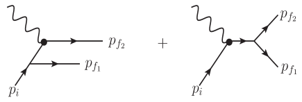
Figure 7: Single-radiation graphs contributing to scalar scattering from an external current, at first order in the coupling $\lambda$, denoted by ${\cal A}_{\,S}$ in the text.

In our chosen configuration, the first term of Eq. (1.66) is collinearly enhanced, but one easily verifies that the collinear enhancement is precisely cancelled at leading power in $\beta$ by the contribution of Eq. (1.65): at this order, we have indeed built a non-singular version of the scattering matrix in the collinear limit. Ref. [30] showed that this cancellation persist to all order in perturbation theory for soft enhancements in QED, while Ref. [59] proved it in general for a non-abelian theory. A few observations are in order.

• Perhaps most remarkably, in the coherent state picture the cancellation of singularities does not involve combining real and virtual corrections to scattering amplitudes. Indeed, as illustrated in the simple example above, matrix elements for real radiation and virtual corrections to the Born process are treated separately: for the first, the coherent state contribution subtracts the leading-power enhancement, that would lead to divergences upon phase-space integration; for the second, the leading-power enhancement is subtracted at the level of the loop integrand, so that loop integrals becomes finite.

• It is clear from the procedure leading to Eq. (1.60) that there is ample freedom in choosing what to include in the ‘asymptotic’ behaviour of the Hamiltonian, and therefore in the coherent state operator: depending on the application one has in mind, one might want to include in the asymptotic dynamics also terms that do not lead to divergences in the amplitudes, or sub-leading powers in the resolution parameter [168, 169]. This could provide an interesting avenue to explore infrared enhancements, and eventually resummations, beyond leading power, a subject that has recently received considerable attention, and could lead to relevant phenomenological applications (see, for example, [136] and references therein).

• It should also be clear from Eq. (1.60) and Eq. (1.61) that the perturbative expansion of the collinear coherent state operator at higher orders will not display any immediate simplifications: it will involve increasingly longer strings of creation and annihilation operators, and, since all particles meeting at collinear vertices carry non-vanishing momenta, the commutation properties do not lead to any obvious rearrangement at high orders. This is to be contrasted with the soft case in QED massive fermions, to be discussed briefly below, in Section 1.3.2. The point is perhaps best made by noting that the states generated by acting with $\Omega_{A,\,\pm}^{\dagger}(\Delta)$ on the Fock states are not really ‘coherent’ in the traditional sense: the asymptotic operator is not of the form $\exp(\alpha a^{\dagger})$, with $\alpha$ a $c$-number. Rather, it has a much more intricate structure, akin to $\exp(a^{\dagger}aa+{\it h.c.})$: in the presence of collinear dynamics, one should properly talk of generalised coherent states.

1.3.2 Soft divergences in QED

When moving on to the much more interesting case of massless gauge theories, it becomes unavoidable to grapple with issues related to the superposition of soft and collinear singularities. In QED, the latter are only relevant in the presence of massless charged particles, while in the non-abelian case they are unavoidable, as gluons must be massless and are charged. In such cases, the natural thing to do is to split the asymptotic hamiltonian into soft and collinear contributions, as

$$H_{A}^{E}(t)\,=\,H_{S}^{E}(t)+H_{C}^{E}(t)\,,$$ (1.67)

assigning the soft-collinear sector either to $H_{S}^{E}$ or to $H_{C}^{E}$, and avoiding double counting. To get a feeling of how that might work, notice that the boundary of the asymptotic region is defined by imposing a ‘small’ violation of energy conservation at the interaction vertex in Eq. (1.57),

$$\left|w_{1}-w_{2}-w_{3}\right|\,<\,E\,,$$ (1.68)

where, for massless QED, we can for example take $w_{3}$ to be the photon energy. Upon enforcing momentum conservation in the massless case, this becomes

$$\left|w_{1}-w_{3}-\sqrt{w_{1}^{2}+w_{3}^{2}-2w_{1}w_{3}\cos\theta_{13}}\,\right|\,<\,E$$ (1.69)

where $\theta_{13}$ is the angle between the momentum ${\bf k}_{3}$ of the photon and the momentum ${\bf k}_{1}$ of the charged particle. Considering for example the case in which the photon is emitted by an incoming ‘electron’, the physically relevant branch of the inequality in Eq. (1.69) establishes that the boundary of the asymptotic region is a hyperbola in the $w_{3}$-$\cos\theta_{13}$ plane, so that Eq. (1.69) becomes

$$\cos\theta_{13}\,>\,\left(1+\frac{E}{w_{1}}\right)-\frac{E}{w_{3}}\left(1+\frac{E}{2w_{1}}\right)\,,$$ (1.70)

depicted in Fig. 8. Clearly, the precise shape of the boundary between the asymptotic region and the hard-scattering region is not relevant, and one could just as well introduce separate cutoffs in energy and angle, as also suggested in Fig. 8: what matters is that the soft and collinear regions overlap. As a consequence, $H_{S}^{E}$ and $H_{C}^{E}$ in Eq. (1.67) do not commute, and the coherent state operator can only be factorised into soft and collinear contributions up to commutator terms [57].

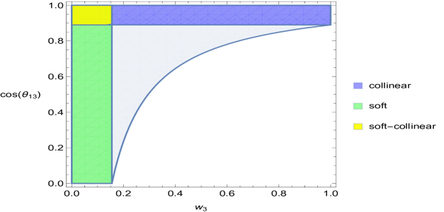
Figure 8: Asymptotic and hard regions for a massless gauge theory, with a soft-collinear overlap.

In the case of QED with massive fermions, one need not consider the collinear region at all; furthermore, one may exploit the fact that the soft part of the asymptotic hamiltonian is considerably simpler than its collinear counterpart, since, at leading power in the soft momentum, one may neglect the recoil of the hard emitting fermion. A straightforward analysis for massive QED [30] leads to the expression

$$H_{S}^{E}(t)\,=\,\int\widetilde{dk}\,\widetilde{dp}\,\frac{e}{w_{p}}\,\theta\left(E-{\bf p}\cdot{\bf k}\right){\cal H}_{\rm eik}({\bf p},{\bf k};t)\,,$$ (1.71)

where ${\bf p}$ is the momentum of the emitting fermion, ${\bf k}$ is the photon momentum, and we have introduced the (eikonal) momentum-space Hamiltonian density

$${\cal H}_{\rm eik}({\bf p},{\bf k};t)\,=\,\rho({\bf p})\,\sum_{\lambda}{\bf p}\cdot{\bf\epsilon}_{\lambda}({\bf k})\,\Big{[}a_{\lambda}({\bf k}){\rm e}^{-{\rm i}\,\widehat{{\bf p}}\cdot{\bf k}\,t}+{\it h.c.}\Big{]}\,,$$ (1.72)

where $\lambda$ is the photon polarisation and $\epsilon_{\lambda}$ the corresponding polarisation vector. Crucially, we have been able to neglect ${\bf k}$ in all factors that are regular as $w_{k}\to 0$: creation and annihilation operators for the fermions are then evaluated at the same momentum ${\bf p}$, and they organise themselves to construct the fermion number operator

$$\rho({\bf p})\,=\,\sum_{s}\Big{[}b_{s}^{\dagger}({\bf p})b_{s}({\bf p})-d_{s}^{\dagger}({\bf p})d_{s}({\bf p})\Big{]}\,.$$ (1.73)

This simplification is at the heart of all subsequent developments in QED: it means, in particular, that for ordinary Fock states involving a fixed finite number of charged particles, which are eigenstates of $\rho({\bf p})$, the coherent state operator takes the standard form $\exp(\alpha a^{\dagger})$, with $\alpha$ a $c$-number. The well-known properties of ordinary coherent states can then be exploited to perform an all-order analysis. It is important to notice that the crucial simplification leading to Eq. (1.72) is spin-independent: minimal coupling of the photon to a conserved matter current always leads, in the soft limit, to a Hamiltonian expressed in the terms of the appropriate number operator. The spin-independence of the soft approximation will play an important role in many of the developments discussed in the coming sections.

It is clear that the coherent state approach provides in principle a conceptually satisfactory solution to the infrared problem, directly emerging from correcting the inadequate approximation of asymptotic dynamics that is at the root of soft and collinear divergences of ordinary $S$ matrix elements. Over the years, a number of authors have contributed to elucidating the interpretation of the method, providing precise definitions of the finite matrix elements that emerge, and working towards practical applications [170, 171, 172, 173, 174, 175, 176, 177, 178, 179]. As we will see, however, phenomenological work in QCD has mostly followed a different approach, which we will sketch in Section 1.4 and develop in the rest of our review. On the other hand, quite interestingly, the recent symmetry-based interpretation of infrared limits on the ‘celestial sphere’ [161] can be linked to coherent states [180]. This has lead to a number of new studies and applications [158, 181, 182, 183, 184, 185], including the case of gravity [186, 187, 188, 189], and it is to be expected that further developments will be forthcoming.

1.4 What to do in QCD

In the previous sections we have sketched three partial solutions to the infrared problem: an explicit all-order calculation in the abelian case, displaying exponentiation and cancellation of singular contributions, in Section 1.1; a general proof of the cancellation of singularities in any theory with massless particles, in Section 1.2; and the outline of the construction of an improved Hilbert space, where the $S$-matrix becomes well defined, in Section 1.3. Unfortunately, none of these arguments is fully adequate to tackle the practical problems that arise in the most relevant physical application, QCD at colliders; furthermore, many beautiful and interesting structural and theoretical aspects of the problem remain hidden.

To be more specific, the QED ‘solution’ does not generalise to the non-abelian theory because the presence of massless interacting gluons inevitably brings collinear divergences into the game, even if one couples only massive matter fields to the Yang-Mills theory. This, in turn, makes it necessary to consider initial-state degeneracies in the KLN sum. Next, of course, come the problems related to confinement, and the non-perturbative aspects of the non-abelian theory. In QED, the true asymptotic states are not Fock states, but they are not drastically different either, since at least they can be expressed in terms of the same degrees of freedom, and we expect that a perturbative construction of asymptotic coherent states, starting from Fock states, will remain close to the true result. In QCD, the true asymptotic states are hadrons, and they are not perturbatively related to Fock states built out of quarks and gluons. This makes it essentially unfeasible to resort to the KLN theorem to compute physical QCD cross sections: we would need to include in our calculations multi-parton states, but in practice we do not know how such multi-parton states contribute to the wave functions of the hadrons we are colliding. Similarly, a perturbative construction of QCD coherent states will mix Fock states with different parton content, with specific weights and phases dictated by the perturbative asymptotic hamiltonian: these weights and phases are bound to be drastically altered by non-perturbative effects, in ways that are not under control.

With limited help from the general cancellation theorems that we have outlined, perturbative QCD relies upon the pillar of asymptotic freedom, and a mix of rigourous all-order perturbative analyses with physical understanding strongly supported by experiment. There are basically two categories of hadronic observables that are accessible by means of perturbative tools, and we briefly outline them below.

1.4.1 Infrared-safe cross sections

In a situation without strongly-interacting particles in the initial state (in other words, at lepton colliders) one can hope to mimic the ‘QED solution’, looking for observables that are sufficiently inclusive in the soft and collinear radiation, in order for the associated divergences to cancel. The first step is then to introduce soft and collinear regulators, in order to construct a perturbative estimate of the chosen observable. In the renormalised theory, quark masses $m_{i}(\mu)$, running with the renormalisation scale $\mu$, would act as a partial collinear regulator, and a gluon mass $m_{g}$ would regulate all infrared divergences, were it not for the technical difficulties associated with the breaking of gauge invariance. In practice, the only workable and universally applied infrared regularisation scheme for non-abelian theories is dimensional regularisation, where, after renormalisation, one takes $d=4-2\epsilon$, with $\epsilon<0$. One then proceeds to compute a parton-level prediction for the observable, which we take to depend upon a set of momenta $\{p_{i}\}$. We write it as

$$\sigma_{\rm part}\,=\,\sigma_{0}\,{\cal F}_{\rm part}\left(\frac{p_{i}\cdot p_{j}}{\mu^{2}},\alpha_{s}(\mu);\frac{m}{\mu},\epsilon\right)\,,$$ (1.74)

where $m$ is a parton-level mass scale, used as an infrared regulator. If the observable is sufficiently inclusive, in other words sufficiently insensitive to soft and collinear radiation, the perturbative parton-level prediction will have a finite limit when the infrared regulator(s) are removed. One can then write [61]

$$\sigma_{\rm part}\,=\,\sigma_{0}\,{\cal F}_{\rm part}\left(\frac{p_{i}\cdot p_{j}}{\mu^{2}},\alpha_{s}(\mu);0,0\right)\,+\,{\cal O}\left[\left(\frac{m}{\mu}\right)^{\!p},\epsilon\right]\,,$$ (1.75)

with $p$ a positive integer. Observables with this property are called infrared safe, and general criteria are available to ascertain the existence of the finite limit in Eq. (1.75) (some examples will be given in Section 2.6), which can be established to all orders in perturbation theory. At this point, two further steps are needed in order to treat the leading term of Eq. (1.75) as a reliable estimate of the corresponding hadronic observable. First, we need to be able to trust the perturbative expansion, at least as an asymptotic expansion. This happens in QCD if it is appropriate to choose the renormalisation scale $\mu$ as a hard scale, $\mu\gg\Lambda_{\rm QCD}$, which is the case if all Mandelstam invariants $p_{i}\cdot p_{j}$ in Eq. (1.75) are large in the same sense. The second step is more subtle, and ultimately involves a degree of assumption: we interpret the weak dependence of $\sigma_{\rm part}$ on the infrared regulators as indicating a weak dependence on long-time, long-distance physical processes, happening at length scales $\Delta x\gg\hbar/\Lambda_{\rm QCD}$. These are the length scales at which partons hadronise and color is neutralised. We conclude that our parton-level perturbative estimate of the observable will only be weakly affected by hadronisation corrections, which will be expected to be of parametric size $\left(\Lambda_{\rm QCD}/\mu\right)^{q}$, with $q$ a positive integer. In many well-motivated models of power corrections, where $m$ in Eq. (1.74) is related to a gluon mass (see for example [200, 201]), one finds that $q=p$, which is generally supported by arguments based on the OPE (when available), and consistent with experimental data.

It is worth pointing out that this last step, translating from parton to hadron language, relies on a picture of confinement which is very strongly supported by an immense body of experimental data, but cannot be proved within QCD until better non-pertubative techniques become available. One could, in principle, imagine a world in which, as partons ‘cool’, flowing away from the hard scattering, they meet a sharp confining transition which drastically redistributes their momenta. The data show instead that confinement and hadronisation after a hard collision happen locally in momentum space, so that the parton configuration emerging from the hard scattering is closely mirrored by the hadron distribution detected at large distances, with corrections that are parametrically negligible at high energies – a picture that was described as ‘Local Parton-Hadron Duality’ in the early decades of QCD [202, 203].

1.4.2 Factorisable cross sections

Whenever strongly interacting particles are present in the initial state, the relatively simple picture of infrared safety discussed in Section 1.4.1 is bound to break down. As discussed in a simple example in Section 2.8, processes initiated by massless partons are affected by collinear enhancements, which can be associated with the radiation of energetic gluons form the initiating parton. Such radiation changes the kinematics of the subsequent hard scattering, and therefore the singularity cannot possibly be cancelled by virtual corrections to the Born process with the given initial state: the KLN cancellation will require the inclusion of degenerate initial configurations.

Since, as discussed above, implementing the initial-state KLN sum is, to say the least, impractical, we would reach an impasse. Fortunately, for high-energy scattering, a new ingredient comes to the rescue: the separation of scales between the hard scattering and hadronisation. Intuitively, we understand that the collinear divergence associated with radiation from the initial state is due to the fact that emission at very early times is not sufficiently suppressed, since the particles involved remain close to the mass shell after the splitting. On the other hand, one would like to argue that such early emissions should properly be associated with the wave function of the initial state, rather than with the hard scattering. In general, this intuitive, semi-classical picture breaks down when quantum corrections are included, since all sub-processes contributing to the cross section interfere. If, however, hadrons are formed on space-time scales that are widely separated from the short-distance hard-scattering process, one may expect the quantum-mechanical interference to be suppressed. Proving that this is indeed the case in a relativistic quantum field theory requires an intricate diagrammatic analysis, which in some cases can be short-circuited with powerful effective field theory arguments. We will introduce, at amplitude level, some of the techniques entering factorisation proofs in Section 3. At the level of observable cross sections, the relevant arguments are summarised in excellent existing reviews, such as Refs. [60, 61, 96]. In this Introduction, we simply present very briefly the result of these arguments.

Since the requirements of infrared safety discussed in Section 1.4.1 are unchanged, we consider again a sufficiently inclusive cross section $\sigma_{\rm part}$ for a partonic process, this time involving identified partons in the initial, and possibly the final state. We assume that the Mandelstam invariants $p_{i}\cdot p_{j}$ of the partonic process are all much larger that the hadronic scale $\Lambda_{\rm QCD}^{2}$. We then introduce at parton level a mass parameter $m$, acting as an infrared cutoff, and a factorisation scale $\mu_{f}$, separating the energies characteristic of the hard scattering, $\mu^{2}\sim p_{i}\cdot p_{j}$ from the hadronic scale. One then finds that the partonic cross section can be factorised, in general in the form of a convolution, which we write, somewhat formally, as

$$\sigma_{\rm part}\,=\,{\cal S}_{\rm long}\left(\frac{m^{2}}{\mu_{f}^{2}}\right)\star{\cal H}_{\rm short}\left(\frac{p_{i}\cdot p_{j}}{\mu^{2}},\frac{\mu_{f}^{2}}{\mu^{2}}\right)\,+\,{\cal O}\left[\left(\frac{m^{2}}{\mu_{f}^{2}}\right)^{\!p}\,\right]\,,$$ (1.76)

where $\star$ denotes the appropriate convolution and, again, $p$ is a positive integer. Up to power-suppressed corrections, Eq. (1.76) separates the long-distance dynamics, governed by the factor ${\cal S}_{\rm long}$, which contains all the singular dependence on the cutoff $m$, from the short-distance hard scattering factor ${\cal H}_{\rm short}$, which is free of infrared singularities. Intuitively, ${\cal S}_{\rm long}$ collects contributions from (soft and) collinear radiation at early and late times, which build up probability distributions for initial and final states of the hard scattering: such contributions are expected to be universal, i.e. independent of the particular hard process being considered; on the other hand, they are not calculable in perturbative QCD, and must be extracted from experiments. On the contrary, ${\cal H}_{\rm short}$ collects contributions from short-distance, off-shell exchanges: these are infrared finite, and thus we expect them to be reliably calculable in perturbation theory; on the other hand, they are clearly process-dependent.

The factorisation of un-cancelled infrared singularities described by Eq. (1.76), and based on separation of scales, has evident analogies with the handling of ultraviolet singularities by means of renormalisation: also in this case, singular contributions have been assigned to universal factors, which must be determined experimentally, and finite contributions from processes happening at laboratory scales have become calculable; we will pursue this analogy a little further in Section 4. As was the case for infrared safe observables, also for factorisable cross sections the application of Eq. (1.76) to hadronic cross sections relies to some extent on the assumption, well supported by experiments, that non-perturbative effects do not drastically disrupt the dynamical pattern emerging at parton level: we interpret Eq. (1.76) as stating that long-distance dynamics is factorisable for inclusive cross sections, up to power-suppressed contributions; we then substitute the divergent contributions to ${\cal S}_{\rm long}$ with the appropriate finite, experimentally measured, combinations of parton distributions and fragmentation functions; we expect the result to be accurate up to corrections suppressed by $(\Lambda_{\rm QCD}/\mu)^{q}$, with strong arguments suggesting that $q=p$ in many cases. We recall that Eq. (1.76) follows from the OPE for highly inclusive cross sections such as DIS structure functions, and it was proved to all orders in perturbation theory for parton annihilation into colour-singlet final states in Refs. [204, 205]. A crucial argument to extend this all-order proof to inclusive jet cross sections was given in Ref. [206], while for general collider observables the debate on the boundaries of applicability of expression of the form of Eq. (1.76) continues (see, for example, Ref. [207] and the extensive discussions in [67]).

2 Finite orders: tools and results

After discussing the (pre-)history of the infrared problem in our Introduction, we now turn to the ‘modern’ viewpoint, which is predominantly driven by the practical requirements of large-scale perturbative calculations for applications at high-energy colliders. This means that the focus is the non-abelian theory, and it largely implies that the infrared regulation scheme is dimensional regularisation. In the present section, we will briefly present the treatment of soft and collinear singularities in simple one-loop QCD calculations. This is of course well-known textbook material, and we will only sketch the relevant calculations: this simple context will, however, allow us to introduce some of the tools of the trade, that we will employ in a more abstract context in later Sections of this review. Following the arguments in Section 1.4, we will first present the case of infrared-safe cross sections at lepton colliders, introducing concepts relevant to Section 4, and then we will sketch the derivation of collinear factorisation in one-loop Deep Inelastic Scattering, which will prepare some grounds for the discussion in Section 6.

2.1 Infrared safety: the total cross section

The prototype infrared-safe observable at lepton colliders is the total cross section for lepton annihilation into hadrons. By definition, it is expected to be insensitive to the radiation of soft and collinear massless particles, and the parton-level result bears the simplest possible relation to the hadronic observable, since all radiated partons must turn into hadrons with unit probability. These expectations are borne out by the explicit calculation in dimensional regularisation, which we now outline: the Bloch-Nordsieck-like cancellation of soft and collinear poles between real and virtual contributions will be on display.

Working in the perturbative regime, with a center-of-mass squared energy $s$ much larger than hadron masses, we consider the process in which a massless lepton of momentum $k_{1}$ annihilates with an anti-lepton of momentum $k_{2}$, with $k_{1}^{\mu}+k_{2}^{\mu}=q^{\mu}$, and $q^{2}=s$. The annihilation of the two leptons produces a photon which later decays into massless partons. Since we will remain at leading order in QED, but will later consider all orders in the strong coupling, it is worthwhile to give general expressions for the ingredients entering the cross section. We start from the definition

$$\sigma_{\rm tot}\left(q^{2}\right)\,=\,\frac{1}{2q^{2}}\,\sum_{X}\int d\Phi_{X}\,\frac{1}{4}\sum_{\rm spin}\Big{|}{\cal A}\big{(}k_{1}+k_{2}\rightarrow X\big{)}\Big{|}^{2}\,,$$ (2.1)

where $X$ is a generic strongly-interacting final state, $\Phi_{X}$ is the corresponding phase space measure, and $2q^{2}$ is the flux factor for massless particles. At leading order in QED, one can split the calculation into leptonic and hadronic tensors, according to

$$\sigma_{\rm tot}\left(q^{2}\right)\,\equiv\,\frac{1}{2q^{2}}\,L_{\mu\nu}(k_{1},k_{2})\,H^{\mu\nu}(q)\,,$$ (2.2)

where the leading-order leptonic tensor, including the photon propagator, is

$$L^{\mu\nu}(k_{1},k_{2})\,=\,\frac{e^{2}}{q^{4}}\,\Big{(}k_{1}^{\mu}k_{2}^{\nu}+k_{1}^{\nu}k_{2}^{\mu}-k_{1}\cdot k_{2}\,g^{\mu\nu}\Big{)}\,.$$ (2.3)

The hadronic tensor, on the other hand, can be expressed (in principle non-perturbatively in the strong interactions) in terms of matrix elements of the electromagnetic current, as

$$H_{\mu\nu}(q) = e^{2}Q_{f}^{2}\,\sum_{X}\left\langle\smash{0}{\vphantom{1}}\right|J_{\mu}(0)\left|\smash{X}{\vphantom{1}}\right\rangle\,\left\langle\smash{X}{\vphantom{1}}\right|J_{\nu}(0)\left|\smash{0}{\vphantom{1}}\right\rangle\,(2\pi)^{4}\delta^{4}\left(q-p_{X}\right)$$ (2.4)

$$\equiv \big{(}q_{\mu}q_{\nu}-q^{2}g_{\mu\nu}\big{)}\,H(q^{2})\,.$$

At parton level, the current $J_{\mu}(x)$ in (single-flavour) QCD is simply the conserved Dirac current $J_{\mu}(x)=\overline{\psi}(x)\gamma_{\mu}\psi(x)$, and the simplest state contributing to the sum is a two-particle state containing a quark-antiquark pair. In the second line of Eq. (2.4) we have used current conservation to extract the transverse tensor structure, expressing the result in terms of the single scalar function $H(q^{2})=H^{\mu}_{\,\,\,\mu}(q)/((d-1)q^{2})$. Using now the fact that the leptonic tensor is also transverse, we express the total cross section in terms of the trace of the hadronic tensor as

$$\sigma_{\rm tot}\left(q^{2}\right)\,\equiv\,\frac{e^{2}}{2q^{4}}\,\frac{1}{3}\big{(}-g_{\mu\nu}\,H^{\mu\nu}(q)\big{)}\,.$$ (2.5)

The calculation of the trace of the hadronic tensor up to ${\cal O}(\alpha_{s})$ is a classic result (see for example [2]), and, in the meantime, the perturbative calculation has been pushed to an extraordinary ${\cal O}(\alpha_{s}^{4})$ accuracy [208, 209, 210, 211]. To summarise the ${\cal O}(\alpha_{s})$ calculation, we introduce the first tool in our toolbox.

2.2 A tool: cut diagrams

Unitarity tells us that the imaginary part of a Feynman diagram $G$ for a scattering amplitude is given by the sum of all cut diagrams that can be constructed from it. A cut diagram is built by partitioning the original graph into two subgraphs, one containing initial state particles, while the second one contains the final state; propagators that are thus ‘cut’ must be replaced with the mass-shell condition. This foundational result suggests that it should be possible to construct a set of Feynman rules to compute directly squared amplitudes, and thus cross sections: it is easy to convince oneself that this is indeed the case. The crucial identity is displayed in Fig. 9, where the continuous line can be taken to represent any charged particle - for definiteness, we consider a quark radiating a set of gluons. In words, a charged line in a Feynman diagram can be complex-conjugated by reversing the charge flow, with the understanding that the signs of explicit factors of $i$ must also be changed. This allows, for fixed final-state momenta, to ‘join’ the end of the line in the original diagram with the beginning of the complex-conjugate line.

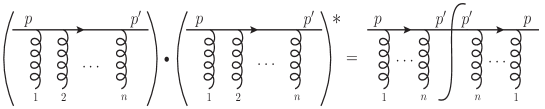
Figure 9: Expressing the squared modulus of fermion line contribution to a Feynman diagram in terms of a cut diagram.

In the case of a quark radiating gluons, the identity in Fig. 9 follows from the Clifford algebra identity

$$\Big{[}\overline{u}_{s^{\prime}}(p^{\prime})\,\gamma_{\mu_{n}}\,\ldots\,\gamma_{\mu_{1}}\,u_{s}(p)\Big{]}^{*}\,=\,\overline{u}_{s}(p)\,\gamma_{\mu_{1}}\,\ldots\,\gamma_{\mu_{n}}\,u_{s^{\prime}}(p^{\prime})\,,$$ (2.6)

with similar identities holding for other combinations of particle and anti-particle spinors. Colour indices also obey the line-reversal rule, thanks to the hermiticity of the generators of the Lie algebra

$$\Big{[}T^{a}_{\phantom{a}ij}\Big{]}^{*}\,=\,T^{a}_{\phantom{a}ji}\,.$$ (2.7)

Identities like Eq. (2.6) or Eq. (2.7) are, of course, not accidents of the Clifford algebra, or of a specific symmetry group: they follow from the hermiticity of the Hamiltonian, which in turn underpins the unitarity of the theory.

One can now go on and observe that the cut in Fig. 9 can be interpreted as imposing the mass shell condition (accompanied by the constraint establishing the positivity of the energy of the outgoing particle). If one further performs the sum over final-state spins, the cut-line Feynman rule corresponds to replacing a would-be propagator with momentum $p$ with its imaginary part, accompanied by the propagator numerator arising from the spin sum:

$${\rm i}\frac{p\hskip-4.49997pt/+m}{p^{2}-m^{2}+{\rm i}\eta}\,\to\,(2\pi)\,\delta(p^{2}-m^{2})\,\theta(p_{0})\sum_{s}u_{s}(p)\overline{u}_{s}(p)\,\equiv\,(2\pi)\delta_{+}(p^{2}-m^{2})\left(p\hskip-4.49997pt/+m\right)\,.$$ (2.8)

Finally, one may wish to integrate final-state momenta over some range, in order to build an observable cross section. One notes then that, upon interfering a diagram with $k$ loops and $p$ final-state particles with another diagram with $k^{\prime}$ loops, and of course the same final particles, the graph constructed according to the rules just described will have $k+k^{\prime}+p-1$ loops, including $p-1$ cut loops. Integrating over the $p-1$ loop momenta, with $p$ mass-shell conditions from the cut propagators, builds up the phase space integration appropriate for an inclusive cross section: one can then, eventually, insert in that phase space a weight function identifying the desired observable. In a sense, the procedure just outlined reverses the standard proofs of unitarity for Feynman graphs: we start out with an attempt to build Feynman rules for squared matrix elements, and we end up with cut graphs. The underlying unitarity justifies the most delicate aspects of the procedure: indeed, it is far from obvious that symmetry factors and signs associated with fermion loops will match between cut and uncut graphs, but it can be shown in full generality that they do [2].

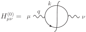
Figure 10: The tree-level hadronic tensor as a cut diagram.

In order to illustrate how this works in practice, we sketch the computation of the trace of the hadronic tensor, Eq. (2.4), at lowest order in perturbation theory; in Section 2.3 and in Section 2.4 we will outline the corresponding one-loop calculation. Looking at the cut Feynman diagram in Fig. 10, and noting that our observable is fully inclusive, we readily find

$$H_{\mu\nu}^{(0)}(q)\,=\,-e^{2}Q_{f}^{2}\int\frac{d^{4}k}{(2\pi)^{4}}(2\pi)\delta_{+}(k^{2})(2\pi)\delta_{+}\left((k-q)^{2}\right){\rm Tr}\left[k\hskip-4.49997pt/\gamma_{\mu}\left(k\hskip-4.49997pt/-q\hskip-4.49997pt/\right)\gamma_{\nu}\right]\,,$$ (2.9)

where $Q_{f}$ is the electric charge of quarks of flavour $f$ in units of the electron charge. Crucially, we included in Eq. (2.9) a negative sign for the fermion cut loop: failure to do so would lead to a negative total cross section. The calculation of Eq. (2.9) is now immediate: the mass-shell $\delta$ function for momentum $k$ turns the loop integral into a Lorentz-invariant phase-space integral; the second mass-shell $\delta$ function then sets $k\cdot q=q^{2}/2$; dimensional analysis dictates that the result must be proportional to $q^{2}$; the trivial angular integration determines the overall constant. Inserting the result in Eq. (2.5), and summing over colours and active flavours, one finds of course the classic value of the leading-order $R$ ratio

$$R\left(\frac{q^{2}}{\mu^{2}},\alpha_{s}(\mu^{2})\right) \equiv \frac{\sigma_{\rm tot}(e^{+}e^{-}\to{\rm hadrons})}{\sigma_{\rm tot}(e^{+}e^{-}\to\mu^{+}\mu^{-})}\,=\,R_{0}\,\sum_{n=0}^{\infty}\bigg{(}\frac{\alpha_{s}(\mu^{2})}{\pi}\bigg{)}^{\!n}\Delta_{n}\left(\frac{q^{2}}{\mu^{2}}\right)\,,$$

$$R_{0} = N_{c}\sum_{f}Q_{f}^{2}\,,\qquad\Delta_{0}\,=\,1\,.$$ (2.10)

As we will see in the next section, cut diagrams organise higher-orders calculations in a natural way, and in particular they nicely highlight the mechanism for the cancellation of infrared singularity in the spirit of the KLN theorem.

2.3 Real radiation at one loop

Following the reasoning presented in Section 2.2, the calculation of the hadronic tensor at higher orders is naturally organised by writing down the diagrams contributing to the photon-induced vacuum polarisation, and then summing over the possible positions for the cut, as illustrated at one loop in Fig. 11.

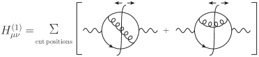
Figure 11: The one-loop hadronic tensor as a sum of cut diagrams.

It is important to note that the organisation of the calculation of a cross section in terms of cut diagrams is particularly well adapted to study the cancellation of infrared singularities. The three-particle cut shown in Fig. 11 corresponds to a contribution from real gluon radiation, integrated over phase space; when the cut is moved across a gluon emission vertex, one finds a virtual one-loop contribution, interfered with the Born process. The cancellation of infrared singularities happens, for every uncut diagram, in the sum over cut positions. This bears an intuitive relation with the mechanism for cancellation highlighted by the KLN theorem: when the radiated gluon becomes soft or collinear, and thus unresolved, the real-radiation contribution becomes physically indistinguishable from the virtual correction, and the rules of quantum mechanics require that the two configurations be summed. The KLN sum over degenerate states is thus precisely implemented by the sum over cut positions.

It is clearly desirable to have a systematic and practical method to perform the sum over cut positions at the integrand level, in order to cancel the contributions of singular configurations without having to introduce external regulators for virtual poles and phase-space integrals. This would in principle allow for a fully numerical evaluation of infrared-safe distributions in the renormalised theory. Indeed, a method along these lines was proposed in Refs. [212, 213], starting from the so-called Feynman Tree Theorem [214] (see also [215]), and is steadily being developed [216, 217, 218, 219, 220, 221, 222, 82, 223]. For the sake of our current simple example, we will follow the standard approach of treating separately the real radiation contribution, integrated over phase space, and the virtual correction: singularities in both cases will be regulated by dimensional regularisation, taking $d=4-2\epsilon$, with $\epsilon<0$, and they will, as expected, cancel in the sum.

Let us begin by writing down the general form of the three-particle cut contribution to the hadronic tensor. It reads

$$H_{\mu\nu}^{(1,R)}(q)\,\equiv\,\int\frac{d^{d}k\,d^{d}p}{(2\pi)^{2d-3}}\,\delta_{+}(k^{2})\,\delta_{+}(p^{2})\,\delta_{+}\left((q-p-k)^{2}\right){\cal H}^{(1)}_{\mu\nu}(p,k)\,,$$ (2.11)

where we take $k$ to be the gluon momentum, $p$ to be (say) the quark momentum, while ${\cal H}^{(1)}_{\mu\nu}$ is the actual squared matrix element for $\gamma^{*}\to q\bar{q}g$, computed from the sum of the three-particle cuts of the diagrams in Fig. 11; furthermore, as announced, we have promoted the loop integrations to $d$ dimensions.

It is perhaps worthwhile discussing briefly here the application of dimensional regularisation to the infrared problem. In the case of Eq. (2.11), there are no UV divergences, so one can directly take $\epsilon<0$. It is fairly obvious that this choice will properly regulate soft divergences, which arise from the uniform scaling limit $k^{\mu}\to\lambda k^{\mu}$, $\lambda\to 0$. Indeed, the $d$-dimensional measure of integration in Eq. (2.11) behaves as

$$d^{d}k\,\delta(k^{2}) \rightarrow \frac{d^{d-1}k}{k}\,\rightarrow\,dk\,k^{1-2\epsilon}\,d\Omega_{d-2}\,,$$ (2.12)

with $k=|{\bf k}|$, and $\Omega_{d-2}$ the solid angle in $d-1$ space dimensions: a negative value of $\epsilon$ clearly improves the behavior of the integrand as $k^{\mu}\to 0$. It is less obvious that taking $d>4$ will help with collinear divergences: radiated collinear particles can indeed be very energetic, and only after developing appropriate power counting tools (as we do here in Section 3) one can be sure that the method will work. In the present case, it is sufficient to write down the angular measure of integration in $d$ space-time dimensions, thus depending on $d-3$ ‘co-latitudes’ $0\leq\theta_{i}\leq\pi$, $i=1,\ldots,d-3$, and one azimuthal angle $0\leq\phi<2\pi$. The result is well known and, after simple manipulations, it can be written as

$$d\Omega_{d-2} = d\cos\theta_{d-3}\left(1-\cos^{2}\theta_{d-3}\right)^{-\epsilon}\times\ldots\times d\theta_{1}\sin\theta_{1}\,d\phi\,,$$ (2.13)

which indeed displays a suppression of potential singularities as $\theta_{d-3}\to 0$ or as $\theta_{d-3}\to\pi$, for $\epsilon<0$. Turning now again to Eq. (2.11), it is easy to convince oneself that the integrand in $d=4$ depends non-trivially on just one angle, which can be taken to be the angle between the quark and gluon three-momenta. We can then set $\theta_{d-3}=\theta_{pk}$, and integrate over the remaining angles. Choosing as integration variables

$$z\,\equiv\,\frac{2k}{\sqrt{q^{2}}}\,,\qquad\quad y\,\equiv\frac{1-\cos\theta_{pk}}{2}\,,$$ (2.14)

so that $0\leq\{z,y\}\leq 1$, and using again dimensional analysis, we can rewrite Eq. (2.11), up to an overall constant, as

$$H_{\mu\nu}^{(1,R)}(q)\,\propto\,\left(q^{2}\right)^{1-2\epsilon}\int_{0}^{1}dz\,z^{1-2\epsilon}\int_{0}^{1}dy\big{[}y(1-y)\big{]}^{-\epsilon}{\cal H}^{(1)}_{\mu\nu}(p,k)\,.$$ (2.15)

We need now to study the behaviour of the squared matrix element ${\cal H}^{(1)}_{\mu\nu}(p,k)$ in the potentially singular limits, $z\to 0$ and $y\to 0,1$. This will be done in a systematic way in Section 3, but, at this order, it is easy to extract the relevant information from the diagrams in Fig. 11: when the radiated gluon becomes soft, both the matrix element and its complex conjugate provide a factor of $1/z$; furthermore, when the gluon becomes collinear to the (massless) quark, the quark propagator provides a factor of $1/y$; when the emission is collinear to the antiquark, by momentum conservation the antiquark propagator must provide a factor of $1/(1-y)$. Altogether, the leading singularity of the squared matrix element is given by

$${\cal H}^{(1)}_{\mu\nu}(p,k)\sim\frac{1}{z^{2}\,y\,(1-y)}\,.$$ (2.16)

Noting that the $y$-dependent denominator can be partial-fractioned, we interpret this as the superposition of a soft singularity with the sum of two non-overlapping collinear singularities. Therefore both the $z$ and the $y$ integrations will yield infrared poles. A complete calculation [2] gives the result

$$\left(H^{\mu}_{\,\,\mu}\right)^{(1,R)}(q)\,\propto\,\frac{\alpha_{s}(\mu)}{\pi}\,C_{F}\,q^{2}\left(\frac{4\pi\mu^{2}}{q^{2}}\right)^{\epsilon}\left[\frac{2}{\epsilon^{2}}+\frac{3}{\epsilon}-\pi^{2}+\ldots\right]\,,$$ (2.17)

where we performed the colour sums and introduced the renormalisation scale $\mu$. The result exhibits the typical double pole in $\epsilon$, representing the superimposed soft and collinear singularities, and leading to double logarithms of $q^{2}$ in the finite terms. The single pole in $\epsilon$ could in principle arise from soft gluon emission at wide angles with respect to the quark and the antiquark, or from hard collinear gluon emission: in the present case, as we will see, the single pole in Eq. (2.17) has the latter origin. Finally, we included for future reference the ‘large’ transcendental constant $\pi^{2}$ (while not displaying the remaining rational numbers), arising from the expansion in powers of $\epsilon$ of the $\Gamma$ functions originating from the phase space integration. Such constants can play an important numerical role, amplifying the impact of radiative corrections, and in some cases they can be organised to all orders in perturbation theory, as first noted in Ref. [225]: we will return to their connection to infrared poles in later sections of our review.

2.4 Virtual corrections: the quark form factor

According to the general theorems derived in Section 1, the infrared poles in Eq. (2.17) must cancel against the contributions of two-particle cuts to the diagrams in Fig. 11. To any order in perturbation theory, such cut diagrams build up the interference between the Born amplitude for $\gamma^{*}\to q\bar{q}$ and the quark form factor, which is defined by

$$\Gamma_{\mu}\!\left(p_{1},p_{2};\mu^{2},\epsilon\right)\,\equiv\,\left\langle\smash{p_{1},p_{2}}{\vphantom{1}}\right|J_{\mu}(0)\left|\smash{0}{\vphantom{1}}\right\rangle\,=\,\bar{u}(p_{1})\gamma_{\mu}v(p_{2})\,\Gamma\left(\frac{q^{2}}{\mu^{2}},\alpha_{s}(\mu^{2}),\epsilon\right)\,,$$ (2.18)

providing all purely virtual contributions to Eq. (2.4). The quark form factor is a fundamental object in perturbative QCD, and provides a crucial ingredient for the calculation of all cross sections involving only two hard quark jets, either in the initial or in the final state. As we will see in Section 4, it is also the simplest object for which the resummation of infrared poles to all orders can be completely carried out [62, 63, 64, 65, 226, 68]. Its explicit form in dimensional regularisation is now known to three loops [227, 228, 229], while all infrared poles are known to four loops [230, 231]. Before making a few comments on the one-loop calculation, we will point out a few general properties of the form factor, which will be crucial in Section 4. We will then also take the opportunity to develop one more tool in our toolbox, the $d$-dimensional running coupling, discussed below in Section 2.5.

First of all, notice that, in the massless case, the vector form factor $\Gamma_{\mu}$ in Eq. (2.18) is characterised by a single scalar function $\Gamma$, with the vector structure being fixed at tree-level. Next, observe that the quark form factor is defined as a matrix element of the conserved electromagnetic current. As such, it does not get renormalised: after the renormalisation of the QCD coupling there is no need for an overall multiplicative renormalisation associated with the QED vertex. This is of course a consequence of the QED Ward identity, but it has a clear physical motivation: if switching on the strong interactions were to cause a change in electric charges, it would be hard(er) to explain the precise experimental relations between the electric charges of quarks and leptons. The non-renormalisation of the form factor implies that it obeys a renormalisation group equation with a vanishing anomalous dimension. In dimensional regularisation, we write

$$\left(\mu\frac{\partial}{\partial\mu}+\beta\left(\epsilon,\alpha_{s}\right)\frac{\partial}{\partial\alpha_{s}}\right)\Gamma\left(\frac{q^{2}}{\mu^{2}},\alpha_{s}(\mu^{2}),\epsilon\right)\,=\,0\,.$$ (2.19)

The crucial point in Eq. (2.19) is that, since we are working with a divergent quantity, which is mathematically well-defined only away from $d=4$, we need to use the $d$-dimensional version of the $\beta$ function. This will have pivotal consequences for the exponentiation of infrared poles, discussed in the following.

For the moment, to complete our NLO example, we concentrate on summarising the evaluation of the form factor at one loop.

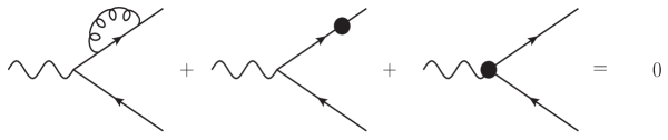
Figure 12: One-loop diagrams giving a vanishing contribution to the quark form factor, including UV counterterms.

The one-loop calculation in dimensional regularisation, in the massless case, is simplified by the fact that only the vertex-correction diagram contributes. The remaining diagrams, including ultraviolet counterterms, are displayed in Fig. 12: the fact that they give a vanishing contribution can be understood in two slightly different ways. On the one hand, we can simply note that scale-less integrals are defined to vanish in dimensional regularisation, which applies to the self-energy correction to the massless quark propagator; the fact that the sum of the two UV counterterms vanishes is then a consequence of the QED Ward identity. On the other hand, we can interpret the vanishing of the self-energy as the cancellation of a UV pole with an IR pole near $d=4$, an interpretation that can be checked by introducing auxiliary regulators; the quark field renormalisation counterterm in the MS scheme, which cancels the UV pole, must then be equal to the IR pole of the self-energy diagram; the Ward identity thus forces the UV vertex counterterm to be equal (with opposite sign) to the IR pole of the propagator correction.

The vertex correction diagram is of course a textbook exercise: here we just quickly pause to stress the power-counting properties of the terms it comprises. A straightforward application of the Feynman rules gives a decomposition into tensor integrals in the form

$$\Gamma_{\mu}^{(1)}\,=\,c_{\mu}I_{0}+c_{\mu\alpha}I_{1}^{\alpha}+c_{\mu\alpha\beta}I_{2}^{\alpha\beta}\,,$$ (2.20)

with the tensor integrals defined by

$$\Big{\{}I_{0},I_{1}^{\alpha},I_{2}^{\alpha\beta}\Big{\}}\,\equiv\,\int\frac{d^{d}k}{(2\pi)^{d}}\,\frac{\big{\{}1,k^{\alpha},k^{\alpha}k^{\beta}\big{\}}}{\left(k^{2}+{\rm i}\eta\right)\left[\left(p_{1}-k\right)^{2}+{\rm i}\eta\right]\left[\left(p_{2}+k\right)^{2}+{\rm i}\eta\right]}\,.$$ (2.21)

Naïve power counting immediately shows that only the tensor integral $I^{\alpha\beta}_{2}$ can contribute to the UV pole, while only the scalar integral $I_{0}$ can contribute to the soft pole. The vector integral $I^{\alpha}_{1}$ appears free of both IR and UV singularities, but - since the suppression provided by the numerator is direction-dependent - it still can (and does) contribute a collinear pole. Clearly, one needs a more precise definition of power counting in infrared regions, which we will address in Section 3. When the dust settles, one finds the well known result

$$\Gamma^{(1)}\,=\,-\,\frac{\alpha_{s}}{4\pi}\,C_{F}\,\left(\frac{4\pi\mu^{2}}{-q^{2}-{\rm i}\eta}\right)^{\!\!\epsilon}\,\frac{\Gamma^{2}(1-\epsilon)\Gamma(1+\epsilon)}{\Gamma(1-2\epsilon)}\,\left[\frac{2}{\epsilon^{2}}+\frac{3}{\epsilon}+\ldots\right]\,.$$ (2.22)

Once again, Eq. (2.22) exhibits the hallmarks of all calculations of IR singularities of massless gauge-theory amplitudes in dimensional regularisation: every loop carries a double pole, corresponding to the superposition of a soft singularity with the sum of (in this case) two non-overlapping collinear singularities. One then finds a single pole, which can be due to soft gluons emitted at wide angles with respect to hard momenta, or (as is the case here) to the radiation of hard collinear gluons. We also note that, as we are computing the time-like form factor ($q^{2}>0$), the amplitude has an imaginary part associated with the two-particle cut. In the presence of a double infrared pole, this imaginary part provides a further source of potentially large perturbative corrections to physical cross sections, in the form of ‘large’ transcendental constants such as $\pi^{2}$. Indeed, expanding Eq. (2.22) in powers of $\epsilon$, one must use

$$\left(-q^{2}-{\rm i}\eta\right)^{-\epsilon}\,=\,\big{(}q^{2}\big{)}^{-\epsilon}{\rm e}^{{\rm i}\pi\epsilon}\,=\,\big{(}q^{2}\big{)}^{-\epsilon}\left(1+{\rm i}\pi\epsilon-\frac{\pi^{2}}{2}\epsilon^{2}+\ldots\right)\,.$$ (2.23)

The ${\cal O}(\epsilon)$ imaginary part will cancel when computing physical observables, but the ${\cal O}(\epsilon^{2})$ contribution will combine with the double infrared pole and can give a sizeable contribution. Such large constant contributions have been studied for a long time [225], and in many relevant cases they can be organised in exponential form to all orders in perturbation theory [226, 68, 233, 234]. For the total cross section that we are computing, it turns out that at one loop all transcendental constants cancel in the sum of real and virtual corrections: interfering Eq. (2.22) with the Born matrix element, and properly combining the result with Eq. (2.17), one finally gets the well-known result

$$R\left(\frac{q^{2}}{\mu^{2}},\alpha_{s}(\mu^{2})\right)\,=\,R_{0}\,\bigg{(}1\,+\,\frac{\alpha_{s}(\mu^{2})}{\pi}+{\cal O}\big{(}\alpha_{s}^{2}\big{)}\bigg{)}\,.$$ (2.24)

The natural question at this point is to what extent one can maintain the cancellation of infrared poles, while allowing for a more detailed (or less inclusive) treatment of real radiation. Before tackling that question, we introduce a second important tool in our toolbox.

2.5 A tool: the $d$-dimensional running coupling

Using the renormalisation group to explore quantum field theories away from dimension $d=4$ is a standard tool of statistical field theory [235, 236, 237], but not as widely used in the context of perturbative QCD. It offers, however, a simple and powerful method to sum and exponentiate infrared singularities, in a way which is directly comparable to diagrammatic calculations [68]. In particular, as we will see, it provides an elegant way to bypass the Landau pole, thus leading naturally to a ‘purely pertubative’ resummation of infrared effects [69]. The starting point is the well-known relation between the bare and renormalised couplings in $d=4-2\epsilon$,

$$\alpha_{0}\,=\,\mu^{2\epsilon}\alpha_{s}(\mu)Z_{\alpha}\,,$$ (2.25)

which leads to the presence of an $\epsilon$-dependent term, linear in $\alpha_{s}$, in the $\beta$ function. We write

$$\beta\left(\epsilon,\alpha_{s}\right)\,\equiv\,\mu\frac{\partial}{\partial\mu}\,\alpha_{s}(\mu)\,=\,-2\epsilon\alpha_{s}-\frac{\alpha_{s}^{2}}{2\pi}\,\sum_{n=0}^{\infty}\,b_{n}\left(\frac{\alpha_{s}}{\pi}\right)^{n}\,,$$ (2.26)

with a normalisation chosen so that $b_{0}=(11C_{A}-2n_{f})/3$ in QCD. Notice that, in order to regularise infrared singularities, we must take $\epsilon<0$: thus, differently from what is commonly done in a statistical field theory context, we are working at $d>4$. The $\beta$ function in Eq. (2.26), therefore, is positive for sufficiently small values of $\alpha_{s}$. To get a feel for the consequences of Eq. (2.26), we may consider the one-loop approximation, setting $b_{n}=0$ for $n\geq 1$, and solve the equation for the running coupling, for fixed $\epsilon<0$, evolving the coupling from an initial scale $\mu_{0}$ to a final scale $\mu$. One easily finds the solution

$$\overline{\alpha}\left(\frac{\mu^{2}}{\mu_{0}^{2}},\alpha_{s}(\mu_{0}^{2}),\epsilon\right)\,=\,\frac{\alpha_{s}(\mu_{0}^{2})}{\left(\frac{\mu^{2}}{\mu_{0}^{2}}\right)^{\epsilon}-\frac{1}{\epsilon}\left(\!1-\left(\frac{\mu^{2}}{\mu_{0}^{2}}\right)^{\!\!\epsilon}\,\right)\frac{b_{0}}{4\pi}\,\alpha_{s}(\mu_{0}^{2})}\,,$$ (2.27)

which is non-singular (as it must be), and gives the standard result, for $\epsilon\to 0$. The most striking feature of the running coupling in Eq. (2.27) emerges already at ‘tree level’, setting also $b_{0}=0$. In order to keep the bare coupling in Eq. (2.25) independent of $\mu$, the renormalised coupling must scale as a power, so that

$$\overline{\alpha}\left(\frac{\mu^{2}}{\mu_{0}^{2}},\alpha_{s}(\mu_{0}^{2}),\epsilon\right)\,=\,\bigg{(}\frac{\mu^{2}}{\mu_{0}^{2}}\bigg{)}^{\!-\epsilon}\alpha_{s}(\mu_{0}^{2})\,,$$ (2.28)

which, in particular, means that the running coupling vanishes for $\mu\to 0$ in $d>4$

$$\overline{\alpha}\left(0,\alpha_{s}(\mu_{0}^{2}),\epsilon<0\right)\,=\,0\,.$$ (2.29)

This is not surprising, and can be understood by looking at Fig. 13: for $\epsilon<0$, the ultraviolet fixed point responsible for asymptotic freedom has moved away from the origin by a distance of order $\epsilon$; in the meantime, at the origin one finds an infrared fixed point, which forces the coupling to vanish for vanishing scale.

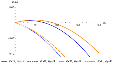
Figure 13: The $\beta$ function for different values of the regulator $\epsilon=\pm 0.1$ and the number of flavour $n_{f}$.

One may wonder what happens to the Landau pole, at one loop and beyond: this can easily be verified, by setting the denominator of Eq. (2.27) to zero and solving for the scale $\mu$, which corresponds to the common definition of the Landau pole. One finds

$$\mu^{2}\,\equiv\,\Lambda^{2}\,=\,\mu_{0}^{2}\left(1+\frac{4\pi\epsilon}{b_{0}\,\alpha_{s}(\mu_{0}^{2})}\right)^{-1/\epsilon}\,.$$ (2.30)

Once again, this reduces to usual expression for $\epsilon\to 0$; on the other hand, for negative $\epsilon$, and in particular for generic $\epsilon<-4\pi/(b_{0}\alpha_{s}(\mu_{0}^{2}))$, the Landau pole moves away from the real axis and into the complex plane. This is particularly relevant when one solves renormalisation group equations in $d>4$, as we will do in Section 4: the solutions of these equations always involve integrals of anomalous dimensions, which are functions of the running coupling, over a range of renormalisation scales. The discussion above allows to choose $\mu_{0}=0$ as the initial scale for evolution (where the coupling vanishes and the strong interactions decouple), and integrate up to our selected perturbative scale along the real axis, without encountering any singularities. It is a remarkable fact that all perturbative infrared singularities of gauge theory amplitudes, to all orders in perturbation theory, are generated by integrating finite anomalous dimensions in precisely this way, as we will see in detail in Section 4 and in Section 5. Indeed, when one expresses the running coupling evaluated at the variable scale in terms of the coupling at the fixed hard scale $\mu$, one encounters integrals of the form

$$\int_{0}^{\mu^{2}}\frac{d\lambda^{2}}{\lambda^{2}}\,\overline{\alpha}\left(\frac{\lambda^{2}}{\mu^{2}},\alpha_{s}(\mu^{2}),\epsilon\right) = \alpha_{s}(\mu^{2})\,\mu^{2\epsilon}\int_{0}^{\mu^{2}}\frac{d\lambda^{2}}{(\lambda^{2})^{1+\epsilon}}+{\cal O}(\alpha_{s}^{2})$$ (2.31)

$$= -\frac{1}{\epsilon}\,\alpha_{s}(\mu^{2})+{\cal O}(\alpha_{s}^{2})\,,$$

or, similarly,

$$\int_{0}^{\mu^{2}}\frac{d\lambda^{2}}{\lambda^{2}}\,\,\overline{\alpha}\left(\frac{\lambda^{2}}{\mu^{2}},\alpha_{s}(\mu^{2}),\epsilon\right)\,\log\bigg{(}\frac{\lambda^{2}}{\mu^{2}}\bigg{)}\,=\,-\frac{1}{\epsilon^{2}}\,\alpha_{s}(\mu^{2})+{\cal O}(\alpha_{s}^{2})\,,$$ (2.32)

and their higher-order generalisations. In the special case of gauge theories that are conformal in $d=4$, such as ${\cal N}=4$ Super-Yang-Mills theory, the $d$-dimensional running coupling obeys Eq. (2.28) exactly, and anomalous dimension integrals can give at most double infrared poles, which greatly simplifies the infrared structure of scattering amplitudes [79].

2.6 General infrared-safe observables

The calculation leading to Eq. (2.24) holds important lessons, and is amenable to broad generalisations. In fact, it would not be very informative if the only observable enjoying the cancellation of IR divergences was the total cross section, and this is indeed not what the KLN theorem states: in order to cancel the divergences, one needs to sum (integrate) over states that are degenerate in energy. Operationally, one may note that the virtual correction is proportional to the Born cross section. This is certainly not the case for the real radiation contribution, which is kinematically much more intricate, but it must become true in all singular limits, in order for the cancellation to take place. We have already seen, in Section 1.1, how this happens in the soft approximation: slightly generalising that calculation, consider the radiation of a single gluon from an arbitrary hard-scattering vertex where a quark-antiquark pair is produced, as depicted in Fig. 14. The amplitude is

$${\cal A}^{\mu\,a}_{ij}\,=\,g\,T^{a}_{ij}\,\,\overline{u}(p_{1})\left[\frac{\varepsilon\hskip-4.49997pt/(k)\left(p\hskip-4.49997pt/_{1}+k\hskip-4.49997pt/\right)\Gamma^{\mu}}{2p_{1}\cdot k}-\frac{\Gamma^{\mu}\left(p\hskip-4.49997pt/_{2}+k\hskip-4.49997pt/\right)\varepsilon\hskip-4.49997pt/(k)}{2p_{2}\cdot k}\right]v(p_{2})\,,$$ (2.33)

where $\Gamma_{\mu}$ is a generic Dirac structure at the hard vertex, $\varepsilon$ is the gluon polarisation vector, and we have displayed all colour indices .

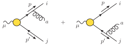
Figure 14: Diagrams for the radiation of a single gluon from a generic hard scattering vertex producing a $q\bar{q}$ pair.

We can now be more precise in defining the soft approximation: we rescale all components of the gluon momentum $k$ as

$$k^{\mu}\,\to\,\lambda k^{\mu}\,,\qquad\quad\lambda\,\to\,0\,,$$ (2.34)

and retain only the leading power in the Laurent expansion in powers of $\lambda$. For the amplitude in Eq. (2.33), the only effect of this approximation is to drop terms proportional to $k^{\mu}$ in the numerator. Then, as was done in Section 1.1, we can use the Dirac equation, after commuting $p\hskip-4.49997pt/_{1}$ and $p\hskip-4.49997pt/_{2}$ across $\varepsilon\hskip-4.49997pt/(k)$, to get

$${\cal A}^{\mu\,a}_{ij}\,=\,g\,T^{a}_{ij}\,\left(\frac{p_{1}\cdot\varepsilon}{p_{1}\cdot k}-\frac{p_{2}\cdot\varepsilon}{p_{2}\cdot k}\right){\cal A}^{\mu}_{\rm Born}\,+\,{\cal O}(k^{0})\,\equiv\,{\cal S}^{a}_{ij}\,{\cal A}^{\mu}_{\rm Born}\,+\,{\cal O}(k^{0})\,,$$ (2.35)

where ${\cal A}^{\mu}_{\rm Born}\equiv\overline{u}(p_{1})\Gamma^{\mu}v(p_{2})$. It is worthwhile pausing briefly to note the properties of the soft amplitude ${\cal S}^{a}_{ij}\,{\cal A}^{\mu}_{\rm Born}$, which will generalise to higher orders.

• The soft amplitude is gauge-invariant, as can be seen by picking a longitudinal polarisation vector $\varepsilon^{\mu}\propto k^{\mu}$.

• The soft amplitude is universal, in the sense that it does not depend upon the spin of the hard particles (which has been factored into the Born term), nor does it depend on their energy: indeed, the soft factor ${\cal S}^{a}_{ij}$ is homogeneous in the hard momenta $p_{1}$ and $p_{2}$, so that in fact it is only sensitive to their direction and not to their magnitude. One may rescale the momenta setting $p_{i}^{\mu}=Q\,\beta_{i}^{\mu}$, and the soft factor will depend only on the ‘four-velocities’ $\beta_{i}$.

• The soft amplitude can be interpreted as the action of a soft colour operator ${\cal S}^{a}_{ij}$ on the Born amplitude, which is colour-diagonal in the fundamental representation, since the hard vertex is a colour-singlet.

• Squaring the soft amplitude and summing over $N_{c}$ colours we get a differential cross section proportional to

  $$\sum_{\rm pol}\sum_{\rm col}\left|{\cal S}^{a}_{ij}\;{\cal A}^{\mu}_{\rm Born}\right|^{2}\,=\,g^{2}\,N_{c}\,C_{F}\,\left|{\cal A}^{\mu}_{\rm Born}\right|^{2}\frac{2\beta_{1}\cdot\beta_{2}}{\beta_{1}\cdot k\,\beta_{2}\cdot k}\,,$$ (2.36)

  which, as expected, is proportional to the Born cross section, and correctly reproduces the soft (though not the collinear) singularities of the full radiative cross sections computed from Eq. (2.33).

A similar, slightly more complicated analysis (see Section 4) shows that a factorisation of this kind happens also in the two collinear limits: in that case, the collinear factorisation kernel is a colour singlet, but, in general, a spin matrix acting on the Born amplitudes. Once again, in the singular limit, one finds a result proportional to the Born cross section, which enables the KLN cancellation of singularities.

Since the cancellation of singularities happens locally in the radiative phase space, as stated by the KLN theorem, in order to construct a safe observable it must be sufficient to integrate the radiation only over a neighbourhood of the singular regions (soft and collinear configuration). This has led to the definiton and usage of weighted cross sections, or event shapes: one proceeds by defining a potential observable in the $m$-particle phase space as a function $E_{m}(p_{1},\ldots,p_{m})$; one then computes the distribution for that observable by weighing all possible final states with that function, as

$$\frac{d\sigma}{de}\,=\,\frac{1}{2q^{2}}\sum_{m}\int d\Phi_{m}\,\overline{\left|{\cal A}_{m}\right|^{2}}\,\delta\big{(}e-E_{m}(p_{1},\ldots,p_{m})\big{)}\,,$$ (2.37)

where $\Phi_{m}$ is the Lorentz-invariant phase space for the $m$ particles carrying momenta $p_{i}$, $i=1,\ldots,m$, and ${\cal A}_{m}$ is the corresponding amplitude. The cancellation of infrared singularities will happen, to all orders in perturbation theory, if the chosen function $E_{m}$ is insensitive to soft and collinear radiation, so that final states that differ by such radiation are weighted equally. The precise requirement is

$$\lim_{p_{i}\to 0}\,E_{m+1}\big{(}p_{1},\ldots,p_{i},\ldots,p_{m+1}\big{)} = E_{m}\big{(}p_{1},\ldots,p_{i-1},p_{i+1},\ldots,p_{m+1}\big{)}\,,$$

$$\lim_{p_{i}\parallel\,p_{j}}\,E_{m+1}\big{(}p_{1},\ldots,p_{i},\ldots,p_{j},\ldots p_{m+1}\big{)} = E_{m}\big{(}p_{1},\ldots,p_{i}+p_{j},\ldots,p_{m+1}\big{)}\,,$$ (2.38)

defining an infrared-safe, or soft-collinear-safe observable [238, 239]. Jet cross sections in e⁺ e^- annihilation belong to this category, where the functions $E_{m}$ are, for example, sets of step functions that force soft and collinear radiation to be integrated over [240], while hard partons are ‘measured’ (so that the observable $e$ becomes a collection of energies and angles); alternatively $E_{m}$ can be defined iteratively, building up an (infrared-safe) jet algorithm (see, for example [241]).

2.7 A tool: eikonal integrals

As discussed above, the soft approximation for real radiation is a fairly straightforward affair: it basically amounts to a Laurent expansion in the soft momentum, where, by picking the leading power, one locates the soft singularities and uncovers interesting universality properties. Not surprisingly, the situation is significantly more intricate when it comes to taking the soft approximation for virtual corrections, where the soft momentum is an integration variable. The soft limit and the loop integration do not commute, and things must be handled with care. In order to illustrate the problems that arise, consider taking the soft limit, at the level of the integrand, on the scalar integral $I_{0}$ defined in Eq. (2.21), which is responsible for the soft poles of the form factor. Applying Eq. (2.34), and restoring the prefactors arising from the Feynman rules and from the colour sum, we define

$$I_{\rm eik}\,\equiv\,{\rm i}g^{2}\mu^{2\epsilon}\,N_{c}\,C_{F}\,\beta_{1}\cdot\beta_{2}\int\frac{d^{d}k}{(2\pi)^{d}}\,\frac{1}{\left(k^{2}+{\rm i}\eta\right)\left(-\beta_{1}\cdot k+{\rm i}\eta\right)\left(\beta_{2}\cdot k+{\rm i}\eta\right)}\,,$$ (2.39)

By inspection, there are several things to note about Eq. (2.39).

• As expected, also in the case of virtual corrections the soft approximation is independent of spin and energy: the integral is homogeneous in both external momenta, and thus depends only on the dimensionless four-velocities $\beta_{i}$.

• The integral is highly singular, in a rather intricate way: it is simultaneously affected by ultraviolet, soft and collinear divergences. Before even attempting to evaluate it, it will be necessary to understand the origin of the different singularities, and how to treat them.

• On the other hand, while highly singular, $I_{\rm eik}$ is readily ‘evaluated’ in dimensional regularisation: since it does not depend on any scale, it is defined to vanish.

The proper way to handle this vanishing integral emerges upon studying the nature of its singularities. First of all, as should be clear from the analysis of Section 2.4, we observe that the UV divergence of $I_{\rm eik}$ is not inherited from QCD: indeed, the UV divergence of the original QCD diagram is completely contained in the tensor integral $I^{\alpha\beta}$. The fact is, taking the limit in Eq. (2.34), we have constructed an integrand which is a good approximation of the form factor integrand in the region $k^{\mu}\to 0$, but a very poor approximation in the UV region $k^{\mu}\to\infty$. As a consequence, our ‘effective low-energy theory’ for the form factor has developed a new UV divergence, and, if we want to recover the proper low-energy result, we need to subtract (renormalise) this spurious UV pole. In other words, the physics we are seeking to control is not to be found in the ‘bare’ version of $I_{\rm eik}$, with which we have been working so far, but in the renormalised quantity

$$I_{\rm eik}^{({\rm R})}\,=\,I_{\rm eik}+I_{\rm eik}^{({\rm ct})}\,=\,I_{\rm eik}^{({\rm ct})}\,,$$ (2.40)

where $I_{\rm eik}^{({\rm ct})}$ is the UV counterterm, and we have used the fact that $I_{\rm eik}=0$. What needs to be done is now clear: we need to introduce auxiliary regulators to make the original $I_{\rm eik}$ integral finite in the soft and collinear regions; this will hopefully allow to unambiguously compute the UV pole; we then take the (minimal subtraction) UV counterterm as the the definition of $I_{\rm eik}^{({\rm R})}$, as in Eq. (2.40). Using a minimal scheme is essential in order to avoid dependence on the auxiliary regulators.

A detailed and consistent technique to perform this sequence of operations at high orders in the loop expansion will be presented in Section 5.3 (see Ref. [242]). For a simple integral such as $I_{\rm eik}$, where all singular regions are easily identified, this is not needed, and we can get the right result by a sleight of hand. Proceed by introducing Feynman parameters in two steps: first combining the two linear denominators in $I_{\rm eik}$ with parameter $x$, and then combining the resulting (squared) denominator with the gluon propagator, with parameter $y$. One finds

$$I_{\rm eik} = {\rm i}g^{2}\mu^{2\epsilon}\,N_{c}\,C_{F}\,\beta_{1}\cdot\beta_{2}\int_{0}^{1}\!dx\int_{0}^{1}\!dy\int\frac{d^{d}k}{(2\pi)^{d}}\,\frac{2(1-y)}{\Big{[}yk^{2}+(1-y)\big{(}x\beta_{2}-(1-x)\beta_{1}\big{)}\cdot k+{\rm i}\eta\Big{]}^{3}}$$ (2.41)

$$= -\frac{\alpha_{s}}{2\pi}\left[\frac{8\pi\mu^{2}}{-\beta_{1}\cdot\beta_{2}-{\rm i}\eta}\right]^{\epsilon}\,N_{c}\,C_{F}\,\Gamma(1+\epsilon)\,B\left(-\epsilon,-\epsilon\right)\,\int_{0}^{1}dy\,y^{-1+2\epsilon}\,(1-y)^{-1-2\epsilon}\,.$$

The pole in $B\left(-\epsilon,-\epsilon\right)=-2/\epsilon+{\cal O}(\epsilon)$ is of collinear origin: one can see this by noting that it arises from the $x$ integration, and the corresponding singular regions in Feynman-parameter space are $x\to\{0,1\}$; the limit $x\to 0$ in the first line of Eq. (2.41) exposes the collinear singularity as $k^{\mu}\propto\beta_{1}$, which implies also $k^{2}\to 0$; similarly, the limit $x\to 1$ exposes the collinear singularity as $k^{\mu}\propto\beta_{2}$. Next, one may be tempted to replace the last integral in Eq. (2.41) with $B(2\epsilon,-2\epsilon)=0$. This looks consistent with the definition of the integral in dimensional regularisation, but actually it merely reminds us that the original integral is not well-defined for any values of $\epsilon$: it is plagued by either UV or soft divergences in any dimension. Once again, it is simple in this case to identify and disentangle the UV pole, which we are interested in. Looking at the integrand in the first line of Eq. (2.41), we see that the limit $y\to 0$ exposes a UV singularity (the integral diverges as $k^{\mu}\to\infty$ when $y=0$), and is correspondingly regulated by taking $\epsilon>0$. Conversely, the limit $y\to 1$ exposes an IR singularity (the integral diverges as $k^{\mu}\to 0$ for $y\to 1$), and is correspondingly regulated by taking $\epsilon<0$. The two singular regions can be separated by inserting a factor of $1=y+(1-y)$, getting

$$\int_{0}^{1}dy\,y^{-1+2\epsilon}\,(1-y)^{-1-2\epsilon} = \int_{0}^{1}dy\,y^{-1+2\epsilon}\,(1-y)^{-1-2\epsilon}\,\left[y+(1-y)\right]$$ (2.42)

$$= \Gamma(1+2\epsilon)\Gamma(-2\epsilon)+\Gamma(2\epsilon)\Gamma(1-2\epsilon)\,.$$

The second term in Eq. (2.42) gives the UV pole, so that the one-loop counterterm in the MS scheme is

$$I_{\rm eik}^{({\rm R})}\,=\,I_{\rm eik}^{({\rm ct})}\,=\,-\frac{\alpha_{s}}{2\pi}\,N_{c}\,C_{F}\,\frac{1}{\epsilon}\left[\frac{1}{\epsilon}-\gamma_{E}+\ln(4\pi)+\ln\left(\!-\frac{\beta_{1}\cdot\beta_{2}}{2}\right)\right]\,.$$ (2.43)

Three observations are in order.

• The overall $1/\epsilon$ pole in Eq. (2.43) is of ultraviolet origin. The pole in the square bracket is the collinear divergence: if the hard partons were massive, it would be replaced by a logarithm of the Minkowskian angle between the two parton velocities, as discussed in detail in Section 5.3.

• The UV pole in Eq. (2.43), which is the UV pole of $I_{\rm eik}$ with the opposite sign, can be directly interpreted as a soft singularity. The coefficient of the ensuing double (soft-collinear) pole is the one-loop contribution to anomalous dimension associated with this UV divergence, which we will identify, in Section 4, with the QCD light-like cusp anomalous dimension [243, 244].

• In the presence of the collinear singularity, the rescaling symmetry of $I_{\rm eik}$ under $\beta_{i}\to\kappa_{i}\beta_{i}$ is broken by the logarithmic term in Eq. (2.43), which multiplies the ultraviolet pole and thus cannot be discarded. This ‘anomalous’ breaking of rescaling invariance will have very significant consequences for the structure of IR divergences of multi-parton amplitudes, to be discussed in Section 5.

Most of the discussion in this section so far has focussed on the soft limit. Before turning, in Section 3, to the all-order generalisation of the one-loop results presented here, we briefly recall what happens in the presence of collinear divergences, when the Bloch-Nordsieck cancellation does not suffice, and one needs to resort to collinear factorisation.

2.8 Hadron scattering and collinear divergences

For the sake of completeness, in this Section we sketch the one-loop calculation of Deep Inelastic Scattering (DIS) structure functions, the classic example of non-cancellation of infrared divergences in QCD, due to the presence of initial-state hadrons, and the starting point of the factorisation program. The calculation is of course well known, so we only briefly summarise it, and we focus on the origin and the treatment of uncanceled divergences, to be compared with Section 2.3 and Section 2.4. We consider lepton-proton scattering via photon exchange, neglecting masses, and specifically we focus on scattering off valence quarks, involving the diagrams displayed in Fig. 15-16 at LO and NLO.

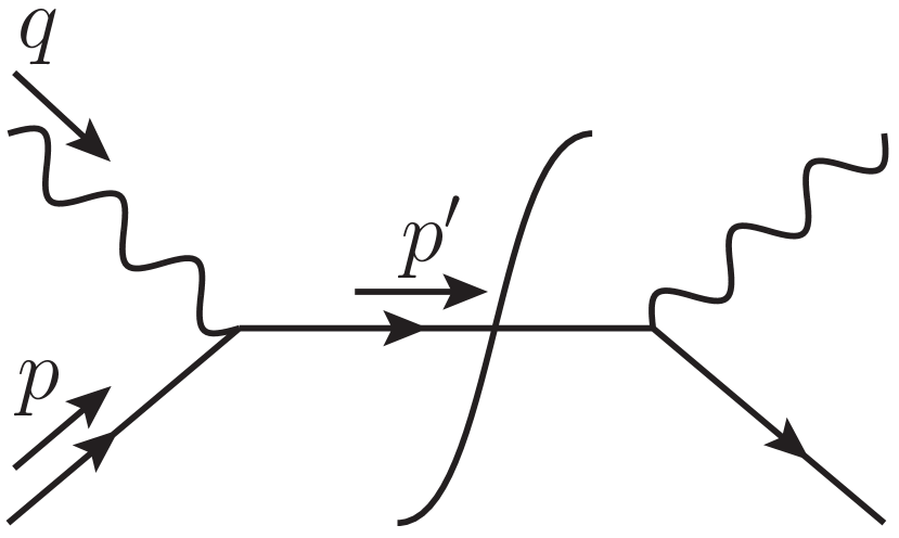
(a)

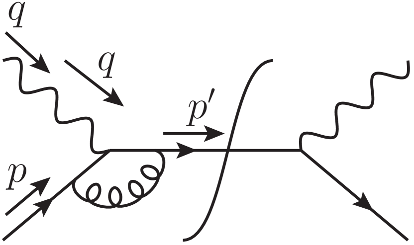
(b)

Figure 15: Leading-order and virtual correction diagrams for Deep Inelastic Scattering (DIS) up to order $\alpha_{s}$ (self-energy diagrams are omitted).

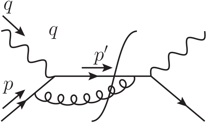
(a)

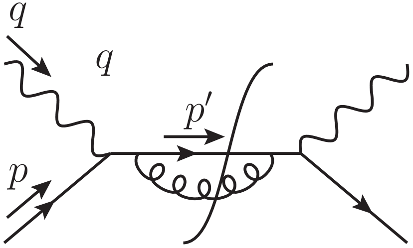
(b)

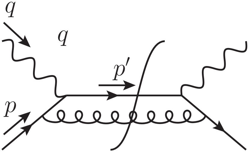
(c)

Figure 16: Real-radiation diagrams for the DIS cross section at order $\alpha_{s}$.

We assign momentum $l$ to the incoming lepton, momentum $l^{\prime}$ to the outgoing lepton, and momentum $p$ to the incoming hadron, and we employ the usual conventions for kinematic variables

$$q^{\mu}\,\equiv\,\big{(}l^{\prime}-l\big{)}^{\mu}\,,\qquad-q^{2}\,\equiv\,Q^{2}\,>\,0\,,\qquad x\,\equiv\,\frac{Q^{2}}{2p\cdot q}\,\rightarrow\,s\,\equiv\,(p+q)^{2}\,=\,Q^{2}\,\frac{1-x}{x}\,.$$ (2.44)

In analogy with Eq. (2.2), we can factor the cross section for this process into the product of leptonic and hadronic tensors. For the spin-averaged differential cross section we write then

$$d^{3}\sigma\,=\,\frac{1}{2s}\,\frac{d^{3}l^{\prime}}{(2\pi)^{3}2E^{\prime}}\,L^{\mu\nu}(l,l^{\prime})\,W_{\mu\nu}(p,q)\,$$ (2.45)

where $E^{\prime}=|{\bf l}^{\prime}|$, and, to leading order in the lepton charge, the lepton tensor (defined to include photon propagators) simply reads

$$L^{\mu\nu}\,\equiv\,\frac{e^{2}}{Q^{4}}\,\,{\rm Tr}\Big{(}\not{l}\,\gamma^{\mu}\,\not{l}^{\prime}\,\gamma^{\nu}\Big{)}\,.$$ (2.46)

In analogy to what we did for the annihilation cross section in Eq. (2.4), we can express the hadronic tensor $W_{\mu\nu}$ in terms of matrix elements of the electromagnetic current in the relevant hadron state. For a particle of electric charge $eQ_{f}$ we write

$$W_{\mu\nu}(p,q) = \frac{e^{2}Q_{f}^{2}}{8\pi}\sum_{{\rm spin},\,X}\,\left\langle\smash{p}{\vphantom{1}}\right|J_{\mu}^{\dagger}(0)\left|\smash{X}{\vphantom{1}}\right\rangle\left\langle\smash{X}{\vphantom{1}}\right|J_{\nu}(0)\left|\smash{p}{\vphantom{1}}\right\rangle\,(2\pi)^{4}\,\delta^{4}(p_{X}-q-p)$$ (2.47)

$$= \frac{e^{2}Q_{f}^{2}}{8\pi}\,\sum_{\rm spin}\int d^{4}x\,{\rm e}^{{\rm i}q\cdot x}\,\left\langle\smash{p}{\vphantom{1}}\right|J_{\mu}^{\dagger}(x)\,J_{\nu}(0)\left|\smash{p}{\vphantom{1}}\right\rangle\,.$$

Lorentz covariance, gauge invariance and parity conservation constrain the tensor structure to be of the form

$$W_{\mu\nu}(p,q)\,=\,-\bigg{(}g_{\mu\nu}-\frac{q_{\mu}q_{\nu}}{q^{2}}\bigg{)}F_{1}(x,Q^{2})+\frac{1}{p\cdot q}\bigg{(}p_{\mu}-q_{\mu}\frac{p\cdot q}{q^{2}}\bigg{)}\bigg{(}p_{\nu}-q_{\nu}\frac{p\cdot q}{q^{2}}\bigg{)}F_{2}(x,Q^{2})\,,$$ (2.48)

and one easily verifies that, if the state $\left|\smash{p}{\vphantom{1}}\right\rangle$ in Eq. (2.47) is a massless spin $1/2$ fermion, at tree level one finds the elastic scattering result

$$F_{2}^{(0)}(x,Q^{2})\,=\,2F_{1}^{(0)}(x,Q^{2})\,=\,e^{2}Q_{f}^{2}\,\delta(1-x)\,,$$ (2.49)

famously exhibiting scaling behavior [245], i.e. independence on the scale $Q^{2}$, which is a hallmark of the parton model [246], and was experimentally verified at SLAC half a century ago [247].

At NLO, the infrared content of the process becomes non-trivial. Since we know that $W_{\mu\nu}$ is built out of only two independent scalar functions, it is sufficient to compute the contractions of the hadronic tensor with $g_{\mu\nu}$ and with $p_{\mu}p_{\nu}$. For our purposes, the interesting quantity is the trace of the hadronic tensor, $W\equiv-g^{\mu\nu}W_{\mu\nu}$, which contains the non-trivial infrared information. Looking at the virtual diagrams in Fig 15, panel (b), one realises that they build up the quark form factor, Eq. (2.22), this time for space-like kinematics, as can be expected. The precise result is

$$W_{\rm virt}^{(1)}(p,q) = 2\,{\bf Re}\left[\Gamma^{(1)}\bigg{(}\frac{Q^{2}}{\mu^{2}},\epsilon\bigg{)}\right]W^{(0)}\,=\,2\,{\bf Re}\left[\Gamma^{(1)}\bigg{(}\frac{Q^{2}}{\mu^{2}},\epsilon\bigg{)}\right](1-\epsilon)\,e^{2}Q_{f}^{2}\,\delta(1-x)$$

$$= -\frac{\alpha_{s}}{2\pi}\,C_{F}\bigg{(}\frac{4\pi\mu^{2}}{Q^{2}}\bigg{)}^{\!\epsilon}\,\frac{\Gamma^{2}(1-\epsilon)\,\Gamma(1+\epsilon)}{\Gamma(1-2\epsilon)}\bigg{(}\frac{2}{\epsilon^{2}}+\frac{3}{\epsilon}+8\bigg{)}\,(1-\epsilon)\,e^{2}Q_{f}^{2}\,\delta(1-x)\,,\qquad$$

where in the first line we used the explicit expression for the tree-level trace of the hadronic tensor, $W^{(0)}$, easily derived from Eq. (2.48) and Eq. (2.49). Motivated by our success in cancelling infrared poles in Section 1.1 and in Section 2.1, we can now compute the cross section for the emission of a real gluon with momentum $k$. The contribution to the trace of the hadronic tensor, in analogy to Eq. (2.11), is

$$W_{\rm real}^{(1)}(p,q) = \frac{1}{8\pi}\int\frac{d^{d}p^{\prime}d^{d}k}{(2\pi)^{d-2}}\,\delta^{d}(p+q-p^{\prime}-k)\,\delta_{+}(p^{\prime\,2})\,\delta_{+}(k^{2})\,\Big{|}{\cal A}(p,q,k)\Big{|}^{2}\,,$$ (2.51)

where $|{\cal A}(p,q,k)|^{2}$ is a short-hand notation for the square of the real-radiation matrix element, summed over final state colours and polarisations, averaged over initial-state colour, and traced over the open photon indices. ${\cal A}$ now characterises a $2\to 2$ process, with the Mandelstam invariant $s$ given by Eq. (2.44), while

$$t\,=\,(p-k)^{2}\,=\,-2p\cdot k\,,\quad u\,=\,(p-p^{\prime})^{2}\,=\,-2p\cdot p^{\prime}\quad\rightarrow\quad s+t+u\,=\,-Q^{2}\,.$$ (2.52)

In $d=4-2\epsilon$, one finds

$$\Big{|}{\cal A}(p,q,k)\Big{|}^{2}\,=\,32\pi\,e^{2}Q_{f}^{2}\,\alpha_{s}^{2}\mu^{2\epsilon}\,C_{F}\,(1-\epsilon)\bigg{[}(1-\epsilon)\bigg{(}\frac{s}{-t}+\frac{-t}{s}\bigg{)}+\frac{2Q^{2}u}{st}+2\epsilon\bigg{]}\,.$$ (2.53)

In order to perform the integrals in Eq. (2.51), it is useful to parametrise the invariants as

$$t\,=\,-\frac{Q^{2}}{x}(1-y)\,,\qquad u\,=\,-\frac{Q^{2}}{x}y\,,$$ (2.54)

where $y$ plays the role of an angular variable, as in Eq. (2.14): in the collinear limit $y\to 1$ and $t\to 0$, and the squared matrix element in Eq. (2.53) displays the expected collinear singularity. Performing the phase space integrals in Eq. (2.51), with the help of Eq. (2.12) and Eq. (2.13), one finally finds

$$W_{\rm real}^{(1)}(p,q) = e^{2}Q_{f}^{2}\,\,\frac{\alpha_{s}}{2\pi}C_{F}\,\bigg{(}\frac{4\pi\mu^{2}}{s}\bigg{)}^{\!\epsilon}\,\frac{\Gamma(2-\epsilon)}{\Gamma(1-2\epsilon)}\bigg{[}-\frac{1}{\epsilon}\,\frac{1+x^{2}}{1-x}-\frac{3+\epsilon}{2(1-2\epsilon)}\,\frac{1}{1-x}$$

$$\hskip 184.9429pt+\,\frac{2(1-2\epsilon^{2})}{(1-\epsilon)(1-2\epsilon)}+(1-x)\bigg{]}\,.$$

Had one expected a cancellation of the singularities of Eq. (2.8), Eq. (2.8) would be a striking disappointment, displaying no obvious double pole, and a single pole with non-trivial dependence on $x$. Let’s look at these two aspects in turn.

Considering first the soft singularity, we note that the soft limit $k^{\mu}\to 0$ coincides with the elastic scattering limit $x\to 1$: the soft singularity is present, but it is localised at $x=1$. In order to emphasise this, we first express the prefactor in Eq. (2.8) in terms of the scale $Q^{2}$, using Eq. (2.44): this turns the factors of $(1-x)^{-1}$ into $(1-x)^{-1-\epsilon}$, regularising the $x\to 1$ singularity for $\epsilon<0$, as expected. We then proceed to interpret this factor in terms of distributions, noting that integrals of the form

$$I(f)\,=\,\int_{0}^{1}dx\,(1-x)^{-1-\epsilon}f(x)\,,$$ (2.56)

for any function $f(x)$ regular at $x\to 1$, can be computed as power series in $\epsilon$ using

$$I(f) = \int_{0}^{1}dx\,\frac{f(x)-f(1)}{(1-x)^{1+\epsilon}}+f(1)\int_{0}^{1}dx\,\frac{1}{(1-x)^{1+\epsilon}}$$ (2.57)

$$= -\frac{1}{\epsilon}f(1)\,+\,\sum_{n=0}^{\infty}\,(-1)^{n}\,\frac{\epsilon^{n}}{n!}\int_{0}^{1}dx\,\frac{\ln^{n}(1-x)}{1-x}\,\big{(}f(x)-f(1)\big{)}\,.$$

Introducing the distributions

$${\cal D}_{n}(x)\,\equiv\,\left[\frac{\ln^{n}(1-x)}{1-x}\right]_{+}\,\rightarrow\,\,\int_{0}^{1}dx\,{\cal D}_{n}(x)f(x)\,\equiv\,\int_{0}^{1}dx\,\frac{\ln^{n}(1-x)}{1-x}\,\big{(}f(x)-f(1)\big{)}\,,$$ (2.58)

one can formalise Eq. (2.57) in terms of the distribution identity

$$\frac{1}{(1-x)^{1+p\epsilon}}\,=\,-\frac{1}{p\epsilon}\,\delta(1-x)\,+\,\sum_{n=0}^{\infty}\,(-1)^{n}\,\frac{(p\epsilon)^{n}}{n!}\,{\cal D}_{n}(x)\,.$$ (2.59)

Substituting Eq. (2.59) in the pole term of Eq. (2.8) we immediately see that a double pole proportional to $\delta(1-x)$ is generated, and indeed it cancels the double pole of Eq. (2.8). Discarding contributions of order $\epsilon$, the final result for the trace of the hadronic tensor can be written as

$$W^{(1)}(p,q)\,=\,\frac{\alpha_{s}}{2\pi}\,\bigg{(}\frac{4\pi\mu^{2}}{Q^{2}}\bigg{)}^{\epsilon}\,e^{2}Q_{f}^{2}\,(1-\epsilon)\bigg{[}-\frac{1}{\epsilon}\,\frac{\Gamma(1-\epsilon)}{\Gamma(1-2\epsilon)}\,P_{qq}(x)+$$ (2.60)

$$\hskip 14.22636pt+\,C_{F}\bigg{(}\big{(}1+x^{2}\big{)}{\cal D}_{1}(x)-\frac{3}{2}\,{\cal D}_{0}(x)-(1+x^{2})\,\frac{\log x}{1-x}+3-x-\Big{(}\frac{9}{2}+\frac{\pi^{2}}{3}\Big{)}\delta(1-x)\bigg{)}\bigg{]},$$

where we introduced the leading-order DGLAP splitting function [248, 249, 250]

$$P_{qq}(x)\,=\,C_{F}\bigg{[}(1+x^{2})\,{\cal D}_{0}(x)+\frac{3}{2}\,\delta(1-x)\bigg{]}\,,$$ (2.61)

with the virtual term normalised so that $\int_{0}^{1}dxP_{qq}(x)=0$. While the splitting function was derived here in the context of DIS, it is a universal quantity, and we will discuss it further, and give a process-independent derivation, in Section 6.1.

After the cancellation of the soft singularity, Eq. (2.60) is left with a single pole, which is manifestly of collinear nature (since it has support for $x\neq 1$). It is important to note at the outset that this pole has nothing to do with the non-abelian nature of the interaction, and certainly nothing to do with confinement: indeed, precisely the same pole would arise in the abelian theory, for example in the scattering of a massless charged fermion from a classical source. In ordinary QED, the singularity is regularised by the electron mass, but this is of little help for perturbative calculations at large momentum transfer, since the pole is replaced at each order by large logarithms of the ratio $m_{e}/Q$, which spoil the behaviour of the perturbative series unless they are resummed. Let us then discuss the origin and treatment of this collinear singularity in light of the results of Section 1.2 and Section 1.3.

To understand the failure of the Bloch-Nordsieck mechanism, it helps to compare the DIS process to the total annihilation cross section, considering the relevant diagrams in the context of time-ordered perturbation theory. For the real emission diagrams in Fig. 11, the dominant time ordering for the emission of soft or collinear gluons is the one where the current creates the quark pair at time $t_{c}$, and the gluon is radiated at time $t_{r}\gg t_{c}$. Crucially, this late-time emission does not affect the Born process, which still consists of the creation of a pair with total energy $Q$. As the virtual correction is always proportional to the Born process, the cancellation of singularities is at least possible. In DIS kinematics, on the other hand, the dominant time ordering for collinear emission in the ‘handbag’ diagram of Fig. 16(c) is the one in which gluon radiation takes place at time $t_{r}\ll t_{c}$: the current therefore scatters a quark with an energy different from that of the Born process, which is reflected by the fact that $x\neq 1$. Only when the radiated gluon is soft one recovers the elastic configuration, and the cancellation of divergences with the virtual correction becomes possible.

Any treatment of this problem must rely on the understanding that gluon (or photon) emission at very early times is not to be associated with the hard scattering process, but rather with the wave function of the initial state. Indeed, as we saw in Section 1.3.1, in the coherent-state picture the collinear singularity is cancelled by a contribution in which the radiation originates from the initial-state coherent state operator; analogously, applying the KLN theorem requires in this case a sum over degenerate initial states. The inescapable conclusion is that a massless particle in the initial state must always be understood as a beam, containing different Fock state components. In general, different components should be evaluated at amplitude level, and will interfere at cross-section level; at large momentum transfer, the statement of collinear factorisation is that interference terms are suppressed by powers of the hard scale, and one is allowed to sum incoherently over different channels, weighted by the respective probabilities.

We will not discuss techniques to prove factorisation here: they will be introduced, at the level of scattering amplitudes, in Sections 3, 4 and 5, and they have been thoroughly presented elsewhere (see, for example, Ref. [60]). We take however the opportunity to make the qualitative arguments of Section 1.4.2 slightly more precise. Consider a DIS-type process initiated by a massless particle of flavour $i$, which has lagrangian interactions with a set of massless particles with flavours $\{j\}$. Initial-state radiation can turn particle $i$ into any other particle $j$ (including of course the case $j=i$), with a degraded longitudinal momentum, and one can define a probability distribution $f_{j/i}(z,\epsilon)$ for detecting particle $j$ as a ‘constituent’ of particle $i$, carrying a fraction $z$ of the longitudinal momentum of $i$. Such distributions can be constructed by means of (non-local) matrix elements of field operators in the single-particle state containing particle $i$ [251, 60, 2, 61, 67], in order to reproduce the collinear divergences of the hadronic tensor. Even without resorting to a formal definition, it is easy to illustrate the mechanics of the factorisation procedure: any projection of the hadronic tensor $W^{\mu\nu}_{i}$ for the process initiated by particle $i$ can be written as

$$W_{i}(p,q)\,=\,\sum_{j}\int_{0}^{1}\frac{dz}{z}\,H_{j}(zp,q)\,f_{j/i}(z,\epsilon)\,,$$ (2.62)

with the goal of defining a set of collinear-finite hard functions $H_{j}$. At tree level, with no emissions, one can normalise the hadronic tensor (dropping coupling factors) so that

$$W_{i}^{(0)}(p,q)\,=\,\delta(1-x)\,,\!\quad\!f_{j/i}^{(0)}(z,\epsilon)\,=\,\delta_{ij}\delta(1-z)\!\quad\!\rightarrow\quad H_{j}^{(0)}(zp,q)\,=\,\delta\left(1-\frac{x}{z}\right)\,.$$ (2.63)

It is then straightforward to expand Eq. (2.62) to NLO, with the result

$$W_{i}^{(1)}(p,q)\,=\,\sum_{j}f_{j/i}^{(1)}(x,\epsilon)+H_{i}^{(1)}(p,q)\,.$$ (2.64)

One sees that divergent contributions such as those emerging in Eq. (2.60) can be collected as radiative corrections to the parton distributions $f_{j/i}(x,\epsilon)$; furthermore, one is free to choose a factorisation scheme, by assigning sets of nonsingular contributions to either $f_{j/i}$ of $H_{i}$. The subsequent interpretation and usage of Eq. (2.64) and its higher-order generalisations will depend on the context. In a confining theory such as QCD, the perturbative parton distribution $f_{j/i}$ must be convoluted with its hadronic counterpart, which is non-perturbative and needs to be determined experimentally. In the case of QED, on the other hand, it is natural to replace the dimensional regulator with the physical one – the mass of the charged particle: the distributions $f_{j/i}$ are then computable in perturbation theory [252, 253]. In either case, the most striking consequence of Eq. (2.60) is the breaking of the scale invariance that was observed at tree level in Eq. (2.49). Upon expanding Eq. (2.60) in powers of $\epsilon$, and after removing the collinear pole to the parton distribution, one observes a logarithmic dependence on the hard scale $Q$, with a coefficient given by the splitting kernel $P_{qq}$. We note now a pattern which will be recurring in the following Sections (see, in particular, the discussion at the beginning of Section 4): once a factorisation, such Eq. (2.62), is achieved, extracting contributions that are singular as the regulator is removed entails the choice of a factorisation scale, $\mu_{f}$, separating long-distance and short-distance contributions. In the present case, the scale $\mu_{f}$ can be introduced simply by splitting the logarithm emerging from Eq. (2.60) as

$$\ln\left(\frac{\mu^{2}}{Q^{2}}\right)\,=\,\ln\left(\frac{\mu^{2}}{\mu_{f}^{2}}\right)\,+\,\ln\left(\frac{\mu_{f}^{2}}{Q^{2}}\right)\,;$$ (2.65)

one then assigns the first term to the parton distribution, which is taken to depend on energy scales below $\mu_{f}$, and the second term to the hard function, which retains the dependence on the hard scale $Q$.

As we will discuss in greater detail in Section 4, this artificial scale separation inevitably leads to the existence of an evolution equation, following from the requirement that physical quantities be independent of the arbitrary scale choice. The solution to this equation will resum scale logarithms, in this case of collinear origin. At our present accuracy, using the tree-level result in Eq. (2.63), and applying Eq. (2.65), one immediately verifies that the one-loop distribution satisfies the DGLAP equation

$$\mu_{f}^{2}\frac{\partial}{\partial\mu_{f}^{2}}\,f_{q/q}\big{(}x,\mu_{f}^{2}\big{)}\,=\,\frac{\alpha_{s}}{2\pi}\int_{x}^{1}\frac{dy}{y}\,P_{qq}\left(\frac{x}{y},\alpha_{s}\right)f_{q/q}\big{(}y,\mu_{f}^{2}\big{)}\,,$$ (2.66)

where Eq. (2.61) gives the leading order approximation to the kernel $P_{qq}$, and the lower limit of integration reflects the fact that collinear radiation can only degrade the longitudinal momentum fraction. Both in QED [254, 255, 256, 257, 258, 259] and in QCD [248, 249, 250], the resummation of collinear logarithms that follows from solving DGLAP equations like Eq. (2.66) is a crucial step in order to obtain accurate predictions for high-energy processes [238].

For inclusive DIS, the validity of the factorisation in Eq. (2.62) to all orders in perturbation theory can be established both with diagrammatic methods [2, 67] and using the Operator Product Expansion (OPE) [1]. The generalisation to collider processes, involving two hadrons in the initial state, is both conceptually and technically non trivial. Physically, one could readily imagine that, in a collider process, as the two colliding hadrons approach, colour forces from one hadron might alter the parton configuration of the second one, spoiling the universality of the distributions measured in single-hadron process. Soft gluons, with their long wavelength, are prime candidates to be responsible for this failure of factorisation. In a general collider process, the OPE is not available, and establishing the cancellation of such soft-gluon effects to all orders in perturbation theory is a delicate exercise [260, 261, 262, 204, 205], reviewed in Ref. [60]. Such factorisation proofs require an all-order analysis of Feynman diagrams: we now turn to describing some of the tools required to perform these studies.

3 Infrared singularities to all orders

The discussion in Section 2 was mostly limited to the lowest non-trivial perturbative order – one loop. Here we prepare the ground for studying the problem to all orders. Superficially, the complexity of the problem appears daunting – how can one disentangle the structure of singularities of arbitrarily intricate Feynman diagrams, and organise them in an intelligible pattern? We can find some hope in the successful treatment of QED in Section 1.1, which suggests that infrared singularities are perhaps relatively simple, as they are constrained by their semi-classical nature and by their origin in long-distance dynamics. This hope is indeed well founded: research developed over several decades has in fact, to a large extent, succeeded in uncovering the all-order infrared structure of perturbative non-abelian gauge theories, as we will see in some detail in Sections 4 and 5.

Factorisation and exponentiation of soft and collinear singularities can be achieved in four steps. First, one needs to locate potential singularities in generic Feynman integrals, establishing necessary conditions for singularities to arise. These conditions are summarised by the Landau equations, discussed below in Section 3.1. Next, one needs to ascertain in what cases the solutions of Landau equations yield actual singularities, establishing sufficient conditions for Feynman integrals to diverge. While the necessary conditions are largely universal, sufficient conditions are theory-specific, and require the development of power-counting tools, similar to the ones used for the renormalisation of ultraviolet divergences. These tools are discussed in Section 3.2. The third step leverages the universality of infrared singularities and their long-distance character by constructing operator matrix elements, independent of the hard scattering process being considered, and yet capable of reproducing the leading-power soft and collinear behaviour of the corresponding amplitudes. This step is the most technically intricate: while it is easy to derive the form of the desired operators at low orders, proving their properties to all orders requires the machinery of Ward identities and a careful handling of integration contours in the relevant limits for generic diagrams. We will present simple arguments for the identification of the appropriate operators in Section 3.3. Once the divergences have been organised into operator matrix elements, the last step is to determine their all-order behaviour, resulting in the exponentiation of soft and collinear poles. This can be done by means of evolution equations, which are direct consequences of factorisation, as discussed in Section 4; alternatively, and complementarily, exponentiation can be achieved by means of combinatorial tools, developed in the second part of Section 5.

3.1 Locating potential singularities: the Landau equations

Feynman integrals are analytic functions of external momenta, and their very existence and meaning are tied to the ${\rm i}\eta$ prescription defining particle propagators. The proper tools to study their properties are therefore those of multi-variate complex analysis. A vast and growing body of research has been devoted to this subject, but, for our purposes, we will barely need to scratch the surface of the knowledge that has been accumulated. A wealth of information can be found in the classic reference [263], and more detailed discussions of the aspects that we cover below can be found in many textbooks, such as Ref. [2] and Ref. [67]. It is worthwhile noticing that the singularity structure of amplitudes, and in particular the Landau equations, have been the focus of much recent research, see for example Refs. [264, 265, 266, 267]; in particular, Ref. [268] provided an important refinement of existing proofs.

3.1.1 Singularities of complex functions defined by an integral

We begin by illustrating in some simple examples how multivariate integrals in complex variables can become singular. The crucial point is that, thanks to Cauchy’s theorem, it is not sufficient for a singularity of the integrand to move to the integration contour, since the contour can in general be deformed away from the singularity, thus providing an analytic continuation of the integral function. Integrals can become singular only when the contours cannot be deformed away from the poles.

To be specific, consider a function $f(z)$ that is defined by an integral representation in the form

$$f(z)\,=\,\int_{\gamma}d\omega\,\varphi(\omega,z)\,.$$ (3.1)

The integration contour in the complex $\omega$-plane is denoted by $\gamma$, and we assume that $\varphi(\omega,z)$ is a meromorphic function in the complex $\omega$-plane, with a set of isolated poles located at points $\omega_{i}=\omega_{i}(z)$. These singular points move in the $\omega$-plane as $z$ is varied. Suppose that for some point $z_{0}$ in the $z$-plane, none of the singular points $\omega_{i}$ lies on the contour $\gamma$. This then implies the existence of open neighbourhoods $Z$ of the point $z_{0}$, whose points share the same property. For each such $Z$, there exists an open neighbourhood $\Omega$ in the $\omega$-plane that contains the contour $\gamma$, while none of the singular points $\omega_{i}$ lies in $\Omega$. The function $f(z)$ is then analytic in $Z$. Now, as $z$ moves out of $Z$, it may happen that some of the singular points $\omega_{i}(z)$ move towards $\gamma$ and ultimately land on it. An integral with a pole on its integration contour is ill-defined: in general, however, we can exploit Cauchy’s theorem and deform the contour to avoid the approaching singular points. The integral over the deformed contour provides an analytic continuation of the original integral. Therefore, if such a deformation is possible, the integral $f(z)$ remains analytic for such values of $z$.

There are three distinct configurations in which the singularities $\omega_{i}$ cannot be avoided by contour deformations and, thus, leads to actual singularities in $f(z)$. We examine them in turn.

• End-point singularity. A function $f(z)$ is singular at a point $z_{0}$, if, as $z$ approaches $z_{0}$, one of the singular points $\omega_{i}(z)$ approaches either of the end-points of the integration contour.

  

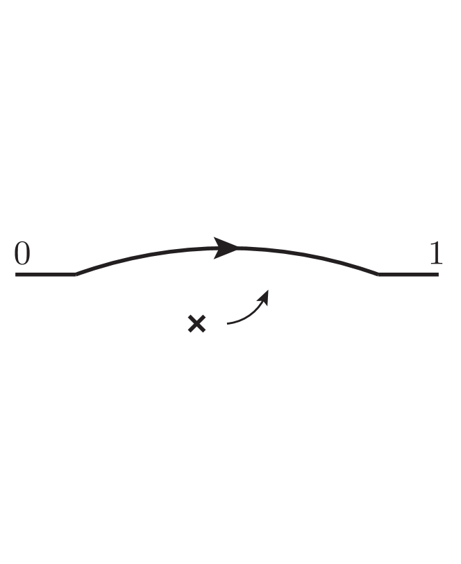
  (a)

  

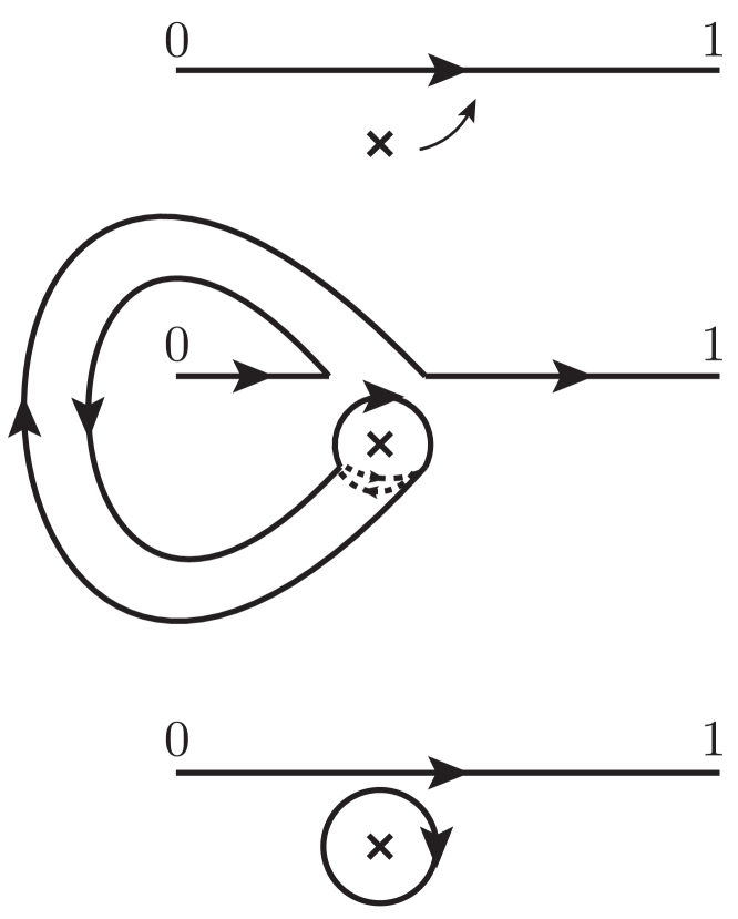
  (b)

  

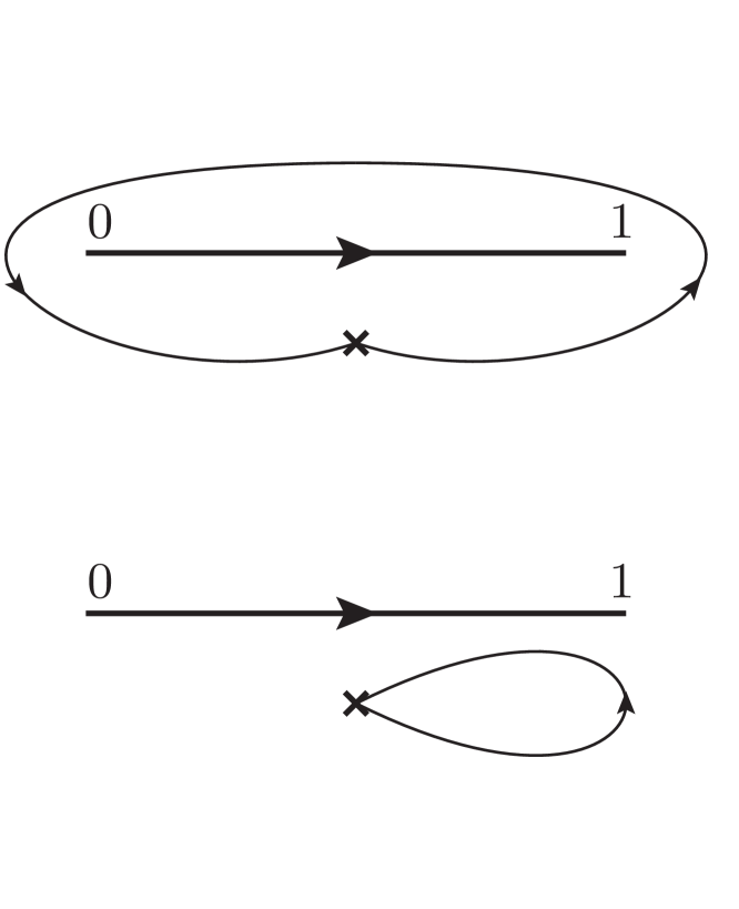
  (c)

  Figure 17: Contour deformations: a) Contour deformation to avoid an approaching pole. b) Deformation when the pole makes a complete circle around the end point. c) No contour deformation is required if the pole encircles both the end points.

  A simple example is the integral

  $$f_{1}(z)\,=\,\int_{0}^{1}\frac{d\omega}{\omega-z}\,.$$ (3.2)

  Here the integrand has a single pole in the $\omega$-plane at $\omega_{1}(z)=z$. We expect therefore singularities at $z=0$ and at $z=1$, while, if $z$ approaches the real axis in the region $0<z<1$, we can deform the contour to avoid the approaching pole, as in Fig. 17(a). It is also easy to predict that the singularities will be branch points: indeed, if $z$ encircles the point $z=0$ and comes back to its original location, then the singular point $\omega_{1}(z)$ also makes a circle around the end point, but, in doing so, it drags the contour along with it, as shown in Fig. 17(b). This new contour can be written as a sum of two contours, one of which encloses the pole. Thus we see that a residue is picked up, and there is a discontinuity equal to $2\pi\textrm{i}$ times that residue. The same residue is picked up each time the endpoint is circled, giving rise to the same amount of discontinuity: this shows that $z=0$ is a logarithmic branch point of $f(z)$, and the same of course holds true for the other end point, $z=1$. If, on the other hand, $z$ moves in such a manner that the pole never crosses the contour, then no residue is picked up: two such trajectories are shown in the Fig. 17(c); in both these cases we remain on the same branch of $f(z)$. All the above observations are obviously verified by the explicit result of integration which gives

  $$f_{1}(z)\,=\,\log\,\frac{z-1}{z}\,.$$ (3.3)

• Pinch singularity. A function $f(z)$ is singular at a point $z_{0}$ if two (or more) singularities of the integrand, say $\omega_{1}(z)$ and $\omega_{2}(z)$, approach the contour from opposite directions and eventually meet at the point $z_{0}$ preventing contour deformation. An example with a slight twist is given by

  $$f_{2}(z)\,=\,\int_{0}^{1}\frac{d\omega}{(\omega-z)(\omega-a)}\,,$$ (3.4)

  where we can take $1<a<2$ for the sake of the present argument. Here the integrand has two poles, $\omega_{1}(z)=z$ and $\omega_{2}(z)=a$. We already know that the presence of $w_{1}$ will lead to branch points in $f_{2}(z)$, at $z=0$ and at $z=1$, as in the previous example. The role of $\omega_{2}$, which is independent of $z$, is less obvious. To clarify it, take a point $z$, away from the contour, and lying on the principal sheet defined by the two branch points. The function $f(z)$ is analytic at this point, since both singular points $\omega_{1}$ and $\omega_{2}$ are away from the contour. Now, recall that if we make a closed circuit around an end point, say $z=1$, this will bring us to the second Riemann sheet. There is a new singularity present on this sheet, which is absent on the principal sheet: if for example one takes the point $z=a$ on the principal sheet and circles it around $z=1$, as shown in Fig. 18, in the process the contour gets dragged along, and it finally gets pinched with the pole at $w=a$ on the second sheet. By the same argument, it is clear that all other sheets (except the principal sheet) will have a singularity at $z=1+(a-1){\rm e}^{2\pi{\rm i}k}$, where $k$ is a non-vanishing integer.

  

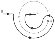
  Figure 18: The countour gets pinched on the second sheet producing a singularity of the function at $z=2$.

  As expected, these observations are verified by the explicit result of integration, which gives

  $$f_{2}(z)\,=\,\frac{1}{z-a}\,\ln\frac{a(z-1)}{z(a-1)}\,,$$ (3.5)

  where the pole at $z=a$ on the principal sheet is regulated by the vanishing logarithmic factor, while in all other sheets the pole survives, as the logarithm provides a non-vanishing $2\pi\textrm{i}k$ factor. Note that the pinch singularity examined here happens to involve a continuation to the second Riemann sheet, but of course pinches can arise on the principal sheet as well. It is easy to write the general form of a necessary condition for a pinch singularity to occur: if the integrand is a rational function (as is the case for Feynman integrals), the potential singularities will be located at the solutions of a polynomial equation of the form

  $$D\left(w,\left\{z_{i}\right\}\right)\,=\,0\,,$$ (3.6)

  where $D(w,\{z_{i}\})$ is the denominator of the integrand function, which can depend on several ‘external’ complex variables $z_{i}$. The condition for two roots of Eq. (3.6) to collide, on the surface defined by Eq. (3.6), is then simply

  $$\frac{\partial D}{\partial\omega}\,=\,0\,,$$ (3.7)

  as one readily verifies in the example in Eq. (3.4). Clearly, Eq. (3.7), together with Eq. (3.6), are only necessary conditions, since the two roots can for example collide away from the contour, or approach the contour from the same side, and furthermore a possible singularity may be cancelled by numerator factors.

• Pinch at infinity. Consider now the integral

  $$f_{3}(z)\,=\,\int_{1}^{a}\frac{d\omega}{1+z\omega}\,.$$ (3.8)

  The integrand has a pole at $\omega_{1}(z)=-1/z$, which gives end-point singularities at $z=-1/a$ and $z=-1$. The fact that the integrand decreases only as $w^{-1}$ for large $w$ does not seem to be relevant at first sight, since the integration contour is finite. In order to see the issue it is best to change variable to $y=1/\omega$, which gives

  $$f_{3}(z)\,=\,\int_{1/a}^{1}\,\frac{dy}{y\,(y+z)}\,.$$ (3.9)

  This displays the same branch points as Eq. (3.8), but it is now also clear that we are in a situation similar to our previous example: if one takes a point $z$ away from the contour, and circles one of the branch points, one can then approach the pole at $y=0$ and generate a pinch singularity, which will again be present on every Riemann sheet except the principal one. Indeed the integral gives

  $$f_{3}(z)\,=\,\frac{1}{z}\ln\frac{1+az}{1+z}\,.$$ (3.10)

These simple considerations can be extended to the case of several complex variables, though in full generality the mathematics becomes intricate (for a brief introductory discussion, and relevant references, see [265]). Fortunately, the search for infrared divergences in Feynman diagrams only requires simple tools, as we will see below.

3.1.2 The case of Feynman diagrams: the Landau equations

We now use the simple tools described in Section 3.1.1 to explore the singularities of a generic $L$-loop Feynman diagram with $M$ external lines carrying momenta $p_{i}$, $i=1,\ldots,M$. Let $G_{M}(p_{i})$ denote the corresponding Feynman integral, which is an integral over loop momenta that we denote by $k_{\ell}$, $\ell=1,\ldots,L$. We take the diagram to have $N$ internal lines, whose momenta we label by $q_{j}$, $j=1,\ldots,N$, and we represent the integral introducing Feynman parameters $\alpha_{j}$ for each internal line. We can then write

$$G_{M}(p_{i})\,=\,\int_{0}^{1}\prod_{j=1}^{N}d\alpha_{j}\;\delta\bigg{(}\sum_{i=1}^{N}\alpha_{i}-1\bigg{)}\int\prod_{\ell=1}^{L}\frac{d^{d}k_{\ell}}{(2\pi)^{d}}\,\frac{{\cal N}\left(\alpha_{j},k_{\ell},p_{i}\right)}{\Big{[}{\cal D}\left(\alpha_{j},k_{\ell},p_{i}\right)\Big{]}^{N}}\;,$$ (3.11)

where the numerator ${\cal N}$ contains coupling and spin dependence, and does not affect our search for potential singularities. A first necessary condition for the existence of a singularity is that the denominator should vanish,

$${\cal D}\big{(}\alpha_{j},k_{\ell},p_{i}\big{)}\,\equiv\,\sum_{j=1}^{N}\alpha_{j}\big{(}q_{j}^{2}-m_{j}^{2}\big{)}+{\rm i}\eta\,=\,0\;,$$ (3.12)

where the internal momenta $q_{j}$ are linear functions of external and loop momenta,

$$q_{j}\,=\,\sum_{r=1}^{L}\eta_{jr}\,k_{r}+\sum_{m=1}^{M}\beta_{jm}\,p_{m}\,.$$ (3.13)

For any consistent assignment of loop momenta to the graph edges, the incidence matrices $\eta_{jr}$ and $\beta_{jm}$ have entries in the set $\{-1,0,1\}$: for example, $\eta_{jr}=0$ if loop momentum $k_{r}$ does not flow through line $j$, while $\eta_{jr}=1$ if the loop momentum $k_{r}$ flows through the $j$th line in the same direction as $q_{j}$, and $\eta_{jr}=-1$ in the opposite case.

There are a total of $dL+N-1$ independent integration variables in Eq. (3.11), each one integrated along a path that can be modified, if required, to provide analytic continuation. A necessary condition for the existence of a singularity is therefore that all integration variables be localised either at a pinch surface or at an endpoint: if any variable is not constrained, the direction of that variable in the multi-dimensional complex integration space can be used to deform the contours. At least for non-exceptional configurations of the external momenta, since the denominator is a sum of propagator denominators with positive coefficients, the condition ${\cal D}(\alpha_{j},k_{\ell},p_{i})=0$ is realised when, for each internal line $j$, either the corresponding momentum $q_{j}$ is on the mass-shell, or the corresponding Feynman parameter $\alpha_{j}$ vanishes. That is,

$${\rm either}\qquad q_{j}^{2}-m_{j}^{2} = 0\,,$$ (3.14a)

$${\rm or}\hskip 56.9055pt\alpha_{j} = 0\,.$$ (3.14b)

Next, we need to make sure that all variables are localised either at end-point or at pinch singularities. Here the important point about the graph representation in Eq. (3.11) is that the denominator ${\cal D}$ is quadratic in the loop momenta $k_{\ell}$, and linear in the Feynman parameters $\alpha_{j}$. This leads immediately to the following conclusions.

• Since ${\cal D}(\alpha_{j},k_{\ell},p_{i})$ is linear in $\alpha_{j}$, there can only be a single pole in the $\alpha_{j}$ plane, so the only possible singularities are end-point singularities at $\alpha_{j}=0$ or at $\alpha_{j}=1$. On the other hand, if any of the $\alpha_{j}=1$, then all the other $\alpha_{k}$ must vanish simultaneously because of the $\delta$ function in Eq. (3.11), a configuration which is not relevant for infrared divergences.

• Pinch singularities, on the other hand, do arise for loop momentum components, since Eq. (3.12) is quadratic in $k_{j}^{\mu}$. The condition for the two poles in the $k_{j}^{\mu}$ complex plane to coalesce is given by Eq. (3.7), which we rewrite here as

  $$\frac{\partial}{\partial k_{j}^{\mu}}\,{\cal D}(\alpha_{j},k_{\ell},p_{i})\,=\,0\;.$$ (3.15)

  Upon substituting Eq. (3.12) and Eq. (3.13), Eq. (3.15) gives

  $$\displaystyle{\sum\limits_{i\,\in\,\textrm{loop}\,j}}\eta_{ij}\,\alpha_{i}q_{i}\,=\,0\,,\quad\textrm{for each}\,\,j\,,$$ (3.16)

  where the sum includes all the lines $i$ through which loop momentum $k_{j}$ runs.

• Finally, we note that the integration domain of loop momentum components extends to infinity, and one should also consider end-point singularities for these integrals. The corresponding singularities, however, are ultraviolet, and we are assuming that they have already been taken care of by the inclusion of appropriate renormalisation counterterms.

Eqs. 3.12 and 3.15 or, equivalently, Eq. (3.14) and Eq. (3.16), are known as Landau equations [270]. The first set of Landau equations, setting ${\cal D}(\alpha_{j},k_{\ell},p_{i})=0$, defines a set of surfaces in the $(dL+N-1)$-dimensional space of integration variables. The surfaces on which the second set of equations are also satisfied are called pinch surfaces. On such surfaces, all internal lines may be on the mass shell ($\alpha_{i}\neq 0,\forall\,i$), or some of the lines may be off the mass shell, provided the corresponding $\alpha_{i}=0$. Lines with a vanishing Feynman parameter do not appear in the second set of Landau equations: as a consequence, since these lines are irrelevant for the conditions determining a pinch, when studying the corresponding pinch surfaces we can graphically reduce the lines to points. This procedure gives us a new set of diagrams, specific to the pinch surface under consideration, which are called reduced diagrams.

In this context, let’s make here a simple observation that will be useful later [165]. If we single out a massless line $l$ in loop $j$, which carries momentum $q_{l}$, and the corresponding Feynman parameter is $\alpha_{l}$, then the second set of Landau equations for loop $j$ becomes

$$\alpha_{l}q_{l}\,+\,\displaystyle{\sum\limits_{i\,\in\,\textrm{loop}\,j,\,i\neq l}}\alpha_{i}q_{i}\,=\,0\,,$$ (3.17)

where we chose the line momenta $q_{i}$ to flow in the same direction as the loop momentum $k_{j}$. If line $l$ is massless, and if $q_{l}^{\mu}=0$ (so that $l$ is on shell), we see that this line drops out of the Landau equation, leaving no trace, as it is not even required for momentum conservation. This means that, once the integral is trapped on a pinch surface, adding an arbitrary number of soft massless lines does not alter the requirements on the other lines of the graph, in order for the integral to remain localised on the pinch surface.

3.1.3 The Coleman-Norton physical picture

The Landau equations provide, in principle, a solution to the problem of locating all potential singularities of Feynman integrals. The actual task, however, remains daunting, especially if one is attempting to work to all orders in perturbation theory: without any further information, it still appears that Feynman diagrams need to be treated one by one, and each one will present a plethora of pinch surfaces. As it turns out, the search for solutions of the Landau equations for external momenta in the physical region is greatly simplified by a remarkably simple and intuitive criterion introduced by Coleman and Norton (CN) in Ref. [271]. As we will see below, the CN criterion allows to quickly grasp the structure of solutions of the Landau equation for infinite classes of Feynman diagrams, paving the way for studies to all orders in perturbation theory.

The CN criterion for the existence of a solution of the Landau equations for physical values of the external momenta can be stated as follows: a candidate pinch surface of a given Feynman integral provides a solution to the Landau equations if and only if the corresponding reduced Feynman graph can be interpreted as describing a classical scattering processes involving on-shell particles carrying the momenta assigned to each line of the reduced graph.

To be more precise, let us consider a generic pinch surface and the corresponding reduced diagram. Note that we have already localised the Feynman parameters of off-shell lines by setting them to zero. It is now necessary to pinch the contour of every loop momentum component on the configuration where all surviving lines are on-shell: in this way, non-vanishing Feynman parameters cannot be used to escape the pinch surface, since they multiply vanishing factors given by on-shell propagator denominators. Consider now a line carrying momentum $q$, and let $\alpha$ be the Feynman parameter for that line. As the contour for every loop-momentum component $k_{\ell}^{\mu}$ is pinched and forced to be on the real axis, we see from Eq. (3.13) that $q$ will take real values for physical external momenta $p_{j}$. Since $q$ is on-shell, $q^{2}=m^{2}$, we can write $q^{\mu}=m\,dx^{\mu}/d\tau$, where $\tau$ is the proper time and $x^{\mu}(\tau)$ parametrises the classical trajectory of a free particle with momentum $q$, which of course moves on a straight line with constant four-velocity. We can rearrange this into

$$\Delta x^{\mu}\,=\,\frac{\Delta\tau}{m}\,q^{\mu}\,.$$ (3.18)

If we now make the identification

$$\frac{\Delta\tau}{m}\,\equiv\,\alpha\,,$$ (3.19)

then the product $\alpha q^{\mu}$ can be interpreted as the space-time displacement of a classical particle of mass $m$ in the proper time $\Delta\tau=m\alpha$. Considering the Lorentz invariant ratio

$$\frac{\Delta t}{q^{0}}\,=\,\frac{\Delta\tau}{m}\,,$$ (3.20)

we can also say that the time of propagation is equal to $\alpha q^{0}$ in the reference frame in which the particle has energy $q^{0}$. This shows that the space-time picture we are constructing is not limited to massive particles: for a massless particle, we can pick a frame in which the energy carried by the line has a given value $q^{0}$, and we can replace Eq. (3.18) with $\Delta x^{\mu}\,=\,\Delta t\,\beta^{\mu}$, where $\beta^{\mu}$ is the light-like four-velocity associated with the momentum $q^{\mu}$, $\beta^{\mu}=\{1,{\bf q}/q^{0}\}$. The Feynman parameter can now be identified with the l.h.s of Eq. (3.20). Note that Feynman parameters are positive on the undeformed contours, which is consistent with particles moving forward in time.

Within this framework, it is tempting to interpret the two endpoints of each line as space-time points separated by a distance $\alpha q^{\mu}$. For this interpretation to be consistent, however, the separation between any two vertices in the reduced diagram should be independent of the path taken to join them. Equivalently, if we start at a vertex, make a closed loop, and arrive back at the same vertex, the total displacement should be zero. It is easy to verify that the second Landau equation, Eq. (3.16), precisely guarantees that this is the case. This gives us the Coleman-Norton physical picture: the leading singularities of reduced diagrams in the physical region are supported on configurations where the internal lines can be regarded as the paths of classical particles moving freely between the vertices, while internal vertices can be regarded as points of interactions, where particle velocities change.

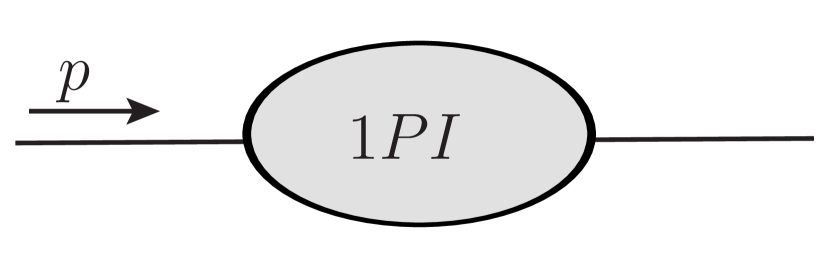
(a)

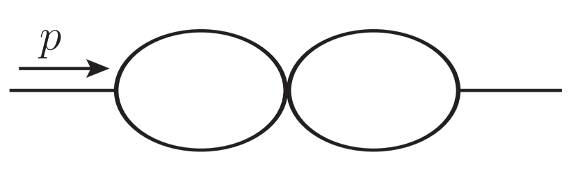
(b)

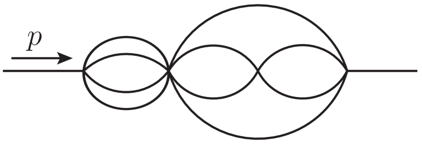
(c)

Figure 19: (a)1PI contributions to a two-point function, (b) A two-loop reduced diagram exhibiting a threshold at $p^{2}=4m^{2}$, (c) A seven-loop reduced diagram with a threshold at $p^{2}=16m^{2}$.

The intuitive power of the CN picture can hardly be overstated: it turns a rather abstract mathematical problem into a question about classical scattering, and very general results for entire classes of Feynman diagrams can readily be derived. To provide a simple, yet powerful example [2], consider the two-point correlator for a theory with only one species of particles with mass $m$. In the leftmost panel of Fig. 19, the shaded ellipse represents the one-particle-irreducible (1PI) contributions to the correlator in this theory, assuming the external momentum to be $p$. Following the CN picture, we must now seek classical processes in which a source carrying (off-shell) momentum $p$ can split into a set of on-shell particles, which later reassemble into a single one. Clearly, any splitting producing particles with non-vanishing momenta in directions transverse to $p$ is not allowed, since, by momentum conservation, such particles would propagate in opposite directions, and could never meet again. This leaves us with the possibility of collinear splittings, however two on-shell lines with three-momenta ${\bf k}_{1}$ and ${\bf k}_{2}$ cannot in general merge to produce an on-shell line with three-momentum ${\bf k}={\bf k}_{1}+{\bf k}_{2}$, as the invariant mass of that line would be greater than $m$. Only one set of possibilities is left: for $p^{2}=n^{2}m^{2}>0$, with integer $n$, a simple CN process is easily identified in the rest frame of $p$: the off-shell source particle can split into $n$ on-shell particles at rest, and these can further merge and split any number of times, provided particle number is conserved; finally, they can merge again to reconstruct the momentum $p$. With remarkable generality, we can conclude that the only possible singularities of two-point functions of massive particles are located at the thresholds for the creation of $n$ on-shell particles, which are called normal thresholds, and are clearly and directly related to unitarity cuts. Thus, a single analysis has solved the problem for an infinite set of Feynman diagrams, regardless of the specific details of the interactions of the massive particles involved: Fig. 19(b) and Fig. 19(c) show two examples of reduced diagrams for $p^{2}$ equal to $4m^{2}$ and $16m^{2}$ respectively.

Note that the argument can be rephrased in a boosted frame where $p$ is not at rest, shedding light on the values of Feynman parameters allowed by the CN constraints. Imagine one creates two particles of equal masses which then move together collinearly. If they have different energies, we can move to a frame where the one with the smaller momentum will be at the rest. Now the two particles can never meet again, unless the second particle scatters off a ‘wall’ to reverse its direction; this circumstance can be realised only if we include an extra vertex, which is a situation we will encounter when we discuss three-point graphs. Thus, the two massive particles can meet at a later time without encountering a new vertex only if they have equal energies. In general, the CN time they take to merge is given by $\Delta t=\alpha_{1}E_{1}=\alpha_{2}E_{2}$, therefore the Feynman parameters are constrained to satisfy $\alpha_{1}=\alpha_{2}$. The same physical picture for $n$ massive particles gives equal values for all $\alpha_{i}$, and finally the presence of the factor $\delta(1-\sum_{i}\alpha_{i})$ enforces

$$\alpha_{1}\,=\,\alpha_{2}\,\ldots\,=\,\alpha_{n}\,=\,1/n\,.$$ (3.21)

Clearly, this simple analysis of two-point functions can be extended to higher-point functions as well, allowing the identification of at least some of their potential singularities. As an example, one can consider a four-point function in the $s$-channel physical region. When the two incoming momenta have a total invariant mass $s=n^{2}m^{2}$, with $n$ integer, in their center-of-mass frame one finds that the same CN process that was identified for the two-point function is available also in this case: there is just enough energy to create $n$ on-shell particles at rest, and these particles can interact conserving particle number until they finally decay into the final state pair. Note also that the discussion of two-point functions for massive particles has implications for the massless case: if the off-shell source carrying momentum $p$ couples only to massless particles, then all the normal thresholds collapse to the point $p^{2}=0$. One must however remember, as discussed at the end of Section 3.1.2, that adding a soft particle with a vanishing momentum $q$ does not influence the Landau equations: in the CN picture, soft lines correspond to vanishing displacements $\Delta x^{\mu}$ and do not modify the classical scattering configuration. Two-point functions involving massless particles will therefore potentially be affected by soft singularities, and power counting techniques will need to be employed to check if these lead to actual divergences.

In order to prepare the ground for our analysis of massless form factors in Section 4, we need to consider in more detail the case of three-point functions. First of all, let us note that the general structure of singularities becomes significantly more complicated when $n>2$ external particles are involved, since the resulting Feynman integrals are functions of several complex variables: for example, a three-point function in a theory with only one species of particles with mass $m$ will depend on three dimensionless ratios, say $x=p_{1}^{2}/m^{2}$, $y=p_{2}^{2}/m^{2}$, and $z=p_{3}^{2}/m^{2}$, with $p_{3}^{2}=(p_{1}+p_{2})^{2}$.

One can readily verify that the presence of a third particle (and therefore of at least one more interaction vertex, as compared to the two-point function) allows for singularities which are not related to normal thresholds, and are usually referred to as anomalous thresholds. While unitarity cuts arise by putting on the mass shell exactly the number of lines needed to split a given diagram into two disconnected subdiagrams, containing respectively initial-state and final-state particles, anomalous thresholds arise from configuration in which a larger number of lines are on-shell, and the diagram may split into several disconnected pieces (thus they are often referred to as generalised unitarity cuts, while the configuration in which all internal lines are on-shell is often described as leading singularity). To illustrate this, consider the simple case of a one-loop triangle diagram, depicted in Fig. 20, which of course can be understood as a reduced diagram arising from a more complicated configuration. It is not difficult to find a CN process such that the three (massive) lines be on shell: one may for example envisage two particles being created with momenta $k_{1}$ and $k_{2}$ at vertex $A$. If the source momentum $p=k_{1}+k_{2}$ is timelike, $p^{2}>0$, one can consider the frame in which $p$ is at rest, so that the two produced particles are emitted back to back. Without further scattering, they could never meet again at any later time at vertex $C$. One can however envisage one of the two particles bouncing off a ‘wall’ at vertex $B$: if sufficient momentum is injected there, the particle can reverse its direction to annihilate the other one at vertex $C$. Clearly, the existence and location of this singularity will depend upon the values of the external invariants $x$, $y$ and $z$: in particular, the singularity may or may not appear on the physical Riemann sheet.

As was the case for two-point functions, the massless limit introduces new pinch surfaces, which are the ones of interest for the analysis of infrared divergences. In particular, given an existing configuration with on-shell lines, one is always free to add soft massless lines, without affecting the Landau equations. Furthermore, as discussed already in Section 1, a massless line can split into two or more collinear massless lines, while conserving four-momentum and keeping all lines on the mass shell. We illustrate these facts in some more detail in Section 3.1.4 below.

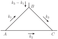
Figure 20: Momentum routing for a three-point graph displaying possible anomalous thresholds, as discussed in the text.

3.1.4 Pinch surfaces of massless vertex graphs

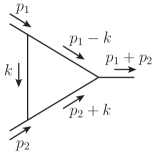
Figure 21: One-loop vertex correction to the three-point function in a massive scalar theory.

To illustrate the situation for massless three-point functions, consider the simple one-loop triangle graph depicted in Fig. 21. We consider a scalar graph, since for our present considerations the numerator structure is not relevant. The expression for the graph after Feynman parametrisation is of the form of Eq. (3.11), and can be written as

$$G_{3}(p_{1},p_{2})\,=\,\int_{0}^{1}\prod_{j=1}^{3}d\alpha_{j}\int\frac{d^{d}k}{(2\pi)^{d}}\,\frac{\delta\big{(}\sum_{i=1}^{3}\alpha_{i}-1\big{)}}{\Big{[}\alpha_{1}k^{2}+\alpha_{2}(p_{1}-k)^{2}+\alpha_{3}(p_{2}+k)^{2}+{\rm i}\eta\Big{]}^{3}}\;,$$ (3.22)

where we take $p_{1}^{2}=p_{2}^{2}=0$. The second Landau equation for this graph reads

$$\alpha_{1}k^{\mu}-\alpha_{2}\big{(}p_{1}-k\big{)}^{\mu}+\alpha_{3}\big{(}p_{2}+k\big{)}^{\mu}\,=\,0\,,$$ (3.23)

and we need to pick solutions such that, if a given $\alpha_{i}$ is not vanishing, then the corresponding four-momentum must be on shell. Setting for the moment aside ordinary and anomalous thresholds, we see that two new sets of pinch surfaces arise in the massless case.

• Collinear pinch surfaces. If, for example, $k^{\mu}$ is parallel to $p_{1}^{\mu}$, so that $k^{\mu}=x\,p_{1}^{\mu}$, we see that the line carrying momentum $p_{1}-k$ is on shell, while the line $p_{2}+k$ is off shell for generic configurations of external momenta. We can thus find a solution of the Landau equations by setting $\alpha_{3}=0$ and then requiring that

  $$x\alpha_{1}\,=\,(1-x)\alpha_{2}\,,$$ (3.24)

  in order to solve Eq. (3.23). The reduced diagram for this pinch surface is shown in Fig. 22(b), left panel. The corresponding CN configuration has two light-like particles starting from the origin at $t=0$ and moving in the direction of $p_{1}^{\mu}$ with different energies, $x\,p_{1}^{0}$ and $(1-x)p_{1}^{0}$ respectively; they meet again when their CN displacements become equal, which happens when Eq. (3.24) is satisfied, see the second diagram in Fig. 22(b). Note that CN times are positive when $0<x<1$, so that the singular configuration can be on the integration contour and thus on the physical Riemann sheet. Needless to say, an identical situation is reproduced when the loop momentum is collinear to $p_{2}$, say $k^{\mu}=-y\,p_{2}$. Then the line carrying momentum $p_{1}-k$ will be off-shell, and the Landau equations can be solved by setting $\alpha_{2}=0$ and then requiring that

  $$y\alpha_{1}\,=\,(1-y)\alpha_{3}\,.$$ (3.25)

• Soft pinch surfaces. As discussed in Section 3.1.2, in a massless theory one can always build solutions of the Landau equations by adding particles with vanishing momenta, which do not affect the equations, nor the relevant CN configurations. In the present case, one can for example solve Eq. (3.23) by picking any $\alpha_{1}\neq 0$ and setting

  $$k^{\mu}\,=\,0\,,\qquad\alpha_{2}\,=\,\alpha_{3}\,=\,0\,.$$ (3.26)

  In this limit, all particles circulating in the loop are on-shell, so that the reduced diagram coincides with the original one, as depicted in Fig. 22(a); the soft particle carrying momentum $k$ does not contribute to the CN displacement sum, Eq. (3.16), corresponding to the fact that a particle with vanishing four-momentum is fully delocalised. Note that, while the diagram we are considering is not symmetric under the exchange of the external particles, since $(p_{1}+p_{2})^{2}\neq 0$, there are nevertheless soft pinch surfaces associated with the soft limit for any particle circulating in the loop: these are most easily detected by changing the parametrisation of the loop momenta, but even with our current choice we see that one can solve Eq. (3.23), for example, by taking $k^{\mu}=p_{1}^{\mu}$ and $\alpha_{1}=\alpha_{3}=0$. Note also that all our discussion so far does not depend on particle spins, nor on the specifics of their interactions: the one-loop triangle diagram can arise as a reduced diagram in any theory, even if the interactions are not cubic in the fields. In order to ascertain if the pinch surfaces we have identified give actual divergences, we will need the power-counting tools discussed in Section 3.2.

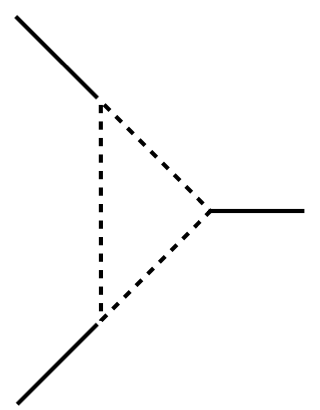
(a)

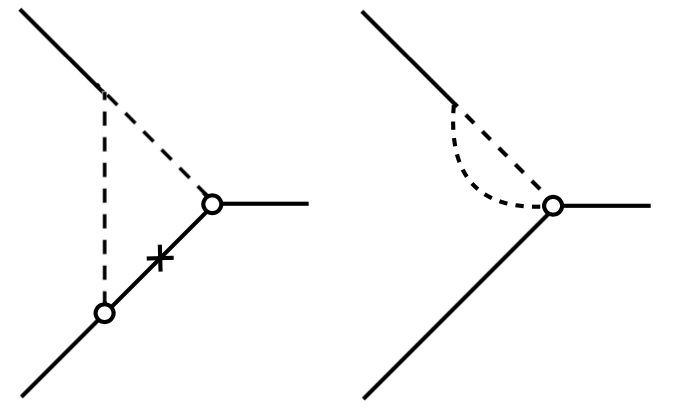
(b)

Figure 22: (a) Reduced diagram for the soft pinch surface. (b) Building the reduced diagram for a collinear pinch surface. In the left panel of (b) we highlighted with a cross the off-shell propagator that shrinks to a point, yielding the right panel. Dashed lines mark on-shell propagators.

It should be clear from the above discussion of the one-loop scalar diagram that we have actually identified sets of pinch surfaces for an infinite set of Feynman diagrams, to any perturbative order. For example, adding further loops involving soft particles will automatically solve the Landau equations. Similarly, adding more particles collinear to either $p_{1}$ or $p_{2}$ will provide new pinch surfaces, since each new particle will add a Feynman parameter, and a single constraint of the form of Eq. (3.24), so that the resulting system of equations will remain solvable. In the CN picture, if two particles are produced back to back at the hard interaction vertex, they can never meet again, however each particle can split into collinear multiplets which then recombine at later times, and these two jets of particles evolving in opposite directions can always be connected by means of soft radiation. We are thus beginning to develop a general picture of the singularity structure of massless form factors to all orders: in a generic diagram, the hard interaction can be dressed with any number of off-shell virtual corrections, which shrink to a point in the corresponding reduced diagram; infrared singularities may arise when, out of this hard effective vertex, two jets of collinear particles emerge, which in turn can be connected to each other by a soft subdiagram, where all particles have vanishing four-momentum. This is a very significant simplification of the generic situation we started with, but we will see in what follows that the final form of the factorisation we are seeking is simpler still.

3.2 Identifying actual singularities: infrared power counting

Up to this point, we have presented a set of conditions to identify all the potential sources of singularities in Feynman integrals, in particular infrared divergences. The derivation requires that the poles of the integrand must be forced to lie on the integration contour. Clearly, this is only a necessary condition for actual divergences to occur: first of all, the detected singularity might be - for example - a branch cut and not a divergence; next, positive powers of the integration variables can appear in the numerator of the integrand and mitigate the potential divergence. Sufficient conditions to identify the kinematic configurations that result in IR singularities can only be derived from power-counting techniques, reminiscent of those employed in the UV to study renormalisation.

In the UV case, power counting is straightforward, since the singular region is approached when all loop momentum components become very large. One may thus detect the behaviour of the integral by rescaling loop momenta as $k^{\mu}\to\Lambda\bar{k}^{\mu}$, and counting powers of $\Lambda$. Since a Feynman integrand is a product of rational factors, one may expand each factor in powers of $\Lambda$, retaining only the leading power in each factor: the resulting overall power of $\Lambda$ gives the superficial degree of UV divergence of the diagram under study. The situation in the infrared is more intricate: as we have seen, potential singularities arise in the massless limit when loop momenta become soft or collinear to some of the external momenta. Different loop-momentum components must then be treated differently, as only some of them are related to singularities of the integral. It is not difficult to make this analysis systematic, as we discuss below.

3.2.1 Intrinsic and normal coordinates, and homogenous integrals

To study infrared power counting, it is best to revert to momentum-space integrals, before the introduction of Feynman parameters (see, however, Ref. [224] for a coordinate space representation). In full generality, a $p$-dimensional pinch surface $\Sigma_{p}$ in the $D$-dimensional loop momentum space ${\cal L}$ (where $D=dL$ for an $L$-loop diagram in $d$ space-time dimensions) will be characterised by $D-p$ conditions, which can be cast in the form

$$F_{i}\left(k_{\ell}^{\mu}\right)\,=\,0\qquad i\,=1,\ldots,D-p;\quad\ell\,=\,1,\ldots,L\,.$$ (3.27)

For our purposes, the constraints $F_{i}$ will be linear, and the resulting surfaces will be hyperplanes; the discussion can however be generalised to non-linear constraints and curved surfaces. Given any differentiable set of constraints $F_{i}$, one can pick a parametrisation of ${\cal L}$ such that $p$ coordinates $k_{I}$ parametrise the surface $\Sigma_{p}$, while the remaining $D-p$ coordinates $k_{N}$ serve to measure the distance of any point in ${\cal L}$ from $\Sigma_{p}$. Changing the values of the coordinates $k_{I}$ moves a point within the surface, so these coordinates are called intrinsic; changing the value of the coordinates $k_{N}$ moves points away from the pinch surface, and these coordinates are correspondingly called normal. The strength of the singularity encountered on $\Sigma_{p}$ is controlled by the behavior of the integrand as a function of normal coordinates, and one is free to define normal coordinates such that their zeros lie on the pinch surface $\Sigma_{p}$.

Since we are interested in the behaviour of the reduced graph near the surface $\Sigma_{p}$, we can again take advantage of the structure of the Feynman integrand, which is a product of rational factors, and we can expand each factor in the denominator and in the numerator in powers of the normal coordinates, retaining the lowest order approximation. Thus, given a reduced graph $G$, and for every pinch surface $\Sigma$ of $G$, we can write

$$G_{\Sigma}(p_{i})\,=\,\int d^{p}k_{I}\,d^{D-p}k_{N}\;{\cal I}\big{(}p_{i},k_{I},k_{N}\big{)}\,,$$ (3.28)

where $p_{i}$ denotes the external momenta. We then associate with $G_{\Sigma}$ a homogenous integral

$$\overline{G}_{\Sigma}\,=\,\int d^{p}k_{I}\,d^{D-p}k_{N}\;\overline{\cal I}\big{(}p_{i},k_{I},k_{N}\big{)}\,,$$ (3.29)

where $\overline{\cal I}$ is the leading-power approximation of ${\cal I}$ with respect to the set of normal coordinates.

Moving internal lines away from the mass shell will take the graph off the pinch surface. Virtualities of internal lines will therefore be proportional to normal coordinates, and the ratio of these virtualities to the hard scale $Q$ will determine how close or how far we are from the surface. In the next section, we will present the analysis of two simple one-loop examples, using again a three-point graph as a laboratory, and then we will proceed by illustrating how the one-loop results generalise to all perturbative orders.

3.2.2 One-loop examples: the QED vertex graph

Let us consider the one-loop QED vertex graph, adapting what we have already presented in Section 1.1 and for the scalar theory in Section 3.1.4. In the massless limit, we can pick a frame in which the external momenta in are given by

$$q = (Q,0,0,0)\,,$$

$$p_{1} = \big{(}Q/2,0,0,Q/2\big{)}\,,$$ (3.30)

$$p_{2} = \big{(}Q/2,0,0,-Q/2\big{)}\;,$$

where $Q$ is the photon virtuality, giving the hard scale of the problem. The expression of the graph (see also Eq. (1.10)) is

$$G_{3}(p_{1},p_{2})\,=\,{\rm i}e^{2}\mu^{2\epsilon}\,\int\frac{d^{d}k}{(2\pi)^{d}}\,\frac{\mathcal{N}(p_{1},p_{2},k)}{(k^{2}+{\rm i}\eta)\big{[}(p_{1}-k)^{2}+{\rm i}\eta\big{]}\big{[}(p_{2}+k)^{2}+{\rm i}\eta\big{]}}\,,$$ (3.31)

where ${\cal N}(p_{1},p_{2},k)$ contains spinors and Lorentz structures. We already know from the Landau equation analysis in Section 3.1.4 that this graph has pinch surfaces for configurations where the loop momentum $k$ is soft, and/or collinear to either fermion line. Let us now consider each case in turn.

Near the soft pinch surface, $k^{\mu}\to 0$, all the components of the virtual photon momentum $k$ are normal coordinates, and there are no intrinsic coordinates. Upon approximating the factors in the denominator by their lowest order expressions in the expansion in powers of $k^{\mu}$, we readily recognise, unsurprisingly, that the homogenous integral is given by the eikonal approximation, as in Eq. (1.11) and Eq. (2.39),

$$\overline{G}_{3,\,{\rm soft}}(p_{1},p_{2})\,=\,{\rm i}e^{2}\mu^{2\epsilon}\int\frac{d^{d}k}{(2\pi)^{d}}\,\frac{{\cal N}(p_{1},p_{2},0)}{(k^{2}+{\rm i}\eta)(2p_{2}\cdot k+{\rm i}\eta)(-2p_{1}\cdot k+{\rm i}\eta)}\,.$$ (3.32)

In the present case, it is easy to see directly that the soft homogeneus integral is dimensionless and logarithmically divergent in $d=4$. In a more general setting, in order to determine the distance from the soft pinch surface as a function of the normal coordinates, we can choose a scaling variable $\lambda_{\rm s}$, and impose the same scaling for each momentum component, as was done in the UV region, but this time taking the limit $\lambda_{\rm s}\to 0$. Thus we can set

$$k^{\mu}\,=\,\lambda_{\rm s}\bar{k}^{\mu}\,,$$ (3.33)

and count powers of $\lambda_{\rm s}$ in the homogeneous integral. The scaling variable $\lambda_{\rm s}$ is often taken to be dimensionless, however, in case one is interested in keeping track of powers of the hard scale $Q$, one can also take $\lambda_{\rm s}$ to have dimensions of energy, and treat the reduced components $\bar{k}^{\mu}$ as ‘angular’ variables [67]. In this case, one can choose, for example

$$\lambda_{\rm s}\,=\,\sum_{\mu}\big{|}k^{\mu}\big{|}\,,$$ (3.34)

so that the dimensionless variables $\bar{k}^{\mu}$ are normalised as

$$\sum_{\mu}\big{|}\bar{k}^{\mu}\big{|}\,=\,1\,.$$ (3.35)

Treating $\lambda_{\rm s}$ as a dimensionless parameter, substituting Eq. (3.33) in the soft homogeneous integral, Eq. (3.32), and replacing every factor of $p_{1}$ and $p_{2}$ by the hard scale $Q$, we verify that

$$\overline{G}_{3,\,{\rm soft}}(p_{1},p_{2})\,\sim\,\frac{1}{\lambda_{\rm s}^{4-d}}\frac{1}{Q^{2}}\times{\cal N}(p_{1},p_{2},0)\,.$$ (3.36)

In a gauge theory, as seen already in Eq. (1.10), the homogeneous numerator is proportional to $Q^{2}$, so, as announced, the integral is logarithmically divergent in $d=4$, and contributes at leading power in $Q$.

Turning now to the collinear limit, it is useful to introduce light-cone coordinates, such that any four-vector is expressed as $x^{\mu}=(x^{+},x^{-},\bf{x}_{\perp})$, with

$$x^{+}\,=\,\frac{x_{0}+x_{3}}{\sqrt{2}}\,,\qquad x^{-}\,=\,\frac{x_{0}-x_{3}}{\sqrt{2}}\,,$$ (3.37)

so that

$$x^{\mu}y_{\mu}\,=\,x^{+}y^{-}+x^{-}y^{+}-\bf{x}_{\perp}\cdot\bf{y}_{\perp}\,,$$ (3.38)

while the measure of integration becomes

$$d^{d}k\,=\,dk^{+}dk^{-}d^{d-2}k_{\perp}\,.$$ (3.39)

When the photon is collinear to the electron carrying momentum $p_{1}$, in the frame in which Eq. (3.2.2) applies, $k_{\perp}$ and $k^{-}$ must vanish, while we can set $k^{+}=zp_{1}^{+}$. Changing the value of $z$ leaves the loop momentum on-shell, so that configurations with any $z$ in principle belong to the collinear pinch surface: $z$ is an intrinsic coordinate; clearly, the azimuthal angle $\phi$ for the transverse momentum ${\bf k}_{\perp}$ is also an intrinsic coordinate. Note however that, using the CN physical picture, the graph can be interpreted as a classical collinear splitting of massless particles with on-shell momenta only if $0\leq z\leq 1$. If $z$ is outside this range, the photon propagator is still on shell, but the CN interpretation is not valid, and we expect that the contour may be deformed to avoid the singularity. Considering the remaining variables, we see that generic non-vanishing values of $k^{-}$ and $k_{\perp}$ will move the photon away from the mass shell: $k^{-}$ and $k_{\perp}$ are normal coordinates.

Expressing $G_{3}(p_{1},p_{2})$ in these variables, expanding each factor in powers of the normal variables, and retaining the leading power in each one of them, we find the collinear homogeneous integral

$$\overline{G}_{3,\,{\rm coll}_{1}}(p_{1},p_{2}) = \frac{{\rm i}e^{2}\mu^{2\epsilon}}{(2\pi)^{d}}\int dz\,\,\frac{{\cal N}(p_{1},p_{2},z)}{2p_{2}^{-}z+{\rm i}\eta}$$

$$\times\,\int dk^{-}d^{d-2}k_{\perp}\,\frac{1}{2k^{+}k^{-}-k_{\perp}^{2}+{\rm i}\eta}\,\frac{1}{-2(1-z)p_{1}^{+}k^{-}-k_{\perp}^{2}+{\rm i}\eta}\,,$$

where in the numerator we have set $k^{-}=k_{\perp}=0$, but retained the dependence on $k^{+}$. We see that the photon and electron denominators are linear in the normal coordinate $k^{-}$, but quadratic in $k_{\perp}$. The natural scaling choice, ensuring that these denominators are homogeneous in the scaling parameter, and linear in normal coordinates, is therefore to take

$$k^{-}\,=\lambda_{\rm c}\,\bar{k}^{-}\,,\qquad k_{\perp}^{2}\,=\,\lambda_{\rm c}\,{\bar{k}}_{\perp}^{2}\,,$$ (3.41)

where we choose $\lambda_{\rm c}$ to be dimensionless. We see that the collinear homogeneous integral is ${\cal O}(\lambda_{c}^{\epsilon})$, implying a logarithmic divergence in $d=4$. We also see that the off-shell positron line gives a $1/Q$ suppression, however the collinear numerator also grows linearly with $Q$, so that the collinear region contributes at leading power in $Q$, as was the case for the soft region. In the remainder of Section 3, we will omit the subscripts from the scaling parameters $\lambda_{\rm s}$ and $\lambda_{\rm c}$, with the understanding that soft and collinear scalings are defined by Eq. (3.33) and in Eq. (3.41).

Let us conclude this section with two important notes. First, recall that the soft and collinear regions overlap: this is reflected in the fact that the collinear homogeneous integral in Eq. (3.2.2) still has a soft singularity, as $z\to 0$, and similarly the soft homogeneous integral in Eq. (3.32) has collinear singularities when $k$ becomes parallel to either $p_{1}$ or $p_{2}$. At the moment, this is not a serious concern, as we are only interested in determining the strength of the singularities. At a later stage, when building an explicit factorised expression for amplitudes and cross sections, a careful treatment of overlapping singularities will become necessary. A second important caveat emerges from the observation that different components of loop momenta may become small at different rates, as is the case in the collinear region, Eq. (3.41). This raises the possibility that there could be different scalings of momentum components (for example combining soft and collinear limits with different strengths) that might need to be treated separately. We will briefly get back to this issue in Section 5: here we note that this is in principle a process-dependent question, that can only be addressed via a detailed diagrammatic analysis. The issue is particularly relevant when factorisation theorems are constructed by means of effective field theories, where the relevant momentum modes must be selected a priori. On the other hand, once a particular scaling has been understood to be relevant, the effective theory can be extended to include it (see, for example, Refs. [272, 273, 274]).

3.2.3 Soft and collinear power counting to all orders

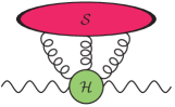
Figure 23: Pinch surfaces for the two-point function of an off-shell photon.

Extending soft and collinear power counting beyond one loop is not too cumbersome, and can be done by using a suitable generalisation of the techniques familiar from the analysis of UV divergences. Graphically, it is useful to introduce a diagrammatic notation for subgraphs, which we employ in Fig. 23 and in Fig. 24, and illustrate in what follows. In general, a coloured ‘blob’ denotes an arbitrary subgraph, where all lines are supposed to share a common kinematic constraint: for example, all lines in the jet subgraphs labelled $\mathcal{J}$ in Fig. 24 are collinear to the initial-state line entering the subgraph; similarly, all lines in the soft subgraphs labelled $\mathcal{S}$ in Figs. 23 and 24 have vanishing four-momenta, and all lines in the hard subgraphs labelled $\mathcal{H}$ are off the mass shell, and thus are contracted to a point in the reduced graph. When two subgraphs are connected by more than one line, it is understood (unless otherwise stated) that the number of such lines is arbitrary, with only a few being drawn for illustrative purposes.

To illustrate the rather formidable power of the apparently simple tools that we have just assembled, consider first the case of the two-point function for a massive particle, or for an off-shell massless particle such as the photon in Fig. 23, allowing for couplings to other massless particles such as gluons [61]. In this case, the CN analysis allows for no collinear pinch surfaces, since there are no massless external particles, and, if all couplings are to massless particles, there are no normal thresholds. One is left with only potential soft singularities, whose pinch surfaces are portrayed in Fig. 23. The next crucial step consists in identifying which of the pinch surfaces described by Fig. 23 give an actual infrared divergence. Thus, we need to find the superficial degree of infrared divergence $\omega_{s}$ for a generic soft pinch surface, adapting the power counting technique to the subgraph decomposition we have just discussed. In the case at hand, each soft-gluon loop in $d$ dimensions will provide $d$ powers of the soft momentum in the numerator, from the loop integration measure. Adding a gluon to the soft subgraph, however, is tantamount to adding a loop, and each gluon propagator will provide two powers of soft momentum in the denominator. Possible three-gluon couplings can only provide further powers of soft momentum in the numerator. For $N_{s}$ soft gluons we find then

$$\omega_{s}\,\geq\,(d-2)N_{s}\,.$$ (3.42)

In the case of infrared power counting, a divergence will arise only if $\omega_{s}\leq 0$: thus we have just proved that the two-point function is infrared finite for any $d>2$. Since the total cross section for electron-positron annihilation is given by the imaginary part of just this two-point function, thanks to unitarity, we have also proved that the cancellation of infrared divergences in the total cross section, demonstrated at one loop in Section 2, is actually verified to all perturbative orders. It is not difficult to extend this simple analysis to general massless correlators with euclidean momenta [2], which results in the Poggio-Quinn finiteness theorem [31, 32].

In the same spirit, the CN analysis for the form factor brings us to Fig. 24(a), which represents the generic diagram responsible for one of the pinch surfaces described in Section 3.1.4. Let us note at this point that the key aspects of the form factor analysis leading to Fig. 24(a) are in fact considerably more general, and remain valid beyond our specific example. In particular, for massless fixed-angle multi-particle amplitudes,

• the number of jet subgraphs must be at most equal to the number of hard particles involved, since jets must connect to external on-shell legs, and both incoming and outgoing particles may be affected by collinear emissions;
  

• with at most two incoming coloured particles, only one hard subgraph appears in the reduced diagram, and gives the meeting point of incoming and outgoing jets;
  

• particles belonging to different jets may interact only through soft mediators, which can be merged in a single soft subgraph.

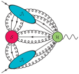
(a)

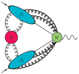
(b)

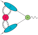
(c)

Figure 24: CN and power-counting analysis for the quark form factor. Panel $(a)$ displays soft, jet and hard subgraphs, connected by an arbitrary number of lines. Panel $(b)$ shows the subset of pinch surfaces contributing to IR divergences in Feynman gauge: double curly lines linking $\mathcal{J}_{i}$ and $\mathcal{H}$ denote scalar-polarised gluons. Panel $(c)$ displays singular surfaces in a physical gauge: in contrast with panel $(b)$, only a single line can connect $\mathcal{J}_{i}$ and $\mathcal{H}$.

In order to proceed to the power counting, it is important to devise a consistent treatment of the lines connecting the various subgraphs, in order to avoid double counting. One possibility [165] is to assign to the soft subgraph all loops containing at least one zero-momentum line, and to assign to jet subgraphs all loops containing only collinear lines with non-vanishing momentum. According to this criterion, for example, the loop in the reduced graph in Fig. 22(a) belongs entirely to the soft subgraph, and there are no collinear subgraphs, while the reduced diagram in the second panel of Fig 22(b) has only a jet subgraph and no soft subgraph. With these assignments, one can proceed to define soft and collinear superficial degrees of divergence, in terms of the numbers of loops and legs of each subgraph in Fig. 24(a). Let $L_{s}$ be the number of soft loops, and $L_{c,\,i}$ with $i=1,2$ the number of collinear loops in the $i$-th jet; similarly, let $N_{r}^{b}$ and $N_{r}^{f}$ be the numbers of bosonic and fermionic lines, respectively, in subgraph $r$, with $r=\{s,j_{1},j_{2}\}$. According to the scaling rules introduced in Section 3.2.2, in the soft limit bosonic propagators scale as $1/\lambda^{2}$, while fermion propagators scale as $1/\lambda$. In the collinear limit, both boson and fermions provide a factor of $1/\lambda$ (which may be corrected by numerator factors, as we will see below). Considering also the integration volume, that involves two normal coordinates for each collinear loop and four normal coordinates for each soft loop, we can define

$$\omega_{s} = 4L_{s}-2N_{s}^{b}-N_{s}^{f}+n_{s}\,,$$

$$\omega_{c,\,i} = 2L_{c,\,i}-N_{c,\,i}^{b}-N_{c,\,i}^{f}+n_{c,\,i}\,,$$ (3.43)

where $n_{s}$ and $n_{c,\,i}$ count positive powers of $\lambda$ arising from numerator factors. With our assignments, one readily verifies that $\omega_{s}=0$ for the reduced graph in Fig. 22(a), and $\omega_{c}=0$ for the reduced graph in the second panel of Fig. 22(b). In general, provided the lines connecting subgraphs have been consistently assigned, superficial degrees of divergence for subgraphs are additive. For a generic pinch surface $\Sigma$ for form factor graphs one can then define

$$\omega_{\Sigma}\,=\,\sum_{i=1}^{2}\omega_{c,\,i}+\omega_{s}\,.$$ (3.44)

The next step in the procedure is to rewrite Eq. (3.43) and Eq. (3.44) in terms of the numbers of vertices and external lines of the various subgraphs, using elementary graphical relations, such as the Euler identity connecting the numbers of loops, lines and vertices. There are a number of subtleties in the analysis: for example it is necessary to pay attention to the possible existence of lower-dimensional pinch surfaces in a given homogeneous integral, and to the fact that suppression factors for collinear numerators are polarisation-dependent, and thus gauge-dependent. The details of the procedure were worked out in Refs. [278, 279, 280], and are reviewed, for example, in Refs. [2, 61, 67, 281, 282]. In what follows, we will just provide a set of simple and, hopefully, intuitive arguments for the structure of the constraints emerging from power counting, and we will summarise the final results.

Consider for example the lines directly connecting the soft and hard subgraphs in Fig. 24(a): each such line would provide a power suppression, and they ultimately cannot contribute to divergent momentum configurations. To see that, let a soft gluon with momentum $k$ attach directly to a hard line carrying momentum $q\sim Q$, and assume that the graph contributes at leading power before the soft gluon is inserted. In case the hard line is a gluon, the corresponding off-shell propagator contributes a factor of $1/Q^{2}$ before the soft gluon insertion. After the insertion, the hard propagator is doubled, contributing a factor of $1/Q^{4}$, while the new three-gluon vertex can contribute at most a factor of $Q$: one has effectively gained a power suppression, which is sufficient to make the new graph finite if the graph was logarithmically divergent before the insertion. One can similarly argue that a graph with a soft fermion line connecting soft and jet subgraphs is suppressed by one power of the hard scale with respect to the same graph with a soft gluon, since soft fermion denominators are linear in the soft scaling parameter.

Turning now to numerator suppressions, we first note that in the soft limit the only source of suppression is the presence of three-gluon vertices, which are linear in momenta and thus provide a single power of $\lambda$ in the numerator: the suppression factor $n_{s}$ thus simply equals the number of soft three-gluon vertices. The situation concerning numerator suppressions in the collinear limit is much more subtle and interesting, since suppression factors are spin-dependent. In order to understand this, consider a fermion line carrying momentum $p$ and emitting a collinear gluon with momentum $k$. Both $p$ and $k$ can depend on collinear loop momenta, and thus they can have transverse components, which will however vanish in the collinear limit, where both particles reach the mass shell. The numerator factor associated with the emission vertex and the neighboring propagator reads

$$\left(\not{p}+\not{k}\right)\gamma_{\alpha}\,\not{p}\,=\,-\gamma_{\alpha}\left(\not{p}+\not{k}\right)\,\not{p}\,+\,2\left(p+k\right)_{\alpha}\,\not{p}\,.$$ (3.45)

In the collinear limit, $p$ and $k$ become light-like and the first term vanishes; as a consequence, away from the strict limit it will provide a power suppression proportional to $k_{\perp}$, i.e. a factor of $\sqrt{\lambda}$ for every collinear vertex. The second term in Eq. (3.45) does not provide any suppression, but one should keep in mind that the index $\alpha$ will be contracted with the neighbouring gluon propagator, whose numerator represents a sum over gluon polarisations; in the collinear limit, assuming the jet to be in the $+$ direction, the only surviving polarisation coupling to the vertex will be a $-$ component, which corresponds to an unphysical gluon. Such gluons would be absent in a physical gauge, and must decouple, after summing over diagrams, in a covariant gauge [61, 281]. To illustrate what happens in a physical gauge, note that a gluon connecting the jet subgraph to the hard (or soft) subgraph will carry a factor of the axial-gauge gluon propagator

$$G^{\mu\nu}(k)\,=\,\frac{1}{k^{2}+{\rm i}\eta}\left(-g^{\mu\nu}+\frac{n^{\mu}k^{\nu}+n^{\nu}k^{\mu}}{n\cdot k}-n^{2}\,\frac{k^{\mu}k^{\nu}}{(n\cdot k)^{2}}\right)\,,$$ (3.46)

where $n^{\mu}$ is the gauge vector, and the gauge condition imposes $n\cdot A=0$. As illustrated by Eq. (3.45), if the gluon connects the jet to the hard subgraph, at the vertex where $G^{\mu\nu}(k)$ attaches to the jet, it will be contracted with a collinear momentum, proportional to the gluon momentum $k$. This will yield a factor[61]

$$k_{\mu}G^{\mu\nu}(k)\,=\,\frac{1}{n\cdot k}\left(n^{\nu}-\frac{n^{2}k^{\nu}}{n\cdot k}\right)\,.$$ (3.47)

This factor has no pole at $k^{2}=0$ (except in the soft limit $k\sim 0$), so that such a graph is power-suppressed. In covariant gauges, the argument breaks down, since the contraction $k_{\mu}G^{\mu\nu}(k)$ does not feature the same suppression. For instance, in Feynman gauge, we have

$$k_{\mu}G^{\mu\nu}(k)\,=\,-\frac{k^{\nu}}{k^{2}}\,.$$ (3.48)

We see that in Feynman gauge multiple gluons may connect the jets subgraphs to hard subgraph $\mathcal{H}$, but Eq. (3.48) suggests that such gluons must carry unphysical polarisations. This, in turn, means that, when computing a gauge-invariant quantity, these configurations will be suppressed by means of the Ward Identity, when all the relevant diagrams have been summed. On a diagram-by-diagram basis, this is not guaranteed, and one needs to further manipulate the longitudinally polarised gluons to factor $\mathcal{J}_{i}$ from $\mathcal{H}$.

It is hopefully clear from these arguments that only a small subset of the pinch surfaces depicted in Fig. 24(a) will actually yield divergent contributions. A detailed analysis [2, 61, 67, 281] yields the following results.

1. The superficial degree of divergence $\omega_{\Sigma}$ is bounded by $\omega_{\Sigma}\geq 0$, implying that all infrared divergences are logarithmic. This has important consequences in what follows, since it means that even a single extra power suppression, such as those discussed above, makes the diagram superficially finite.

2. As a first consequence, pinch surfaces with lines directly connecting the soft subgraph $\mathcal{S}$ and the hard subgraph $\mathcal{H}$ are finite.

3. A second consequence is that only gluons can directly connect the soft subgraph $\mathcal{S}$ with the jet subgraphs $\mathcal{J}_{i}$.

4. Finally, in a physical gauge, in order to generate a divergence, every jet subgraph $\mathcal{J}_{i}$ must be connected to the hard subgraph $\mathcal{H}$ only by a single line (which must therefore carry the same quantum numbers as the external line entering or exiting the graph). In Feynman gauge, further additional lines linking $\mathcal{J}_{i}$ and $\mathcal{H}$ are allowed, but they must be scalar-polarised gluons. Furthermore one finds that, for each jet $\mathcal{J}_{i}$, the number of external soft gluons plus the number of jet gluons attached to the hard part cannot be greater than the total number of three-point vertices in that jet.

Graphically, these rules mean that pinch surfaces giving rise to divergences are considerably simpler than the general configuration depicted in Fig. 24(a), and they can be described by Fig. 24(b) in a covariant gauge (with double curly lines denoting scalar-polarised gluons), and by Fig. 24(c) in a physical gauge.

To summarise, we have learnt from power counting that sufficient conditions for the presence of infrared divergences are considerably more restrictive that the corresponding necessary conditions arising from the Landau equations and the CN physical picture. In axial gauges, Fig. 24(c) is already, effectively, a partially factorised expression for the form factor, separating the divergent subgraphs $\mathcal{S}$ and $\mathcal{J}_{i}$ from the finite subgraph $\mathcal{H}$. In Feynman gauge, we intuitively expect that Ward identities will drive a cancellation among diagrams that will ultimately lead to to a similar result. We can also hope to apply similar arguments to tame soft gluons attaching the soft subgraph to jet subgraphs. The third part of the analysis consists in examining in detail the actual Feynman rules in the relevant soft and collinear limits: this will enable us to leverage the universality of long-distance contributions, identifying operator matrix element that generate soft and collinear divergences for all fixed-angle scattering amplitudes, regardless of the particular hard process under consideration.

3.3 Diagrammatic construction of soft and collinear functions

Our next task is to turn the “quasi-factorisation” depicted in Fig. 24 (b) or (c) into an exact statement, writing the form factor (and later more general scattering amplitudes) as a product of functions, each responsible for the enhancements associated with specific kinematic configurations. This is still far from trivial, since what we have achieved so far is true for individual pinch surfaces, and the task ahead is to organise the contributions of all these pinch surfaces into universal operator matrix elements, that can be computed independently of the specific hard process under consideration. In other words, we want to identify matrix elements which share with the scattering amplitude specific sets of singularities, soft and/or collinear, so that the product of these matrix elements will contain all the infrared poles of the amplitude, leaving behind only a finite ‘matching coefficient’. If we succeed in identifying such matrix elements, we can then study infrared singularities to all orders, in a process-independent way, by means of evolution equations, as we will discuss in Section 4.

One way to identify the matrix elements we need is to consider soft and collinear approximations at the diagrammatic level, observe the systematic simplifications that arise in the relevant limits, and build the appropriate operators accordingly. A prominent role in this game will be played by Wilson-line operators, as we will see in some detail in Section 3.3.2.

3.3.1 Soft and collinear approximations at one loop

We begin by revisiting our one-loop results in Section 3.2.2, in particular the approximations leading to the soft and collinear homogeneous integrals in Eq. (3.32) and Eq. (3.2.2). At this level, we can easily generalise the results to the non-abelian theory, and, this time, we will pay closer attention to the numerator structures, which carry information about gluon polarisations, providing a more precise chracterisation of the result in Eq. (3.45). For this purpose, consider the annihilation process $q(p_{1})\,\bar{q}(p_{2})\rightarrow\gamma^{*}$. The un-approximated integral corresponding to the one-loop QCD correction to the QED vertex reads

$$\Gamma_{\mu}^{(1)}(p_{1},p_{2})\,=\,-eQ_{q}\int\frac{d^{d}k}{(2\pi)^{d}}\;\frac{\bar{v}(p_{2})\,\big{(}g\,T_{ij}^{a}\,\gamma^{\alpha}\big{)}\,\big{(}-p\hskip-4.49997pt/_{2}-k\hskip-4.49997pt/\big{)}\,\gamma_{\mu}\,\big{(}p\hskip-4.49997pt/_{1}-k\hskip-4.49997pt/\big{)}\,\big{(}g\,T_{jk}^{a}\,\gamma_{\alpha}\big{)}\,u(p_{1})}{\big{(}k^{2}+{\rm i}\eta\big{)}\,\big{[}(p_{2}+k)^{2}+{\rm i}\eta\big{]}\,\big{[}(p_{1}-k)^{2}+{\rm i}\eta\big{]}}\,.$$ (3.49)

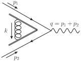
(a)

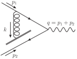
(b)

Figure 25: IR interactions modelled by eikonal Feynman rules. (a) Soft gluon exchange: both interaction vertices become eikonal. (b) Collinear exchange, with $k\parallel p_{1}$: only the vertex involving the antiquark line becomes eikonal.

In the soft limit, as was discussed already in Section 1.1, the homogeneous integral arises upon taking the eikonal approximation, amounting to

$$\frac{\big{(}\not{p}_{1}-\not{k}\big{)}\big{(}g\,T^{a}\,\gamma_{\alpha}\big{)}u(p_{1})}{(p_{1}-k)^{2}+{\rm i}\eta} \overset{k^{\mu}\to\,0}{\longrightarrow} \frac{g\,T^{a}\beta_{1,\alpha}}{-\beta_{1}\cdot k+{\rm i}\eta}\,u(p_{1})\,,$$

$$\frac{\bar{v}(p_{2})\big{(}g\,T_{a}\,\gamma^{\alpha}\big{)}\big{(}-\not{p}_{2}-\not{k}\big{)}}{(p_{2}+k)^{2}+{\rm i}\eta} \overset{k^{\mu}\to\,0}{\longrightarrow} \bar{v}(p_{2})\,\frac{-g\,T_{a}\,\beta_{2}^{\alpha}}{\beta_{2}\cdot k+{\rm i}\eta}\;,$$ (3.50)

where the Dirac equation has been used, and we took advantage of the scaling invariance of the approximation to replace the momenta $p_{1}$ and $p_{2}$ with the corresponding four-velocities using $p_{1}=\mu\beta_{1}$ and $p_{2}=\mu\beta_{2}$. Analogous replacements can be made for final-state fermions and anti-fermions, with due attention to overall signs and to the relative sign of the ${\rm i}\eta$ prescription: the results can be simply summarised in the eikonal Feynman rules

$${\rm propagator:}\quad\frac{\rm i}{\beta\cdot k+{\rm i}\eta}\,,\qquad\qquad{\rm vertex:}\quad{\rm i}g\,T_{a}\beta^{\alpha}\,,$$ (3.51)

with the convention that $\beta$ is the velocity flowing along the arrow of the fermion line, and $k$ is the soft momentum flowing in the same direction. Applying these Feynman rules one gets directly the expression for the soft homogeneous integral, Eq. (3.32), with the appropriate non-abelian prefactor.

As already noted in Section 1.1, these Feynman rules are independent of the spin and energy of the hard emitter, and only sensitive to its direction and colour charge. They apply at leading power in all soft momenta, which, by the power-counting arguments of Section 3.2, is all that is needed to capture soft divergences. We note now two further important properties of the eikonal approximation. First, the coupling to the colour charge is universal, in the sense that it is sufficient to replace the generator $T_{a}$ in the fundamental representation in Eq. (3.51) with the corresponding matrix $T^{r}_{a}$ in the representation $r$ of the gauge group, in order to reproduce the leading-power result if the emitter belongs to $r$ (for example, $(T_{a})_{bc}\to-{\rm i}f_{abc}$ in the adjoint representation): we will take advantage of this universality property in Section 5. Second, we note that, taking the hard momentum in a fixed direction, say $\beta=\{\beta^{+},0^{-},{\bf 0}_{\perp}\}$ in light-cone coordinates, the eikonal coupling of the soft gluon to the hard line involves only the $-$ component of its polarisation at leading power. Furthermore, if all components of the soft gluon momentum scale equally in the soft limit, according to Eq. (3.33), the only component of the gluon momentum which is relevant at leading power is $k^{-}$. Soft gluons thus couple longitudinally to hard lines, a fact which will be instrumental in what follows. The simplified coupling of soft lines to hard lines is shown pictorially in Fig 25 (a), where eikonal vertices are represented as the merging of gluon propagator with a double line.

In the same spirit, let’s revisit the collinear approximation, leading to the collinear homogeneous integral in Eq. (3.2.2), focusing on the numerator structure. In the frame in which $p_{1}^{\mu}$ in in the $+$ direction, while $p_{2}^{\mu}$ is in the $-$ direction, the integrand reads

$$T^{a}\,T_{a}\,\frac{\bar{v}(p_{2})\gamma^{-}\big{(}p\hskip-4.49997pt/_{2}+\not{k}\big{)}\,\gamma^{\mu}\big{(}p\hskip-4.49997pt/_{1}-k\hskip-4.49997pt/\big{)}\,\gamma^{+}u(p_{1})}{\big{[}k^{2}+{\rm i}\eta\big{]}\;\big{[}(p_{1}-k)^{2}+{\rm i}\eta\big{]}\;\big{[}(p_{2}+k)^{2}+{\rm i}\eta\big{]}}\,,$$ (3.52)

where we used the massless Dirac equations in this frame, which read $\bar{v}(p_{2})\gamma^{+}=\gamma^{-}u(p_{1})=0$. By the same token, and using the fact that, in the region collinear to $p_{1}$, the $k^{-}$ component of the loop momentum is power-suppressed, we can approximate the numerator of Eq. (3.52) using

$$\bar{v}(p_{2})\gamma^{-}\big{(}p\hskip-4.49997pt/_{2}+\not{k}\big{)}\,\simeq\,(p_{2}+k)^{-}\;\bar{v}(p_{2})\gamma^{-}\gamma^{+}\,=\,2(p_{2}+k)^{-}\,\bar{v}(p_{2})\,\simeq\,2\,p_{2}^{-}\,\bar{v}(p_{2})\,.$$ (3.53)

In the collinear approximation, Eq. (3.52) can then be rewritten as

$$T^{a}\,T_{a}\,\frac{\bar{v}(p_{2})\,\gamma^{\mu}\big{(}\not{p}_{1}-\not{k})\gamma_{\alpha}\,u(p_{1})}{k^{2}(p_{1}-k)^{2}}\;\frac{\beta_{2}^{\alpha}}{\beta_{2}\cdot k}\;.$$ (3.54)

Remarkably, the vertex attaching the collinear gluon to the anti-quark has become eikonal, and can be expressed in terms of the effective Feynman rules of Eq. (3.51), as represented pictorially in Fig. 25 (b). As before, the gluon coupling to the anti-quark has become independent of the anti-quark energy; furthermore, the gluon couples to the antiquark with a polarisation parallel to its momentum: it is longitudinal, and thus unphysical. On the other hand, the coupling of the collinear gluon to the quark has not simplified, and retains its spin and energy dependence.

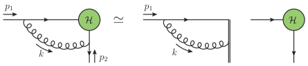
Figure 26: Factorisation of the hard subgraph after a collinear emission. Notice that the collinear prefactor is a spin matrix, as discussed in the text.

In view of generalising this result to higher perturbative orders, it is useful to note that the sequence of approximations leading to Eq. (3.54) can be reformulated as the application of a tree-level Ward identity. Let us assume to have a longitudinally polarised gluon moving in the $+$ direction, and attaching to a generic hard interaction subgraph $H$. Writing the (Feynman-gauge) numerator of the gluon propagator as a sum over polarisations, including unphysical ones, the amplitude for this process is of the form

$$\sum_{\lambda}\,\bar{v}(p_{2})\gamma_{\alpha}\frac{\not{p}_{2}+\not{k}}{(p_{2}+k)^{2}+{\rm i}\eta}\,\varepsilon^{\alpha}_{(\lambda)}(k)\,H\,\varepsilon^{*\beta}_{(\lambda)}(k)\frac{\not{p}_{1}-\not{k}}{(p_{1}-k)^{2}+{\rm i}\eta}\,\gamma_{\beta}\,u(p_{1})\,,$$ (3.55)

where the hard subgraph $H$ is defined here to include the denominator of the gluon propagator and we can focus on the case of longitudinal polarisation. We can then substitute $\not{\varepsilon}_{(\lambda)}(k)=\gamma^{-}\varepsilon^{+}(k)$, and insert a factor of $1=k^{+}\beta_{2}^{-}/k^{+}\beta_{2}^{-}$, so that Eq. (3.55) becomes [283]

$$\frac{k^{+}\beta_{2}^{-}}{k^{+}\beta_{2}^{-}}\,\bar{v}(p_{2})\,\gamma^{-}\frac{\not{p}_{2}+\not{k}}{(p_{2}+k)^{2}+{\rm i}\eta}\,\varepsilon^{+}(k)\,H\,\frac{\not{p}_{1}-\not{k}}{(p_{1}-k)^{2}+{\rm i}\eta}\,\not{\varepsilon}(k)\,u(p_{1})$$ (3.56)

$$= \frac{\varepsilon(k)\cdot\beta_{2}}{k\cdot\beta_{2}}\;\bar{v}(p_{2})\,\not{k}\,\frac{\not{p}_{2}+\not{k}}{(p_{2}+k)^{2}+{\rm i}\eta}\,H\,\frac{\not{p}_{1}-\not{k}}{(p_{1}-k)^{2}+{\rm i}\eta}\,\not{\varepsilon}(k)\,u(p_{1})$$

$$= \bar{v}(p_{2})\,H\,\frac{\varepsilon(k)\cdot\beta_{2}}{k\cdot\beta_{2}}\frac{\not{p}_{1}-\not{k}}{(p_{1}-k)^{2}+{\rm i}\eta}\,\not{\varepsilon}(k)\,u(p_{1})\,,$$

where in the last step we have used $\not{k}=-\not{p}_{2}+(\not{p}_{2}+\not{k})$: the first term then vanishes by the Dirac equation, and the second term cancels the denominator of the antiquark propagator, effectively replacing it with the eikonal denominator. One then readily recognises Eq. (3.54). Thanks to this ‘Ward identity’, we can effectively write the amplitude as the product of a spin factor with an eikonal coupling to the antiquark, multiplying the hard subgraph, as depicted in Fig. 26.

To summarise the results of this one-loop analysis, we have seen that a soft gluon couples eikonally to all hard lines, while a collinear gluon couples eikonally to anti-collinear hard lines. Eikonal couplings are energy- and spin-independent, and, more interestingly, involve unphysical polarisations at leading power. This observation is the key to the generalisation of this result to higher orders in perturbation theory: the only effect of unphysical gluons is to dress the hard particles with a gauge rotation. The framing of the one-loop collinear limit in the language of diagrammatic Ward identities suggests how to proceed at higher orders: in case of multiple radiations, the number of possible collinear connections to the hard subgraph increases, however the Ward identity will guarantee that the eikonal approximation on the anticollinear line still holds, and all emissions can be expressed in terms of effective Feynman rules. This was already established for abelian soft radiation in Section 1.1. In the non-abelian theory, further care must be taken in order to insure that the colour ordering of the attachments is consistently reproduced: as we will see in the next section, there is a natural solution to this problem. We must however note an important caveat in the non-abelian case: at higher orders, soft gluons will couple to a set of collinear lines (rather than a single line), which in general will have momenta with small transverse components. Couplings of soft gluons to these components will be negligible only if the soft limit is taken at the same rate for all components of the soft momentum $k$, as in Eq. (3.33). In a momentum region where $k^{-}$ is much smaller that $k_{\perp}$, the approximation that we have made in order to effectively factorise soft lines from ‘jet’ lines may fail. We will briefly return to this issue in Section 5. A more detailed description of the all-order proof of the factorisation of soft lines from hard collinear ones is given in Ref. [61], while a full analysis can be found in Ref. [67].

3.3.2 Wilson lines and the eikonal approximation

Power counting and diagrammatic analyses have given us a much-simplified picture of soft and collinear radiation. Specifically, we have seen that only limited physical information links soft, hard and collinear subgraphs. Our next step is to identify operator matrix elements that contain this same information, and therefore share the same singular regions in loop-momentum space. Before we proceed, however, it is important to pause and focus on the physical underpinnings of our conclusions so far. A crucial ingredient of the factorisation is the fact that soft radiation is insensitive to the nature of hard exchanges, as well as to the internal structure of collinear jets of fast particles: only the overall direction of the collinear beam and its overall colour charge can be detected by soft gluons. This is a consequence of the fact that soft radiation has long wavelength, which cannot discriminate the short-distance features of the scattering process, or the fine structure of collimated jets. This simple physical fact is not directly apparent from individual Feynman diagrams, and only emerges, at high orders, after intricate cancellations. It has however been well-understood for a long time, under the heading of colour transparency, first discussed in the non-abelian theory in Refs. [284, 285], and reviewed for example in Refs. [286, 287]. This in turns forms the basis for the colour coherence approach, one of the first powerful tools for all-order analyses in perturbative QCD (see, for example, [288, 289, 290, 291, 292]). For collinear radiation, we have observed a similar phenomenon: collinear gluons are sensitive to the spin and energy of the emitter, but cannot resolve the quantum numbers of anti-collinear particles. The axial-gauge result, showing that only a single particle can connect jets to the hard scattering, which in turn is reflected by the eikonal couplings of scalar-polarized collinear gluons in covariant gauges, also implies that hard collinear radiation depends on the colour charge of the collinear beam, but is not sensitive to colour exchanges with other hard particles: the only long-distance colour exchanges between different hard particles are effected by soft gluons.

We now turn to the construction of matrix elements reproducing these physical results, expressed by eikonal Feynman rules. In the soft case, a natural guess leads to the correct ansatz: at leading power in the soft radiation, hard particles do not recoil, and follow straight-line trajectories from the hard scattering point out to time-like infinity, in a specified direction. Along these trajectories, soft interactions can only dress the hard particle with a gauge phase. This phase in turn is naturally expressed by integrating the gauge connection along the trajectory. The required operator, for each hard particle, is therefore a straight Wilson line, defined in general by

$$\Phi_{n}(\lambda_{2},\lambda_{1})\,=\,\mathcal{P}\exp\bigg{[}{\rm i}g\int_{\lambda_{1}}^{\lambda_{2}}d\lambda\;n\cdot A^{a}(\lambda n)\,T_{a}\bigg{]}\;,$$ (3.57)

where $n^{\mu}$ is the direction of the line, and, in the non-abelian case, one needs to introduce the path ordering operator $\mathcal{P}$. Eq. (3.57) is a colour matrix in the representation of the selected hard particle. In the present context, we will only need semi-infinite lines, with $\lambda_{1}=0$ and $\lambda_{2}=\infty$. It is not difficult to convince oneself that Wilson lines reproduce eikonal Feynman rules, and the path-ordering provides the correct non-abelian generalisation of the eikonal approximation.

To this end, consider, for example, a graph $G$ featuring an outgoing on-shell hard quark line carrying momentum $p$, emitting an arbitrary number $n$ of low-energy gluons with colour indices $a_{i}$ and carrying momenta $k_{i}$. At leading power in all soft momenta, we can simply adapt Eq. (1.17) to include color operators, and we obtain the expression

$$G^{\,a_{1}\dots a_{n}}_{\mu_{1}\dots\mu_{n}}\big{(}\,p,\{k_{i}\}\big{)}\,\simeq\,\prod_{i=1}^{n}\;\left[\big{(}{\rm i}g\,T^{a_{i}}\big{)}\frac{i\,p^{\mu_{i}}}{p\cdot\left(\sum_{j=1}^{i}k_{j}\right)}\right]\bar{u}(p)\,{\cal M}\big{(}p\big{)}\;.$$ (3.58)

In the abelian case, it was possible to sum explicitly over the permutations of the outgoing gluons, so that Eq. (3.58) could be simplified by applying the eikonal identity, Eq. (1.18). The identity, however, expresses the fact that successive photon emissions are independent and uncorrelated in the abelian theory, and is no longer valid in the non-abelian case, since the colour matrices do not commute. This, in turn, requires the path-ordering prescription in Eq. (3.58).

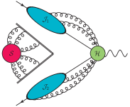
(a)

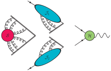
(b)

Figure 27: Different steps of the factorisation procedure. a) Factorisation of the soft subgraph: multiple soft gluon emissions are modelled via eikonal Feynman rules. b) Factorisation of the jet subgraph from the hard part: collinear gluons attach to eikonal vertices

To verify that the momentum-space eikonal Feynman rules are reproduced, it is sufficient to expand the definition in Eq. (3.57), and Fourier transform the gauge field, according to

$${A_{\mu}^{a}(\lambda n)\,=\,\int\frac{d^{d}k}{(2\pi)^{d}}\;e^{{\rm i}k\cdot\lambda n}\tilde{A}_{\mu}^{a}(k)}\,.$$ (3.59)

At leading order the expansion gives

$${\cal P}\exp\bigg{[}\,{\rm i}g\int_{0}^{\infty}d\lambda\,n\cdot A^{a}(\lambda n)\,T_{a}\bigg{]}\,=\,1-g\int\frac{d^{d}k}{(2\pi)^{d}}\,\frac{n\cdot\tilde{A}^{a}(k)}{n\cdot k+{\rm i}\eta}\,\,T_{a}+{\cal O}(g^{2})\,,$$ (3.60)

where we used Feynman’s prescription to define the parameter integral at large distances, resulting in

$$\int_{0}^{\infty}d\lambda\,{\rm e}^{{\rm i}(k\cdot n)\lambda}\,\to\,\int_{0}^{\infty}d\lambda\,{\rm e}^{{\rm i}(k\cdot n+{\rm i}\eta)\lambda}\,=\,\frac{{\rm i}}{k\cdot n+{\rm i}\eta}\,,$$ (3.61)

reflecting the Feynman rules in Eq. (3.51). At the next order in the expansion the path-ordering prescription becomes relevant, yielding the correct partial denominators of Eq. (3.58). Indeed one finds

$$\big{(}{\rm i}g\big{)}^{2}\int_{0}^{\infty}\!d\lambda_{1}\int_{0}^{\lambda_{1}}\!d\lambda_{2}\,n\cdot A^{a}(\lambda_{1}n)\,n\cdot A^{b}(\lambda_{2}n)\,T_{a}\,T_{b}$$

$$=\,\big{(}{\rm i}g\big{)}^{2}\,\int\frac{d^{d}k_{1}}{(2\pi)^{d}}\frac{d^{d}k_{2}}{(2\pi)^{d}}\int_{0}^{\infty}\!d\lambda_{1}\int_{0}^{\lambda_{1}}\!d\lambda_{2}\,{\rm e}^{{\rm i}(\lambda_{1}k_{1}+\lambda_{2}k_{2})\cdot n}\,n\cdot\tilde{A}^{a}(k_{1})\,n\cdot\tilde{A}^{b}(k_{2})\,T_{a}\,T_{b}$$

$$=\,g^{2}\!\int\frac{d^{d}k_{1}}{(2\pi)^{d}}\frac{d^{d}k_{2}}{(2\pi)^{d}}\,\frac{n\cdot\tilde{A}^{a}(k_{1})}{k_{1}\cdot n+{\rm i}\eta}\,\frac{n\cdot\tilde{A}^{b}(k_{2})}{(k_{1}+k_{2})\cdot n+{\rm i}\eta}\,T_{a}\,T_{b}\,,$$ (3.62)

which is fully consistent with the diagrammatic expression of a double emission. The pattern in Eq. (3.62) generalises to all orders, yielding

$$\mathcal{P}\exp\left[\,{\rm i}g\,T_{a}\int_{0}^{\infty}d\lambda\,n\cdot A^{a}(\lambda n)\right]\,=\,1+\sum_{n=1}^{\infty}\left[\,\prod_{i=1}^{n}\left(\int\frac{d^{d}k_{i}}{(2\pi)^{d}}\frac{g\,T_{a_{i}}\,n\cdot\tilde{A}^{a_{i}}(k_{i})}{\sum_{j=1}^{i}n\cdot k_{i}+{\rm i}\eta}\right)\,\right]\,,$$ (3.63)

which reproduces the leading-power result for soft gluon attachments to a hard line, exemplified in Eq. (3.58).

These results confirm our intuition, that the interactions of a hard particle as it propagates in a background of soft gluons without recoil are correctly reproduced by replacing the particle with an appropriate Wilson-line operator. Interactions between different hard particles propagating in different directions and exchanging soft gluons will similarly be reproduced by taking a vacuum expectation value of a set of Wilson lines, each in the appropriate representation of the gauge group, and defined along the classical straight-line trajectory of the hard emitter. The path-integral evaluation of the resulting correlator will automatically generate all the radiative corrections building up the generic soft subgraphs discussed in the previous sections. To illustrate these facts in the simplest case, we can easily reproduce the expression of the one-loop eikonal integral in Eq. (2.39) by considering the correlator of two Wilson lines. Writing explicitly the open colour indices, we find

$$\left\langle\smash{0}{\vphantom{1}}\right|{\rm T}\,\Big{[}\Phi^{f_{1}g_{1}}_{\beta_{1}}(\infty,0)\,\Phi^{f_{2}g_{2}}_{\beta_{2}}(\infty,0)\Big{]}\left|\smash{0}{\vphantom{1}}\right\rangle$$

$$=\,1\,-\,g^{2}\,\big{(}T_{1}^{a}\big{)}^{f_{1}g_{1}}\,\big{(}T_{2}^{b}\big{)}^{f_{2}g_{2}}\,\beta_{1}^{\mu}\beta_{2}^{\nu}\int_{0}^{\infty}d\lambda_{1}\,d\lambda_{2}\,\left\langle\smash{0}{\vphantom{1}}\right|{\rm T}\,\Big{[}A_{\mu}^{a}(\lambda_{1}\beta_{1})\,A_{\nu}^{b}(\lambda_{2}\beta_{2})\Big{]}\left|\smash{0}{\vphantom{1}}\right\rangle\,+\,\ldots$$

$$=\,1\,-g^{2}\,\big{(}T_{1}^{a}\big{)}^{f_{1}g_{1}}\,\big{(}T_{2}^{b}\big{)}^{f_{2}g_{2}}\,\beta_{1}^{\mu}\beta_{2}^{\nu}\int_{0}^{\infty}d\lambda_{1}\,d\lambda_{2}\,\int\frac{d^{d}k}{(2\pi)^{d}}\,\bigg{(}\frac{-{\rm i}g_{\mu\nu}\,\delta^{ab}}{k^{2}+{\rm i}\eta}\bigg{)}\,{\rm e}^{{\rm i}k\cdot(\lambda_{1}\beta_{1}-\lambda_{2}\beta_{2})}\,+\,\ldots$$

$$=\,1\,+\,{\rm i}g^{2}\,T_{1}\cdot T_{2}\,\beta_{1}\cdot\beta_{2}\int\frac{d^{d}k}{(2\pi)^{d}}\,\frac{1}{(k^{2}+{\rm i}\eta)(k\cdot\beta_{1}-{\rm i}\eta)(k\cdot\beta_{2}+{\rm i}\eta)}\,+\,\ldots\,.$$ (3.64)

We omitted self-energy corrections, which arise by expanding one of the two Wilson lines to ${\cal O}(g^{2})$, and vanish in a massless theory, where the Wilson lines lie on the light cone. In the second line of Eq. (3.3.2) we recognised the coordinate-space gluon propagator, and in the last line we performed the parameter integrals, and we defined the scalar product $T_{1}\cdot T_{2}\equiv T_{1}^{a}T_{2,\,a}$. We note that one could also perform the calculation by using the explicit expression of the coordinate-space gluon propagator: this possibility is exploited and discussed in detail in Section 5. We recognise the result of Eq. (2.39), but this time with open colour indices, which can later be contracted with open colour indices of the hard matching function.

The arguments above represent an important step forward on the way to a complete infrared factorisation for form factors, and later for fixed-angle scattering amplitudes: having identified a set of operator matrix elements (such as Eq. (3.3.2)) that reproduce all the leading-power soft singularities of the form factor, we can promote the diagrammatic factorisation represented in Fig. 24, where subgraphs are still linked by colour and spin indices, to the complete factorisation depicted in Fig. 27(a), where we can now interpret the double lines as Wilson lines, and the soft subgraph is promoted to a soft function,

$$\langle 0|T\Big{[}\Phi_{\beta_{1}}(\infty,0)\,\Phi_{\beta_{2}}(\infty,0)\Big{]}|0\rangle\,,$$ (3.65)

responsible for all divergent configuration originating from soft gluons. Hard and collinear integration regions will of course be misrepresented by the soft function, and will have to be included in other terms in the factorisation.

As far as collinear regions are concerned, the discussion leading to Eq. (3.54) provides a clear suggestion for how to proceed: collinear gluons couple eikonally to anti-collinear lines, so we can build a jet function by replacing anti-collinear lines by a Wilson line, while retaining spin and colour information for the emitting collinear line. This results in the further factorisation depicted in Fig. 27 (b). Tentatively, one could introduce an object of the form

$$\langle 0\,|\,\Phi_{\beta_{2}}(0,\infty)\,\psi(0)\,|p_{1},s_{1}\rangle\,,$$ (3.66)

where a quark of momentum $p_{1}$ and spin polarisation $s_{1}$ in the initial state is annihilated by the quark field at the origin, and a Wilson line replaces the incoming antiquark. This function, however, has the drawback that it still contains collinear divergences associated with the antiquark, since the Wilson line is light-like in the massless case, and gluons attaching to it will have anti-collinear enhancements, not fully matching those of the original amplitude. The solution in this case is very simple: we can just replace the light-like Wilson line along the $\beta_{2}$ direction with a ‘massive’ Wilson line with a direction $n^{\mu}$, with $n^{2}\neq 0$. The resulting function will have the correct collinear singularities associated with the quark direction, but only finite contributions from the anti-collinear momentum region. As before, the resulting function will again misrepresent the soft and hard momentum integration regions, which are correctly approximated by other terms in the factorisation. In particular, we note that gluons that are both soft and either collinear or anti-collinear are correctly approximated both in the soft and in the collinear factors. Including both factors will result in double-counting, and will require a subtraction. In the next section, we will tackle these issues, and we will provide a complete picture of infrared factorisation for form factors.

4 Factorisation, evolution and resummation: form factors

The tools developed in Section 3 have motivated, if not proved in detail, a factorisation formula for form factors, where all soft and collinear divergences are accounted for in terms of universal function, which can be expressed as matrix elements of fields and Wilson lines. This factorisation formula will be discussed in greater detail in Section 4.1. For the moment, we wish to emphasise that, once the hard work of proving factorisation has been completed, there are low-hanging fruits to be reaped: every factorisation theorem, in fact, implies a set of evolution equations, and the solution of these equation leads to a partial summation of perturbation theory. Before we apply this to soft-collinear factorisation of scattering amplitudes, we wish to recall briefly how this happens in standard applications, following [293].

The simplest and best known example of this process is of course the renormalisation of UV divergences, which amounts to the factorisation of singular cutoff dependence into a finite set of universal renormalisation constants. Assuming that perturbative renormalisability has been proven for the theory at hand, consider the relation between bare and renormalised Green functions,

$$G_{0}^{(n)}\big{(}p_{i},\Lambda,g_{0}\big{)}\,=\,\prod_{i=1}^{n}\,Z_{i}^{1/2}\bigg{(}\frac{\Lambda}{\mu},g(\mu)\bigg{)}\,G_{R}^{(n)}\big{(}p_{i},\mu,g(\mu)\big{)}\,,$$ (4.1)

where $Z_{i}$ are renormalisation constants for the fields appearing in the correlator, $g_{0}$ is a bare coupling, $\Lambda$ is an ultraviolet cutoff (for example the inverse of a lattice spacing), and $\mu$ is the renormalisation scale. Proving that Eq. (4.1) holds, possibly with the added burden of showing that other useful properties of the theory, such as unitarity, or gauge symmetry, are preserved, is in general difficult. When this has been achieved, however, one can mine Eq. (4.1) for further information. In order to achieve the factorisation, it is strictly necessary to introduce a additional energy scale, $\mu$, which, intuitively, we place somewhere between the laboratory energy scales, given by the Mandelstam invariants $p_{i}\cdot p_{j}$, and the cutoff scale. Renormalisability means that all singular cutoff dependence is confined to the field renormalisation constants $Z_{i}$. Once that is established, a (Callan-Symanzik) evolution equation immediately follows, by simply noting that the l.h.s of Eq. (4.1) does not depend on the renormalisation scale $\mu$, which has been introduced as a necessary artefact of renormalisation. Scale dependence must therefore cancel between the factors on the r.h.s., so that

$$\frac{dG_{0}^{(n)}}{d\mu}\,=\,0\,\qquad\longrightarrow\qquad\frac{d\log G_{R}^{(n)}}{d\log\mu}\,=\,-\sum_{i=1}^{n}\gamma_{i}\big{(}g(\mu)\big{)}\,,$$ (4.2)

where the anomalous dimensions $\gamma_{i}$ are defined by

$$\gamma_{i}\big{(}g(\mu)\big{)}\,\equiv\,\frac{1}{2}\,\frac{d\log Z_{i}}{d\log\mu}\,.$$ (4.3)

The simple functional dependence of the anomalous dimensions is dictated by separation of variables in Eq. (4.2): $\gamma_{i}$ cannot depend on the cutoff $\Lambda$, because the renormalised Green function $G_{R}^{(n)}$ does not, and it cannot depend on the momenta $p_{i}$, because $Z_{i}$ does not. Anomalous dimensions can only depend on arguments that are in common between the l.h.s. and the r.h.s. of Eq. (4.2), in this case just on the renormalised coupling $g(\mu)$. Armed with an evolution equation, one can solve it, and, in this case, ‘resum’ logarithms of the renormalisation scale $\mu$. Since the renormalised Green function $G_{R}^{(n)}$ depends on $\mu$ through the coupling and through ratios of the form $p_{i}\cdot p_{j}/\mu^{2}$, solving the equation gives precious information on the dependence of the correlator on external energy scales.

A second standard example of the same phenomenon is collinear factorisation in high-energy scattering, which we briefly introduced in Section 2.8. Eq. (2.62) is an all-order factorisation theorem, which can be proved in perturbation theory either by hard diagrammatic work, or by using more sophisticated tools such as the light-cone expansion. It states that collinearly enhanced contributions can be factored from the cross section in the form of a convolution, and can be organised into a set of parton distribution functions $f_{j/i}$. If desired, the convolution can be diagonalised by a Mellin transform, using the definition

$$\widetilde{W}(N)\,\equiv\,\int_{0}^{1}z^{N-1}\,W(z)\,.$$ (4.4)

Applying this definition to Eq. (2.62), for a single particle flavour, results in the simple factorisation

$$\widetilde{W}\bigg{(}N,\frac{Q^{2}}{m^{2}},\alpha_{s}(Q^{2})\bigg{)}\,=\,\widetilde{H}\bigg{(}N,\frac{Q^{2}}{\mu_{f}^{2}},\alpha_{s}(Q^{2})\bigg{)}\,\widetilde{f}\bigg{(}N,\frac{\mu_{f}^{2}}{m^{2}},\alpha_{s}(Q^{2})\bigg{)}\,,$$ (4.5)

where $Q$ is the hard scale, we used a particle mass $m$ as a collinear regulator, replacing dimensional regularisation, and we noted that the factorisation procedure requires the introduction of a factorisation scale $\mu_{f}$. In Eq. (4.5), the singular dependence on the collinear cutoff $m$ is collected in the (Mellin-space) parton distribution $\widetilde{f}$, while the Wilson coefficient $\widetilde{H}$ is free of singularities as $m\to 0$. Also in this case, DGLAP evolution follows from the observation that the full partonic structure function does not depend on the factorisation scale. Then

$$\frac{d\widetilde{W}}{d\mu_{f}}\,=\,0\,\qquad\longrightarrow\qquad\frac{d\log\widetilde{f}}{d\log\mu_{f}}\,=\,-\,\gamma_{N}\big{(}\alpha_{s}(Q^{2})\big{)}\,,$$ (4.6)

where

$$\gamma_{N}\big{(}\alpha_{s}(Q^{2})\big{)}\,\equiv\,\frac{d}{d\log\mu_{f}}\,\widetilde{H}\bigg{(}N,\frac{Q^{2}}{\mu_{f}^{2}},\alpha_{s}(Q^{2})\bigg{)}\,.$$ (4.7)

Once again, the anomalous dimension $\gamma_{N}$ (the Mellin transform of the DGLAP splitting function) can depend only on variables that are common to the two factors on the r.h.s. of Eq. (4.5), in this case $N$ and $\alpha_{s}$. Solving the DGLAP equation leads to the resummation of collinear logarithms, which effectively disappear from the calculation of the DIS cross section, as they are absorbed into the parton distribution evaluated at the proper scale.

Soft-collinear factorisation of scattering amplitudes generalises these familiar examples. Considering the form factor as a first example, we note that a double factorisation has been performed, extracting a soft factor, and a collinear factor for each external leg. We expect therefore two evolution equations, matching the double-logarithmic nature of the amplitude we are considering. This is indeed what we will find, after examining the factorisation in more detail.

4.1 Soft-collinear factorisation of a form factor

Let us summarise the path that leads to the soft-collinear factorisation of the form factor, as outlined in Section 3. First, the Landau equations, as implemented in the Coleman-Norton physical picture, identify soft and collinear gluons as the only potential source of divergences in the (renormalised) massless form factor. Next, power counting reveals that the connections between hard, soft and collinear subdiagrams are strongly constrained: at leading power in the normal variables, no lines can directly connect soft and hard factors; in a physical gauge, only one line can connect collinear and hard factors (while in a covariant gauge this line can be supplemented by any number of scalar-polarised gluons, which however decouple from the hard subgraph after summing over diagrams, by means of the Ward identity); soft gluons at wide angles couple to collinear lines only with the anti-collinear components of their momenta, and they are longitudinally polarised along the anti-collinear direction, so that they effectively couple to a single Wilson line along the jet direction. The last step in Section 3 was the use of explicit diagrammatic arguments in order to identify operator matrix elements carrying the same singularities as the form factor in the soft and collinear sectors. This led to the identification of the soft function as a matrix element of light-like Wilson lines extending along the classical trajectories of the incoming particles. Taking as an example an incoming quark-antiquark pair, we define then

$${\cal S}\left(\beta_{1}\cdot\beta_{2},\alpha_{s}(\mu^{2}),\epsilon\right)\,\equiv\,\langle 0|T\Big{[}\Phi_{\beta_{1}}(\infty,0)\,\Phi_{\beta_{2}}(\infty,0)\Big{]}|0\rangle\,.$$ (4.8)

Similarly, for collinear singularities, after the decoupling from the anti-collinear line and from wide-angle soft gluons, it becomes clear that collinear divergences are uniquely associated with each incoming hard particle, and they can be simulated with a jet function of the form

$${\cal J}\bigg{(}\frac{(p\cdot n)^{2}}{n^{2}\mu^{2}},\alpha_{s}(\mu^{2}),\epsilon\bigg{)}u_{s}(p)\,\,\equiv\,\langle 0\,|\,T\Big{[}\Phi_{n}(\infty,0)\,\psi(0)\Big{]}\,|p,s\rangle\,,$$ (4.9)

and a similar one for the antiquark. Contrary to the soft function in Eq. (4.8), the jet function in Eq. (4.9) does not contain colour correlations between the quark and the antiquark, but it is spin-dependent. In general, one will also need a definition for a gluon jet function: in order to provide it, one cannot simply replace the quark field by a gluon field in Eq. (4.9), since the result would not be gauge invariant. A possible definition bypassing this problem was proposed in [294, 295], and is given by

$$g\,{\cal J}_{g}^{\mu\nu}\!\left(\frac{(k\cdot n)^{2}}{n^{2}\mu^{2}},\alpha_{s}(\mu^{2}),\epsilon\right)\,\varepsilon^{(\lambda)}_{\mu}(k)\,\equiv\,\left\langle\smash{0}{\vphantom{1}}\right|T\Big{[}\Phi_{n}(\infty,0)\,{\rm i}D^{\nu}\,\Phi_{n}(\infty,x)\Big{]}\left|\smash{k,\lambda}{\vphantom{1}}\right\rangle\Big{|}_{x=0}\,,$$ (4.10)

where the Wilson line in the $n$ direction acts directly as the gluon source.

Finally, we turn to the issue of subtracting the potential double counting of the momentum regions involving gluons that are both soft and collinear to the incoming partons. Such regions indeed appear both in the soft function in Eq. (4.8) and in the jets, Eqns. 4.9 and 4.10. It would appear to be non-trivial to subtract collinear configurations from the soft function, however the simple form of the jet functions leads to a straightforward proposal for subtracting their soft limits: one may simply divide each jet by its own soft approximation, which is naturally given by a very similar matrix element, with the field of the hard parton replaced by its own Wilson line. Thus we define the eikonal jet function

$${\cal J}_{\rm E}\bigg{(}\frac{(\beta\cdot n)^{2}}{n^{2}},\alpha_{s}(\mu^{2}),\epsilon\bigg{)} \equiv \langle 0|T\Big{[}\,\Phi_{\beta}(\infty,0)\,\Phi_{n}(\infty,0)\Big{]}\,|0\rangle\,.$$ (4.11)

As expected from the general properties of the soft approximation, eikonal jets are independent of spin, and they depend on colour only through the representation in which the Wilson lines are defined. The fact that the proper way to ‘subtract’ the soft-collinear region is to divide by the eikonal jets will be better justified in what follows, where we will see that jet and eikonal jet functions exponentiate, and they are normalised to unity at lowest order: by taking a ratio, we are effectively subtracting their perturbative exponents.

Not suprisingly, closely related definitions of soft and jet functions arise in the SCET approach to infrared factorisation (see, for example, Refs. [75, 92, 95, 96, 296]), and they have been extensively investigated both at amplitude and at cross-section level. In the context of SCET, soft and jet functions are defined in terms of soft and collinear fields, which directly enter the SCET lagrangian. Practical calculations at leading power in the two formalisms are closely related, but the double-counting problem for the soft-collinear region is dealt with in a different way, using the so-called zero-bin subtraction, discussed for example in Refs. [326, 327, 328, 329].

Before making several comments about the physical meaning and implications of our definitions in Eq. (4.8), Eq. (4.9), and Eq. (4.11), we now pause to write down a precise form for the infrared factorisation of the form factor in terms of our soft and jet functions, which is illustrated pictorially in Fig. 28. We write

$$\Gamma\left(\frac{Q^{2}}{\mu^{2}},\alpha_{s}(\mu^{2}),\epsilon\right) = \prod_{i=1}^{2}\,\frac{{\cal J}_{i}\left(\frac{(p_{i}\cdot n_{i})^{2}}{n_{i}^{2}\mu^{2}},\alpha_{s}(\mu^{2}),\epsilon\right)}{{\cal J}_{E,\,i}\,\left(\frac{(\beta_{i}\cdot n_{i})^{2}}{n_{i}^{2}},\alpha_{s}(\mu^{2}),\epsilon\right)}$$

$$\hskip 56.9055pt\times\,{\cal S}\Big{(}\beta_{1}\cdot\beta_{2},\alpha_{s}(\mu^{2}),\epsilon\Big{)}\,{\cal H}\left(\frac{Q^{2}}{\mu^{2}},\frac{(p_{i}\cdot n_{i})^{2}}{n_{i}^{2}\mu^{2}},\alpha_{s}(\mu^{2}),\epsilon\right)\,.$$

Here the hard function ${\cal H}$, which is finite as $\epsilon\to 0$, plays the role of a matching coefficient: order by order in perturbation theory, soft and collinear factors miss or misrepresent finite contributions from hard exchanges, and these can be reinstated by computing ${\cal H}$, which is defined by subtraction of the singular contributions from the full form factor. A detailed illustration of this factorisation at the one-loop order was given in Ref. [70].

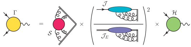
Figure 28: Pictorial representation of soft-collinear factorisation for the quark form factor.

It is important to spend some time on Eq. (4.1), since it forms the basis for further generalisations to fixed-angle scattering amplitudes. We begin by noting that the factorisation of collinear effects into jet functions has required the introduction of a vector $n_{i}^{\mu}$ ($i=1,2$) for each hard parton. The introduction of these vectors can be understood in three complementary ways.

• First of all, such vectors are needed in order to ensure gauge invariance of the jet definition, Eq. (4.9). In the absence of the Wilson line, the jet function would transform as the quark field under a gauge transformation. The Wilson line takes this gauge variation at the origin, and transports it out to infinite distance, where it vanishes, since we are working perturbatively and considering only globally trivial gauge fields.

• The one-loop collinear calculation leading to Eq. (3.54) illustrates that the vectors $n_{i}$, de facto, replace the anti-collinear parton. Collinear gluons absorbed at late times (or emitted at early times) are effectively blind to the detailed structure of non-collinear parts of the amplitude, so that those parts can be replaced, at leading-power accuracy, with a Wilson-line absorber. We recall again that it is important in principle to keep $n_{i}^{2}\neq 0$ (a typical choice [283] for the form factor being $n_{1}=\beta_{1}-\beta_{2}=-n_{2}$). This avoids the inclusion of spurious collinear divergences in the jet function, arising from gluon emission from the Wilson line, which are not present in the form factor and would need to be subtracted.

• A third way to understand the $n_{i}$’s is to think of them as factorisation vectors, generalising the idea of a factorisation scale. Since we are trying to distinguish collinear emissions from wide-angle ones, it is perhaps not surprising that one needs to introduce a vector in order to draw a cone around the direction of the emitter, specified by $\beta_{i}$: in this interpretation, one may decide to assign a gluon to the collinear region if, say, $\beta_{i}\cdot k<n_{i}\cdot k$.

The next set of observations on Eqs. (4.8 - 4.1) concerns their functional dependences. The fact that jet functions can depend only on the variable $(p\cdot n)^{2}/(n^{2}\mu^{2})$ (and similarly eikonal jets can only depend on $(\beta\cdot n)^{2}/n^{2}$) stems from their invariance under rescalings of the form $n\to\kappa n$, which is a property of semi-infinite straight Wilson lines stretching along the direction $n$, with $n^{2}\neq 0$. Indeed, a correlator of two Wilson lines, in directions $n_{i}$, $i=1,2$, with $n_{i}^{2}\neq 0$, can only depend on the Minkowskian cusp angle between the two directions, defined in a Lorentz-invariant way by $\gamma_{12}=(n_{1}\cdot n_{2})^{2}/(n_{1}^{2}n_{2}^{2})$. In the case of light-like Wilson lines, such as those appearing in the soft function and in the eikonal jet function, the cusp angles are ill-defined, so that one might expect correlators involving such lines to be just numbers, free of kinematic dependence. As we have seen in Section 2.7, however, this is not the case, since the rescaling symmetry of Wilson lines correlators is broken by the presence of an extra collinear divergence. As a consequence, the soft function for massless partons acquires a dependence on $\beta_{1}\cdot\beta_{2}$, as shown in Eq. (4.8), and the eikonal jets correspondingly acquire a dependence on $(\beta_{i}\cdot n_{i})^{2}/n_{i}^{2}$. It is clear from the outset that this ‘anomalous’ scale dependence must be comparatively simple, since it is entirely associated with the soft-collinear double pole of the form factor. This double singularity is governed by the light-like cusp anomalous dimension, as we will see in Section 4.2.

A consequence of this analysis, which will be crucial in applications to multi-parton amplitudes, is the following. If we can construct quantities where soft-collinear double poles cancel, then, for these quantities, the anomalous scale dependence must cancel as well. By inspection of Eq. (4.1), we can readily identify two such quantities.

• The ratio of the partonic jet and the corresponding eikonal jet, ${\cal J}_{i}/{\cal J}_{E,\,i}$, which is responsible for hard-collinear corrections, carrying a single collinear pole per loop. In this case, at least at one loop, it is easy to envisage how the cancellation of the anomalous scale dependence takes place: both jets depend logarithmically on their arguments, and one can use

  $$\log\bigg{(}\frac{(p_{i}\cdot n_{i})^{2}}{n_{i}^{2}\mu^{2}}\bigg{)}-\log\bigg{(}\frac{(\beta_{i}\cdot n_{i})^{2}}{n_{i}^{2}}\bigg{)}\,\sim\,\log\bigg{(}\frac{Q^{2}}{\mu^{2}}\bigg{)}\,,$$ (4.13)

  as the two logarithms must have the same coefficient, which stems from the soft-collinear double pole. Explicit expressions for the quark jet and eikonal jet, at one loop, verifying Eq. (4.13), are given in Ref. [70].

• Less trivially, one can define a reduced soft function, by taking the ratio of the soft function with the product of the two eikonal jets,

  $$\widehat{\cal S}\,\big{(}\rho_{12},\alpha_{s}(\mu^{2}),\epsilon\big{)}\,\equiv\,\frac{{\cal S}\Big{(}\beta_{1}\cdot\beta_{2},\alpha_{s}(\mu^{2}),\epsilon\Big{)}}{{\cal J}_{E,\,1}\!\left(\frac{(\beta_{1}\cdot n_{1})^{2}}{n_{1}^{2}},\alpha_{s}(\mu^{2}),\epsilon\right)\,{\cal J}_{E,\,2}\!\left(\frac{(\beta_{2}\cdot n_{2})^{2}}{n_{2}^{2}},\alpha_{s}(\mu^{2}),\epsilon\right)}\,,$$ (4.14)

  which describes soft radiation at wide angles with respect to the hard partons. Also this quantity provides a single (soft) pole per loop, and therefore must be rescaling invariant under $\beta_{i}\to\kappa_{i}\beta_{i}$. This is achieved if $\widehat{\cal S}$ is a function of an invariant variable, which we take here to be

  $$\rho_{12}\,\equiv\,\frac{\big{(}\beta_{1}\cdot\beta_{2}\big{)}^{2}\,n_{1}^{2}\,n_{2}^{2}}{\big{(}\beta_{1}\cdot n_{1}\big{)}^{2}\big{(}\beta_{2}\cdot n_{2}\big{)}^{2}}\,.$$ (4.15)

  Once again, this happens naturally if the dependence of each function in the ratio (4.14) is simply logarithmic, and the logarithms have the same coefficients, tied to the soft-collinear double pole. Clearly, the cancellation implied in Eq. (4.14) is more intricate than the jet case: imposing this constraint will have highly non-trivial consequences in the case of multi-parton amplitudes.

To conclude our analysis of Eq. (4.1), we note the mechanism of cancellation for the dependence on the factorisation vectors $n_{i}$: poles in $\epsilon$ carrying $n_{i}$ dependence must cancel between the partonic and the eikonal jet, through a mechanism akin to Eq. (4.13). On the other hand the hard function ${\cal H}$, which is finite as $\epsilon\to 0$, must depend on $p_{i}\cdot n_{i}$ (or equivalently $\beta_{i}\cdot n_{i}$) in order to cancel the same dependence in the finite parts of the jet functions.

4.2 Evolution and resummation of infrared poles

Based on the discussion at the beginning of the present Section, we expect the soft-collinear factorisation displayed in Eq. (4.1) to lead to an evolution equation, and thus to a resummation, in this case of infrared poles in dimensional regularisation. The basic observation is that, in order to achieve that double factorisation into hard, soft and collinear factors, it was necessary to introduce a factorisation scale separating soft and hard momenta (which we can take equal to the renormalisation scale), and also to introduce the ‘factorisation vectors’ $n_{i}$, separating collinear from wide-angle radiation. Needless to say, the full form factor does not depend on any of these quantities, a statement which directly leads to two evolution equations, which can then be fruitfully combined.

Beginning with the factorisation/renormalisation scale dependence, the fact that we are considering a matrix element of a conserved current leads directly to the RG equation

$$\mu\,\frac{d}{d\mu}\,\Gamma\bigg{(}\frac{Q^{2}}{\mu^{2}},\alpha_{s}(\mu^{2}),\epsilon\bigg{)}\,=\,0\,.$$ (4.16)

If we now rewrite Eq. (4.1) as

$$\Gamma\bigg{(}\frac{Q^{2}}{\mu^{2}}\bigg{)}\,=\,\widehat{\cal S}\big{(}\rho_{12}\big{)}\,{\cal J}_{1}\bigg{(}\frac{(p_{1}\cdot n_{1})^{2}}{n_{1}^{2}\mu^{2}}\bigg{)}\,{\cal J}_{2}\bigg{(}\frac{(p_{2}\cdot n_{2})^{2}}{n_{2}^{2}\mu^{2}}\bigg{)}\,{\cal H}\bigg{(}\frac{Q^{2}}{\mu^{2}},\frac{(p_{i}\cdot n_{i})^{2}}{n_{i}^{2}\mu^{2}}\bigg{)}\,,$$ (4.17)

where we omitted the dependence on the coupling and on $\epsilon$ for brevity, we can define three anomalous dimensions for ${\cal J}_{i}$, $\widehat{\cal S}$, and ${\cal H}$, by taking logarithmic derivatives with respect to the scale, as

$$\mu\frac{d}{d\mu}\ln{\cal J} = -\,\gamma_{\cal J}(\alpha_{s})\,,$$

$$\mu\frac{d}{d\mu}\ln\widehat{\cal S} = -\,\gamma_{\widehat{\cal S}}\left(\rho_{12},\alpha_{s}\right)\,,$$ (4.18)

$$\mu\frac{d}{d\mu}\ln{\cal H} = -\,\gamma_{\cal H}\left(\rho_{12},\alpha_{s}\right)\,.$$

Note that all anomalous dimensions are finite, since the functions we are differentiating have a single pole per loop. Furthermore, note that the jet anomalous dimension $\gamma_{\cal J}$ depends only on the coupling: the partonic jet Eq. (4.9) is not scale-less, therefore UV poles have no direct relation to IR poles, and the anomalous dimension is given by the coefficient of the pole in the UV counterterm; on the other hand, the anomalous dimension for the reduced soft function has a residual kinematic dependence, since, for scale-less quantities, UV singularities are strictly related to IR ones: in this case, there is dependence on the rescaling-invariant variable $\rho_{12}$, leftover after the cancellation of soft-collinear double poles. Finally, the renormalisation group equation (4.16) implies

$$\gamma_{\widehat{\cal S}}\left(\rho_{12},\alpha_{s}\right)+\gamma_{\cal H}\left(\rho_{12},\alpha_{s}\right)+2\gamma_{\cal J}(\alpha_{s})\,=\,0\,;$$ (4.19)

in particular, since $\gamma_{\cal J}$ is independent of $\rho_{12}$, the residual kinematic dependence must cancel between $\gamma_{\cal H}$ and $\gamma_{\widehat{\cal S}}$.

Turning now to the dependence on the factorisation vectors $n_{i}$, first of all we note that this dependence is always through the scalar variables $x_{i}=\left(\beta_{i}\cdot n_{i}\right)^{2}/n_{i}^{2}$ (recall that $p_{i}=\mu\beta_{i}$). Since the complete form factor does not depend on $n_{i}$, we can write

$$x_{i}\frac{\partial}{\partial x_{i}}\ln\Gamma\bigg{(}\frac{Q^{2}}{\mu^{2}},\alpha_{s}(\mu^{2}),\epsilon\bigg{)}\,=\,0\,,$$ (4.20)

where we let the derivative act on the logarithm of the form factor in order to turn the factorisation in Eq. (4.1) into a sum of terms. Taking into account the fact that the soft function does not depend upon $n_{i}$, we find that

$$x_{i}\frac{\partial}{\partial x_{i}}\ln{\cal J}_{i}\,=\,-\frac{1}{2}\,x_{i}\frac{\partial}{\partial x_{i}}\ln{\cal H}+x_{i}\frac{\partial}{\partial x_{i}}\ln{\cal J}_{E,i}\,.$$ (4.21)

Eq. (4.21) is very important, because it achieves the separation of a complicated problem into two simpler ones. The first term on the r.h.s. of Eq. (4.21) can be intricate at high orders, since ${\cal H}$ is a matching function, and thus inherits some of the complexity of the full amplitude: on the other hand, ${\cal H}$ is finite as $\epsilon\to 0$, so the same must be true for its derivative in Eq. (4.21). The second term on the r.h.s. of Eq. (4.21), on the contrary, is divergent as $\epsilon\to 0$ (indeed, it contains only poles in $\epsilon$, since ${\cal J}$ is a pure counterterm in dimensional regularisation); however, its functional form must be extremely simple: indeed, ${\cal J}$ would be just a number, with no kinematic dependence whatsoever, were it not for the anomalous breaking of rescaling invariance due to the collinear poles associated with the $\beta$ direction. Order by order in perturbation theory, these soft-collinear poles are determined by the cusp anomalous dimension, and the ensuing kinematic dependence must be single-logarithmic. It follows that the logarithmic derivative of the eikonal jet ${\cal J}_{i}$ in Eq. (4.21) must be independent of the kinematic variable $x_{i}$. These considerations can be made explicit by defining two functions, corresponding to the two terms on the r.h.s. of Eq. (4.21). For the eikonal jet we define

$$x_{i}\frac{\partial}{\partial x_{i}}\,\ln{\cal J}_{E,i}\,=\,\frac{1}{2}\,\mathcal{K}\Big{(}\alpha_{s}(\mu^{2}),\epsilon\Big{)}\,,$$ (4.22)

while for the hard matching function ${\cal H}$ we define

$$x_{i}\frac{\partial}{\partial x_{i}}\,\ln{\cal H}\,=\,-\,{\cal G}_{i}\Big{(}x_{i},\alpha_{s}(\mu^{2}),\epsilon\Big{)}\,.$$ (4.23)

Eq. (4.21) can then be written as

$$x_{i}\frac{\partial}{\partial x_{i}}\,\ln{\cal J}_{i}\,=\,\frac{1}{2}\,\bigg{[}\,\mathcal{K}\Big{(}\alpha_{s}(\mu^{2}),\epsilon\Big{)}\,+\,{\cal G}_{i}\Big{(}x_{i},\alpha_{s}(\mu^{2}),\epsilon\Big{)}\bigg{]}\,,$$ (4.24)

Eq. (4.24) is an example of a class of equations associated with the soft-collinear evolution of cross-sections and amplitudes in QCD, which we will call ‘Collins-Soper equations’ as they were first derived in Ref. [330]; they were later widely used for resummations of Sudakov logarithms and infrared singularities (see, for example, [226, 283, 293, 331, 332, 70]). In this form, Eq. (4.24) appears rather uninteresting, describing evolution with respect to an unphysical quantity. As is typically the case for RG equations, however, Eq. (4.24), when combined with Eq. (4.16), leads directly to a much more powerful and interesting equation for the evolution of the full form factor with respect to the physical scale $Q^{2}$. Indeed, we can write

$$Q^{2}\frac{\partial}{\partial Q^{2}}\,\ln\Gamma\bigg{(}\frac{Q^{2}}{\mu^{2}},\alpha_{s}(\mu^{2}),\epsilon\bigg{)} = Q^{2}\frac{\partial}{\partial Q^{2}}\,\ln{\cal H}\,+\,\sum_{i=1}^{2}Q^{2}\frac{\partial}{\partial Q^{2}}\,\ln{\cal J}_{i}$$ (4.25)

$$= -\,\mu^{2}\frac{\partial}{\partial\mu^{2}}\,\ln{\cal H}\,+\,\sum_{i=1}^{2}x_{i}\frac{\partial}{\partial x_{i}}\,\ln{\cal J}_{i}\,,$$

where in the first line we have used the fact that purely eikonal functions do not depend on the scale $Q^{2}$, and in the second line we used dimensional analysis, and the fact that jets depend on $Q^{2}$ only through $(p\cdot n)^{2}$. Now for the $\mu$ dependence of the hard function we can use Eq. (4.2) and Eq. (4.19), with the result

$$-\,\mu^{2}\frac{\partial}{\partial\mu^{2}}\,\ln{\cal H} = -\frac{1}{2}\mu\frac{d}{d\mu}\,\ln{\cal H}\,+\,\frac{1}{2}\beta(\epsilon,\alpha_{s})\frac{d}{d\alpha_{s}}\ln{\cal H}$$ (4.26)

$$= \frac{1}{2}\beta(\epsilon,\alpha_{s})\frac{d}{d\alpha_{s}}\ln{\cal H}-\frac{1}{2}\gamma_{\widehat{\cal S}}-\gamma_{\cal J}\,,$$

while Eq. (4.24) gives the $x_{i}$ dependence of the jets. The results can be summarised in a new, much more powerful Collins-Soper equation for the full form factor

$$Q^{2}\frac{\partial}{\partial Q^{2}}\,\ln\Gamma\bigg{(}\frac{Q^{2}}{\mu^{2}},\alpha_{s}(\mu^{2}),\epsilon\bigg{)}\,=\,\frac{1}{2}\,\bigg{[}\,K\Big{(}\alpha_{s}(\mu^{2}),\epsilon\Big{)}\,+\,G\bigg{(}\frac{Q^{2}}{\mu^{2}},\alpha_{s}(\mu^{2}),\epsilon\bigg{)}\bigg{]}\,,$$ (4.27)

where we defined

$$K\Big{(}\alpha_{s}(\mu^{2}),\epsilon\Big{)} \equiv 2{\cal K}\Big{(}\alpha_{s}(\mu^{2}),\epsilon\Big{)}\,,$$

$$G\bigg{(}\frac{Q^{2}}{\mu^{2}},\alpha_{s}(\mu^{2}),\epsilon\bigg{)} \equiv \beta(\epsilon,\alpha_{s})\frac{d}{d\alpha_{s}}\ln{\cal H}-\gamma_{\cal S}-2\gamma_{\cal J}+\frac{1}{2}\sum_{i=1}^{2}{\cal G}_{i}\Big{(}x_{i},\alpha_{s}(\mu^{2}),\epsilon\Big{)}\,.$$ (4.28)

Once again, $K$ is a pure counterterm, and independent of kinematics, while $G$ retains kinematic information, but is finite as $\epsilon\to 0$. There is a final nugget of information to be extracted from Eq. (4.16): since the form factor is not affected by an overall renormalisation, the functions $K$ and $G$ can renormalise additively, but their renormalisations must cancel. Thus

$$\mu\frac{d}{d\mu}\,G\bigg{(}\frac{Q^{2}}{\mu^{2}},\alpha_{s}(\mu^{2}),\epsilon\bigg{)} = -\,\mu\frac{d}{d\mu}\,K\Big{(}\alpha_{s}(\mu^{2}),\epsilon\Big{)}$$ (4.29)

$$= -\,\beta(\epsilon,\alpha_{s})\,\frac{d}{d\alpha_{s}}K\Big{(}\alpha_{s}(\mu^{2}),\epsilon\Big{)}\,\equiv\,\gamma_{K}\big{(}\alpha_{s}(\mu^{2})\big{)}\,,$$

where in the second line we used the fact that $K$ has no explicit scale dependence.

For the purposes of our review, Eq. (4.29) can be taken as an operational definition of the light-like cusp anomalous dimension $\gamma_{K}(\alpha_{s})$. This is, however, such an important object for infrared studies of perturbative gauge theories that it deserves a brief dedicated discussion, before we continue with our analysis of the exponentiation of the form factor.

The function $\gamma_{K}(\alpha_{s})$ appears in several cornerstone gauge-theory calculations. As shown in Ref. [333], it gives the coefficient of the soft singularity of DGLAP splitting functions (discussed here in Section 2.8 and later in Section 6) as the collinear momentum fraction $z\to 1$, to all orders in perturbation theory. As a consequence, it resums leading threshold logarithms in many crucial hadronic cross sections (see, for example, [226, 334, 335, 336]): in that context, it is often denoted by $A(\alpha_{s})$. A closely related function appears in the resummation of leading transverse momentum logarithms in the hadronic production of colour-singlet final states [337, 338], however the two functions begin to differ at the three-loop order [339]. Finally, $\gamma_{K}(\alpha_{s})$ plays a crucial role for Regge behaviour in the high-energy limit [340, 341, 342, 343, 344], and of course, as we discuss below, for the all-order structure of infrared divergences in gauge-theory amplitudes.

The reason for the ubiquitous and crucial role played by the cusp anomalous dimension is not difficult to understand, and emerges from our discussion in Section 3.3.2. In the soft approximation, hard emitters can be replaced by Wilson lines directed along their classical trajectories; then, by the mechanism discussed here in Section 2.7, infrared poles of the original amplitude can be replaced by ultraviolet poles of the corresponding Wilson-line correlator [243]; such correlators (up to collinear divergences) are multiplicatively renormalisable [345, 346, 347, 348]; finally, one finds that the anomalous dimension controlling the ultraviolet divergences arising when two light-like Wilson lines meet at a cusp is given precisely by $\gamma_{K}(\alpha_{s})$. More generally, as noted above in Section 4.1, when two straight Wilson lines directed along non-light-like directions $n_{1}^{\mu}$ and $n_{2}^{\mu}$ meet, forming a Minkowskian angle given by $\gamma_{12}=(n_{1}\cdot n_{2})^{2}/(n_{1}^{2}n_{2}^{2})$, the ultraviolet divergences of the corresponding correlator are controlled by a function $\Gamma_{\rm cusp}(\gamma_{12},\alpha_{s})$, sometimes called angle-dependent cusp anomalous dimension [349]. Not surprisingly, this function plays an essential role for the infrared behaviour of scattering amplitudes and form factors involving massive particles [350, 351, 352, 353]. To all orders, the function $\Gamma_{\rm cusp}(\gamma_{12},\alpha_{s})$ displays a collinear singularity as $n_{i}^{2}\to 0$, or $\gamma_{12}\to\infty$, diverging as the logarithm of $\gamma_{12}$. The coefficient of this logarithm gives the light-like anomalous dimension $\gamma_{K}(\alpha_{s})$.

Quite naturally, perturbative calculations of these vital anomalous dimensions have been the focus of intense activity in the past decades. The light-like cusp anomalous dimension can be extracted from calculations of collinear splitting kernels, so the two-loop result can be traced to Ref. [354], and, in the context of resummation, to Ref. [355]; similarly, the three-loop result emerges from Ref. [356] (see also [357]). At four loops, the result has been computed directly from correlation functions with lagrangian insertions in Ref. [230], and extracted from form factor calculations in Ref. [231]. The full angle-dependent cusp anomalous dimension was computed at two loops in Ref. [244] (see also [358]), and at three loops in Refs. [359, 360]. At four loops, efforts are ongoing, and a wealth of partial information is already available [361, 362, 363, 364, 365]. Perhaps most remarkably, in the special case of ${\cal N}=4$ Super-Yang-Mills theory, the integrability of the planar limit gives access to fully non-perturbative information: gluon amplitudes can be studied in the strong-coupling regime [366], the light-like cusp anomalous dimension can be defined [367], and it can be shown that it obeys a non-perturbative equation [368], which can be analysed both at weak [369, 370, 371] and at strong coupling [372, 373]. We will further discuss the remarkable role played by the cusp for the infrared limit of gauge theory amplitudes in Section 5, where we will also perform in detail the one-loop, angle-dependent calculation.

Returning now to the form factor problem, we note that Eq. (4.29) can be readily solved for $K$, with the result

$$K\Big{(}\alpha_{s}(\mu^{2}),\epsilon\Big{)}\,=\,-\frac{1}{4}\int_{0}^{\mu^{2}}\frac{d\lambda^{2}}{\lambda^{2}}\,\gamma_{K}\big{(}\overline{\alpha}(\lambda^{2},\epsilon)\big{)}\,.$$ (4.30)

Alternatively, it is possible to proceed order by order in perturbation theory, and recursively determine the perturbative coefficients of $K$ in terms of those of the $\beta$ function and of the cusp anomalous dimension $\gamma_{K}$, as was done in Ref. [69]. Up to three loops, the result takes the form

$$K(\alpha_{s},\epsilon) = \frac{\alpha_{s}}{\pi}\,\frac{\gamma_{K}^{(1)}}{4\epsilon}\,+\left(\frac{\alpha_{s}}{\pi}\right)^{2}\,\left(\frac{\gamma_{K}^{(2)}}{8\epsilon}-\frac{b_{0}\,\gamma_{K}^{(1)}}{32\epsilon^{2}}\right)$$ (4.31)

$$\,+\left(\frac{\alpha_{s}}{\pi}\right)^{3}\left(\frac{\gamma_{K}^{(3)}}{12\epsilon}-\frac{b_{0}\,\gamma_{K}^{(2)}+b_{1}\,\gamma_{K}^{(1)}}{48\epsilon^{2}}+\frac{b_{0}^{2}\,\gamma_{K}^{(1)}}{192\epsilon^{3}}\right)\,+{\cal O}(\alpha_{s}^{4})\,.$$

The function $K$ has a long history in the context of perturbative QCD (see, for example, Ref. [330]), and plays an important role also for multi-particle scattering amplitudes, and in the high-energy limit, as we will see in Section 5.

Solving Eq. (4.27) is a standard exercise, but in this case the consistent use of dimensional regularisation yields a very significant simplification: indeed, working with $\epsilon<0$, one can use the fact that the $d$-dimensional strong coupling vanishes in the infrared to impose the simple boundary condition

$$\Gamma\Big{(}0,\alpha_{s}(\mu^{2}),\epsilon\Big{)}\,=\,\Gamma\Big{(}1,\overline{\alpha}(0,\epsilon),\epsilon\Big{)}\,=\,1\,,$$ (4.32)

where on the l.h.s we have set $Q^{2}=0$ for fixed $\mu$, while in the second step we have first set $\mu^{2}=Q^{2}$, and then taken $\mu\to 0$. Thanks to Eq. (4.32), the form factor is a pure exponential with no prefactor, and can be written as [68]

$$\Gamma\bigg{(}\frac{Q^{2}}{\mu^{2}},\alpha_{s}(\mu^{2}),\epsilon\bigg{)}\!\! = \!\!\exp\Bigg{[}\frac{1}{2}\int_{0}^{-Q^{2}}\frac{d\xi^{2}}{\xi^{2}}\Bigg{(}K\Big{(}\alpha_{s}(\mu^{2}),\epsilon\Big{)}+G\Big{(}\!-\!1,\overline{\alpha}(\xi^{2},\epsilon),\epsilon\Big{)}$$ (4.33)

$$\hskip 56.9055pt+\,\frac{1}{2}\int_{\xi^{2}}^{\mu^{2}}\frac{d\lambda^{2}}{\lambda^{2}}\,\gamma_{K}\big{(}\overline{\alpha}(\lambda^{2},\epsilon)\big{)}\Bigg{)}\Bigg{]}\,,$$

where we have used Eq. (4.29) to evolve $G$ from the scale $\xi^{2}$ to the scale $\mu^{2}$, and we have chosen to integrate to the scale $(-Q^{2})$ to emphasise that the form factor is real for negative $Q^{2}$: in this way, $G(-1)$ is real, and all phases can be explicitly obtained by analytic continuation. We note that in Eq. (4.33), in its present form, one needs a non-trivial cancellation of ill-defined contributions between the first term, which diverges at the lower limit of integration, since $K$ does not depend on $\xi$, and the contribution of the upper limit of integration of the $\lambda$ integral, which also does not depend on $\xi$. This cancellation can be performed analytically by using Eq. (4.30), which easily leads to the final expression for the form factor,

$$\Gamma\bigg{(}\frac{Q^{2}}{\mu^{2}},\alpha_{s}(\mu^{2}),\epsilon\bigg{)}\!\!\!\! = \!\!\!\!\exp\Bigg{[}\frac{1}{2}\int_{0}^{-Q^{2}}\frac{d\xi^{2}}{\xi^{2}}\Bigg{(}\!G\Big{(}\!-\!1,\overline{\alpha}(\xi^{2},\epsilon),\epsilon\Big{)}-\frac{1}{2}\,\gamma_{K}\big{(}\overline{\alpha}(\xi^{2},\epsilon)\big{)}\ln\!\bigg{(}\frac{-Q^{2}}{\xi^{2}}\bigg{)}\!\!\Bigg{)}\Bigg{]}\!.$$ (4.34)

As promised, all the ingredients entering the exponent in Eq. (4.34) are finite as $\epsilon\to 0$, and all infrared poles, to all orders in perturbation theory, are generated by the scale integration.

It is worthwhile at this point to pause for a few considerations on Eq. (4.34), which is the simplest case of exponentiation of infrared poles for non-abelian scattering amplitudes, anticipating many features that will be generalised to multi-particle amplitudes in Section 5.

• Perhaps the first point to emphasise is the fact that Eq. (4.34) is predictive: we are not simply shifting the problem from the calculation of $\Gamma$ to the calculation of its logarithm. To see this, note that the direct computation of the form factor order by order yields two infrared poles per loop, so that one finds $\epsilon^{-2n}$ poles at ${\cal O}(\alpha_{s}^{n})$. The exponent in Eq. (4.34), on the other hand, has only one infrared pole per loop beyond one loop: the logarithm of the form factor has singularities up to $\epsilon^{-n-1}$ at ${\cal O}(\alpha_{s}^{n})$. Clearly, all poles of the form $\alpha_{s}^{n}\epsilon^{-p}$ with $n+1<p\leq 2n$ are generated at lower orders and can be obtained by exponentiation: for example, the one-loop calculation of the form factor predicts the leading poles to all orders in perturbation theory. One can in fact look at Eq. (4.33) a little closer, and note that a singularity is generated in the exponent by each integration, so that one immediately detects an exponentiated double pole. The remaining poles in the exponent, $\epsilon^{-p}$ with $2<p\leq n+1$, are generated by the running of the the $d$-dimensional coupling: for example, note that the expansion of Eq. (2.27) in powers of $\alpha_{s}(\mu_{0}^{2})$ is finite order by order as $\epsilon\to 0$, but the integration of each term over the scale $\mu$ generates poles proportional to powers of $b_{0}$. Higher-order terms in the $\beta$ function have a similar effect. This predictive structure has been both verified and exploited in finite-order calculations up to four loops [375, 376, 230, 231, 377].

• These considerations lead to a second significant observation: the form factor - perhaps not surprisingly - becomes extremely simple in the case of gauge theories that are conformal in $d=4$, such as ${\cal N}=4$ Super-Yang-Mills theory, and several of its possible deformations. For these theories, the four-dimensional $\beta$ function vanishes to all orders, so that one has

  $$\beta\big{(}\epsilon,\alpha_{s}\big{)}\,=\,-2\epsilon\alpha_{s}\,,$$ (4.35)

  and Eq. (2.28) holds exactly. As a consequence, the scale integrals in Eq. (4.33), or equivalently Eq. (4.34), can be performed explicitly. Expanding the cusp anomalous dimension and the the function $G$ as

  $$\gamma_{K}(\alpha_{s})\,=\,\sum_{n=1}^{\infty}\bigg{(}\frac{\alpha_{s}}{\pi}\bigg{)}^{n}\gamma_{K}^{(n)}\,,\qquad G\big{(}-1,\alpha_{s},\epsilon\big{)}\,=\,\sum_{n=1}^{\infty}\bigg{(}\frac{\alpha_{s}}{\pi}\bigg{)}^{n}G^{(n)}(\epsilon)\,,$$ (4.36)

  one readily finds [79]

  $$\ln\Bigg{[}\Gamma\bigg{(}\frac{Q^{2}}{\mu^{2}},\alpha_{s}(\mu^{2}),\epsilon\bigg{)}\Bigg{]}\!\!\! = \!\!\!-\,\frac{1}{2}\sum_{n=1}^{\infty}\bigg{(}\frac{\alpha_{s}(\mu^{2})}{\pi}\bigg{)}^{\!n}\bigg{(}\frac{\mu^{2}}{-Q^{2}}\bigg{)}^{\!n\epsilon}\Bigg{[}\frac{\gamma_{K}^{(n)}}{2\,n^{2}\epsilon^{2}}+\frac{G^{(n)}(\epsilon)}{n\epsilon}\Bigg{]}\,.$$ (4.37)

  Using Eq. (2.28), one easily sees that Eq. (4.37) displays exact RG invariance (it is independent of $\mu$), as expected. Eq. (4.37) has important consequences: indeed, it is sufficient to determine the infrared singularity structure of all scattering amplitudes in ${\cal N}=4$ SYM in the planar limit. This is easily understood by noting that, for planar gluon amplitudes, soft gluons can only connect two external states that are consecutive in the selected cyclic ordering, so that the infrared divergences of the full planar amplitude are just given by a product of (gluon) form factors. This fact was exploited in Ref. [79] to constrain the ‘BDS’ ansatz for $n$-point planar amplitudes in ${\cal N}=4$ SYM, which was later proved to give the exact all-order result for $n=4$ and $n=5$ [378, 379].

• A non-trivial practical feature of Eq. (4.34) is the fact that it can be directly compared to finite-order results obtained evaluating Feynman diagrams in dimensional regularisation. Using different infrared regulators, the exponential containing singular terms is multiplied by an ‘initial condition’ which depends on a factorisation scale, and in general admits its own perturbative expansion. Using Eq. (4.34), on the other hand, a finite-order calculation can directly be compared to the corresponding expansion of the exponential, thus extracting the perturbative coefficients of $\gamma_{K}$ and $G$. Non-singular contributions to the form factor are encoded in ${\cal O}(\epsilon^{p})$ terms of $G$, with $p>0$, and they also ‘exponentiate’, yielding a weak prediction for higher-order finite contributions [225, 226, 233, 234].

• A final feature of Eq. (4.34) which is worth noting is the fact that it allows for a straightforward extraction of the analytic continuation of the form factor from negative values of $Q^{2}$ (where $\Gamma$ is real) to positive ones [68]. Indeed, the dependence on $Q^{2}$ is just in the upper limit of integration, so that the ratio of the time-like form factor to the space-like one is simply given by the exponential of the same integral, stretching from $+Q^{2}$ to $-Q^{2}$. Since at the origin one only finds integrable singularities, one can deform the integration contour to a half-circle of radius $Q^{2}$ in the complex $\xi^{2}$ plane, showing that this ratio is completely dominated by perturbative contributions in asymptotically free theories. Furthermore, one can show [68] that the poles of this ratio can be collected in an overall divergent phase, given by the counterterm function $K$,

  $$\frac{\Gamma\big{(}Q^{2},\alpha_{s}\big{)}}{\Gamma\big{(}\!-\!Q^{2},\alpha_{s}\big{)}}\Bigg{|}_{\rm poles}\,=\,\exp\bigg{[}{\rm i}\,\frac{\pi}{2}\,K\big{(}\alpha_{s}(Q^{2}),\epsilon\big{)}\bigg{]}\,,$$ (4.38)

  so that the modulus of the ratio is finite. This is relevant for phenomenological applications, since the modulus of the ratio (or related quantities) appears in cross-sections for vector boson or Higgs production [225, 226, 233], and ‘resums’ large constants such as the factor of $\pi^{2}$ appearing in Eq. (2.23). In the case of ${\cal N}=4$ SYM, starting from Eq. (4.37), one can also get a strikingly simple and elegant expression for finite terms, which are given by

  $$\left|\frac{\Gamma\big{(}Q^{2},\alpha_{s}\big{)}}{\Gamma\big{(}\!-\!Q^{2},\alpha_{s}\big{)}}\right|^{2}\,=\,\exp\bigg{[}\frac{\pi^{2}}{4}\gamma_{K}(\alpha_{s})\bigg{]}\,.$$ (4.39)

  Note that the r.h.s. is independent of $Q^{2}$, as expected for a four-dimensional quantity in a conformal theory. Since all quantities in Eq. (4.39) are well-defined at the non-perturbative level, and since the r.h.s. provides a finite, unambiguous resummation of perturbation theory, Eq. (4.39) can be argued to be an exact non-perturbative result. In some cases, such non-perturbative results can be tested against strong-coupling calculations based on the AdS/CFT correspondence [366, 367, 380].

Having completed our survey of the exponentiation of form factors, we now move on to discuss the general case of fixed-angle scattering amplitudes.

5 Fixed-angle scattering amplitudes

We consider now the case of multi-particle, fixed-angle scattering amplitudes in a general massless gauge theory. We write such amplitudes as

$${\cal A}_{n}^{\,a_{1}\ldots a_{n}}\left(\frac{p_{i}}{\mu},\alpha_{s}(\mu^{2}),\epsilon\right)\,,$$ (5.1)

implying that the normalisation has been chosen in order to work with a dimensionless quantity. The spin structure is understood, but we are displaying the colour indices, which in general can belong to different representations of the gauge group. The fixed-angle assumption amounts to the statement that all Mandelstam invariants $s_{ij}=2p_{i}\cdot p_{j}$ are parametrically of the same size, say $\left|s_{ij}\right|\sim Q^{2}$, $\forall\,i,j$. This means that there are no strong scale hierarchies: the cases in which some momentum $p_{i}$ becomes soft, or two momenta $p_{i}$ and $p_{j}$ become collinear, must be treated separately.

For amplitudes in this class, it is not too difficult to generalise the reasoning leading to the soft-collinear factorisation of the form factor, Eq. (4.1). A diagrammatic analysis, using the Landau equations and the Coleman-Norton physical picture, confirms that non-integrable singularities arise only from soft and collinear configurations; soft gluons, and separately collinear gluons, factorise from the hard part by the same reasoning that was applied to the form factor; finally, so long as external particles are not collinear to each other, the factorisation of soft gluons from each jet at leading power is supported by the same diagrammatic arguments and Ward identities. From a physical point of view, at leading power, jets moving in different directions can interact only at the hard scattering, and soft particles cannot resolve either the details of the hard interaction, or the fine structure of streams of massless particles moving collinearly. The most delicate issue in this generalisation is whether different loop momentum regions, other than soft or collinear, could give raise to singularities. Specifically, recall that the soft region for loop momentum $k$ is defined by the scaling

$$k^{\mu}\,=\,\{k^{+},k^{-},{\bf k}_{\perp}\}\,\quad\to\quad\lambda k^{\mu}\,,\qquad\lambda\to 0\,.$$ (5.2)

In the case of collinear scaling, we can separately consider each hard particle in the amplitude, and in each case define the collinear direction as one of the two directions spanning the light-cone: for example, for a given loop momentum $k$, when considering the collinear region $k^{\mu}\parallel p_{i}^{\mu}$, we can choose a frame where $p_{i}^{\mu}=\{p_{i}^{+},0^{-},{\bf 0}_{\perp}\}$; then the collinear scaling is

$$k^{\mu}\,=\,\{k^{+},k^{-},{\bf k}_{\perp}\}\,\quad\to\quad\{k^{+},\lambda k^{-},\sqrt{\lambda}{\bf k}_{\perp}\}\,,\qquad\lambda\to 0\,,$$ (5.3)

which leads to $k^{2}=2k^{+}k^{-}-{\bf k}_{\perp}^{2}$ vanishing uniformly as $\lambda$. One must wonder whether different momentum scalings could lead to singular contributions: a notable possibility is given by soft wide-angle gluons, scaling as

$$k^{\mu}\,=\,\{k^{+},k^{-},{\bf k}_{\perp}\}\,,\quad\to\quad\{\lambda^{p}k^{+},\lambda^{p}k^{-},\lambda{\bf k}_{\perp}\}\,,\quad p\geq 2\,,\qquad\lambda\to 0\,,$$ (5.4)

with respect to one of the hard parton directions. For fixed-angle amplitudes, such gluons essentially have vanishing longitudinal components, and are usually called Glauber gluons. Glauber gluons are known to give important contributions at cross-section level, and the cancellation of the corresponding divergences is a crucial step in the proof of collinear factorisation for collider processes [205, 206]; furthermore, they can contribute to infrared poles of scattering amplitudes when the external particles are allowed to become collinear, while some of the Mandelstam invariants become space-like [207]. For fixed-angle scattering amplitudes, however, Glauber gluons do not contribute at leading power [276].

With these premises, it is easy to propose a generalisation of Eq. (4.1) for multi-particle amplitudes. First of all, we expect that collinear dynamics will be captured by jet functions, which are essentially single-particle quantities, and thus cannot change the colour content of the outgoing state; soft gluons, on the other hand, can connect any pair of hard particles, and they will change the colour of those particles even if they carry a vanishing energy. We expect then that the soft function in Eq. (4.1) will need to be promoted to a colour operator acting on the colour indices of all external particles. The emergent form of soft-collinear factorisation for fixed-angle multi-particle scattering amplitudes in massless gauge theories is then

$${\cal A}_{n}\left(\frac{p_{i}}{\mu},\alpha_{s}(\mu),\epsilon\right) = \prod_{i=1}^{n}\frac{{\cal J}_{i}\left(\frac{\left(p_{i}\cdot n_{i}\right)^{2}}{n_{i}^{2}\mu^{2}},\alpha_{s}(\mu^{2}),\epsilon\right)}{{\cal J}_{E,i}\left(\frac{\left(\beta_{i}\cdot n_{i}\right)^{2}}{n_{i}^{2}},\alpha_{s}(\mu^{2}),\epsilon\right)}$$ (5.5)

$$\times\,{\cal S}_{n}\big{(}\beta_{i}\cdot\beta_{j},\alpha_{s}(\mu^{2}),\epsilon\big{)}\,{\cal H}_{n}\!\left(\!\frac{p_{i}\cdot p_{j}}{\mu^{2}},\frac{\left(p_{i}\cdot n_{i}\right)^{2}}{n_{i}^{2}\mu^{2}},\alpha_{s}(\mu^{2}),\epsilon\right)\,,$$

where we introduced a jet function, and its eikonal counterpart, for each external hard particle, with the definitions given in Eq. (4.9) and Eq. (4.11), and we defined the $n$-particle soft function as the natural generalisation of Eq. (4.8),

$${\cal S}\left(\beta_{i}\cdot\beta_{j},\alpha_{s}(\mu^{2}),\epsilon\right)\,\equiv\,\langle 0|\,T\bigg{[}\prod_{k=1}^{n}\Phi_{\beta_{k}}(\infty,0)\bigg{]}|0\rangle\,.$$ (5.6)

The factorisation in Eq. (5.5) is supported by the exhaustive diagrammatic analysis carried out in Ref. [381], which leads to a BPHZ-like forest formula for soft and collinear singularities in fixed-angle scattering amplitudes. This analysis makes use of the coordinate-space formalism developed in Ref. [224], and generalises the early results of [330, 66]. An independent derivation of an analogous factorisation in the context of SCET was given in [95].

In order to proceed to a more detailed analysis of the factorisation, we first need to be much more concrete concerning the treatment of colour flow in Eq. (5.5), clarifying the action of the soft colour operator ${\cal S}$ on the hard part of the amplitude, ${\cal H}$: this was trivial for form factors, where particles with opposite colour charges annihilate into a colour-singlet state, but can be very intricate for general scattering amplitudes. With this in mind, before proceeding to discuss the dynamical aspects of the soft-collinear factorisation in Eq. (5.5), we briefly digress to describe the two main methods commonly used to handle colour in this general case.

5.1 Handling color structures

The colour structure of a generic multi-particle non-abelian scattering amplitude is an interesting group theory problem, solved in principle with standard tools, but not easy to implement in practice when the particle number grows. In general, each color index in Eq. (5.1) can belong to a different representation of the gauge group $r_{i}$, $i=1,\ldots,n$. The amplitude ${\cal A}$ is a tensor in the vector space ${\cal V}_{n}\equiv r_{1}\otimes\ldots\otimes r_{n}$, and colour conservation implies that it must be an invariant tensor. The task is then to decompose the reducible representation ${\cal V}_{n}$ into a sum of irreducible representations, and impose the colour-conservation constraint on the result. A practical way to do this is to pick a channel, i.e. a set of particles taken as ‘incoming’, and build the tensor product of the corresponding representations; one then repeats the construction for the remaining, ‘outgoing’, particles, and selects the irreducible representations that appear in both lists: those are the possible colour states that can be exchanged in that channel. A thorough analysis of this construction was performed in Ref. [382] (see also [343]): using Clebsch-Gordan coefficients, one can construct projection operators identifying each possible colour flow in the selected channel.

In the present context, our concern is to understand how the colour structure is implemented in the soft-collinear factorisation of the amplitude, Eq. (5.5). In order to represent the action of the soft operator ${\cal S}_{n}$ on the hard matching coefficient ${\cal H}_{n}$, two formalisms are commonly adopted, one based upon a choice of basis in the space of colour tensors available for the selected process, and one formulated in terms of basis-independent colour insertion operators. For completeness, we briefly present below the basics of both formalisms.

5.1.1 Colour tensor bases

Using the techniques discussed in Refs. [382, 343], it is possible to identify, in any selected channel, a basis of colour tensors spanning the representations that can be exchanged in that channel. Denoting the basis tensors by $c_{L}^{\,\,a_{1}\ldots a_{n}}$, we can then write the amplitude as

$${\cal A}_{n}^{\,a_{1}\ldots a_{n}}\left(\frac{p_{i}}{\mu},\alpha_{s}(\mu^{2}),\epsilon\right)\,=\,\sum_{L}{\cal A}_{n}^{L}\left(\frac{p_{i}}{\mu},\alpha_{s}(\mu^{2}),\epsilon\right)\,c_{L}^{\,\,a_{1}\ldots a_{n}}\,.$$ (5.7)

The tensors $c_{L}^{\,\,a_{1}\ldots a_{n}}$ are quadratic combinations of the Clebsch-Gordan coefficients appearing in the decomposition of ${\cal V}_{n}$ in a direct sum of irreducible representations. They can be chosen to be orthonormal, in the sense that

$$\sum_{\{a_{i}\}}c_{L}^{\,\,a_{1}\ldots a_{n}}\,\left(c_{M}^{\,\,a_{1}\ldots a_{n}}\right)^{*}\,=\,\delta_{LM}\,.$$ (5.8)

To illustrate this, consider the simple case of $q\bar{q}$ scattering: at tree level, the contributing diagrams are depicted in Fig. 29. Applying the Feynman rules, and the Fierz identity

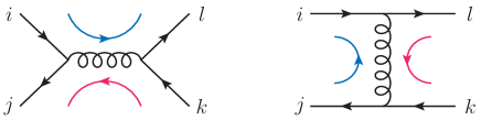
Figure 29: Feynman diagrams for tree-level quark-antiquark scattering, and their colour flow at leading power in $N_{c}$.

$$\big{(}T_{a}\big{)}_{ij}\,\big{(}T^{a}\big{)}_{kl}\,=\,\frac{1}{2}\bigg{(}\delta_{il}\delta_{jk}-\frac{1}{N_{c}}\delta_{ij}\delta_{kl}\bigg{)}\,,$$ (5.9)

one immediately identifies a possible set of basis color tensors as

$$\hat{c}_{1}^{\,ijkl}\,=\,\delta^{il}\delta^{jk}\,,\qquad\hat{c}_{2}^{\,ijkl}\,=\,\delta^{ij}\delta^{kl}\,,$$ (5.10)

corresponding to leading-color flow in the $s$ channel and in the $t$ channel, respectively. It is clear that this set forms a basis for higher-order corrections as well, since the third possible combination of Kronecker $\delta$ functions in the fundamental representation is forbidden, as it would require a quark to turn into an antiquark. More formally, one would start by noting that the representations entering the scattering (for example in the $s$ channel) give $\underline{\bf 3}\otimes\underline{\bf 3}^{*}=\underline{\bf 1}\oplus\underline{\bf 8}$: one then expects a set of only two basis tensors. The correspondence between the basis tensors and the representation content is made more transparent by transforming the basis in Eq. (5.10) to an orthonormal one, according to Eq. (5.8), by using again Eq. (5.9). One can then pick

$$c_{1}^{\,ijkl}\,=\,\frac{2}{\sqrt{N_{c}^{2}-1}}\big{(}T_{a}\big{)}_{ji}\,\big{(}T^{a}\big{)}_{kl}\,,\qquad c_{2}^{\,ijkl}\,=\,\frac{1}{N_{c}}\,\delta^{ij}\delta^{kl}\,,$$ (5.11)

corresponding to octet and singlet $s$-channel exchanges, respectively. Once a basis has been selected, the amplitude can be thought of as a vector in the vector space spanned by the $c_{L}$ tensors. In the chosen basis, the soft operator is represented by a matrix, acting on a vector of hard matching coefficients. To be precise, we note that the Wilson lines in Eq. (5.6) have open colour indices at both ends, and both sets of indices can be projected on the basis tensors. We define then the matrix elements ${\cal S}^{\,\,L}_{n\,\,K}$ of the soft operator, in the chosen basis, by

$$\sum_{L}c_{L}^{\,\,a_{1}\ldots a_{n}}\,{\cal S}^{\,\,L}_{n\,\,K}\big{(}\beta_{i}\cdot\beta_{j},\alpha_{s}(\mu^{2}),\epsilon\big{)}\,=\,\sum_{b_{1},\ldots,b_{n}}\langle 0|\prod_{k=1}^{n}\Big{[}\Phi_{\beta_{k}}(\infty,0)\Big{]}^{a_{k}}_{\,\,\,\,b_{k}}|0\rangle\,c_{K}^{\,\,b_{1}\ldots b_{n}}\,;$$ (5.12)

in Eq. (5.5), the soft matrix thus defined acts on a vector of finite matching coefficients ${\cal H}^{K}$.

Working with explicit colour bases is useful for practical applications, for example for the implementation of soft gluon resummations in hadron scattering [383, 384, 385, 386, 387]. The formalism, however, does not easily lend itself to the general treatment of $n$-point amplitudes: the size of the matrices involved grows steeply with the number of particles, and colour conservation is implemented essentially on a process-by-process basis. For example, the treatment of $gg\to gg$ scattering in $SU(N_{c})$ requires 9$\times$9 matrices (although some simplification are possible [388, 389]), while already for amplitudes involving five gluons ($gg\to ggg$) the matrices involved have dimension $d=44$ [390]. We now proceed to describe a formalism which is better suited for generic particle multiplicities.

5.1.2 Colour insertion operators

Considering soft-gluon corrections, the factorisation formula in Eq. (5.5) formalises an intuitive understanding: soft divergences arise when soft gluons (real or virtual) are emitted from an on-shell particle. Essentially, this means that soft divergences are associated with emissions from external legs, so that one can think of the soft operator as acting ‘from the outside’ on the hard factor, which contains corrections associated with ‘inner’, off-shell virtual exchanges. It then makes sense, at leading power, to think of the soft emission as a colour operator, inserting a soft gluon on the non-radiative amplitude, according to the scheme

$${\cal A}_{n+1}^{\,\,a\,b_{1}\ldots\,b_{n}}\bigg{|}_{\rm soft}\,\propto\,\sum_{i=1}^{n}\Big{[}{\bf T}_{i}^{\,a}\Big{]}^{b_{i}}_{\,\,\,c_{i}}{\cal A}_{n}^{\,\,b_{1}\ldots\,c_{i}\ldots\,b_{n}}\,.$$ (5.13)

The colour operators ${\bf T}_{i}$ act on the tensor product space ${\cal V}_{n}$, and the index $i$ identifies the specific factor in the product on which the operator acts non-trivially, corresponding to the emission of a gluon with (adjoint) index $a$ from particle $i$. In order to be more precise, and to illustrate how this operator formalism emerges [289, 81], consider the case of soft gluon emission from an outgoing quark, in a generic tree-level matrix element involving $n$ coloured particles, plus the emitted gluon. Let the $n$ ‘Born-level’ particles have momenta $p_{i}$, colour indices $c_{i}$ and polarisation $\lambda_{i}$, and let the radiated gluon be characterised by momentum $k$, colour $c$ and polarisation $\lambda$. The only diagrams surviving at leading power in $k$ are those where the soft gluon is emitted by the on-shell external legs, so we can easily isolate the contribution of a specific outgoing quark, say the one carrying momentum $p_{i}$. The relevant contribution to the emission amplitude is given by

$$g\mu^{\epsilon}\,\overline{u}_{s_{i}}(p_{i})\,\gamma_{\alpha}\,\frac{p\hskip-4.49997pt/_{i}+k\hskip-4.49997pt/}{2p_{i}\cdot k}\,\big{(}T^{c}\big{)}_{c_{i}d_{i}}\widehat{\cal A}^{\,\,\,c_{1}\ldots\,d_{i}\ldots\,c_{n}}_{\,s_{1}\dots s_{n}}\big{(}\{p_{j}\},k\big{)}\,\epsilon_{\lambda}^{*\,\alpha}(k)\,,$$ (5.14)

where $\widehat{\cal A}$, while not quite a scattering amplitude itself, since the $i$-th leg is off-shell for generic $k$, represents all the remaining factors of the radiative amplitude. Now, taking the soft limit $k^{\mu}\to 0$, we can apply the eikonal approximation to the factors associated with the $i$-th particle, and, at leading power in $k$, we can neglect $k$ in the factor $\widehat{\cal A}$, which thus becomes precisely the ‘Born’ amplitude for the original $n$ on-shell particles. Following the steps already outlined in Section 1 in the case of QED, this leads to the expression

$$g\mu^{\epsilon}\,\frac{\beta_{i}\cdot\epsilon_{\lambda}^{*}(k)}{\beta_{i}\cdot k}\,\big{(}T^{c}\big{)}_{c_{i}d_{i}}\big{(}{\cal A}_{n}\big{)}^{\,c_{1}\ldots\,d_{i}\ldots\,c_{n}}_{s_{1}\dots s_{n}}\big{(}\{p_{j}\}\big{)}\,\equiv\,g\mu^{\epsilon}\,\frac{\beta_{i}\cdot\epsilon_{\lambda}^{*}(k)}{\beta_{i}\cdot k}\,\,{\bf T}_{i}\,{\cal A}_{n}\big{(}\{p_{j}\}\big{)}\,.$$ (5.15)

We have thus identified the precise expression for the colour operator ${\bf T}_{i}$, when the $i$-th particle is an outgoing quark: in that case, ${\bf T}_{i}$ is the colour generator $T^{a}_{\,\,cd}$, in the fundamental representation. Performing the same calculation for an outgoing antiquark, and an outgoing gluon, one finds the identifications

$${\bf T}_{i}\Big{|}_{\rm q,\,out}\,\to\,T^{a}_{\,\,cd}\,,\qquad{\bf T}_{i}\Big{|}_{\rm\bar{q},\,out}\,\to\,-\,T^{a}_{\,\,dc}\,,\qquad{\bf T}_{i}\Big{|}_{\rm g,\,out}\,\to\,-\,{\rm i}f^{a}_{\,\,cd}\,,$$ (5.16)

with the convention that the colour index $d$ is the one to be contracted with the Born amplitude; the action on incoming particles is defined by crossing symmetry: it is unchanged for gluons, while the expressions for quarks and antiquarks are interchanged. Notice that the negative sign for antiquarks in Eq. (5.16) emerges from the orientation of the fermion line of the Born amplitude, which is opposite to the (outgoing) momentum flow for an antiparticle.

In case the soft gluon is emitted into the final state, this discussion sketches the derivation of the tree-level current for the emission of a soft-gluon with momentum $k$,

$${\bf J}^{\mu}(k)\,=\,g\mu^{\epsilon}\sum_{i=1}^{n}\frac{\beta_{i}^{\mu}}{\beta_{i}\cdot k}\,{\bf T}_{i}\,,$$ (5.17)

which will be discussed in greater detail in Section 6. If the soft gluon is virtual, it will be reabsorbed by another hard particle, leading to the colour-dipole structure ${\bf T}_{i}\cdot{\bf T}_{j}$, where the product implies a sum over the soft gluon colour indices. Since the colour operators ${\bf T}_{i}$ act non-trivially only on the colour index of particle $i$, operators acting on different particles commute, and they satisfy the algebra

$${\bf T}_{i}\cdot{\bf T}_{j}\,=\,{\bf T}_{j}\cdot{\bf T}_{i}\,\qquad(i\neq j)\,;\qquad{\bf T}_{i}\cdot{\bf T}_{i}\,\equiv\,{\bf T}_{i}^{2}\,=\,C^{(2)}_{r_{i}}\,,$$ (5.18)

where $C^{(2)}_{r_{i}}$ is the quadratic Casimir eigenvalue for the representation $r_{i}$, so that $C^{(2)}_{A}\equiv C_{A}=N_{c}$ and $C^{(2)}_{F}\equiv C_{F}=(N_{c}^{2}-1)/2N_{c}$ for the adjoint and the fundamental representations, respectively. The statement that the scattering amplitude is an invariant tensor of the colour group is represented in this formalism by the fact that, when acting on the non-radiative amplitude, the colour operators satisfy

$$\sum_{i=1}^{n}{\bf T}_{i}\,=\,0\,,$$ (5.19)

which, as we will see, poses a non-trivial constraint on the structure of the soft operator at high orders. This brief introduction suggests that the colour operator notation, while somewhat more formal, and thus perhaps less suited to concrete applications, is very powerful to construct general statements about scattering amplitudes with a generic number of particles. In what follows, we will often leave the colour structure implicit, treating the soft matrix as a formal colour operator, as in Eq. (5.5): when needed, we will adapt our notation, either by choosing a basis or by explicitly introducing colour operators.

5.2 The dipole formula and beyond

Having dealt with ways to handle the colour structure of the factorised amplitude, we now turn back to explore the all-important dynamical consequences of the factorisation in Eq. (5.5). As we will see, most of the considerations that were discussed in Section 4.1 in the case of form factors still apply for the general case of fixed-angle amplitudes, but they turn out to have much more powerful consequences.

The first point to notice is that the soft function defined in Eq. (5.6), like its two-line counterpart in Eq. (4.8), obeys a renormalisation group equation, which however now has a matrix form. Technically, multiplicative renormalisability of (straight) Wilson-line correlators holds when the lines are not on the light cone, or in the presence of a collinear regulator: formally, for the moment, we are going to use dimensional regularisation as a collinear regulator, while later, for concrete calculations in Section 5.3, it will turn out to be more practical to tilt Wilson lines off the light cone and reserve dimensional continuation for the control of UV divergences. With this understanding, the renormalisation group equation for the soft operator (in a selected colour basis) reads

$$\mu\frac{d}{d\mu}\,{\cal S}_{LK}\left(\beta_{i}\cdot\beta_{j},\alpha_{s}(\mu^{2}),\epsilon\right)\,=\,-\,{\cal S}_{L}^{\,\,\,M}\left(\beta_{i}\cdot\beta_{j},\alpha_{s}(\mu^{2}),\epsilon\right)\Gamma^{({\cal S})}_{MK}\left(\beta_{i}\cdot\beta_{j},\alpha_{s}(\mu^{2}),\epsilon\right)\,,$$ (5.20)

which defines the anomalous dimension matrix $\Gamma^{({\cal S})}$. At this stage, $\Gamma^{({\cal S})}$ is not finite, but carries collinear poles in $\epsilon$. The solution to Eq. (5.20) can readily be written as

$${\cal S}\left(\beta_{i}\cdot\beta_{j},\alpha_{s}(\mu^{2}),\epsilon\right)\,=\,{\cal P}\exp\left[-\frac{1}{2}\int_{0}^{\mu^{2}}\frac{d\xi^{2}}{\xi^{2}}\,\Gamma^{({\cal S})}\big{(}\beta_{i}\cdot\beta_{j},\alpha_{s}(\xi^{2},\epsilon),\epsilon\big{)}\right]\,,$$ (5.21)

where we used the vanishing of the $d$-dimensional coupling in the infrared, and we have shuffled the tree-level colour structure into the hard coefficient function.

It would be nice, of course, to deal with a finite anomalous dimension matrix, and this is where the full power of the soft-collinear factorisation of the amplitude can be brought to bear. Indeed, as was the case for form factors, we can organise Eq. (5.5) either by building the hard-collinear combinations ${\cal J}_{i}/{\cal J}_{E,i}$, which have no soft poles, or, much more interestingly, by defining the reduced soft matrix

$$\widehat{\cal S}_{LK}\big{(}\rho_{ij},\alpha_{s}(\mu^{2}),\epsilon\big{)}\,\equiv\,\frac{{\cal S}_{LK}\left(\beta_{i}\cdot\beta_{j},\alpha_{s}(\mu^{2}),\epsilon\right)}{\prod_{i=1}^{n}{\cal J}_{E,i}\left(\frac{\left(\beta_{i}\cdot n_{i}\right)^{2}}{n_{i}^{2}},\alpha_{s}(\mu^{2}),\epsilon\right)}\,.$$ (5.22)

which must be free of collinear poles, and is responsible for wide-angle soft singularities. We see, however, that in this case the cancellation is much more surprising, since the numerator of Eq. (5.22) is a matrix, while the denominator is just a number. Clearly, this poses strong constraints on the soft operator: for example, as the notation suggests, the anomalous dependence on the light-like vectors $\beta_{i}$ must cancel along with the collinear poles, which forces the reduced soft function to depend on $n_{i}$ only through the rescaling-invariant ratios introduced in Eq. (4.15),

$$\rho_{ij}\,\equiv\,\frac{\left(\beta_{i}\cdot\beta_{j}\right)^{2}\,n_{i}^{2}\,n_{j}^{2}}{\left(\beta_{i}\cdot n_{i}\right)^{2}\left(\beta_{j}\cdot n_{j}\right)^{2}}\,.$$ (5.23)

The full power of the constraints arising from Eq. (5.22) is best displayed at the level of the anomalous dimensions. One can write the renormalisation group equation for the reduced soft function as

$$\mu\frac{d}{d\mu}\,\widehat{\cal S}_{LK}\left(\rho_{ij},\alpha_{s}(\mu^{2}),\epsilon\right)\,=\,-\,\widehat{\cal S}_{L}^{\,\,\,M}\left(\rho_{ij},\alpha_{s}(\mu^{2}),\epsilon\right)\Gamma^{(\widehat{\cal S})}_{MK}\left(\rho_{ij},\alpha_{s}(\mu^{2})\right)\,,$$ (5.24)

and then note that the matrix $\Gamma^{(\widehat{\cal S})}$ can be written as

$$\Gamma^{(\widehat{\cal S})}_{KL}\left(\rho_{ij},\alpha_{s}(\mu^{2})\right)\,=\,\Gamma^{({\cal S})}_{KL}\left(\beta_{i}\cdot\beta_{j},\alpha_{s}(\mu^{2}),\epsilon\right)-\delta_{KL}\,\sum_{i=1}^{n}\gamma_{{\cal J}_{E}}\!\left(\!\frac{\left(\beta_{i}\cdot n_{i}\right)^{2}}{n_{i}^{2}},\alpha_{s}(\mu^{2}),\epsilon\right)\,,$$ (5.25)

where $\gamma_{{\cal J}_{E}}$ is the anomalous dimension for the eikonal jet function, which carries the anomalous dependence on the jet direction $\beta_{i}$, arising from soft-collinear double poles. It is immediately clear that three separate powerful constraints on the soft anomalous dimension matrix $\Gamma^{({\cal S})}$ arise from Eq. (5.25).

• Collinear poles in $\Gamma^{({\cal S})}$ must be confined to the diagonal entries of the matrix, and they must be determined solely by the light-like cusp anomalous dimension $\gamma_{K}$, which governs soft-collinear singularites, and thus fixes $\gamma_{{\cal J}_{E}}$ [74].

• Finite diagonal terms in $\Gamma^{({\cal S})}$ must combine with finite terms in $\gamma_{{\cal J}_{E}}$ to form the rescaling-invariant ratios $\rho_{ij}$ in Eq. (5.23), as was the case for the form factor.

• Off-diagonal terms in $\Gamma^{({\cal S})}$ must be finite, and furthermore they must, by themselves, be rescaling-invariant functions of the four-velocities $\beta_{i}$. Thus, they can only depend on conformal-invariant cross ratios of the form

  $$\rho_{ijkl}\,=\,\frac{\beta_{i}\cdot\beta_{j}\,\beta_{k}\cdot\beta_{l}}{\beta_{i}\cdot\beta_{k}\,\beta_{j}\cdot\beta_{l}}\,.$$ (5.26)

In order to translate these qualitative statements into a precise mathematical formulation, we can take a derivative of the matrix $\Gamma^{(\widehat{\cal S})}$ with respect the arguments $x_{i}=\left(\beta_{i}\cdot n_{i}\right)^{2}/n_{i}^{2}$, which only occur in the eikonal jets. We find

$$x_{i}\frac{\partial}{\partial x_{i}}\,\Gamma_{KL}^{(\widehat{\cal S})}\left(\rho_{ij},\alpha_{s}\right)\,=\,-\,\delta_{KL}\,\,x_{i}\frac{\partial}{\partial x_{i}}\,\gamma_{J_{E}}\,=\,-\,\frac{1}{4}\,\gamma_{K}(\alpha_{s})\,\delta_{KL}\,,$$ (5.27)

where the last equality expresses the fact that kinematic dependence in the eikonal jets can only arise through the superposition of soft and collinear singularities, and is thus determined by the light-like cusp anomalous dimension $\gamma_{K}(\alpha_{s})$. The precise form of the equality follows from a detailed analysis of the RG equation for the eikonal jet [74], as well as from the general arguments leading to Collins-Soper equations, as first laid out in Ref. [330]. We know, however, that $\Gamma^{(\widehat{\cal S})}$ can only depend on $x_{i}$ through the combinations $\rho_{ij}$ defined in Eq. (5.23). Using the chain rule we then conclude that [74, 75]

$$\sum_{i=1}^{n}\sum_{j\neq i}\,\frac{\partial}{\partial\ln\rho_{ij}}\,\Gamma_{KL}^{(\widehat{\cal S})}\left(\rho_{ij},\alpha_{s}\right)\,=\,\frac{1}{4}\,\gamma_{K}(\alpha_{s})\,\delta_{KL}\,.$$ (5.28)

Eq. (5.28) governs the interplay of colour and kinematics in the soft anomalous dimension matrix to all orders in perturbation theory, and is an exact result.

Our remaining task is now to solve Eq. (5.28). As we are dealing with a linear inhomogeneous partial differential equation, the general solution can be expressed as the sum of a particular solution of the inhomogeneous problem, plus a generic solution of the corresponding homogeneous equation. In order to proceed, we now shift from the basis-dependent notation employed thus far to the colour-operator notation: upon making a single approximation, this will allow us to write a particular solution of Eq. (5.28) in a transparent and elegant way. We begin by noting that the cusp anomalous dimension in colour representation $r$ can be computed from the form factor for particles trasforming under $r$, and admits a Casimir expansion [391, 392, 393, 394]

$$\gamma_{K}^{(r)}(\alpha_{s})\,=\,\sum_{p,i}^{\infty}C^{\,(2p,i)}_{r}\,\,\widehat{\gamma}^{\,(2p,i)}_{K}(\alpha_{s})\,,$$ (5.29)

where $C^{\,(n,i)}_{r}$ are eigenvalues of $n$-th order Casimir operators of the Lie algebra, in representation $r$, and the functions $\widehat{\gamma}^{\,(2p,i)}_{K}$ are independent of $r$. The index $i$ takes into account possible dependence on the matter content of the particular gauge theory under consideration: in ordinary QCD, for example, one finds loop-level contributions involving both the adjoint and the fundamental representations. For $p>1$, building a Casimir invariant of order $2p$ requires $2p$ gluon attachments to the Wilson lines, and a further $2p$ vertices (for example forming a loop) in order to build a symmetric colour tensor saturating the open colour indices. Thus, for example, quartic Casimir contributions (corresponding to $p=2$) will start at four loops, sixth-order Casimir contributions ($p=3$) at six loops, and so on; quadratic Casimirs are special because they are built with the Lie algebra metric tensor $\delta_{ab}$, so that the corresponding contribution starts at one loop. Finite-order calculations indeed confirm that the cusp anomalous dimension obeys Casimir scaling up to three loops (i.e. it is proportional to the quadratic Casimir eigenvalue $C^{(2)}_{r}$), while it develops quartic Casimir components at four loops, as expected [395, 363, 396, 397, 398, 230, 399, 231].

Given this general structure, it is both phenomenologically and theoretically interesting to begin by focusing on the quadratic Casimir component of the cusp, which provides the full answer up to three loops. This component yields a simple solution to Eq. (5.28), since one can write (using Eq. (5.18))

$$\gamma_{K}^{(r)}(\alpha_{s})\,=\,C^{(2)}_{r}\,\widehat{\gamma}_{K}(\alpha_{s})\,=\,\widehat{\gamma}_{K}(\alpha_{s})\,{\bf T}_{i}\cdot{\bf T}_{i}\,,$$ (5.30)

where for simplicity we dropped the Casimir-counting indices in Eq. (5.29). It is then easy to verify, using Eq. (5.19), that the ‘dipole sum’

$$\Gamma_{\rm dip}^{(\widehat{\cal S})}\left(\rho_{ij},\alpha_{s}\right)\,=\,-\,\frac{1}{8}\,\widehat{\gamma}_{K}(\alpha_{s})\sum_{i=1}^{n}\sum_{j\neq i}\ln\rho_{ij}\,{\bf T}_{i}\cdot{\bf T}_{j}\,+\,\delta^{\,(\widehat{\cal S})}(\alpha_{s})\,\sum_{i=1}^{n}{\bf T}_{i}\cdot{\bf T}_{i}\,,$$ (5.31)

is a solution of Eq. (5.28), with the function $\delta^{\,(\widehat{\cal S})}$ playing the role of an integration constant. Before highlighting the important properties of Eq. (5.31), it is useful to embed it in the full factorisation of the amplitude, in order to get rid of the unphysical dependence on the auxiliary vectors $n_{i}$, which still feature in Eq. (5.31) through the variables $\rho_{ij}$. Indeed, as already noted at the end of Section 4.1, $n_{i}$-dependent singular terms must cancel in the ratio of jets and eikonal jets, whereas finite $n_{i}$-dependent terms must cancel between the jets and the hard matching function ${\cal H}$. Performing these cancellations, order by order in perturbation theory, yields a simplified form for the soft-collinear factorisation of fixed-angle amplitudes, which can be written as [75, 76]

$${\cal A}_{n}\left(\frac{p_{i}}{\mu},\alpha_{s}(\mu^{2}),\epsilon\right)\,=\,{\cal Z}_{n}\left(\frac{p_{i}}{\mu},\alpha_{s}(\mu^{2}),\epsilon\right){\cal F}_{n}\left(\frac{p_{i}}{\mu},\alpha_{s}(\mu^{2}),\epsilon\right)\,,$$ (5.32)

where ${\cal Z}_{n}$ is a colour operator generating all infrared singularities, and acting on the finite vector ${\cal F}_{n}$. Since the non-trivial colour structure of ${\cal Z}_{n}$ arises entirely from the soft factor, it will obey a matrix renormalisation group equation of the same form as Eq. (5.24), and the solution will again be an exponential, which we can write as

$${\cal Z}_{n}\left(\frac{p_{i}}{\mu},\alpha_{s}(\mu^{2}),\epsilon\right)\,=\,{\cal P}\exp\left[\frac{1}{2}\int_{0}^{\mu^{2}}\frac{d\lambda^{2}}{\lambda^{2}}\,\,\Gamma_{n}\left(\frac{p_{i}}{\lambda},\alpha_{s}\!\left(\lambda^{2},\epsilon\right)\right)\right]\,,$$ (5.33)

with the full infrared anomalous dimension matrix $\Gamma_{n}$ satisfying a constraint equation inherited from Eq. (5.28). The general solution to that equation will take the form

$$\Gamma_{n}\left(\frac{p_{i}}{\mu},\alpha_{s}(\mu^{2})\right)\,=\,\Gamma_{n}^{\rm dip}\left(\frac{s_{ij}}{\mu^{2}},\alpha_{s}(\mu^{2})\right)\,+\,\Delta_{n}\left(\rho_{ijkl},\alpha_{s}(\mu^{2})\right)\,,$$ (5.34)

with $\Gamma_{n}^{\rm dip}$ a particular solution of the inhomogeneous equation, akin to Eq. (5.31), and $\Delta_{n}$ the general solution of the homogeneous problem. Considering first the dipole term, after the cancellation of of the dependence on the auxiliary vectors, the logarithms of the scaling variables $\rho_{ij}$ must be replaced with logarithms of the corresponding Mandelstam invariants. At this point we can also reinstate the analytic properties, which we have neglected so far, recalling from Section 4.1 that time-like invariants carry imaginary parts. With these considerations, we can finally write the dipole formula as [73, 74, 75, 76]

$$\Gamma_{n}^{\rm dip}\bigg{(}\frac{s_{ij}}{\mu^{2}},\alpha_{s}(\mu^{2})\bigg{)}\,=\,\frac{1}{2}\,\widehat{\gamma}_{K}\left(\alpha_{s}(\mu^{2})\right)\sum_{i=1}^{n}\sum_{j=i+1}^{n}\log\left(\frac{s_{ij}\,{\rm e}^{{\rm i}\pi\lambda_{ij}}}{\mu^{2}}\right){\bf T}_{i}\cdot{\bf T}_{j}+\sum_{i=1}^{n}\gamma_{i}\left(\alpha_{s}(\mu^{2})\right)\,,$$ (5.35)

where $\gamma_{i}$ are colour-diagonal anomalous dimensions arising from jet functions, and the phases are given by $\lambda_{ij}=1$, if particles $i$ and $j$ are either both in the final state or both in the initial state, while $\lambda_{ij}=0$ otherwise.

Turning now to the homogeneous problem, we note that the operator $\Delta_{n}$, in the language of Eq. (5.28), must satisfy

$$\sum_{i=1}^{n}\sum_{j\neq i}\,\frac{\partial}{\partial\ln\rho_{ij}}\,\Delta_{n}\,=\,0\,.$$ (5.36)

As anticipated by the notation in Eq. (5.34), the general solution to this equation expresses the fact that $\Delta_{n}$ must be scale invariant in each momentum variable, which in turn implies that it can depend on Mandelstam invariants only through the conformal cross ratios defined in Eq. (5.26). Since $\Delta_{n}$ involves correlations of at least four particles, we can conclude that Eq. (5.35) gives the exact all-order result for the infrared anomalous dimension for $n=2,3$. Furthermore, for $n\geq 4$, we note that correlations involving four hard particles can only arise starting at three loops. We conclude that Eq. (5.35) provides the exact result, up to two loops, for any number of hard particles: this is non-trivial, since at two loops three-particle correlations can arise (and indeed they do arise when hard particles are massive [400], as we briefly discuss in Section 5.3.5). This confirms, and further explains, the result of the direct calculation performed in [71, 72]. Further constraints on $\Delta$ at three loops from various kinematic limits and symmetry arguments were studied in Refs. [401, 402], highlighting the limited span of the space of functions available for such corrections.

The lowest order contribution to the conformal correction $\Delta_{n}$, at the three-loop order, was finally calculated for the first time in Ref. [77], and verified by an explicit amplitude calculation in ${\cal N}=4$ Super-Yang-Mills theory in Ref. [403]. It takes the form of quadrupole colour correlations, with a kinematic dependence expressed in terms of a single combination of weight-five polylogarithms, of remarkable simplicity and elegance. We write

$$\Delta_{n}\big{(}\rho_{ijkl},\alpha_{s}\big{)}\,=\,\left(\frac{\alpha_{s}}{\pi}\right)^{3}\Delta_{n}^{(3)}\big{(}\rho_{ijkl}\big{)}\,+\,{\cal O}(\alpha_{s}^{4})\,,$$ (5.37)

where [77]

$$\Delta_{n}^{(3)}(\rho_{ijkl}) = \frac{1}{4}\,f_{abe}f^{e}_{{\phantom{e}}cd}\,\Bigg{\{}-C\,\sum_{i=1}^{n}\,\sum_{\begin{subarray}{c}{1\leq j<k\leq n}\\ j,k\neq i\end{subarray}}\left\{{\rm\bf T}_{i}^{a},{\rm\bf T}_{i}^{d}\right\}{\rm\bf T}_{j}^{b}{\rm\bf T}_{k}^{c}$$

$$+\,{\sum_{1\leq i<j<k<l\leq n}}\bigg{[}{\rm\bf T}_{i}^{a}{\rm\bf T}_{j}^{b}{\rm\bf T}_{k}^{c}{\rm\bf T}_{l}^{d}\,\,{\cal F}(\rho_{ikjl},\rho_{iljk})\,+\,{\rm\bf T}_{i}^{a}{\rm\bf T}_{k}^{b}{\rm\bf T}_{j}^{c}{\rm\bf T}_{l}^{d}\,\,{\cal F}(\rho_{ijkl},\rho_{ilkj})$$

$$\qquad\qquad+\,\,{\rm\bf T}_{i}^{a}{\rm\bf T}_{l}^{b}{\rm\bf T}_{j}^{c}{\rm\bf T}_{k}^{d}\,\,{\cal F}(\rho_{ijlk},\rho_{iklj})\bigg{]}\Bigg{\}}\,.$$

One readily observes that the form of $\Delta$ is heavily constrained by Bose symmetry. The first line in Eq. (5.2) is a constant (kinematic-independent) colour tensor, with

$$C\,=\,\zeta_{5}+2\zeta_{2}\zeta_{3}\,.$$ (5.39)

The specific value of the constant $C$ is crucial to preserve the property of collinear factorisation, to which we will return in Section 6: in the limit in which two (or more) hard particles become collinear, the scattering amplitude is expected to factorise, yielding a lower-multiplicity amplitude, multiplied times a splitting kernel, and the splitting kernel is expected to depend only on the quantum numbers of the collinear set. The value of the constant $C$ guarantees the necessary cancellations to enforce this result at three loops [77]. In order to display the kinematic dependence of $\Delta$, it is useful to introduce auxiliary variables $\{z_{ijkl},\bar{z}_{ijkl}\}$, defined by the relations

$$z_{ijkl}\,\bar{z}_{ijkl}\,=\,\rho_{ijkl}\,,\qquad\big{(}1-z_{ijkl}\big{)}\big{(}1-\bar{z}_{ijkl}\big{)}\,=\,\rho_{ilkj}\,.$$ (5.40)

In terms of these variables, we can express the kinematic function ${\cal F}$ as

$${\cal F}\big{(}\rho_{ijkl},\rho_{ilkj}\big{)}\,=\,F\big{(}1-z_{ijkl}\big{)}-F\big{(}z_{ijkl}\big{)}\,,$$ (5.41)

where, finally, one finds

$$F(z)\,={\cal L}_{10101}(z)+2\zeta_{2}\Big{[}{\cal L}_{001}(z)+{\cal L}_{100}(z)\Big{]}\,.$$ (5.42)

The functions ${\cal L}_{w}(z)$ (where $w$ is a word composed of zeroes and ones) are single-valued harmonic polylogarithms (SVHPL) [404]. These are special combinations of harmonic polylogarithms [405] with the property of being single-valued in the kinematic region where $\bar{z}$ is equal to the complex conjugate of $z$: this region is a subset of the Euclidean region, where all Mandelstam invariants are spacelike, $s_{ij}<0$. Unitarity of massless scattering amplitudes dictates that they can only have singularities due to the vanishing of Mandelstam invariants, which do not occur in the Euclidean region of fixed angle scattering. Thus, the single-valuedness of the function $F$ directly reflects the analytic structure of the underlying amplitude. Interestingly, the landmark result in Eq. (5.2) can be derived without resorting to the explicit calculation of the relevant Feynman diagrams, but rather by using bootstrap methods, i.e. by identifying the space of functions which can contribute to $\Delta^{(3)}$, and subsequently imposing kinematic constraints arising from known symmetries and limiting behaviours of the scattering amplitude, such as high-energy and collinear limits. This was done successfully at the three-loop order in Ref. [406], reproducing Eqs. (5.2-5.42).

We emphasise that, in this Section, we have chosen to arrive at the general expression for the infrared anomalous dimension matrix in Eq. (5.34) following the path of factorisation. Eq. (5.34), with the definition of the dipole contribution in Eq. (5.35), are thus valid to all orders in perturbation theory. The historical path was quite different, starting with studies at two loops. The general structure of infrared divergences in multi-particle scattering amplitudes for massless non-abelian gauge theories at two-loops was first displayed in the seminal paper by Catani, Ref. [407], and subsequently derived from factorisation in Ref. [408]. At that time, the precise form of soft single-pole contributions at two loops could not be explicitly determined, and in principle it was natural to expect a colour-tripole contribution at that level. Explicit calculations of four-point scattering amplitudes and splitting functions at two loops [409, 410, 411, 412, 413, 414, 415, 416, 417] indeed found single-pole contributions with a colour-tripole structure. It turns out however that these contributions do not arise at the level of the soft anomalous dimension (in a minimal scheme), but can be generated when the infrared factorisation formula is expanded to finite orders, and the one-loop hard part has been defined in a non-minimal scheme, such as the one employed in Ref. [407]. The absence of tripole contributions in the soft anomalous dimension at two loops was later explicitly verified by direct calculation in Refs. [71, 72]. Finally, Refs. [73, 74, 75, 76] provided the underlying symmetry argument for the cancellation, which leads to the all-order structure in displayed in Eq. (5.34). Importantly, it has been conjectured in [418, 419] that the cancellation extends to all odd colour multipoles, which would for example forbid the presence of a penta-pole contribution to $\Delta_{n}$ at four loops.

The frontier of current research is the evaluation of the infrared anomalous dimension matrix at the four-loop level for massless gauge theories, and at the three-loop level in the presence of massive coloured particles. At four loops, the occurrence of quartic Casimir operators in the cusp anomalous dimensions provides interesting new constraints, in particular arising from the requirements of collinear factorisation. The infrared anomalous dimension matrix for multi-particle amplitudes will also contain quartic Casimir contributions at four loops, with a more intricate colour structure as compared with the cusp. These two sets of contributions must however be subtly correlated in order to preserve known all-order properties of the amplitudes in collinear and high-energy limits. These constraints have been studied in Refs. [420, 421], where a general ansatz for the infrared matrix was provided. It is possible that a bootstrap approach will succeed in determining all the unknown functions in the ansatz in [421], if a sufficient number of constraints can be imposed. Interestingly, the first direct evidence for the existence of terms beyond the dipole formula came from the analysis of the high-energy limit in Ref. [422], which uncovered a single-pole contribution at four loops, of the quartic Casimir type. More recently, further constraints on the infrared matrix, arising from the high-energy limit, were uncovered in Refs. [423, 424, 425, 426, 427, 428]: the high-energy limit of the infrared matrix is now known to all-orders at next-to-leading logarithmic (NLL) accuracy, while NNLL contributions constrain the quartic Casimir component at four loops.

Before moving on to illustrating techniques which are useful for explicit computation of the infrared matrix in Section 5.3, we conclude this Section by highlighting some interesting consequences of the dipole approximation, Eq. (5.35), first in the high-energy limit, and then in the language of the celestial approach to the infrared limit.

5.2.1 Taking the high-energy limit

Our discussion of scattering amplitudes so far has been limited by the fixed-angle assumption, which in principle excludes very interesting and important configurations, such as the cases of soft and collinear radiation (to be discussed in Section 6), and the high-energy limit, where the total energy $s$ of the process is much larger than all $t$- and $u$-channel Mandelstam invariants involving both initial and final state particles. It is important to note, however, that once we have achieved a prediction for infrared poles for a generic configuration of momenta, we are free to approach (though not to reach) singular limits, where certain Mandelstam invariants are much larger than others. Near these limits, the corresponding logarithms will become dominant, but the predictions concerning infrared poles will continue to apply: indeed, selecting dominant terms in an expansion in external invariants cannot generate new infrared singularities. The failure of the infrared factorisation that we have described so far will, instead, manifest itself in the fact that we will be unable to predict the infrared-finite parts of the dominant logarithmic terms in the relevant limit. This simple consideration opens the way for cross-fertilisation between factorisations, and resummations, obtained in different limiting configurations. In what follows, we will briefly summarise an example of such a cross-fertilisation, examining how infrared factorisation constrains and complements the high-energy limit.

The high-energy, or Regge limit of gauge amplitudes has been the subject of a vast body of studies over a span of several decades (see, for example, [263, 429], and, more recently, [430, 431]). For the sake of illustration, here we will focus on the case of the four-gluon amplitude in a massless gauge theory, although the results generalise both to quark amplitudes and to multi-particle scattering. As with any renormalised massless four-point amplitude, the four-gluon amplitude is a function of the Mandelstam invariants $s$, $t$ and $u$, satisfying $s+t+u=0$, and of the renormalisation scale $\mu$. The high-energy limit is defined, in the physical region, by taking $s\gg-t>0$. In this limit, the amplitude is dominated by the exchange of a spin-1 gluon in the $t$ channel, and loop corrections generate large logarithms of the ratio $s/(-t)$. Leading and next-to-leading logarithms can be resummed to all orders thanks to the process of Reggeisation, which roughly amounts to the replacement of the $t$-channel gluon propagator in the tree-level amplitude according to the rule [432]

$$\frac{1}{t}\,\,\to\,\,\frac{1}{t}\,\left(\frac{s}{-t}\right)^{\alpha(t)}\,,$$ (5.43)

where $\alpha(t)$ is the Regge trajectory, which can be computed in perturbation theory, and is characterised by the presence of infrared poles. At one-loop, for example, one can write

$$\alpha(t)\,=\,\left(\frac{\mu^{2}}{-t}\right)^{\!\epsilon}\,\frac{\alpha_{s}(\mu^{2})}{\pi}\,\,\alpha^{(1)}+{\cal O}\left(\alpha_{s}^{2}\right)\,,$$ (5.44)

with $\alpha^{(1)}=C_{A}/(2\epsilon)$. At the $n$-loop order, $\alpha^{(n)}$ has poles up to $1/\epsilon^{n}$, as well as finite parts.

To be more precise, consider the scattering process $g(k_{1})+g(k_{2})\to g(k_{3})+g(k_{4})$. At leading-logarithmic (LL) accuracy [433], and next-to-leading logarithmic (NLL) accuracy for the real part of the amplitude [434], one can write the factorised expression

$${\cal A}_{4g}\left(\frac{s}{\mu^{2}},\frac{t}{\mu^{2}},\alpha_{s},\epsilon\right) = 4\pi\alpha_{s}\,\,\frac{s}{t}\,\,\bigg{[}\Big{(}{\bf T}^{a}\Big{)}_{a_{1}a_{3}}C_{\lambda_{1}\lambda_{3}}(k_{1},k_{3})\bigg{]}$$ (5.45)

$$\times\left[\left(\frac{s}{-t}\right)^{\alpha(t)}+\left(\frac{-s}{-t}\right)^{\alpha(t)}\right]\bigg{[}\Big{(}{\bf T}_{a}\Big{)}_{a_{2}a_{4}}C_{\lambda_{2}\lambda_{4}}(k_{2},k_{4})\bigg{]}\,,$$

where $s=(k_{1}+k_{2})^{2}$, $t=(k_{1}-k_{3})^{2}$, $a_{i}$ and $\lambda_{i}$ are respectively the colour and polarisation labels of the gluons, and the colour operators ${\bf T}^{a}_{bc}=-{\rm i}f^{a}_{bc}$ in the adjoint representation. The functions $C_{\lambda_{i}\lambda_{j}}(k_{i},k_{j})$ depend on gluon helicities, but not on the center-of-mass energy $\sqrt{s}$, and are called impact factors: they describe the separate dynamical evolution of the two colliding particles as they are scattered by a small angle through the exchange of a reggeized gluon. The central factor in Eq. (5.45), which is responsible for the $s$ dependence, takes into account the symmetry of the amplitude under $s\leftrightarrow u$, and the fact that $u=-s$ at leading power in the high-energy limit.

The fact that the Regge trajectory $\alpha(t)$ is infrared singular implies that the coefficients of the high-energy logarithms $\log(s/t)$ will contain infrared poles. These poles can be predicted by infrared factorisation: we expect therefore that the high-energy limit of Eq. (5.33) will reflect the structure of the factorisation in Eq. (5.45). Focusing on the dipole contribution to the infrared anomalous dimension, Eq. (5.35), it is easy to verify that this is indeed the case. At leading power in $t/s$, one finds that the infrared operator in Eq. (5.33), in the case of the four-gluon amplitude, factorises in the form [344, 343]

$${\cal Z}_{4}\left(\frac{s}{\mu^{2}},\frac{t}{\mu^{2}},\alpha_{s}\right)\,=\,\exp\big{[}\!-2\pi{\rm i}\,K(\alpha_{s})\big{]}\,{\cal Z}_{4,\,C}\left(\frac{t}{\mu^{2}},\alpha_{s}\right)\,\widetilde{\cal Z}\left(\frac{s}{t},\alpha_{s}\right)+{\cal O}\left(\frac{t}{s}\right)\,,$$ (5.46)

where $K(\alpha_{s})$ was defined in Eq. (4.30). The energy-independent factor ${\cal Z}_{4,\,C}$ in Eq. (5.46) is a product of four ‘jet’ factors, associated with each one of the external particles, and is naturally interpreted as a divergent contribution to the impact factors in Eq. (5.45). It can be written as

$${\cal Z}_{4,\,C}\left(\frac{t}{\mu^{2}},\alpha_{s}\right)\,=\,\exp\Bigg{\{}2\Bigg{[}K(\alpha_{s})\log\left(\frac{-t}{\mu^{2}}\right)+D\left(\alpha_{s}\right)\Bigg{]}+4B_{g}\left(\alpha_{s}\right)\Bigg{\}}\,,$$ (5.47)

where we defined the functions

$$D\left(\alpha_{s}\right) = -\frac{1}{4}\int_{0}^{\mu^{2}}\frac{d\lambda^{2}}{\lambda^{2}}\,\gamma_{K}\big{(}\alpha_{s}(\lambda^{2})\big{)}\log\left(\frac{\mu^{2}}{\lambda^{2}}\right),$$

$$B_{g}\left(\alpha_{s}\right) = -\frac{1}{2}\int_{0}^{\mu^{2}}\frac{d\lambda^{2}}{\lambda^{2}}\,\gamma_{g}\big{(}\alpha_{s}(\lambda^{2})\big{)}\,,$$ (5.48)

and $\gamma_{g}$ is the gluon jet anomalous dimension. Recalling Eq. (2.32), one sees that the function $D(\alpha_{s})$ encodes double poles of soft-collinear origin, which do not display colour correlations, as expected from the general structure of infrared factorisation. Energy dependence and colour correlations in the high-energy limit are confined to the factor $\widetilde{\cal Z}$ in Eq. (5.46). In order to write it explicitly, it is useful to define colour charges associated with exchanges in the $s$, $t$ and $u$ channels, according to [388]

$${\bf T}_{s} \equiv {\bf T}_{1}+{\bf T}_{2}\,=\,-\big{(}{\bf T}_{3}+{\bf T}_{4}\big{)}\,,$$

$${\bf T}_{t} \equiv {\bf T}_{1}+{\bf T}_{3}\,=\,-\big{(}{\bf T}_{3}+{\bf T}_{4}\big{)}\,,$$

$${\bf T}_{u} \equiv {\bf T}_{1}+{\bf T}_{4}\,=\,-\big{(}{\bf T}_{2}+{\bf T}_{3}\big{)}\,.$$ (5.49)

Due to colour conservation, these charges obey a sum rule formally similar to the sum of Mandelstam invariants, with masses replaced by quadratic Casimir eigenvalues. One verifies that

$${\bf T}_{s}^{2}+{\bf T}_{t}^{2}+{\bf T}_{u}^{2}\,=\,\sum_{i=1}^{4}C^{(2)}_{i}\,.$$ (5.50)

In terms of these colour operators, one finds

$$\widetilde{{\cal Z}}\left(\frac{s}{t},\alpha_{s}\right)\,=\,\exp\left\{\widehat{K}(\alpha_{s})\left[\log\left(\frac{s}{-t}\right){\bf T}_{t}^{2}+i\pi{\bf T}_{s}^{2}\right]\right\}\,,$$ (5.51)

where $\widehat{K}(\alpha_{s})$ is the function in Eq. (4.30) with the quadratic Casimir of the appropriate representation scaled out (in the present case, $\widehat{K}(\alpha_{s})=K(\alpha_{s})/C_{A}$). Leading high-energy logarithms accompanied by infrared poles are generated exclusively from the first term in the exponent, and a direct matching with Eq. (5.45) yields an expression for the divergent part of the Regge trajectory $\alpha(t)$. Indeed, when the colour operator $\widetilde{\cal Z}$ acts on a tree-level exchange dominated at leading power by $t$-channel octet exchange (as is the case for gluon scattering), one can replace the colour operator ${\bf T}_{t}^{2}$ by its eigenvalue $C_{A}$. One then finds that

$$\alpha(t)\,=\,K\big{(}\alpha_{s}(-t),\epsilon\big{)}\,,$$ (5.52)

where we naturally chose the renormalisation scale as $\mu^{2}=|t|$. Eq. (5.52) readily reproduces Eq. (5.44) at one loop, and provides an all-order expression for infrared poles at leading-logarithmic accuracy. Note that an expression analogous to Eq. (5.52) was derived much earlier, in Refs. [340, 341, 342], with a different approach to the high-energy limit. Recognising that high-energy scattering for $s\gg-t$ corresponds to small scattering angles, the colliding particles are approximated with infinite (as opposed to semi-infinite) Wilson lines, corresponding to the classical trajectories for forward scattering, and separated by a fixed impact parameter in the transverse plane. Arguments closer to the ones discussed here were also given in Ref. [435].

In recent years, constraints linking the high-energy limit of scattering amplitudes with infrared factorisation have been successfully exploited to gain a number of important insights. For example, Refs. [436, 437] showed how infrared information can be used to go beyond the (next-to-)leading logarithmic approximation of Eq. (5.45), uncovering contributions that are not described by simple gluon reggeisation, and in particular explaining the breakdown of Eq. (5.45) for the real part of the amplitude at NLL accuracy, first observed in Ref. [438]. The case of ${\cal N}=4$ Super-Yang-Mills theory was considered in Refs. [439, 440], focusing in particular on an interesting set of sub-leading colour contributions [441]. On the other hand, powerful tools are available to study the high-energy limit of scattering amplitudes with a much greater accuracy and generality than the approximation described by Eq. (5.45). In particular, over the years, an effective theory for the high-energy limit in terms of multiple parallel Wilson lines interacting at finite impact parameters has been developed, leading to the Balitsky-JIMWLK equation [442, 443, 444, 445, 446, 447, 448]. This framework was recast in Ref. [422] in a formulation allowing for a much more direct comparison with infrared factorisation: this made possible the first direct calculation of a contribution to the soft anomalous dimension matrix going beyond the dipole formula, at the four-loop level. A systematic development of the framework proposed in [422] has led to the determination of the soft anomalous dimension matrix for $2\to 2$ scattering amplitudes at NLL accuracy to all orders in perturbation theory [423, 424, 425], and at NNLL accuracy up to four loops [426, 427, 428]. This result, in turn, establishes for the first time the presence of quartic Casimir contributions to the soft anomalous dimension matrix, beyond those induced by the cusp anomalous dimension.

5.2.2 A celestial view

We conclude this Section by providing an example of how the novel approach to the infrared limit introduced in Refs. [148, 147], and reviewed in Refs. [161, 449], can provide fresh and surprising insights on the physics and mathematics of soft interactions. We will use the dipole formula, Eq. (5.35), as an example. Following Ref. [164], we will begin by rewriting the dipole formula in coordinates appropriate to the celestial sphere. We will see that this formulation leads to a remarkable simplification of the infrared operator ${\cal Z}_{n}$, defined in Eq. (5.33), in the dipole approximation. We will then observe that colour correlations, which originate exclusively from wide-angle soft radiation, can be computed in terms of a simple two-dimensional conformal field theory on the celestial sphere: a remarkable result, which might well lead to further insights beyond the dipole approximation, and new computational techniques.

As a first step, it is useful to disentangle the explicit dependence on the running renormalisation scale $\lambda$ in the integrand in Eq. (5.33) from colour correlations. To this end, note that the soft anomalous dimension matrix, given by Eq. (5.35) in the dipole approximation, must be evaluated at the running scale $\lambda$ when substituted in Eq. (5.33), where $\lambda$ is the integration variable. It is then useful to rewrite the arguments of the logarithms in Eq. (5.33) in terms of the fixed scale $\mu$, and then use colour conservation, expressed by Eq. (5.19). This leads to

$$\Gamma_{n}^{\rm\,dip}\left(\frac{s_{ij}}{\lambda^{2}},\alpha_{s}(\lambda,\epsilon)\right) = \frac{1}{2}\,\widehat{\gamma}_{K}\big{(}\alpha_{s}(\lambda,\epsilon)\big{)}\sum_{i=1}^{n}\sum_{j=i+1}^{n}\ln\left(\frac{-s_{ij}+{\rm i}\eta}{\mu^{2}}\right){\bf T}_{i}\cdot{\bf T}_{j}$$

$$-\,\sum_{i=1}^{n}\gamma_{i}\big{(}\alpha_{s}(\lambda,\epsilon)\big{)}\,-\,\frac{1}{4}\,\widehat{\gamma}_{K}\big{(}\alpha_{s}(\lambda,\epsilon)\big{)}\ln\left(\frac{\mu^{2}}{\lambda^{2}}\right)\sum_{i=1}^{n}C_{i}^{(2)}\,.$$

Eq. (5.2.2) reflects the fact that colour correlations arise only from the exchange of soft, wide-angle gluons, and therefore they involve only single soft poles, generated by the first line in Eq. (5.2.2). Collinear effects must be free of colour correlations, as dictated by the form of the factorisation in Eq. (5.5): this is reflected in the second line in Eq. (5.2.2), which is a sum of contributions from each external particle, including double-pole contributions arising from the last term.

The second step, which is natural in the approach of Refs. [148, 147], is to parametrise particle momenta in celestial coordinates, using

$$p_{i}^{\mu}\,=\,\omega_{i}\,\Big{\{}1+z_{i}\bar{z}_{i},\,z_{i}+\bar{z}_{i},\,-{\rm i}\big{(}z_{i}-\bar{z}_{i}\big{)},\,1-z_{i}\bar{z}_{i}\Big{\}}\,.$$ (5.54)

Eq. (5.54) describes a massless momentum $p_{i}^{\mu}$ in terms of a light-cone energy $\omega_{i}$ and a dimensionless complex coordinate $z_{i}$ identifying the direction of $p_{i}^{\mu}$. More precisely, note that the set of light rays emanating from the origin in four-dimensional Minkowsky space is in one-to-one correspondence with the points of a sphere ${\cal S}_{2}$. At asymptotically large light-cone times, the sphere can be mapped to the complex plane, and $z_{i}$ identifies the intersection of the light ray corresponding to $p_{i}^{\mu}$ with this asymptotic celestial sphere. Importantly, the Lorentz group $SO(1,3)$ acts on the celestial coordinates $z_{i}$ as $SL(2,{\bf C})$, providing a first suggestion that the theory describing the asymptotic dynamics could be a two-dimensional conformal field theory. For our present purposes, an important immediate consequence of the parametrisation in Eq. (5.54) is the expression for the Mandelstam invariants, which are given by

$$s_{ij}\,=\,2p_{i}\cdot p_{j}\,=\,4\omega_{i}\omega_{j}\big{|}z_{i}-z_{j}\big{|}^{2}\,.$$ (5.55)

This implies that the logarithms appearing in the colour-correlated part of Eq. (5.2.2) will decompose as

$$\log\left(\frac{-s_{ij}+{\rm i}\eta}{\mu^{2}}\right)\,=\,\log\Big{(}\big{|}z_{i}-z_{j}\big{|}^{2}\Big{)}+\log\left(\frac{\omega_{i}}{\mu}\right)+\log\left(\frac{\omega_{j}}{\mu}\right)+2\log 2+{\rm i}\pi\,.$$ (5.56)

We can now neatly separate colour-correlated from colour-singlet contributions to the soft anomalous dimension matrix, writing

$$\Gamma_{n}^{\rm\,dip}\left(\frac{s_{ij}}{\lambda^{2}},\alpha_{s}(\lambda,\epsilon)\right)\,\equiv\,\Gamma_{n}^{\rm\,corr}\Big{(}z_{ij},\alpha_{s}(\lambda,\epsilon)\Big{)}\,+\,\Gamma_{n}^{\rm\,singl}\bigg{(}\frac{\omega_{i}}{\lambda},\alpha_{s}(\lambda,\epsilon)\bigg{)}\,,$$ (5.57)

where we defined $z_{ij}\equiv z_{i}-z_{j}$. The colour-singlet contribution is given by

$$\Gamma_{n}^{\rm\,singl}\bigg{(}\frac{\omega_{i}}{\lambda},\alpha_{s}(\lambda,\epsilon)\bigg{)}\,=\,-\,\sum_{i=1}^{n}\gamma_{i}\big{(}\alpha_{s}(\lambda,\epsilon)\big{)}\,\,-\,\frac{1}{4}\,\widehat{\gamma}_{K}\big{(}\alpha_{s}(\lambda,\epsilon)\big{)}\sum_{i=1}^{n}\,\ln\left(\frac{-4\hskip 1.0pt\omega_{i}^{2}+{\rm i}\eta}{\lambda^{2}}\right)C_{i}^{(2)}\,,$$ (5.58)

while colour correlations are generated by

$$\Gamma_{n}^{\rm\,corr}\Big{(}z_{ij},\alpha_{s}(\lambda,\epsilon)\Big{)}\,=\,\frac{1}{2}\,\widehat{\gamma}_{K}\big{(}\alpha_{s}(\lambda,\epsilon)\big{)}\sum_{i=1}^{n}\sum_{j=i+1}^{n}\ln\Big{(}\big{|}z_{ij}|^{2}\Big{)}\,{\bf T}_{i}\cdot{\bf T}_{j}\,.$$ (5.59)

Eq. (5.59) is remarkable, showing that the dependence on the running scale $\lambda$, the coupling, and the infrared regulator is universal, and completely factorised from colour correlations. As a consequence, one can write the colour-correlated part of the infrared operator ${\cal Z}_{n}$ in a strikingly simple way, as

$${\cal Z}_{n}^{\rm\,corr}\Big{(}z_{ij},\alpha_{s}(\mu),\epsilon\Big{)} \equiv \exp\left[\int_{0}^{\mu}\frac{d\lambda}{\lambda}\,\,\widehat{\Gamma}_{n}^{\rm\,corr}\Big{(}z_{ij},\alpha_{s}(\lambda,\epsilon)\Big{)}\right]$$ (5.60)

$$= \exp\bigg{[}\!-\!\widehat{K}\big{(}\alpha_{s}(\mu),\epsilon\big{)}\,\sum_{i=1}^{n}\sum_{j=i+1}^{n}\ln\Big{(}\big{|}z_{ij}|^{2}\Big{)}\,{\bf T}_{i}\cdot{\bf T}_{j}\bigg{]}\,.$$

The celestial parametrisation given in Eq. (5.54) thus shows that the factorisation of infrared singularities in the universal function $\widehat{K}$ is completely general, and not limited to the high-energy limit of four-point amplitudes given in Eq. (5.51). This universal role of the function $\widehat{K}$, which can be seen as the scale average of the light-like cusp anomalous dimension in the infrared range, provides support for a long-standing suggestion: that the light-like cusp should indeed be taken as a proper definition of the gauge coupling in the infrared regime [450, 451, 359, 360, 452, 453].

Taking now a more directly celestial viewpoint, we note that the expression in Eq. (5.60), regarded as a function on the punctured Riemann sphere, bears a striking similarity to a correlator of primary fields in a two-dimensional conformal field theory. This similarity was noticed, in the case of QED, in [454], and, in greater detail, in [455]. Note however that in QED the infrared operator ${\cal Z}_{n}$ is one-loop exact, whereas Eq. (5.60) organises highly non-trivial all-order corrections in the non-abelian theory. In order to explore this remarkable connection, following Ref. [164], consider a theory of free bosons, spanning the adjoint representation of the gauge algebra, with the action

$$S[\phi]\,=\,\frac{1}{2\pi}\int d^{2}z\,\partial_{z}\phi^{a}(z,\bar{z})\,\partial_{\bar{z}}\phi_{a}(z,\bar{z})\,,$$ (5.61)

with $a=1,\ldots,N_{c}^{2}-1$ for $SU(N)$. As a conformal theory on the sphere, the action in Eq. (5.61) is of course well-known [456], not least because it maps to the action for the free bosonic string, if the adjoint index $a$ is replaced by a space-time index $\mu$ (see, for example, [457]). The theory is completely solvable: the energy-momentum tensor is traceless and conserved, and furthermore the manifest global translation invariance of Eq. (5.61) implies the existence of two conserved Noether currents, respectively holomorphic and anti-holomorphic, given by

$$j^{a}(z)\,=\,\partial_{z}\phi^{a}(z,\bar{z})\,,\qquad\tilde{j}^{a}(\bar{z})\,=\,\partial_{\bar{z}}\phi^{a}(z,\bar{z})\,.$$ (5.62)

By analogy with the bosonic string, and generalising the QED results of Refs. [454, 455] to the non-abelian theory, one can introduce matrix-valued vertex operators of the form

$$V(z,\bar{z})\,\equiv\,:{\rm e}^{{\rm i}\kappa\,{\bf T}_{\!z}\cdot\,{\bf\phi}(z,\bar{z})}:\,\,,$$ (5.63)

where the colon denotes normal ordering, $\kappa$ is a normalisation constant, and ${\bf T}_{z}$ is a colour operator as defined in Section 5.1.2. Note that colour operators are associated with points on the sphere: operators acting at different points commute, as dictated by the structure of the gauge-theory factorisation that we are trying to reproduce.

It is far from obvious that Eq. (5.63) defines a proper conformal primary field, since $V(z,\bar{z})$ is a matrix in colour space, however it can be readily verified that the vertex operator has a well-defined conformal weight, given by $h=\kappa^{2}C_{r}^{(2)}/4>0$, where $C_{r}^{(2)}$ is the quadratic Casimir eigenvalue of the representation chosen for the operator ${\bf T}_{z}$. Similarly, one can verify that the two-point function of two vertex operators has the appropriate power-law behaviour

$$\big{\langle}V(z_{1},\bar{z}_{1})V(z_{2},\bar{z}_{2})\big{\rangle}\,\sim\,|z_{12}|^{-4h}\,.$$ (5.64)

Computing correlators of vertex operators of the form of Eq. (5.63) in the theory defined by Eq. (5.61) is a straighforward exercise, and one finds

$${\cal C}_{n}\Big{(}\{z_{i}\},\kappa\Big{)}\,\equiv\,\Big{\langle}\prod_{i=1}^{n}V(z_{i},\bar{z}_{i})\Big{\rangle}\,=\,C(N_{c})\,\exp\left[\frac{\kappa^{2}}{2}\sum_{i=1}^{n}\sum_{j=i+1}^{n}\ln\Big{(}\big{|}z_{ij}|^{2}\Big{)}\,{\bf T}_{i}\cdot{\bf T}_{j}\right]\,,$$ (5.65)

where $C(N_{c})$ is an overall normalisation depending only on the dimension of the gauge algebra. Manifestly, the correlator ${\cal C}_{n}$ reproduces Eq. (5.60), with the identification $\kappa^{2}=-2\widehat{K}(\alpha_{s},\epsilon)$.

Further checks of the power of the celestial approach are possible. One may consider limits where one of the $n$ hard particles becomes soft, or where two particles become collinear. Strictly speaking, these limits lie outside the range of validity of the fixed-angle approximation, as was the case for the high-energy limit discussed in Section 5.2.1. One may however study how these limits are approached, and the predictions for infrared poles will remain valid near the limits. We will discuss the factorisation properties of real radiation in soft and collinear limits in greater detail in Section 6, however, for completeness, we will describe here how some crucial aspects of that factorisation emerge from the celestial viewpoint.

The first interesting case is the limit in which a single hard particle becomes soft. At tree level, this limit is described by a simple factorisation, discussed already in [137] for the abelian theory, and presented here in Eq. (6.2) of Section 6. As expected from the general reasoning of Ref. [147], this tree-level soft factorisation can be derived in the celestial context as a Ward identity for the translation symmetry of the action in Eq. (5.61). Indeed, computing a correlator of vertex operators with the insertion of a holomorphic current, by means of the conformal OPE, yields the result

$$\Big{\langle}\partial_{z}\phi^{a}(z,\bar{z})\,\prod_{i=1}^{n}V(z_{i},\bar{z}_{i})\Big{\rangle}\,\simeq\,-\frac{\rm i}{2}\sum_{i=1}^{n}\frac{{\bf T}_{i}^{\,a}}{z-z_{i}}\,{\cal C}_{n}\Big{(}\{z_{i}\},\kappa\Big{)}\,,$$ (5.66)

which reproduces Eq. (6.2), upon projecting on one of the two physical polarisations for the soft gluon, with the tree-level soft current given by Eq. (5.17). The poles as $z\to z_{i}$ are collinear poles, corresponding to the singularities of the soft current as the soft momentum $k$ becomes parallel to one of the hard momenta $p_{i}$. A Ward identity equivalent to Eq. (5.66) was derived in Ref. [154] (see also Refs. [458, 454, 459]) using a current built with asymptotic expressions for the gauge fields near null infinity.

Collinear limits for the soft anomalous dimension matrix in the dipole approximation were studied in Ref. [75], and are discussed here in Section 6. In such limits, it is useful to construct a splitting anomalous dimension, defined by

$$\Gamma_{\rm Sp}\big{(}p_{1},p_{2}\big{)}\,\equiv\,\Gamma_{n}\big{(}p_{1},p_{2},\ldots,p_{n}\big{)}-\Gamma_{n-1}\big{(}p,p_{3},\ldots,p_{n}\big{)}\Big{|}_{{\bf T}_{p}\to{\bf T}_{1}+{\bf T}_{2}}\,,$$ (5.67)

where $p_{1}$ and $p_{2}$ are the momenta becoming collinear, and $p$ is their common collinear limit. The statement of collinear factorisation at amplitude level is the fact that the splitting anomalous dimension $\Gamma_{\rm Sp}$ depends only on the quantum numbers of the two collinear particles. Using a precise definition of the collinear limit on the celestial sphere [164], one may compute collinear limits of the celestial correlator ${\cal C}_{n}$ by means of the conformal OPE. Upon reinstating the energy dependence that was factored in the singlet contribution, Eq. (5.58), one may verify that collinear factorisation is built in the conformal correlation function, and one recovers the known all-order expression for the splitting anomalous dimension in the dipole approximation, first derived in Ref. [75],

$$\Gamma_{\rm Sp.}\big{(}p_{1},p_{2}\big{)} = \frac{1}{2}\,\widehat{\gamma}_{K}(\alpha_{s})\bigg{[}\ln\bigg{(}\frac{-s_{12}+{\rm i}\eta}{\mu^{2}}\bigg{)}{\bf T}_{1}\cdot{\bf T}_{2}-\ln x\,\,{\bf T}_{1}\cdot\big{(}{\bf T}_{1}+\,{\bf T}_{2}\big{)}$$ (5.68)

$$\hskip 85.35826pt-\,\ln(1-x)\,\,{\bf T}_{2}\cdot\big{(}{\bf T}_{1}+{\bf T}_{2}\big{)}\bigg{]}\,,$$

where $x$ and $1-x$ are the energy fractions carried by the two collinear particles $p_{1}$ and $p_{2}$, respectively.

The emerging connection between the infrared properties of massless non-abelian gauge theories and two-dimensional conformal field theories is certainly one of the most striking aspects of the approach pioneered in Refs. [148, 147]. It can be more precisely formalised by taking a Mellin transform of momentum-space scattering amplitudes with respect to light-cone energies, which yields the so-called celestial amplitudes (see, for example, [460, 461, 462, 463]), which have simple transformation properties under the two-dimensional conformal group. Within this approach, results similar, and in part complementary, to the ones discussed in this Section, were obtained in Ref. [464], and further extended in Ref. [465], studying special colour configurations and the high-energy limit of four-point amplitudes. In principle, existing gauge-theory data can be used to explore the non-linear generalisation of Eq. (5.61), which would be needed in order to extend this analysis beyond the dipole approximation. If this generalisation can be identified, conformal field theory techniques may well provide powerful new tools for the study of infrared factorisation, at high orders in perturbation theory, and possibly beyond.

5.3 Computing the infrared anomalous dimension matrix

It should be clear from the arguments of Section 5.2 that the infrared anomalous dimension matrix defined in Eq. (5.34) is the cornerstone for the discussion of soft and collinear divergences in gauge theory scattering amplitudes, as well as a crucial ingredient for the resummation of large logarithms in many cross sections of phenomenological interest; furthermore, it gives a perturbative window to explore the connection between colour exchanges and kinematic configurations, providing insights that have implications to all orders in perturbation theory. It is clear therefore that it is very worthwhile to develop systematic tools to compute $\Gamma_{n}$ to high orders in perturbation theory.

To this end, one may first note that the hard collinear components of the infrared matrix, essentially contained in the jet anomalous dimensions $\gamma_{i}$ in Eq. (5.35), are colour-diagonal, and can therefore be extracted in a straightforward manner from form factor data. Non-trivial colour structures, and the subtle correlations between colour and kinematics, arise from the soft operator defined in Eq. (5.6), and this Section will therefore focus on the properties of correlators of semi-infinite Wilson lines, and on techniques to evaluate them.

As discussed already in Section 2.7 at the one-loop level, soft operators of the form of Eq. (5.6) are highly singular, being affected by ultraviolet, soft, and, in case $\beta_{i}^{2}=0$, collinear divergences. As a consequence, special care is required to evaluate them [242, 478, 479, 480]. In Section 2.7, it was possible to exploit the simple form of the one-loop correction in order disentangle the different singularities, and thus extract the relevant UV counterterm, which still contains a collinear pole, as displayed in Eq. (2.43). At higher orders, this simple-minded treatment becomes very difficult, as different singular regions in the relevant integrals overlap in an intricate way. It is then necessary to introduce different regulators in order to safely extract the anomalous dimension from the correlator.

As a first step, it is natural to regulate collinear divergences (for massless amplitudes) by setting $\beta_{i}^{2}\neq 0$, i.e. tilting the Wilson lines off the light cone. This clearly has an intrinsic interest, since infrared divergences arising from soft gluon exchanges affect also amplitudes involving massive particles, and they are described precisely by this kind of soft function. Results relevant for the massless case can then be extracted by carefully taking the $\beta_{i}^{2}\to 0$ limit [77]. An immediate consequence of the introduction of the collinear regulator is that all issues related to collinear divergences, and in particular the anomalous dependence of the soft function on the invariants $\beta_{i}\cdot\beta_{j}$, are eliminated. In the massive case, the soft function can only depend on rescaling-invariant variables, which can be expressed in terms of the Minkowskian angles

$$\gamma_{ij}\,\equiv\,\frac{\beta_{i}\cdot\beta_{j}}{\sqrt{\beta_{i}^{2}\beta_{j}^{2}}}\,=\,\frac{p_{i}\cdot p_{j}}{\sqrt{p_{i}^{2}p_{j}^{2}}}\,.$$ (5.69)

Even for massive Wilson lines, it remains true that all loop corrections to the soft function in Eq. (5.6), before renormalisation, vanish in dimensional regularisation, since they are given by scale-less integrals. We must therefore concentrate on the calculation of UV counterterms, as was done in Section 2.7. To this end, it is useful to introduce an infrared (soft) regulator, while retaining dimensional regularisation only for ultraviolet singularities. The bare, infrared-regulated correlator will have the same UV divergences as its unregulated counterpart: it can then be evaluated and renormalised, yielding the desired answer.

An elegant way to proceed was proposed in Ref. [199, 242], and exploited for explicit calculations up to 3 loops in Refs. [77, 480]. In this approach, one introduces the infrared regulator at the level of individual Wilson lines, forcing an exponential suppression of gluon emission at large distances by means of the definition

$$\Phi_{\beta_{i}}^{(m)}\,=\,{\cal P}\exp\left[\,{\rm i}g\mu^{\epsilon}\int_{0}^{\infty}d\lambda\,\beta_{i}\cdot A\left(\lambda\beta_{i}\right)\,{\rm e}^{-m\lambda\sqrt{\beta_{i}^{2}}}\,\right]\,,$$ (5.70)

and then defining the regulated soft function by

$${\cal S}_{n}^{\,(m)}\left(\gamma_{ij},\alpha_{s}(\mu),\epsilon,\frac{m}{\mu}\right)\,\equiv\,\left\langle 0\left|\,T\left[\Phi_{\beta_{1}}^{(m)}\otimes\Phi_{\beta_{2}}^{(m)}\otimes\ldots\otimes\Phi_{\beta_{L}}^{(m)}\right]\right|0\right\rangle\,,$$ (5.71)

so that one recovers the unregulated Wilson line as $m\to 0$. The crucial advantage of the regulator defined in Eq. (5.70) is that it preserves the rescaling invariance of the correlator under $\beta_{i}\to\kappa_{i}\beta_{i}$, so that all the ensuing constraints on its functional form also apply to the regulated definition. If one were to take seriously the $m$ dependence, this kind of long-distance suppression would raise issues of gauge invariance, however, in a minimal renormalisation scheme, all dependence on $m$ cancels in the renormalised correlator, so the proposed regularisation remains viable.

In order to proceed, we make use of the fact that Wilson line correlators are multiplicatively renormalisable [244, 345, 346, 481, 347], which, in the present case, means that we can define the renormalised correlator through the matrix equation

$${\cal S}_{n}^{\,(\rm ren.)}\left(\gamma_{ij},\alpha_{s}(\mu^{2}),\epsilon,\frac{m}{\mu}\right)\,=\,{\cal S}_{n}^{\,(m)}\left(\gamma_{ij},\alpha_{s}(\mu^{2}),\epsilon,\frac{m}{\mu}\right)\,{\cal Z}_{n}^{\,\cal S}\left(\gamma_{ij},\alpha_{s}(\mu^{2}),\epsilon\right)\,.$$ (5.72)

We can now focus on the calculation of ${\cal Z}_{n}^{\cal S}$, which, as we will verify, is independent of $m$. Indeed, as stated above, the UV divergences of ${\cal S}_{n}^{\,(m)}$ coincide with those of the original soft function; furthermore, as we discussed, in the limit $m\to 0$ the bare correlator reduces to the unit matrix (since all loop corrections vanish in dimensional regularisation), so that, in that limit, ${\cal Z}_{n}^{\cal S}$ coincides with the renormalised soft function that we wish to evaluate.

The renormalization matrix ${\cal Z}_{n}^{\cal S}$ satisfies a renormalisation group equation of the same form as Eq. (5.20), which we write as

$$\mu\frac{d}{d\mu}\,{\cal Z}_{n}^{\,\cal S}\left(\gamma_{ij},\alpha_{s}(\mu^{2}),\epsilon\right)\,=\,-\,{\cal Z}_{n}^{\,\cal S}\left(\gamma_{ij},\alpha_{s}(\mu^{2}),\epsilon\right)\Gamma_{n}^{\,\cal S}\left(\gamma_{ij},\alpha_{s}(\mu^{2})\right)\,,$$ (5.73)

which defines the soft anomalous dimension matrix $\Gamma_{n}^{\,\cal S}$: it is a finite matrix, independent of $\epsilon$, with a direct physical meaning for the scattering of massive coloured particles, while in the massless case it provides a regularised version of the singular matrix introduced in Eq. (5.20); it compactly encodes the ultraviolet singularities of ${\cal Z}_{n}^{\cal S}$, and thus of ${\cal S}_{n}$. We note that the ordering on the r.h.s of Eq. (5.73) is important, since both ${\cal Z}_{N}^{\cal S}$ and $\Gamma_{n}^{\,\cal S}$ are matrix valued, and therefore do not commute in general. This has important consequences on the explicit form of the solution of Eq. (5.73), which are worth discussing before getting into the details of the evaluation.

The non-commutativity of the factors in Eq. (5.72) and in Eq. (5.73) influences the calculation of the anomalous dimension matrix in two different ways. To illustrate them, let us for the moment assume, as suggested by Eq. (5.21) and Eq. (5.33), and as will be discussed in detail in Section 5.3.1, that all factors in Eq. (5.72) can be written in exponential form, as

$${\cal S}_{n}^{\,(\rm ren.)}\,=\,\exp\left[W_{n}^{\,(\rm ren.)}\right]\,,\qquad{\cal S}_{n}^{\,(m)}\,=\,\exp\left[W_{n}^{\,(m)}\right]\,,\qquad{\cal Z}_{n}^{\,\cal S}\,=\,\exp\big{[}\zeta_{n}\big{]}\,.$$ (5.74)

Now the first thing to notice is that the matrix nature of ${\cal Z}_{n}^{\,\cal S}$ complicates the relationship between the perturbative coefficients of $\Gamma_{n}^{\,\cal S}$ and those of $\zeta^{\,\cal S}_{n}$. To see this one may write [199]

$$\Gamma_{n}^{\,\cal S} = -\,\left({\cal Z}_{n}^{\,\cal S}\right)^{-1}\,\frac{d{\cal Z}_{n}^{\,\cal S}}{d\ln\mu}\,=\,\int_{0}^{1}d\tau\,{\rm e}^{-\tau\zeta_{n}}\,\frac{d\zeta_{n}}{d\ln\mu}\,{\rm e}^{\tau\zeta_{n}}$$ (5.75)

$$= -\,\frac{d\zeta_{n}}{d\ln\mu}+\frac{1}{2}\left[\zeta_{n},\frac{d\zeta_{n}}{d\ln\mu}\right]-\frac{1}{6}\left[\zeta_{n},\left[\zeta_{n},\frac{d\zeta_{n}}{d\ln\mu}\right]\right]+\ldots\,.$$

Next one may use the fact that, in a minimal subtraction scheme, $\zeta_{n}$ can depend on the renormalisation scale only through the coupling; defining the perturbative coefficients by

$$\Gamma_{n}^{\,\cal S}\,=\,\sum_{k=1}^{\infty}\bigg{(}\frac{\alpha_{s}}{\pi}\bigg{)}^{k}\Gamma_{\!{\cal S},n}^{\,(k)}\,,\qquad\zeta_{n}\,=\,\sum_{k=1}^{\infty}\bigg{(}\frac{\alpha_{s}}{\pi}\bigg{)}^{k}\zeta_{n}^{\,(k)}\,,$$ (5.76)

and using Eq. (2.26) and Eq. (5.75), one easily finds at low orders

$$\Gamma_{\!{\cal S},n}^{\,(1)}\! = \!2\epsilon\zeta_{n}^{\,(1)}\,,$$

$$\Gamma_{\!{\cal S},n}^{\,(2)}\! = \!4\epsilon\zeta_{n}^{\,(2)}+\frac{b_{0}}{2}\zeta_{n}^{(1)}\,,$$

$$\Gamma_{\!{\cal S},n}^{\,(3)}\! = \!6\epsilon\zeta_{n}^{\,(3)}-\epsilon\left[\zeta_{n}^{(1)},\zeta_{n}^{(2)}\right]+b_{0}\zeta_{n}^{(2)}+\frac{b_{1}}{2}\zeta_{n}^{(1)}\,,$$ (5.77)

with further nested commutators appearing at higher orders. Inverting Eq. (5.77), one finds, as customary in minimal schemes, that the $k$-loop anomalous dimension matrix is proportional to the single pole of $\zeta_{n}^{\,(k)}$; furthermore, $\zeta_{n}^{\,(k)}$ is found to have UV poles up to $\epsilon^{-k}$, with coefficients which are determined recursively from lower-order results [199].

The second non-trivial consequence of the matrix nature of soft anomalous dimensions is the relation between the logarithm of the renormalised correlator and that of its regularised counterpart. In fact, substituting Eq. (5.74) into Eq. (5.72), one finds that [482, 199]

$$W_{n}^{\,(\rm ren.)}\,=\,W_{n}^{\,(m)}+\zeta_{n}+\ {\cal C}\Big{(}W_{n}^{\,(m)},\zeta_{n}\Big{)}\,,$$ (5.78)

where ${\cal C}$ is a series of nested commutators, determined as usual by the Baker-Campbell-Haussdorf formula. As is often the case when employing dimensional regularisation and minimal schemes, Eq. (5.78) provides non-trivial constraints: indeed, the renormalised matrix $W_{n}^{\,(\rm ren.)}$ must be finite as $\epsilon\to 0$, while the matrix $\zeta_{n}$ contains only poles in $\epsilon$. In the presence of the commutator terms building up the function ${\cal C}$, this means, remarkably, that terms proportional to positive powers of $\epsilon$ in the regularised matrix $W_{n}^{\,(m)}$ can interfere with the poles in $\zeta_{n}$ to give finite contributions to the renormalised correlator, and thus to the anomalous dimension matrix. Concretely, one may expand the regularised matrix $W_{n}^{\,(m)}$ in powers of $\alpha_{s}$ and $\epsilon$, as

$$W_{n}^{\,(m)}\,=\,\sum_{k=1}^{\infty}\bigg{(}\frac{\alpha_{s}}{\pi}\bigg{)}^{\!k}\sum_{p=-k}^{\infty}\epsilon^{p}\,W_{n}^{\,(k,p)}\,.$$ (5.79)

Using the finiteness of Eq. (5.78), as well as Eq. (5.77), one can finally express the perturbative coefficients of the anomalous dimension matrix directly in terms of the regularized matrix $W_{n}^{\,(m)}$, which is the object one actually computes. At low orders, one finds [482, 199]

$$\Gamma_{\!{\cal S},n}^{\,(1)} = -2W_{n}^{(1,-1)}$$

$$\Gamma_{\!{\cal S},n}^{\,(2)} = -4W_{n}^{(2,-1)}-2\left[W_{n}^{(1,-1)},W_{n}^{(1,0)}\right]$$

$$\Gamma_{\!{\cal S},n}^{\,(3)} = -6W_{n}^{(3,-1)}+\frac{3}{8}\,b_{0}\left[W_{n}^{(1,-1)},W_{n}^{(1,1)}\right]+3\left[W_{n}^{(1,0)},W_{n}^{(2,-1)}\right]+3\left[W_{n}^{(2,0)},W_{n}^{(1,-1)}\right]$$ (5.80)

$$+\left[W_{n}^{(1,0)},\left[W_{n}^{(1,-1)},W_{n}^{(1,0)}\right]\right]-\left[W_{n}^{(1,-1)},\left[W_{n}^{(1,-1)},W_{n}^{(1,1)}\right]\right]\,,$$

which can be straightforwardly (if tediously) extended to higher orders. Having established this general framework, one can now proceed to evaluate the soft anomalous dimension matrix $\Gamma_{n}^{\,\cal S}$ from the regularised correlator, with diagrammatic methods. The problem has two aspects: the determination and analysis of the possible colour structures appearing in $\Gamma_{n}^{\,\cal S}$, and the calculation of the corresponding kinematic factors. We will first study colour structures in Section 5.3.1 and in Section 5.3.2, and then we will give two simple examples of the calculation of kinematic factors in Section 5.3.4 and in Section 5.3.5.

5.3.1 Diagrammatic exponentiation of Wilson-line correlators

So far in our analysis we have shown that Wilson-line correlators exponentiate on the basis of factorisation and renormalisation group arguments. The resulting exponentiation has proven to be non-trivial: the logarithm of the correlator is significantly less singular than the correlator itself, and it can be expressed as a scale integral of a finite anomalous dimension colour matrix. We now turn to the discussion of a second, independent method to prove exponentiation, which is based on purely diagrammatic arguments, and leads to a systematic way to compute directly the perturbative exponent.

We begin by stating the most general form of the result, which holds not only for correlators of straight, semi-infinite Wilson lines, such as the ones we have been discussing so far, but actually extends to generic Wilson lines, following curved paths $\gamma$ which can be open or closed. For the purposes of the present discussion we consider then correlators of the form

$${\cal S}_{n}\big{(}\!\left\{\gamma_{i}\right\}\!\big{)}\,\equiv\,\left\langle\smash{0}{\vphantom{1}}\right|\,T\bigg{[}\prod_{k=1}^{n}\Phi_{r_{k}}\left(\gamma_{k}\right)\bigg{]}\left|\smash{0}{\vphantom{1}}\right\rangle\,,$$ (5.81)

where

$$\Phi_{r}\left(\gamma\right)\,\equiv\,P\exp\left[{\rm i}g\!\int_{\gamma}dx\cdot{\bf A}_{r}(x)\right]$$ (5.82)

is the Wilson line operator defined on the curve $\gamma$ and in the representation $r$ of the gauge group. All such correlators can be written in exponential form as

$${\cal S}_{n}\big{(}\!\left\{\gamma_{i}\right\}\!\big{)}\,=\,\exp\Big{[}{W}_{n}\big{(}\!\left\{\gamma_{i}\right\}\!\big{)}\Big{]}\,.$$ (5.83)

We already know, from renormalisation group arguments, that the exponentiation is non trivial. The new statement now is that the exponent $W_{n}$ can be directly computed in terms of a proper subset of the Feynman diagrams that form the perturbative expansion of the original correlator ${\cal S}_{n}$; these diagrams will however appear in the exponent with modified colour factors, which can be determined from the original Feynman rules, as discussed below.

This general result has a long history. In the abelian theory, diagrammatic exponentiation is implicit in the original arguments on the cancellation of divergences [18, 20, 21], but can actually be derived in general on the basis of simple combinatoric arguments [110]. The result is that the diagrams contributing to the exponent are those building up connected photon correlators, and they appear in the exponent with unchanged weights (since ‘colour’ is trivial). In the non-abelian theory, the case of two Wilson lines in a colour-singlet configuration was the first to be tackled [483, 484, 485]. In that case, diagrams contributing to the exponent were called webs, and they are characterised topologically as being two-eikonal-irreducible: they are diagrams that are not partitioned into disjoint subdiagrams when each Wilson line is cut exactly once. Web diagrams contribute to the exponent with modified colour factors, which will emerge from our general treatment below. Exponentiation in the two-line case is reviewed in [110, 281]. The general result that we are discussing, for an arbitrary number of generic Wilson lines, was derived with essentially combinatoric arguments in [486, 482], and further refined in [199, 487, 488] (see also [489]), culminating in the non-abelian exponentiation theorem proved in [490], which we will summarise below: as we will see, this result involves a non-trivial generalisation of the concept of web. In what follows, for ease of notation, we will drop the subscript $n$ that indicates the number of Wilson lines, and we will also leave the dependence on the contours $\gamma_{i}$ implicit.

Let $D$ be a Feynman diagram contributing to the correlator ${\cal S}$. Each such diagram is a product of a kinematic factor ${\cal K}(D)$ and a colour factor $C(D)$. For straight Wilson lines, the kinematic factor is a function of the four velocities $\beta_{i}$; more generally, it is a functional of the contours $\gamma_{i}$. Diagrammatic exponentiation means that the logarithm of the correlator, $W$, can be written as a linear combination of the same Feynman diagrams, however with modified colour factors. We write

$$W\,=\,\sum_{D}{\cal K}(D)\,\widetilde{C}(D)\,,$$ (5.84)

where $\widetilde{C}(D)$ is referred to as Exponentiated Colour Factor (ECF) for diagram $D$. The crucial point in Eq. (5.84) is of course that a large number of diagrams have vanishing ECFs, and therefore do not contribute to $W$: for example, for $n=2$, Refs. [483, 484, 485] show that all two-eikonal-reducible diagrams have $\widetilde{C}(D)=0$. In the general case involving $n$ Wilson lines, ECFs are linear combinations of the ordinary color factors of sets of diagrams that differ only by the order of their gluon attachments to the Wilson lines. This naturally groups the Feynman diagrams that appear at any given order into subsets, and each such subset is called a web, which we denote by $w$. We then use the definition [486]

• Web: A set of Feynman diagrams contributing to a Wilson-line correlator that can be obtained from any representative diagram by permuting the gluon attachments to the Wilson lines.

Consequently, the sum in Eq. (5.84) can be organized as a sum over webs, and, for each diagram $D$ of a given web $w$, the ECF can be expressed as

$$\widetilde{C}(D)\,=\,\sum_{D^{\prime}\in w}R_{w}(D,D^{\prime})\,C(D^{\prime})\,,$$ (5.85)

where the sum is over all diagrams belonging to web $w$, and $R_{w}(D,D^{\prime})$ is called web mixing matrix. Thus, each web $w$ can be written as

$$w\,=\,\sum_{D\in w}{\cal K}(D)\,\widetilde{C}(D)\,=\,\sum_{D,D^{\prime}\in w}{\cal K}(D)\,R_{w}(D,D^{\prime})\,C(D^{\prime})\,.$$ (5.86)

In this language, $W=\sum w$, where the sum extends to all webs, order by order in perturbation theory, and now we can express the correlator in Eq. (5.83) as

$${\cal S}\,=\,\exp\left[\sum_{w}\sum_{D,D^{\prime}\in w}{\cal K}(D)\,R_{w}(D,D^{\prime})\,C(D^{\prime})\right]\,.$$ (5.87)

A simple example of a two-loop, three-line web involving two diagrams is presented in Fig. 30. There are only 2 diagrams in this web, as two permutations are possible only on the second Wilson line.

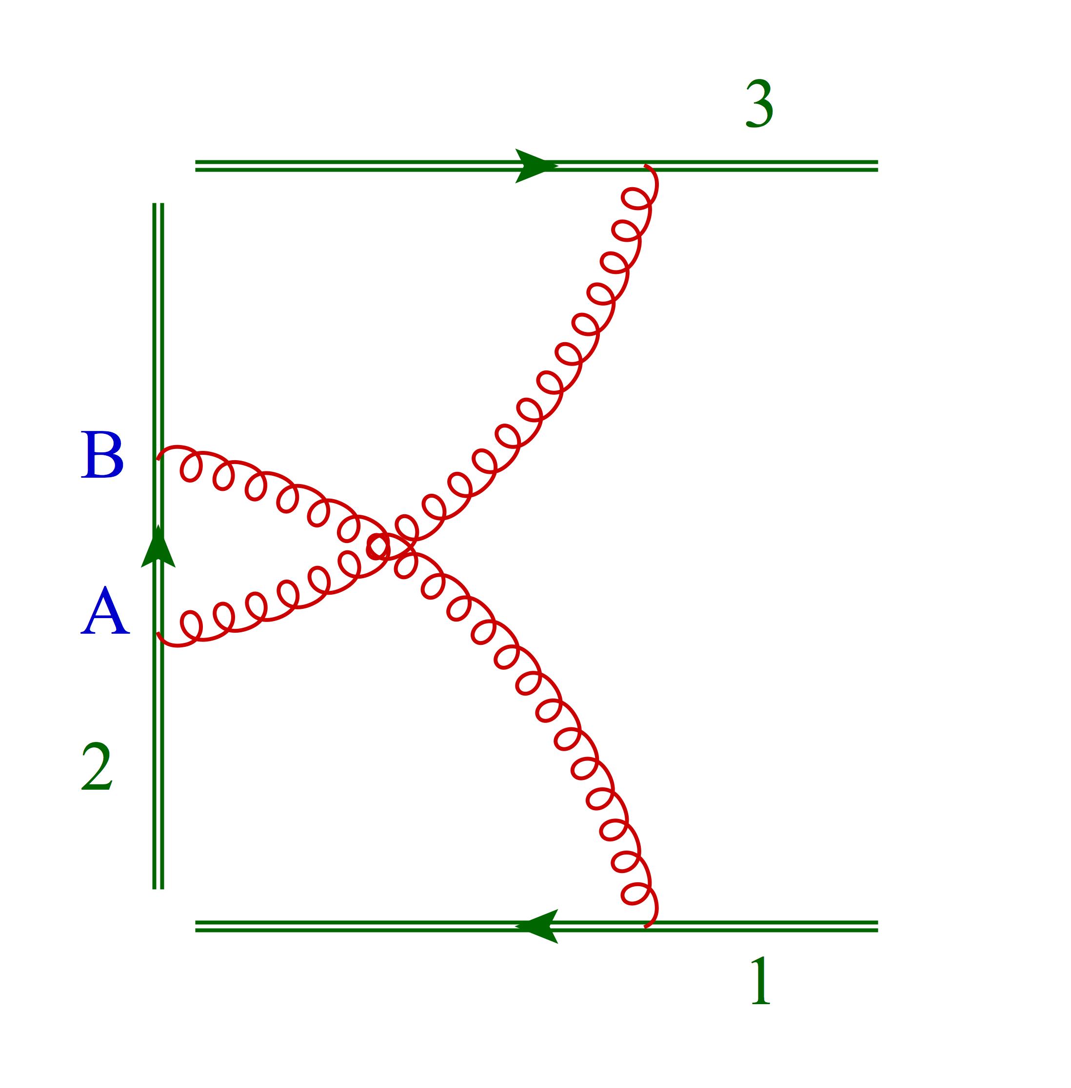
(a)

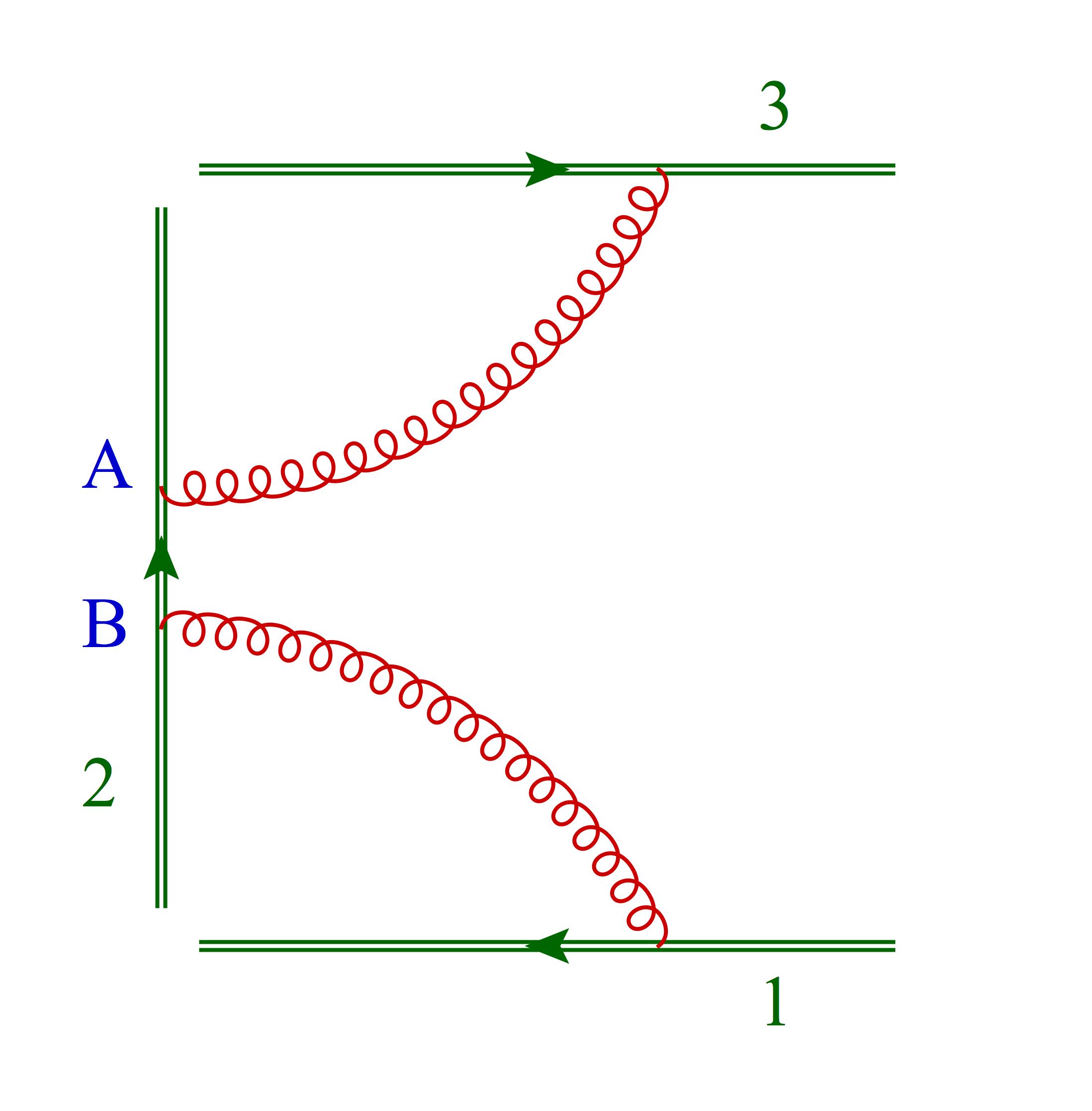
(b)

Figure 30: A simple two-loop, three-line web involving two Feynman diagrams. Note that Wilson lines are oriented, and labelled by integers in green; multiple gluon attachments to a given line (whose permutations generate the web) are labelled by capital letters in blue.

Web mixing matrices are clearly crucial quantities for the purpose of computing Wilson-line correlators, and therefore, in particular, the soft anomalous dimension matrix. Their properties were extensively studied in Refs. [199, 486, 482, 487, 488, 489, 490, 493], while an interesting alternative approach to exponentiation was developed in Refs. [494, 495]. We conclude this subsection by listing the properties of the mixing matrices that appear in Eq. (5.85), while in Section 5.3.3 we will describe an algorithm to compute them explicitly, after introducing a more suitable diagrammatic organisation of the perturbative exponent in Section 5.3.2. Properties 1 to 3 below were proved in Refs. [199, 487, 490], while Property 4 was conjectured in [199], and verified to hold up to four loops in Refs. [496, 497].

1. Idempotency. Web mixing matrices are idempotent, i.e.

   $$R_{w}^{2}\,=\,R_{w}\,.$$ (5.88)

   This property implies that the eigenvalues can only be either 1 or 0: in other words, web mixing matrices are projection operators, selecting a subset of the available colour factors. If we denote by $Y_{w}$ the matrix diagonalising $R_{w}$, we have then

   $$Y_{w}R_{w}Y_{w}^{-1}\,=\,{\rm diag}\left(\lambda_{1},...,\lambda_{p_{w}}\right)\,=\,{\bf 1}_{r_{w}}\oplus{\bf 0}_{p_{w}-r_{w}}\,,$$ (5.89)

   where $p_{w}$ is the number of diagrams for web $w$, and thus the dimension of the matrix $R_{w}$, while $r_{w}<p_{w}$ is the rank of $R_{w}$. We can now write Eq. (5.86) as

   $$w = \big{(}{\cal K}_{w}^{T}\,Y_{w}^{-1}\big{)}\,Y_{w}R_{w}Y_{w}^{-1}\,\big{(}Y_{w}\,C_{w}\big{)}$$ (5.90)

   $$= \sum_{h=1}^{r_{w}}\big{(}{\cal K}_{w}^{T}Y_{w}^{-1}\big{)}_{h}\big{(}Y_{w}C_{w}\big{)}_{h}\,,$$

   where ${\cal K}_{w}$ is the vector of kinematic factors and $C_{w}$ the vector of colour factors for web $w$. It is clear that only $r_{w}$ ECFs will contribute to web $w$.

2. Non-abelian exponentiation. The non-abelian exponentiation theorem [490] identifies the colour factors which survive the projection discussed above: to all orders in perturbation theory, they are the colour factors which, by the Feynman rules, would be associated to connected gluon subdiagrams.

3. Row sum rule. The elements of web mixing matrices obey the row sum rule

   $$\sum_{D^{\prime}}R_{w}(D,D^{\prime})\,=\,0\,,$$ (5.91)

   for any web $w$ with $p_{w}>1$, implying that at least one of the eigenvalues of any non-trivial web mixing matrix must vanish.

4. Column sum rule. One may also envisage the web mixing matrix as acting on the vector of kinematic factors for the diagrams of web $w$. Taking this viewpoint, the projection effected by the matrix $R_{w}$ has another non-trivial effect: it selects combinations of kinematic factors that do not contain ultraviolet sub-divergences. This is crucial for the consistency of the method we are outlining: thanks to this property, at each successive order in perturbation theory webs contribute a single extra UV pole, so that the corresponding counterterm can be extracted, in a minimal scheme, with no dependence on the infrared regulator. The absence of sub-divergences was established for the two-line case in Refs. [483, 484, 485]; for $n>2$ Wilson lines a complete all-order proof is still lacking, but the property holds for all webs up to four loops [199, 496, 497]. A necessary ingredient for the proof is that the elements of web mixing matrices obey a column sum rule, which can be characterised as follows.

   Given a diagram $D$, consider the set of its connected sub-diagrams (after removing the Wilson lines), $\{D_{\rm c}^{i}\subset D\}$; we say that a connected sub-diagram $D_{\rm c}^{i}$ can be shrunk to the common origin of the Wilson lines if all the vertices connecting the sub-diagram to the Wilson lines can be moved to the origin without encountering vertices associated with other sub-diagrams.

   For any given diagram $D$, we then define the column weight of diagram $D$, $s(D)$, as the number of different ways in which the connected sub-diagrams $D_{\rm c}^{i}$ of $D$ can be sequentially shrunk, so that all gluon attachments to Wilson lines in $D$ are moved to their common origin. Thus, if all gluon attachments are entangled, so that no subdiagram can be shrunk without shrinking the whole diagram, then $s(D)=0$. On the other hand, if, for example, a single subdiagram $D_{\rm c}^{i}$ can be shrunk without affecting the others, this provides a non-trivial sequence for the the shrinking of the whole diagram, so that $s(D)=1$: this is the situation for the two diagrams portrayed in Fig. 30.

   Armed with these definitions, we can state the (conjectured) column sum rule for web mixing matrices as

   $$\sum_{D\in w}\,s(D)\,R_{w}(D,D^{\prime})\,=\,0\,.$$ (5.92)

   The connection of this rule to UV sub-divergences is clear in a coordinate-space picture [224]: in this picture, one understands UV divergences as arising from short distances between interaction vertices, and ‘shrinkable’ sub-diagrams are naturally associated to UV sub-divergences. Eq. (5.92) guarantees that these sub-diagrams are projected out of the webs.

5.3.2 From gluon webs to correlator webs

Even from the preliminary description given in Section 5.3.1, it should be apparent that the diagrammatic structure of the perturbative exponent has two independent components: on the one hand, connected gluon subdiagrams with external (off-shell) gluons, and on the other hand the arrangement of possible attachments of these gluons to the Wilson lines. Motivated by this observation, Ref. [496] proposed to organise the perturbative exponent not in terms of sets of diagrams, but in terms of sets of connected gluon correlators, which were called Cwebs. Conceptually, Cwebs are the proper building blocks for the logarithm of the Wilson-line correlator: indeed, their introduction simplifies considerably the counting and organisation of diagrammatic contributions, especially at high orders, where radiative corrections to gluon sub-diagrams become important and proliferate; furthermore, using Cwebs does not affect the definition and structure of web mixing matrices, which are derived exclusively from the ordering of gluon attachments to the Wilson lines, and are not affected by gluon interactions away from the Wilson lines. In this Section, we will briefly review the properties of Cwebs, while in Section 5.3.3 we will describe an algorithm to compute Cweb mixing matrices, which is a simple adaptation of the algorithm given in Ref. [486], implicitly showing that Cwebs are a natural and proper generalisation of webs.

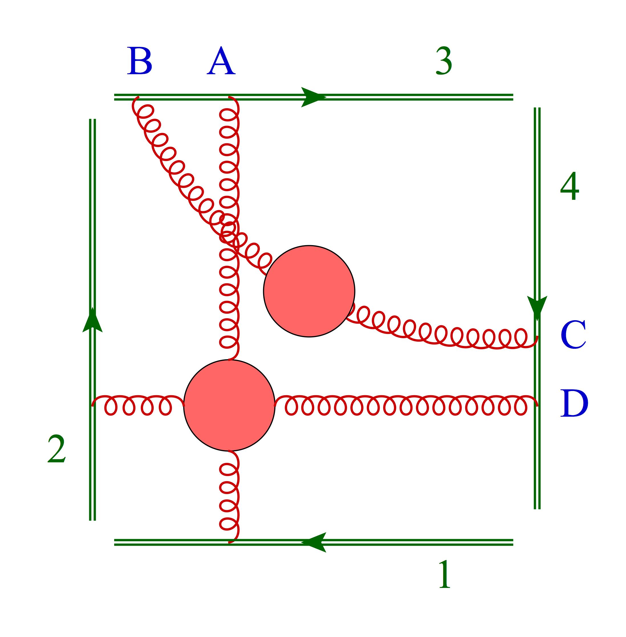
Figure 31: A four-line Cweb containing one four-gluon correlator and one two-gluon correlator.

We begin with the definition

• Correlator Web (Cweb): A set of skeleton diagrams, built out of connected gluon correlators attached to Wilson lines, and closed under permutations of the gluon attachments to each Wilson line.

As an example, a four-line Cweb built with two connected gluon correlators is shown in Fig. 31. Clearly, Cwebs are not fixed-order quantities, but admit their own perturbative expansion in powers of the gauge coupling $g$. Below, we will use the notation $W_{n}^{(c_{2},\ldots,c_{p})}(k_{1},\ldots,k_{n})$ for a Cweb constructed out of $c_{m}$ $m$-point connected gluon correlators ($m=2,\ldots,p$), where $k_{i}$ is the number of gluon attachments to the $i$-th Wilson line. Note that there is an obvious degeneracy in the counting of Cwebs, since Cwebs that differ only by a permutation of their Wilson lines are structurally identical, and it is trivial to include them in the calculation of the full correlator, simply by summing over Wilson-line labels. For the sake of classification, we can then focus on a specific Wilson-line ordering, choosing for example $k_{1}\leq k_{2}\leq\ldots\leq k_{n}$. As an example, in this notation the Cweb in Fig. 31 is denoted by $W_{4}^{(1,0,1)}(1,1,2,2)$. Taking into account the fact that the perturbative expansion for an $m$-point connected gluon correlator starts at ${\cal O}(g^{m-2})$, while each attachment to a Wilson line carries a further power of $g$, the perturbative expansion for a Cweb can be written as

$$W_{n}^{(c_{2},\ldots,c_{p})}(k_{1},\ldots,k_{n})\,=\,g^{\,\sum_{i=1}^{n}k_{i}\,+\,\sum_{r=2}^{p}c_{r}(r-2)}\,\sum_{j=0}^{\infty}\,W_{n,\,j}^{(c_{2},\ldots,c_{p})}(k_{1},\ldots,k_{n})\,g^{2j}\,,$$ (5.93)

which defines the perturbative coefficients $W_{n,\,j}^{(c_{2},\ldots,c_{p})}(k_{1},\ldots,k_{n})$. With this in mind, it is natural to classify Cwebs based on the perturbative order where they receive their lowest-order contribution, which is given by the power of $g$ in the prefactor of Eq. (5.93); one may then easily design a recursive procedure for construction of Cwebs.

Starting at lowest order, we notice that only two Cwebs appear at order $g^{2}$: the self-energy insertion with a two-point connected gluon correlator attached to a single Wilson line, which we denote by $W_{1}^{(1)}(2)$, and the configuration where the two-gluon correlator joins two Wilson lines, denoted by $W_{2}^{(1)}(1,1)$. These two Cwebs are depicted in Fig. 32.

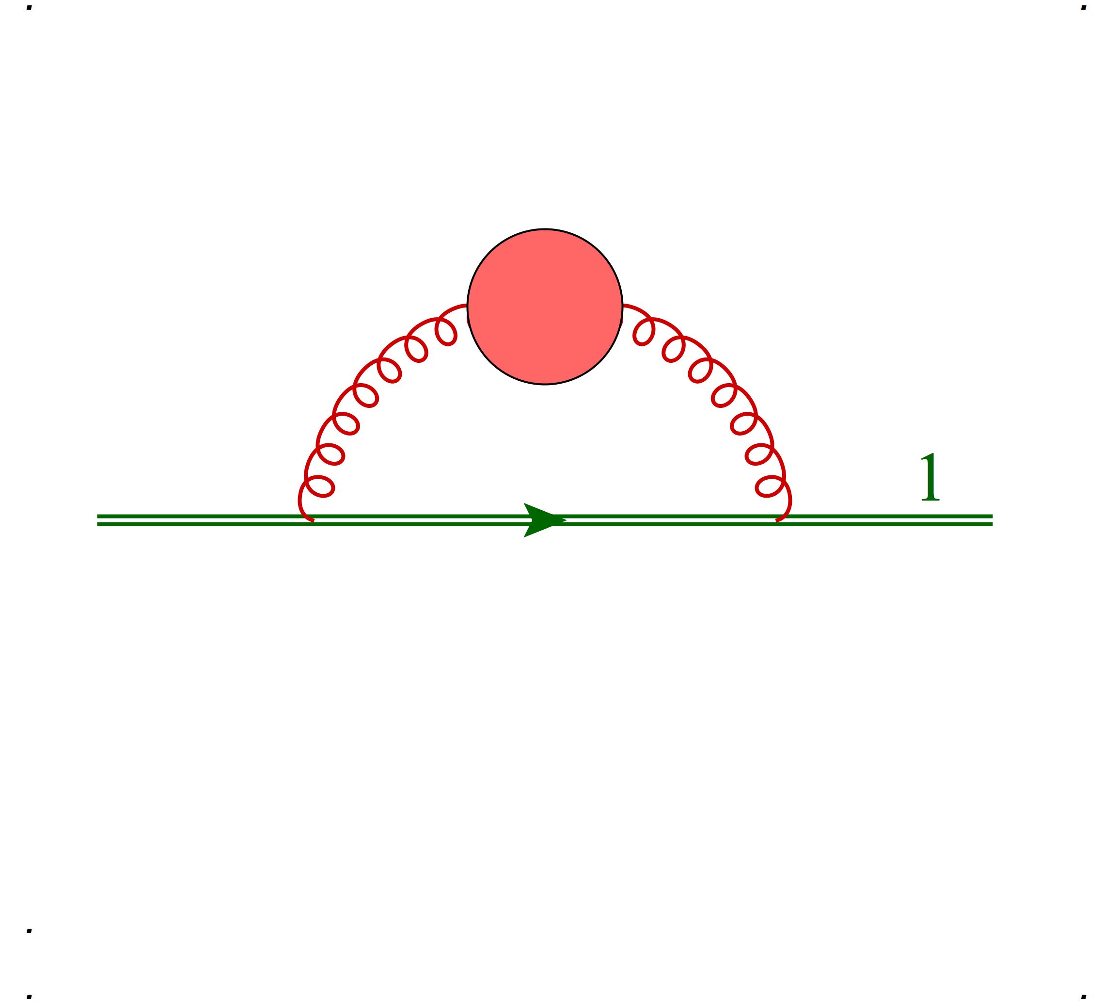
(a)

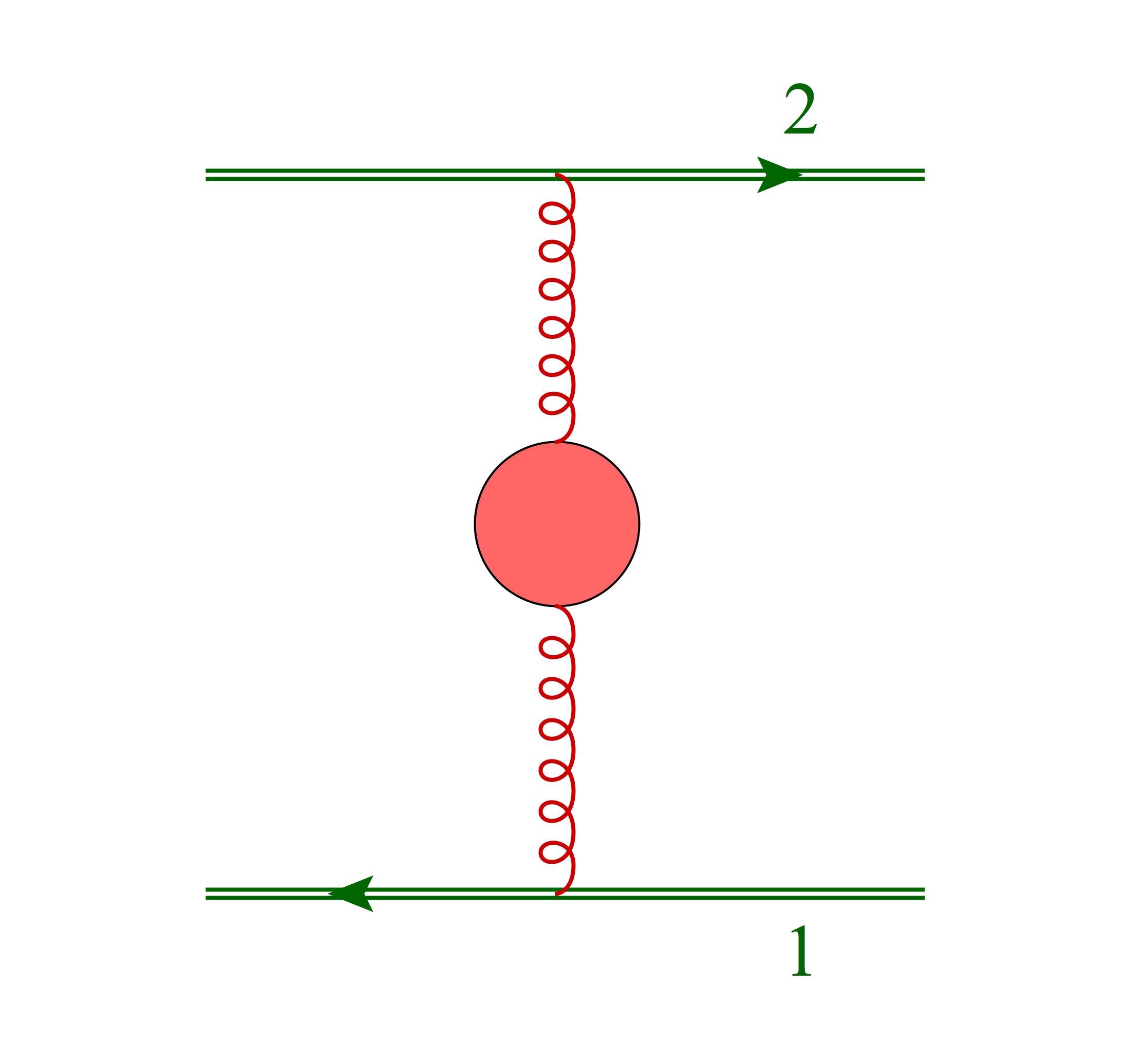
(b)

Figure 32: The only two Cwebs whose perturbative expansion starts at ${\cal O}(g^{2})$.

Notice that, if the Wilson lines are light-like, the self-energy Cweb vanishes identically, since, by the eikonal Feynman rules, it is proportional to the square of the Wilson-line four-velocity vector, $\beta^{2}$: in that case, one is left with just one non-vanishing ${\cal O}(g^{2})$ Cweb. Starting from this initial condition, one may recursively construct all Cwebs starting at higher perturbative orders: indeed, having constructed all Cwebs at ${\cal O}(g^{2n})$, there are three ways of adding a power of $g^{2}$.

• Add a two-gluon connected correlator connecting any two Wilson lines (including ‘new’ Wilson lines that had no attachments in lower-order Cwebs).

• Connect an existing $m$-point correlator to any Wilson line (again, including Wilson lines with no attachments at lower orders), turning it into an $(m+1)$-point correlator.

• Connect an existing $m$-point correlator to an existing $n$-point correlator, resulting in an $(n+m)$-point correlator.

Executing all possible moves is clearly redundant, since the same Cweb is generated more than once through different sequences of moves: upon performing all moves, one must therefore remove Cwebs that have been counted more than once. The procedure can be considerably streamlined by taking into account known properties of webs, which naturally generalise to Cwebs. For example, webs (and thus Cwebs) that are given by the product of two or more disconnected lower-order webs (so that there are subsets of Wilson lines not joined by any gluons) do not contribute to the logarithm of the correlator, ${\cal W}_{n}$; furthermore, as mentioned above, in a massless theory all self-energy Cwebs, where all gluon lines attach to the same Wilson line, vanish as a consequence of the eikonal Feynman rules. Thus, any Cweb containing a connected gluon correlator attaching to a single Wilson line will vanish. Using these recursive rules, it is easy to enumerate inequivalent Cwebs at low orders. In the massless theory, for example, one finds four inequivalent Cwebs at ${\cal O}(g^{4})$, fourteen new Cwebs at ${\cal O}(g^{6})$, and a total of sixty new Cwebs at ${\cal O}(g^{8})$: they are discussed in detail in Ref. [496].

At each order in $g$, Cwebs contain webs, all sharing the same mixing matrix, since the colour algebra associated with permutations of attachments to the Wilson lines is unaffected by radiative corrections to the connected correlators comprising the Cweb. We can thus construct Cweb mixing matrices by the same technique devised in [486] for webs, which we now discuss.

5.3.3 A replica algorithm to generate web mixing matrices

As is the case for other combinatorial problems involving exponentiation, such as the construction of effective actions, Wilson-line correlators can be studied by means of algorithms constructed with the replica method [499]. In this section, we will summarise the application of the replica method to the construction of Cweb mixing matrices, following Refs. [109, 486].

In order to introduce the method, consider the path integral expression for the Wilson-line correlator in Eq. (5.81)

$${\cal S}_{n}\left(\gamma_{i}\right)\,=\,\exp\Big{[}W_{n}(\gamma_{i})\Big{]}\,=\,\int{\cal D}A_{\mu}^{a}\,\,{\rm e}^{{\rm i}S\left(A_{\mu}^{a}\right)}\,\prod_{k=1}^{n}\Phi\left(\gamma_{k}\right)\,,$$ (5.94)

where $S$ is the classical action. In order to compute $W_{n}(\gamma_{i})$, one starts by building a replicated theory, replacing the single gluon field $A_{\mu}^{a}$ with $N_{r}$ identical copies $A_{\mu}^{a,\,i}$ ($i=1,\ldots,N_{r}$), which do not interact with each other. Under this replacement, one has $S\left(A_{\mu}^{a}\right)\rightarrow\sum_{i=1}^{N_{r}}S\left(A_{\mu}^{a,\,i}\right)$; if, furthermore, we replace each Wilson line in Eq. (5.94) by the product of $N_{r}$ Wilson lines, each belonging to one replica of the theory, one readily sees that the replicated correlator is given by

$${\cal S}_{n}^{\,{\rm repl.}}\left(\gamma_{i}\right)\,=\,\Big{[}{\cal S}_{n}\left(\gamma_{i}\right)\Big{]}^{N_{r}}\,=\,\exp\Big{[}N_{r}\,W_{n}(\gamma_{i})\Big{]}\,=\,{\bf 1}+N_{r}\,W_{n}(\gamma_{i})+{\cal O}(N_{r}^{2})\,.$$ (5.95)

Eq. (5.95) provides a straightforward method to compute $W_{n}(\gamma_{i})$: one may compute the replicated correlator (essentially a combinatorial problem, as we will see), and then extract from the result the term of order $N_{r}$.

An important point is that, while gluon fields in different replicas do not interact, they all belong to the same gauge group: therefore, the colour matrices associated with their attachments to a Wilson line do not commute, and their ordering is relevant. On the other hand, in a Cweb, each connected gluon correlator can be assigned a unique replica number, since there are no interaction vertices connecting different replicas. One can then relate the contributions of different skeleton diagrams to the replicated correlator in Eq. (5.95) to those of the same diagrams in the un-replicated theory, by means of combinatorial factors, counting the multiplicities associated with the presence of different replicas. The computation of $W_{n}(\gamma_{i})$ in terms of the skeleton diagrams contributing to ${\cal S}_{n}(\gamma_{i})$ is thus reduced to the computation of these combinatorial factors. The necessary steps, listed below, were identified for webs in Refs. [109, 486], and naturally adapt to the language of Cwebs.

• For any given Cweb, assign a replica number $i$ ($1\leq i\leq N_{r}$) to each connected gluon correlator present in the Cweb.

• Define a replica ordering operator $R$, acting on color generators on each Wilson line as

  $$R\Big{(}{\bf T}_{k}^{(i)}{\bf T}_{k}^{(j)}\Big{)}\! = \!{\bf T}_{k}^{(j)}{\bf T}_{k}^{(i)}\quad\textrm{if}\,\,i>j\,,$$ (5.96)

  $$R\Big{(}{\bf T}_{k}^{(i)}{\bf T}_{k}^{(j)}\Big{)}\! = \!{\bf T}_{k}^{(i)}{\bf T}_{k}^{(j)}\quad\textrm{if}\,\,i\leq j\,,$$

  where ${\bf T}_{k}^{(i)}$ is the group generator associated with the emission of a gluon in replica $i$ from the $k$-th Wilson line. The operator $R$ effectively replaces the selected skeleton diagram with another one drawn from the same Cweb: as a consequence, one may verify that the colour factor in the replicated theory is a linear combination of the colour factors of all skeleton diagrams in the Cweb, with multiplicities given by the number of possible replica orderings of the gluon attachments on every Wilson line.

• In order to proceed, one needs to list all possible hierarchies of the replica numbers associated with each correlator in the Cweb: these hierarchies in fact define the action of the $R$ operator on each skeleton diagram of the Cweb. For a Cweb built out of $m$ connected correlators, the number $h(m)$ of possible hierarchies between the $m$ replica numbers of the correlators grows rapidly with $m$, and is not entirely trivial to determine, since the case of equal replica numbers must be treated separately. The result is however well known [500]: $h(m)$ are the so-called Fubini numbers. In the first instances, for $m=\{1,2,3,4,5,6\}$ one finds $h(m)=\{1,3,13,75,541,4683\}$. For every fixed hierarchy $h$, the number relevant for the determination of the colour factor in the replicated theory is the multiplicity with which that hierarchy can occur in the presence of $N_{r}$ replicas, which we denote by $M_{N_{r}}(h)$. It is not difficult to see that it is given by

  $$M_{N_{r}}(h)\,=\,\frac{N_{r}!}{\big{(}N_{r}-n_{r}(h)\big{)}!\,\,n_{r}(h)!}\,,$$ (5.98)

  where $n_{r}(h)$ is the number of distinct replicas present for hierarchy $h$. To give a concrete example, for $m=5$, labelling the replica numbers of the five correlators with $r_{k}$, $(k=1,\ldots,5)$, and picking the hierarchy $r_{1}=r_{2}<r_{3}=r_{4}<r_{5}$, we have $n_{r}(h)=3$, and thus $M_{N_{r}}(h)=N_{r}(N_{r}-1)(N_{r}-2)/6$.

• Finally, the exponentiated color factors for a skeleton diagram $D$ is given by

  $$C_{N_{r}}^{\,{\rm repl.}}(D)\,=\,\sum_{h}M_{N_{r}}(h)\,R\big{[}C(D)\big{|}h\big{]}\,,$$ (5.99)

  where $R\big{[}C(D)\big{|}h\big{]}$ is the color factor of the skeleton diagram obtained from $D$ through the action of the replica-ordering operator $R$, in the case of hierarchy $h$. The Cweb mixing matrix is built by picking terms that are linear in $N_{r}$ out of the coefficients $M_{N_{r}}(h)$, which are polynomials in $N_{r}$. Note that in the presence of $m$-point correlators, with $m\geq 4$, each correlator can contribute different ‘internal’ colour factors, for example different permutations of products of structure constants. Since, however, the information on the mixing matrix is encoded in the coefficients $M_{N_{r}}(h)$, the different colour factors arising from the internal structure of the correlators can be treated one by one, without affecting the mixing of the diagrams.

To conclude our discussion of exponentiated colour factors, we briefly comment on the dimensionality of Cweb mixing matrices. One would naïvely imagine that it should be given by the product of the numbers of possible gluon permutations on each Wilson line. This however neglects two important subtleties. First, if a set of, say, $k$ gluons emerging from a given correlator attaches on a single Wilson line, their permutations are irrelevant, since the correlator is Bose symmetric. One should not then count permutations on each line, but rather shuffles of the subsets of gluons emerging from each correlator and attaching to a given line. Furthermore, there is another important degeneracy, which already appears in the simple two-line Cweb $W^{(2)}_{2}(2,2)$ at two loops: counting shuffles separately on each line would yield, in that case, the result $d=4$ for the dimensionality of the mixing matrix, which is wrong, because the two shuffles on the second Wilson line can be obtained from the shuffles on the first line by exchanging the two gluons, which is manifestly a symmetry of the Cweb. In order to take into account this degeneracy, one must divide by the number of available permutations of subsets of $m$-point correlators that have the property of being attached to the same sets of Wilson lines.

The discussion in the last three sections has been general and rather formal, but also incomplete, since of course much of the dynamical content of the soft anomalous dimension matrix resides in the kinematic factors, which emerge from loop integrals of rapidly increasing complexity at high orders. To fill these gaps, we now give two simple examples of the evaluation of these kinematic factors at one and two loops. At the two-loop level, this will also serve to illustrate in a concrete case the interplay of colour and kinematics which has been discussed formally in the previous sections.

5.3.4 The one-loop angle-dependent cusp anomalous dimension

We begin by describing the calculation of the only non-vanishing one-loop diagram contributing to the soft anomalous dimension matrix in the massless case. The relevant diagram corresponds to the tree-level contribution to the Cweb in Fig. 32(b), and of course it is a web on its own. Clearly, this diagram is very simple, and it can be computed in a number of ways - indeed, we performed an equivalent calculation in Section 3.3.2 with light-like Wilson lines. We display the complete calculation here, with collinear divergences regulated by using ‘massive’ Wilson lines, and soft divergences regulated by the exponential suppression defined in Eq. (5.70), in order to illustrate techniques that can be profitably used at higher orders as well. Besides, the calculation yields the one-loop result for the angle-dependent cusp anomalous dimension, which is a fundamental quantity for the scattering of massive particles and in many other contexts [370]. Unlike Section 3.3.2, we will proceed by recognising in the second line of Eq. (3.3.2) the coordinate-space gluon propagator, $D_{\mu\nu}(x)$, evaluated for $x=\lambda_{i}\beta_{i}-\lambda_{j}\beta_{j}$. The expression for this propagator in $d=4-2\epsilon$ is well known, and is given by

$$D_{\mu\nu}^{ab}(x)\,=\,-\,\frac{\Gamma(1-\epsilon)}{4\,\pi^{2-\epsilon}}\,g_{\mu\nu}\,\delta^{ab}\,\frac{1}{(-x^{2}+i\eta)^{1-\epsilon}}\,.$$ (5.100)

Using this expression leaves only two parameter integrals to be performed. Arguably, this ‘coordinate space’ approach to eikonal integrals simplifies their calculations also at higher orders, and it was indeed adopted for the state-of-the-art calculation of Ref. [77].

In Cweb notation, the diagram in Fig. 32 (b), including radiative corrections to the gluon propagator, can be written as

$$W_{2,\,ij}^{(1)}(1,1)\,=\,{\bf T}_{i}\cdot{\bf T}_{j}\;{\cal K}^{(1)}_{2}\bigg{(}\gamma_{ij},\frac{\mu^{2}}{m^{2}},\epsilon\bigg{)}\,,$$ (5.101)

where ${\cal K}^{(1)}_{2}(\gamma_{ij},\mu^{2}/m^{2},\epsilon)$ gives the regularised kinematic factor. The color structure is straightforward and there is no mixing matrix involved, since this is a single-diagram web. With the infrared regulator in place, and having introduced the gluon propagator in Eq. (5.100), the one-loop kinematic factor reads

$${\cal K}^{(1)}_{2,1}\bigg{(}\gamma_{ij},\frac{\mu^{2}}{m^{2}},\epsilon\bigg{)}=g_{s}^{2}\mu^{2\epsilon}\,\frac{\Gamma(1-\epsilon)}{4\,\pi^{2-\epsilon}}\,\beta_{i}\cdot\beta_{j}\int_{0}^{\infty}\!d\lambda_{i}\int_{0}^{\infty}\!d\lambda_{j}\,\frac{{\rm e}^{-m\lambda_{i}\sqrt{\beta_{i}^{2}}-m\lambda_{j}\sqrt{\beta_{j}^{2}}}}{\Big{(}\!-\left(\lambda_{i}\beta_{i}-\lambda_{j}\beta_{j}\right)^{2}+i\eta\Big{)}^{1-\epsilon}}\,.$$ (5.102)

To perform the integral, it is clearly useful to rescale the variables and define

$$\sigma\,=\,\lambda_{i}\sqrt{\beta_{i}^{2}}\,,\qquad\tau\,=\,\lambda_{j}\sqrt{\beta_{j}^{2}}\,.$$ (5.103)

We then introduce coordinates $\lambda$ and $x$, which are respectively normal and intrinsic to the pinch surface (in this case a point),

$$\lambda\,=\,\sigma+\tau\,,\qquad\quad x\,=\,\frac{\sigma}{\sigma+\tau}\,;$$ (5.104)

the normal coordinate $\lambda$ gives the “overall distance” of the gluon from the cusp, and ranges from 0 to $\infty$. The intrinsic angular coordinate ranges between 0 and 1, and measures the degree of collinearity of the gluon to either Wilson line. The integral over $\lambda$ can be readily performed and gives a factor of $\Gamma(2\epsilon)$ containing the ultraviolet pole. The integration over the intrinsic variable $x$ remains, and we can write

$${\cal K}^{(1)}_{2,1}\bigg{(}\gamma_{ij},\frac{\mu^{2}}{m^{2}},\epsilon\bigg{)}\,=\,-\bigg{(}\frac{\mu^{2}}{m^{2}}\bigg{)}^{\epsilon}g_{s}^{2}\,\,\frac{\Gamma(1-\epsilon)}{8\pi^{2-\epsilon}}\,\Gamma(2\epsilon)\,\gamma_{ij}\int_{0}^{1}dx\,P\big{(}x,\gamma_{ij}\big{)}\,,$$ (5.105)

where

$$P\big{(}x,\gamma_{ij}\big{)}\,=\,\Big{[}x^{2}+(1-x)^{2}-x(1-x)\gamma_{ij}-{\rm i}\eta\Big{]}^{-1+\epsilon}\,.$$ (5.106)

The quadratic polynomial in $x$ in Eq. (5.106) can be factored with the change of variables

$$\gamma_{ij}\,\equiv\,-\,\alpha_{ij}-\frac{1}{\alpha_{ij}}\,,$$ (5.107)

where we can take $\alpha_{ij}$ to lie inside the unit circle in the complex plane, thanks to the symmetry under $\alpha_{ij}\to 1/\alpha_{ij}$. The $x$ integral can then be performed exactly, and gives a hypergeometric function,

$${\cal K}^{(1)}_{2,1}\bigg{(}\gamma_{ij},\frac{\mu^{2}}{m^{2}},\epsilon\bigg{)}\,=\,-\left(\frac{\mu^{2}}{m^{2}}\right)^{\epsilon}\,g_{s}^{2}\,\frac{\Gamma(1-\epsilon)}{8\pi^{2-\epsilon}}\,\,\Gamma(2\epsilon)\,\gamma_{ij}\,{}_{2}F_{1}\bigg{(}1,1-\epsilon,\frac{3}{2},\frac{1}{2}+\frac{\gamma_{ij}}{4}\bigg{)}\,.$$ (5.108)

Expanding Eq. (5.108) around $\epsilon=0$ we can easily obtain the coefficient of the simple pole in Eq. (5.105). Reinstating then the colour factor, making use of Eq. (5.80) at one loop, and summing over available colour dipoles, we obtain the soft anomalous dimension matrix at one loop, for massive Wilson lines. In terms of the $\alpha_{ij}$ variables, it is given by

$$\Gamma^{(1)}_{\cal S}\,=\,\sum_{i<j}\,{\bf T}_{i}\cdot{\bf T}_{j}\,\frac{1+\alpha_{ij}^{2}}{1-\alpha_{ij}^{2}}\,\ln\alpha_{ij}\,.$$ (5.109)

In this representation, the limit of light-like Wilson lines is reached as $\alpha_{ij}\to 0$, corresponding to $\gamma_{ij}\to\infty$. The logarithmic singularity in that limit corresponds to the collinear divergence in Eq. (3.3.2), and the coefficient of the logarithm in the $\alpha_{ij}\to 0$ limit gives the light-like cusp anomalous dimensions discussed in earlier Sections. An alternative representation is often given, in terms of the Minkowski-space cusp angles between Wilson lines $i$ and $j$, which we denote by $\xi_{ij}$, defined by

$$\xi_{ij}\,=\,\cosh^{-1}\!\bigg{(}\!-\frac{\gamma_{ij}}{2}\bigg{)}\,.$$ (5.110)

Using this variable one finds

$$\Gamma^{(1)}_{\cal S}\,=\,-\,\sum_{i<j}{\bf T}_{i}\cdot{\bf T}_{j}\,\,\xi_{ij}\coth\big{(}\xi_{ij}\big{)}\,.$$ (5.111)

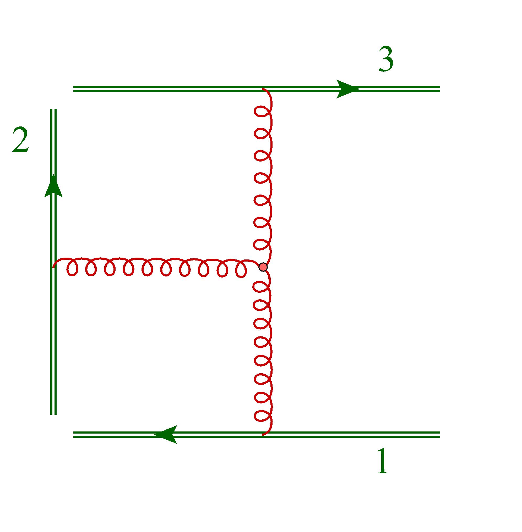
Figure 33: A two-loop, three-line web involving a 3-gluon vertex.

As we will see below, the one-loop angle-dependent cusp anomalous dimension, given here in Eq. (5.109) and in Eq. (5.111) plays an important role also for higher-order corrections to the soft anomalous dimension matrix for massive particles.

5.3.5 The two-loop soft anomalous dimension matrix

$i$, $j$	Replica-ordered colour factor	Multiplicity
$i=j$	$C(a)$	$N_{r}$
$i<j$	$C(b)$	$N_{r}(N_{r}-1)/2$
$i>j$	$C(a)$	$N_{r}(N_{r}-1)/2$

Table 1: Replica analysis of diagram $(a)$ of Fig. 30, as described in the text.

We now proceed to summarise the calculation of the two-loop soft anomalous dimension matrix, which will give us an opportunity to illustrate the application of the replica method discussed in Section 5.3.3 with the simplest non-trivial example.

At two-loops, a maximum of three Wilson lines can be connected, and we get a total of two distinct webs: one was shown in Fig. 30, while the other one, involving a single diagram with a three-gluon vertex, is shown in Fig. 33. Here we will discuss in some detail the web in Fig. 30, which is the lowest-order contribution to the Cweb $W_{3}^{(2)}(1,2,1)$, and is also an example of the class of webs called “multiple gluon exchange webs” (MGEW), discussed in Ref. [480]. The contribution of this two-loop web can be written schematically as

$$w_{121}^{(2)}\,=\,{\cal K}(a)\,\widetilde{C}(a)+{\cal K}(b)\,\widetilde{C}(b)\,,$$ (5.112)

where ${\cal K}(a)$ and ${\cal K}(b)$ are the kinematic contributions of the two diagrams of the web and $\widetilde{C}(a)$ and $\widetilde{C}(b)$ are the corresponding exponentiated color factors. Considering as an example diagram $(a)$ in Fig. 30, and introducing $N_{r}$ replicas, we note that the replica-ordering operator will replace the colour factor of $(a)$ with that of $(b)$ in Fig. 30, in the $N_{r}(N_{r}-1)/2$ cases in which the replicas assigned to the two gluons are in the ‘wrong’ order, as reported in Table 1. The colour factor of diagram $(a)$ in the replicated theory then reads

$$C^{\,\rm repl.}_{N_{r}}(a)\,=\,N_{r}C(a)+\frac{N_{r}(N_{r}-1)}{2}\big{(}C(a)+C(b)\big{)}\,=\,N_{r}\left(\frac{C(a)-C(b)}{2}\right)+{\cal O}(N_{r}^{2})\,,$$ (5.113)

and similarly for diagram $(b)$. The coefficients of ${\cal O}(N_{r})$ terms give us then the exponentiated color factors

$$\widetilde{C}(a)\,=\,\left(\frac{C(a)-C(b)}{2}\right)\,=\,-\,\widetilde{C}(b)\,.$$ (5.114)

Thus

$$w_{121}^{(2)}\,=\,\frac{1}{2}\,\big{(}C(a)-C(b)\big{)}\big{(}{\cal K}(a)-{\cal K}(b)\big{)}\,.$$ (5.115)

corresponding to the web mixing matrix

$$\begin{split}&R_{121}\,=\,\frac{1}{2}\,\displaystyle{\left(\!\!\begin{array}[]{cc}1&-1\\ -1&1\\ \end{array}\!\!\right)}\,.\end{split}$$ (5.116)

We note in passing that, as expected, $R_{121}$ satisfies the row sum rule in Eq. (5.91). In order to check the column sum rule in Eq. (5.92), we must construct the vector $s(D)$ for the two diagrams in Fig. 30. Taking into account the orientation of the Wilson lines, one sees that for both diagrams there is only one way in which the two gluons can be sequentially shrunk to the origin, so that we get

$$s(a)\,=\,s(b)\,=\,1\,,$$ (5.117)

and, also as expected, the column sum rule is verified. Concerning the exponentiated colour factors, one easily sees that the non-abelian exponentiation theorem is verified for this simple web. Indeed, the color factors of the diagrams (a) and (b) are

$$C(a)\,=\,T_{1}^{a}T_{2}^{a}T_{2}^{b}T_{3}^{b}\,,\qquad C(b)\,=\,T_{1}^{a}T_{2}^{b}T_{2}^{a}T_{3}^{b}\,.$$ (5.118)

Recalling that color generators pertaining to the same Wilson line do not commute, and using the colour algebra, we can write the exponentiated color factor as

$$\widetilde{C}(a)\,=\,-\frac{1}{2}\,{\rm i}f_{abc}T_{1}^{a}T_{2}^{b}T_{3}^{c}\,=\,-\,\widetilde{C}(b)\,,$$ (5.119)

a result which is proportional to the colour factor of the fully connected diagram in Fig. 33.

We now turn to the computation of the kinematic factor of this web, following Ref. [242]. This will allow us to illustrate the dynamical effects of the column sum rule on leading infrared poles. We follow the same strategy as in Section 5.3.4, associating directly to each gluon its coordinate-space propagator, and thus leaving only parameter integrals to be performed. We parametrise the positions of gluon attachments on Wilson lines $1,2$ and $3$ by $s\beta_{1}$, $t_{1}\beta_{2}$, $t_{2}\beta_{2}$ and $u\beta_{3}$, respectively, and introduce exponential suppressions for each Wilson line. In diagram (a), the gluon that attaches at $t_{1}$ is further away from the origin than the one at $t_{2}$, which is accounted for by including step function $\theta(t_{1}-t_{2})$. We get then, for diagram (a),

$${\cal K}(a)\! = \!g_{s}^{4}\mu^{4\epsilon}\,\frac{\Gamma^{2}(1-\epsilon)}{16\,\pi^{4-2\epsilon}}\,\beta_{1}\cdot\beta_{2}\,\beta_{2}\cdot\beta_{3}\,\int_{0}^{\infty}ds\,dt_{1}\,dt_{2}\,du\,\,\theta(t_{1}-t_{2})$$ (5.120)

$$\times\,\frac{\exp\Big{[}{-m\Big{(}s\sqrt{\beta_{1}^{2}}+u\sqrt{\beta_{3}^{2}}+\big{(}t_{1}+t_{2}\big{)}\sqrt{\beta_{2}^{2}}\Big{)}}\Big{]}}{\Big{(}-(s\beta_{1}-t_{1}\beta_{2})^{2}+{\rm i}\eta\Big{)}^{1-\epsilon}\Big{(}-(u\beta_{3}-t_{2}\beta_{2})^{2}+i\eta\Big{)}^{1-\epsilon}}\,,$$

while the contribution of diagram (b) is the same as the above, except that one needs to replace the step function by its complement, $\theta(t_{2}-t_{1})$. As before, we can exploit the rescaling invariance of the integrand to scale the variables according to

$$\sigma\,=\,s\sqrt{\beta_{1}^{2}}\,,\qquad\tau_{1,2}\,=\,t_{1,2}\sqrt{\beta_{2}^{2}}\,,\qquad\upsilon\,=\,u\sqrt{\beta_{3}^{2}}\,,$$ (5.121)

and we can define variables $\lambda_{1}$ and $\lambda_{2}$, corresponding to the average distance of the two gluons from the origin, as well as ‘angular’ variables $x_{1}$ and $x_{2}$, using

$$\lambda_{1}\,=\,\sigma+\tau_{1}\,,\qquad\lambda_{2}\,=\,\upsilon+\tau_{2}\,,$$ (5.122)

$$x_{1}\,=\,\frac{\tau_{1}}{\sigma+\tau_{1}}\,,\qquad x_{2}\,=\,\frac{\tau_{2}}{\upsilon+\tau_{2}}\,.$$ (5.123)

The overall UV divergence can then be extracted considering the overall distance of the two-gluon system from the origin, using

$$\lambda\,=\,\lambda_{1}+\lambda_{2}\,,\qquad\omega\,=\,\frac{\lambda_{1}}{\lambda_{1}+\lambda_{2}}\,,$$ (5.124)

Integration over $\lambda$ is now immediate, and gives the overall divergence in the form of a factor $\Gamma(4\epsilon)$. In this case, however, the integral over $\omega$ gives a sub-divergence for each graph: for graph $(a)$, one finds a factor of

$$\int_{0}^{1}d\omega\frac{1}{\big{[}\omega(1-\omega)\big{]}^{1-2\epsilon}}\,\,\theta\bigg{(}\frac{\omega}{1-\omega}>\frac{x_{2}}{x_{1}}\bigg{)}\,=\,\frac{1}{2\epsilon}+\phi(a)\,$$ (5.125)

where

$$\phi(a)\,=\,-\ln\left(\frac{x_{2}}{x_{1}}\right)+\left[4\textrm{Li}_{2}\left(-\frac{x_{1}}{x_{2}}\right)+\ln^{2}\left(\frac{x_{2}}{x_{1}}\right)\right]\epsilon+\mathcal{O}(\epsilon^{2})\,,$$ (5.126)

whereas for diagram (b) one finds

$$\int_{0}^{1}d\omega\frac{1}{\big{[}\omega(1-\omega)\big{]}^{1-2\epsilon}}\,\,\theta\bigg{(}\frac{\omega}{1-\omega}<\frac{x_{2}}{x_{1}}\bigg{)}\,=\,\frac{1}{2\epsilon}+\phi(b)\,$$ (5.127)

where

$$\phi(b)\,=\,-\phi(a)-4\zeta_{2}\epsilon+\mathcal{O}(\epsilon^{2})\,.$$ (5.128)

The presence of subdivergences is related to the fact that, for each diagram, one can shrink the inner gluon line to the origin, while leaving the other gluon untouched. As a consequence, the kinematic contributions of each diagram have a double pole, which, however, cancels as expected when we combine the two diagrams to compute the kinematic factor of the whole web. We get

$${\cal K}(a)-{\cal K}(b)\,=\,2\kappa^{2}\,\Gamma(4\epsilon)\,\gamma_{12}\gamma_{23}\int_{0}^{1}dx_{1}dx_{2}\,P(x_{1},\gamma_{12})\,P(x_{2},\gamma_{23})\,\phi(x_{1},x_{2};\epsilon)\,,$$ (5.129)

where

$$\kappa\! \equiv \!-\left(\frac{\mu^{2}}{m^{2}}\right)^{\epsilon}g_{s}^{2}\,\frac{\Gamma(1-\epsilon)}{8\pi^{2-\epsilon}}\,,$$

$$\phi(x_{1},x_{2};\epsilon)\! = \!\ln\left(\frac{x_{1}}{x_{2}}\right)+\Big{[}4\textrm{Li}_{2}\left(-\frac{x_{1}}{x_{2}}\right)+\ln^{2}\left(\frac{x_{1}}{x_{2}}\right)+2\zeta_{2}\Big{]}\epsilon+\mathcal{O}(\epsilon^{2})\,.$$ (5.130)

This can be substituted into Eq. (5.115), together with Eq. (5.119), to obtain the complete expression for the web $w_{121}^{(2)}$. In order to recover the corresponding contribution to the soft anomalous dimension, one step still needs to be performed: we need to use Eq. (5.80), combining the result for $w_{121}^{(2)}$ with the appropriate commutator involving the one-loop result, evaluated to ${\cal O}(\epsilon^{0})$. We need the combination

$$\Gamma^{(2)}_{{\cal S},121}\,=\,-4w_{121}^{(2,-1)}-2\Big{[}w^{(1,-1)},w^{(1,0)}\Big{]}\,,$$ (5.131)

where $w^{(1,k)}$ denotes the contribution of order $\epsilon^{k}$ to the one-loop web discussed in Section 5.3.4. The remaining parameter integrals can be performed with standard techniques [242, 480], and the result has a relatively simple form, which can be written as

$$\Gamma^{(2)}_{{\cal S},121}\,=\,\frac{{\rm i}}{4}\,f^{abc}T_{1}^{a}T_{2}^{b}T_{3}^{c}\,\,r(\alpha_{12})\,r(\alpha_{23})\Big{[}\ln(\alpha_{12})U(\alpha_{23})-\ln(\alpha_{23})U(\alpha_{12})\Big{]}\,,$$ (5.132)

where $\alpha_{ij}$ is defined in Eq. (5.107), and the functions $r(\alpha)$ and $U(\alpha)$ are given by

$$r(\alpha) = \frac{1+\alpha^{2}}{1-\alpha^{2}}\,,$$

$$U(\alpha) = 2\textrm{Li}_{2}(\alpha^{2})+4\ln\alpha\ln(1-\alpha^{2})-2\ln^{2}\alpha-2\zeta_{2}\,.$$ (5.133)

In addition to the contribution in Eq. (5.131), which we get from diagrams with two gluon attachments on leg number two, we also need to add the contributions arising from diagrams where legs number one and three have two gluon attachments. The result of this sum can be written as

$$\Gamma^{(2)}_{{\cal S},\,{\rm MGEW}}\,=\,\frac{{\rm i}}{4}\,f^{abc}T_{1}^{a}T_{2}^{b}T_{3}^{c}\,\sum_{i,j,k}\epsilon_{ijk}\,\,r(\alpha_{ij})\,r(\alpha_{jk})\ln(\alpha_{ij})\,U(\alpha_{jk})\,,$$ (5.134)

where the subscript MGEW denotes the contribution of multiple-gluon-exchange webs, in the sense of Ref. [480]. If $n$ Wilson lines are present, a further sum over all possible triples of Wilson lines yields

$$\Gamma^{(2)}_{{\cal S},\,{\rm MGEW}}\,=\,\frac{{\rm i}}{4}\,\sum_{i>j>k=1}^{n}f^{abc}T_{i}^{a}T_{j}^{b}T_{k}^{c}\,\sum_{I,J,K\in\{i,j,k\}}\!\!\!\epsilon_{IJK}\,\,r(\alpha_{IJ})\,r(\alpha_{JK})\ln(\alpha_{IJ})\,U(\alpha_{JK})\,.$$ (5.135)

The full two-loop soft anomalous dimension for three particles receives a further contribution, in addition to MGEWs, from the single-diagram web with a three-gluon vertex depicted in Fig. 33. As a consequence of the dipole formula, this web vanishes in light-like limit, as first discovered in Refs. [71, 72]. The case of Wilson lines off the light cone, of course, has great interest of its own, since it governs infrared divergences for amplitudes involving massive particles. At the one-loop level, the general form of these divergences was given in Ref. [501]; at two-loops, the methods discussed here become relevant, and the calculation is far from trivial, requiring state-of-the-art integration techniques. The result, however, is remarkably simple [502, 503, 358, 504, 505]. For completeness, we give here the complete outcome, which can be written as

$$\Gamma^{(2)}_{\cal S}\,=\,\Gamma^{(2)}_{{\cal S},\,3g}+\Gamma^{(2)}_{{\cal S},\,{\rm MGEW}}\,,$$ (5.136)

with $\Gamma^{(2)}_{{\cal S},{\rm MGEW}}$ given in Eq. (5.132), while

$$\Gamma^{(2)}_{{\cal S},\,3g}\,=\,\frac{{\rm i}}{2}\,\sum_{i>j>k=1}^{n}f_{abc}T_{i}^{a}T_{j}^{b}T_{k}^{c}\,\sum_{I,J,K\in\{i,j,k\}}\!\!\!\epsilon_{IJK}\,\ln^{2}(\alpha_{JK})\ln(\alpha_{IJ})\,r(\alpha_{IJ})\,,$$ (5.137)

a strikingly compact and elegant expression. Comparing with Eq. (5.109), we see that the result is a weighted sum of the three available angle-dependent cusp anomalous dimensions, strongly constrained by the overall Bose symmetry: an intriguing result, which is not yet fully understood.

6 Real radiation: factorisation and subtraction

The main focus of our report is the infrared singularity structure of virtual corrections to scattering amplitudes, which were discussed in considerable detail in the previous Sections. We learnt that infrared singularities arise from specific momentum configurations, corresponding to the exchange of soft or collinear virtual massless particles. Ultimately, we saw that the long-distance sensitivity of a massless gauge amplitude is ruled by a small set of universal quantities, that are in turn determined by their soft and collinear anomalous dimensions. As a consequence, the IR content of virtual corrections is universal, i.e. it is independent of the details of the underlying hard process.

In this Section, for completeness, we will discuss the factorisation properties of soft and collinear real radiation, with a two-fold motivation. On the one hand, factorisation for real radiation is a necessary complement of the factorisation of virtual corrections, in light of the KLN theorem: in fact, the theorem states the cancellation of IR singularities among real and virtual corrections, regardless of the details of the resolved subprocess. Given the factorisation and universality properties of virtual corrections, it is natural to expect to be able to also identify and extract singular contributions to real radiation matrix elements in terms of universal kernels, multiplying lower-multiplicity matrix elements, which should be the only process-dependent component. This requires a delicate interplay between virtual and real corrections, with virtual singularities providing ‘sum-rule’ constraints on real radiation kernels, whose phase-space integrals must effect the predicted cancellation.

A second motivation is the fact that the factorisation of soft and collinear real radiation is a fundamental tool for phenomenological applications to collider observables. As we will discuss is some detail in Section 6.2, constructing a precise theoretical prediction for an infrared-safe QCD observable requires being able to implement the cancellation of infrared poles in an automatic and efficient way. This is the goal pursued by subtraction methods, which have been the focus of a great deal of theoretical activity in the past decades.

In what follows, we will begin in Section 6.1 by sketching the factorisation properties of gauge amplitudes in soft and collinear limits, giving explicit examples at tree level and referring to the literature for known higher-order corrections. The simple and well-known results at lowest order will suggest the possibility of computing the factorisation kernels by means of matrix elements of fields and Wilson lines, closely related to the matrix elements discussed earlier in the context of virtual corrections. We will then proceed, in Section 6.2, to outline the basic ideas underlying the subtraction methods, which propose to combine real and virtual corrections in a universal way, delivering directly finite predictions for IR-safe observables, that can be evaluated numerically. In this context, in Section 6.3, we will discuss a strategy to define and compute the real radiation kernels (and thus the local universal infrared counterterms required in the context of subtraction) in a systematic way, in principle at arbitrary order, so that the cancellation of real and virtual singularities can be made explicit from the outset. We will illustrate the results of this approach in Section 6.4, up to NNLO in perturbation theory, paying particular attention to strongly ordered multiple soft and collinear limits, that play an important and intricate role for subtraction beyond NLO.

6.1 Factorisation for soft and collinear real radiation

In the past decades, many important studies have focus on extracting the singular contributions to gauge amplitudes and cross sections in the limits where a number of massless particles become soft and/or collinear. This vast research endeavour would deserve a review on its own, since the results were achieved with a variety of innovative techniques, and in many cases they are of great phenomenological relevance.

As expected from the KLN theorem, and from general properties of $S$-matrix elements, under infrared singular limits scattering amplitudes quasi-completely factorise into universal kernels multiplying lower-point amplitudes. To be precise, when a subset of particles becomes soft or collinear, certain Mandelstam invariants will vanish: factorisation is a feature of leading-power contributions in those invariants; we describe it as quasi-complete in the sense that soft and collinear kernels are still linked to lower-point amplitudes by either colour correlations (in the soft case) or spin correlations (in the collinear case). At cross-section level, the basic lowest-order factorisation properties have of course been well-known since the early days of perturbative QCD [248, 249, 250, 506, 287, 289, 507, 238], and they are directly relevant for the cancellation of infrared divergences at NLO. Collinear splitting kernels for hadronic cross sections are also necessary ingredients for all applications of collinear factorisation in QCD, and they have by now been determined to three loops [354, 508, 356, 509, 510], with remarkable partial results at four and five loops [511, 395, 397, 512, 513]. Detailed studies at amplitude level are somewhat more recent: the general form of the factorisation of tree-level gauge amplitudes in soft and collinear limits was established in the late eighties, using recursion relations [514, 515] or general expression for the amplitudes derived from string theory [516, 517]; a combined factorisation including both soft and collinear limits was later proposed in [518, 519]. Amplitude-level factorisation was extended to single-unresolved radiation at one-loop in [520, 521, 522, 523, 524, 525, 526], and to double-unresolved radiation at tree level in [527, 528, 529]: these results are necessary ingredients to implement the cancellation of infrared divergences at NNLO. At yet higher orders, a growing body of results is available, including an all-order proof of collinear factorisation in the planar limit [530], and explicit results for multiple collinear limits at tree level [531, 532, 533] and one loop [534, 535, 536, 537], as well as for multiple soft limits at tree level [538, 539] and one loop [540, 541], single-soft limits at two loops [542, 543], and single-collinear limits at two loops [544, 417]. The organisation of colour degrees of freedom in multiple soft emissions has been further explored in Refs. [545, 546].

Of special interest for both the theory and the applications of factorisation are the results of Ref. [207]: they show that for scattering amplitudes involving space-like as well as time-like collinear splittings, the naïve form of collinear factorisation is violated; specifically, one finds that the splitting kernel in such cases does not depend exclusively on the quantum numbers of the two collinear particles, but there are leftover colour correlations with the other particles participating in the scattering process. This effect can be traced back to the existence of non-vanishing phases in the divergent parts of the amplitude in the space-like case (see for example Eq. (5.35)) and to the non-commutativity of the collinear limit with the $\epsilon$ expansion in dimensional regularisation (see for example the discussion in Ref. [530]). This breakdown of simple collinear factorisation does not affect the discussion of fixed-angle scattering amplitudes developed in Section 5, but it has important phenomenological consequences, since it is related to the appearance of unconventional logarithmic enhancements in QCD cross sections with phase-space constraints, such as non-global logarithms [547], or super-leading logarithms [548, 549, 550]. The finiteness of sufficiently inclusive hadronic cross sections relies upon the cancellation of these effects, and is proved to all orders for processes with electroweak final states [205, 60], with techniques that extend to inclusive jet cross sections [206]. The precise boundaries of applicability of these techniques to more intricate or less inclusive observables have not however been determined in detail.

In what follows, we will not try to review in further detail this great body of results. Rather, we will focus on some simple examples at tree-level, and later at one loop, and we will infer a general proposal for the definition of soft and collinear real-radiation kernels, bearing a close correspondence to the virtual soft and jet functions defined in the previous section. As we will see, this will lead to a natural procedure for the construction of local subtraction counterterms [295].

Following [81], we start by introducing a ket notation for scattering amplitudes, which is particularly efficient for the discussion of real infrared emission. Consider a generic scattering process involving massless final-state QCD partons with momenta $p_{1},p_{2},\dots$. Non-QCD particles carrying a total momentum $Q$ are always understood. To express colour, spin and flavour degrees of freedom we introduce different sets of indices: $\{c_{1},c_{2},\dots\}$ for colour, $\{s_{1},s_{2},\dots\}$ for spin, and $\{f_{1},f_{2},\dots\}$ for flavour. Given a set of basis vectors in colour and spin spaces $\{\left|\smash{c_{1},c_{2},\dots}{\vphantom{1}}\right\rangle\otimes\left|\smash{s_{1},s_{2},\dots}{\vphantom{1}}\right\rangle\}$, the scattering amplitude and the corresponding transition probability, with spin and colour indices summed, can be written as

$$\mathcal{A}_{\,f_{1}f_{2}\dots}^{\,c_{1}c_{2}\dots;\,s_{1}s_{2}\dots}\,(p_{1},p_{2},\dots) \equiv \Big{(}\left\langle\smash{c_{1}c_{2}\dots}{\vphantom{1}}\right|\otimes\left\langle\smash{s_{1}s_{2}\dots}{\vphantom{1}}\right|\Big{)}\left|\smash{\mathcal{A}_{\,f_{1}f_{2}\dots}(p_{1},p_{2},\dots)}{\vphantom{1}}\right\rangle\,,$$

$$\big{|}\mathcal{A}_{\,f_{1}f_{2}\dots}(p_{1},p_{2},\dots)\big{|}^{2} = \langle\mathcal{A}_{\,f_{1}f_{2}\dots}(p_{1},p_{2},\dots)|\mathcal{A}_{\,f_{1}f_{2}\dots}(p_{1},p_{2},\dots)\rangle\,.$$ (6.1)

The effects of radiation on the colour content of the amplitude will be treated by introducing colour-insertion operators, as discussed in Section 5.1. If, for example, we consider the tree-level matrix element $\mathcal{A}_{\,g,\,a_{1}\dots a_{n}}(k,p_{1},\dots,p_{n})$, where the outgoing gluon $g$ carries momentum $k$, colour $c$ and spin polarisation $\lambda$, we know from our earlier discussions that the leading singular contribution to this matrix element in the limit when the gluon becomes soft is given by

$$\langle c|\otimes\langle\lambda\!\left|\smash{\,\mathcal{A}_{\,g,f_{1}\dots f_{n}}(k,p_{1},\dots,p_{n})}{\vphantom{1}}\right\rangle_{\rm soft}\,=\,\epsilon_{\lambda}(k)\cdot J^{c}(k)\left|\smash{\mathcal{A}_{\,f_{1}\dots f_{n}}(p_{1},\dots,p_{n})}{\vphantom{1}}\right\rangle\,,$$ (6.2)

where $J^{c}$ is the appropriate colour component of the eikonal current defined in Eq. (5.17),

$${\bf J}^{\mu}(k)\,=\,g\mu^{\epsilon}\,\sum_{i=1}^{n}{\bf T}_{i}\;\frac{p_{i}^{\mu}}{p_{i}\cdot k}\,,$$ (6.3)

which is transverse by colour conservation

$$k\cdot{\bf J}(k)\,=\,g\mu^{\epsilon}\sum_{i=1}^{n}{\bf T}_{i}\,=\,0\,.$$ (6.4)

Squaring the soft matrix element in Eq. (6.2), and exploiting colour conservation, one recovers the soft contribution to the cross section, as in Eq. (2.36), which we rewrite here as

$$\Big{|}\mathcal{A}_{\,g,\,f_{1}\dots f_{n}}(k,p_{1},\dots,p_{n})\Big{|}_{\rm soft}^{2}\,=\,-8\pi\alpha_{s}\,\mu^{2\epsilon}\sum_{i\neq j}\,\mathcal{I}^{(k)}_{ij}\;\Big{|}\mathcal{A}^{\,ij}_{\,f_{1}\dots f_{n}}(p_{1},\dots,p_{n})\Big{|}^{2}\,,\quad$$ (6.5)

where the eikonal prefactor is given by

$$\mathcal{I}^{(k)}_{ij}\,\equiv\,\frac{s_{ij}}{s_{ki}\,s_{kj}}\,,$$ (6.6)

with $s_{ki}=2k\cdot p_{i}$, and where the squared amplitude on the r.h.s. of Eq. (6.5) is the colour-connected Born amplitude (without radiation), which in the present notation reads

$$\big{|}\mathcal{A}^{\,ij}_{\,f_{1}\dots f_{n}}\big{|}^{2} \equiv \left\langle\smash{\mathcal{A}_{\,f_{1}\dots f_{n}}}{\vphantom{1}}\right|{\bf T}^{i}\cdot{\bf T}^{j}\left|\smash{\mathcal{A}_{\,f_{1}\dots f_{n}}}{\vphantom{1}}\right\rangle\;.$$ (6.7)

Based on our experience with virtual corrections in Section 3.3 and in Section 5, we would expect this result to emerge from a matrix element of Wilson lines, replacing the hard particles appearing in the Born amplitude: the expectation is borne out by the observation that the current ${\bf J}^{\mu}$ is a sum of eikonal vertices, and thus can be easily modelled in terms of Wilson lines. A simple explicit computation indeed shows that the matrix element

$${\cal S}_{\,n,\,1}\big{(}k;\{\beta_{i}\}\big{)}\,\equiv\,\left\langle\smash{k,\lambda}{\vphantom{1}}\right|\,T\bigg{[}\prod_{i=1}^{n}\Phi_{\beta_{i}}(0,\infty)\bigg{]}\left|\smash{0}{\vphantom{1}}\right\rangle\,,$$ (6.8)

computed at tree level, precisely reproduces the soft factor in Eq. (6.2), and thus, upon squaring, Eq. (6.5).

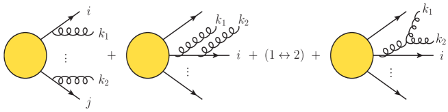
Figure 34: Double soft gluon emission from a generic hard amplitude.

The analysis performed for virtual corrections, leading to the conclusion that soft emissions can be described by means Wilson lines, makes us confident that the simple argument leading to Eq. (6.2), and to the identification of the single soft emission operator in Eq. (6.8), will generalise to the emission of multiple soft gluons at leading power. Indeed, the limit of QCD tree-amplitudes when two gluons become simultaneously soft was studied by Berends and Giele [515] and by Catani [551], showing precisely a factorisation of this kind. Following Ref. [529], we introduce the double-soft emission current by writing

$$\langle a_{1}a_{2}|\otimes\langle\lambda_{1}\lambda_{2}\left|\smash{\mathcal{A}_{\,gg,f_{1}\ldots f_{n}}(k_{1},k_{2},p_{1},\dots,p_{n})}{\vphantom{1}}\right\rangle_{\rm soft}\,=\,\epsilon^{\mu_{1}}_{\lambda_{1}}(k_{1})\epsilon^{\mu_{2}}_{\lambda_{2}}(k_{2})$$

$$\hskip 142.26378pt\times\,J^{a_{1}a_{2}}_{\mu_{1}\mu_{2}}(k_{1},k_{2})\left|\smash{\mathcal{A}_{\,f_{1},\dots,f_{n}}(p_{1},\dots,p_{n})}{\vphantom{1}}\right\rangle\,.$$ (6.9)

The double-soft current receives contribution from three different diagram topologies, depicted in Fig. 34. The explicit expression for the double-soft current $J_{a_{1}a_{2}}^{\mu_{1}\mu_{2}}$ is given by [529]

$$J^{a_{1}a_{2}}_{\mu_{1}\mu_{2}}(k_{1},k_{2}) = 4\pi\alpha_{s}\mu^{2\epsilon}\Bigg{\{}\sum_{\ell\neq m}T_{m}^{a_{1}}\,T_{\ell}^{a_{2}}\,\frac{p_{m}^{\mu_{1}}}{p_{m}\cdot k_{1}}\,\frac{p_{\ell}^{\mu_{2}}}{p_{\ell}\cdot k_{2}}$$

$$\hskip 28.45274pt+\,\sum_{m}\,\bigg{[}\,\frac{p_{m}^{\mu_{1}}\,p_{m}^{\mu_{2}}}{p_{m}\cdot\left(k_{1}+k_{2}\right)}\left(\frac{T_{m}^{a_{2}}T_{m}^{a_{1}}}{p_{m}\cdot k_{2}}\,+\,\left(1\leftrightarrow 2\right)\right)$$

$$\hskip 28.45274pt+\,\,{\rm i}f^{\,\,\,a_{1}a_{2}}_{a}\,T_{m}^{a}\,\,\frac{p_{m}\cdot\left(k_{2}-k_{1}\right)g^{\mu_{1}\mu_{2}}+2\,p_{m}^{\mu_{1}}\,k_{1}^{\mu_{2}}-2\,p_{m}^{\mu_{2}}\,k_{2}^{\mu_{1}}}{2k_{1}\cdot k_{2}\,p_{m}\cdot\left(k_{1}+k_{2}\right)}\bigg{]}\Bigg{\}}\,.$$

The correspondence between the expression in Eq. (6.1) and the diagrams in Fig. 34 is straightforward: the first term stems from diagrams of type (a), the second contribution reflects diagrams of type (b), and finally the last term, proportional to $f_{a}^{\;\;a_{1},a_{2}}$, clearly emerges from diagrams of type (c). At squared-amplitude level, the factorisation formula for the configuration at hand can be written as

$$\Big{|}\mathcal{A}_{\,gg,f_{1}\ldots f_{n}}(k_{1},k_{2},p_{1},l\dots,p_{n})\Big{|}^{2}_{\rm soft}\,=\,2\left(4\pi\alpha_{s}\mu^{2\epsilon}\right)^{2}$$ (6.11)

$$\qquad\times\,\Bigg{[}\sum_{i\neq j}\sum_{k\neq l}\,\mathcal{I}_{ij}^{(1)}\,\mathcal{I}_{kl}^{(2)}\,\Big{|}\mathcal{A}_{\,f_{1}\ldots f_{n}}^{ijkl}(p_{1},\dots,p_{n})\Big{|}^{2}+\sum_{i\neq j}\,\mathcal{I}_{ij}^{(12)}\Big{|}\mathcal{A}_{\,f_{1}\ldots f_{n}}^{ij}(p_{1},\dots,p_{n})\Big{|}^{2}\Bigg{]}\,,$$

where the first term in square brackets is the factorised contribution, proportional to the double-colour-connected matrix element

$$\big{|}\mathcal{A}_{\,f_{1}\ldots f_{n}}^{ijkl}\Big{|}^{2}\,\equiv\,\left\langle\smash{\mathcal{A}_{\,f_{1}\ldots f_{n}}}{\vphantom{1}}\right|\Big{\{}{\bf T}^{i}\cdot{\bf T}^{j},{\bf T}^{k}\cdot{\bf T}^{l}\Big{\}}\left|\smash{\mathcal{A}_{\,f_{1}\ldots f_{n}}}{\vphantom{1}}\right\rangle\,,$$ (6.12)

while the double emission from a single colour dipole si expressed by the kernel $\mathcal{I}_{ij}^{(12)}$, which can be read off from Eq.(109) in [529], after appropriate relabelling of the momenta.

As before, the double-soft current can be extracted from a matrix element of Wilson lines: quite naturally, we propose

$${\cal S}_{\,n,\,2}\big{(}k_{1},k_{2};\{\beta_{i}\}\big{)}\,\equiv\,\left\langle\smash{k_{1},\lambda_{1};k_{2},\lambda_{2}}{\vphantom{1}}\right|\,T\bigg{[}\prod_{i=1}^{n}\Phi_{\beta_{i}}(0,\infty)\bigg{]}\left|\smash{0}{\vphantom{1}}\right\rangle\,.$$ (6.13)

It is straightforward to show that Eq. (6.13), evaluated at tree level, indeed reproduces the current $J^{a_{1}a_{2}}_{\mu_{1}\mu_{2}}$, contracted with gluon polarisation vectors as in Eq. (6.9). Indeed, expanding the product of Wilson lines to order $g^{2}$, there are three different configurations that return non-vanishing contributions: one may expand to first order in $g$ two of the $n$ Wilson lines, obtaining the first term in Eq. (6.1), or one may expand only one Wilson line to order $g$, and then include a Lagrangian interaction, to get the non-abelian component; finally, one can expand a single line up to order $g^{2}$: in this case, the path ordering that defines $\Phi(0,\infty)$ precisely returns the remaining contributions in the first line of Eq. (6.1).

It is important to stress that the singular soft configurations we have just described have been extracted by taking the two soft momenta to vanish at the same rate, formally replacing $k_{1}\to\lambda k_{1}$ and $k_{2}\to\lambda k_{2}$, taking $\lambda\to 0$ and retaining the leading power in $\lambda$. This we describe as a democratic IR limit. In the context of subtraction, as we will see, it is also important to identify hierarchical, or strongly-ordered limits, corresponding to configurations where one gluon is much softer than the other, i.e. one of the two momenta vanishes at a faster rate with respect to the other. The expression of the corresponding current can be easily deduced by taking the leading term in the $k_{1}$ ($k_{2}$) expansion of $J_{a_{1}a_{2}}^{\mu_{1}\mu_{2}}$ at amplitude level, and of $\mathcal{I}_{cd}^{(12)}$ at cross-section level. One gets

$$\big{(}J^{\,\rm s.o.}\big{)}^{a_{1}a_{2}}_{\mu_{1}\mu_{2}}(k_{1},k_{2})\! = \!g_{s}\mu^{\epsilon}\Bigg{(}\sum_{m=1}^{n}T^{a_{2}}_{m}\,\frac{p_{m,\,\mu_{2}}}{p_{m}\cdot k_{2}}\,\delta^{a_{1}a}+{\rm i}\,f^{a_{1}a_{2}a}\,\frac{k_{1,\,\mu_{2}}}{k_{1}\cdot k_{2}}\Bigg{)}\sum_{\ell=1}^{n}\,T_{\ell,\,a}\,\frac{p_{\ell,\,\mu_{1}}}{p_{\ell}\cdot k_{1}}\,,$$

$$\mathcal{I}_{ij}^{(12)\,{\rm s.o.}}\! = \!-2C_{A}\,\mathcal{I}_{ij}^{(2)}\;\Big{[}\mathcal{I}_{i2}^{(1)}+\mathcal{I}_{j2}^{(1)}-\mathcal{I}_{ij}^{(1)}\Big{]}\,.$$ (6.14)

For the purposes of constructing subtraction counterterms in a systematic way, it would be interesting to be able to derive strongly ordered limits in terms of matrix elements of Wilson lines, as done above for the democratic case. This approach will be briefly discussed in Section 6.4. To conclude our discussion of soft factorisations for real radiation at tree level, we recall that the eikonal approximation is spin-independent, so the formulas that we have described can be applied to soft gluon radiation from hard gluons, simply by placing the colour generators in the appropriate (adjoint) representation; furthermore, the case of massless quark radiation (through an intermediate gluon which splits into a quark-antiquark pair) can be treated similarly and does not present new difficulties. We remark also that the soft factorisation is quasi complete, as noted at the beginning of this Section, in the sense that eikonal kernels and Born-like matrix elements are not entirely independent of each other, but are still connected by colour correlations.

To complete the picture of tree-level infrared factorisation for real radiation, we must consider collinear splittings as well. In this case, we will also find a quasi complete factorisation, but with colour correlations replaced by spin correlations. The trivial colour structure of tree-level collinear factorisation is best displayed by picking the most suitable colour basis: in this case, a natural choice is the colour trace basis of Ref. [517], later extensively employed at loop level [552, 521]. For multi-gluon amplitudes, this organisation is intuitively motivated by string theory, where tree-level gluon amplitudes are computed as expectation values of conformal vertex operators inserted on the boundaries of the tree-level string world sheet, which can be conformally mapped to a circle. Colour degrees of freedom are carried by Chan-Paton factors, which are generators for the fundamental representation of the gauge group associated with each external state. The full tree-level amplitude is then constructed as a sum of sub-amplitudes, each corresponding to a cyclic ordering of the vertex operators on the boundary of the circle, and each accompanied by the corresponding trace of Chan-Paton factors. For $n$ gluons, one may write

$${\cal A}_{n}^{a_{1}\ldots a_{n}}(p_{1},\ldots,p_{n})\,=\,\sum_{\sigma\in S_{n}/Z_{n}}{\rm Tr}\Big{[}T^{a_{\sigma(1)}}\ldots T^{a_{\sigma(n)}}\Big{]}\,A_{n}\left(p_{\sigma(1)},\ldots,p_{\sigma(n)}\right)\,,$$ (6.15)

where the sum is over $(n-1)!$ non-cyclic permutations of the $n$ external gluons, and we omitted polarisation indices for simplicity. This string-inspired organisation of gauge amplitudes can be generalised to loop amplitudes, where at $\ell$ loops one must allow for products of up to $\ell+1$ trace factors, and to amplitudes with massless fermions.

The sub-amplitudes $A_{n}$ are gauge invariant, and they enjoy a number of properties that make them very useful for practical calculations [517]. In the present context, the most notable aspect is the fact that, for each sub-amplitude, collinear poles arise only from configurations where the two particles that become collinear are adjacent in the selected cyclic ordering. Thus, for example, $A_{5}(p_{1},p_{2},p_{3},p_{4},p_{5})$ will have a collinear pole when $p_{2}$ becomes collinear to $p_{3}$, but not when $p_{2}$ becomes collinear to $p_{5}$: indeed, within the set of diagrams contributing to this ordering, there is no diagram where $p_{2}$ and $p_{5}$ emerge from the same internal vertex, so that no propagator becomes singular as $p_{2}$ becomes parallel to $p_{5}$. Picking then a sub-amplitude where two momenta $p_{i}$ and $p_{j}$ are adjacent, and the corresponding gluons carry helicities $s_{i}$ and $s_{j}$, one finds that, in the collinear limit, the sub-amplitude factorises as

$$A_{n}^{\,\ldots s_{i}s_{j}\ldots}(\ldots,p_{i},p_{j},\ldots)\Big{|}_{p_{i}||\,p_{j}}\,=\,\sum_{s=\pm}{\rm Split}_{-s}^{(0)}(p_{i},s_{i};p_{j},s_{j})\,A_{n-1}^{\,\ldots s\ldots}(\ldots,p_{i}+p_{j},\ldots)$$ (6.16)

where the parent gluon carrying momentum $p_{i}+p_{j}$ is taken to carry outgoing helicity $(+s)$, so that it enters the tree-level splitting amplitude Split${}_{-s}^{(0)}$ with incoming helicity $(-s)$. The factorisation in Eq. (6.16) encodes the singular behavior of $A_{n}$ as $s_{ij}=2p_{i}\cdot p_{j}\to 0$, which turns out to be proportional to $s_{ij}^{-1/2}$ (giving the expected $1/s_{ij}$ singularity at cross-section level). Tree-level splitting amplitudes in this basis were derived in [514] and in  [517], and are listed in those references for all flavour and spin pairings consistent with QCD couplings. As an example, one can write the splitting amplitude for a gluon branching into two gluons as [530, 534]

$${\rm Split}_{-s}^{(0)}(p_{i},s_{i};p_{j},s_{j})\! = \!g\mu^{\epsilon}\,\frac{2}{s_{ij}}\,\Big{[}\epsilon_{s_{i}}(p_{i})\cdot\epsilon_{s_{j}}(p_{j})\,\,p_{i}\cdot\epsilon_{s}(p_{i}+p_{j})$$

$$+\,\epsilon_{s_{i}}(p_{i})\cdot\epsilon_{s}(p_{i}+p_{j})\,\,p_{i}\cdot\epsilon_{s_{j}}(p_{j})\,-\,\epsilon_{s_{j}}(p_{j})\cdot\epsilon_{s}(p_{i}+p_{j})\,\,p_{j}\cdot\epsilon_{s_{i}}(p_{i})\Big{]}\,,$$

where the parent gluon is taken on shell (i.e. in the exact collinear limit), and the $1/s_{ij}$ singularity is softened to a square root by the products of polarisation vectors in square brackets.

If one does not wish to be constrained by the choice of a specific colour basis, it is possible to rephrase the collinear factorisation of massless multi-particle amplitudes in terms of colour operators (which can then be evaluated in any basis), as was done for soft emissions. In this case, one can write the tree-level factorisation directly in colour space as

$$\left|\smash{\,\mathcal{A}^{\ldots s_{i}s_{j}\ldots}_{n}(\ldots,p_{i},p_{j},\ldots)}{\vphantom{1}}\right\rangle_{p_{i}||p_{j}}\,=\,{\bf Sp}^{(0)}_{-s}(p_{i},s_{i};p_{j},s_{j})\left|\smash{\mathcal{A}^{\ldots s\ldots}_{n-1}(\ldots,p_{i}+p_{j},\ldots)}{\vphantom{1}}\right\rangle\,,$$ (6.18)

where the splitting matrix ${\bf Sp}^{(0)}_{-s}$ is now a colour operator acting on the right on the colour index of the parent particle, and on the left on the colour indices of the collinear pair. At tree level, the relation between the operator ${\bf Sp}^{(0)}_{-s}$ and the colourless splitting amplitude Split${}_{-s}^{(0)}$ is trivial, since each possible flavour splitting can be proportional to only a single colour tensor. Thus, for example, for a gluon with colour index $a$ splitting into gluons with colour indices $b$ and $c$, the splitting operator is obtained from Eq. (6.1) by simply inserting a factor of $(-{\rm i}f_{abc})$. More complicated colour structures will, of course, arise for multiple collinear splittings at tree and loop level.

To discuss collinear factorisation at cross-section level, taking into account the non-trivial spin structure, it is useful to define a squared amplitude that is summed over all the spin indices, except for those of a select particle of flavour $f_{1}$, which will be interpreted as the parent particle in the subsequent collinear splitting. Following Ref. [529], we define

$$\mathcal{T}_{\,f_{1}\dots f_{n}}^{\,s_{1}s^{\prime}_{1}}(p_{1},\ldots,p_{n})\,=\,\sum_{s_{2},\ldots,s_{n}}\sum_{c_{i}}\mathcal{A}_{\,f_{1}\ldots f_{n}}^{\,c_{1}\ldots c_{n};\,s_{1}\ldots s_{n}}(p_{1},\dots,p_{n})\Big{[}\mathcal{A}_{\,f_{1}\ldots f_{n}}^{\,c_{1}\dots c_{n};\,s^{\prime}_{1}\ldots s_{n}}(p_{1},\dots,p_{n})\Big{]}^{\dagger}\,.$$ (6.19)

Next, we need to be more precise in parametrising the collinear limit. For two particles of flavour $f_{i}$ and $f_{j}$, carrying momenta $p_{i}$ and $p_{j}$, we identify a light-like momentum $p^{\mu}$ as the collinear direction, and we pick an auxiliary light-like vector $n^{\mu}$. How the collinear direction is approached is specified by the transverse momentum vector $k^{\mu}_{\bot}$, by definition orthogonal to both $p^{\mu}$ and $n^{\mu}$. Each collinear parton carries a collinear momentum fraction which can be defined by $z_{a}=s_{an}/(s_{in}+s_{jn})$, with $a=i,j$ and $s_{an}=2p_{a}\cdot n$, so that $z_{i}+z_{j}=1$; hence, one may use $z\equiv z_{i}$ and $z_{j}=1-z$. This results in the Sudakov parametrisation

$$p_{i}\,=\,z\,p^{\mu}+k_{\bot}^{\mu}-\frac{k_{\bot}^{2}}{z}\,\frac{n^{\mu}}{2p\cdot n}\,,\quad\!p_{j}\,=\,(1-z)\,p^{\mu}-k_{\bot}-\frac{k_{\bot}^{2}}{1-z}\,\frac{n^{\mu}}{2p\cdot n}\,,\quad\!s_{ij}\,=\,-\frac{k_{\bot}^{2}}{z(1-z)}\,.$$ (6.20)

The collinear limit is approached as $k_{\bot}\rightarrow 0$, and the leading-power behaviour of the squared matrix element is encoded by [529]

$$\Big{|}\mathcal{A}_{\,f_{1}\ldots f_{n}}(p_{1},\dots,p_{n})\Big{|}^{2}_{p_{i}||p_{j}}\,=\,\frac{8\pi\alpha_{s}\mu^{2\epsilon}}{s_{ij}}\,\,\mathcal{T}^{ss^{\prime}}_{f,f_{1}\ldots f_{n}}(p,p_{1},\ldots,p_{n})\,\widehat{P}_{f_{i}f_{j}}^{\,ss^{\prime}}\big{(}z,k_{\bot};\epsilon\big{)}\,,$$ (6.21)

where on the r.h.s. it is understood that particles $f_{i}$ and $f_{j}$, carrying momenta $p_{i}$ and $p_{j}$, are omitted from the list, and they have been replaced by a single particle $f$ carrying momentum $p$. The possible flavour combinations are determined by the Feynman rules of the theory under consideration. For QCD, the kernels $\widehat{P}_{a_{i}a_{j}}^{ss^{\prime}}$ are the $d$-dimensional DGLAP splitting functions, represented as spin operators acting on the spin indices $s,s^{\prime}$ of the spin tensor $\mathcal{T}$. The splitting functions are given by squares of the splitting amplitudes ${\bf Sp}^{(0)}_{-s}$, summed over colours, after extracting the coupling and the factor of $1/\sqrt{s_{ij}}$. Their explicit expressions are of course well known, and in the present normalisation they are given by

$$\widehat{P}_{qg}^{ss^{\prime}}(z,k_{\bot};\epsilon)\! = \!\delta_{ss^{\prime}}\,C_{F}\bigg{[}\frac{1+z^{2}}{1-z}-\epsilon(1-z)\bigg{]}\,,$$

$$\widehat{P}_{gq}^{ss^{\prime}}(z,k_{\bot};\epsilon)\! = \!\delta_{ss^{\prime}}\,C_{F}\bigg{[}\frac{1+(1-z)^{2}}{z}-\epsilon z\bigg{]}\,,$$ (6.22)

$$\widehat{P}_{q\bar{q}}^{\mu\nu}(z,k_{\bot};\epsilon)\! = \!T_{R}\bigg{[}-g^{\mu\nu}+4z(1-z)\frac{k_{\bot}^{\mu}k_{\bot}^{\nu}}{k_{\bot}^{2}}\bigg{]}\,,$$

$$\widehat{P}_{gg}^{\mu\nu}(z,k_{\bot};\epsilon)\! = \!2C_{A}\bigg{[}-g^{\mu\nu}\Big{(}\frac{z}{1-z}+\frac{1-z}{z}\Big{)}-2(1-\epsilon)z(1-z)\frac{k_{\bot}^{\mu}k_{\bot}^{\nu}}{k_{\bot}^{2}}\bigg{]}\,.$$

Notice that all the kernels are symmetric under the exchange of a quark with an anti-quark, i.e. $\widehat{P}_{Xq}=\widehat{P}_{X\bar{q}}$. From Eq. (6.1) it is evident that the spin sensitivity of the kernels, and, consequently, the one of the spin tensor, is trivial in the case of a parent fermion, while gluon splittings retain a non-trivial azimuthal dependence. Also in the collinear sector, we are interested in expressing the singular kernels in terms of universal, gauge invariant operators. Let us begin by by considering gluon radiation from an outgoing quark: in this case, we may take inspiration from the virtual jet function defined in Eq. (4.9), and implement collinear radiation, as was done for the soft current, by including an extra gluon in the final state. At amplitude level, this amounts to introducing the matrix element

$$\overline{u}_{s}(p){\cal J}_{q,\,1}^{\lambda}\big{(}k;p,n\big{)}\,\equiv\,\left\langle\smash{p,s;k,\lambda}{\vphantom{1}}\right|\,T\Big{[}\Phi_{n}(\infty,0)\,\psi(0)\Big{]}\left|\smash{0}{\vphantom{1}}\right\rangle\,.$$ (6.23)

The function ${\cal J}_{q,\,1}^{\lambda}$ is a spin matrix, and at tree level it must reproduce the collinear singularity of the splitting amplitudes, stripped of colour information. The dependence on the vector $n^{\mu}$ defining the Wilson line mimicks the gauge dependence within the families of axial gauges, and choosing $n^{2}=0$ one can reproduce the Sudakov parametrisation of the collinear region. To test our ansatz, we can square Eq. (6.23), take a Fourier transform, and introduce the (unpolarised) cross-section-level radiative jet function

$$J_{q,\,1}\big{(}k;l,p,n\big{)}\equiv\int d^{d}x\,{\rm e}^{{\rm i}l\cdot x}\,\sum_{\lambda,s}\left\langle\smash{0}{\vphantom{1}}\right|\,T\,\Big{[}\Phi_{n}(\infty,x)\,\psi(x)\Big{]}\left|\smash{p,s;k,\lambda}{\vphantom{1}}\right\rangle$$

$$\hskip 85.35826pt\times\,\left\langle\smash{p,s;k,\lambda}{\vphantom{1}}\right|\,\overline{T}\,\Big{[}\overline{\psi}(0)\,\Phi_{n}(0,\infty)\Big{]}\left|\smash{0}{\vphantom{1}}\right\rangle\,,$$ (6.24)

where the complex-conjugate matrix element is anti-time-ordered by the action of the operator $\overline{T}$, and the vector $l^{\mu}$ plays the role of the total momentum flowing into the final state. We can now perform a simple test of the correctness of our assumptions by computing, in Feynman gauge, the lowest perturbative order for Eq. (6.1). It receives contributions from three different Feynman diagrams, displayed in Fig. 35.

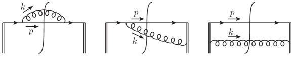
Figure 35: Feynman graphs contributing to the radiative quark jet function, defined in Eq. (6.1), at lowest order.

Taking, for simplicity, $n^{2}=0$, we find

$$J_{q,\,1}^{(0)}\big{(}k;l,p,n\big{)}\,=\,\frac{4\pi\alpha_{s}}{(l^{2})^{2}}\,C_{F}\,(2\pi)^{d}\delta^{d}\left(l-p-k\right)\left[-l\hskip-4.49997pt/\gamma_{\mu}p\hskip-4.49997pt/\gamma^{\mu}l\hskip-4.49997pt/+\frac{l^{2}}{k\cdot n}\big{(}\,l\hskip-4.49997pt/n\hskip-4.49997pt/p\hskip-4.49997pt/+p\hskip-4.49997pt/n\hskip-4.49997pt/l\hskip-4.49997pt/\,\big{)}\right]\,.$$ (6.25)

It is easy to verify the correspondence between the contributions of the three diagrams in Fig. 35 and the axial-gauge calculation of tree-level splitting kernel in Ref. [529]. Notice however that in Eq. (6.25) the collinear limit for $k$ and $p$, corresponding to $l^{2}\to 0$, still has to be performed. This can be done exploiting the Sudakov parametrisation in Eq. (6.20), and truncating the expressions for the two collinear momenta at leading order in the transverse momentum, as

$$p^{\mu}\,=\,zl^{\mu}+{\cal O}\left(l_{\perp}\right)\,,\qquad k^{\mu}\,=\,(1-z)l^{\mu}+{\cal O}\left(l_{\perp}\right)\,,\qquad n^{2}\,=\,0\,.$$ (6.26)

At leading power in $l_{\bot}$ we easily find

$$J_{q,\,1}^{(0)}\big{(}k;l,p,n\big{)}\,=\,\frac{8\pi\alpha_{s}}{l^{2}}\,C_{F}\,(2\pi)^{d}\,\delta^{d}\left(l-p-k\right)\,l\hskip-4.49997pt/\,\left[\frac{1+z^{2}}{1-z}-\epsilon\left(1-z\right)\right]\,,$$ (6.27)

up to corrections of relative order $l_{\bot}^{2}$. In the square bracket, as expected, we recognise the leading order unpolarised DGLAP splitting function $P_{qg}$, as reported in Eq. (6.1).

Clearly, the number and complexity of splitting functions at amplitude and cross-section level rapidly increases at higher orders, both because loop corrections must be included, and because multiple real radiation comes into play; furthermore, when multiple collinear particles are radiated, the identification of strongly-ordered limits becomes relevant. The operator matrix element expressions that we have identified in these simple examples, however, point the way to a useful systematic approach, linking together virtual corrections and real radiation. We will now proceed by first introducing the problem of infrared subtraction is some detail, and then discussing a set of possible definitions for real-radiation soft and collinear counterterms to all orders in perturbation theory.

6.2 Introducing the problem of infrared subtraction at NLO

The discussion in Section 6.1 lays the groundwork for constructing a practical and general implementation of the cancellation of IR divergences in IR-safe observables, which follows from the KLN theorem discussed in Section 1.2. After our discussion of the general cancellation theorems, and our tour of many technical aspects of IR factorisation, the reader may well wonder why this cancellation should still be described as a ‘problem’. Indeed, so long as one is computing total cross sections, or highly inclusive observables, the cancellation between divergences coming from virtual corrections and those stemming from the phase space integration of unresolved radiation can be performed analytically, even to rather high orders in perturbation theory. What changes the game, and raises the stakes, is the nature of typical collider observables. Even the definition of IR-safe observables, and verifying their IR-safety to all orders, become non-trivial questions. Experimental observables are very often defined in terms of particle jets, and jets in turn are typically defined in terms of clustering algorithms; furthermore, experimental constraints imply complex phase space cuts on kinematic variables, often arising at the level of triggers for data collection: these must be implemented in efficient and versatile numerical codes. In practice, this means that phase-space integrals of real-radiation matrix elements must be performed numerically, and this in turn requires subtracting their singular contributions before performing the integration in $d=4$. Another way to state the problem is that, in a collider environment, versatility means being able to provide fully differential distribution for interesting observables, in order to be able to cope with different sets of experimental cuts. As a consequence, it becomes necessary to perform the extraction of singular contributions in a universal way, for arbitrary configurations of the resolved particles. The factorisation properties of real radiation matrix elements, sketched in Section 6.1, suggest that completing this program is possible in principle, however a general and efficient practical implementation at high orders is far from easy to achieve.

In this section, we will present the basic ideas that have been applied to the cancellation problem, in the relatively simple context of NLO calculations, where, arguably, the problem is satisfactorily solved. In the past decades, two main strategies have been developed to solve the problem at NLO: the slicing [553, 554, 555] approach and the subtraction [80, 556, 81, 557, 558, 559] approach. In what follows, we will mainly develop the subtraction viewpoint, but, in order to present the basic idea behind these methods, we illustrate them in the context of a toy model. Start by considering the integral

$$I(F)\,=\,\lim_{\epsilon\rightarrow 0}\Bigg{[}\int_{0}^{1}\frac{dx}{x}\,x^{\epsilon}\,F(x)-\frac{1}{\epsilon}\,F(0)\Bigg{]}\,,$$ (6.28)

where $F(x)$ is a generic function admitting a Taylor expansion around $x=0$, and the first term mimicks the phase-space integration of the real radiation, while the second term plays the role of the virtual correction. The goal of both slicing and subtraction schemes is computing $I(F)$ without relying on the analytic evaluation of the integral over $x$, which involves the arbitrarily complicated function $F$. The slicing approach tackles the problem by splitting the integration domain by means of a small parameter $\delta\ll 1$, and working with a simple approximate expression for $F$ (for example $F(0)$) in the region containing the singularity. One writes then

$$I(F)\simeq\lim_{\epsilon\rightarrow 0}\Bigg{[}\,F(0)\int_{0}^{\delta}\frac{dx}{x}\,x^{\epsilon}+\int_{\delta}^{1}\frac{dx}{x}\,x^{\epsilon}\,F(x)-\frac{1}{\epsilon}\,F(0)\Bigg{]}\,=\,F(0)\,\log\delta+\int_{\delta}^{1}\frac{dx}{x}\,x^{\epsilon}\,F(x)\,.$$ (6.29)

The r.h.s. of Eq. (6.29) is manifestly finite as $\epsilon\to 0$, and therefore is suitable for numerical evaluation. The slicing procedure is simple and intuitive, but of course, depending on the required accuracy, one needs to worry about the residual dependence on the slicing parameter $\delta$, which needs to be small, but not too small. The problem is not insurmountable, and can be significantly ameliorated by improving the estimate for $F(x)$ to be employed in the singular region (see, for example, [560, 561]).

To avoid problems associated with the sensitivity to the slicing parameter, the subtraction approach proceeds by subtracting from $F(x)$ its value in $x=0$, and adding it back in integrated form, therefore leaving $I(F)$ unchanged. In formulae

$$I(F)\,=\,\lim_{\epsilon\rightarrow 0}\Bigg{[}\int_{0}^{1}\frac{dx}{x}\,x^{\epsilon}\Big{(}F(x)-F(0)\Big{)}+\int_{0}^{1}\frac{dx}{x}\,x^{\epsilon}\,F(0)-\frac{1}{\epsilon}\,F(0)\Bigg{]}\,.$$ (6.30)

Once again, the first term is finite in $\epsilon$ by construction, while the proposal is to evaluate the second one analytically to cancel the explicit pole of the last term. This is of course trivial in this toy example, but requires considerable care in realistic calculations, as we will see. Let us stress that no approximations have been made to write Eq. (6.30). At NLO, the subtraction schemes proposed by Catani and Seymour in [81], and by Frixione, Kunszt and Signer in [80] have been fully developed for general collider processes, and both are implemented in efficient event generators [562, 563, 564, 565, 566, 559]. One can argue that the IR subtraction problem can be considered solved in full generality at this accuracy.

Before moving on to higher orders, let us introduce some notation, in order to describe the subtraction approach more precisely. Let us consider, for simplicity a production process involving $n$ massless final-state coloured particles at Born level, and let $\mathcal{A}_{n}(p_{i})$, $i=1,\ldots,n$, be the relevant scattering amplitude. We expand the amplitude in perturbation theory as

$${\cal A}_{n}(p_{i})\,=\,{\cal A}_{n}^{(0)}(p_{i})\,+\,{\cal A}_{n}^{(1)}(p_{i})\,+\,{\cal A}_{n}^{(2)}(p_{i})\,+\,\ldots\,,$$ (6.31)

where $\mathcal{A}_{n}^{(k)}$ is the $k$-loop correction, including the appropriate power of the strong coupling constant. Moreover, consider a generic infrared-safe observable $X$, whose differential distribution is given by

$$\frac{d\sigma}{dX}\,=\,\frac{d\sigma_{\mbox{\tiny{LO}}}}{dX}\,+\,\frac{d\sigma_{\mbox{\tiny{NLO}}}}{dX}\,+\,\frac{d\sigma_{\mbox{\tiny{NNLO}}}}{dX}\,+\,\ldots\,.$$ (6.32)

The leading-order contribution is proportional to the Born transition probability, $B_{n}\,\equiv\,\big{|}{\cal A}_{n}^{(0)}\big{|}^{2}$, and is IR finite. Starting with NLO, the infrared content of the distribution becomes relevant, and $d\sigma/dX$ must be computed by combining unresolved radiative contributions with loop corrections. Writing

$$R_{n+1}\,\equiv\,\left|{\cal A}_{n+1}^{(0)}\right|^{2}\,,\qquad V_{n}\,=\,2{\bf Re}\left[{\cal A}_{n}^{(0){\dagger}}\,{\cal A}_{n}^{(1)}\right]\,,$$ (6.33)

we know that infrared poles in $V_{n}$ will be cancelled by the integration of unresolved radiation in $R_{n+1}$. At this stage, therefore, both contributions must be regulated, and we write the NLO distribution as

$$\frac{d\sigma_{\mbox{\tiny{NLO}}}}{dX} = \lim_{d\to 4}\Bigg{\{}\!\int d\Phi_{n}\,V_{n}\,\delta_{n}(X)+\int d\Phi_{n+1}\,R_{n+1}\,\delta_{n+1}(X)\Bigg{\}}\,,$$ (6.34)

where $\delta_{m}(X)\equiv\delta(X-X_{m})$ fixes $X_{m}$, the expression for the observable appropriate for an $m$-particle configuration, to the prescribed value $X$, and $d\Phi_{m}$ denotes the Lorentz-invariant phase space measure for $m$ massless final state particles.

Following the idea described in Eq. (6.30), we introduce a local counterterm $K_{n+1}^{\,(\mathbf{1})}$, which is required to mimic the singular IR behaviour of the real-radiation matrix element locally in phase space, and, at the same time, is expected to be simple enough to be analytically integrated in the radiative phase space $d\Phi_{\rm rad,1}\equiv d\Phi_{{n+1}}/d\Phi_{n}$. If this is possible, one can compute the integrated counterterm

$$I_{n}^{\,({\bf 1})}\,=\,\int d\Phi_{\rm rad,1}\,K_{n+1}^{\,(\mathbf{1})}\,,$$ (6.35)

exposing explicit poles corresponding to the phase space singularities of the integrand, which, in turn, are the same as those of the real-radiation matrix element. It is now possible to construct a version of Eq. (6.34) where virtual corrections and real contributions are separately finite, and therefore phase space integrals can be performed numerically when needed:

$$\frac{d\sigma_{\mbox{\tiny{NLO}}}}{dX}\,=\,\int d\Phi_{n}\Big{[}V_{n}+I_{n}^{\,({\bf 1})}\Big{]}\,\delta_{n}(X)+\int d\Phi_{n+1}\,\Big{[}R_{n+1}\,\delta_{n+1}(X)-K_{n+1}^{\,(\mathbf{1})}\,\delta_{n}(X)\Big{]}\,.$$ (6.36)

The interpretation of Eq.(6.36) is the following: the combination $R_{n+1}-K_{n+1}^{\,(\mathbf{1})}$ is free of phase-space singularities by construction, while $I_{n}$ cancels the explicit poles of the virtual correction, as a direct consequence of the KLN theorem. The sum $V_{n}+I_{n}$ is thus finite as $\epsilon\rightarrow 0$, and both combinations in square brackets are suitable for a numerical implementation. Note that IR safety of the observable $X$ is necessary for the cancellation, which requires $\delta_{n+1}(X)$ to turn smoothly into $\delta_{n}(X)$ in all unresolved limits.

Clearly, the actual definition of an appropriate local counterterm is not unique, and characterises the subtraction scheme. A precise definition must include a prescription to map the phase space for ${n+1}$ massless on-shell particles in the radiative phase space to a configuration of $n$ massless on-shell particles in the Born-level phase space, satisfying the same momentum conservation condition, in order to work at all stages with well-defined matrix elements (see, for example, [567]). Furthermore, care must be taken to include in the counterterm all singular limits of the matrix element, subtracting all possible double countings of soft and collinear regions. To illustrate and clarify the procedure that we have just rather formally described, we now briefly summarise a possible sequence of steps to build a suitable NLO counterterm. More details on the procedure, and on its extension to NNLO, can be found in [568]. We note that the procedure described below is just an example, and a number of alternative strategies exist [82].

In order to isolate and enumerate the singular regions in the radiative phase space, following the logic of [80], we begin by introducing a set of sector functions ${\cal W}_{ij}$, which constitute a partition of unity, and subdivide the phase space in cells where the only singularities are due to a selected particle $i$ becoming soft, or becoming collinear to a second particle $j$. As an example, following [568], define

$$e_{i}\,\equiv\,\frac{s_{qi}}{s}\,,\qquad w_{ij}\,\equiv\,\frac{ss_{ij}}{s_{qi}s_{qj}}\,,\qquad\sigma_{ij}\,\equiv\,\frac{1}{e_{i}w_{ij}}\,,$$ (6.37)

where, as we are considering final-state coloured particles only, we can work with a fixed total incoming momentum $q^{\mu}$, and we defined $s=q^{2}$ and $s_{q\ell}=2q\cdot p_{\ell}$. In terms of these variables, we can define the sector functions as

$${\cal W}_{ij}\,\equiv\,\frac{\sigma_{ij}}{\sum_{k\neq l}\sigma_{kl}}\,,$$ (6.38)

obviously satisfying $\sum_{i\neq j}{\cal W}_{ij}=1$. Next, we introduce two operators, ${\bf S}_{i}$ and ${\bf C}_{ij}$, which are defined to extract from the functions on which they act the leading power in the Laurent expansion in the normal variables defining the soft and collinear singularities, respectively. Thus, for example, the action of ${\bf S}_{i}$ on the real radiation matrix element $R_{n+1}$ yields Eq. (6.5), upon identifying particle $i$ with the gluon of momentum $k$; similarly, the action of ${\bf C}_{ij}$ on $R_{n+1}$ yields Eq. (6.21). Acting on the sector functions ${\cal W}_{ij}$, the operators satisfy

$${\bf S}_{i}\sum_{k\neq i}{\cal W}_{ik}\,=\,1\,,\qquad{\bf C}_{ij}\Big{[}{\cal W}_{ij}+{\cal W}_{ji}\Big{]}\,=\,1\,.$$ (6.39)

One easily verifies that the function $R_{n+1}{\cal W}_{ij}$ is only singular when particle $i$ becomes soft and when the pair $ij$ becomes collinear; Eq. (6.39) then guarantees that, upon suitably summing over sectors, the full soft and collinear singularities are recovered, and sector functions will not explicitly appear in the soft and collinear counterterms that will need to be integrated.

At this stage, we can construct a candidate counterterm, by taking the combination

$$K^{({\bf 1})}_{n+1}\,=\,\sum_{i}\sum_{j\neq i}\Big{(}{\bf S}_{i}+{\bf C}_{ij}-{\bf S}_{i}{\bf C}_{ij}\Big{)}R_{n+1}{\cal W}_{ij}\,,$$ (6.40)

where the last term in parentheses subtracts the soft-collinear regions, which would otherwise be doubly counted. Note that this requires that the operators ${\bf S}_{i}$ and ${\bf C}_{ij}$ be defined to commute. We describe Eq. (6.40) as a candidate counterterm because it is not quite ready to be used directly in Eq. (6.36). The reason can be traced to the definition of the integrated counterterm $I_{n}^{({\bf 1})}$ in Eq. (6.35), with its phase-space measure $d\Phi_{{\rm rad},\,1}$. Operationally, in order to perform that integration in a universal, process-independent way, $K^{({\bf 1})}_{n+1}$ must factorise a Born-level squared matrix element involving $n$ on-shell particles, whose momenta must still satisfy the original momentum-conservation condition in the full phase space $d\Phi_{n+1}$: only in this way the definition of $d\Phi_{{\rm rad},\,1}$ makes sense, and the remaining integration in $d\Phi_{n}$ can be performed at a later stage for both terms in Eq. (6.36) without ambiguities. To solve this problem, one needs to provide a mapping of the $({n+1})$-particle phase space onto the $n$-particle phase space, which must not affect soft and collinear limits at leading power. An example of such a mapping is given by [81]

$$\overline{p}_{i}^{(abc)}\,=\,p_{i}\,\,\,\,{\rm if}\,i\neq a,b,c\,;\quad\overline{p}_{b}^{(abc)}\,=\,p_{a}+p_{b}-\frac{s_{ab}}{s_{ac}+s_{bc}}p_{c}\,;\quad\overline{p}_{c}^{(abc)}\,=\,\frac{s_{abc}}{s_{ac}+s_{bc}}p_{c}\,;$$ (6.41)

one easily verifies that the $n$ momenta $\overline{p}_{\ell}^{(abc)}$, with $\ell=1,\ldots,n$, are massless, their sum equals the sum of the original of ${n+1}$ momenta $p_{j}$, with $j=1,\ldots,{n+1}$, and finally the two sets coincide when $p_{a}$ becomes soft and when $p_{a}$ becomes collinear to $p_{b}$. We can now turn our candidate counterterm in Eq. (6.40) into a full-fledged local counterterm, suitable for direct use in Eq. (6.36), by taking the factorised expressions for soft and collinear limits (Eq. (6.5) and Eq. (6.21), respectively) and evaluating the Born-level squared matrix elements on mapped momentum configurations of the form of Eq. (6.41), sector by sector in the radiative phase space. Notice that there is ample freedom in the choice of phase space mappings (see, for example, Ref. [567]), but they are not arbitrary: in particular, taking the limits ${\bf S}_{i}$ and ${\bf C}_{ij}$, or their combinations, on the mapped counterterm, must yield the same result as taking the limits on the candidate counterterm.

Having illustrated in some detail the structure of IR subtraction at NLO, we now discuss in general terms how this structure generalises to higher orders. In Section 6.3, we will see how the factorisation of virtual corrections to scattering amplitudes provides the ingredients for defining soft and collinear candidate counterterms to all orders in perturbation theory. Finally, in Section 6.4 we will discuss the structure of counterterms needed at NNLO.

6.3 Soft and collinear local counterterms: a general strategy

The results of Section 6.1 and Section 6.2 strongly suggest that local infrared counterterms for real radiation should be computable in terms of matrix elements of fields and Wilson lines, which could be easily matched to those expressing infrared virtual corrections, allowing for a transparent cancellation of singularities.

In what follows, we introduce a theoretical framework based on this idea [295]. Using as a guiding principle the factorisation structure of virtual gauge amplitudes, we propose a general definition of local soft and collinear candidate counterterms, valid to all orders in perturbation theory and for any number of real radiated particles. These candidate counterterms can be straightforwardly combined with their virtual counterparts, building up manifestly finite quantities. Of course, candidate counterterms will still need the appropriate phase space mappings to become part of a full-fledged subtraction algorithm.

Inspired by the NLO results in Section 6.1, and in particular by the definitions in Eq. (6.8), Eq. (6.13), and Eq. (6.23), our strategy to define the soft and collinear counterterms can be schematically summarised as follows.

• We introduce radiative soft, collinear and soft-collinear functions at amplitude level, using matrix elements with the same structure as for virtual corrections, but including on-shell real radiation in the final state.

• We square these matrix elements to build cross-section-level radiative soft and jet functions, local in the radiative phase space: these will be our candidate counterterms.

• We show that our candidate counterterms, when summed over the number of radiated particles, and integrated over the corresponding phase spaces, including the case of no radiation, build up quantities that are IR finite to all orders in perturbation theory. This proves that our candidate counterterms, upon integration, will indeed cancel virtual IR poles order by order.

Beginning with soft radiation, consider the case of $n$ hard particles, represented by Wilson lines in the soft approximation, radiating $m$ soft gluons, and introduce the eikonal form factors

$${\cal S}_{n,\,m}\Big{(}\{k_{m}\},\{\beta_{i}\}\Big{)} = \left\langle\smash{k_{1},\lambda_{1};\ldots;k_{m},\lambda_{m}}{\vphantom{1}}\right|\,T\bigg{[}\prod_{i=1}^{n}\Phi_{\beta_{i}}(\infty,0)\bigg{]}\left|\smash{0}{\vphantom{1}}\right\rangle$$ (6.42)

$$= \sum_{p=0}^{\infty}{\cal S}_{n,\,m}^{(p)}\Big{(}\{k_{m}\},\{\beta_{i}\}\Big{)}\,,$$

where the second line defines the perturbative expansion of the matrix element in powers of the coupling $g$. Note that the definition in Eq. (6.42) includes loop corrections to all orders, and can easily be modified to include soft final state fermions, by simply adding them to the list of final state particles. For $m=0$, we recover the definition of the virtual soft function for $n$ particles, given in in Eq. (5.6), while for $m=1,2$ we get Eq. (6.8) and Eq. (6.13). The working assumption behind Eq. (6.42) is that the exact amplitude for the emission of $m$ soft gluons from $n$ hard coloured particles obeys, to all orders, the factorisation

$${\cal A}_{n,\,m}\left(k_{1},\ldots,k_{m};p_{i}\right)\,\simeq\,{\cal S}_{n,\,m}\left(k_{1},\ldots,k_{m};\beta_{i}\right)\,{\cal H}_{n}(p_{i})\,,$$ (6.43)

with corrections that are finite in four dimensions, and integrable in the soft particle phase space. Eq. (6.43) is proven to all orders for $m=0$, and it is consistent with all known perturbative results, in particular with the arguments of [525, 527, 529]. To check the consistency of this approach beyond tree level, one can focus on the case of single soft radiation at one loop, where Eq. (6.43) reads

$${\cal A}_{n,\,1}^{(1)}\left(k;p_{i}\right)\,=\,{\cal S}_{n,\,1}^{(0)}\left(k;\beta_{i}\right)\,{\cal H}^{(1)}_{n}(p_{i})\,+\,{\cal S}_{n,\,1}^{(1)}\left(k;\beta_{i}\right)\,{\cal H}^{(0)}_{n}(p_{i})\,.$$ (6.44)

The first term describes tree-level soft-gluon emission, multiplying the finite part of the one-loop correction to the Born process; the second term has both explicit soft poles and singular factors from single soft real radiation. Eq. (6.44) should be compared with the soft factorisation proposed in [525],

$${\cal A}_{n,\,1}\left(k;p_{i}\right)\,=\,\epsilon^{*\,(\lambda)}(k)\cdot J_{\mbox{\tiny{CG}}}\left(k,\beta_{i}\right)\,{\cal A}_{n}(p_{i})\,,$$ (6.45)

where the Catani-Grazzini soft current $J_{\mbox{\tiny{CG}}}\!\left(k,\beta_{i}\right)$ multiplies the full $n$-particle amplitude, including loop corrections containing infrared poles. In order to map the two calculations, one may express the one-loop hard part ${\cal H}_{n}^{(1)}(p_{i})$ using Eq. (6.43) for $m=0$, with the result

$${\cal H}^{(1)}_{n}(p_{i})\,=\,{\cal A}^{(1)}_{n}\left(p_{i}\right)-{\cal S}^{(1)}_{n}\left(\beta_{i}\right)\,{\cal A}^{(0)}_{n}(p_{i})\,,$$ (6.46)

where we normalised ${\cal S}^{(0)}_{n}$ to the identity operator in colour space. This leads to an expression for the Catani-Grazzini one-loop soft-gluon current in terms of eikonal form factors, as

$$\epsilon^{*\,(\lambda)}(k)\cdot J^{(1)}_{\mbox{\tiny{CG}}}(k,\beta_{i})\,\,\,=\,\,{\cal S}_{n,\,1}^{(1)}\left(k;\beta_{i}\right)\,-\,{\cal S}_{n,\,1}^{(0)}\left(k;\beta_{i}\right)\,{\cal S}^{(1)}_{n}\left(\beta_{i}\right)\,.$$ (6.47)

Comparing Eq. (6.47) with the calculation in [525], one easily recognises that the same combination of Feynman diagrams is involved, and one recovers the known result

$$\left[J^{(1)}_{CG}\right]^{\mu}_{a}(k,\beta_{i}) = -\frac{\alpha_{s}}{4\pi}\,\frac{1}{\epsilon^{2}}\,\frac{\Gamma^{3}(1-\epsilon)\Gamma^{2}(1+\epsilon)}{\Gamma(1-2\epsilon)}$$ (6.48)

$$\times\,{\rm i}f_{a}^{\,\,bc}\sum_{i=1}^{n}\sum_{j\neq i}T_{i}^{b}T_{j}^{c}\left(\frac{\beta_{i}^{\mu}}{\beta_{i}\cdot k}-\frac{\beta_{j}^{\mu}}{\beta_{j}\cdot k}\right)\left[\frac{2\pi\mu^{2}\left(-\beta_{i}\cdot\beta_{j}\right)}{\beta_{i}\cdot k\,\beta_{j}\cdot k}\right]^{\epsilon}\,.$$

For the purposes of subtraction, we now need to build a cross-section-level quantity: the eikonal form factor has to be multiplied times its complex conjugate, and one may perform the (trivial) polarisation sum. The result is the eikonal transition probability

$$S_{n,\,m}\Big{(}\{k_{m}\},\{\beta_{i}\}\Big{)}\,\equiv\,\sum_{p=0}^{\infty}\,S_{n,\,m}^{(p)}\Big{(}\{k_{m}\},\{\beta_{i}\}\Big{)}$$ (6.49)

$$\equiv\,\sum_{\{\lambda_{i}\}}\left\langle\smash{0}{\vphantom{1}}\right|\overline{T}\left[\prod_{i=1}^{n}\Phi_{\beta_{i}}(0,\infty)\right]\left|\smash{k_{1},\lambda_{1};\ldots;k_{m},\lambda_{m}}{\vphantom{1}}\right\rangle\left\langle\smash{k_{1},\lambda_{1};\ldots;k_{m},\lambda_{m}}{\vphantom{1}}\right|T\left[\prod_{i=1}^{n}\Phi_{\beta_{i}}(\infty,0)\right]\left|\smash{0}{\vphantom{1}}\right\rangle\,,$$

where we used again the operator $\overline{T}$, as in Eq. (6.1), and we exploited the Wilson line property that $\Phi^{\dagger}_{n}(a,b)=\Phi_{n}(b,a)$. One could now make use of the completeness of the Fock basis in the soft gluon Hilbert space

$${\bf 1}\,=\,\left|\smash{0}{\vphantom{1}}\right\rangle\left\langle\smash{0}{\vphantom{1}}\right|+\sum_{\ell=1}^{\infty}\bigg{(}\int\prod_{i=1}^{\ell}d\Phi_{1}(k_{i})\bigg{)}\left|\smash{k_{1},\dots,k_{\ell}}{\vphantom{1}}\right\rangle\left\langle\smash{k_{1},\dots,k_{\ell}}{\vphantom{1}}\right|\,,$$ (6.50)

where $d\Phi_{1}(k)=d^{d-1}k/(2k^{0}(2\pi)^{d-1})$, to perform the final-state sum, with the result

$$\sum_{m=0}^{\infty}\int d\Phi_{m}\,S_{n,\,m}\Big{(}\{k_{m}\};\{\beta_{i}\}\Big{)}\,=\,\left\langle\smash{0}{\vphantom{1}}\right|\,\overline{T}\left[\prod_{i=1}^{n}\Phi_{\beta_{i}}(0,\infty)\right]T\left[\prod_{i=1}^{n}\Phi_{\beta_{i}}(\infty,0)\right]\left|\smash{0}{\vphantom{1}}\right\rangle\,.$$ (6.51)

with $d\Phi_{m}=\prod_{i=1}^{m}d\Phi_{1}(k_{i})$. In Eq. (6.51) one recognises an eikonal total cross section, where all the coloured particles belong to the final state. Thanks to the standard cancellation theorems (which can be verified with power-counting arguments), such cross sections are IR finite to all orders in perturbation theory: this implies that the transition probability in Eq. (6.49), which is fully local in the radiation phase space, indeed provides a set of candidate counterterms for soft divergences. Note that, as written, the phase-space sum in Eq. (6.50) will lead to ultraviolet singularities: these can be dealt with by means of a suitable regulator, without affecting infrared poles. Indeed, eikonal cross sections with the general structure of Eq. (6.51) have been extensively used in the past, in the context of the resummation program for threshold and transverse momentum logarithms in QCD (see, for example, [226, 569]) and in SCET [96]: in those cases, one incorporates phase-space constraints by shifting the origin of the Wilson line in the complex-conjugate amplitude, and taking a suitable Fourier transform. In the process, the UV region of the phase-space integral is automatically regulated. These manipulations do not affect the infrared behaviour of the cross section.

We conclude that Eq. (6.51) provides a prescription to cancel virtual poles of soft origin against phase-space integrals of the appropriate set of radiative soft functions, which approximates the relevant squared matrix element at leading power in the soft momenta. For example, we can expand Eq. (6.51) at NLO, obtaining

$$S_{n,\,0}^{(1)}+\int d\Phi_{1}(k)\,S_{n,\,1}^{(0)}(k)\,=\,\text{finite}\,.$$ (6.52)

The first term coincides with the squared virtual function in Eq. (4.8), and therefore contains the same soft poles as the virtual matrix element. The second contribution provides a natural candidate for the integrated countertem.

The collinear component can be handled in analogy to the soft case. Starting from the definition in Eq. (4.9), and generalising along the lines of Eq. (6.23), we introduce amplitude-level radiative jet functions [112, 113, 123, 570, 571] for quark-induced processes, by including in the final state an arbitrary number of outgoing gluons (again, other particles can be included by simply modifying the final-state quantum numbers). We define

$$\overline{u}_{s}(p)\,{\cal J}_{q,\,m}^{\{\lambda_{i}\}}\big{(}\{k_{m}\};p,n\big{)} \equiv \left\langle\smash{p,s;k_{1},\lambda_{1};\ldots;k_{m},\lambda_{m}}{\vphantom{1}}\right|\overline{\psi}(0)\,\Phi_{n}(0,\infty)\left|\smash{0}{\vphantom{1}}\right\rangle$$ (6.53)

$$\equiv \overline{u}_{s}(p)\sum_{p=0}^{\infty}{\cal J}_{q,\,m}^{(p)}\big{(}\{k_{m}\};p,n\big{)}\,,$$

where, again, the second line defines the perturbative expansion of the jet function. At cross-section level, one needs to account for the conservation of the momentum flowing in the final state. To do so, in analogy with what is done for parton distributions, we shift the field position in the complex-conjugate amplitude, and we take a Fourier transform, defining the collinear transition probability as

$$J_{q,\,m}\big{(}\{k_{m}\};l,p,n\big{)}\,\equiv\,\sum_{p=0}^{\infty}J_{q,\,m}^{(p)}\big{(}\{k_{m}\};l,p,n\big{)}$$ (6.54)

$$\equiv\,\int d^{d}x\,{\rm e}^{{\rm i}l\cdot x}\sum_{\{\lambda_{m}\}}\left\langle\smash{0}{\vphantom{1}}\right|\overline{T}\Big{[}\Phi_{n}(\infty,x)\,\psi(x)\Big{]}\left|\smash{p,s;\{k_{m},\lambda_{m}\}}{\vphantom{1}}\right\rangle\left\langle\smash{p,s;\{k_{m},\lambda_{m}\}}{\vphantom{1}}\right|T\Big{[}\overline{\psi}(0)\,\Phi_{n}(0,\infty)\Big{]}\left|\smash{0}{\vphantom{1}}\right\rangle\,,$$

where the momentum $l^{\mu}$ appearing in the exponent, after performing the Fourier transform, is given by $l=p+\sum_{i}k_{i}$, and, as before, we displayed the time-ordering operators. Note that we have performed the polarisation sum for simplicity, but this is not necessary, and one can consider each polarisation separately. As done for the soft transition probability, we can construct a finite quantity from Eq. (6.54) by summing over the number of final-state particles (with the final-state hard quark always included), and integrating over the final-state phase space. The result of the sum is dictated by unitarity, and it is given by the imaginary part of a generalised two point function (see also [572]),

$$\sum_{m=0}^{\infty}\int d\Phi_{m+1}\,J_{q,\,m}\big{(}\{k_{m}\};l,p,n\big{)}\,=$$ (6.55)

$$\hskip 14.22636pt=\,{\rm Disc}\bigg{[}\int d^{d}x\,{\rm e}^{{\rm i}l\cdot x}\,\left\langle\smash{0}{\vphantom{1}}\right|T\Big{[}\Phi_{n}(\infty,x)\psi(x)\overline{\psi}(0)\Phi_{n}(0,\infty)\Big{]}\left|\smash{0}{\vphantom{1}}\right\rangle\!\bigg{]}\,.$$

The expression in Eq. (6.3) is finite by power counting, as a consequence of the fact that it is fully inclusive in the final state. Expanding to NLO, we find

$$\int d\Phi_{1}\,J_{q,\,0}^{(1)}\left(l,p,n\right)+\int d\Phi_{2}\,J_{q,\,1}^{(0)}\,\left(k_{1};l,p,n\right)\,=\,\text{finite}\,,$$ (6.56)

which establishes Eq. (6.54), for $m=1$ at this order, as a local collinear counterterm. This construction can be directly generalised to collinear radiation from gluons, starting from Eq. (4.10) for single radiation at amplitude level, and then constructing gluon-induced collinear transition probabilities as was done above in the quark-induced case. Similarly, one can define radiative eikonal jets, mimicking the definition used for virtual corrections, Eq. (4.11), and suitably adding radiated particles to the final state.

Let us conclude this Section by illustrating how these formal definitions of local radiative soft and jet functions can be used to derive the structure of subtraction counterterms, directly from the factorisation of virtual corrections to scattering amplitudes. The first step is to expand the infrared factorisation formula for multi-particle scattering amplitudes, Eq. (5.5), at NLO, and then interfere it with the Born amplitude. In order to do that, we note that jets and eikonal jets can be normalised to unity at tree level; furthermore, one can easily verify, at this order, that amplitude-level soft and jet functions readily combine to form their cross-section-level counterparts when the the amplitude is squared. In the language of Eq. (6.33), and using the perturbative expansions defined in Eq. (6.49) and in Eq. (6.54), one gets

$$V_{n}\,=\,2{\bf Re}\left[{\cal A}_{n}^{(0){\dagger}}\,{\cal A}_{n}^{(1)}\right]\,=\,{\cal H}^{(0)\,\dagger}_{n}S_{n,\,0}^{(1)}{\cal H}^{(0)}_{n}\,+\,\sum_{i=1}^{n}{\cal H}^{(0)\,\dagger}_{n}\left(J^{(1)}_{i,\,0}-J_{i,\,{\mbox{\tiny{E}}},\,0}^{(1)}\right)S_{n,\,0}^{(0)}{\cal H}^{(0)}_{n}\,+\,{\rm finite}\,,$$ (6.57)

where the notation for every function is that $F^{(p)}_{m}$ denotes the contribution at $p$ loops to the function involving $m$ radiations. One readily identifies the first term as encoding the soft divergences, including soft-collinear double poles, while the second term is responsible for hard-collinear singularities.

Having identified explicit poles of $V_{n}$, we now simply need to pick the needed candidate counterterms from our list: in this case, we know that the poles will be cancelled by the phase space integral dictated by Eq. (6.52) and by Eq. (6.56), together with an analogous relation for the eikonal jet. It is then straightforward to define

$$I_{n}^{\,(\mathbf{1})}\,\equiv\,\int d\Phi_{1}(k)\,K_{n+1}^{\,(\mathbf{1})}(k)\,,$$ (6.58)

with

$$K_{n+1}^{\,(\mathbf{1})}(k)\,\equiv\,{\cal H}^{(0)\,\dagger}_{n}\,S_{n,\,1}^{(0)}(k)\,{\cal H}^{(0)}_{n}+\sum_{i=1}^{n}{\cal H}^{(0)\,\dagger}_{n}\,\Big{(}J_{i,\,1}^{(0)}(k)-J_{i,\,{\mbox{\tiny{E}}},\,1}^{(0)}(k)\Big{)}\,{\cal H}^{(0)}_{n}\,,$$ (6.59)

so that the combination $V_{n}\,+\,I^{\,(\mathbf{1})}_{n}$ is finite in $d=4$ by construction, and the difference $R_{{n+1}}-K_{{n+1}}^{\,(\mathbf{1})}$ is free of phase space divergences as required by the KLN theorem.

Clearly, at this stage Eq. (6.59) defines only a candidate counterterm, in the language of Section 6.2, since the kinematics inside the matrix elements involved does not properly factorise on-shell, momentum conserving Born configurations. Eq. (6.59) is however a good starting point to implement appropriate phase-space mappings: one can easily recognise the structure described at the end of Section 6.2, in Eq. (6.40), and furthermore, with an appropriate parametrisation, the phase-space measure $d\Phi_{1}(k)$ can be turned into $d\Phi_{\rm rad,1}$, as needed for an exact implementation of subtraction. In essence, the factorised structure of virtual corrections has dictated the form of the real-radiation counterterms, with a transparent organisation of soft, collinear and soft-collinear contributions. As we will briefly see in the next section, this construction directly generalises to higher orders.

6.4 The structure of infrared subtraction at NNLO

The complexity of the subtraction problem grows very steeply when moving from NLO to NNLO and beyond, due to the increase in the number of overlapping and nested singular configuration, to the growth in complexity of soft and collinear splitting kernels, and to the need to perform intricate phase space and loop integrations, either analytically or numerically. These difficulties have been tackled with a variety of methods, and the construction of efficient subtraction algorithms at NNLO and beyond has been a very active field of research for nearly two decades. The literature is too vast to be comprehensively cited, but a sample of the techniques that have been developed, adopting both the slicing and the subtraction philosophies, together with some impressive phenomenological results, can be found in Refs. [573, 574, 575, 576, 577, 578, 579, 580, 581, 582, 583, 584, 585, 586, 587, 588, 589, 590, 591, 592, 593, 594, 595, 596, 597, 598, 599, 600, 568, 295, 601, 602, 603, 604, 605, 606, 607, 220, 567, 608, 221, 222, 609, 610, 611, 612, 613]. A more detailed discussion of recent developments, and a more complete list of references, are provided by the review [82].

Notwithstanding this remarkable variety of techniques, the NNLO IR subtraction problem cannot be considered solved, on a par with the NLO case. In our view, a complete solution should satisfy a set of four requirements: complete generality across all IR-safe observables with an arbitrary number of coloured particles, exact locality of soft and collinear counterterms, independence of the results on external ‘slicing’ parameters, and of course computational efficiency; to these, we would add the analytic control of all integrated counterterms, which is bound to play an important role both for the speed of the procedure and for our theoretical understanding of the problem. In light if these criteria, much work remains to be done at NNLO, even as the first developments and applications at N³LO begin to appear [614, 615, 616, 617, 618, 619, 620, 621, 622, 623, 624, 625, 626].

In this Section, we will address three issues concerning NNLO subtraction. First, we describe the structure of the problem, generalising the NLO discussion of Section 6.2; next, we will show how NNLO candidate counterterms can be identified by means of factorisation, following the prescription of Section 6.3; finally, we will briefly consider the problem of characterising strongly-ordered counterterms, which first arise at NNLO, by means of operator matrix elements. Once again, we emphasise that our focus here is the connection between factorisation and subtraction, and not the analysis of specific algorithms.

At NNLO, the differential distribution for an IR-safe observable $X$ receives three distinct contribution, generalising Eq. (6.34): one must include the double-virtual corrections to the Born-level $n$-point matrix element, which we denote by $VV_{n}$, the one-loop corrections to the single-radiative matrix element, denoted by $RV_{{n+1}}$, and finally the double real-radiation contribution $RR_{{n+2}}$. All three contributions present singularities, so they must be regularised and combined according to

$$\frac{d\sigma_{\mbox{\tiny{NNLO}}}}{dX} = \lim_{d\to 4}\Bigg{\{}\!\int d\Phi_{n}\,VV_{n}\,\delta_{n}(X)+\!\int d\Phi_{n+1}\,RV_{n+1}\,\delta_{n+1}(X)$$ (6.60)

$$\hskip 42.67912pt+\int d\Phi_{n+2}\,RR_{n+2}\,\delta_{n+2}(X)\Bigg{\}}\,.$$

All the elements appearing in Eq. (6.60) can be expressed in terms of scattering amplitudes with the appropriate final state multiplicity as

$$RR_{n+2}\,=\,\left|{\cal A}_{n+2}^{(0)}\right|^{2}\!,\quad VV_{n}\,=\,\left|{\cal A}_{n}^{(1)}\right|^{2}\!+2{\bf Re}\left[{\cal A}_{n}^{(0)\dagger}{\cal A}_{n}^{(2)}\right],\quad RV_{n+1}\,=\,2{\bf Re}\left[{\cal A}_{n+1}^{(0)\dagger}\,{\cal A}_{n+1}^{(1)}\right].\quad$$ (6.61)

The double-virtual matrix element features up to a quadruple pole in $\epsilon$, while the real-virtual correction contains up to a double pole in $\epsilon$, and up to two phase-space singularities. Finally, the double-real matrix element is finite in $d=4$, but is affected by up to four phase-space singularities. The explicit singularities of virtual origin have to be subtracted by means of local counterterms that can be defined by generalising the strategy introduced at NLO.

On general grounds, one quickly understands that the structure of the subtraction procedure is much more intricate than was the case at NLO. In fact, the expression for the fully subtracted distribution, which was given at NLO by Eq. (6.36), must be generalised as

$$\frac{d\sigma_{\mbox{\tiny{NNLO}}}}{dX}\!\!\! = \!\!\!\!\int\!d\Phi_{n}\Big{[}VV_{n}+I^{\,(\mathbf{2})}_{n}+I^{\,(\mathbf{RV})}_{n}\Big{]}\,\delta_{n}(X)$$

$$+ \!\!\!\!\int\!d\Phi_{n+1}\,\bigg{[}\Big{(}RV_{{n+1}}+I^{\,(\mathbf{1})}_{n+1}\Big{)}\,\delta_{n+1}(X)\,-\,\Big{(}K^{\,(\mathbf{RV})}_{n+1}+I^{\,(\mathbf{12})}_{n+1}\Big{)}\delta_{n}(X)\bigg{]}$$

$$+ \!\!\!\!\int\!d\Phi_{n+2}\,\bigg{[}RR_{n+2}\,\delta_{n+2}(X)\,-\,K^{\,(\mathbf{1})}_{n+2}\,\delta_{n+1}(X)\,-\,\Big{(}K^{\,(\mathbf{2})}_{n+2}-K^{\,(\mathbf{12})}_{n+2}\Big{)}\,\delta_{n}(X)\bigg{]}\,,$$

involving four different local counterterm functions, and their integrals. To understand the structure of Eq. (6.4), one can start by examining the last line. The double-real-radiation term $RR_{n+2}$ has a set of phase-space singularities when a single particle becomes unresolved: those are subtracted by the counterterm labelled $K^{\,(\mathbf{1})}_{n+2}$. A second set of singularities arises when two particles become unresolved: those are subtracted by the counterterm $K^{\,(\mathbf{2})}_{n+2}$. It is clear, however, that these two sets of singularities overlap: $K^{\,(\mathbf{1})}_{n+2}$ will involve configurations where a second particle may become unresolved, and those are shared with $K^{\,(\mathbf{2})}_{n+2}$. The counterterm $K^{\,(\mathbf{12})}_{n+2}$ takes care of subtracting this double counting: one may intuitively understand this counterterm as the set of strongly-ordered soft or collinear configurations present in $K^{\,(\mathbf{2})}_{n+2}$.

Turning to the second line of Eq. (6.4), we note that $RV_{n+1}$ has phase-space singularities when the single emitted particle becomes unresolved: these require a fourth local counterterm, which we label $K^{\,(\mathbf{RV})}_{n+1}$. We must however still deal with the fact that $RV_{n+1}$ has explicit IR poles, which in turn implies that such poles must appear also in the counterterm $K^{\,(\mathbf{RV})}_{n+1}$. Explicit poles in $RV_{n+1}$ will be cancelled by the phase-space integral of the single-unresolved counterterm $K^{\,(\mathbf{1})}_{n+2}$, in a manner similar to what happens at NLO. This integrated counterterm, $I^{\,(\mathbf{1})}_{n+1}$ in Eq. (6.4), will however have its own set of phase-space singularities, arising when a second particle becomes unresolved. This problem can be solved by integrating the strongly-ordered counterterm $K^{\,(\mathbf{12})}_{n+2}$ over the phase space of the ‘most unresolved’ particle, which yields the integrated counterterm $I^{\,(\mathbf{12})}_{n+1}$. This integrated counterterm must have poles matching those of $K^{\,(\mathbf{RV})}_{n+1}$, and still retains the singular phase-space dependence on the second unresolved particle, matching that of $I^{\,(\mathbf{1})}_{n+1}$. One sees that the second line in Eq. (6.4) involves a subtle balance of singularities: both parentheses are free of IR poles, however phase-space singularities cancel between the first parenthesis and the second one. Furthermore, the pole cancellation between $RV_{n+1}$ and $I^{\,(\mathbf{1})}_{n+1}$ is guaranteed by general theorems, but the definition of the local counterterms $K^{\,(\mathbf{RV})}_{n+1}$ and $K^{\,(\mathbf{12})}_{n+2}$ involves considerable freedom, and the choice must be fine-tuned in order not to spoil this delicate cancellation pattern.

To complete the subtraction procedure, one must still add to the terms enumerated so far the integrals of the double-unresolved counterterm $K^{\,(\mathbf{2})}_{n+2}$ and of the real-virtual counterterm $K^{\,(\mathbf{RV})}_{n+1}$: we denote them by $I^{\,(\mathbf{2})}_{n}$ and $I^{\,(\mathbf{RV})}_{n}$, respectively. The general finiteness theorems for inclusive cross sections guarantee that they will cancel the poles of the double-virtual correction $VV_{n}$ in the first line of Eq. (6.4).

Having established the general structure of the subtraction procedure at NNLO, one then needs to provide a precise definition of all the required counterterms. In what follows, we will summarise how a suitable set of definition arises from factorisation, as was the case at NLO. Given the complexity of the problem, and the variety of singular limits involved, we will just give some selected examples, at the level of candidate counterterms, without addressing the issue of phase-space parametrisations.

We first focus on the real-virtual correction. To organise its singularities, we can adapt the result obtained for the virtual matrix element at NLO, (see Eq. (6.57)) and implement it to include an extra hard radiation, substituting $n\rightarrow n+1$. This yields

$$RV_{n+1}\,=\,{\cal H}^{(0)\,\dagger}_{n+1}\,S_{n+1,\,0}^{(1)}\,{\cal H}^{(0)}_{n+1}\,+\,\sum_{i=1}^{n}{\cal H}^{(0)\,\dagger}_{n+1}\,\left(J^{(1)}_{i,\,0}-J_{i,\,{\mbox{\tiny{E}}},\,0}^{(1)}\right)S_{n+1,\,0}^{(0)}\,{\cal H}^{(0)}_{n+1}\,+\,{\rm finite}\,.$$ (6.63)

In analogy with Eq. (6.58) and Eq. (6.59), the finiteness of inclusive soft and collinear cross sections, embodied by Eq. (6.52) and Eq. (6.56), suggests the definition of a candidate counterterm for single-unresolved radiation as

$$K_{n+2}^{\bf(1)}\,=\,{\cal H}^{(0)\,\dagger}_{n+1}\,S_{{n+1},\,1}^{(0)}\,{\cal H}^{(0)}_{n+1}\,+\,\sum_{i=1}^{n}{\cal H}^{(0)\,\dagger}_{n+1}\Big{(}J^{(0)}_{i,\,1}-J_{i,\,{\mbox{\tiny{E}}},\,1}^{(0)}\Big{)}S_{{n+1},\,0}^{(0)}{\cal H}^{(0)}_{n+1}\,.$$ (6.64)

With this definition, Eq. (6.52) and Eq. (6.56) ensure that the integrated counterterm

$$I^{\,(\mathbf{1})}_{n+1}\,=\,\int d\Phi_{1}(k)\,K^{\,(\mathbf{1})}_{n+2}(k)\,,$$ (6.65)

cancels the IR poles of $RV_{n+1}$, so that the combination $RV_{n+1}+I^{\,(\mathbf{1})}_{n+1}$ is finite in $d=4$.

The construction of counterterms for double-virtual singularities is somewhat more involved: we summarise it below because it illustrates the simple and transparent organisation of singularities which can be achieved by applying the factorisation approach. Expanding Eq. (5.5) at NNLO, a number of contributions are generated, but they can easily be organised according to number and nature (soft or collinear) of the singular configurations involved in the process. The singular part of the double-virtual correction can be written as

$$VV_{n}\bigg{|}_{\rm poles}=\,VV_{n}^{(2{\rm s})}+VV_{n}^{(1{\rm s})}+\sum_{i=1}^{n}\bigg{[}VV_{n,\,i}^{(2{\rm hc})}+\!\sum_{j=i+1}^{n}\!VV_{n,\,ij}^{(2{\rm hc})}+VV_{n,\,i}^{(1{\rm hc},\,1{\rm s})}+VV_{n,\,i}^{(1{\rm hc})}\bigg{]}\,,$$ (6.66)

where the superscripts characterise the nature of the singularity and the number of virtual particles involved in it. Explicitly

$$VV_{n}^{(2{\rm s})} = {\cal H}^{(0)\,\dagger}_{n}\,S_{n,\,0}^{(2)}\,{\cal H}^{(0)}_{n}\,,$$

$$VV_{n}^{(1{\rm s})} = {\cal H}^{(0)\,\dagger}_{n}S_{n,\,0}^{(1)}{\cal H}^{(1)}_{n}\,+\,{\cal H}^{(1)\,\dagger}_{n}S_{n,\,0}^{(1)}\,{\cal H}^{(0)}_{n}\,,$$

$$VV_{n,\,i}^{(2{\rm hc})} = {\cal H}^{(0)\,\dagger}_{n}\bigg{[}\!J^{(2)}_{i,\,0}-J_{i,\,{\mbox{\tiny{E}}},\,0}^{(2)}\,-\,J_{i,\,{\mbox{\tiny{E}}},\,0}^{(1)}\left(J^{(1)}_{i,\,0}-J_{i,\,{\mbox{\tiny{E}}},\,0}^{(1)}\right)\!\bigg{]}S_{n,\,0}^{(0)}\,{\cal H}^{(0)}_{n}\,,$$

$$VV_{n,\,ij}^{(2{\rm hc})} = {\cal H}^{(0)\,\dagger}_{n}\left(J^{(1)}_{i,\,0}-J_{i,\,{\mbox{\tiny{E}}},\,0}^{(1)}\right)\!\left(J^{(1)}_{j,\,0}-J_{j,\,{\mbox{\tiny{E}}},\,0}^{(1)}\right)S_{n,\,0}^{(0)}\,{\cal H}^{(0)}_{n}\,,$$ (6.67)

$$VV_{n,\,i}^{({1\rm hc},\,{1\rm s})} = {\cal H}^{(0)\,\dagger}_{n}\left(J^{(1)}_{i,\,0}-J_{i,\,{\mbox{\tiny{E}}},\,0}^{(1)}\right)S_{n,\,0}^{(1)}\,{\cal H}^{(0)}_{n}\,,$$

$$VV_{n,\,i}^{(1{\rm hc})} = {\cal H}^{(0)\,\dagger}_{n}\left(J^{(1)}_{i,\,0}-J_{i,\,{\mbox{\tiny{E}}},\,0}^{(1)}\right)S_{n,\,0}^{(0)}\,{\cal H}^{(1)}_{n}\,+\,{\cal H}^{(1)\,\dagger}_{n}\left(J^{(1)}_{i,\,0}-J_{i,\,{\mbox{\tiny{E}}},\,0}^{(1)}\right)S_{n,\,0}^{(0)}\,{\cal H}^{(0)}_{n}\,.$$

Most of the contributions to Eq. (6.4) have a transparent interpretation. The first line collects poles due to two-loop soft exchanges, including soft-collinear ones, yielding singularities up to $1/\epsilon^{4}$; the second line describes one-loop soft exchanges interfering with one-loop hard remainders, yielding poles up to $1/\epsilon^{2}$. The last three lines collect hard collinear singularities: on the fourth line, a pair of independent one-loop hard collinear exchanges on lines $i$ and $j$, giving poles up to $1/\epsilon^{2}$; on the fifth line, a one-loop hard collinear exchange on line $i$, accompanied by a one-loop soft singularity, for a maximum total singularity given by $1/\epsilon^{3}$; the last line gives single hard-collinear singularities interfering with finite one-loop remainders, with only $1/\epsilon$ poles.

Perhaps the most interesting part of Eq. (6.4) is the third line, describing double hard collinear exchanges along line $i$, giving poles up to $1/\epsilon^{2}$: the organisation of these singularities is non-trivial, and reflects the power of factorisation. The terms contributing to $VV_{n,\,i}^{(2{\rm hc})}$ are illustrated, at amplitude level, in Fig. 36: the first term is a two-loop contribution to the full jet function, giving both collinear and soft poles; the second term subtracts soft-collinear contributions where both virtual partons are soft, as well as collinear. This does not guarantee the complete cancellation of soft-collinear singularities, since they can also arise from configurations where only one virtual line is soft, while the other one is hard and collinear. These contributions are precisely reproduced by the third term: crucially, when one gluon is much softer that the other one, upon summing over diagrams it will re-factorise from the two-loop jet, giving the product of a one-loop eikonal jet times a one-loop hard-collinear combination.

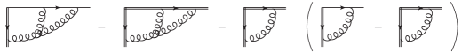
Figure 36: Representative diagrams illustrating double-hard-collinear contributions to the virtual two-loop amplitude along a single hard line.

Having at our disposal a full characterisation of double-virtual poles, we can now browse our list of local counterterms, given in Eq. (6.49) and Eq. (6.54), and extract the combinations we need: we are guided by the finiteness conditions

$$S_{n,0}^{(2)}\,+\,\int d\Phi_{1}(k)\,S_{n,\,1}^{(1)}(k)\,+\,\int d\Phi_{2}(k,k^{\prime})\,S_{n,\,2}^{(0)}(k,k^{\prime}) = {\rm finite}\,,$$

$$\int d\Phi_{1}\,J^{(2)}_{i,\,0}\,+\,\int d\Phi_{2}(k)\,J_{i,\,1}^{(1)}(k)\,+\,\int d\Phi_{3}(k,k^{\prime})\,J_{i,\,2}^{(0)}(k,k^{\prime}) = {\rm finite}\,,$$ (6.68)

(with a similar one for eikonal jets) which stem from the finiteness of Eq. (6.51) and Eq. (6.3). Quite naturally, one-loop functions with single radiation are assigned to the real-virtual counterterm $K_{n+1}^{\,(\mathbf{RV})}$, while tree-level functions with double radiation are assigned to the double-unresolved counterterm $K_{n+2}^{({\bf 2})}$.

Using these criteria on Eq. (6.4), one finds that the double-unresolved counterterm in the $({n+2})$-particle phase space, $K^{\,(\mathbf{2})}_{n+2}$, can be organised as

$$K_{n+2}^{\bf(2)}\,=\,K_{n+2}^{({\bf 2},\,{\rm 2s})}\,+\,\sum_{i=1}^{n}\bigg{[}K_{n+2,\,i}^{({\bf 2},\,\rm{2hc})}\,+\,\sum_{j=i+1}^{n}K_{n+2,\,ij}^{({\bf 2},\,\rm{2hc})}\,+\,K_{{n+2},\,i}^{({\bf 2},\,\rm{1hc,\,1s})}\bigg{]}\,,$$ (6.69)

where the notation mimicks Eq. (6.4). Explicit expressions for all the different contributions in Eq. (6.69) are too lengthy to list here, but they can be found in Ref. [295]. To illustrate their structure, we just report here the double-soft contribution, and the double-hard-collinear contribution arising from a single line. They are given by

$$K^{({\bf 2},\,{\rm 2s})}_{n+2} = {\cal H}^{(0)\,\dagger}_{n}\,S_{n,\,2}^{(0)}\,{\cal H}^{(0)}_{n}\,,$$

$$K^{({\bf 2},\,{\rm 2hc})}_{{n+2},\,i} = {\cal H}^{(0)\,\dagger}_{n}\Big{[}J^{(0)}_{i,\,2}-J_{i,\,{\mbox{\tiny{E}}},\,2}^{(0)}-J_{i,\,{\mbox{\tiny{E}}},\,1}^{(0)}\left(J^{(0)}_{i,\,1}-J_{i,\,{\mbox{\tiny{E}}},\,1}^{(0)}\right)\!\Big{]}S_{n,\,0}^{(0)}\,{\cal H}^{(0)}_{n}\,.$$ (6.70)

In the last line, we recognise the hard-collinear structure discussed above, and illustrated in Fig. 36, but this time applied to tree-level, double-radiative contributions.

In a similar vein, the real-virtual counterterm $K_{n+1}^{\,(\mathbf{RV})}$ has the structure

$$K_{n+1}^{\,(\mathbf{RV})}\,=\,K_{n+1}^{({\bf RV},\,{\rm s})}\,+\,\sum_{i=1}^{n}\bigg{[}K_{n+1,\,i}^{({\bf RV},\,\rm{2hc})}\,+\,\!\sum_{j=i+1}^{n}\!K_{n+1,\,ij}^{({\bf RV},\,\rm{2hc})}\,+\,K_{n+1,\,i}^{({\bf RV},\,\rm{1hc,\,1s})}\,+\,K_{n+1,\,i}^{({\bf RV},\,\rm{1hc})}\bigg{]}\,,$$ (6.71)

where, this time, the notation ‘2hc’ refers to a configuration with a hard collinear real gluon paired with the hard collinear poles arising from the loop integration. Once again we display only the soft component and the single-line hard-collinear component. They are

$$K^{({\bf RV},\,{\rm s})}_{n+1} = {\cal H}^{(0)\,\dagger}_{n}\,S_{n,\,1}^{(0)}\,{\cal H}^{(1)}_{n}\,+\,{\cal H}^{(1)\,\dagger}_{n}\,S_{n,\,1}^{(0)}\,{\cal H}^{(0)}_{n}\,+\,{\cal H}^{(0)\,\dagger}_{n}\,S_{n,\,1}^{(1)}\,{\cal H}^{(0)}_{n}\,,$$ (6.72)

$$K^{({\bf RV},\,{\rm 2hc})}_{{n+1},\,i} = {\cal H}^{(0)\,\dagger}_{n}\bigg{[}J^{(1)}_{i,\,1}-J_{i,{\mbox{\tiny{E}}},\,1}^{(1)}-\Big{(}J_{i,\,0}^{(1)}-J^{(1)}_{i,{\mbox{\tiny{E}}},\,0}\Big{)}J^{(0)}_{i,{\mbox{\tiny{E}}},\,1}-J_{i,{\mbox{\tiny{E}}},\,0}^{(1)}\Big{(}J^{(0)}_{i,\,1}-J^{(0)}_{i,{\mbox{\tiny{E}}},\,1}\Big{)}\bigg{]}S_{n,\,0}^{(0)}\,{\cal H}^{(0)}_{n}\,,$$

In the first line, we see that single soft radiation can be paired with the finite part of a one-loop contribution, while the last term involves the one-loop correction to the single-radiative soft function. In the second line, we again recognise a factorised structure similar to the one discussed in connection with Eq. (6.4): the first term in square brackets combines a collinear loop with a collinear radiation, including all soft regions; the second term subtracts the contribution where both the virtual and the real gluon are soft; the third term subtracts the region where the radiated gluon is soft, while the virtual one is hard and collinear, and finally the last term deals with the complementary region where the virtual gluon is soft, but the radiated one is hard and collinear.

These examples show how a factorisation approach provides a set of transparent expressions for candidate counterterms at NNLO, in a manner that can be directly generalised to higher orders. To complete the picture, we must however deal with the last remaining local counterterm, the $K^{\,(\mathbf{12})}_{n+2}$ function, which describes the overlap between single-unresolved and double-unresolved configurations in the $({n+2})$-particle phase space. It is natural to define the strongly-ordered counterterm as the collection of the single-unresolved limits of $K^{\,(\mathbf{2})}_{n+2}$: in this sense, one might do without an explicit definition of $K^{\,(\mathbf{12})}_{n+2}$ in terms of operator matrix elements, since the relevant soft and collinear limits can be easily computed once $K^{\,(\mathbf{2})}_{n+2}$ is known. We have seen however, in Section 6.3, that having a formal definition of the counterterm as a matrix element allows to prove the cancellation of divergences, to any order, in a straightforward way. It is therefore worthwhile to search for a general, formal definition of strongly-ordered local counterterms.

Here, we will simply illustrate how such a definition can be constructed in the case of tree-level emissions of soft gluons. It is not difficult to envisage the structure of the result in this case: if two soft gluons are emitted from a system of $n$ hard particles, and one of the two gluons is much softer than the other, the softer gluon, at leading power, will effectively arise from a configuration of ${n+1}$ hard particles, which will be represented by ${n+1}$ Wilson lines in the soft approximation. This soft factorisation will leave behind a hard matching function; however, since the exact result for the double soft emission when both soft gluons scale in the same way is known, and is expressed as a matrix element of $n$ Wilson lines, it is natural to guess that the hard matching function for the softest emission will be given by the matrix element for the emission of the harder gluon from the original $n$ Wilson lines. This translates into the following tree-level ansatz for the strongly-ordered soft function for double gluon emission from $n$ hard particles:

$$\Big{[}{\cal S}^{(0)}_{n;\,1,\,1}\Big{]}^{a_{i}a_{j}}_{\{d_{m}e_{m}\}}\big{(}k_{i},k_{j};\{\beta_{m}\}\big{)} \equiv \left\langle\smash{k_{j},a_{j}}{\vphantom{1}}\right|\,\Big{[}\Phi_{\beta_{i}}(0,\infty)\Big{]}^{a_{i}b}\prod_{m=1}^{n}\Big{[}\Phi_{\beta_{m}}(0,\infty)\Big{]}_{d_{m}}^{\,\,\,\,c_{m}}\left|\smash{0}{\vphantom{1}}\right\rangle$$

$$\hskip 28.45274pt\times\,\left\langle\smash{k_{i},b}{\vphantom{1}}\right|\,\prod_{m=1}^{n}\Big{[}\Phi_{\beta_{m}}(0,\infty)\Big{]}_{c_{m}e_{m}}\left|\smash{0}{\vphantom{1}}\right\rangle\Big{|}_{\rm tree}$$

$$= \left[{\cal S}^{(0)}_{n+1,1}\right]^{a_{j},\,a_{i}b}_{\{d_{m}c_{m}\}}\big{(}k_{j};\beta_{i},\{\beta_{m}\}\big{)}\,\left[{\cal S}^{(0)}_{n,1}\right]_{b,\,\{c_{m}e_{m}\}}\!\big{(}k_{i};\{\beta_{m}\}\big{)}\,,$$

where we wrote explicitly all colour indices, including the colour indices of the two ordered soft gluons in the final state bra vectors. The physical interpretation of Eq. (6.4) is the following: in the limit $k_{j}\ll k_{i}$, the hierarchy between the two soft gluon momenta states that $k_{i}$ is soft with respect to the $n$ Born-level hard partons, but it is hard if compared with the softest radiation $k_{j}$. This means that gluon $j$ cannot resolve the different energy scales of the other ${n+1}$ partons, since their momenta are all much greater than $k_{j}$: thus, from the point of view of gluon $j$, gluon $i$ can be treated as another classical source of soft radiation, represented by its own Wilson line. According to this picture, in the first line of Eq. (6.4) the emission of gluon $j$ is modelled at leading power by a Wilson-line correlator, where one of the $n+1$ lines carries the quantum numbers of gluon $i$, including colour, and is directed along momentum $k_{i}$. Next, in the second line of Eq. (6.4), the emission of gluon $i$ is described by a single-radiative soft function, involving the $n$ Born-level hard particles. This configuration is schematically represented in Fig. 37, in the simplest case with $n=2$. The blue curly line in the first bracket corresponds to gluon $i$, which behaves as a soft gluon when emitted from the Born particles, but acts as a hard particle, represented by the blue Wilson line in the second bracket, when gluon $j$ is emitted. Note that the colour structure of Eq. (6.4) is crucial: the first eikonal form factor acts as a colour operator on the second form factor, with the adjoint index $b$ of the Wilson line associated with gluon $i$ contracting with the index of the gluon state in the second line.

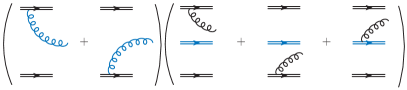
Figure 37: A simple example of the re-factorisation of an eikonal form factor in a strongly-ordered limit, with $n=2$ Born-level particles.

It is easy to verify that the definition in Eq.(6.4) returns precisely

$$\Big{[}{\cal S}^{(0)}_{n;\,1,\,1}\Big{]}^{a_{i}a_{j}}\big{(}k_{i},k_{j};\{\beta_{m}\}\big{)}=\epsilon^{*\,\mu_{i}}(k_{i})\;\epsilon^{*\,\mu_{j}}(k_{j})\,\left[J^{(0),\,\rm s.o.}\right]_{\mu_{i}\mu_{j}}^{a_{i}a_{j}}\big{(}k_{i},k_{j};\{\beta_{m}\}\big{)}\,,$$ (6.74)

where the strongly-ordered current on the r.h.s. was introduced in Eq. (6.1). The strongly-ordered double-soft counterterm $K^{\,(\mathbf{12}),\,\rm s}_{n+2}$ is then obtained by squaring Eq. (6.4), in analogy to Eq. (6.49). Clearly, the re-factorisation in Eq. (6.4) is only the simplest example of an infinite tower of similar expressions, when multiple soft gluons are emitted with different hierarchical patterns. For example, it can be verified that formulas with the same structure as Eq. (6.4) correctly generate the strongly ordered limits for triple and quadruple tree-level soft emissions, which can be checked with the complete limits computed in Ref. [539]. Furthermore, Eq. (6.4) naturally lends itself to an all-order interpretation, where loop corrections can be distributed between the two radiative soft functions on the r.h.s. Strongly-ordered collinear limits are somewhat more intricate, due to the need to perform spin sums, and to the fact that the jet functions that we are employing contain collinear-finite contributions: a similar tree-level pattern, however, emerges. We believe that this kind of re-factorisation can shed light on the all-order structure of multiple soft and collinear emissions, with significant applications for subtraction at high orders, which are under study.

7 Perspectives

Our journey through the infrared comes to an end. The journey has been long – it had to be, given the long history of the subject. Yet we regret that, limited by space and by the knowledge span of the authors, it has barely touched many interesting issues, and it has mentioned only in passing several important lines of enquiry.

The first part of the journey has been an overview of history. We started in Section 1.1 by presenting the Bloch-Nordsieck theorem, which displays for the first time the mechanism for the cancellation of infrared divergences, and gives the first example of factorisation and exponentiation of real and virtual radiative corrections, in the context of QED. The physical origin of the problem – the mistake that leads to the failure of the standard perturbative approach in the presence of massless particles – was already correctly diagnosed at that time, as was the path to a general solution.

As we have seen, however, the infrared problem has been solved many times, from different conceptual angles, with increasing degrees of sophistication, and uncovering deeper layers of structure. In this respect, the history of the infrared problem parallels the history of the ultraviolet one, which also fruitfully evolved through several levels of interpretation and many technical developments.

The Bloch-Nordsieck approach reaches its maximal range with the KLN theorem, discussed in Section 1.2, which proves that the mechanism of real-virtual cancellation is completely general, and applies to any quantum-mechanical theory containing states that are degenerate in energy. While this provides a solid foundation for all subsequent developments, it cannot be considered completely satisfactory, since it applies only at the level of sufficiently inclusive cross sections, bypassing the $S$-matrix, which historically has been – and to this day remains – a crucial quantity for most developments in quantum field theory. The first answer to this omission is the construction of a Hilbert space of coherent states, which leads to the formal definition of an infrared-finite $S$-matrix both in abelian and in non-abelian theories, as reviewed in Section 1.3.

The advent of non-abelian gauge theories posed novel problems at two different levels, and in turn led to a whole series of new developments that are far from exhausted. On the one hand, there are conceptual problems, arising directly at the non-perturbative level, at least in the case of confining gauge theories like QCD. Indeed, QCD has an added layer of mystery to it: quarks and gluons – the perturbative degrees of freedom – cannot be observed as asymptotic states, unlike their electroweak counterparts; they are confined. This drastic discrepancy between perturbative and non-perturbative asymptotic states leads to great difficulties both for a KLN approach – since the sum over degenerate initial states containing short-distance degrees of freedom does not correspond directly to any physical observable – and for the coherent state construction, which so far has been achieved only at the level of perturbation theory. On the other hand, there are technical and practical problems, increasingly related to the spectacular progress of accelerator experiments, now reaching extraordinary levels of precision even for intricate collider observables. A key technical problem is the unavoidable presence of collinear divergences, directly related to the masslessness of gauge bosons; a general practical problem is the development of perturbative techniques to high enough orders, so as to match the precision reached by collider experiments.

Our current best answer to both the conceptual and the practical challenges posed by non-abelian gauge theories is the factorisation program, both at the level of inclusive cross sections and at the level of scattering amplitudes. Thus, most of our review has been devoted to the development of perturbative tools for factorisation, and to their concrete application to fixed-angle scattering amplitudes and to real radiation of soft and collinear particles.

The physical ideas underpinning factorisation are as powerful as they are simple and intuitive. Processes taking place at very different length (or energy) scales must be decoupled to a large extent: thus for example we don’t expect the size of the laboratory to play a role in elementary particle collisions, nor do we expect subatomic events to influence how rivers flow. Quantum mechanics challenges this simple picture, forcing us – in principle – to take into account all physical scales simultaneously. Recovering the factorised, semiclassical picture with conventional perturbative tools is possible, but hard, since the contributions of different physical scales are scattered across a plethora of Feynman diagrams, additively building up the observable at each perturbative order.

In the infrared domain, we have sketched the rather winding path that finally organises perturbative contributions to quantum amplitudes into a product of factors, each responsible for phenomena occurring at a specific physical scale. After introducing some tools by means of one-loop examples in Section 2, we proceeded in Section 3 by outlining an all-order diagrammatic analysis. Remarkably, the infinite taxonomy of Feynman diagrams can be tamed, and singular contributions located and organised. Once the physical scales relevant for a particular observable have been identified, one can proceed with the tools of effective field theories, which naturally lead to factorised expressions for the observable. On the other hand, the same diagrammatic analysis that succeeded in locating singular contributions motivates the construction of universal functions responsible for infrared enhancements, taking into account the constraints of gauge invariance, as discussed in Section 3.3.

Once factorisation is achieved, be it in the infrared or in the ultraviolet, it provides a precise mathematical expression for the idea of universality: that only limited information can be transferred between physical scales separated by wide gaps. In the ultraviolet, in the case of renormalizable theories, one finds that very high-energy degrees of freedom can influence low-energy scattering only by tuning coupling constants; in the infrared, one similarly finds that long-distance effects can be captured by a small set of functions, introduced here in Section 4.1, which can be defined independently of the particular scattering process under consideration.

Even more importantly, factorisation inevitably leads to the existence of evolution equations. Physical observables cannot depend on the artificial parameters that theorists must introduce to define the relevant scale domains, whether they take the form of factorisation scales, separating ultraviolet from infrared phenomena, or factorisation vectors, separating collinear from wide-angle dynamics. This independence translates into evolution equations, discussed here in Section 4.2. Solving these equations, in turn, leads to a resummation of perturbation theory in the relevant kinematic domain. Universal quantities are then expressed in terms of anomalous dimensions, which naturally become the cornerstone of perturbative calculations. Already at the level of massless form factors, a prominent role is played in particular by the light-like cusp anomalous dimension $\gamma_{K}(\alpha_{s})$, which governs the soft limit of virtual exchanges.

Moving on from form factors to multi-particle fixed-angle scattering amplitudes, discussed in Section 5, one encounters a significant step, both conceptual and technical: soft anomalous dimensions become colour matrices, and their high-order colour structure, which is highly non-trivial, becomes an important focus of investigation. In Section 5.2 and in Section 5.3 we studied the all-order structure of infrared anomalous dimensions matrices, and we introduced different methods for computing them, uncovering in the process remarkable links to the Regge limit and to conformal field theories on the celestial sphere.

Factorisation and universality apply to real radiation too, as must be the case in order for the KLN theorem to work with the expected generality. The factorisation of scattering amplitudes in soft and collinear limits, which is by itself a vast field of research, has been briefly reviewed here in Section 6.1. Even when the soft and collinear factorisation kernels are known to a given order, efficiently organising the KLN cancellation at high orders remains a challenge. In the remaining part of Section 6, we have discussed modern approaches to tackle this subtraction problem. Our aim there was not to review existing methods, which were recently discussed in Ref. [82]; rather, we tried to display the link between the factorisation of virtual corrections and that of real emission, presenting a general strategy to define soft and collinear local counterterms, which are universal, and constructed to manifestly cancel virtual poles to any order. We also pointed out the significant technical difficulties that must still be tackled, on the way to an efficient implementation, even when the form of the local counterterms is known.

One may wonder at this point what the future holds, as the second century of infrared studies lies just below the future horizon. There are certainly many open lines of developments, as well as a few dreams.

A first obvious direction of further studies is dictated by the quest for precision which characterises current high-energy research. Clearly, fully general and efficient subtraction algorithms, working beyond NLO, will be needed in the upcoming phases of the LHC program, as well as for other present and future colliders. Given the pace of present developments, and the resources that are devoted to this effort by many groups, it is to be fully expected that more than one such algorithm will be made available at NNLO within the next few years. NNLO algorithms will then have to be fully integrated with event generators and parton showers at that accuracy, which in itself will be a non-trivial task. One may be somewhat bolder: since most real-radiation kernels required for N³LO calculations are already known, as is the full set of three-loop infrared anomalous dimensions, it is to be expected that a similar effort towards generality and efficiency will be applied at N³LO. Along the way, many technical question will hopefully find answers: for example, concerning the all-order structure of soft and collinear local counterterms, including those for strongly-ordered configurations, and concerning the optimisation of the phase-space mappings required to match radiative and Born-level momentum configurations.

On the side of virtual corrections, the goal of having a full set of soft and collinear anomalous dimensions for massless scattering at the four-loop order appears reachable within a similar time scale. Achieving this result would have practical implications, allowing for soft gluon resummations (in the threshold, $p_{T}$ and high-energy domains) with impressive logarithmic accuracies, and permitting highly non-trivial studies of the convergence properties of resummed perturbation theory for complex collider processes. Furthermore, there are also interesting theoretical issues that start being accessible at such high orders. An important example is the role played by higher-order Casimir invariants, which appear for the first time at four loops, and subsequently build up their own perturbative expansion. The role of these complex colour structures in the factorisation program, and more generally in the dynamics of high-energy scattering, is largely unexplored to this day.

Performing such high-order calculations for infrared divergences may require new technical developments, on a par with those that have facilitated the calculation of multi-loop Feynman integrals in recent years. Empirically, current techniques for the evaluation of Wilson-line correlators, which are based on Feynman diagrams, seem to suffer from the same drawbacks that have been many times lamented for the case scattering amplitudes. Both colour and kinematic dependences of Wilson-line correlators display large-scale complexity in the intermediate stages of calculations, while the final results are remarkably simple and elegant. This is certainly the case for the massless soft anomalous dimension matrix at three loops, and for the massive correction at two loops. One feels that the simplicity of the final result is at least partly unexplained, and obscured in the various stages of the calculation by many unphysical dependences, such as the gauge redundance and the reliance on different regulators to tame the intricate singularity structure.

In this regard, Wilson line correlators that are relevant for the infrared limit differ in two important ways from ordinary amplitudes. First, their integrands involve denominators linear in momenta: this is an important difference in view of applying standard methods for the calculation of multi-loop Feynman integrals, such as integration by parts and differential equations [627]. While existing methods and codes can be generalised to include linear denominators, it is clear that they are not optimised for this purpose. A second aspect is the strong dependence of eikonal integrals on auxiliary soft and collinear regulators, such as the exponential regulator introduced in Eq. (5.70): while the final results for anomalous dimensions are independent of the chosen regulators, intermediate steps in the calculation are heavily affected. Regularisation procedures that work well for the purposes of analytic calculations performed with pencil and paper at low orders are not necessarily optimal for automatic evaluation of high-order corrections using existing algorithms. Both these problems can probably be attacked by generalising to Wilson-line correlators some of the techniques that have been developed in recent years for the calculation of scattering amplitudes and form factors. In particular, generalised unitarity surely applies in the presence of Wilson lines [628, 629], albeit in a somewhat unconventional manner; similarly, general tools such as intersection theory [630] are likely to be applicable also in this context; finally, a bootstrap approach, based on the identification of the function space comprising the correlators, followed by the implementation of symmetry, kinematic and dynamical constraints, has already been shown to be very powerful.

Moving on from technical aspects to more general and long-term prospects, we believe that it is fair to say that infrared factorisation for real soft and collinear radiation is less developed than is the case for virtual corrections to fixed-angle scattering amplitudes. While general theorems exist, the detailed structure of soft and collinear kernels at high orders becomes increasingly complex, and only limited handles are available to organise and disentangle this complexity. Clearly, to some extent this is an inevitable consequence of the fact that real radiation kernels are differential quantities, allowing for an intricate dependence on the momenta and quantum numbers of soft and collinear particles. On the other hand, the comparative simplicity of the singularity structure of virtual corrections should provide organising principles for real radiation as well, given the general theorems on the cancellation of divergences. At a minimum, as an effect of the KLN theorem, virtual corrections must provide sum rules for real radiation kernels, whose phase-space integrals must cancel virtual poles: this viewpoint is at the basis of the organisation of subtraction counterterms discussed in Section 6.3. One may, however, hope for a deeper understanding: for example, the exponentiation of virtual poles, which implies subtle correlations between results at different perturbative orders, should be reflected in a similar organisation for real radiation corrections. An interesting first step in this direction was taken in Ref. [539], where a form of exponentiation of soft real radiation in terms of a generating functional was suggested.

More generally, an important and largely unexplored issue is the connection between fixed-angle scattering and the limits in which strong hierarchies develop between Mandelstam invariants, ultimately leading to singular behaviours. Soft and collinear configurations belong to this category, but also Regge and multi-Regge limits. Large logarithms that appear in these limits, endangering the reliability of perturbation theory, are tightly connected with infrared enhancements: while this connection has been understood and exploited for a long time, it is likely that much more structure remains to be uncovered.

Finally, we turn to ultimate targets, beyond the range of predictable developments and into the sphere of speculations and perhaps dreams. While almost everything we have written has been strictly perturbative, it must be noted that in the infrared domain one can typically derive resummed results which contain information to all orders in perturbation theory. It is inevitable then to muse on the possibility that, through an infrared portal, one might access truly non-perturbative information. In a limited sense, this is certainly true and well known: indeed, as briefly discussed in the Introduction, summations of perturbation theory inevitably display the divergence of the perturbative expansion, and a detailed analysis of the divergent behaviour yields parametric information on non-perturbative corrections (see, for example, [631, 632, 633]. On the other hand, it is perhaps reasonable to hope for much more detailed information. First of all, we note that infrared factorisation localises long-distance information in a set of universal functions which are given by matrix elements of local and non-local operators, and these matrix elements are in principle well defined in the full gauge theory, beyond the perturbative domain. These functions can then be studied with non-perturbative methods, at times with direct phenomenological applications, as was done for example in Ref. [634]. Furthermore, even when resumming infrared poles, which has been the focus of our review, one can uncover relations between matrix elements and anomalous dimensions which are expected to be valid beyond perturbation theory, as was the case in Ref. [70], with the refinements later introduced in Ref. [572]. For special, highly symmetric gauge theories these relations can sometimes be tested non-perturbatively, as was done for example in Refs. [367, 380]. Note that the relations we are discussing connect finite quantities, a prime example being Eq. (4.39).

For confining gauge theories, non-perturbative effects must ultimately entangle colour and kinematic degrees of freedom at large distances, forcing the flow of soft radiation towards the formation of colour-singlet states. The first occurence of such a colour-kinematic entanglement to all orders in perturbation theory takes place at the level of soft anomalous dimensions, as exemplified by Eq. (5.35) and Eq. (5.2). Clearly, one sees no trace of confinement at this level (indeed, the expressions we are discussing are common to confining gauge theories like pure Yang-Mills, and to conformal gauge theories like ${\cal N}=4$ super-Yang-Mills theory). One can however hope that the language of soft anomalous dimensions could be used to access and study non-perturbative aspects as well. The novel viewpoint introduced in Refs. [147] is perhaps the most promising in this regard, provided it can be consistently extended and understood to include quantum corrections and collinear dynamics. As suggested by the discussion in Section 5.2.2, based on Ref. [164], this may indeed be possible. In the dipole approximation, the picture painted by the celestial approach is that of a Coulomb gas of two-dimensional coloured particles with pairwise interactions on the celestial sphere; furthermore, we already know that this picture will receive corrections involving multi-particle interactions on the sphere, which could lead to clustering in appropriate circumstances. Most importantly, the two-dimensional theory on the sphere, once properly identified, could be studied with non-perturbative tools: if it turned out to be locally conformal invariant, which seems likely, it could well be solvable. This would provide a completely new and remarkable window on the long-distance behaviour of non-abelian gauge theories.

References

- [1] M. E. Peskin and D. V. Schroeder, An Introduction to Quantum Field Theory. Taylor & Francis Group LLC, USA, 1995.
- [2] G. F. Sterman, An Introduction to Quantum Field Theory. Cambridge University Press, Cambridge, UK, 1993.
- [3] G. Farmelo, The Strangest Man. Faber and Faber, London, UK, 2009. See in particular the conversation reported in Chapter XX.
- [4] G. P. Lepage, “What is Renormalization?,” in Theoretical Advanced Study Institute in Elementary Particle Physics, pp. 483–508. 6, 1989. hep-ph/0506330.
- [5] M. Neubert, “Renormalization Theory and Effective Field Theories,” Les Houches Lect. Notes 108 (2020) 1901.06573.
- [6] F. J. Dyson, “Divergence of perturbation theory in quantum electrodynamics,” Phys. Rev. 85 (1952) 631–632.
- [7] J. C. Le Guillou and J. Zinn-Justin, eds., Large order behavior of perturbation theory. North Holland, 1990.
- [8] B. E. Lautrup, “On High Order Estimates in QED,” Phys. Lett. B 69 (1977) 109–111.
- [9] C. M. Bender and T. T. Wu, “Anharmonic oscillator. II: A Study of perturbation theory in large order,” Phys. Rev. D 7 (1973) 1620–1636.
- [10] C. M. Bender, “Perturbation Theory in Large Order,” Adv. Math. 30 (1978) 250–267.
- [11] M. Beneke, “Renormalons,” Phys. Rept. 317 (1999) 1–142, hep-ph/9807443.
- [12] M. Mariño, “Lectures on non-perturbative effects in large gauge theories, matrix models and strings,” Fortsch. Phys. 62 (2014) 455–540, 1206.6272.
- [13] I. Aniceto, G. Basar, and R. Schiappa, “A Primer on Resurgent Transseries and Their Asymptotics,” Phys. Rept. 809 (2019) 1–135, 1802.10441.
- [14] O. Costin and G. V. Dunne, “Physical Resurgent Extrapolation,” Phys. Lett. B 808 (2020) 135627, 2003.07451.
- [15] N. Mott, “On the influence of radiative forces on the scattering of electrons,” Proc. Camb. Phil. Soc. 27 (1931) 255.
- [16] A. Sommerfeld, “Über die beugung und bremsung der elektronen,” Annalen der Physik 403 (1931), no. 3, 257.
- [17] H. Bethe and W. Heitler, “On the Stopping of fast particles and on the creation of positive electrons,” Proc. Roy. Soc. Lond. A 146 (1934) 83–112.
- [18] F. Bloch and A. Nordsieck, “Note on the Radiation Field of the electron,” Phys. Rev. 52 (1937) 54–59.
- [19] J. Jauch and F. Rohrlich, “The infrared divergence,” Helvetica Physica Acta 27 (1954) 613.
- [20] D. R. Yennie, S. C. Frautschi, and H. Suura, “The infrared divergence phenomena and high-energy processes,” Annals Phys. 13 (1961) 379–452.
- [21] G. Grammer, Jr. and D. R. Yennie, “Improved treatment for the infrared divergence problem in quantum electrodynamics,” Phys. Rev. D8 (1973) 4332–4344.
- [22] T. Kinoshita, “Mass singularities of Feynman amplitudes,” J. Math. Phys. 3 (1962) 650–677.
- [23] T. D. Lee and M. Nauenberg, “Degenerate Systems and Mass Singularities,” Phys. Rev. 133 (1964) B1549–B1562. [,25(1964)].
- [24] J. Dollard, “Asymptotic convergence and the coulomb interaction,” J. Math. Phys. 5 (1964) 729.
- [25] V. Chung, “Infrared Divergence in Quantum Electrodynamics,” Phys. Rev. 140B (1965) 1110.
- [26] E. S. Fradkin, “Method of Green’s functions in quantum field theory and quantum statistics,” Trud. Fiz. Inst. Akad. Nauk SSSR (Fiz. Inst. Lebedev) 29 (1965) 7–138.
- [27] T. Kibble, “Coherent soft-photon states and infrared divergences. iii. asymptotic states and reduction formulas,” Phys. Rev. 174 (1968) 1882.
- [28] T. Kibble, “Coherent soft-photon states and infrared divergences. ii. mass-shell singularities of green’s functions,” Phys. Rev. 173 (1968) 1527.
- [29] T. Kibble, “Coherent soft-photon states and infrared divergences. iv. the scattering operator,” Phys. Rev. 175 (1968) 1624.
- [30] P. Kulish and L. Faddeev, “Asymptotic conditions and infrared divergences in quantum electrodynamics,” Theor. Math. Phys. 4 (1970) 745.
- [31] E. C. Poggio and H. R. Quinn, “The Infrared Behavior of Zero-Mass Green’s Functions and the Absence of Quark Confinement in Perturbation Theory,” Phys. Rev. D 14 (1976) 578.
- [32] G. F. Sterman, “Kinoshita’s Theorem in Yang-Mills Theories,” Phys. Rev. D 14 (1976) 2123–2125.
- [33] T. Kinoshita and A. Ukawa, “Structure of Leading Infrared Divergences in Nonabelian Gauge Theories,” Phys. Rev. D 16 (1977) 332.
- [34] R. Doria, J. Frenkel, and J. Taylor, “Counter Example to Nonabelian Bloch-Nordsieck Theorem,” Nucl. Phys. B 168 (1980) 93–110.
- [35] C. Di’Lieto, S. Gendron, I. Halliday, and C. T. Sachrajda, “A Counter Example to the Bloch-Nordsieck Theorem in Nonabelian Gauge Theories,” Nucl. Phys. B 183 (1981) 223–250.
- [36] A. Andrasi, M. Day, R. Doria, J. Frenkel, and J. Taylor, “Soft Divergences in Perturbative QCD,” Nucl. Phys. B 182 (1981) 104–124.
- [37] C. Carneiro, M. Day, J. Frenkel, J. Taylor, and M. Thomaz, “Leading non-cancelling infrared divergences in perturbative QCD,” Nucl. Phys. B 183 (1981) 445–470.
- [38] J. Frenkel, J. Gatheral, and J. Taylor, “Is quark-antiquark annihilation infrared-safe at high energy?,” Nucl. Phys. B 233 (1984) 307–335.
- [39] M. Ciafaloni, P. Ciafaloni, and D. Comelli, “Bloch-Nordsieck violation in spontaneously broken Abelian theories,” Phys. Rev. Lett. 87 (2001) 211802, hep-ph/0103315.
- [40] S. Catani, “Violation of the Bloch-nordsieck Mechanism in General Nonabelian Theories and SUSY QCD,” Z. Phys. C 37 (1988) 357.
- [41] F. Caola, K. Melnikov, D. Napoletano, and L. Tancredi, “Noncancellation of infrared singularities in collisions of massive quarks,” Phys. Rev. D 103 (2021), no. 5, 054013, 2011.04701.
- [42] S. B. Libby and G. F. Sterman, “Cancellation of Infrared Divergences in Massive Quark Potential Scattering,” Phys. Rev. D 19 (1979) 2468.
- [43] R. Akhoury, “Mass Divergences of Wide Angle Scattering Amplitudes,” Phys. Rev. D 19 (1979) 1250.
- [44] V. Ganapathi and G. F. Sterman, “Infrared Divergences in Quark Potential Scattering,” Phys. Rev. D 23 (1981) 2408.
- [45] J. C. Collins and G. F. Sterman, “Soft Partons in QCD,” Nucl. Phys. B 185 (1981) 172–188.
- [46] M. Greco, F. Palumbo, G. Pancheri-Srivastava, and Y. Srivastava, “Coherent State Approach to the Infrared Behavior of Nonabelian Gauge Theories,” Phys. Lett. B 77 (1978) 282.
- [47] G. Curci and M. Greco, “Mass Singularities and Coherent States in Gauge Theories,” Phys. Lett. B 79 (1978) 406.
- [48] D. Butler and C. Nelson, “Nonabelian Structure of Yang-Mills Theory and Infrared Finite Asymptotic States,” Phys. Rev. D 18 (1978) 1196.
- [49] G. Curci, M. Greco, and Y. Srivastava, “QCD Jets From Coherent States,” Nucl. Phys. B 159 (1979) 451.
- [50] C. Nelson, “Avoidance of Counter Example to Nonabelian Bloch-Nordsieck Conjecture by Using Coherent State Approach,” Nucl. Phys. B 186 (1981) 187.
- [51] C. Nelson, “Origin of Cancellation of Infrared Divergences in Coherent State Approach: Forward Process + Gluon,” Nucl. Phys. B 181 (1981) 141.
- [52] T. Muta and C. A. Nelson, “Role of Quark - Gluon Degenerate States in Perturbative QCD,” Phys. Rev. D 25 (1982) 2222.
- [53] M. Ciafaloni, “The QCD Coherent State From Asymptotic Dynamics,” Phys. Lett. B 150 (1985) 379.
- [54] S. Catani, M. Ciafaloni, and G. Marchesini, “Asymptotic Coherent States and Color Screening,” Phys. Lett. B 168 (1986) 284.
- [55] S. Catani, M. Ciafaloni, and G. Marchesini, “Non-cancelling infrared divergences in QCD coherent state,” Nucl. Phys. B 264 (1986) 588.
- [56] S. Catani and M. Ciafaloni, “Gauge covariance of QCD coherent states,” Nucl. Phys. B 289 (1987) 535.
- [57] V. Del Duca, L. Magnea, and G. F. Sterman, “Collinear Infrared Factorization and Asymptotic Evolution,” Nucl. Phys. B 324 (1989) 391.
- [58] M. Ciafaloni, “Infrared singularities and coherent states in gauge theories,” Adv. Ser. Direct. High Energy Phys. 5 (1989) 491–572.
- [59] G. Giavarini and G. Marchesini, “IR Finite S Matrix in the QCD Coherent State Basis,” Nucl. Phys. B 296 (1988) 546.
- [60] J. C. Collins, D. E. Soper, and G. F. Sterman, “Factorization of Hard Processes in QCD,” Adv. Ser. Direct. High Energy Phys. 5 (1988) 1–91, hep-ph/0409313.
- [61] G. F. Sterman, “Partons, factorization and resummation, TASI 95,” in Theoretical Advanced Study Institute in Elementary Particle Physics (TASI 95): QCD and Beyond, pp. 327–408. 6, 1995. hep-ph/9606312.
- [62] V. V. Sudakov, “Vertex parts at very high-energies in quantum electrodynamics,” Sov. Phys. JETP 3 (1956) 65–71. [Zh. Eksp. Teor. Fiz. 30, 87 (1956)].
- [63] A. H. Mueller, “On the Asymptotic Behavior of the Sudakov Form-factor,” Phys. Rev. D20 (1979) 2037.
- [64] J. C. Collins, “Algorithm to Compute Corrections to the Sudakov Form-factor,” Phys. Rev. D22 (1980) 1478.
- [65] A. Sen, “Asymptotic Behavior of the Sudakov Form-Factor in QCD,” Phys. Rev. D24 (1981) 3281.
- [66] A. Sen, “Asymptotic Behavior of the Wide Angle On-Shell Quark Scattering Amplitudes in Nonabelian Gauge Theories,” Phys. Rev. D 28 (1983) 860.
- [67] J. Collins, Foundations of perturbative QCD, vol. 32 of Cambridge Monographs on Particle Physics, Nuclear Physics and Cosmology. Cambridge University Press, 2013.
- [68] L. Magnea and G. F. Sterman, “Analytic continuation of the Sudakov form-factor in QCD,” Phys. Rev. D42 (1990) 4222–4227.
- [69] L. Magnea, “Analytic resummation for the quark form-factor in QCD,” Nucl. Phys. B 593 (2001) 269–288, hep-ph/0006255.
- [70] L. J. Dixon, L. Magnea, and G. F. Sterman, “Universal structure of subleading infrared poles in gauge theory amplitudes,” JHEP 08 (2008) 022, 0805.3515.
- [71] S. M. Aybat, L. J. Dixon, and G. F. Sterman, “The Two-loop soft anomalous dimension matrix and resummation at next-to-next-to leading pole,” Phys. Rev. D74 (2006) 074004, hep-ph/0607309.
- [72] S. M. Aybat, L. J. Dixon, and G. F. Sterman, “The Two-loop anomalous dimension matrix for soft gluon exchange,” Phys. Rev. Lett. 97 (2006) 072001, hep-ph/0606254.
- [73] T. Becher and M. Neubert, “Infrared singularities of scattering amplitudes in perturbative QCD,” Phys. Rev. Lett. 102 (2009) 162001, 0901.0722. [Erratum: Phys. Rev. Lett.111,no.19,199905(2013)].
- [74] E. Gardi and L. Magnea, “Factorization constraints for soft anomalous dimensions in QCD scattering amplitudes,” JHEP 03 (2009) 079, 0901.1091.
- [75] T. Becher and M. Neubert, “On the Structure of Infrared Singularities of Gauge-Theory Amplitudes,” JHEP 06 (2009) 081, 0903.1126. [Erratum: JHEP11,024(2013)].
- [76] E. Gardi and L. Magnea, “Infrared singularities in QCD amplitudes,” Frascati Phys. Ser. 50 (2010) 137–157, 0908.3273.
- [77] O. Almelid, C. Duhr, and E. Gardi, “Three-loop corrections to the soft anomalous dimension in multileg scattering,” Phys. Rev. Lett. 117 (2016), no. 17, 172002, 1507.00047.
- [78] C. Anastasiou, Z. Bern, L. J. Dixon, and D. A. Kosower, “Planar amplitudes in maximally supersymmetric Yang-Mills theory,” Phys. Rev. Lett. 91 (2003) 251602, hep-th/0309040.
- [79] Z. Bern, L. J. Dixon, and V. A. Smirnov, “Iteration of planar amplitudes in maximally supersymmetric Yang-Mills theory at three loops and beyond,” Phys. Rev. D 72 (2005) 085001, hep-th/0505205.
- [80] S. Frixione, Z. Kunszt, and A. Signer, “Three jet cross-sections to next-to-leading order,” Nucl. Phys. B 467 (1996) 399–442, hep-ph/9512328.
- [81] S. Catani and M. Seymour, “A general algorithm for calculating jet cross-sections in nlo qcd,” Nucl. Phys. B 485 (1997) 291–419, hep-ph/9605323. [Erratum: Nucl.Phys.B 510, 503–504 (1998)].
- [82] W. J. Torres Bobadilla et al., “May the four be with you: Novel IR-subtraction methods to tackle NNLO calculations,” Eur. Phys. J. C 81 (2021), no. 3, 250, 2012.02567.
- [83] E. Laenen, “Resummation for observables at TeV colliders,” Pramana 63 (2004) 1225–1249.
- [84] G. Luisoni and S. Marzani, “QCD resummation for hadronic final states,” J. Phys. G 42 (2015), no. 10, 103101, 1505.04084.
- [85] A. Banfi, G. P. Salam, and G. Zanderighi, “Principles of general final-state resummation and automated implementation,” JHEP 03 (2005) 073, hep-ph/0407286.
- [86] A. Banfi, H. McAslan, P. F. Monni, and G. Zanderighi, “A general method for the resummation of event-shape distributions in annihilation,” JHEP 05 (2015) 102, 1412.2126.
- [87] C. W. Bauer, S. Fleming, and M. E. Luke, “Summing Sudakov logarithms in B — X(s gamma) in effective field theory,” Phys. Rev. D 63 (2000) 014006, hep-ph/0005275.
- [88] C. W. Bauer, S. Fleming, D. Pirjol, and I. W. Stewart, “An Effective field theory for collinear and soft gluons: Heavy to light decays,” Phys. Rev. D 63 (2001) 114020, hep-ph/0011336.
- [89] C. W. Bauer and I. W. Stewart, “Invariant operators in collinear effective theory,” Phys. Lett. B 516 (2001) 134–142, hep-ph/0107001.
- [90] C. W. Bauer, D. Pirjol, and I. W. Stewart, “Soft collinear factorization in effective field theory,” Phys. Rev. D 65 (2002) 054022, hep-ph/0109045.
- [91] M. Beneke, A. P. Chapovsky, M. Diehl, and T. Feldmann, “Soft collinear effective theory and heavy to light currents beyond leading power,” Nucl. Phys. B 643 (2002) 431–476, hep-ph/0206152.
- [92] M. Beneke and T. Feldmann, “Multipole expanded soft collinear effective theory with nonAbelian gauge symmetry,” Phys. Lett. B 553 (2003) 267–276, hep-ph/0211358.
- [93] R. J. Hill and M. Neubert, “Spectator interactions in soft collinear effective theory,” Nucl. Phys. B 657 (2003) 229–256, hep-ph/0211018.
- [94] G. Parisi, “On Infrared Divergences,” Nucl. Phys. B 150 (1979) 163–172.
- [95] I. Feige and M. D. Schwartz, “Hard-Soft-Collinear Factorization to All Orders,” Phys. Rev. D90 (2014), no. 10, 105020, 1403.6472.
- [96] T. Becher, A. Broggio, and A. Ferroglia, “Introduction to Soft-Collinear Effective Theory,” Lect. Notes Phys. 896 (2015) pp.1–206, 1410.1892.
- [97] C. Lee and G. F. Sterman, “Momentum Flow Correlations from Event Shapes: Factorized Soft Gluons and Soft-Collinear Effective Theory,” Phys. Rev. D 75 (2007) 014022, hep-ph/0611061.
- [98] M. Bonvini, S. Forte, M. Ghezzi, and G. Ridolfi, “Threshold Resummation in SCET vs. Perturbative QCD: An Analytic Comparison,” Nucl. Phys. B 861 (2012) 337–360, 1201.6364.
- [99] G. Sterman and M. Zeng, “Quantifying Comparisons of Threshold Resummations,” JHEP 05 (2014) 132, 1312.5397.
- [100] M. Bonvini, S. Forte, G. Ridolfi, and L. Rottoli, “Resummation prescriptions and ambiguities in SCET vs. direct QCD: Higgs production as a case study,” JHEP 01 (2015) 046, 1409.0864.
- [101] L. G. Almeida, S. D. Ellis, C. Lee, G. Sterman, I. Sung, and J. R. Walsh, “Comparing and counting logs in direct and effective methods of QCD resummation,” JHEP 04 (2014) 174, 1401.4460.
- [102] C. W. Bauer and P. F. Monni, “A numerical formulation of resummation in effective field theory,” JHEP 02 (2019) 185, 1803.07079.
- [103] C. W. Bauer and P. F. Monni, “A formalism for the resummation of non-factorizable observables in SCET,” JHEP 05 (2020) 005, 1906.11258.
- [104] M. van Beekveld, E. Laenen, J. Sinninghe Damsté, and L. Vernazza, “Next-to-leading power threshold corrections for finite order and resummed colour-singlet cross sections,” JHEP 05 (2021) 114, 2101.07270.
- [105] F. E. Low, “Bremsstrahlung of very low-energy quanta in elementary particle collisions,” Phys. Rev. 110 (1958) 974–977.
- [106] T. H. Burnett and N. M. Kroll, “Extension of the low soft photon theorem,” Phys. Rev. Lett. 20 (1968) 86.
- [107] V. Del Duca, “High-energy Bremsstrahlung Theorems for Soft Photons,” Nucl. Phys. B 345 (1990) 369–388.
- [108] E. Laenen, L. Magnea, and G. Stavenga, “On next-to-eikonal corrections to threshold resummation for the Drell-Yan and DIS cross sections,” Phys. Lett. B 669 (2008) 173–179, 0807.4412.
- [109] E. Laenen, G. Stavenga, and C. D. White, “Path integral approach to eikonal and next-to-eikonal exponentiation,” JHEP 03 (2009) 054, 0811.2067.
- [110] E. Laenen, L. Magnea, G. Stavenga, and C. D. White, “Next-to-Eikonal Corrections to Soft Gluon Radiation: A Diagrammatic Approach,” JHEP 01 (2011) 141, 1010.1860.
- [111] D. Bonocore, E. Laenen, L. Magnea, L. Vernazza, and C. D. White, “The method of regions and next-to-soft corrections in Drell–Yan production,” Phys. Lett. B 742 (2015) 375–382, 1410.6406.
- [112] D. Bonocore, E. Laenen, L. Magnea, S. Melville, L. Vernazza, and C. D. White, “A factorization approach to next-to-leading-power threshold logarithms,” JHEP 06 (2015) 008, 1503.05156.
- [113] D. Bonocore, E. Laenen, L. Magnea, L. Vernazza, and C. D. White, “Non-abelian factorisation for next-to-leading-power threshold logarithms,” JHEP 12 (2016) 121, 1610.06842.
- [114] H. Gervais, “Soft Photon Theorem for High Energy Amplitudes in Yukawa and Scalar Theories,” Phys. Rev. D 95 (2017), no. 12, 125009, 1704.00806.
- [115] N. Bahjat-Abbas, D. Bonocore, J. Sinninghe Damsté, E. Laenen, L. Magnea, L. Vernazza, and C. D. White, “Diagrammatic resummation of leading-logarithmic threshold effects at next-to-leading power,” JHEP 11 (2019) 002, 1905.13710.
- [116] E. Laenen, J. Sinninghe Damsté, L. Vernazza, W. Waalewijn, and L. Zoppi, “Towards all-order factorization of QED amplitudes at next-to-leading power,” Phys. Rev. D 103 (2021), no. 3, 034022, 2008.01736.
- [117] A. J. Larkoski, D. Neill, and I. W. Stewart, “Soft Theorems from Effective Field Theory,” JHEP 06 (2015) 077, 1412.3108.
- [118] I. Feige, D. W. Kolodrubetz, I. Moult, and I. W. Stewart, “A Complete Basis of Helicity Operators for Subleading Factorization,” JHEP 11 (2017) 142, 1703.03411.
- [119] M. Beneke, M. Garny, R. Szafron, and J. Wang, “Anomalous dimension of subleading-power N-jet operators,” JHEP 03 (2018) 001, 1712.04416.
- [120] M. Beneke, A. Broggio, M. Garny, S. Jaskiewicz, R. Szafron, L. Vernazza, and J. Wang, “Leading-logarithmic threshold resummation of the Drell-Yan process at next-to-leading power,” JHEP 03 (2019) 043, 1809.10631.
- [121] I. Moult, I. W. Stewart, and G. Vita, “Subleading Power Factorization with Radiative Functions,” JHEP 11 (2019) 153, 1905.07411.
- [122] M. Beneke, M. Garny, S. Jaskiewicz, R. Szafron, L. Vernazza, and J. Wang, “Leading-logarithmic threshold resummation of Higgs production in gluon fusion at next-to-leading power,” JHEP 01 (2020) 094, 1910.12685.
- [123] M. Beneke, A. Broggio, S. Jaskiewicz, and L. Vernazza, “Threshold factorization of the Drell-Yan process at next-to-leading power,” JHEP 07 (2020) 078, 1912.01585.
- [124] Z. L. Liu and M. Neubert, “Factorization at subleading power and endpoint-divergent convolutions in decay,” JHEP 04 (2020) 033, 1912.08818.
- [125] Z. L. Liu, B. Mecaj, M. Neubert, and X. Wang, “Factorization at subleading power and endpoint divergences in decay. Part II. Renormalization and scale evolution,” JHEP 01 (2021) 077, 2009.06779.
- [126] A. Broggio, S. Jaskiewicz, and L. Vernazza, “Next-to-leading power two-loop soft functions for the Drell-Yan process at threshold,” JHEP 10 (2021) 061, 2107.07353.
- [127] R. Akhoury, M. G. Sotiropoulos, and G. F. Sterman, “An Operator expansion for the elastic limit,” Phys. Rev. Lett. 81 (1998) 3819–3822, hep-ph/9807330.
- [128] S. Moch and A. Vogt, “Higher-order threshold resummation for semi-inclusive e+ e- annihilation,” Phys. Lett. B 680 (2009) 239–246, 0908.2746.
- [129] S. Moch and A. Vogt, “On non-singlet physical evolution kernels and large-x coefficient functions in perturbative QCD,” JHEP 11 (2009) 099, 0909.2124.
- [130] A. A. Almasy, G. Soar, and A. Vogt, “Generalized double-logarithmic large-x resummation in inclusive deep-inelastic scattering,” JHEP 03 (2011) 030, 1012.3352.
- [131] N. A. Lo Presti, A. A. Almasy, and A. Vogt, “Leading large-x logarithms of the quark–gluon contributions to inclusive Higgs-boson and lepton-pair production,” Phys. Lett. B 737 (2014) 120–123, 1407.1553.
- [132] A. A. Almasy, N. A. Lo Presti, and A. Vogt, “Generalized threshold resummation in inclusive DIS and semi-inclusive electron-positron annihilation,” JHEP 01 (2016) 028, 1511.08612.
- [133] A. H. Ajjath, P. Mukherjee, V. Ravindran, A. Sankar, and S. Tiwari, “On next to soft threshold corrections to DIS and SIA processes,” JHEP 04 (2021) 131, 2007.12214.
- [134] A. H. Ajjath, P. Mukherjee, V. Ravindran, A. Sankar, and S. Tiwari, “Next-to-soft corrections for Drell-Yan and Higgs boson rapidity distributions beyond N3LO,” Phys. Rev. D 103 (2021) L111502, 2010.00079.
- [135] A. H. Ajjath, P. Mukherjee, V. Ravindran, A. Sankar, and S. Tiwari, “Next-to SV resummed Drell-Yan cross section beyond leading-logarithm,” 2107.09717.
- [136] G. Vita, QCD Beyond Leading Power. PhD thesis, MIT, 2008.10606, 2020.
- [137] S. Weinberg, “Infrared photons and gravitons,” Phys. Rev. 140 (1965) B516–B524.
- [138] R. Akhoury, R. Saotome, and G. Sterman, “Collinear and Soft Divergences in Perturbative Quantum Gravity,” Phys. Rev. D 84 (2011) 104040, 1109.0270.
- [139] C. D. White, “Factorization Properties of Soft Graviton Amplitudes,” JHEP 05 (2011) 060, 1103.2981.
- [140] M. Beneke and G. Kirilin, “Soft-collinear gravity,” JHEP 09 (2012) 066, 1207.4926.
- [141] S. Oxburgh and C. D. White, “BCJ duality and the double copy in the soft limit,” JHEP 02 (2013) 127, 1210.1110.
- [142] R. Saotome and R. Akhoury, “Relationship Between Gravity and Gauge Scattering in the High Energy Limit,” JHEP 01 (2013) 123, 1210.8111.
- [143] C. D. White, “Diagrammatic insights into next-to-soft corrections,” Phys. Lett. B 737 (2014) 216–222, 1406.7184.
- [144] S. Stieberger and T. R. Taylor, “Subleading terms in the collinear limit of Yang–Mills amplitudes,” Phys. Lett. B 750 (2015) 587–590, 1508.01116.
- [145] H. Gervais, “Soft Graviton Emission at High and Low Energies in Yukawa and Scalar Theories,” Phys. Rev. D 96 (2017), no. 6, 065007, 1706.03453.
- [146] M. Beneke, P. Hager, and R. Szafron, “Gravitational soft theorem from emergent soft gauge symmetries,” 2110.02969.
- [147] A. Strominger, “Asymptotic Symmetries of Yang-Mills Theory,” JHEP 07 (2014) 151, 1308.0589.
- [148] A. Strominger, “On BMS Invariance of Gravitational Scattering,” JHEP 07 (2014) 152, 1312.2229.
- [149] H. Bondi, M. G. J. van der Burg, and A. W. K. Metzner, “Gravitational waves in general relativity. 7. Waves from axisymmetric isolated systems,” Proc. Roy. Soc. Lond. A 269 (1962) 21–52.
- [150] R. K. Sachs, “Gravitational waves in general relativity. 8. Waves in asymptotically flat space-times,” Proc. Roy. Soc. Lond. A 270 (1962) 103–126.
- [151] E. Casali, “Soft sub-leading divergences in Yang-Mills amplitudes,” JHEP 08 (2014) 077, 1404.5551.
- [152] T. He, P. Mitra, A. P. Porfyriadis, and A. Strominger, “New Symmetries of Massless QED,” JHEP 10 (2014) 112, 1407.3789.
- [153] V. Lysov, S. Pasterski, and A. Strominger, “Low’s Subleading Soft Theorem as a Symmetry of QED,” Phys. Rev. Lett. 113 (2014), no. 11, 111601, 1407.3814.
- [154] T. He, P. Mitra, and A. Strominger, “2D Kac-Moody Symmetry of 4D Yang-Mills Theory,” JHEP 10 (2016) 137, 1503.02663.
- [155] T. Adamo and E. Casali, “Perturbative gauge theory at null infinity,” Phys. Rev. D 91 (2015), no. 12, 125022, 1504.02304.
- [156] M. Campiglia and A. Laddha, “Subleading soft photons and large gauge transformations,” JHEP 11 (2016) 012, 1605.09677.
- [157] E. Conde and P. Mao, “Remarks on asymptotic symmetries and the subleading soft photon theorem,” Phys. Rev. D 95 (2017), no. 2, 021701, 1605.09731.
- [158] B. Gabai and A. Sever, “Large gauge symmetries and asymptotic states in QED,” JHEP 12 (2016) 095, 1607.08599.
- [159] A. Luna, S. Melville, S. G. Naculich, and C. D. White, “Next-to-soft corrections to high energy scattering in QCD and gravity,” JHEP 01 (2017) 052, 1611.02172.
- [160] N. Miller, “From Noether’s Theorem to Bremsstrahlung: a pedagogical introduction to large gauge transformations and classical soft theorems,” 2112.05289.
- [161] A. Strominger, “Lectures on the Infrared Structure of Gravity and Gauge Theory,” 1703.05448.
- [162] S. Albayrak, C. Chowdhury, and S. Kharel, “On loop celestial amplitudes for gauge theory and gravity,” Phys. Rev. D 102 (2020) 126020, 2007.09338.
- [163] H. A. González, A. Puhm, and F. Rojas, “Loop corrections to celestial amplitudes,” Phys. Rev. D 102 (2020), no. 12, 126027, 2009.07290.
- [164] L. Magnea, “Non-abelian infrared divergences on the celestial sphere,” JHEP 05 (2021) 282, 2104.10254.
- [165] G. F. Sterman, “Mass Divergences in Annihilation Processes. 1. Origin and Nature of Divergences in Cut Vacuum Polarization Diagrams,” Phys. Rev. D 17 (1978) 2773.
- [166] G. F. Sterman, “Mass Divergences in Annihilation Processes. 2. Cancellation of Divergences in Cut Vacuum Polarization Diagrams,” Phys. Rev. D 17 (1978) 2789.
- [167] R. Akhoury, M. G. Sotiropoulos, and V. I. Zakharov, “The KLN theorem and soft radiation in gauge theories: Abelian case,” Phys. Rev. D 56 (1997) 377–387, hep-ph/9702270.
- [168] S. Choi and R. Akhoury, “Subleading soft dressings of asymptotic states in QED and perturbative quantum gravity,” JHEP 09 (2019) 031, 1907.05438.
- [169] D. Bonocore, “Asymptotic dynamics on the worldline for spinning particles,” JHEP 02 (2021) 007, 2009.07863.
- [170] H. Contopanagos and M. B. Einhorn, “Theory of the asymptotic S matrix for massless particles,” Phys. Rev. D 45 (1992) 1291–1321.
- [171] H. Contopanagos and M. Einhorn, “Physical consequences of mass singularities,” Phys. Lett. B 277 (1992) 345–352.
- [172] H. Contopanagos, “Coherent state parametrization of the QCD long distance dynamics,” Nucl. Phys. B 397 (1993) 539–563.
- [173] A. Misra, “Coherent states in null plane QED.,” Phys. Rev. D 50 (1994) 4088–4096, hep-th/9311101.
- [174] D. A. Forde and A. Signer, “Infrared finite amplitudes for massless gauge theories,” Nucl. Phys. B 684 (2004) 125–161, hep-ph/0311059.
- [175] J. D. More and A. Misra, “Infra-red Divergences in Light-Front QED and Coherent State Basis,” Phys. Rev. D 86 (2012) 065037, 1206.3097.
- [176] J. D. More and A. Misra, “Fermion Self Energy Correction in Light-Front QED using Coherent State Basis,” Phys. Rev. D 87 (2013) 085035, 1302.3522.
- [177] J. D. More and A. Misra, “Cancellation of infrared divergences to all orders in light front QED,” Phys. Rev. D 89 (2014), no. 10, 105021, 1402.4924.
- [178] H. Hannesdottir and M. D. Schwartz, “ -Matrix for massless particles,” Phys. Rev. D 101 (2020), no. 10, 105001, 1911.06821.
- [179] C. Frye, H. Hannesdottir, N. Paul, M. D. Schwartz, and K. Yan, “Infrared Finiteness and Forward Scattering,” Phys. Rev. D 99 (2019), no. 5, 056015, 1810.10022.
- [180] D. Kapec, M. Perry, A.-M. Raclariu, and A. Strominger, “Infrared Divergences in QED, Revisited,” Phys. Rev. D 96 (2017), no. 8, 085002, 1705.04311.
- [181] D. Carney, L. Chaurette, D. Neuenfeld, and G. W. Semenoff, “Infrared quantum information,” Phys. Rev. Lett. 119 (2017), no. 18, 180502, 1706.03782.
- [182] D. Carney, L. Chaurette, D. Neuenfeld, and G. W. Semenoff, “Dressed infrared quantum information,” Phys. Rev. D 97 (2018), no. 2, 025007, 1710.02531.
- [183] T. He and P. Mitra, “Covariant Phase Space and Soft Factorization in Non-Abelian Gauge Theories,” JHEP 03 (2021) 015, 2009.14334.
- [184] A. H. Anupam and A. P. V., “Generalized coherent states in QCD from asymptotic symmetries,” Phys. Rev. D 101 (2020), no. 6, 066010, 1907.06255.
- [185] H. Hirai and S. Sugishita, “IR finite S-matrix by gauge invariant dressed states,” JHEP 02 (2021) 025, 2009.11716.
- [186] J. Ware, R. Saotome, and R. Akhoury, “Construction of an asymptotic S matrix for perturbative quantum gravity,” JHEP 10 (2013) 159, 1308.6285.
- [187] S. Choi, U. Kol, and R. Akhoury, “Asymptotic Dynamics in Perturbative Quantum Gravity and BMS Supertranslations,” JHEP 01 (2018) 142, 1708.05717.
- [188] S. Choi and R. Akhoury, “Bms supertranslation symmetry implies faddeev-kulish amplitudes,” JHEP 02 (2018) 171, 1712.04551.
- [189] E. Himwich, S. A. Narayanan, M. Pate, N. Paul, and A. Strominger, “The Soft -Matrix in Gravity,” JHEP 09 (2020) 129, 2005.13433.
- [190] J. R. Gaunt and W. Stirling, “Double Parton Distributions Incorporating Perturbative QCD Evolution and Momentum and Quark Number Sum Rules,” JHEP 03 (2010) 005, 0910.4347.
- [191] M. Diehl, D. Ostermeier, and A. Schafer, “Elements of a theory for multiparton interactions in QCD,” JHEP 03 (2012) 089, 1111.0910. [Erratum: JHEP 03, 001 (2016)].
- [192] A. V. Manohar and W. J. Waalewijn, “A QCD Analysis of Double Parton Scattering: Color Correlations, Interference Effects and Evolution,” Phys. Rev. D 85 (2012) 114009, 1202.3794.
- [193] M. Diehl, J. R. Gaunt, and K. Schönwald, “Double hard scattering without double counting,” JHEP 06 (2017) 083, 1702.06486.
- [194] R. Barbieri and E. Remiddi, “Infra-red divergences and adiabatic switching. 2. radiative corrections to coulomb scattering,” Nuovo Cim. A 15 (1973) 162–172.
- [195] R. Barbieri and E. Remiddi, “Infra-red divergences and adiabatic switching. fourth order vacuum polarization,” Nuovo Cim. A 13 (1973) 99–119.
- [196] L. F. Alday, J. M. Henn, J. Plefka, and T. Schuster, “Scattering into the fifth dimension of N=4 super Yang-Mills,” JHEP 01 (2010) 077, 0908.0684.
- [197] J. M. Henn, S. G. Naculich, H. J. Schnitzer, and M. Spradlin, “More loops and legs in Higgs-regulated N=4 SYM amplitudes,” JHEP 08 (2010) 002, 1004.5381.
- [198] J. M. Henn, S. Moch, and S. G. Naculich, “Form factors and scattering amplitudes in N=4 SYM in dimensional and massive regularizations,” JHEP 12 (2011) 024, 1109.5057.
- [199] E. Gardi, J. M. Smillie, and C. D. White, “On the renormalization of multiparton webs,” JHEP 09 (2011) 114, 1108.1357.
- [200] Y. L. Dokshitzer, G. Marchesini, and B. Webber, “Dispersive approach to power behaved contributions in QCD hard processes,” Nucl. Phys. B 469 (1996) 93–142, hep-ph/9512336.
- [201] E. Gardi, “Dressed gluon exponentiation,” Nucl. Phys. B 622 (2002) 365–392, hep-ph/0108222.
- [202] Y. I. Azimov, Y. L. Dokshitzer, V. A. Khoze, and S. Troyan, “Similarity of Parton and Hadron Spectra in QCD Jets,” Z. Phys. C 27 (1985) 65–72.
- [203] Y. L. Dokshitzer, V. A. Khoze, and S. Troian, “On the concept of local parton hadron duality,” J. Phys. G 17 (1991) 1585–1587.
- [204] J. C. Collins, D. E. Soper, and G. F. Sterman, “Factorization for Short Distance Hadron - Hadron Scattering,” Nucl. Phys. B 261 (1985) 104–142.
- [205] J. C. Collins, D. E. Soper, and G. F. Sterman, “Soft Gluons and Factorization,” Nucl. Phys. B 308 (1988) 833–856.
- [206] S. Aybat and G. F. Sterman, “Soft-Gluon Cancellation, Phases and Factorization with Initial-State Partons,” Phys. Lett. B 671 (2009) 46–50, 0811.0246.
- [207] S. Catani, D. de Florian, and G. Rodrigo, “Space-like (versus time-like) collinear limits in QCD: Is factorization violated?,” JHEP 07 (2012) 026, 1112.4405.
- [208] P. Baikov, K. Chetyrkin, and J. H. Kuhn, “Order QCD Corrections to Z and Decays,” Phys. Rev. Lett. 101 (2008) 012002, 0801.1821.
- [209] P. Baikov, K. Chetyrkin, and J. Kuhn, “Adler Function, Bjorken Sum Rule, and the Crewther Relation to Order in a General Gauge Theory,” Phys. Rev. Lett. 104 (2010) 132004, 1001.3606.
- [210] P. Baikov, K. Chetyrkin, J. Kuhn, and J. Rittinger, “Complete QCD Corrections to Hadronic -Decays,” Phys. Rev. Lett. 108 (2012) 222003, 1201.5804.
- [211] F. Herzog, B. Ruijl, T. Ueda, J. Vermaseren, and A. Vogt, “On Higgs decays to hadrons and the R-ratio at N4LO,” JHEP 08 (2017) 113, 1707.01044.
- [212] S. Catani, T. Gleisberg, F. Krauss, G. Rodrigo, and J.-C. Winter, “From loops to trees by-passing Feynman’s theorem,” JHEP 09 (2008) 065, 0804.3170.
- [213] I. Bierenbaum, S. Catani, P. Draggiotis, and G. Rodrigo, “A Tree-Loop Duality Relation at Two Loops and Beyond,” JHEP 10 (2010) 073, 1007.0194.
- [214] R. Feynman, “Quantum theory of gravitation,” Acta Phys. Polon. 24 (1963) 697–722.
- [215] A. Brandhuber, B. Spence, and G. Travaglini, “From trees to loops and back,” JHEP 01 (2006) 142, hep-th/0510253.
- [216] G. F. R. Sborlini, F. Driencourt-Mangin, R. Hernandez-Pinto, and G. Rodrigo, “Four-dimensional unsubtraction from the loop-tree duality,” JHEP 08 (2016) 160, 1604.06699.
- [217] F. Driencourt-Mangin, G. Rodrigo, G. F. Sborlini, and W. J. Torres Bobadilla, “Universal four-dimensional representation of at two loops through the Loop-Tree Duality,” JHEP 02 (2019) 143, 1901.09853.
- [218] J. J. Aguilera-Verdugo, F. Driencourt-Mangin, J. Plenter, S. Ramírez-Uribe, G. Rodrigo, G. F. Sborlini, W. J. Torres Bobadilla, and S. Tracz, “Causality, unitarity thresholds, anomalous thresholds and infrared singularities from the loop-tree duality at higher orders,” JHEP 12 (2019) 163, 1904.08389.
- [219] J. J. Aguilera-Verdugo, F. Driencourt-Mangin, R. J. Hernández-Pinto, J. Plenter, S. Ramirez-Uribe, A. E. Renteria Olivo, G. Rodrigo, G. F. Sborlini, W. J. Torres Bobadilla, and S. Tracz, “Open Loop Amplitudes and Causality to All Orders and Powers from the Loop-Tree Duality,” Phys. Rev. Lett. 124 (2020), no. 21, 211602, 2001.03564.
- [220] Z. Capatti, V. Hirschi, D. Kermanschah, A. Pelloni, and B. Ruijl, “Numerical loop-tree duality: contour deformation and subtraction,” JHEP 04 (2020) 096, 1912.09291.
- [221] Z. Capatti, V. Hirschi, D. Kermanschah, A. Pelloni, and B. Ruijl, “Manifestly Causal Loop-Tree Duality,” 2009.05509.
- [222] Z. Capatti, V. Hirschi, A. Pelloni, and B. Ruijl, “Local Unitarity: a representation of differential cross-sections that is locally free of infrared singularities at any order,” JHEP 04 (2021) 104, 2010.01068.
- [223] W. J. T. Bobadilla, “Lotty: the loop-tree duality automation,” Eur. Phys. J. C 81 (2021), no. 6, 514, 2103.09237.
- [224] O. Erdoğan and G. Sterman, “Ultraviolet divergences and factorization for coordinate-space amplitudes,” Phys. Rev. D 91 (2015), no. 6, 065033, 1411.4588.
- [225] G. Parisi, “Summing Large Perturbative Corrections in QCD,” Phys. Lett. B 90 (1980) 295–296.
- [226] G. F. Sterman, “Summation of Large Corrections to Short Distance Hadronic Cross-Sections,” Nucl. Phys. B 281 (1987) 310–364.
- [227] P. Baikov, K. Chetyrkin, A. Smirnov, V. Smirnov, and M. Steinhauser, “Quark and gluon form factors to three loops,” Phys. Rev. Lett. 102 (2009) 212002, 0902.3519.
- [228] R. Lee, A. Smirnov, and V. Smirnov, “Analytic Results for Massless Three-Loop Form Factors,” JHEP 04 (2010) 020, 1001.2887.
- [229] T. Gehrmann, E. Glover, T. Huber, N. Ikizlerli, and C. Studerus, “Calculation of the quark and gluon form factors to three loops in QCD,” JHEP 06 (2010) 094, 1004.3653.
- [230] J. M. Henn, G. P. Korchemsky, and B. Mistlberger, “The full four-loop cusp anomalous dimension in super Yang-Mills and QCD,” JHEP 04 (2020) 018, 1911.10174.
- [231] A. von Manteuffel, E. Panzer, and R. M. Schabinger, “Cusp and collinear anomalous dimensions in four-loop QCD from form factors,” Phys. Rev. Lett. 124 (2020), no. 16, 162001, 2002.04617.
- [232] R. N. Lee, A. von Manteuffel, R. M. Schabinger, A. V. Smirnov, V. A. Smirnov, and M. Steinhauser, “The Four-Loop SYM Sudakov Form Factor,” 2110.13166.
- [233] T. O. Eynck, E. Laenen, and L. Magnea, “Exponentiation of the Drell-Yan cross-section near partonic threshold in the DIS and MS-bar schemes,” JHEP 06 (2003) 057, hep-ph/0305179.
- [234] V. Ahrens, T. Becher, M. Neubert, and L. L. Yang, “Origin of the Large Perturbative Corrections to Higgs Production at Hadron Colliders,” Phys. Rev. D 79 (2009) 033013, 0808.3008.
- [235] K. G. Wilson and M. E. Fisher, “Critical exponents in 3.99 dimensions,” Phys. Rev. Lett. 28 (1972) 240–243.
- [236] K. G. Wilson, “Quantum field theory models in less than four-dimensions,” Phys. Rev. D 7 (1973) 2911–2926.
- [237] K. Wilson and J. B. Kogut, “The Renormalization group and the epsilon expansion,” Phys. Rept. 12 (1974) 75–199.
- [238] R. K. Ellis, W. J. Stirling, and B. R. Webber, QCD and collider physics, vol. 8 of Cambridge Monographs on Particle Physics, Nuclear Physics and Cosmology. Cambridge University Press, 1996.
- [239] R. Ellis, D. Ross, and A. Terrano, “Calculation of Event Shape Parameters in e+ e- Annihilation,” Phys. Rev. Lett. 45 (1980) 1226–1229.
- [240] G. F. Sterman and S. Weinberg, “Jets from Quantum Chromodynamics,” Phys. Rev. Lett. 39 (1977) 1436.
- [241] M. Cacciari, G. P. Salam, and G. Soyez, “The anti- jet clustering algorithm,” JHEP 04 (2008) 063, 0802.1189.
- [242] E. Gardi, “From Webs to Polylogarithms,” JHEP 04 (2014) 044, 1310.5268.
- [243] G. Korchemsky and A. Radyushkin, “Loop Space Formalism and Renormalization Group for the Infrared Asymptotics of {QCD},” Phys. Lett. B 171 (1986) 459–467.
- [244] G. P. Korchemsky and A. V. Radyushkin, “Renormalization of the Wilson Loops Beyond the Leading Order,” Nucl. Phys. B283 (1987) 342–364.
- [245] J. D. Bjorken, “Asymptotic Sum Rules at Infinite Momentum,” Phys. Rev. 179 (1969) 1547–1553.
- [246] R. P. Feynman, “Very high-energy collisions of hadrons,” Phys. Rev. Lett. 23 (1969) 1415–1417.
- [247] J. I. Friedman and H. W. Kendall, “Deep inelastic electron scattering,” Ann. Rev. Nucl. Part. Sci. 22 (1972) 203–254.
- [248] G. Altarelli and G. Parisi, “Asymptotic Freedom in Parton Language,” Nucl. Phys. B 126 (1977) 298–318.
- [249] V. Gribov and L. Lipatov, “Deep inelastic e p scattering in perturbation theory,” Sov. J. Nucl. Phys. 15 (1972) 438–450.
- [250] Y. L. Dokshitzer, “Calculation of the Structure Functions for Deep Inelastic Scattering and e+ e- Annihilation by Perturbation Theory in Quantum Chromodynamics.,” Sov. Phys. JETP 46 (1977) 641–653.
- [251] J. C. Collins and D. E. Soper, “Parton Distribution and Decay Functions,” Nucl. Phys. B 194 (1982) 445–492.
- [252] E. A. Kuraev and V. S. Fadin, “On Radiative Corrections to e+ e- Single Photon Annihilation at High-Energy,” Sov. J. Nucl. Phys. 41 (1985) 466–472.
- [253] J. R. Ellis and R. Peccei, “Physics at LEP 1,” CERN-YELLOW-86-02-V-1 (1986).
- [254] M. Skrzypek and S. Jadach, “Exact and approximate solutions for the electron nonsinglet structure function in QED,” Z. Phys. C 49 (1991) 577–584.
- [255] M. Skrzypek, “Leading logarithmic calculations of QED corrections at LEP,” Acta Phys. Polon. B 23 (1992) 135–172.
- [256] M. Cacciari, A. Deandrea, G. Montagna, and O. Nicrosini, “QED structure functions: A Systematic approach,” Europhys. Lett. 17 (1992) 123–128.
- [257] S. Frixione, “Initial conditions for electron and photon structure and fragmentation functions,” JHEP 11 (2019) 158, 1909.03886.
- [258] V. Bertone, M. Cacciari, S. Frixione, and G. Stagnitto, “The partonic structure of the electron at the next-to-leading logarithmic accuracy in QED,” JHEP 03 (2020) 135, 1911.12040.
- [259] S. Frixione, “On factorisation schemes for the electron parton distribution functions in QED,” JHEP 07 (2021) 180, 2105.06688.
- [260] R. K. Ellis, H. Georgi, M. Machacek, H. D. Politzer, and G. G. Ross, “Perturbation Theory and the Parton Model in QCD,” Nucl. Phys. B 152 (1979) 285–329.
- [261] G. Altarelli, R. K. Ellis, and G. Martinelli, “Large Perturbative Corrections to the Drell-Yan Process in QCD,” Nucl. Phys. B 157 (1979) 461–497.
- [262] G. T. Bodwin, “Factorization of the Drell-Yan Cross-Section in Perturbation Theory,” Phys. Rev. D 31 (1985) 2616. [Erratum: Phys.Rev.D 34, 3932 (1986)].
- [263] R. J. Eden, P. V. Landshoff, D. I. Olive, and J. C. Polkinghorne, The analytic S-matrix. Cambridge Univ. Press, Cambridge, 1966.
- [264] T. Dennen, I. Prlina, M. Spradlin, S. Stanojevic, and A. Volovich, “Landau Singularities from the Amplituhedron,” JHEP 06 (2017) 152, 1612.02708.
- [265] S. Abreu, R. Britto, C. Duhr, and E. Gardi, “Cuts from residues: the one-loop case,” JHEP 06 (2017) 114, 1702.03163.
- [266] S. Mizera, “Crossing symmetry in the planar limit,” Phys. Rev. D 104 (2021), no. 4, 045003, 2104.12776.
- [267] H. S. Hannesdottir, A. J. McLeod, M. D. Schwartz, and C. Vergu, “Implications of the Landau Equations for Iterated Integrals,” 2109.09744.
- [268] J. Collins, “A new and complete proof of the Landau condition for pinch singularities of Feynman graphs and other integrals,” 2007.04085.
- [269] S. Weinzierl, “Feynman Graphs,” in LHCPhenoNet School: Integration, Summation and Special Functions in Quantum Field Theory. 1, 2013. 1301.6918.
- [270] L. Landau, “On analytic properties of vertex parts in quantum field theory,” Nucl. Phys. 13 (1960), no. 1, 181–192.
- [271] S. Coleman and R. Norton, “Singularities in the physical region,” Nuovo Cim. 38 (1965) 438–442.
- [272] C. W. Bauer, D. Pirjol, and I. W. Stewart, “Power counting in the soft collinear effective theory,” Phys. Rev. D 66 (2002) 054005, hep-ph/0205289.
- [273] C. W. Bauer, B. O. Lange, and G. Ovanesyan, “On Glauber modes in Soft-Collinear Effective Theory,” JHEP 07 (2011) 077, 1010.1027.
- [274] I. Z. Rothstein and I. W. Stewart, “An Effective Field Theory for Forward Scattering and Factorization Violation,” JHEP 08 (2016) 025, 1601.04695.
- [275] G. P. Lepage and S. J. Brodsky, “Exclusive Processes in Perturbative Quantum Chromodynamics,” Phys. Rev. D 22 (1980) 2157.
- [276] J. Botts and G. F. Sterman, “Hard Elastic Scattering in QCD: Leading Behavior,” Nucl. Phys. B 325 (1989) 62–100.
- [277] M. Diehl and J. R. Gaunt, “Double parton scattering theory overview,” Adv. Ser. Direct. High Energy Phys. 29 (2018) 7–28, 1710.04408.
- [278] G. F. Sterman, “Zero Mass Limit for Gauge Singlet Production Amplitudes,” Phys. Lett. B 73 (1978) 440–444.
- [279] S. B. Libby and G. F. Sterman, “Mass Divergences in Two Particle Inelastic Scattering,” Phys. Rev. D 18 (1978) 4737.
- [280] R. Ellis, H. Georgi, M. Machacek, H. Politzer, and G. G. Ross, “Factorization and the Parton Model in QCD,” Phys. Lett. B 78 (1978) 281–284.
- [281] C. F. Berger, Soft gluon exponentiation and resummation. Phd thesis, SUNY Stony Brook, 2003. hep-ph/0305076.
- [282] D. Bonocore, Next-to-Soft Factorization and Unitarity in Drell-Yan Processes. PhD thesis, Amsterdam U., 2016.
- [283] J. C. Collins, “Sudakov form-factors,” Adv. Ser. Direct. High Energy Phys. 5 (1989) 573–614, hep-ph/0312336.
- [284] F. E. Low, “A Model of the Bare Pomeron,” Phys. Rev. D 12 (1975) 163–173.
- [285] S. Nussinov, “Colored Quark Version of Some Hadronic Puzzles,” Phys. Rev. Lett. 34 (1975) 1286–1289.
- [286] N. N. Nikolaev and B. G. Zakharov, “Color transparency and scaling properties of nuclear shadowing in deep inelastic scattering,” Z. Phys. C 49 (1991) 607–618.
- [287] Y. L. Dokshitzer, V. A. Khoze, A. H. Mueller, and S. Troian, Basics of perturbative QCD. Edition Frontières, Paris, 1991.
- [288] Y. L. Dokshitzer, D. Diakonov, and S. I. Troian, “Hard Processes in Quantum Chromodynamics,” Phys. Rept. 58 (1980) 269–395.
- [289] A. Bassetto, M. Ciafaloni, and G. Marchesini, “Jet Structure and Infrared Sensitive Quantities in Perturbative QCD,” Phys. Rept. 100 (1983) 201–272.
- [290] Y. L. Dokshitzer, V. A. Khoze, S. I. Troian, and A. H. Mueller, “QCD Coherence in High-Energy Reactions,” Rev. Mod. Phys. 60 (1988) 373.
- [291] J. R. Forshaw, J. Holguin, and A. Pathak, “Ordering multiple soft gluon emissions using SCET with Glauber operators,” Phys. Rev. D 104 (2021), no. 9, L091501, 2108.13439.
- [292] A. Pathak, “A new form of QCD coherence for multiple soft emissions using Glauber-SCET,” 2108.13440.
- [293] H. Contopanagos, E. Laenen, and G. F. Sterman, “Sudakov factorization and resummation,” Nucl. Phys. B 484 (1997) 303–330, hep-ph/9604313.
- [294] T. Becher and G. Bell, “The gluon jet function at two-loop order,” Phys. Lett. B 695 (2011) 252–258, 1008.1936.
- [295] L. Magnea, E. Maina, G. Pelliccioli, C. Signorile-Signorile, P. Torrielli, and S. Uccirati, “Factorisation and Subtraction beyond NLO,” JHEP 12 (2018) 062, 1809.05444.
- [296] C. W. Bauer, S. Fleming, D. Pirjol, I. Z. Rothstein, and I. W. Stewart, “Hard scattering factorization from effective field theory,” Phys. Rev. D 66 (2002) 014017, hep-ph/0202088.
- [297] T. Becher and M. Neubert, “Toward a NNLO calculation of the anti-B — X(s) gamma decay rate with a cut on photon energy: I. Two-loop result for the soft function,” Phys. Lett. B 633 (2006) 739–747, hep-ph/0512208.
- [298] T. T. Jouttenus, I. W. Stewart, F. J. Tackmann, and W. J. Waalewijn, “The Soft Function for Exclusive N-Jet Production at Hadron Colliders,” Phys. Rev. D 83 (2011) 114030, 1102.4344.
- [299] R. Kelley, M. D. Schwartz, R. M. Schabinger, and H. X. Zhu, “The two-loop hemisphere soft function,” Phys. Rev. D 84 (2011) 045022, 1105.3676.
- [300] Y. Li, S. Mantry, and F. Petriello, “An Exclusive Soft Function for Drell-Yan at Next-to-Next-to-Leading Order,” Phys. Rev. D 84 (2011) 094014, 1105.5171.
- [301] T. Becher, G. Bell, and S. Marti, “NNLO soft function for electroweak boson production at large transverse momentum,” JHEP 04 (2012) 034, 1201.5572.
- [302] M. Czakon and P. Fiedler, “The soft function for color octet production at threshold,” Nucl. Phys. B 879 (2014) 236–255, 1311.2541.
- [303] M. Bonvini and L. Rottoli, “Three loop soft function for N3LL′ gluon fusion Higgs production in soft-collinear effective theory,” Phys. Rev. D 91 (2015), no. 5, 051301, 1412.3791.
- [304] R. Boughezal, X. Liu, and F. Petriello, “-jettiness soft function at next-to-next-to-leading order,” Phys. Rev. D 91 (2015), no. 9, 094035, 1504.02540.
- [305] M. G. Echevarria, I. Scimemi, and A. Vladimirov, “Universal transverse momentum dependent soft function at NNLO,” Phys. Rev. D 93 (2016), no. 5, 054004, 1511.05590.
- [306] J. M. Campbell, R. K. Ellis, R. Mondini, and C. Williams, “The NNLO QCD soft function for 1-jettiness,” Eur. Phys. J. C 78 (2018), no. 3, 234, 1711.09984.
- [307] I. Moult and H. X. Zhu, “Simplicity from Recoil: The Three-Loop Soft Function and Factorization for the Energy-Energy Correlation,” JHEP 08 (2018) 160, 1801.02627.
- [308] R. Angeles-Martinez, M. Czakon, and S. Sapeta, “NNLO soft function for top quark pair production at small transverse momentum,” JHEP 10 (2018) 201, 1809.01459.
- [309] G. Bell, R. Rahn, and J. Talbert, “Generic dijet soft functions at two-loop order: correlated emissions,” JHEP 07 (2019) 101, 1812.08690.
- [310] Z. L. Liu and M. Stahlhofen, “Three-loop soft function for energetic electroweak boson production at hadron colliders,” JHEP 02 (2021) 128, 2010.05861.
- [311] T. Becher and M. Neubert, “Toward a NNLO calculation of the anti-B — X(s) gamma decay rate with a cut on photon energy. II. Two-loop result for the jet function,” Phys. Lett. B 637 (2006) 251–259, hep-ph/0603140.
- [312] A. Jain, I. Scimemi, and I. W. Stewart, “Two-loop Jet-Function and Jet-Mass for Top Quarks,” Phys. Rev. D 77 (2008) 094008, 0801.0743.
- [313] R. Brüser, Z. L. Liu, and M. Stahlhofen, “Three-Loop Quark Jet Function,” Phys. Rev. Lett. 121 (2018), no. 7, 072003, 1804.09722.
- [314] A. H. Hoang, C. Lepenik, and M. Stahlhofen, “Two-Loop Massive Quark Jet Functions in SCET,” JHEP 08 (2019) 112, 1904.12839.
- [315] P. Banerjee, P. K. Dhani, and V. Ravindran, “Gluon jet function at three loops in QCD,” Phys. Rev. D 98 (2018), no. 9, 094016, 1805.02637.
- [316] I. W. Stewart, F. J. Tackmann, and W. J. Waalewijn, “Factorization at the LHC: From PDFs to Initial State Jets,” Phys. Rev. D 81 (2010) 094035, 0910.0467.
- [317] I. W. Stewart, F. J. Tackmann, and W. J. Waalewijn, “The Quark Beam Function at NNLL,” JHEP 09 (2010) 005, 1002.2213.
- [318] J. R. Gaunt, M. Stahlhofen, and F. J. Tackmann, “The Quark Beam Function at Two Loops,” JHEP 04 (2014) 113, 1401.5478.
- [319] J. Gaunt, M. Stahlhofen, and F. J. Tackmann, “The Gluon Beam Function at Two Loops,” JHEP 08 (2014) 020, 1405.1044.
- [320] J. R. Gaunt and M. Stahlhofen, “The Fully-Differential Quark Beam Function at NNLO,” JHEP 12 (2014) 146, 1409.8281.
- [321] K. Melnikov, R. Rietkerk, L. Tancredi, and C. Wever, “Double-real contribution to the quark beam function at N3LO QCD,” JHEP 02 (2019) 159, 1809.06300.
- [322] K. Melnikov, R. Rietkerk, L. Tancredi, and C. Wever, “Triple-real contribution to the quark beam function in QCD at next-to-next-to-next-to-leading order,” JHEP 06 (2019) 033, 1904.02433.
- [323] A. Behring, K. Melnikov, R. Rietkerk, L. Tancredi, and C. Wever, “Quark beam function at next-to-next-to-next-to-leading order in perturbative QCD in the generalized large- approximation,” Phys. Rev. D 100 (2019), no. 11, 114034, 1910.10059.
- [324] J. R. Gaunt and M. Stahlhofen, “The fully-differential gluon beam function at NNLO,” JHEP 07 (2020), no. 07, 234, 2004.11915.
- [325] M. A. Ebert, B. Mistlberger, and G. Vita, “-jettiness beam functions at N3LO,” JHEP 09 (2020) 143, 2006.03056.
- [326] A. V. Manohar and I. W. Stewart, “The Zero-Bin and Mode Factorization in Quantum Field Theory,” Phys. Rev. D 76 (2007) 074002, hep-ph/0605001.
- [327] A. Idilbi and T. Mehen, “On the equivalence of soft and zero-bin subtractions,” Phys. Rev. D 75 (2007) 114017, hep-ph/0702022.
- [328] A. Idilbi and T. Mehen, “Demonstration of the equivalence of soft and zero-bin subtractions,” Phys. Rev. D 76 (2007) 094015, 0707.1101.
- [329] J.-y. Chiu, A. Fuhrer, A. H. Hoang, R. Kelley, and A. V. Manohar, “Soft-Collinear Factorization and Zero-Bin Subtractions,” Phys. Rev. D 79 (2009) 053007, 0901.1332.
- [330] J. C. Collins and D. E. Soper, “Back-To-Back Jets in QCD,” Nucl. Phys. B 193 (1981) 381. [Erratum: Nucl.Phys.B 213, 545 (1983)].
- [331] V. Ravindran, “On Sudakov and soft resummations in QCD,” Nucl. Phys. B 746 (2006) 58–76, hep-ph/0512249.
- [332] V. Ravindran, “Higher-order threshold effects to inclusive processes in QCD,” Nucl. Phys. B 752 (2006) 173–196, hep-ph/0603041.
- [333] G. P. Korchemsky, “Asymptotics of the Altarelli-Parisi-Lipatov Evolution Kernels of Parton Distributions,” Mod. Phys. Lett. A 4 (1989) 1257–1276.
- [334] S. Catani and L. Trentadue, “Resummation of the QCD Perturbative Series for Hard Processes,” Nucl. Phys. B 327 (1989) 323–352.
- [335] G. P. Korchemsky and G. Marchesini, “Structure function for large x and renormalization of Wilson loop,” Nucl. Phys. B 406 (1993) 225–258, hep-ph/9210281.
- [336] G. P. Korchemsky and G. Marchesini, “Resummation of large infrared corrections using Wilson loops,” Phys. Lett. B 313 (1993) 433–440.
- [337] J. C. Collins, D. E. Soper, and G. F. Sterman, “Transverse Momentum Distribution in Drell-Yan Pair and W and Z Boson Production,” Nucl. Phys. B 250 (1985) 199–224.
- [338] S. Catani, D. de Florian, M. Grazzini, and P. Nason, “Soft gluon resummation for Higgs boson production at hadron colliders,” JHEP 07 (2003) 028, hep-ph/0306211.
- [339] T. Becher and M. Neubert, “Drell-Yan Production at Small , Transverse Parton Distributions and the Collinear Anomaly,” Eur. Phys. J. C 71 (2011) 1665, 1007.4005.
- [340] G. P. Korchemsky, “On Near forward high-energy scattering in QCD,” Phys. Lett. B 325 (1994) 459–466, hep-ph/9311294.
- [341] I. A. Korchemskaya and G. P. Korchemsky, “High-energy scattering in QCD and cross singularities of Wilson loops,” Nucl. Phys. B437 (1995) 127–162, hep-ph/9409446.
- [342] I. A. Korchemskaya and G. P. Korchemsky, “Evolution equation for gluon Regge trajectory,” Phys. Lett. B 387 (1996) 346–354, hep-ph/9607229.
- [343] V. Del Duca, C. Duhr, E. Gardi, L. Magnea, and C. D. White, “The Infrared structure of gauge theory amplitudes in the high-energy limit,” JHEP 12 (2011) 021, 1109.3581.
- [344] V. Del Duca, C. Duhr, E. Gardi, L. Magnea, and C. D. White, “An infrared approach to Reggeization,” Phys. Rev. D 85 (2012) 071104, 1108.5947.
- [345] A. M. Polyakov, “Gauge Fields as Rings of Glue,” Nucl. Phys. B 164 (1980) 171–188.
- [346] I. Arefeva, “Quantum contour field equations,” Phys. Lett. B 93 (1980) 347–353.
- [347] R. A. Brandt, F. Neri, and M.-a. Sato, “Renormalization of Loop Functions for All Loops,” Phys. Rev. D 24 (1981) 879.
- [348] I. A. Korchemskaya and G. P. Korchemsky, “On lightlike Wilson loops,” Phys. Lett. B 287 (1992) 169–175.
- [349] G. P. Korchemsky and A. V. Radyushkin, “Infrared asymptotics of perturbative QCD: renormalization properties of the Wilson loops in higher orders of perturbation theory,” Sov. J. Nucl. Phys. 44 (1986) 877.
- [350] G. P. Korchemsky and A. V. Radyushkin, “Infrared factorization, Wilson lines and the heavy quark limit,” Phys. Lett. B 279 (1992) 359–366, hep-ph/9203222.
- [351] M. Neubert, “Heavy quark symmetry,” Phys. Rept. 245 (1994) 259–396, hep-ph/9306320.
- [352] A. V. Manohar and M. B. Wise, “Heavy quark physics,” Camb. Monogr. Part. Phys. Nucl. Phys. Cosmol. 10 (2000) 1–191.
- [353] A. G. Grozin, “Heavy quark effective theory,” Springer Tracts Mod. Phys. 201 (2004) 1–213.
- [354] G. Curci, W. Furmanski, and R. Petronzio, “Evolution of Parton Densities Beyond Leading Order: The Nonsinglet Case,” Nucl. Phys. B 175 (1980) 27–92.
- [355] J. Kodaira and L. Trentadue, “Summing Soft Emission in QCD,” Phys. Lett. B 112 (1982) 66.
- [356] S. Moch, J. A. M. Vermaseren, and A. Vogt, “The Three loop splitting functions in QCD: The Nonsinglet case,” Nucl. Phys. B 688 (2004) 101–134, hep-ph/0403192.
- [357] C. F. Berger, “Higher orders in A(alpha(s))/[1-x]+ of nonsinglet partonic splitting functions,” Phys. Rev. D 66 (2002) 116002, hep-ph/0209107.
- [358] N. Kidonakis, “Two-loop soft anomalous dimensions and NNLL resummation for heavy quark production,” Phys. Rev. Lett. 102 (2009) 232003, 0903.2561.
- [359] A. Grozin, J. M. Henn, G. P. Korchemsky, and P. Marquard, “Three Loop Cusp Anomalous Dimension in QCD,” Phys. Rev. Lett. 114 (2015), no. 6, 062006, 1409.0023.
- [360] A. Grozin, J. M. Henn, G. P. Korchemsky, and P. Marquard, “The three-loop cusp anomalous dimension in QCD and its supersymmetric extensions,” JHEP 01 (2016) 140, 1510.07803.
- [361] J. Henn, A. V. Smirnov, V. A. Smirnov, M. Steinhauser, and R. N. Lee, “Four-loop photon quark form factor and cusp anomalous dimension in the large- limit of QCD,” JHEP 03 (2017) 139, 1612.04389.
- [362] J. M. Henn, A. V. Smirnov, V. A. Smirnov, and M. Steinhauser, “A planar four-loop form factor and cusp anomalous dimension in QCD,” JHEP 05 (2016) 066, 1604.03126.
- [363] A. Grozin, J. Henn, and M. Stahlhofen, “On the Casimir scaling violation in the cusp anomalous dimension at small angle,” JHEP 10 (2017) 052, 1708.01221.
- [364] R. Brüser, A. Grozin, J. M. Henn, and M. Stahlhofen, “Matter dependence of the four-loop QCD cusp anomalous dimension: from small angles to all angles,” JHEP 05 (2019) 186, 1902.05076.
- [365] R. Brüser, C. Dlapa, J. M. Henn, and K. Yan, “Full Angle Dependence of the Four-Loop Cusp Anomalous Dimension in QED,” Phys. Rev. Lett. 126 (2021), no. 2, 021601, 2007.04851.
- [366] L. F. Alday and J. M. Maldacena, “Gluon scattering amplitudes at strong coupling,” JHEP 06 (2007) 064, 0705.0303.
- [367] L. F. Alday and J. M. Maldacena, “Comments on operators with large spin,” JHEP 11 (2007) 019, 0708.0672.
- [368] N. Beisert, B. Eden, and M. Staudacher, “Transcendentality and Crossing,” J. Stat. Mech. 0701 (2007) P01021, hep-th/0610251.
- [369] Z. Bern, M. Czakon, L. J. Dixon, D. A. Kosower, and V. A. Smirnov, “The Four-Loop Planar Amplitude and Cusp Anomalous Dimension in Maximally Supersymmetric Yang-Mills Theory,” Phys. Rev. D 75 (2007) 085010, hep-th/0610248.
- [370] D. Correa, J. Henn, J. Maldacena, and A. Sever, “The cusp anomalous dimension at three loops and beyond,” JHEP 05 (2012) 098, 1203.1019.
- [371] J. M. Henn and T. Huber, “Systematics of the cusp anomalous dimension,” JHEP 11 (2012) 058, 1207.2161.
- [372] B. Basso, G. P. Korchemsky, and J. Kotanski, “Cusp anomalous dimension in maximally supersymmetric Yang-Mills theory at strong coupling,” Phys. Rev. Lett. 100 (2008) 091601, 0708.3933.
- [373] D. Correa, J. Maldacena, and A. Sever, “The quark anti-quark potential and the cusp anomalous dimension from a TBA equation,” JHEP 08 (2012) 134, 1203.1913.
- [374] G. F. Sterman, “Exponentiation of a Class of QCD Infrared Divergences,” Phys. Rev. D 17 (1978) 616.
- [375] S. Moch, J. A. M. Vermaseren, and A. Vogt, “Three-loop results for quark and gluon form-factors,” Phys. Lett. B 625 (2005) 245–252, hep-ph/0508055.
- [376] L. J. Dixon, “The Principle of Maximal Transcendentality and the Four-Loop Collinear Anomalous Dimension,” JHEP 01 (2018) 075, 1712.07274.
- [377] B. Agarwal, A. von Manteuffel, E. Panzer, and R. M. Schabinger, “Four-loop collinear anomalous dimensions in QCD and N=4 super Yang-Mills,” Phys. Lett. B 820 (2021) 136503, 2102.09725.
- [378] J. M. Drummond, J. Henn, G. P. Korchemsky, and E. Sokatchev, “Conformal Ward identities for Wilson loops and a test of the duality with gluon amplitudes,” Nucl. Phys. B 826 (2010) 337–364, 0712.1223.
- [379] J. M. Drummond, J. Henn, G. P. Korchemsky, and E. Sokatchev, “Dual superconformal symmetry of scattering amplitudes in N=4 super-Yang-Mills theory,” Nucl. Phys. B 828 (2010) 317–374, 0807.1095.
- [380] L. F. Alday, “Universal structure of subleading infrared poles at strong coupling,” JHEP 07 (2009) 047, 0904.3983.
- [381] Y. Ma, “A Forest Formula to Subtract Infrared Singularities in Amplitudes for Wide-angle Scattering,” JHEP 05 (2020) 012, 1910.11304.
- [382] M. Beneke, P. Falgari, and C. Schwinn, “Soft radiation in heavy-particle pair production: All-order colour structure and two-loop anomalous dimension,” Nucl. Phys. B 828 (2010) 69–101, 0907.1443.
- [383] N. Kidonakis and G. F. Sterman, “Resummation for QCD hard scattering,” Nucl. Phys. B 505 (1997) 321–348, hep-ph/9705234.
- [384] N. Kidonakis, G. Oderda, and G. F. Sterman, “Threshold resummation for dijet cross-sections,” Nucl. Phys. B 525 (1998) 299–332, hep-ph/9801268.
- [385] N. Kidonakis, G. Oderda, and G. F. Sterman, “Evolution of color exchange in QCD hard scattering,” Nucl. Phys. B 531 (1998) 365–402, hep-ph/9803241.
- [386] E. Laenen, G. Oderda, and G. F. Sterman, “Resummation of threshold corrections for single particle inclusive cross-sections,” Phys. Lett. B 438 (1998) 173–183, hep-ph/9806467.
- [387] M. Sjodahl, “Color structure for soft gluon resummation: A General recipe,” JHEP 09 (2009) 087, 0906.1121.
- [388] Y. L. Dokshitzer and G. Marchesini, “Soft gluons at large angles in hadron collisions,” JHEP 01 (2006) 007, hep-ph/0509078.
- [389] M. H. Seymour and M. Sjodahl, “Symmetry of anomalous dimension matrices explained,” JHEP 12 (2008) 066, 0810.5756.
- [390] M. Sjodahl, “Color evolution of 2 3 processes,” JHEP 12 (2008) 083, 0807.0555.
- [391] P. Cvitanovic, “Group theory for Feynman diagrams in non-Abelian gauge theories,” Phys. Rev. D 14 (1976) 1536–1553.
- [392] J. A. de Azcarraga, A. J. Macfarlane, A. J. Mountain, and J. C. Perez Bueno, “Invariant tensors for simple groups,” Nucl. Phys. B 510 (1998) 657–687, physics/9706006.
- [393] T. van Ritbergen, A. N. Schellekens, and J. A. M. Vermaseren, “Group theory factors for Feynman diagrams,” Int. J. Mod. Phys. A14 (1999) 41–96, hep-ph/9802376.
- [394] P. Cvitanović, “Group theory: Birdtracks, lie’s, and exceptional groups,” Group Theory: Birdtracks, Lie’s, and Exceptional Groups (07, 2008) 1–263.
- [395] S. Moch, B. Ruijl, T. Ueda, J. A. M. Vermaseren, and A. Vogt, “Four-Loop Non-Singlet Splitting Functions in the Planar Limit and Beyond,” JHEP 10 (2017) 041, 1707.08315.
- [396] R. H. Boels, T. Huber, and G. Yang, “Four-Loop Nonplanar Cusp Anomalous Dimension in N=4 Supersymmetric Yang-Mills Theory,” Phys. Rev. Lett. 119 (2017), no. 20, 201601, 1705.03444.
- [397] S. Moch, B. Ruijl, T. Ueda, J. A. M. Vermaseren, and A. Vogt, “On quartic colour factors in splitting functions and the gluon cusp anomalous dimension,” Phys. Lett. B782 (2018) 627–632, 1805.09638.
- [398] J. M. Henn, T. Peraro, M. Stahlhofen, and P. Wasser, “Matter dependence of the four-loop cusp anomalous dimension,” Phys. Rev. Lett. 122 (2019), no. 20, 201602, 1901.03693.
- [399] T. Huber, A. von Manteuffel, E. Panzer, R. M. Schabinger, and G. Yang, “The four-loop cusp anomalous dimension from the Sudakov form factor,” Phys. Lett. B 807 (2020) 135543, 1912.13459.
- [400] T. Becher and M. Neubert, “Infrared singularities of QCD amplitudes with massive partons,” Phys. Rev. D 79 (2009) 125004, 0904.1021. [Erratum: Phys.Rev.D 80, 109901 (2009)].
- [401] L. J. Dixon, E. Gardi, and L. Magnea, “On soft singularities at three loops and beyond,” JHEP 02 (2010) 081, 0910.3653.
- [402] L. J. Dixon, “Matter Dependence of the Three-Loop Soft Anomalous Dimension Matrix,” Phys. Rev. D 79 (2009) 091501, 0901.3414.
- [403] J. M. Henn and B. Mistlberger, “Four-Gluon Scattering at Three Loops, Infrared Structure, and the Regge Limit,” Phys. Rev. Lett. 117 (2016), no. 17, 171601, 1608.00850.
- [404] F. C. Brown, “Single-valued multiple polylogarithms in one variable,” C. R. Acad. Sci. Paris Ser. I 338 (2004).
- [405] E. Remiddi and J. A. M. Vermaseren, “Harmonic polylogarithms,” Int. J. Mod. Phys. A 15 (2000) 725–754, hep-ph/9905237.
- [406] O. Almelid, C. Duhr, E. Gardi, A. McLeod, and C. D. White, “Bootstrapping the QCD soft anomalous dimension,” JHEP 09 (2017) 073, 1706.10162.
- [407] S. Catani, “The Singular behavior of QCD amplitudes at two loop order,” Phys. Lett. B 427 (1998) 161–171, hep-ph/9802439.
- [408] G. F. Sterman and M. E. Tejeda-Yeomans, “Multiloop amplitudes and resummation,” Phys. Lett. B 552 (2003) 48–56, hep-ph/0210130.
- [409] C. Anastasiou, E. W. N. Glover, C. Oleari, and M. E. Tejeda-Yeomans, “Two loop QCD corrections to massless identical quark scattering,” Nucl. Phys. B 601 (2001) 341–360, hep-ph/0011094.
- [410] C. Anastasiou, E. W. N. Glover, C. Oleari, and M. E. Tejeda-Yeomans, “Two-loop QCD corrections to the scattering of massless distinct quarks,” Nucl. Phys. B 601 (2001) 318–340, hep-ph/0010212.
- [411] E. W. N. Glover, “Two loop QCD helicity amplitudes for massless quark quark scattering,” JHEP 04 (2004) 021, hep-ph/0401119.
- [412] C. Anastasiou, E. W. N. Glover, C. Oleari, and M. E. Tejeda-Yeomans, “Two loop QCD corrections to massless quark gluon scattering,” Nucl. Phys. B 605 (2001) 486–516, hep-ph/0101304.
- [413] E. W. N. Glover, C. Oleari, and M. E. Tejeda-Yeomans, “Two loop QCD corrections to gluon-gluon scattering,” Nucl. Phys. B 605 (2001) 467–485, hep-ph/0102201.
- [414] Z. Bern, L. J. Dixon, and D. A. Kosower, “A Two loop four gluon helicity amplitude in QCD,” JHEP 01 (2000) 027, hep-ph/0001001.
- [415] Z. Bern, A. De Freitas, and L. J. Dixon, “Two loop helicity amplitudes for gluon-gluon scattering in QCD and supersymmetric Yang-Mills theory,” JHEP 03 (2002) 018, hep-ph/0201161.
- [416] Z. Bern, A. De Freitas, and L. J. Dixon, “Two loop helicity amplitudes for quark gluon scattering in QCD and gluino gluon scattering in supersymmetric Yang-Mills theory,” JHEP 06 (2003) 028, hep-ph/0304168. [Erratum: JHEP 04, 112 (2014)].
- [417] Z. Bern, L. J. Dixon, and D. A. Kosower, “Two-loop g — gg splitting amplitudes in QCD,” JHEP 08 (2004) 012, hep-ph/0404293.
- [418] A. A. Vladimirov, “Correspondence between Soft and Rapidity Anomalous Dimensions,” Phys. Rev. Lett. 118 (2017), no. 6, 062001, 1610.05791.
- [419] A. Vladimirov, “Structure of rapidity divergences in multi-parton scattering soft factors,” JHEP 04 (2018) 045, 1707.07606.
- [420] V. Ahrens, M. Neubert, and L. Vernazza, “Structure of Infrared Singularities of Gauge-Theory Amplitudes at Three and Four Loops,” JHEP 09 (2012) 138, 1208.4847.
- [421] T. Becher and M. Neubert, “Infrared singularities of scattering amplitudes and N3LL resummation for -jet processes,” JHEP 01 (2020) 025, 1908.11379.
- [422] S. Caron-Huot, “When does the gluon reggeize?,” JHEP 05 (2015) 093, 1309.6521.
- [423] S. Caron-Huot, E. Gardi, and L. Vernazza, “Two-parton scattering in the high-energy limit,” JHEP 06 (2017) 016, 1701.05241.
- [424] S. Caron-Huot, E. Gardi, J. Reichel, and L. Vernazza, “Infrared singularities of QCD scattering amplitudes in the Regge limit to all orders,” JHEP 03 (2018) 098, 1711.04850.
- [425] S. Caron-Huot, E. Gardi, J. Reichel, and L. Vernazza, “Two-parton scattering amplitudes in the Regge limit to high loop orders,” JHEP 08 (2020) 116, 2006.01267.
- [426] G. Falcioni, E. Gardi, C. Milloy, and L. Vernazza, “Climbing three-Reggeon ladders: four-loop amplitudes in the high-energy limit in full colour,” Phys. Rev. D 103 (2021) L111501, 2012.00613.
- [427] N. Maher, G. Falcioni, E. Gardi, C. Milloy, and L. Vernazza, “The Soft Anomalous Dimension at four loops in the Regge Limit,” in 15th International Symposium on Radiative Corrections: Applications of Quantum Field Theory to Phenomenology AND LoopFest XIX: Workshop on Radiative Corrections for the LHC and Future Colliders. 11, 2021. 2111.01517.
- [428] G. Falcioni, E. Gardi, N. Maher, C. Milloy, and L. Vernazza, “Scattering amplitudes in the Regge limit and the soft anomalous dimension through four loops,” 2111.10664.
- [429] P. D. B. Collins, An Introduction to Regge Theory and High-Energy Physics. Cambridge Monographs on Mathematical Physics. Cambridge Univ. Press, Cambridge, UK, 5, 2009.
- [430] V. Del Duca, “An introduction to the perturbative QCD pomeron and to jet physics at large rapidities,” hep-ph/9503226.
- [431] J. R. Forshaw and D. A. Ross, Quantum chromodynamics and the pomeron, vol. 9 of Cambridge Lecture Notes in Physics. Cambridge University Press, 2011.
- [432] E. A. Kuraev, L. N. Lipatov, and V. S. Fadin, “The Pomeranchuk Singularity in Nonabelian Gauge Theories,” Sov. Phys. JETP 45 (1977) 199–204.
- [433] I. I. Balitsky, L. N. Lipatov, and V. S. Fadin, “Regge processes in non-abelian gauge theories. (In Russian),” in Leningrad 1979, Proceedings, Physics Of Elementary Particles, p. 109. 1979.
- [434] V. S. Fadin, R. Fiore, M. G. Kozlov, and A. V. Reznichenko, “Proof of the multi-Regge form of QCD amplitudes with gluon exchanges in the NLA,” Phys. Lett. B 639 (2006) 74–81, hep-ph/0602006.
- [435] M. G. Sotiropoulos and G. F. Sterman, “Color exchange in near forward hard elastic scattering,” Nucl. Phys. B 419 (1994) 59–76, hep-ph/9310279.
- [436] V. Del Duca, G. Falcioni, L. Magnea, and L. Vernazza, “High-energy QCD amplitudes at two loops and beyond,” Phys. Lett. B 732 (2014) 233–240, 1311.0304.
- [437] V. Del Duca, G. Falcioni, L. Magnea, and L. Vernazza, “Analyzing high-energy factorization beyond next-to-leading logarithmic accuracy,” JHEP 02 (2015) 029, 1409.8330.
- [438] V. Del Duca and E. W. N. Glover, “The High-energy limit of QCD at two loops,” JHEP 10 (2001) 035, hep-ph/0109028.
- [439] S. G. Naculich and H. J. Schnitzer, “Regge behavior of gluon scattering amplitudes in N=4 SYM theory,” Nucl. Phys. B 794 (2008) 189–194, 0708.3069.
- [440] S. G. Naculich and H. J. Schnitzer, “IR divergences and Regge limits of subleading-color contributions to the four-gluon amplitude in N=4 SYM Theory,” JHEP 10 (2009) 048, 0907.1895.
- [441] S. G. Naculich, H. Nastase, and H. J. Schnitzer, “All-loop infrared-divergent behavior of most-subleading-color gauge-theory amplitudes,” JHEP 04 (2013) 114, 1301.2234.
- [442] A. H. Mueller and B. Patel, “Single and double BFKL pomeron exchange and a dipole picture of high-energy hard processes,” Nucl. Phys. B 425 (1994) 471–488, hep-ph/9403256.
- [443] I. Balitsky, “Operator expansion for high-energy scattering,” Nucl. Phys. B 463 (1996) 99–160, hep-ph/9509348.
- [444] J. Jalilian-Marian, A. Kovner, L. D. McLerran, and H. Weigert, “The Intrinsic glue distribution at very small x,” Phys. Rev. D 55 (1997) 5414–5428, hep-ph/9606337.
- [445] J. Jalilian-Marian, A. Kovner, A. Leonidov, and H. Weigert, “The Wilson renormalization group for low x physics: Towards the high density regime,” Phys. Rev. D 59 (1998) 014014, hep-ph/9706377.
- [446] I. Balitsky, “Factorization and high-energy effective action,” Phys. Rev. D 60 (1999) 014020, hep-ph/9812311.
- [447] I. Balitsky, “Factorization for high-energy scattering,” Phys. Rev. Lett. 81 (1998) 2024–2027, hep-ph/9807434.
- [448] Y. V. Kovchegov, “Small x F(2) structure function of a nucleus including multiple pomeron exchanges,” Phys. Rev. D 60 (1999) 034008, hep-ph/9901281.
- [449] S. Pasterski, “Lectures on celestial amplitudes,” Eur. Phys. J. C 81 (2021), no. 12, 1062, 2108.04801.
- [450] S. Catani, B. R. Webber, and G. Marchesini, “QCD coherent branching and semiinclusive processes at large x,” Nucl. Phys. B 349 (1991) 635–654.
- [451] O. Erdoğan and G. Sterman, “Gauge Theory Webs and Surfaces,” Phys. Rev. D 91 (2015), no. 1, 016003, 1112.4564.
- [452] A. Banfi, B. K. El-Menoufi, and P. F. Monni, “The Sudakov radiator for jet observables and the soft physical coupling,” JHEP 01 (2019) 083, 1807.11487.
- [453] S. Catani, D. De Florian, and M. Grazzini, “Soft-gluon effective coupling and cusp anomalous dimension,” Eur. Phys. J. C 79 (2019), no. 8, 685, 1904.10365.
- [454] A. Nande, M. Pate, and A. Strominger, “Soft Factorization in QED from 2D Kac-Moody Symmetry,” JHEP 02 (2018) 079, 1705.00608.
- [455] N. Kalyanapuram, “Soft Gravity by Squaring Soft QED on the Celestial Sphere,” Phys. Rev. D 103 (2021), no. 8, 085016, 2011.11412.
- [456] P. H. Ginsparg, “Applied conformal field theory,” in Les Houches Summer School in Theoretical Physics: Fields, Strings, Critical Phenomena. 9, 1988. hep-th/9108028.
- [457] J. Polchinski, String theory. Vol. 1: An introduction to the bosonic string. Cambridge Monographs on Mathematical Physics. Cambridge University Press, 12, 2007.
- [458] C. Cheung, A. de la Fuente, and R. Sundrum, “4D scattering amplitudes and asymptotic symmetries from 2D CFT,” JHEP 01 (2017) 112, 1609.00732.
- [459] W. Fan, A. Fotopoulos, and T. R. Taylor, “Soft Limits of Yang-Mills Amplitudes and Conformal Correlators,” JHEP 05 (2019) 121, 1903.01676.
- [460] S. Pasterski, S.-H. Shao, and A. Strominger, “Flat Space Amplitudes and Conformal Symmetry of the Celestial Sphere,” Phys. Rev. D 96 (2017), no. 6, 065026, 1701.00049.
- [461] S. Pasterski and S.-H. Shao, “Conformal basis for flat space amplitudes,” Phys. Rev. D 96 (2017), no. 6, 065022, 1705.01027.
- [462] S. Pasterski, S.-H. Shao, and A. Strominger, “Gluon Amplitudes as 2d Conformal Correlators,” Phys. Rev. D 96 (2017), no. 8, 085006, 1706.03917.
- [463] N. Arkani-Hamed, M. Pate, A.-M. Raclariu, and A. Strominger, “Celestial amplitudes from UV to IR,” JHEP 08 (2021) 062, 2012.04208.
- [464] H. A. González and F. Rojas, “The structure of IR divergences in celestial gluon amplitudes,” JHEP 2021 (2021), no. 06, 171, 2104.12979.
- [465] H. Nastase, F. Rojas, and C. Rubio, “Celestial IR divergences in general most-subleading-color gluon and gravity amplitudes,” 2111.06861.
- [466] A. Schreiber, A. Volovich, and M. Zlotnikov, “Tree-level gluon amplitudes on the celestial sphere,” Phys. Lett. B 781 (2018) 349–357, 1711.08435.
- [467] M. Pate, A.-M. Raclariu, and A. Strominger, “Conformally Soft Theorem in Gauge Theory,” Phys. Rev. D 100 (2019), no. 8, 085017, 1904.10831.
- [468] D. Nandan, A. Schreiber, A. Volovich, and M. Zlotnikov, “Celestial Amplitudes: Conformal Partial Waves and Soft Limits,” JHEP 10 (2019) 018, 1904.10940.
- [469] M. Pate, A.-M. Raclariu, A. Strominger, and E. Y. Yuan, “Celestial operator products of gluons and gravitons,” Rev. Math. Phys. 33 (2021), no. 09, 2140003, 1910.07424.
- [470] W. Fan, A. Fotopoulos, S. Stieberger, and T. R. Taylor, “On Sugawara construction on Celestial Sphere,” JHEP 09 (2020) 139, 2005.10666.
- [471] A. Guevara, E. Himwich, M. Pate, and A. Strominger, “Holographic symmetry algebras for gauge theory and gravity,” JHEP 11 (2021) 152, 2103.03961.
- [472] W. Fan, A. Fotopoulos, S. Stieberger, T. R. Taylor, and B. Zhu, “Conformal blocks from celestial gluon amplitudes,” JHEP 05 (2021) 170, 2103.04420.
- [473] E. Crawley, N. Miller, S. A. Narayanan, and A. Strominger, “State-operator correspondence in celestial conformal field theory,” JHEP 09 (2021) 132, 2105.00331.
- [474] W. Fan, A. Fotopoulos, S. Stieberger, T. R. Taylor, and B. Zhu, “Conformal blocks from celestial gluon amplitudes. Part II. Single-valued correlators,” JHEP 11 (2021) 179, 2108.10337.
- [475] D. Kapec and P. Mitra, “Shadows and Soft Exchange in Celestial CFT,” 2109.00073.
- [476] T. Adamo, W. Bu, E. Casali, and A. Sharma, “Celestial operator products from the worldsheet,” 2111.02279.
- [477] A. Strominger, “ Algebra and the Celestial Sphere: Infinite Towers of Soft Graviton, Photon, and Gluon Symmetries,” Phys. Rev. Lett. 127 (2021), no. 22, 221601.
- [478] A. Mitov, G. F. Sterman, and I. Sung, “Computation of the Soft Anomalous Dimension Matrix in Coordinate Space,” Phys. Rev. D82 (2010) 034020, 1005.4646.
- [479] J. M. Henn and T. Huber, “The four-loop cusp anomalous dimension in 4 super Yang-Mills and analytic integration techniques for Wilson line integrals,” JHEP 09 (2013) 147, 1304.6418.
- [480] G. Falcioni, E. Gardi, M. Harley, L. Magnea, and C. D. White, “Multiple Gluon Exchange Webs,” JHEP 10 (2014) 010, 1407.3477.
- [481] V. Dotsenko and S. Vergeles, “Renormalizability of Phase Factors in the Nonabelian Gauge Theory,” Nucl. Phys. B 169 (1980) 527–546.
- [482] A. Mitov, G. Sterman, and I. Sung, “Diagrammatic Exponentiation for Products of Wilson Lines,” Phys. Rev. D82 (2010) 096010, 1008.0099.
- [483] J. G. M. Gatheral, “Exponentiation of Eikonal Cross-sections in Nonabelian Gauge Theories,” Phys. Lett. 133B (1983) 90–94.
- [484] J. Frenkel and J. C. Taylor, “Nonabelian eikonal exponentiation,” Nucl. Phys. B246 (1984) 231.
- [485] G. F. Sterman, “Infrared divergences in perturbative QCD,” AIP Conf. Proc. 74 (1981) 22–40.
- [486] E. Gardi, E. Laenen, G. Stavenga, and C. D. White, “Webs in multiparton scattering using the replica trick,” JHEP 11 (2010) 155, 1008.0098.
- [487] E. Gardi and C. D. White, “General properties of multiparton webs: Proofs from combinatorics,” JHEP 03 (2011) 079, 1102.0756.
- [488] M. Dukes, E. Gardi, H. McAslan, D. J. Scott, and C. D. White, “Webs and Posets,” JHEP 01 (2014) 024, 1310.3127.
- [489] M. Dukes and C. D. White, “Web matrices: structural properties and generating combinatorial identities,” 1603.01589.
- [490] E. Gardi, J. M. Smillie, and C. D. White, “The Non-Abelian Exponentiation theorem for multiple Wilson lines,” JHEP 06 (2013) 088, 1304.7040.
- [491] C. D. White, “An Introduction to Webs,” J. Phys. G 43 (2016), no. 3, 033002, 1507.02167.
- [492] C. D. White, “Wilson Lines and Webs in Higher-Order QCD,” Few Body Syst. 59 (2018), no. 2, 8.
- [493] M. Dukes, E. Gardi, E. Steingrimsson, and C. D. White, “Web worlds, web-colouring matrices, and web-mixing matrices,” J. Comb. Theory Ser. A120 (2013) 1012–1037, 1301.6576.
- [494] A. A. Vladimirov, “Generating function for web diagrams,” Phys. Rev. D90 (2014), no. 6, 066007, 1406.6253.
- [495] A. A. Vladimirov, “Exponentiation for products of Wilson lines within the generating function approach,” JHEP 06 (2015) 120, 1501.03316.
- [496] N. Agarwal, A. Danish, L. Magnea, S. Pal, and A. Tripathi, “Multiparton webs beyond three loops,” JHEP 05 (2020) 128, 2003.09714.
- [497] N. Agarwal, L. Magnea, S. Pal, and A. Tripathi, “Cwebs beyond three loops in multiparton amplitudes,” JHEP 03 (2021) 188, 2102.03598.
- [498] E. Gardi, M. Harley, R. Lodin, M. Palusa, J. M. Smillie, C. D. White, and S. Yeomans, “Boomerang webs up to three-loop order,” 2110.01685.
- [499] M. Mézard, G. Parisi, and M. Virasoro, “Spin glass theory and beyond,” World Scientific Lecture Notes in Physics 9 (1987).
- [500] https://oeis.org/A000670
- [501] S. Catani, S. Dittmaier, and Z. Trocsanyi, “One loop singular behavior of QCD and SUSY QCD amplitudes with massive partons,” Phys. Lett. B 500 (2001) 149–160, hep-ph/0011222.
- [502] A. Ferroglia, M. Neubert, B. D. Pecjak, and L. L. Yang, “Two-loop divergences of scattering amplitudes with massive partons,” Phys. Rev. Lett. 103 (2009) 201601, 0907.4791.
- [503] A. Ferroglia, M. Neubert, B. D. Pecjak, and L. L. Yang, “Two-loop divergences of massive scattering amplitudes in non-abelian gauge theories,” JHEP 11 (2009) 062, 0908.3676.
- [504] A. Mitov, G. F. Sterman, and I. Sung, “The Massive Soft Anomalous Dimension Matrix at Two Loops,” Phys. Rev. D79 (2009) 094015, 0903.3241.
- [505] Y.-T. Chien, M. D. Schwartz, D. Simmons-Duffin, and I. W. Stewart, “Jet Physics from Static Charges in AdS,” Phys. Rev. D85 (2012) 045010, 1109.6010.
- [506] A. H. Mueller, “Perturbative QCD at High-Energies,” Phys. Rept. 73 (1981) 237.
- [507] G. Altarelli, “Partons in Quantum Chromodynamics,” Phys. Rept. 81 (1982) 1.
- [508] W. Furmanski and R. Petronzio, “Singlet Parton Densities Beyond Leading Order,” Phys. Lett. B 97 (1980) 437–442.
- [509] A. Vogt, S. Moch, and J. A. M. Vermaseren, “The Three-loop splitting functions in QCD: The Singlet case,” Nucl. Phys. B 691 (2004) 129–181, hep-ph/0404111.
- [510] S. Moch, J. A. M. Vermaseren, and A. Vogt, “The Three-Loop Splitting Functions in QCD: The Helicity-Dependent Case,” Nucl. Phys. B 889 (2014) 351–400, 1409.5131.
- [511] J. Davies, A. Vogt, B. Ruijl, T. Ueda, and J. A. M. Vermaseren, “Large- contributions to the four-loop splitting functions in QCD,” Nucl. Phys. B 915 (2017) 335–362, 1610.07477.
- [512] F. Herzog, S. Moch, B. Ruijl, T. Ueda, J. A. M. Vermaseren, and A. Vogt, “Five-loop contributions to low-N non-singlet anomalous dimensions in QCD,” Phys. Lett. B 790 (2019) 436–443, 1812.11818.
- [513] S. Moch, B. Ruijl, T. Ueda, J. A. M. Vermaseren, and A. Vogt, “Low moments of the four-loop splitting functions in QCD,” 2111.15561.
- [514] F. A. Berends and W. T. Giele, “Recursive Calculations for Processes with n Gluons,” Nucl. Phys. B 306 (1988) 759–808.
- [515] F. A. Berends and W. Giele, “Multiple Soft Gluon Radiation in Parton Processes,” Nucl. Phys. B 313 (1989) 595–633.
- [516] M. L. Mangano and S. J. Parke, “Quark - Gluon Amplitudes in the Dual Expansion,” Nucl. Phys. B 299 (1988) 673–692.
- [517] M. L. Mangano and S. J. Parke, “Multiparton amplitudes in gauge theories,” Phys. Rept. 200 (1991) 301–367, hep-th/0509223.
- [518] D. A. Kosower, “Antenna factorization of gauge theory amplitudes,” Phys. Rev. D 57 (1998) 5410–5416, hep-ph/9710213.
- [519] D. A. Kosower, “Antenna factorization in strongly ordered limits,” Phys. Rev. D 71 (2005) 045016, hep-ph/0311272.
- [520] Z. Bern, G. Chalmers, L. J. Dixon, and D. A. Kosower, “One loop N gluon amplitudes with maximal helicity violation via collinear limits,” Phys. Rev. Lett. 72 (1994) 2134–2137, hep-ph/9312333.
- [521] Z. Bern, L. J. Dixon, D. C. Dunbar, and D. A. Kosower, “One loop n point gauge theory amplitudes, unitarity and collinear limits,” Nucl. Phys. B 425 (1994) 217–260, hep-ph/9403226.
- [522] Z. Bern and G. Chalmers, “Factorization in one loop gauge theory,” Nucl. Phys. B 447 (1995) 465–518, hep-ph/9503236.
- [523] Z. Bern, V. Del Duca, and C. R. Schmidt, “The Infrared behavior of one loop gluon amplitudes at next-to-next-to-leading order,” Phys. Lett. B 445 (1998) 168–177, hep-ph/9810409.
- [524] Z. Bern, V. Del Duca, W. B. Kilgore, and C. R. Schmidt, “The infrared behavior of one loop QCD amplitudes at next-to-next-to leading order,” Phys. Rev. D 60 (1999) 116001, hep-ph/9903516.
- [525] S. Catani and M. Grazzini, “The soft gluon current at one loop order,” Nucl. Phys. B 591 (2000) 435–454, hep-ph/0007142.
- [526] D. A. Kosower and P. Uwer, “One loop splitting amplitudes in gauge theory,” Nucl. Phys. B 563 (1999) 477–505, hep-ph/9903515.
- [527] J. M. Campbell and E. Glover, “Double unresolved approximations to multiparton scattering amplitudes,” Nucl. Phys. B 527 (1998) 264–288, hep-ph/9710255.
- [528] S. Catani and M. Grazzini, “Collinear factorization and splitting functions for next-to-next-to-leading order QCD calculations,” Phys. Lett. B 446 (1999) 143–152, hep-ph/9810389.
- [529] S. Catani and M. Grazzini, “Infrared factorization of tree level QCD amplitudes at the next-to-next-to-leading order and beyond,” Nucl. Phys. B 570 (2000) 287–325, hep-ph/9908523.
- [530] D. A. Kosower, “All order collinear behavior in gauge theories,” Nucl. Phys. B 552 (1999) 319–336, hep-ph/9901201.
- [531] V. Del Duca, A. Frizzo, and F. Maltoni, “Factorization of tree QCD amplitudes in the high-energy limit and in the collinear limit,” Nucl. Phys. B 568 (2000) 211–262, hep-ph/9909464.
- [532] V. Del Duca, C. Duhr, R. Haindl, A. Lazopoulos, and M. Michel, “Tree-level splitting amplitudes for a quark into four collinear partons,” JHEP 02 (2020) 189, 1912.06425.
- [533] V. Del Duca, C. Duhr, R. Haindl, A. Lazopoulos, and M. Michel, “Tree-level splitting amplitudes for a gluon into four collinear partons,” JHEP 10 (2020) 093, 2007.05345.
- [534] S. Catani, D. de Florian, and G. Rodrigo, “The triple collinear limit of one loop qcd amplitudes,” Phys. Lett. B 586 (2004) 323–331, hep-ph/0312067.
- [535] G. F. R. Sborlini, D. de Florian, and G. Rodrigo, “Double collinear splitting amplitudes at next-to-leading order,” JHEP 01 (2014) 018, 1310.6841.
- [536] G. F. R. Sborlini, D. de Florian, and G. Rodrigo, “Triple collinear splitting functions at NLO for scattering processes with photons,” JHEP 10 (2014) 161, 1408.4821.
- [537] S. Badger, F. Buciuni, and T. Peraro, “One-loop triple collinear splitting amplitudes in QCD,” JHEP 09 (2015) 188, 1507.05070.
- [538] C. Anastasiou, C. Duhr, F. Dulat, and B. Mistlberger, “Soft triple-real radiation for Higgs production at N3LO,” JHEP 07 (2013) 003, 1302.4379.
- [539] S. Catani, D. Colferai, and A. Torrini, “Triple (and quadruple) soft-gluon radiation in QCD hard scattering,” JHEP 01 (2020) 118, 1908.01616.
- [540] Y. J. Zhu, “Double soft current at one-loop in QCD,” 2009.08919.
- [541] S. Catani and L. Cieri, “Multiple soft radiation at one-loop order and the emission of a soft quark-antiquark pair,” 2108.13309.
- [542] C. Duhr and T. Gehrmann, “The two-loop soft current in dimensional regularization,” Phys. Lett. B 727 (2013) 452–455, 1309.4393.
- [543] Y. Li and H. X. Zhu, “Single soft gluon emission at two loops,” JHEP 11 (2013) 080, 1309.4391.
- [544] S. D. Badger and E. W. N. Glover, “Two loop splitting functions in QCD,” JHEP 07 (2004) 040, hep-ph/0405236.
- [545] R. Ángeles Martínez, J. R. Forshaw, and M. H. Seymour, “Ordering multiple soft gluon emissions,” Phys. Rev. Lett. 116 (2016), no. 21, 212003, 1602.00623.
- [546] J. R. Forshaw, J. Holguin, and S. Plätzer, “Parton branching at amplitude level,” JHEP 08 (2019) 145, 1905.08686.
- [547] M. Dasgupta and G. P. Salam, “Resummation of nonglobal QCD observables,” Phys. Lett. B 512 (2001) 323–330, hep-ph/0104277.
- [548] J. R. Forshaw, A. Kyrieleis, and M. H. Seymour, “Super-leading logarithms in non-global observables in QCD,” JHEP 08 (2006) 059, hep-ph/0604094.
- [549] J. R. Forshaw, A. Kyrieleis, and M. H. Seymour, “Super-leading logarithms in non-global observables in QCD: Colour basis independent calculation,” JHEP 09 (2008) 128, 0808.1269.
- [550] J. R. Forshaw, M. H. Seymour, and A. Siodmok, “On the Breaking of Collinear Factorization in QCD,” JHEP 11 (2012) 066, 1206.6363.
- [551] S. Catani, “Proceedings, Workshop on New Techniques for Calculating Higher Order QCD Corrections, Zurich, Switzerland, 16-18 Dec 1992,” 1992.
- [552] Z. Bern and D. A. Kosower, “Color decomposition of one loop amplitudes in gauge theories,” Nucl. Phys. B 362 (1991) 389–448.
- [553] W. T. Giele and E. W. N. Glover, “Higher order corrections to jet cross-sections in e+ e- annihilation,” Phys. Rev. D 46 (1992) 1980–2010.
- [554] W. Giele, E. Glover, and D. A. Kosower, “Higher order corrections to jet cross-sections in hadron colliders,” Nucl. Phys. B 403 (1993) 633–670, hep-ph/9302225.
- [555] W. Giele, E. Glover, and D. A. Kosower, “The inclusive two jet triply differential cross-section,” Phys. Rev. D 52 (1995) 1486–1499, hep-ph/9412338.
- [556] S. Catani and M. H. Seymour, “The Dipole formalism for the calculation of QCD jet cross-sections at next-to-leading order,” Phys. Lett. B 378 (1996) 287–301, hep-ph/9602277.
- [557] S. Catani, S. Dittmaier, M. H. Seymour, and Z. Trocsanyi, “The Dipole formalism for next-to-leading order QCD calculations with massive partons,” Nucl. Phys. B 627 (2002) 189–265, hep-ph/0201036.
- [558] Z. Nagy and D. E. Soper, “General subtraction method for numerical calculation of one loop QCD matrix elements,” JHEP 09 (2003) 055, hep-ph/0308127.
- [559] R. Frederix, S. Frixione, F. Maltoni, and T. Stelzer, “Automation of next-to-leading order computations in QCD: The FKS subtraction,” JHEP 10 (2009) 003, 0908.4272.
- [560] R. Boughezal, X. Liu, and F. Petriello, “Power Corrections in the N-jettiness Subtraction Scheme,” JHEP 03 (2017) 160, 1612.02911.
- [561] I. Moult, L. Rothen, I. W. Stewart, F. J. Tackmann, and H. X. Zhu, “Subleading Power Corrections for N-Jettiness Subtractions,” Phys. Rev. D 95 (2017), no. 7, 074023, 1612.00450.
- [562] J. M. Campbell and R. Ellis, “An Update on vector boson pair production at hadron colliders,” Phys. Rev. D 60 (1999) 113006, hep-ph/9905386.
- [563] T. Gleisberg and F. Krauss, “Automating dipole subtraction for QCD NLO calculations,” Eur. Phys. J. C 53 (2008) 501–523, 0709.2881.
- [564] R. Frederix, T. Gehrmann, and N. Greiner, “Integrated dipoles with MadDipole in the MadGraph framework,” JHEP 06 (2010) 086, 1004.2905.
- [565] R. Frederix, T. Gehrmann, and N. Greiner, “Automation of the Dipole Subtraction Method in MadGraph/MadEvent,” JHEP 09 (2008) 122, 0808.2128.
- [566] M. Czakon, C. Papadopoulos, and M. Worek, “Polarizing the Dipoles,” JHEP 08 (2009) 085, 0905.0883.
- [567] V. Del Duca, N. Deutschmann, and S. Lionetti, “Momentum mappings for subtractions at higher orders in QCD,” JHEP 12 (2019) 129, 1910.01024.
- [568] L. Magnea, E. Maina, G. Pelliccioli, C. Signorile-Signorile, P. Torrielli, and S. Uccirati, “Local analytic sector subtraction at NNLO,” JHEP 12 (2018) 107, 1806.09570. [Erratum: JHEP 06, 013 (2019)].
- [569] E. Laenen, G. F. Sterman, and W. Vogelsang, “Recoil and threshold corrections in short distance cross-sections,” Phys. Rev. D 63 (2001) 114018, hep-ph/0010080.
- [570] Z. L. Liu and M. Neubert, “Two-Loop Radiative Jet Function for Exclusive -Meson and Higgs Decays,” JHEP 06 (2020) 060, 2003.03393.
- [571] Z. L. Liu, M. Neubert, M. Schnubel, and X. Wang, “Radiative Quark Jet Function with an External Gluon,” 2112.00018.
- [572] G. Falcioni, E. Gardi, and C. Milloy, “Relating amplitude and PDF factorisation through Wilson-line geometries,” JHEP 11 (2019) 100, 1909.00697.
- [573] C. Anastasiou, K. Melnikov, and F. Petriello, “A new method for real radiation at NNLO,” Phys. Rev. D 69 (2004) 076010, hep-ph/0311311.
- [574] S. Frixione and M. Grazzini, “Subtraction at NNLO,” JHEP 06 (2005) 010, hep-ph/0411399.
- [575] G. Somogyi, Z. Trocsanyi, and V. Del Duca, “Matching of singly- and doubly-unresolved limits of tree-level QCD squared matrix elements,” JHEP 06 (2005) 024, hep-ph/0502226.
- [576] A. Gehrmann-De Ridder, T. Gehrmann, and E. W. N. Glover, “Antenna subtraction at NNLO,” JHEP 09 (2005) 056, hep-ph/0505111.
- [577] S. Catani and M. Grazzini, “An NNLO subtraction formalism in hadron collisions and its application to Higgs boson production at the LHC,” Phys. Rev. Lett. 98 (2007) 222002, hep-ph/0703012.
- [578] A. Gehrmann-De Ridder, T. Gehrmann, E. W. N. Glover, and G. Heinrich, “NNLO corrections to event shapes in e+ e- annihilation,” JHEP 12 (2007) 094, 0711.4711.
- [579] A. Gehrmann-De Ridder, T. Gehrmann, E. W. N. Glover, and G. Heinrich, “Jet rates in electron-positron annihilation at O(alpha(s)**3) in QCD,” Phys. Rev. Lett. 100 (2008) 172001, 0802.0813.
- [580] S. Catani, L. Cieri, G. Ferrera, D. de Florian, and M. Grazzini, “Vector boson production at hadron colliders: a fully exclusive QCD calculation at NNLO,” Phys. Rev. Lett. 103 (2009) 082001, 0903.2120.
- [581] S. Weinzierl, “Event shapes and jet rates in electron-positron annihilation at NNLO,” JHEP 06 (2009) 041, 0904.1077.
- [582] S. Weinzierl, “The infrared structure of jets at NNLO reloaded,” JHEP 07 (2009) 009, 0904.1145.
- [583] M. Czakon, “A novel subtraction scheme for double-real radiation at NNLO,” Phys. Lett. B693 (2010) 259–268, 1005.0274.
- [584] R. Boughezal, K. Melnikov, and F. Petriello, “A subtraction scheme for NNLO computations,” Phys. Rev. D 85 (2012) 034025, 1111.7041.
- [585] M. Czakon, P. Fiedler, and A. Mitov, “Total Top-Quark Pair-Production Cross Section at Hadron Colliders Through ,” Phys. Rev. Lett. 110 (2013) 252004, 1303.6254.
- [586] M. Czakon and D. Heymes, “Four-dimensional formulation of the sector-improved residue subtraction scheme,” Nucl. Phys. B 890 (2014) 152–227, 1408.2500.
- [587] V. Del Duca, C. Duhr, G. Somogyi, F. Tramontano, and Z. Trócsányi, “Higgs boson decay into b-quarks at NNLO accuracy,” JHEP 04 (2015) 036, 1501.07226.
- [588] R. Boughezal, C. Focke, X. Liu, and F. Petriello, “-boson production in association with a jet at next-to-next-to-leading order in perturbative QCD,” Phys. Rev. Lett. 115 (2015), no. 6, 062002, 1504.02131.
- [589] R. Boughezal, F. Caola, K. Melnikov, F. Petriello, and M. Schulze, “Higgs boson production in association with a jet at next-to-next-to-leading order,” Phys. Rev. Lett. 115 (2015), no. 8, 082003, 1504.07922.
- [590] J. Gaunt, M. Stahlhofen, F. J. Tackmann, and J. R. Walsh, “N-jettiness Subtractions for NNLO QCD Calculations,” JHEP 09 (2015) 058, 1505.04794.
- [591] M. Cacciari, F. A. Dreyer, A. Karlberg, G. P. Salam, and G. Zanderighi, “Fully Differential Vector-Boson-Fusion Higgs Production at Next-to-Next-to-Leading Order,” Phys. Rev. Lett. 115 (2015), no. 8, 082002, 1506.02660. [Erratum: Phys.Rev.Lett. 120, 139901 (2018)].
- [592] A. Gehrmann-De Ridder, T. Gehrmann, E. W. N. Glover, A. Huss, and T. A. Morgan, “Precise QCD predictions for the production of a Z boson in association with a hadronic jet,” Phys. Rev. Lett. 117 (2016), no. 2, 022001, 1507.02850.
- [593] R. Bonciani, S. Catani, M. Grazzini, H. Sargsyan, and A. Torre, “The subtraction method for top quark production at hadron colliders,” Eur. Phys. J. C 75 (2015), no. 12, 581, 1508.03585.
- [594] M. Czakon, D. Heymes, and A. Mitov, “High-precision differential predictions for top-quark pairs at the LHC,” Phys. Rev. Lett. 116 (2016), no. 8, 082003, 1511.00549.
- [595] V. Del Duca, C. Duhr, A. Kardos, G. Somogyi, and Z. Trócsányi, “Three-Jet Production in Electron-Positron Collisions at Next-to-Next-to-Leading Order Accuracy,” Phys. Rev. Lett. 117 (2016), no. 15, 152004, 1603.08927.
- [596] V. Del Duca, C. Duhr, A. Kardos, G. Somogyi, Z. Szőr, Z. Trócsányi, and Z. Tulipánt, “Jet production in the CoLoRFulNNLO method: event shapes in electron-positron collisions,” Phys. Rev. D 94 (2016), no. 7, 074019, 1606.03453.
- [597] G. F. R. Sborlini, F. Driencourt-Mangin, and G. Rodrigo, “Four-dimensional unsubtraction with massive particles,” JHEP 10 (2016) 162, 1608.01584.
- [598] F. Caola, K. Melnikov, and R. Rontsch, “Nested soft-collinear subtractions in NNLO QCD computations,” Eur. Phys. J. C77 (2017), no. 4, 248, 1702.01352.
- [599] J. Currie, A. Gehrmann-De Ridder, T. Gehrmann, E. Glover, A. Huss, and J. Pires, “Precise predictions for dijet production at the LHC,” Phys. Rev. Lett. 119 (2017), no. 15, 152001, 1705.10271.
- [600] M. Grazzini, S. Kallweit, and M. Wiesemann, “Fully differential NNLO computations with MATRIX,” Eur. Phys. J. C 78 (2018), no. 7, 537, 1711.06631.
- [601] F. Herzog, “Geometric IR subtraction for final state real radiation,” JHEP 08 (2018) 006, 1804.07949.
- [602] C. Anastasiou and G. Sterman, “Removing infrared divergences from two-loop integrals,” JHEP 07 (2019) 056, 1812.03753.
- [603] F. Caola, K. Melnikov, and R. Röntsch, “Analytic results for color-singlet production at NNLO QCD with the nested soft-collinear subtraction scheme,” Eur. Phys. J. C 79 (2019), no. 5, 386, 1902.02081.
- [604] A. Gehrmann-De Ridder, T. Gehrmann, E. W. N. Glover, A. Huss, and J. Pires, “Triple Differential Dijet Cross Section at the LHC,” Phys. Rev. Lett. 123 (2019), no. 10, 102001, 1905.09047.
- [605] S. Catani, S. Devoto, M. Grazzini, S. Kallweit, and J. Mazzitelli, “Top-quark pair production at the LHC: Fully differential QCD predictions at NNLO,” JHEP 07 (2019) 100, 1906.06535.
- [606] F. Caola, K. Melnikov, and R. Röntsch, “Analytic results for decays of color singlets to and final states at NNLO QCD with the nested soft-collinear subtraction scheme,” Eur. Phys. J. C 79 (2019), no. 12, 1013, 1907.05398.
- [607] M. Czakon, A. van Hameren, A. Mitov, and R. Poncelet, “Single-jet inclusive rates with exact color at (),” JHEP 10 (2019) 262, 1907.12911.
- [608] H. A. Chawdhry, M. L. Czakon, A. Mitov, and R. Poncelet, “NNLO QCD corrections to three-photon production at the LHC,” JHEP 02 (2020) 057, 1911.00479.
- [609] C. Anastasiou, R. Haindl, G. Sterman, Z. Yang, and M. Zeng, “Locally finite two-loop amplitudes for off-shell multi-photon production in electron-positron annihilation,” JHEP 04 (2021) 222, 2008.12293.
- [610] S. Kallweit, V. Sotnikov, and M. Wiesemann, “Triphoton production at hadron colliders in NNLO QCD,” Phys. Lett. B 812 (2021) 136013, 2010.04681.
- [611] L. Magnea, G. Pelliccioli, C. Signorile-Signorile, P. Torrielli, and S. Uccirati, “Analytic integration of soft and collinear radiation in factorised QCD cross sections at NNLO,” JHEP 02 (2021) 037, 2010.14493.
- [612] H. A. Chawdhry, M. Czakon, A. Mitov, and R. Poncelet, “NNLO QCD corrections to diphoton production with an additional jet at the LHC,” JHEP 09 (2021) 093, 2105.06940.
- [613] M. Czakon, A. Mitov, and R. Poncelet, “Next-to-Next-to-Leading Order Study of Three-Jet Production at the LHC,” Phys. Rev. Lett. 127 (2021), no. 15, 152001, 2106.05331.
- [614] C. Anastasiou, C. Duhr, F. Dulat, F. Herzog, and B. Mistlberger, “Higgs Boson Gluon-Fusion Production in QCD at Three Loops,” Phys. Rev. Lett. 114 (2015) 212001, 1503.06056.
- [615] F. A. Dreyer and A. Karlberg, “Vector-Boson Fusion Higgs Production at Three Loops in QCD,” Phys. Rev. Lett. 117 (2016), no. 7, 072001, 1606.00840.
- [616] F. Dulat, B. Mistlberger, and A. Pelloni, “Differential Higgs production at N3LO beyond threshold,” JHEP 01 (2018) 145, 1710.03016.
- [617] B. Mistlberger, “Higgs boson production at hadron colliders at N3LO in QCD,” JHEP 05 (2018) 028, 1802.00833.
- [618] J. Currie, T. Gehrmann, E. Glover, A. Huss, J. Niehues, and A. Vogt, “N3LO corrections to jet production in deep inelastic scattering using the Projection-to-Born method,” JHEP 05 (2018) 209, 1803.09973.
- [619] L. Cieri, X. Chen, T. Gehrmann, E. W. N. Glover, and A. Huss, “Higgs boson production at the LHC using the subtraction formalism at N3LO QCD,” JHEP 02 (2019) 096, 1807.11501.
- [620] F. Dulat, B. Mistlberger, and A. Pelloni, “Precision predictions at N3LO for the Higgs boson rapidity distribution at the LHC,” Phys. Rev. D 99 (2019), no. 3, 034004, 1810.09462.
- [621] F. A. Dreyer and A. Karlberg, “Vector-Boson Fusion Higgs Pair Production at N3LO,” Phys. Rev. D 98 (2018), no. 11, 114016, 1811.07906.
- [622] T. Gehrmann, A. Huss, J. Niehues, A. Vogt, and D. M. Walker, “Jet production in charged-current deep-inelastic scattering to third order in QCD,” Phys. Lett. B 792 (2019) 182–186, 1812.06104.
- [623] C. Duhr, F. Dulat, and B. Mistlberger, “Drell-Yan Cross Section to Third Order in the Strong Coupling Constant,” Phys. Rev. Lett. 125 (2020), no. 17, 172001, 2001.07717.
- [624] C. Duhr, F. Dulat, and B. Mistlberger, “Charged current Drell-Yan production at N3LO,” JHEP 11 (2020) 143, 2007.13313.
- [625] X. Chen, T. Gehrmann, E. W. N. Glover, A. Huss, B. Mistlberger, and A. Pelloni, “Fully Differential Higgs Boson Production to Third Order in QCD,” Phys. Rev. Lett. 127 (2021), no. 7, 072002, 2102.07607.
- [626] X. Chen, T. Gehrmann, N. Glover, A. Huss, T.-Z. Yang, and H. X. Zhu, “Di-lepton Rapidity Distribution in Drell-Yan Production to Third Order in QCD,” 2107.09085.
- [627] V. A. Smirnov, Analytic tools for Feynman integrals, vol. 250 of Springer Tracts in Modern Physics. Springer, 2012.
- [628] E. Laenen, K. J. Larsen, and R. Rietkerk, “Imaginary parts and discontinuities of Wilson line correlators,” Phys. Rev. Lett. 114 (2015), no. 18, 181602, 1410.5681.
- [629] E. Laenen, K. J. Larsen, and R. Rietkerk, “Position-space cuts for Wilson line correlators,” JHEP 07 (2015) 083, 1505.02555.
- [630] P. Mastrolia and S. Mizera, “Feynman Integrals and Intersection Theory,” JHEP 02 (2019) 139, 1810.03818.
- [631] M. Dasgupta, “Power corrections in QCD,” J. Phys. G 28 (2002) 907–914, hep-ph/0109220.
- [632] L. Magnea, “On power corrections to event shapes,” Italian Phys. Soc. Proc. 83 (2003) 143–152, hep-ph/0211013.
- [633] G. F. Sterman, “Resummations, power corrections and interjet radiation,” Acta Phys. Polon. B 36 (2005) 389–400, hep-ph/0410014.
- [634] M. Schlemmer, A. Vladimirov, C. Zimmermann, M. Engelhardt, and A. Schäfer, “Determination of the Collins-Soper Kernel from Lattice QCD,” JHEP 08 (2021) 004, 2103.16991.