Study of Linear Precoding and Power Allocation for Large Multiple-Antenna Systems with Coarsely Quantized Signals

Abstract

This work studies coarse quantization-aware BD (${\scriptstyle\mathrm{CQA-BD}}$) and coarse quantization-aware RBD (${\scriptstyle\mathrm{CQA-RBD}}$) precoding algorithms for large-scale MU-MIMO systems with coarsely quantized signals and proposes the coarse-quantization most advantageous allocation strategy (${\scriptstyle\mathrm{CQA-MAAS}}$) power allocation algorithm for linearly-precoded MU-MIMO systems. An analysis of the sum-rate along with studies of computational complexity is also carried out. Finally, comparisons between existing precoding and its power allocated version are followed by conclusions.

I Introduction

Despite the evolution in signal processing techniques with 1-bit quantization [1, 2] for reducing power consumption in the large number of DACs used in massive MIMO systems, the achievable sum rates remain relatively low, which makes higher resolution quantizers with $b\geq 2$ bits attractive for the design of linear precoders and receivers. In these circumstances, Bussgang’s theorem [54] allows us express Gaussian precoded signals that have been quantized as a linear function of the quantized input and a distortion term which has no correlation with the input [4, 6, 5]. This approach enables the computation of the sum-rates of Gaussian signals [7].

In this context, block diagonalization ${\scriptstyle\mathrm{\left(BD\right)}}$-type precoding methods [22, 10, 11, 12, 9, 25] yield linear transmit approaches for multiuser MIMO (MU-MIMO) systems based on singular value decompositions (SVD), which provide excellent achievable sum-rates in the case of significant levels of multi-user interference and multiple-antenna users. ${\scriptstyle\mathrm{BD}}$ precoding is motivated by its enhanced sum-rate performance as compared to standard linear zero forcing (ZF) and minimum mean-square error (MMSE) precoders and its suitability for use with power allocation due to the available power loading matrix with the singular values that avoids an extra SVD. However, ${\scriptstyle\mathrm{BD}}$ has not been thoroughly investigated with coarsely quantized signals so far. Furthermore, existing linear ZF and MMSE precoding techniques that employ 1-bit quantization in massive MU-MIMO systems often present relatively poor performance and significant losses relative to full-resolution precoders. Additionally, precoding techniques in MU-MIMO systems can greatly benefit from power allocation strategies such as waterfilling. Specifically, power allocation can greatly enhance the sum-rate and error rate performance by employing higher power levels for channels with larger gains and lower power levels for poor channels. Previous works have considered iterative waterfilling techniques [51], practical algorihms [52] and specific strategies for ${\scriptstyle\mathrm{BD}}$ precoders [53] even though there has been no power allocation strategy that takes into account coarse quantization so far, which could enhance the performance of precoders with low-resolution signals.

In this work, we investigate coarse quantization-aware BD (${\scriptstyle\mathrm{CQA-BD}}$) and coarse quantization-aware RBD (${\scriptstyle\mathrm{CQA-RBD}}$) precoding algorithms for large-scale MU-MIMO systems with coarsely quantized signals and present the coarse-quantization most advantageous allocation strategy (${\scriptstyle\mathrm{CQA-MAAS}}$) power allocation algorithm for linearly-precoded MU-MIMO systems [18]. An analysis of the sum-rate along with studies of computational complexity is also carried out. Numerical results illustrate the performance of the analyzed precoding and power allocation algorithms.

This paper is organized as follows. Section II introduces the system model. Section III describes the ${\scriptstyle\mathrm{CQA-BD}}$ and ${\scriptstyle\mathrm{CQA-RBD}}$ precoding algorithms. Section IV presents the ${\scriptstyle\mathrm{CQA-MAAS}}$ power allocation. Section V presents the numerical results, whereas Section VI gives the conclusions.

II System Model

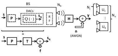
Figure 1: Outline of a quantized massive MU-MIMO broadcast system. Upper diagram: some simplified parts of BS. Lower diagram: Bussgang’s theorem applied to the detached part of interest.

Let us consider the broadcast channel (BC) of a MU-MIMO system with a BS containing $N_{b}$ antennas, which sends radio frequency (RF) signals to users equipped with a total of $N_{u}=\sum_{j=1}^{K}\>N_{j}$ receive antennas, where $N_{j}\geq 1$ denotes the number of receive antennas of the $j$th user $U_{j}$, $j=1,\ldots,K$, as outlined in Fig. 1.

The input-output relation of the BC can be modelled as

$$\mathbf{y}=\mathbf{H}\;\mathbf{s}_{q}\>+\>\mathbf{n},$$ (1)

where $\mathbf{y}\in\mathbb{C}^{N_{u}}$ contains the signals received by all users and $\mathbf{H}\in\mathbb{C}^{N_{u}\times N_{b}}$ stands for the matrix which models the assumed broadcast channel that is assumed known to the BS. The entries of $\mathbf{H}$ are considered independent circularly-symmetrical complex Gaussian random variables $\left[\mathbf{H}\right]_{u,b}\in\mathbb{CN}\left(0,1\right)$, $u=1,\cdots,N_{u}$ and $b=1,\cdots,N_{b}$. The noise vector $\mathbf{n}\in\mathbb{C}^{N_{u}}$ is characterized by its i.i.d. circularly-symmetric complex Gaussian entries $n_{u}\in\mathbb{CN}\left(0,N_{0}\right)$. The noise variance is known at the BS and so is the sampling rate of DACs at BS and ADCs at user equipments. Following the lower part of Fig.1, the quantization $\mathrm{Q}\left(\cdot\right)$ of a precoded symbol vector $\mathbf{Ps}$, where $\mathbf{P}\in\mathbb{C}^{Nb\times Nu}$ is a precoding matrix and $\mathbf{s}\sim\mathbb{CN}\left(\mathbf{0}_{Nu\times 1},\mathbf{I}_{Nu}\right)$ is the symbol vector, can be expressed by the quantized vector given by

$$\mathbf{s}_{q}=\mathrm{Q}\left(\mathbf{Ps}\right)=\mathbf{TPs+f},$$ (2)

where the $\mathbf{f}$ and the symbol $\mathbf{s}$ vectors are uncorrelated. For approximations of achievable sum-rates involving $N_{b}$ and $N_{u}$ sufficiently large, it can be approximated as Gaussian noise, i.e., $\mathbf{f}\in\mathbb{C}^{N_{b}}$.

III Proposed CQA-BD and CQA-RBD Precoding Algorithms

Both proposed ${\scriptstyle\mathrm{CQA-BD}}$ and ${\scriptstyle\mathrm{CQA-RBD}}$ and their respective locally optimized variations ${\scriptstyle\mathrm{CQA-BD-MAAS}}$ and ${\scriptstyle\mathrm{CQA-RBD-MAAS}}$, respectively, are based on ${\scriptstyle\mathrm{BD}}$ and ${\scriptstyle\mathrm{RBD}}$ precoders $\mathbf{P}$ [22, 9, 10, 12, 11, 18] given by

$$\mathbf{P}=\left[\mathbf{P}_{1}\mathbf{P}_{2}\cdots\mathbf{P}_{K}\right]\>\in\mathbb{C}^{N_{b}\times N_{u}}$$ (3)

where the precoding matrices $\mathbf{P}_{j}$ for the jth users can be expressed as the product

$$\mathbf{P}_{j}=\mathbf{P}_{j}^{c}\mathbf{P}_{j}^{d}$$ (4)

where $\mathbf{P}_{j}^{c}\in\mathbb{C}^{N_{b}\times L_{j}}$ and $\mathbf{P}_{j}^{d}\in\mathbb{C}^{L_{j}\times N_{j}}$. The parameter $L_{j}$ depends on which precoding algorithm is chosen, namely, the ${\scriptstyle\mathrm{CQA-BD}}$ or ${\scriptstyle\mathrm{CQA-RBD}}$ techniques.

We can express the combined channel matrix $\mathbf{H}$ and the resulting precoding matrix $\mathbf{P}$ as follows:

$$\mathbf{H}=\left[\mathbf{H}_{1}^{T}\mathbf{H}_{2}^{T}\cdots\mathbf{H}_{K}^{T}\right]^{T}\>\in\mathbb{C}^{N_{u}\times N_{b}}$$ (5)

$$\mathbf{P}=\left[\mathbf{P}_{1}\mathbf{P}_{2}\cdots\mathbf{P}_{K}\right]\>\in\mathbb{C}^{N_{b}\times N_{u}}$$ (6)

where $\mathbf{H}_{j}\in\mathbb{C}^{N_{j}\times N_{b}}$ is the channel matrix of the $j$th user. The matrix $\mathbf{P}_{j}\in\mathbb{C}^{N_{b}\times N_{j}}$ represents the precoding matrix of the $j$th user.

III-A CQA-BD Precoder

In the proposed ${\scriptstyle\mathrm{CQA-BD}}$ precoding algorithm, the first factor in (4) is given by

$$\mathbf{P}_{j}^{c\left(CQA-BD\right)}=\overline{\mathbf{W}}_{j}^{\left(0\right)}$$ (7)

where $\overline{\mathbf{W}}_{j}^{\left(0\right)}$ is obtained by the SVD [12] of (5), in which the channel matrix of the $j$th user has been removed, i.e.:

$$\overline{\mathbf{H}}_{j} =\left[\mathbf{H}_{1}^{T}\cdots\mathbf{H}_{j-1}^{T}\mathbf{H}_{j+1}^{T}\cdots\mathbf{H}_{K}^{T}\right]^{T}\>\in\mathbb{C}^{\overline{N}_{j}\times N_{b}}$$

$$=\overline{\mathbf{U}}_{j}\overline{\mathbf{\Phi}}_{j}\overline{\mathbf{W}}_{j}^{H}=\overline{\mathbf{U}}_{j}\overline{\mathbf{\Phi}}_{j}\left[\overline{\mathbf{W}}_{j}^{\left(1\right)}\overline{\mathbf{W}}_{j}^{\left(0\right)}\right]^{H}$$ (8)

where $\overline{N}_{j}=N_{u}-N_{j}$. The matrix $\overline{\mathbf{W}}_{j}^{\left(0\right)}\in\mathbb{C}^{{N}_{b}\times\left(N_{b}-\overline{L}_{j}\right)}$, where $\overline{L}_{j}$ is the rank of $\overline{\mathbf{H}}_{j}$, uses the last $N_{b}-\overline{L}_{j}$ singular vectors.

The second precoder of ${\scriptstyle\mathrm{CQA-BD}}$ in (4) is obtained by SVD of the effective channel matrix for the $j$th user $\mathbf{H}_{e_{j}}$ and employs a power loading matrix as follows:

$$\mathbf{P}_{j}^{d\left(CQA-BD\right))}=\mathbf{W}_{j}^{\left(1\right)}\>{\left(\mathbf{\Omega}^{\left(CQA-BD\right)}_{j}\right)^{\frac{1}{2}}}$$ (9)

where the power loading matrix $\mathbf{\Omega}^{\left(CQA-BD\right)}_{j}$ requires a power allocation algorithm and the matrix $\mathbf{W}_{j}^{\left(1\right)}$ incorporates the first $\Lambda_{e}=rank\left(\mathbf{H}_{e_{j}}\right)$ singular vectors obtained by the decomposition of $\mathbf{H}_{e_{j}}$, as follows:

$$\mathbf{H}_{e_{j}} =\mathbf{H}_{j}\mathbf{P}_{j}^{c}=\mathbf{U}_{j}\mathbf{\Phi}_{j}\mathbf{W}_{j}^{H}$$

$$=\mathbf{U}_{j}\begin{bmatrix}\mathbf{\Phi}_{j}&0\\ 0&0\end{bmatrix}\begin{bmatrix}\mathbf{W}_{j}^{\left(1\right)}&\mathbf{W}_{j}^{\left(0\right)}\end{bmatrix}^{H}$$ (10)

III-B CQA-RBD Precoder

In the case of the proposed ${\scriptstyle\mathrm{CQA-RBD}}$ precoding algorithm, the first precoder in (4) is given [10, 12] by

$$\mathbf{P}_{j}^{c\left(CQA-RBD\right)}=\overline{\mathbf{W}}_{j}\left(\overline{\mathbf{\Phi}}_{j}^{T}\overline{\mathbf{\Phi}_{j}}+{\chi}\;\mathbf{I}_{N_{b}}\right)^{-1/2}$$ (11)

where $\chi=\frac{N_{u}\sigma_{n}^{2}}{P}$ is the regularization factor required by the ${\scriptstyle\mathrm{CQA-RBD}}$ algorithm and $P$ is the average transmit power.

The second precoder of ${\scriptstyle\mathrm{CQA-RBD}}$ in (4) is obtained by SVD of the effective channel matrix for the $j$th user $\mathbf{H}_{e_{j}}$ and power loading, respectively as follows:

$$\mathbf{P}_{j}^{d\left(CQA-RBD\right))}=\mathbf{W}_{j}\>{\left(\mathbf{\Omega}^{\left(CQA-RBD\right)}_{j}\right)^{\frac{1}{2}}}$$ (12)

where the matrix $\mathbf{W}_{j}^{\left(1\right)}$ incorporates the early $\Lambda_{e}=rank\left(\mathbf{H}_{e_{j}}\right)$ singular vectors obtained by the decomposition of $\mathbf{H}_{e_{j}}$, as follows:

$$\mathbf{H}_{e_{j}} =\mathbf{H}_{j}\mathbf{P}_{j}^{c}=\mathbf{U}_{j}\mathbf{\Phi}_{j}\mathbf{W}_{j}^{H}$$

$$=\mathbf{U}_{j}\begin{bmatrix}\mathbf{\Phi}_{j}&0\\ 0&0\end{bmatrix}\begin{bmatrix}\mathbf{W}_{j}^{\left(1\right)}&\mathbf{W}_{j}^{\left(0\right)}\end{bmatrix}^{H}$$ (13)

The power loading matrix per user $\mathbf{\Omega}_{j}^{\left(CQA-RBD\right)}$ can be obtained by a procedure like water filling (WF) [26] power allocation and will be initialized with equal power allocation.

The quantized vector (2) combined with the asumptions that $\left(\mathit{N}_{b},\>\mathit{N}_{u}\right)$ is sufficiently large and that the quantization error from DACs is Gaussian lead [18] to the following transmit processing matrix:

$$\mathbf{T}_{n,n}=\delta\>\mathbf{I}_{Nb\times Nb},$$ (14)

where the scalar factor is described by

$$\delta=\alpha\gamma\sqrt{\frac{N_{b}}{\pi P}}\sum_{l=1}^{J-1}\exp\left(-\frac{N_{b}\gamma^{2}}{P}\left(1-\frac{J}{2}\right)^{2}\right)\,$$ (15)

which concentrates all process of quantization on the scalar $\delta$ in (14) and is used to compute the sum-rates at the receiver. The losses of achievable sum-rates for a fixed SNR due to the coarse quantization and a fixed realization of the channel are fully characterized by $\mathbf{T}_{n,n}$. The steps needed to compute ${\scriptstyle\mathrm{CQA-BD}}$ and ${\scriptstyle\mathrm{CQA-RBD}}$ are summarized in Algorithm 1.

Algorithm 1 Proposed CQA-BD and CQA-RBD precoders

1:$\begin{aligned} \alpha&=\left(2\mathrm{N_{b}}\gamma^{2}\left(\left(\frac{J-1}{2}\right)^{2}\right.\right.\\ &\left.\left.-2\sum_{l=1}^{J-1}\left(1-\frac{J}{2}\right)\Xi\left(\sqrt{2N_{b}\gamma^{2}}\left(1-\frac{J}{2}\right)\right)\right)\right)^{-1/2}\eqref{normalization_factor}\end{aligned}$ $\begin{aligned} \delta=\alpha\gamma\sqrt{\frac{N_{b}}{\pi P}}\sum_{l=1}^{J-1}\exp\left(-\frac{N_{b}\gamma^{2}}{P}\left(1-\frac{J}{2}\right)^{2}\right)\eqref{entries_diag_mat_dist}\end{aligned}$ $\begin{aligned} \mathbf{H}=\left[\mathbf{H}_{1}^{T}\mathbf{H}_{2}^{T}\cdots\mathbf{H}_{K}^{T}\right]^{T}\>\in\mathbb{C}^{N_{u}\times N_{b}}\>\eqref{comb_ch_matrix}\end{aligned}$

2:for $\mathrm{j=1\;}\colon\>K$ do

3:    $\overline{\mathbf{H}}_{j}=\left[\mathbf{H}_{1}^{T}\cdots\mathbf{H}_{j-1}^{T}\mathbf{H}_{j+1}^{T}\cdots\mathbf{H}_{K}^{T}\right]^{T}\>\in\mathbb{C}^{\overline{N}_{j}\times N_{b}}$(III-A)

4:    $\overline{\mathbf{H}}_{j}=\overline{\mathbf{U}}_{j}\overline{\mathbf{\Phi}}_{j}\overline{\mathbf{W}}_{j}^{H}=\overline{\mathbf{U}}_{j}\overline{\mathbf{\Phi}}_{j}\left[\overline{\mathbf{W}}_{j}^{\left(1\right)}\overline{\mathbf{W}}_{j}^{\left(0\right)}\right]^{H}$ (III-A)

5:    $\mathbf{P}_{j}^{c\left(CQA-BD\right)}=\overline{\mathbf{W}}_{j}^{\left(0\right)}$(7)

6:    $\mathbf{P}_{j}^{c\left(RBD\right)}=\overline{\mathbf{W}}_{j}\left(\overline{\mathbf{\Phi}}_{j}^{T}\overline{\mathbf{\Phi}}_{j}+{\chi}\>\mathbf{I}_{N_{b}}\right)^{-1/2}$(11)

7:    $\mathbf{H}_{e_{j}}=\mathbf{H}_{j}\mathbf{P}_{j}^{c}=\mathbf{U}_{j}\mathbf{\Phi}_{j}\mathbf{W}_{j}^{H}=\mathbf{U}_{j}\begin{bmatrix}\mathbf{\Phi}_{j}&0\\ 0&0\end{bmatrix}\begin{bmatrix}\mathbf{W}_{j}^{\left(1\right)}&\mathbf{W}_{j}^{\left(0\right)}\end{bmatrix}^{H}$(III-A)

8:    $\left(\mathbf{\Omega}^{\left(CQA-BD,CQA-RBD\right)}_{j}\right)^{\frac{1}{2}}$ by classical WF [26] or variations

9:    $\mathbf{P}_{j}^{d\left(CQA-BD\right))}=\mathbf{W}_{j}^{\left(1\right)}\>{\left(\mathbf{\Omega}^{\left(BD\right)}_{j}\right)^{\frac{1}{2}}}$ (9)

10:    $\mathbf{P}_{j}^{d\left(CQA-RBD\right))}=\mathbf{W}_{j}\>{\left(\mathbf{\Omega}^{\left(CQA-RBD\right)}_{j}\right)^{\frac{1}{2}}}$ (12)

11:    $\mathbf{P}_{j}=\mathbf{P}_{j}^{c}\mathbf{P}_{j}^{d}$ (4)

12:end for

13:$\mathbf{P}=\left[\mathbf{P}_{1}\mathbf{P}_{2}\cdots\mathbf{P}_{K}\right]^{T}\>\in\mathbb{C}^{N_{b}\times N_{u}}$ (6)

Extensions to other precoders and/or beamforming strategies [30, 28, 29, 31, 32, 33, 34, 35, 37, 38, 36, 44, 40, 39, 41, 42, 43, 45, 46, 47] are possible. Moreover, detection and parameter estimation strategies can also be considered for future work [58, 59, 60, 61, 62, 63, 64, 65, 66, 57, 67].

IV Proposed CQA-MAAS Power Allocation

The achievable rate [17] in bits per channel use at which information can be sent with arbitrarily low probability of error can be bounded by the mutual information of a Gaussian channel [50, 19, 17] as follows:

$$\mathit{C}\leq \mathit{I}\left(\mathbf{s},\mathbf{y}\>\right)=\log_{2}\left\{\det\left[\mathbf{I}_{Nu}+\frac{\mathit{SNR}}{\mathit{N}_{u}}\mathbf{\left(HP\right)}\mathbf{\left(HP\right)}^{H}\right.\right.$$

$$\left.\left.\left(\left(1-\delta^{2}\right)\frac{\mathit{SNR}}{\mathit{N}_{u}}\mathbf{\left(HP\right)}\mathbf{\left(HP\right)}^{H}+\mathbf{I}_{Nu}\right)^{-1}\right]\right\}$$ (16)

where the scalar factor $\delta$ concentrates the quantization impact.

The proposed CQA-MAAS power allocation involves appproximations of Neumann’s (matrix), EVD and SVD in addition to other properties [21, 23], which allow us to formulate [18] it as a conditioned maximization process of the achievable sum rate (IV), as follows:

$$\mathit{C} \approx\max_{\Phi_{j}}\sum_{j=1}^{K}\log_{2}\bigg{|}\mathbf{I}_{N_{j}}+\frac{\delta^{2}}{\mathrm{N}_{0}}\>\mathbf{\Phi}_{j}^{2}\>\mathbf{\Omega}_{j}-\frac{\delta^{2}\left(1-\delta^{2}\right)}{\mathrm{N}_{0}^{2}}\>\mathbf{\Phi}_{j}^{4}\>\mathbf{\Omega}_{j}^{2}\bigg{|}$$

$$=\max_{\Phi_{j}}\sum_{j=1}^{K}\mathrm{Tr}\left[\mathrm{\log}_{2}\bigg{|}\mathbf{I}_{N_{j}}+\frac{\delta^{2}}{\mathrm{N}_{0}}\>\mathbf{\Phi}_{j}^{2}\>\mathbf{\Omega}_{j}\right.$$

$$\left.-\frac{\delta^{2}\left(1-\delta^{2}\right)}{\mathrm{N}_{0}^{2}}\>\mathbf{\Phi}_{j}^{4}\>\mathbf{\Omega}_{j}^{2}\bigg{|}\right]$$

$$\qquad\mathrm{s.t.}\sum_{j=1}^{K}\mathrm{Tr}\left(\mathbf{\Omega}_{j}\right)\leq\>\mathit{P}_{total}$$ (17)

where $\mathbf{\Phi}_{j}$ and $\mathbf{\Omega}_{j}$ are estimated by the SVD of the non-interfering block channels (III-A) for ${\scriptstyle\mathrm{CQA-BD-MAAS}}$ and (III-B) for ${\scriptstyle\mathrm{CQA-RBD-MAAS}}$.

The optimized precoding matrix for ${\scriptstyle\mathrm{BD}}$ algorithm $\mathbf{P}_{opt}$ makes use of a conditioned maximization process of the achievable sum rate and involves appproximations of Neumann’s (matrix) and Mc Laurin’s series [21, 23]. It is computed at each realization of the channel by incorporation of the power loading effects of diagonal matrices $\Omega_{j}$, $j=1,\ldots,K$, corresponding to the $N_{j}$ antennas of each $j$th user as follows:

$$\mathbf{P}_{opt}^{BD} =\left[\overline{\mathbf{W}}_{1}^{\left(0\right)}\mathbf{W}_{1}^{\left(1\right)}\>\left(\mathbf{\Omega}^{\left(BD\right)}_{1}\right)^{\frac{1}{2}}\cdots\overline{\mathbf{W}}_{K}^{\left(0\right)}\mathbf{W}_{K}^{\left(1\right)}\>\left(\mathbf{\Omega}^{\left(BD\right)}_{K}\right)^{\frac{1}{2}}\right]$$

$$=\left[\overline{\mathbf{W}}_{1}^{\left(0\right)}\mathbf{W}_{1}^{\left(1\right)}\cdots\overline{\mathbf{W}}_{K}^{\left(0\right)}\mathbf{W}_{K}^{\left(1\right)}\right]\>\left(\mathbf{\Omega}^{\left(BD\right)}\right)^{\frac{1}{2}}$$ (18)

where $\mathbf{\Omega}^{\left(BD\right)}$ is a larger power diagonal matrix, where each of its $\mathrm{Nu}$ entries is associated to its corresponding $\mathit{j}$th user, in ascending order, as follows:

$$\mathbf{\Omega}^{\left(BD\right)}=\mathrm{diag}\{\mathbf{\Omega}_{1},\cdots,\mathbf{\Omega}_{K}\},$$ (19)

which can be detailed as follows:

$$\mathbf{\Omega}^{\left(BD\right)}=\begin{bmatrix}\omega_{1}&\cdots&0&\cdots\cdots&0&\cdots&0\\ \vdots&\ddots&\vdots&&\vdots&\ddots&\vdots\\ 0&\underbrace{\cdots}_{\mathbf{\Omega}_{1}}&\omega_{Nj}&\cdots\cdots&0&\cdots&0\\ \vdots&&\vdots&\ddots&\vdots&&\vdots\\ \vdots&&\vdots&&\vdots&&\vdots\\ 0&\cdots&0&\cdots\cdots&\omega_{\left(\mathrm{N_{u}}-Nj\right)}&\cdots&0\\ \vdots&\ddots&\vdots&&\vdots&\ddots&\vdots\\ 0&\cdots&0&\cdots\cdots&0&\underbrace{\cdots}_{\mathbf{\Omega}_{K}}&\omega_{\mathit{\left(N_{u}=K\times Nj\right)}}\end{bmatrix}$$ (20)

The computation of $\mathbf{\Omega}^{\left(BD\right)}$ is based on a locally optimized level of energy $\mu_{opt}$ (IV)

$$\mu_{opt} =\frac{\left(\mathit{N}_{u}-\mathit{p}+1\right)^{2}}{2\mathit{C}_{2}\mathrm{SNR}\sum_{m=1}^{\left(\mathit{N}_{u}-\mathit{p}+1\right)}\left[\phi^{2}\right]_{m}}$$

$$\times\Bigg{\{}1-\left[1+\frac{4\mathit{C}_{2}}{\mathit{N}_{u}^{2}}\sum_{m=1}^{\left(\mathit{N}_{u}-\mathit{p}+1\right)}\left[\phi^{2}\right]_{m}\right.$$

$$\times\left.\left(-\mathrm{SNR}\>+\mathit{C}_{1}\sum_{m=1}^{\left(\mathit{N}_{u}-\mathit{p}+1\right)}\left[\frac{1}{\phi^{2}}\right]_{m}\right)\right]^{\frac{1}{2}}\Bigg{\}},$$ (21)

where

1. $\mathit{N}_{u}$ stands for the number of receive antennas defined in Section II.

2. $\mathit{p}$ denotes an auxiliary parameter to be set to $1$.

3. $\mathit{C}_{1}$ and $\mathit{C}_{2}$, which depend only on the distortion factor $\delta$, are given by (22) and (23).

   $$\mathit{C}_{1}=\frac{\delta-\sqrt{4-3\delta^{2}}}{2\delta\left(1-\delta^{2}\right)}$$ (22)

   $$\mathit{C}_{2}=\frac{\delta\left(1-\delta^{2}\right)}{\sqrt{4-3\delta^{2}}}$$ (23)

4. $\phi$ designates each of the $\mathrm{N}_{u}=\mathit{K\times N_{j}}$ singular values corresponding to each receive antenna. This can be better visualized in the following diagonal matrix (LABEL:Diag_sv_matrix), in which the diagonal vector displays the required entries $\phi_{m}$ $\in$ $\phi_{1},\cdots,\phi_{\mathit{N_{u}}}$ .

Employing the value of $\mu_{opt}$ provided by (IV), the power allocated to the $\mathit{m}$th $\in$ $\{1,\cdots,\mathrm{N_{u}}\}$ receive antenna can be computed by

$$\omega_{m} =\mathit{C}_{1}\frac{\left(\mathit{N}_{u}-\mathit{p}+1\right)}{\mathrm{SNR}}\>\frac{1}{\phi^{2}_{m}}+\mu_{opt}$$

$$-\mu^{2}_{opt}\mathit{C}_{2}\frac{\mathrm{SNR}}{\left(\mathit{N}_{u}-\mathit{p}+1\right)}\>\phi^{2}_{m}$$ (24)

where the parameters involved were defined in (i), (ii), (iii) and (iv). Assuming that the power alloted to the receive antenna which is associated to the minimum gain is negative, i.e., $\omega_{\mathit{N}_{u}-\mathit{p}+1}<0$, it is rejected, and the algorithm must be executed with the parameter $\mathit{p}$ increased by unity. The most advantageous allotment strategy is achieved at the time that the power distributed among each receive antenna is non-negative according to the Khun-Tucker conditions (25):

$$\left.\left(\omega_{nn}\right)^{+}\right|_{nn=1,...,N_{u}}=\omega, \mathrm{if}\>\omega_{nn}\geq 0$$

$$0, \mathrm{if}\>\omega_{nn}<0$$ (25)

The proposed ${\scriptstyle\mathrm{CQA-MAAS}}$ power allocation can be summed up as in Algorithm (2), as follows:

Algorithm 2 Proposed CQA-MAAS power allocation

1:$\mathbf{Initialization}:\mathrm{Nu},\mathrm{Nb},\mathit{K}$

2:

$$\mathbf{\Phi}=\begin{bmatrix}\phi_{1}&\cdots&0\\ \vdots&\ddots&\vdots\\ 0&\cdots&\phi_{\mathit{N_{u}}}\end{bmatrix}\eqref{Diag_sv_matrix}$$

3:$\mathbf{Compute}$ the factors $\mathit{C}_{1}$ in (22) and $\mathit{C}_{2}$ in (23).

4:$\mathbf{Compute}$ the optimum energy level $\mu_{opt}$ in (IV).

5:$\mathbf{Compute}$ the power allocation to each sub-channel $\omega_{m}$ in (IV).

6:$\mathbf{If}$ there are negative values, then find their minimum, i.e., their $\min\left(\omega_{N_{u}-p+1}<0\right)$ $\mathbf{and}$.

7:$\mathbf{Refuse}$ this minimum negative value by assuming it is equal to zero in (25), $\mathbf{and}$.

8:$\mathbf{Perform}$ the algorithm with the parameter $\mathit{p}$ incremented by unity.

9:CQA-MAAS achieves its goal when the power allocated among the receive antennas is non-negative (25).

10:$\mathbf{Compute}$ the power diagonal matrix (20), by relating its $N_{u}$ power entries to their corresponding receive antennas.

V Numerical results

We consider two scenarios with a MU-MIMO system using $N_{b}=64$ and $N_{u}=16\times 2$ and$N_{b}=64$ and $N_{u}=8\times 2$ that assume the conditions described in Section II. Fig.2 employs the firsf scenario in order to illustrate the achievable sum-rates for the proposed ${\scriptstyle\mathrm{CQA-BD-MAAS}}$, which results from coarse-quantization most advantageous allocation strategy (${\scriptstyle\mathrm{CQA-MAAS}}$) power allocation algorithm to block-diagonalization precoding for 2, 3 and 4-bit quantization. They are compared to BD full resolution ${\scriptstyle\mathrm{BD-FR}}$ and its existing variant ${\scriptstyle\mathrm{BD-FR\>plus\>existing\>Waterfilling}}$ [22]. Considering the influence of practical aspects, we have modeled an imperfect channel knowledge combined with a spatial correlation $\hat{\mathbf{H}}=\mathbf{H}\;\tilde{\mathbf{R}}\ ^{\frac{1}{2}}+\mathbf{E}$, where $\tilde{\mathbf{R}}$ represents the complex transmit correlation matrix [55, 12] whose elements are

$$\tilde{R}_{ij}=\left\{\begin{array}[]{ll}r^{j-i},&i\leq j\\ r_{ji}^{*},&i>j\end{array}\right.,|r|\leq 1$$ (28)

where $\lvert\mathrm{r}\rvert<1$. It can be noticed that the absolute values of the entries $\lvert\tilde{\mathrm{R}}_{\left(i,j\right)}\rvert$ corresponding to the closest antennas are larger than the others. The error matrix $\mathbf{E}$ is modeled [12] as a complex Gaussian noise with i.i.d entries of zero mean and variance $\sigma_{e}^{2}$. In our next examples, we have employed large values of correlations between the neighboring antennas, i.e., $\lvert\mathrm{r}\rvert=0.72$ and $0.91$, respectively. The variance $\sigma_{e}^{2}$ of the feedback error matrix $\mathbf{E}$ has been set to $0.16$.

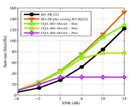
Figure 2: Achievable rates for CQA-BD-MAAS, $2,3,4,$ quantization bits, via Bussgang theorem, Gaussian signals, compared to BD-FR and BD-FR-plus existing WF. MU-MIMO configuration: $N_{b}=64$ and $N_{u}=16\times 2$.

In Fig. 3, in which the scenario is composed with $N_{b}=64$ and $N_{u}=8\times 2$, we assess the performance of ${\scriptstyle\mathrm{CQA-BD}}$ and ${\scriptstyle\mathrm{CQA-BD-MAAS}}$ in the presence of imperfect channel knowledge and spatial correlation using $3$ and $6$ bits. The results show that the impact of imperfect channel knowledge is not significant in terms of performance degradation of the precoders. However, the performance degradation of ${\scriptstyle\mathrm{CQA-BD-MAAS}}$ can become significant for $3$ bits.

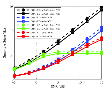
Figure 3: Achievable rates for CQA-BD and CQA-BD-MAAS for 6 and 3-bit quantization under perfect and imperfect channel knowledge (ICH). MU-MIMO configuration: $N_{b}=64$ and $N_{u}=8\times 2$. $\lvert\mathrm{r}\rvert=0.72$ and $\sigma_{e}^{2}=0.16$.

.

The number of FLOPs required by conventional ${\scriptstyle\mathrm{BD}}$ and ${\scriptstyle\mathrm{RBD}}$ algorithms are dominated by two SVDs [22]. Since our system model is dedicated to broadcast channels, we can assume the widespread ratios $N_{b}\gg N_{u}\gg N_{j}$ and one of their resulting approximations $N_{u}-N_{j}\approx N_{u}$ to simplify the resulting expressions. Table I illustrates the computational cost required by the proposed ${\scriptstyle\mathrm{CQA}}$ and existing precoders.

TABLE I: Computational complexity of BD, RBD and their proposed coarsely quantized variations based on Bussgang Theorem: CQA-BD and CQA-RBD

Precoder	Computational cost (FLOPs) under $N_{b}\gg N_{u}\gg N_{j}$
BD	${N_{b}^{2}}\left(32N_{j}+8\right)+N_{b}\left(32N_{u}^{2}+72N_{j}^{2}\right)+64N_{u}^{2}$
RBD	${N_{b}^{2}}\left(32N_{j}+8\right)+N_{b}\left(32N_{u}^{2}+72N_{j}^{2}\right)+64N_{u}^{2}$
Proposed	${N_{b}^{2}}\left(32N_{j}+8\right)+N_{b}\left(32N_{u}^{2}+72N_{j}^{2}\right)+64N_{u}^{2}+C_{\delta}$
CQA-BD
Proposed	${N_{b}^{2}}\left(32N_{j}+8\right)+N_{b}\left(32N_{u}^{2}+72N_{j}^{2}\right)+64N_{u}^{2}+C_{\delta}$
CQA-RBD

The extra cost $C_{\delta}$ required to convert ${\scriptstyle\mathrm{BD}}$ and ${\scriptstyle\mathrm{RBD}}$ into their corresponding Bussgang-based precoders, which are listed in Table I, do not have significant impact on the total computational cost of their respective Bussgang-based algorithms. Due to their design, existing waterfilling and the proposed CQA-MAAS power allocation have a similar computational cost of $\mathcal{O}\left(N_{u}\right)$, which in practice does not result in significant additional cost to be imposed on ${\scriptstyle\mathrm{BD}}$ and ${\scriptstyle\mathrm{RBD}}$ to obtain their respective ${\scriptstyle\mathrm{CQA-BD-MAAS}}$ and ${\scriptstyle\mathrm{CQA-RBD-MAAS}}$ schemes. Table (II) summarizes these additional costs.

TABLE II: Computational complexity of proposed CQA-MAAS and existing WF algorithms.

Technique	Computational cost (FLOPs)
Waterfilling (WF)	$\mathcal{O}\left(N_{u}\right)$
MAAS	$\mathcal{O}\left(N_{u}\right)$

VI Conclusion

We have investigated ${\scriptstyle\mathrm{CQA-BD}}$ and ${\scriptstyle\mathrm{CQA-RBD}}$ precoding and developed the ${\scriptstyle\mathrm{CQA-RBD-MAAS}}$ power allocation algorithms for large-scale MIMO systems that employ coarse quantization using DACs with few bits. ${\scriptstyle\mathrm{CQA-RBD-MAAS}}$ can obtain gains in sum-rate of up to $30$ % over schemes without power allocation and comparable performance to full-resolution schemes with precoding and WF power allocation. The proposed algorithms can be used in massive MIMO systems and contribute to substantial reduction in power consumption.

References

- [1] Landau, L, T. N., Lamare, R. C., ’Branch-and-Bound Precoding for Multiuser MIMO Systems With 1-Bit Quantization’, IEEE Wireless Communications Letters, 6,(6), Dec. 2017
- [2] Mezghani, A., Ghiat, R., Nossek, J. A., ’Transmit processing with low resolution D/A-converters’, 16th IEEE International Conference on Electronics, Circuits and Systems, pp.1-4, 2009.
- [3] Bussgang, J.J., ’Crosscorrelation functions of amplitude-distorted Gaussian signals’, Res. Lab. Elec., Cambridge, MA, USA, Tech. Rep. 216, Mar. 1952.
- [4] Jacobsson, S., Durisi, G., Coldrey, M., Goldstein,T., Studer, C., ’Quantized precoding for massive MU-MIMO’, IEEE Trans. on Communications, 65, (11), Nov. 2017.
- [5] Jacobsson, S., Durisi, G., Coldrey, M., Gustavsson, U., Studer, C., ’Throughput Analysis of Massive MIMO Uplink With Low-Resolution ADCs’, IEEE Transactions on Wireless Communications, 16 , (6) , Jun. 2017.
- [6] Jacobsson, S., Durisi, G., Coldrey, M., Studer, C., ’Linear Precoding With Low-Resolution DACs for Massive MU-MIMO-OFDM Downlink’, IEEE Transactions on Wireless Communications, 18 , (3) , Mar. 2019.
- [7] Rowe, H., ’Memoryless nonlinearities with Gaussian inputs: Elementary results’, Bell System Technical Journal, 61, (7), pp.1519-1525, Sep. 1982.
- [8] Paulraj, A., Nabar, R., Gore, D., ’Introduction to Space-Time Wireless Communications’, Cambridge University Press
- [9] Sung, H., Lee, S., Lee, I., ’Generalized Channel Inversion Methods for Multiuser MIMO Systems’, IEEE Transactions on Communications, 57, (11), Nov. 2009.
- [10] Stankovic, V., Haardt, M., ’Generalized Design of Multi-User MIMO Precoding Matrices’, IEEE Transactions on Wireles Communications, 7, (3), Mar. 2008.
- [11] Zu, K. and de Lamare R. C., ’Low-Complexity Lattice Reduction-Aided Regularized Block Diagonalization for MU-MIMO Systems,’ IEEE Communications Letters, vol. 16, no. 6, pp. 925-928, June 2012.
- [12] Zu, K., Lamare, R. C., and Haardt, M., ’Generalized Design of Low-Complexity Block Diagonalization Type Precoding Algorithms for Multiuser MIMO Systems’, IEEE Transactions on Communications, 61, (10), Oct. 2013.
- [13] Zhang, W. et al., ’Widely Linear Precoding for Large-Scale MIMO with IQI: Algorithms and Performance Analysis,’ IEEE Transactions on Wireless Communications, vol. 16, no. 5, pp. 3298-3312, May 2017.
- [14] Wei Yu, Wonjong Rhee, S. Boyd and J. M. Cioffi, ’Iterative water-filling for Gaussian vector multiple-access channels,’ IEEE Transactions on Information Theory, vol. 50, no. 1, pp. 145-152, Jan. 2004.
- [15] Palomar, D.P., Fonollosa, J. R., ’Practical Algorithms for a Family of Waterfilling Solutions’, IEEE Transactions on Signal Processing, 53, (2), Feb. 2005.
- [16] Khan, M.H.A., Cho, K.M., Lee, M.H. et al. ,’A simple block diagonal precoding for multi-user MIMO broadcast channels’, J Wireless Com Network, 95, 2014.
- [17] Pinto, S. F. B., and de Lamare, R.C., “ Quantization-Aware Block Diagonalization Algorithms for Multiple-Antenna Systems with Low-Resolution Signals’, 24th International ITG Workshop on Smart Antennas, pp.1-6, Hamburg, Germany, Feb.2020.
- [18] Pinto, S. F. B. Pinto and de Lamare, R. C., Block Diagonalization Precoding and Power Allocation for Multiple-Antenna Systems with Coarsely Quantized Signals July 2021 IEEE Transactions on Communications, pp.99:1-1
- [19] Telatar, I. E., ’Capacity of Multi-Antenna Gaussian Channels’, Rm.2C-174, Lucent Technologies, Bell Laboratories, 1999.
- [20] Cover, T.H., Thomas, J. A., ’Elements of Information Theory’, Second Edition, Wiley, 2006.
- [21] Seber, G. A. F., ’A Matrix Handbook for Statisticians’, Wiley, 2008., 2003.
- [22] Spencer, Q. H. , Swindlehurst, A. L. and Haardt, M., ”Zero-forcing methods for downlink spatial multiplexing in multiuser MIMO channels,” in IEEE Transactions on Signal Processing, vol. 52, no. 2, pp. 461-471, Feb. 2004.
- [23] Harville, D.A.,’Matrix Algebra From a Statistician’s Perspective’, Springer 1997.
- [24] Loyka, S. L., ’Channel capacity of MIMO architecture using the exponential correlation matrix’, IEEE Communications Letters, vol.5, no. 9, pp. 369-371, Sept. 2001.
- [25] Zhang, W. et al., ’Widely Linear Precoding for Large-Scale MIMO with IQI: Algorithms and Performance Analysis,’ IEEE Transactions on Wireless Communications, vol. 16, no. 5, pp. 3298-3312, May 2017.
- [26] Paulraj, A., Nabar, R., Gore, D., ’Introduction to Space-Time Wireless Communications’, Cambridge University Press, 2003.
- [27] S. F. B. Pinto and R. C. de Lamare, “Block Diagonalization Precoding and Power Allocation for Multiple-Antenna Systems with Coarsely Quantized Signals”, IEEE Transactions on Communications, 2021.
- [28] L. T. N. Landau, M. Dorpinghaus, R. C. de Lamare and G. P. Fettweis, ”Achievable Rate With 1-Bit Quantization and Oversampling Using Continuous Phase Modulation-Based Sequences,” in IEEE Transactions on Wireless Communications, vol. 17, no. 10, pp. 7080-7095, Oct. 2018.
- [29] Z. Shao, L. T. N. Landau and R. C. de Lamare, ”Dynamic Oversampling for 1-Bit ADCs in Large-Scale Multiple-Antenna Systems,” in IEEE Transactions on Communications, vol. 69, no. 5, pp. 3423-3435, May 2021
- [30] W. Zhang et al., ”Large-Scale Antenna Systems With UL/DL Hardware Mismatch: Achievable Rates Analysis and Calibration,” in IEEE Transactions on Communications, vol. 63, no. 4, pp. 1216-1229, April 2015.
- [31] Y. Cai, R. C. d. Lamare and R. Fa, ”Switched Interleaving Techniques with Limited Feedback for Interference Mitigation in DS-CDMA Systems,” in IEEE Transactions on Communications, vol. 59, no. 7, pp. 1946-1956, July 2011
- [32] Y. Cai, R. C. de Lamare and D. Le Ruyet, ”Transmit Processing Techniques Based on Switched Interleaving and Limited Feedback for Interference Mitigation in Multiantenna MC-CDMA Systems,” in IEEE Transactions on Vehicular Technology, vol. 60, no. 4, pp. 1559-1570, May 2011
- [33] Y. Cai, R. C. de Lamare, L. Yang and M. Zhao, ”Robust MMSE Precoding Based on Switched Relaying and Side Information for Multiuser MIMO Relay Systems,” in IEEE Transactions on Vehicular Technology, vol. 64, no. 12, pp. 5677-5687, Dec. 2015.
- [34] X. Lu and R. C. d. Lamare, ”Opportunistic Relaying and Jamming Based on Secrecy-Rate Maximization for Multiuser Buffer-Aided Relay Systems,” in IEEE Transactions on Vehicular Technology, vol. 69, no. 12, pp. 15269-15283, Dec. 2020
- [35] V. M. T. Palhares, A. R. Flores and R. C. de Lamare, ”Robust MMSE Precoding and Power Allocation for Cell-Free Massive MIMO Systems,” in IEEE Transactions on Vehicular Technology, vol. 70, no. 5, pp. 5115-5120, May 2021
- [36] A. R. Flores, R. C. de Lamare and B. Clerckx, ”Linear Precoding and Stream Combining for Rate Splitting in Multiuser MIMO Systems,” in IEEE Communications Letters, vol. 24, no. 4, pp. 890-894, April 2020,
- [37] K. Zu, R. C. de Lamare and M. Haardt, ”Multi-Branch Tomlinson-Harashima Precoding Design for MU-MIMO Systems: Theory and Algorithms,” in IEEE Transactions on Communications, vol. 62, no. 3, pp. 939-951, March 2014.
- [38] L. Zhang, Y. Cai, R. C. de Lamare and M. Zhao, ”Robust Multibranch Tomlinson–Harashima Precoding Design in Amplify-and-Forward MIMO Relay Systems,” in IEEE Transactions on Communications, vol. 62, no. 10, pp. 3476-3490, Oct. 2014,
- [39] S. D. Somasundaram, N. H. Parsons, P. Li and R. C. de Lamare, ”Reduced-dimension robust capon beamforming using Krylov-subspace techniques,” in IEEE Transactions on Aerospace and Electronic Systems, vol. 51, no. 1, pp. 270-289, January 2015.
- [40] N. Song, W. U. Alokozai, R. C. de Lamare and M. Haardt, ”Adaptive Widely Linear Reduced-Rank Beamforming Based on Joint Iterative Optimization,” in IEEE Signal Processing Letters, vol. 21, no. 3, pp. 265-269, March 2014
- [41] H. Ruan and R. C. de Lamare, ”Robust Adaptive Beamforming Using a Low-Complexity Shrinkage-Based Mismatch Estimation Algorithm,” in IEEE Signal Processing Letters, vol. 21, no. 1, pp. 60-64, Jan. 2014
- [42] H. Ruan and R. C. de Lamare, ”Robust Adaptive Beamforming Based on Low-Rank and Cross-Correlation Techniques,” in IEEE Transactions on Signal Processing, vol. 64, no. 15, pp. 3919-3932, 1 Aug.1, 2016
- [43] H. Ruan and R. C. de Lamare, ”Distributed Robust Beamforming Based on Low-Rank and Cross-Correlation Techniques: Design and Analysis,” in IEEE Transactions on Signal Processing, vol. 67, no. 24, pp. 6411-6423, 15 Dec.15, 2019
- [44] A. R. Flores, R. C. De Lamare and B. Clerckx, ”Tomlinson-Harashima Precoded Rate-Splitting With Stream Combiners for MU-MIMO Systems,” in IEEE Transactions on Communications, vol. 69, no. 6, pp. 3833-3845, June 2021.
- [45] T. Peng, R. C. de Lamare and A. Schmeink, ”Adaptive Distributed Space-Time Coding Based on Adjustable Code Matrices for Cooperative MIMO Relaying Systems,” in IEEE Transactions on Communications, vol. 61, no. 7, pp. 2692-2703, July 2013
- [46] J. Gu, R. C. de Lamare and M. Huemer, ”Buffer-Aided Physical-Layer Network Coding With Optimal Linear Code Designs for Cooperative Networks,” in IEEE Transactions on Communications, vol. 66, no. 6, pp. 2560-2575, June 2018
- [47] Y. Jiang et al., ”Joint Power and Bandwidth Allocation for Energy-Efficient Heterogeneous Cellular Networks,” in IEEE Transactions on Communications, vol. 67, no. 9, pp. 6168-6178, Sept. 2019.
- [48] Naber, J., Singh, H. , Sadler, R., Milan, J., ’A low-power, high-speed 4-bit GAAS ADC and 5-bit DAC’, Proc. 11th Annu. Gallium Arsenide Integr. Circuit Symp., San Diego, CA, USA, pp.333-336, Oct. 1989.
- [49] Orhan, O., Erkip, E., Rangan, S., ’Low power analog-to-digital converter in millimiter wave systems: Impact of resolution and bandwidth on performance’, Information theory and Applications Workshop, pp. 191-198, Feb.2015.
- [50] Cover, T.H., Thomas, J. A., ’Elements of Information Theory’, Second Edition, Wiley, 2006.
- [51] Wei Yu, Wonjong Rhee, S. Boyd and J. M. Cioffi, ’Iterative water-filling for Gaussian vector multiple-access channels,’ IEEE Transactions on Information Theory, vol. 50, no. 1, pp. 145-152, Jan. 2004.
- [52] Palomar, D.P., Fonollosa, J. R., ’Practical Algorithms for a Family of Waterfilling Solutions’, IEEE Transactions on Signal Processing, 53, (2), Feb. 2005.
- [53] Khan, M.H.A., Cho, K.M., Lee, M.H. et al. ,’A simple block diagonal precoding for multi-user MIMO broadcast channels’, J Wireless Com Network, 95, 2014.
- [54] Bussgang, J.J., ’Crosscorrelation functions of amplitude-distorted Gaussian signals’, Res. Lab. Elec., Cambridge, MA, USA, Tech. Rep. 216, Mar. 1952.
- [55] Loyka, S. L., ’Channel capacity of MIMO architecture using the exponential correlation matrix’, IEEE Communications Letters, vol.5, no. 9, pp. 369-371, Sept. 2001.
- [56] Windpassinger, C., ’Detection and precoding for multiple input multiple output channels’, Ph.D. dissertation, Univ. Erlangen-Nurnberg, Erlangen, Germany, 2004.
- [57] Z. Shao, L. T. N. Landau and R. C. De Lamare, ”Channel Estimation for Large-Scale Multiple-Antenna Systems Using 1-Bit ADCs and Oversampling,” in IEEE Access, vol. 8, pp. 85243-85256, 2020.
- [58] R. C. de Lamare and R. Sampaio-Neto, ”Adaptive Reduced-Rank Processing Based on Joint and Iterative Interpolation, Decimation, and Filtering,” in IEEE Transactions on Signal Processing, vol. 57, no. 7, pp. 2503-2514, July 2009.
- [59] R. C. de Lamare and R. Sampaio-Neto, ”Reduced-Rank Adaptive Filtering Based on Joint Iterative Optimization of Adaptive Filters,” in IEEE Signal Processing Letters, vol. 14, no. 12, pp. 980-983, Dec. 2007
- [60] Y. Cai, R. C. de Lamare, B. Champagne, B. Qin and M. Zhao, ”Adaptive Reduced-Rank Receive Processing Based on Minimum Symbol-Error-Rate Criterion for Large-Scale Multiple-Antenna Systems,” in IEEE Transactions on Communications, vol. 63, no. 11, pp. 4185-4201, Nov. 2015.
- [61] R. C. De Lamare and R. Sampaio-Neto, ”Minimum Mean-Squared Error Iterative Successive Parallel Arbitrated Decision Feedback Detectors for DS-CDMA Systems,” in IEEE Transactions on Communications, vol. 56, no. 5, pp. 778-789, May 2008.
- [62] P. Li, R. C. de Lamare and R. Fa, ”Multiple Feedback Successive Interference Cancellation Detection for Multiuser MIMO Systems,” in IEEE Transactions on Wireless Communications, vol. 10, no. 8, pp. 2434-2439, August 2011.
- [63] R. C. de Lamare, ”Adaptive and Iterative Multi-Branch MMSE Decision Feedback Detection Algorithms for Multi-Antenna Systems,” in IEEE Transactions on Wireless Communications, vol. 12, no. 10, pp. 5294-5308, October 2013.
- [64] A. G. D. Uchoa, C. T. Healy and R. C. de Lamare, ”Iterative Detection and Decoding Algorithms for MIMO Systems in Block-Fading Channels Using LDPC Codes,” in IEEE Transactions on Vehicular Technology, vol. 65, no. 4, pp. 2735-2741, April 2016.
- [65] Z. Shao, R. C. de Lamare and L. T. N. Landau, ”Iterative Detection and Decoding for Large-Scale Multiple-Antenna Systems With 1-Bit ADCs,” in IEEE Wireless Communications Letters, vol. 7, no. 3, pp. 476-479, June 2018.
- [66] A. Danaee, R. C. de Lamare and V. H. Nascimento, ”Energy-Efficient Distributed Learning With Coarsely Quantized Signals,” in IEEE Signal Processing Letters, vol. 28, pp. 329-333, 2021.
- [67] R. B. Di Renna and R. C. de Lamare, ”Iterative List Detection and Decoding for Massive Machine-Type Communications,” in IEEE Transactions on Communications, vol. 68, no. 10, pp. 6276-6288, Oct. 2020