The integrated copula spectrum

Abstract

Frequency domain methods form a ubiquitous part of the statistical toolbox for time series analysis. In recent years, considerable interest has been given to the development of new spectral methodology and tools capturing dynamics in the entire joint distributions and thus avoiding the limitations of classical, $L^{2}$-based spectral methods. Most of the spectral concepts proposed in that literature suffer from one major drawback, though: their estimation requires the choice of a smoothing parameter, which has a considerable impact on estimation quality and poses challenges for statistical inference. In this paper, associated with the concept of copula-based spectrum, we introduce the notion of copula spectral distribution function or integrated copula spectrum. This integrated copula spectrum retains the advantages of copula-based spectra but can be estimated without the need for smoothing parameters. We provide such estimators, along with a thorough theoretical analysis, based on a functional central limit theorem, of their asymptotic properties. We leverage these results to test various hypotheses that cannot be addressed by classical spectral methods, such as the lack of time-reversibility or asymmetry in tail dynamics.

, and

1 Introduction

Spectral methods always have been central in the analysis of time series and remain (see von Sachs, (2020) for a recent review) a very active domain of methodological and applied statistical research. Their applications are without number, ranging from econometrics and finance (with classical monographs such as Granger and Hatanaka, (2015)) to geophysics (Likkason,, 2011), fluid mechanics (Lange et al.,, 2019), environmetrics, and climate change (Ghil et al.,, 2002).

Powerful as they are, classical spectral methods, however, suffer from the significant limitations inherited from their $L^{2}$ nature: being covariance-based, they fail to capture important distributional features such as dependence without correlation (as typically observed in financial returns), time-irreversibility, asymmetric dependence between high and low quantile values, or higher-order dynamics. This has motivated, in the past decades, a rich strand of literature replacing covariances with alternative measures of dependence related to joint distributions, copulas, and characteristic functions. Pioneering contributions in this direction were made by Hong, (1999), who proposes a generalized characteristic function-based concept of spectral density. In the specific problem of testing pairwise independence (rather than pairwise non-correlation), Hong, (2000) introduces a test statistic based on spectra derived from joint distribution functions and copulas at different lags. More recent contributions introduce the notions of Laplace, quantile-based, and copula spectral densities and spectral density kernels, involving various quantile-related spectral concepts, along with the corresponding sample-based (smoothed) periodograms. That strand of literature includes Li, (2008, 2012, 2013), Hagemann, (2013), Dette et al., (2015); Kley et al., 2016a and Lee and Rao, (2012). Extensions to locally stationary and multivariate time series are considered in Birr et al., (2017) and Baruník and Kley, (2019), respectively. An analysis of related concepts under long-range dependence can be found in Lim and Oh, (2021). The utility of quantile and copula spectra for model building and model assessment is demonstrated in Birr et al., (2019) and Li, (2021), while an application of quantile- and copula-based spectral techniques to the analysis of cryptocurrency returns can be found in Su et al., (2021). An extension of these concepts to the analysis of extreme events, which is related in spirit but different in many other respects, was considered by Davis et al., (2013). Finally, in the time domain, Linton and Whang, (2007), Davis and Mikosch, (2009), and Han et al., (2014) introduced the related concepts of quantilograms and extremograms.

Unfortunately, despite many attractive properties, spectral densities—whether traditional $L^{2}$ or generalized—in practice suffer from several drawbacks; among them, the need to choose a smoothing parameter to ensure consistent estimation and a lack of process convergence of the resulting estimators when indexed by frequencies. The latter makes it challenging to use them for inferential purposes such as testing for specific time series features.

In the classical $L^{2}$ world, this drawback has motivated the recourse to $L^{2}$ spectral distribution functions $\boldsymbol{\mathfrak{F}}$ resulting from the integration of the spectral density over frequencies. In contrast to spectral densities, such integrated spectra can be estimated without the need for smoothing. Estimation of $\boldsymbol{\mathfrak{F}}$ along with process convergence of the resulting estimators under increasingly general conditions was discussed in Grenander and Rosenblatt, (1957), Ibragimov, (1963), Brillinger, (1969), Dahlhaus, (1985), and Anderson, (1993) among others. Applications of this process convergence to various testing problems are provided in Priestley, (1987), Section 6.2.6 and Anderson, (1993). An extension to related processes indexed by more general classes of functions is considered in Dahlhaus, (1988); Mikosch and Norvaiša, (1997). Integrated versions of certain normalized periodograms were also studied in Klüppelberg and Mikosch, (1996) under various tail assumptions (including the infinite-variance case) on the underlying time series and extended to long-memory processes in Kokoszka and Mikosch, (1997).

The aim of the present paper is to combine the attractive features of copula–based spectra with the theoretical merits of spectral distributions. To this end, we define the copula spectral distribution function, which arises from integrating copula spectral densities over frequencies. We provide estimators which are based on partial sums of copula periodograms and do not require the choice of smoothing parameters.

The remaining paper is organized as follows. Copula spectral distribution functions are formally defined in Section 2 where their estimation is also discussed. Weak convergence (as stochastic processes) of the estimators from Section 2 is established in Section 3. Section 4 shows how this process convergence can be combined with sub–sampling to construct uniform confidence bands for integrated copula spectra and test various hypotheses about the underlying time series. Section 5 demonstrates the finite-sample properties of the methodology from Section 4 in an extensive simulation study. All proofs and additional simulation results are deferred to a series of Appendices.

2 Integrated copula spectra – definition and estimation

In what follows, let $(X_{t})_{t\in{\mathbb{Z}}}$ denote a strictly stationary real-valued time series. Denote by $F$ the marginal distribution function of $X_{0}$ and by $\tau\mapsto q_{\tau}=F^{-1}(\tau):=\inf\{x\in\mathbb{R}:\tau\leq F(x)\},\,\tau\in(0,1)$ the corresponding quantile function. As argued in Dette et al., (2015); Kley et al., 2016a , a natural way to capture the nonlinear dynamics of $(X_{t})_{t\in{\mathbb{Z}}}$ is the analysis of its copula spectral density

$$\mathfrak{f}(\omega;\tau_{1},\tau_{2}):=\frac{1}{2\pi}\sum_{k\in{\mathbb{Z}}}\gamma_{k}^{U}(\tau_{1},\tau_{2})e^{-i\omega k},\qquad\omega\in\mathbb{R},\,(\tau_{1},\tau_{2})\in(0,1)^{2}$$ (1)

where $U_{t}:=F(X_{t})$,

$$\gamma_{k}^{U}(\tau_{1},\tau_{2}):={\text{\rm Cov}}(I\{U_{k}\leq\tau_{1}\},I\{U_{0}\leq\tau_{2}\})=C_{k}(\tau_{1},\tau_{2})-\tau_{1}\tau_{2},$$

and $C_{k}$ denotes the copula of the random vector $(X_{k},X_{0})$; here $I\{A\}$ denotes the indicator function of $A$. To ensure the existence of $\mathfrak{f}$, it suffices to assume that the $\gamma_{k}^{U}(\tau_{1},\tau_{2})$ are absolutely summable over $k\in{\mathbb{Z}}$ for each pair $(\tau_{1},\tau_{2})$, which we throughout implicitly assume. As shown in Dette et al., (2015); Kley et al., 2016a ; Birr et al., (2019), copula spectral densities enjoy many attractive properties; see also Li, (2013, 2021) for similar findings in the setting of Laplace spectra. They exist without any moment assumptions, are invariant under strictly increasing marginal transformations (hence are scale–free), and provide a complete characterization of the pairwise copulas—hence the pairwise dependencies—of the series at arbitrary lags. The last point is in stark contrast to classical spectral densities which are unable to capture many important properties of time series such as lack of time-reversibility, conditional heteroscedasticity, or asymmetry between upper- and lower-tail dynamics.

Yet, despite their flexibility, copula spectral densities are sharing with the traditional ones an important practical drawback: the choice of a smoothing parameter is required to obtain consistent estimators. Selecting this smoothing parameter is difficult in practice and poses substantial challenges for inference. Indeed, larger bandwidths lead to smaller variance but larger (asymptotic) bias and the exact amount of bias depends on unknown smoothness properties of the underlying copula spectral density. The need for local smoothing also leads to difficulties in obtaining results that hold uniformly in frequencies (more formally, no process convergence is possible). This poses a major roadblock for subsequent inference procedures. We note that those drawbacks are not limited to copula spectral densities but also appear in the estimation of classical, $L^{2}$–based spectral densities.

Motivated by the above discussion, we propose to consider copula spectral distribution functions which are defined as

$$\boldsymbol{\mathfrak{F}}(\lambda;\tau_{1},\tau_{2}):=\int_{0}^{\lambda}\boldsymbol{\mathfrak{f}}(\omega;\tau_{1},\tau_{2})\mathrm{d}\omega,\qquad\lambda\in[0,\pi].$$ (2)

Copula spectral distributions inherit the virtues of copula spectral densities and are conveying the same information; at the same time, their estimation (as discussed below) does not involve the choice of smoothing parameters, and process convergence can be established in quantile levels and frequencies simultaneously (see Theorem 3.1 below).

Before proceeding to estimation, let us provide two examples of hypotheses about time series dynamics that can be conveniently formulated and tested through the use of spectral distribution functions.

Example 2.1.

Testing for time-reversibility. A strictly stationary process $(X_{t})_{t\in{\mathbb{Z}}}$ is called pairwise time-reversible at lag $k$ iff $(X_{0},X_{k})\stackrel{{\scriptstyle d}}{{=}}(X_{0},X_{-k})$. A process is pairwise time-reversible if it is time-reversible for all lags $k\geq 1$. Determining if data can be modeled as a time-reversible process has important consequences for subsequent modeling: testing for time-reversibility therefore has attracted substantial interest in the literature—see Brillinger and Rosenblatt, (1967) for an early contribution, and chapter 8 in De Gooijer, (2017) for an overview. Copula spectral distribution functions provide a natural way of assessing time-reversibility since a process is pairwise time-reversible if and only if the imaginary part of the corresponding spectral distribution function is uniformly zero:

$$\Im\boldsymbol{\mathfrak{F}}(\lambda;\tau_{1},\tau_{2})=0\qquad\text{for all $\lambda$, $\tau_{1}$, and $\tau_{2}$.}$$

We will leverage this property of spectral distribution functions in Section 4.2 to construct a test that has power against the lack of (pairwise) time-reversibility at specified or unspecified lag.

Example 2.2.

Assessing symmetry of tail dynamics. It is well known that financial time series exhibit asymmetric dependence structures in left- and right-hand tails, respectively—see Jondeau and Rockinger, (2003), Li, (2021), among many others. Copula spectral distributions provide a natural model-free way to access this kind of asymmetry in tail dynamics. From a distributional perspective, asymmetry in tail dynamics corresponds to asymmetry in the lag-$k$ copula $C_{k}$ of $(X_{0},X_{k})$ for some lag $k$: if

$$C_{k}(\tau_{1},\tau_{2})-\tau_{1}\tau_{2}\neq C_{k}(1-\tau_{1},1-\tau_{2})-(1-\tau_{1})(1-\tau_{2})$$

for small values of $\tau_{1},\tau_{2}$, then the tail behavior of $(X_{t},X_{t+k})$ is asymmetric. Copula spectral distributions provide a natural way of assessing this type of asymmetry since

$$\boldsymbol{\mathfrak{F}}(\lambda;\tau_{1},\tau_{2})=\boldsymbol{\mathfrak{F}}(\lambda;1-\tau_{1},1-\tau_{2})$$

for all $\lambda$ is equivalent to

$$C_{k}(\tau_{1},\tau_{2})-\tau_{1}\tau_{2}=C_{k}(1-\tau_{1},1-\tau_{2})-(1-\tau_{1})(1-\tau_{2})$$

for all $k$. A more formal discussion of the corresponding null hypothesis and testing procedure is provided in Section 4.3

We next discuss estimation. Recall the definition (Kley et al., 2016a, ) of the copula rank periodogram (in short, the CR periodogram):

$$\mathcal{I}_{n,R}^{\tau_{1},\tau_{2}}(\omega):=\frac{1}{2\pi n}d_{n,R}^{\tau_{1}}(\omega)d_{n,R}^{\tau_{2}}(-\omega),\qquad\omega\in\mathbb{R},(\tau_{1},\tau_{2})\in[0,1]^{2}$$ (3)

with

$$d_{n,R}^{\tau}(\omega):=\sum_{t=0}^{n-1}I\{\hat{F}_{n}(X_{t})\leq\tau\}e^{-i\omega t}\text{ and }\hat{F}_{n}(x):=\frac{1}{n}\sum_{t=0}^{n-1}I\{X_{t}\leq x\}.$$ (4)

As shown in Kley et al., 2016a , the vector $(\mathcal{I}_{n,R}^{\tau_{1},\tau_{2}}(\omega_{1}),\dots,\mathcal{I}_{n,R}^{\tau_{1},\tau_{2}}(\omega_{K}))$ is approximately multivariate complex normal with expected values $\mathfrak{f}(\omega_{1};\tau_{1},\tau_{2}),\dots,\mathfrak{f}(\omega_{K};\tau_{1},\tau_{2})$ and independent entries; see Proposition 3.4 in there for a formal statement. This motivates, for the copula spectral distribution function, the estimator

$$\widehat{\boldsymbol{\mathfrak{F}}}\phantom{F\!\!\!\!\!}_{n,R}(\lambda;\tau_{1},\tau_{2}):={} \frac{2\pi}{n}\sum_{s=1}^{n-1}I\big{\{}0\leq\frac{2\pi s}{n}\leq\lambda\big{\}}\mathcal{I}_{n,R}^{\tau_{1},\tau_{2}}\big{(}\frac{2\pi s}{n}\big{)},\qquad\lambda\in[0,\pi].$$ (5)

Observe that, in contrast to the copula spectral density estimators considered in Kley et al., 2016a , no smoothing parameter is required. In addition, as we shall show in Section 3, this estimator converges as a process in all three arguments when properly centered and scaled. This makes it a very attractive choice for testing various hypotheses about distributional dynamics of the underlying time series.

3 Asymptotic theory

This section is devoted to proving process convergence of the estimator $\widehat{\boldsymbol{\mathfrak{F}}}\phantom{F\!\!\!\!\!}_{n,R}$ after proper centering and scaling. We begin by stating the main technical conditions which are needed to establish this result.

Assumption 3.1.

• The real-valued process $(X_{t})_{t\in{\mathbb{Z}}}$ is strictly stationary; the marginal distribution $F$ of $X_{0}$ is continuous.

• There exist constants $\rho\in(0,1)$ and $K<\infty$ such that, for arbitrary intervals $A_{1},\dots,A_{p}$ of $\mathbb{R}$ and arbitrary $t_{1},\dots,t_{p}\in{\mathbb{Z}}$,

  $$\Big{|}\text{\rm cum}\left(I\{X_{t_{1}}\in A_{1}\},\dots,I\{X_{t_{p}}\in A_{p}\}\right)\Big{|}\leq K\rho^{\max_{i,j}|t_{i}-t_{j}|}.$$ (6)

• The partial derivatives of the function

  $$(\tau_{1},\tau_{2})\mapsto\boldsymbol{\mathfrak{G}}(\lambda;\tau_{1},\tau_{2}):=\frac{1}{2\pi}\sum_{k\in{\mathbb{Z}}\backslash\{0\}}\gamma_{k}^{U}(\tau_{1},\tau_{2})\frac{i}{k}\Big{(}e^{-ik\lambda}-1\Big{)}$$ (7)

  exist and are continuous for $(\lambda;\tau_{1},\tau_{2})\in[0,\pi]\times(0,1)\times(0,1)$.

Remark 3.1 (Discussion of assumptions).

Assumption (C) places restrictions on the strength of time dependence in $(X_{t})_{t\in{\mathbb{Z}}}$. This assumption also appears in the asymptotic analysis by Kley et al., 2016a of copula spectral densities. In particular, Kley et al., 2016a show that (6) is implied by several standard assumptions such as exponential $\alpha$- and $\beta$-mixing. The same reference also shows that processes satisfying some geometric moment contraction properties defined in Wu and Shao, (2004) fulfill Assumption (C).

Condition (D) is needed to quantify the effect of estimating the marginal cdf $F$ by its empirical version $\hat{F}_{n}$. The derivatives of $\boldsymbol{\mathfrak{G}}$ also appear in the covariance kernel of the limiting process.

In the following Lemma we show that Assumption (D) is satisfied for strictly stationary centered Gaussian processes $(X_{t})_{t\in{\mathbb{Z}}}$ with absolutely summable pairwise copula cumulants. The details of the proof are deferred to Section A.

Lemma 3.1.

Let $(X_{t})_{t\in{\mathbb{Z}}}$ be a stationary centered Gaussian process with auto–covariances $\rho_{k}$ where $\rho_{k}\in(-1,1)$ for $k\neq 0$ and $\sum_{k\geq 1}{|\rho_{k}|}/{k}<\infty$. Then the partial derivatives of the function $(\tau_{1},\tau_{2})\mapsto\boldsymbol{\mathfrak{G}}(\lambda;\tau_{1},\tau_{2})$ exist and are continuous on the set $\{(\lambda;\tau_{1},\tau_{2})\in[0,\pi]\times[\eta,1-\eta]\times[\eta,1-\eta]\}$.

In order to state our main result we need some additional notation. Define the copula spectral density of order $K$ as

$$\boldsymbol{\mathfrak{f}}(\omega_{1},\dots,\omega_{K-1};\tau_{1},\dots,\tau_{K}):=(2\pi)^{-K+1}\!\!\!\sum_{k_{1},\dots,k_{K-1}=-\infty}^{\infty}\!\!\gamma_{k_{1},\dots,k_{K-1}}^{U}(\tau_{1},\dots,\tau_{K})e^{-i\sum_{j=1}^{K-1}k_{j}\omega_{j}}$$

with the copula cumulant function of order $K$

$$\gamma_{k_{1},\dots,k_{K-1}}^{U}(\tau_{1},\dots,\tau_{K}):=\text{\rm cum}(I\{U_{k_{1}}\leq\tau_{1}\},\dots,I\{U_{k_{K-1}}\leq\tau_{K-1}\},I\{U_{0}\leq\tau_{k}\})$$

for $k_{1},\dots,k_{K-1}\in{\mathbb{Z}}$. We are now ready to state our main result—process convergence of the properly centered and scaled estimator $\widehat{\boldsymbol{\mathfrak{F}}}\phantom{F\!\!\!\!\!}_{n,R}$. Applications of this result to inference will be discussed in the following sections.

Theorem 3.1.

Let Assumptions 3.1 hold. Then, for any $0<\eta<\frac{1}{2}$, the process

$$\mathbb{G}_{n,R}(\lambda;\tau_{1},\tau_{2}):=\sqrt{n}\Big{(}\widehat{\boldsymbol{\mathfrak{F}}}\phantom{F\!\!\!\!\!}_{n,R}(\lambda;\tau_{1},\tau_{2})-\boldsymbol{\mathfrak{F}}(\lambda;\tau_{1},\tau_{2})\Big{)}_{(\lambda;\tau_{1},\tau_{2})\in[0,\pi]\times[\eta,1-\eta]^{2}}$$ (8)

converges weakly to the centered Gaussian process $(\mathbb{G}(\lambda;\tau_{1},\tau_{2}))_{(\lambda;\tau_{1},\tau_{2})\in\big{(}[0,\pi]\times[\eta,1-\eta]\times[\eta,1-\eta]\big{)}}$ with covariance structure

$$\mathrm{Cov}\Big{(}\mathbb{G}(\lambda_{1};\tau_{1},\tau_{2}),\mathbb{G}(\lambda_{2};\kappa_{1},\kappa_{2})\Big{)}$$

$$=~{} 2\pi\int_{0}^{\lambda_{1}\wedge\lambda_{2}}\boldsymbol{\mathfrak{f}}(\alpha;\tau_{1},\kappa_{1})\boldsymbol{\mathfrak{f}}(-\alpha;\tau_{2},\kappa_{2})\mathrm{d}\alpha+2\pi\int_{0}^{\lambda_{1}}\int_{0}^{\lambda_{2}}\boldsymbol{\mathfrak{f}}(\alpha,-\alpha,-\beta;\tau_{1},\tau_{2},\kappa_{1},\kappa_{2})\mathrm{d}\alpha\mathrm{d}\beta$$

$$+\sum_{j=1}^{2}\frac{\partial\boldsymbol{\mathfrak{G}}}{\partial\kappa_{j}}(\lambda_{2};\kappa_{1},\kappa_{2})2\pi\int_{0}^{\lambda_{1}}\boldsymbol{\mathfrak{f}}(\alpha,-\alpha;\tau_{1},\tau_{2},\kappa_{j})\mathrm{d}\alpha$$

$$+\frac{\partial\boldsymbol{\mathfrak{G}}}{\partial\tau_{j}}(\lambda_{1};\tau_{1},\tau_{2})2\pi\int_{0}^{\lambda_{2}}\boldsymbol{\mathfrak{f}}(\alpha,-\alpha;\kappa_{1},\kappa_{2},\tau_{j})\mathrm{d}\alpha$$

$$+\sum_{j=1}^{2}\sum_{k=1}^{2}\frac{\partial\boldsymbol{\mathfrak{G}}}{\partial\tau_{j}}(\lambda_{1};\tau_{1},\tau_{2})\frac{\partial\boldsymbol{\mathfrak{G}}}{\partial\tau_{k}}(\lambda_{1};\tau_{1},\tau_{2})2\pi\boldsymbol{\mathfrak{f}}(0;\tau_{j},\tau_{k}),$$ (9)

that is, $(\mathbb{G}_{n,R}(\cdot,\cdot,\cdot))\rightsquigarrow(\mathbb{G}(\cdot,\cdot,\cdot))$ where $\rightsquigarrow$ denotes weak convergence, as $n\to\infty$, with respect to the uniform metric in the space $\ell^{\infty}_{\mathbb{C}}\big{(}[0,\pi]\times[\eta,1-\eta]\times[\eta,1-\eta]\big{)}$. Moreover, the paths of the process $\mathbb{G}_{n,R}$ are asymptotically uniformly equicontinuous with respect to any norm on $\mathbb{R}^{3}$.

Let us briefly compare this result with related results in the literature. Similarly to estimators of $L^{2}$ spectral distribution functions, we obtain process convergence in $\lambda$ with a $n^{-1/2}$ convergence rate. However, in contrast to the results in that literature, we have two additional parameters $(\tau_{1},\tau_{2})$ and we also obtain process convergence in these, which calls for completely different proofs.

Spectral distribution functions without marginal normalization are considered in Hong, (2000). The latter author establishes process convergence in $\lambda$ and two parameters which play a similar role as our quantile levels assuming that the time series is a collection of i.i.d. data. This considerably simplifies the entire analysis and the proof technique used there does not extend to the case of general serial dependence. In addition, our analysis differs since we consider marginal normalization by estimating the marginal distribution function, something which is not covered by the results of Hong, (2000), even in the special case of i.i.d. observations.

Finally, we provide a comparison with corresponding results for the estimation of copula spectral densities as discussed in Kley et al., 2016a . There are several key differences in the form of the final result and the resulting theoretical analysis. First, observe that Theorem 3.1 provides process convergence of the integrated copula spectral densities in the quantile levels $\tau_{1},\tau_{2}$ as well as the frequencies $\lambda$. This is in contrast to the copula spectral densities (1) considered in Kley et al., 2016a where only process convergence in the quantile levels is obtained. This is the case also for autocovariance-based spectral densities—due to the fact that the limiting processes, for distinct frequencies, are mutually independent, so that no tight element with the right finite-dimensional distributions exists in $\ell^{\infty}_{\mathbb{C}}\big{(}[0,\pi]\times[0,1]^{2}\big{)}$ [see Remark 3.5 in Kley et al., 2016a ]. Second, we obtain an $n^{-1/2}$ convergence rate, which is strictly faster than the rates obtained in Kley et al., 2016a for any permissible bandwidth choice. This is due to the need for local smoothing when estimating copula spectral densities, and similar phenomena also occur in the context of $L^{2}$ spectra and “classical” kernel density estimation. Third, as discussed in more detail in Remark 3.2, the limiting covariance in Theorem 3.1 has several terms that are due to empirical normalization of the margins. Such terms do not appear in the limiting process when estimating copula spectral densities because the effect of marginal standardization there is negligible relative to the convergence rate of the estimator with known margins. The fact that we need to account for such terms in our limit considerably complicates our asymptotic analysis compared to the developments in Kley et al., 2016a .

Remark 3.2 (A sketch of the proof).

The proof of Theorem 3.1 is long and technical; deferring details to the online supplement, we only outline here the main steps.

(a) A key ingredient is the weak convergence of the process

$$\Big{(}\mathbb{G}_{n,U}(\lambda;\tau_{1},\tau_{2})\Big{)}_{(\lambda;\tau_{1},\tau_{2})\in[0,\pi]\times[\eta,1-\eta]^{2}}\\ :=\sqrt{n}\Big{(}\widehat{\boldsymbol{\mathfrak{F}}}\phantom{F\!\!\!\!\!}_{n,U}(\lambda;\tau_{1},\tau_{2})-\boldsymbol{\mathfrak{F}}(\lambda;\tau_{1},\tau_{2})\Big{)}_{(\lambda;\tau_{1},\tau_{2})\in[0,\pi]\times[\eta,1-\eta]^{2}}$$

where $\widehat{\boldsymbol{\mathfrak{F}}}_{n,U}$ denotes the (infeasible) oracle estimator where the empirical distribution function $\hat{F}_{n}$ in $\widehat{\boldsymbol{\mathfrak{F}}}_{n,R}$ is replaced by $F$. We show that this process converges, in $\ell^{\infty}_{\mathbb{C}}\big{(}[0,\pi]\times[\eta,1-\eta]\times[\eta,1-\eta]\big{)}$, to a centered Gaussian process $\big{(}\mathbb{G}_{U}(\lambda;\tau_{1},\tau_{2})\big{)}_{(\lambda;\tau_{1},\tau_{2})\in[0,\pi]\times[\eta,1-\eta]^{2}}$ with covariance structure

$$\mathrm{Cov}\Big{(}\mathbb{G}_{U}(\lambda_{1};\tau_{1},\tau_{2}),\mathbb{G}_{U}(\lambda_{2};\kappa_{1},\kappa_{2})\Big{)}={} 2\pi\int_{0}^{\lambda_{1}\wedge\lambda_{2}}\boldsymbol{\mathfrak{f}}(\alpha;\tau_{1},\kappa_{1})\boldsymbol{\mathfrak{f}}(-\alpha;\tau_{2},\kappa_{2})\mathrm{d}\alpha$$

$$+2\pi\int_{0}^{\lambda_{1}}\int_{0}^{\lambda_{2}}\boldsymbol{\mathfrak{f}}(\alpha,-\alpha,-\beta;\tau_{1},\tau_{2},\kappa_{1},\kappa_{2})\mathrm{d}\alpha\mathrm{d}\beta.$$

(b) Utilizing uniform asymptotic equicontinuity in probability of $(\tau_{1},\tau_{2})\mapsto\mathbb{G}_{n,U}(\lambda;\tau_{1},\tau_{2})$ along with a Taylor expansion of the spectral distribution function ${\boldsymbol{\mathfrak{F}}}$, we obtain the stochastic representation

$$\mathbb{G}_{n,R}(\lambda;\tau_{1},\tau_{2})=\mathbb{G}_{n,U}(\lambda;\tau_{1},\tau_{2})+\sqrt{n}\sum_{j=1}^{2}(\tau_{j}-\hat{F}_{n}(F^{-1}(\tau_{j})))\frac{\partial\boldsymbol{\mathfrak{G}}}{\partial\tau_{j}}(\lambda;\tau_{1},\tau_{2})+o_{P}(1)$$

as $n\to\infty$, where the remainder is uniform in $(\lambda,\tau_{1},\tau_{2})$.

(c) The remaining part of the proof is devoted to establishing process convergence of the leading term in this representation. The sum $\sqrt{n}\sum_{j=1}^{2}(\tau_{j}-\hat{F}_{n}(F^{-1}(\tau_{j})))\frac{\partial\boldsymbol{\mathfrak{G}}}{\partial\tau_{j}}(\lambda;\tau_{1},\tau_{2})$ captures the impact of estimating the marginal distribution function $F$ by its empirical counterpart. This expression also explains the additional terms in the covariance function of $\mathbb{G}$ when compared to that of $\mathbb{G}_{U}$. Such additional terms also appear in the limiting distribution of empirical copula processes [see, for instance, Fermanian et al., (2004) or Segers, (2012)]. However, they do not appear in the estimation of copula spectra in Kley et al., 2016a because the convergence speed of the estimator there is strictly slower than $n^{-1/2}$.

4 Subsampling-based inference

Theorem 3.1 is a very powerful instrument allowing us to perform copula spectral analysis in a broad range of practical problems. Deriving valid procedures for inference, however, crucially depends on the limit process $\mathbb{G}$ in Theorem 3.1—that is, on the covariance kernel defined in (3.1). This covariance kernel in turn depends on second-, third-, and fourth-order copula spectra and some partial derivatives of the function $\boldsymbol{\mathfrak{G}}$ defined in (7). While for some testing problems (e.g., under the null hypothesis of serial independence: cf. Hong, (2000)) these quantities simplify substantially, they are quite difficult to estimate in general. In this section, we demonstrate how subsampling methods (Politis et al.,, 1999) yield feasible and asymptotically valid confidence bands and tests for time-reversibility [Example 2.1] and asymmetry of tail dynamics [Example 2.2].

A key quantity in all subsampling procedures described in this section is the estimator

$$\widehat{\boldsymbol{\mathfrak{F}}}\phantom{F\!\!\!\!\!}_{n,b,t,R}(\lambda;\tau_{1},\tau_{2}):=\frac{2\pi}{b}\sum_{j=1}^{b-1}I\big{\{}0\leq\frac{2\pi j}{b}\leq\lambda\big{\}}\mathcal{I}_{n,b,t,R}^{\tau_{1},\tau_{2}}\Big{(}\frac{2\pi j}{b}\Big{)},$$ (10)

of $\boldsymbol{\mathfrak{F}}$ computed from the subsample $X_{t},\ldots,X_{t+b-1}$, where

$$\mathcal{I}_{n,b,t,R}^{\tau_{1},\tau_{2}}(\omega):=\frac{1}{2\pi b}d_{n,b,t,R}^{\tau_{1}}(\omega)d_{n,b,t,R}^{\tau_{2}}(-\omega),\qquad\omega\in\mathbb{R},(\tau_{1},\tau_{2})\in[0,1]^{2}$$ (11)

with

$$d_{n,b,t,R}^{\tau}(\omega):=\sum_{j=0}^{b-1}I\{\hat{F}_{n,b,t}(X_{t+j})\leq\tau\}e^{-i\omega j}\text{ and }\widehat{F}_{n,b,t}(x):=\frac{1}{b}\sum_{i=t}^{t+b-1}I\{X_{i}\leq x\}.$$ (12)

The block length $b$ is an integer between 1 and $n$; for our asymptotic results to hold, we will choose it such that $b\rightarrow\infty$ and $b=o(n)$ as $n\rightarrow\infty$.

4.1 Constructing uniform confidence bands

We now describe how asymptotically valid confidence bands can be obtained via subsampling. We will consider two types of confidence bands: (a) bands that are uniform in $\lambda$ for fixed quantile levels $\tau_{1},\tau_{2}$ and (b) bands that are uniform in all three arguments $\lambda,\tau_{1},\tau_{2}$.

By Theorem 3.1 and the Continuous Mapping Theorem,

$$\sqrt{n}D_{n}(\tau_{1},\tau_{2}):=\sqrt{n}\max_{\lambda\in[0,\pi]}\Big{|}\Re\widehat{\boldsymbol{\mathfrak{F}}}\phantom{F\!\!\!\!\!}_{n,R}(\lambda;\tau_{1},\tau_{2})-\Re\boldsymbol{\mathfrak{F}}(\lambda;\tau_{1},\tau_{2})\Big{|}\\ \rightsquigarrow\max_{\lambda\in[0,\pi]}\Big{|}\Re\mathbb{G}(\lambda;\tau_{1},\tau_{2})\Big{|},$$

in $\ell^{\infty}([0,1]^{2})$, as $n\rightarrow\infty$. Further, for any continuous weight function $s:[\eta,1-\eta]^{2}\rightarrow\mathds{R}_{+}$ that is bounded away from $0$, we have

$$\sqrt{n}E_{n}:=\sqrt{n}\max_{(\tau_{1},\tau_{2})\in[\eta,1-\eta]^{2}}\frac{D_{n}(\tau_{1},\tau_{2})}{s(\tau_{1},\tau_{2})}\rightsquigarrow\max_{(\lambda;\tau_{1},\tau_{2})\in[0,\pi]\times[\eta,1-\eta]^{2}}\Big{|}\frac{\Re\mathbb{G}(\lambda;\tau_{1},\tau_{2})}{s(\tau_{1},\tau_{2})}\Big{|},$$

in distribution, as $n\rightarrow\infty$.

For the construction of an asymptotically valid $(1-\alpha)$-confidence band for $\Re\boldsymbol{\mathfrak{F}}(\lambda;\tau_{1},\tau_{2})$, it is sensible to proceed as follows. We require

$$I_{\alpha}:=[\Re\widehat{\boldsymbol{\mathfrak{F}}}\phantom{F\!\!\!\!\!}_{n,R}(\lambda;\tau_{1},\tau_{2})-\Delta(\lambda;\tau_{1},\tau_{2}),\Re\widehat{\boldsymbol{\mathfrak{F}}}\phantom{F\!\!\!\!\!}_{n,R}(\lambda;\tau_{1},\tau_{2})+\Delta(\lambda;\tau_{1},\tau_{2})]$$

to satisfy

$$\begin{split}\liminf_{n}\mathds{P}\big{(}\Re\boldsymbol{\mathfrak{F}}(\lambda;\tau_{1},\tau_{2})\in I_{\alpha}\big{)}\geq 1-\alpha.\end{split}$$

For a uniform-in-$\lambda$ confidence band for fixed $(\tau_{1},\tau_{2})$, choose $\Delta(\lambda;\tau_{1},\tau_{2})\equiv C_{D}$ and, for a uniform-in-$(\lambda,\tau_{1},\tau_{2})$ confidence band, choose $\Delta(\lambda;\tau_{1},\tau_{2})\equiv C_{E}\cdot s(\tau_{1},\tau_{2})$. The use of the weighting function $s$ improves the uniform confidence intervals by allowing the width to depend on $(\tau_{1},\tau_{2})$; cf.  Neumann and Paparoditis, (2008). These confidence bands are (asymptotically) valid if $C_{D}$ and $C_{E}$ are the $(1-\alpha)$ quantiles of the (limit) distributions of $D_{n}(\tau_{1},\tau_{2})$ and $E_{n}$, respectively. In practice, neither these distributions nor their limits are analytically tractable and we therefore propose the following subsampling-based intervals.

The $(1-\alpha)$-confidence band that is uniform in $\lambda$ for fixed $(\tau_{1},\tau_{2})$ is defined by

$$\widehat{I}_{\alpha,{\rm Re}}^{D}(\lambda,\tau_{1},\tau_{2}):=\left[\Re\widehat{\boldsymbol{\mathfrak{F}}}\phantom{F\!\!\!\!\!}_{n,R}(\lambda,\tau_{1},\tau_{2})-C_{D,\alpha}(\tau_{1},\tau_{2}),\Re\widehat{\boldsymbol{\mathfrak{F}}}\phantom{F\!\!\!\!\!}_{n,R}(\lambda,\tau_{1},\tau_{2})+C_{D,\alpha}(\tau_{1},\tau_{2})\right],$$ (13)

where

$$C_{D,\alpha}(\tau_{1},\tau_{2}):=(1/n)^{1/2}\inf\{x:L_{n,b}^{D}(x,\tau_{1},\tau_{2})\geq 1-\alpha\}$$

with

$$L^{D}_{n,b}(x):= \frac{1}{n-b+1}\sum_{t=1}^{n-b+1}I\{\sqrt{b}\tilde{D}_{n,b,t}(\tau_{1},\tau_{2})\leq x\}\text{\ and \ }$$ (14)

$$\tilde{D}_{n,b,t}(\tau_{1},\tau_{2}):= (1-b/n)^{-1/2}\max_{\ell=0,1,\ldots,\lfloor d/2\rfloor}\left|\Re\widehat{\boldsymbol{\mathfrak{F}}}\phantom{F\!\!\!\!\!}_{n,b,t,R}\Big{(}\frac{2\pi\ell}{d},\tau_{1},\tau_{2}\Big{)}-\Re\widehat{\boldsymbol{\mathfrak{F}}}\phantom{F\!\!\!\!\!}_{n,R}\Big{(}\frac{2\pi\ell}{d},\tau_{1},\tau_{2}\Big{)}\right|.$$ (15)

Note that $C_{D,\alpha}(\tau_{1},\tau_{2})$ is the empirical $(1-\alpha)$-quantile of

$$\{\tilde{D}_{n,b,t}(\tau_{1},\tau_{2}),t=1,\ldots,n-b+1\},$$

scaled by a factor $(b/n)^{1/2}$. Intuitively, the proposed interval will be asymptotically valid, because the distributions of $\sqrt{n}D_{n}(\tau_{1},\tau_{2})$ and $\sqrt{b}\tilde{D}_{n,b,t}(\tau_{1},\tau_{2})$ converge to the same limit and the distribution of $\sqrt{b}\tilde{D}_{n,b,t}(\tau_{1},\tau_{2})$ is well approximated by the empirical distribution $L^{D}_{n,b}$.

The factor $(1-b/n)^{-1/2}$ in (15) is an optional finite-population correction and can be replaced by any sequence converging to one. Such correction is recommended by Politis et al., (1999); our simulations in Section 5 below indicate that it is indeed quite advisable in this context. As for $d$, a positive integer, it is typically chosen such that

$$\{0,1/d,\ldots,\lfloor d/2\rfloor/d\}\subseteq\{0,1/b,\ldots,\lfloor b/2\rfloor/b\},$$

which facilitates the evaluation of the estimates.

Similarly define the uniform-in-$(\lambda,\tau_{1},\tau_{2})$ $(1-\alpha)$-confidence band as

$$\widehat{I}_{\alpha,{\rm Re}}^{E}(\lambda,\tau_{1},\tau_{2}):=[\Re\widehat{\boldsymbol{\mathfrak{F}}}\phantom{F\!\!\!\!\!}_{n,R}(\lambda,\tau_{1},\tau_{2})-C_{E,\alpha}s(\tau_{1},\tau_{2}),\Re\widehat{\boldsymbol{\mathfrak{F}}}\phantom{F\!\!\!\!\!}_{n,R}(\lambda,\tau_{1},\tau_{2})+C_{E,\alpha}s(\tau_{1},\tau_{2})],$$ (16)

where

$$C_{E,\alpha}:=(1/n)^{1/2}\inf\{x:L_{n,b}^{E}(x)\geq 1-\alpha\}$$

with

$$L^{E}_{n,b}(x):= \frac{1}{n-b+1}\sum_{t=1}^{n-b+1}I\{\sqrt{b}\tilde{E}_{n,b,t}\leq x\}\text{ and }\tilde{E}_{n,b,t}:=\max_{(\tau_{1},\tau_{2})\in S_{n}}\frac{\tilde{D}_{n,b,t}(\tau_{1},\tau_{2})}{s(\tau_{1},\tau_{2})}$$

where $S_{n}$, the role of which will be made clear in the sequel, is a sequence of finite subsets of the interval $[\eta,1-\eta]^{2}$.

Uniform confidence intervals $\widehat{I}_{\alpha,{\rm Im}}^{D}(\lambda,\tau_{1},\tau_{2})$ and $\widehat{I}_{\alpha,{\rm Im}}^{E}(\lambda,\tau_{1},\tau_{2})$ for the imaginary parts $\Im\boldsymbol{\mathfrak{F}}(\lambda;\tau_{1},\tau_{2})$ are defined in the same way, with real parts replaced by imaginary parts.

We now state a result that ensures correct asymptotic coverage for the subsampling-based confidence bands just defined.

Theorem 4.1.

Let the assumptions of Theorem 3.1 hold and assume moreover that $(X_{t})_{t\in{\mathbb{Z}}}$ is $\alpha$-mixing such that $\alpha(n)\rightarrow 0$ as $n\rightarrow\infty$. Assume that $b\rightarrow\infty$ and $b=o(n)$ as $n\rightarrow\infty$. Then, for the confidence band defined in (13),

$$\mathds{P}\Big{(}\Re\boldsymbol{\mathfrak{F}}(\lambda;\tau_{1},\tau_{2})\in\widehat{I}_{\alpha,{\rm Re}}^{D}(\lambda,\tau_{1},\tau_{2}),\quad\forall\lambda\in[0,\pi]\Big{)}\rightarrow 1-\alpha,$$

as $n,d\rightarrow\infty$. Further, assuming that

$$d(S_{n},S):=\sup_{y\in S}\inf_{x\in S_{n}}\|x-y\|\to 0$$ (17)

for some $S\subset[\eta,1-\eta]^{2}$, we have, for the confidence band defined in (16),

$$\mathds{P}\Big{(}\Re\boldsymbol{\mathfrak{F}}(\lambda;\tau_{1},\tau_{2})\in\widehat{I}_{\alpha,{\rm Re}}^{E}(\lambda,\tau_{1},\tau_{2}),\quad\forall(\tau_{1},\tau_{2})\in S,\lambda\in[0,\pi]\Big{)}\rightarrow 1-\alpha.$$

as $n,d\rightarrow\infty$. The same results hold for the bands for imaginary parts $\Im\boldsymbol{\mathfrak{F}}(\lambda;\tau_{1},\tau_{2})$.

4.2 Testing for time-reversibility

An important feature that cannot be captured by second-order moments, hence escapes traditional spectral analysis, is time-(ir)reversibility. Time-irreversibility in time series is the rule rather than the exception (see e.g. Hallin et al., (1988)); it is ubiquitous in some applications such as financial econometrics. Yet, due to the fact that $\text{Cov}(X_{t},X_{t-k})=\text{Cov}(X_{t-k},X_{t})$, most classical time-series models generate time-reversible processes while classical spectral analysis, being second-order-based, is unable to detect time-irreversibility. Copula-based spectral methods can.

Let the stochastic process $(X_{t})_{t\in{\mathbb{Z}}}$ satisfy Assumption 3.1; denote by $\mathfrak{f}^{X}$ its copula spectral density, by $F_{k}(x,y):={\rm P}(X_{k}\leq x,X_{0}\leq y)$, $k\in\mathbb{Z}$, $(x,y)\in\mathbb{R}^{2}$ its marginal bivariate distributions. We say that the process $(X_{t})_{t\in{\mathbb{Z}}}$ is pairwise time-reversible if, for all $k\in\mathbb{Z}$, the distributions of $(X_{t},X_{t+k})$ and $(X_{t},X_{t-k})$ coincide, i.e., $F_{k}=F_{-k}$ for all $k\in\mathbb{N}$. The following characterization has been established by Dette et al., (2015).

Proposition 4.1.

The process $(X_{t})_{t\in{\mathbb{Z}}}$ is pairwise time-reversible if and only if

$$\Im\mathfrak{f}^{X}(\lambda;\tau_{1},\tau_{2})=0\quad\text{for all $(\lambda,\tau_{1},\tau_{2})\in[0,\pi]\times(0,1)^{2}$}.$$

A test for (pairwise) time-reversibility thus is a test of the null hypothesis

$$H_{0}:F_{k}(x,y)=F_{-k}(x,y)\quad\text{ for all }(k,x,y)\in\mathbb{Z}\times\mathbb{R}^{2},$$ (18)

with alternative

$$H_{1}:F_{k}(x,y)\neq F_{-k}(x,y)\quad\text{ for some }(k,x,y)\in\mathbb{Z}\times\mathbb{R}^{2}.$$

It follows from Proposition 4.1 that $H_{0}$ in (18) also can be written as

$$H_{0}:\sup_{(\lambda,\tau_{1},\tau_{2})\in[0,\pi]\times{[\eta,1-\eta]^{2}}}\Big{|}\frac{\Im{\boldsymbol{\mathfrak{F}}}(\lambda,\tau_{1},\tau_{2})}{s(\tau_{1},\tau_{2})}\Big{|}=0,$$ (19)

for arbitrarily small $\eta\in(0,1/2),$ where $s:[0,1]^{2}\rightarrow[\varepsilon,\infty)$ for some $\varepsilon>0$. The function $s$ is essential to construct the critical region uniformly in $(\lambda;\tau_{1},\tau_{2})$ (see the discussion in Section 4.1). Consider the test statistic (for testing $H_{0}$ against $H_{1}$)

$$\widetilde{T}_{\rm TR}^{(n)}:=\sqrt{n}\sup_{(\lambda,\tau_{1},\tau_{2})\in[0,\pi]\times{[\eta,1-\eta]^{2}}}\Big{|}\frac{\Im\widehat{\boldsymbol{\mathfrak{F}}}_{n,R}(\lambda,\tau_{1},\tau_{2})}{s(\tau_{1},\tau_{2})}\Big{|}.$$ (20)

The next result is an immediate consequence of Theorem 3.1.

Proposition 4.2.

Let $(X_{t})_{t\in{\mathbb{Z}}}$ satisfy Assumption 3.1. Then, under $H_{0}$ defined in (19), as $n\to\infty$, $\sqrt{n}\widetilde{T}_{\rm TR}^{(n)}$ converges in distribution to

$$\sup_{(\lambda,\tau_{1},\tau_{2})\in[0,\pi]\times[\eta,1-\eta]^{2}}\Big{|}\frac{\Im\mathbb{G}(\lambda,\tau_{1},\tau_{2})}{s(\tau_{1},\tau_{2})}\Big{|},$$ (21)

where $\mathbb{G}(\lambda;\tau_{1},\tau_{2})$ is a centered Gaussian process with covariance structure (3.1).

In actual calculations, $\widetilde{T}_{\rm TR}^{(n)}$ needs to be discretized, and we compute it as

$$T_{\rm TR}^{(n)}:=\sqrt{n}\max_{(\lambda,\tau_{1},\tau_{2})\in S_{n}}\Big{|}\frac{\Im\widehat{\boldsymbol{\mathfrak{F}}}\phantom{F\!\!\!\!\!}_{n,R}(\lambda,\tau_{1},\tau_{2})}{s(\tau_{1},\tau_{2})}\Big{|},$$ (22)

where $S_{n}$ denotes a sequence of discrete sets the exact choice of which will be discussed in more detail in Section 5. In our theoretical analysis, we will assume that there exists a sub-set $S\subseteq[0,\pi]\times[\eta,1-\eta]^{2}$ such that

$$\sup_{x\in S}\inf_{y\in S_{n}}\|x-y\|\to 0\quad\text{ as $n\to\infty$.}$$ (23)

Asymptotic $p$–values for this test can be determined based on subsampling: let

$$p_{{\rm TR}}:=\frac{1}{n-b+1}\sum_{t=0}^{n-b}I\big{\{}T_{{\rm TR}1}^{(n,b,t)}>T_{\rm TR}^{(n)}\big{\}},$$

where

$$T_{\rm TR1}^{(n,b,t)} :=\sqrt{b}\max_{(\lambda,\tau_{1},\tau_{2})\in S_{n}}\Big{|}\frac{\Im\widehat{\boldsymbol{\mathfrak{F}}}\phantom{F\!\!\!\!\!}_{n,b,t,R}(\lambda,\tau_{1},\tau_{2})}{s(\tau_{1},\tau_{2})}\Big{|}$$

with $\widehat{\boldsymbol{\mathfrak{F}}}\phantom{F\!\!\!\!\!}_{n,b,t,R}(\lambda,\tau_{1},\tau_{2})$ defined in (10) denoting the subsampled version of $T_{\rm TR}^{(n)}$ on theblock $X_{t},\dots,X_{t+b-1}$ of length $b$. The validity of this subsampling procedure is discussed in the next theorem.

Theorem 4.2.

Let the assumptions of Theorem 3.1 hold and assume moreover that $(X_{t})_{t\in{\mathbb{Z}}}$ is $\alpha$-mixing such that $\alpha(n)\rightarrow 0$ as $n\rightarrow\infty$. Assume further that (23) holds and that the weight function $s$ is continuous. Then

1. the test rejecting $H_{0}$ in (18) whenever $p_{\rm TR}<\alpha$ has asymptotic level $\alpha$;

2. the power of this test converges to one whenever $|\Im\boldsymbol{\mathfrak{F}}(\lambda,\tau_{1},\tau_{2})|\neq 0$ for some $(\lambda,\tau_{1},\tau_{2})\in~{}\!S$.

Remark 4.1.

We also considered the subsampled statistic

$$T_{\rm TR2}^{(n,b,t)}:=\sqrt{b}\max_{(\lambda,\tau_{1},\tau_{2})\in S_{n}}\Big{|}\frac{\Im\widehat{\boldsymbol{\mathfrak{F}}}\phantom{F\!\!\!\!\!}_{n,b,t,R}(\lambda,\tau_{1},\tau_{2})-\Im\widehat{\boldsymbol{\mathfrak{F}}}\phantom{F\!\!\!\!\!}_{n,R}(\lambda,\tau_{1},\tau_{2})}{s(\tau_{1},\tau_{2})}\Big{|},$$

but this did not yield better results in simulations.

4.3 Assessing asymmetry in tail dynamics

Assessing asymmetry in tail dynamics is of critical importance for, e.g., risk management and investment strategy. Value at risk (VaR) and expected shortfall (ES) are popular risk measures in finance that are related to quantiles. According to Jondeau and Rockinger, (2003), investors suspect that the left tail of stock returns is heavier than the right one. And Li, (2021) pointed out asymmetry between lower quantiles and upper quantiles for the S&P500 index. As for copula-based modeling, asymmetry between upper and lower quantiles excludes families of (radially) symmetric copulas such as Gaussian and $t$-copulas. Misspecified copulas lead to false conclusions and involve grave risks (Rosco and Joe, (2013); Mangold, (2017)). Hence, the investigation of tail behavior is important. Further discussions can be found in So and Chan, (2014) and Krupskii and Joe, (2019).

Denote by $C_{k}$ the lag–$k$ copula of $(X_{0},X_{k})$ for some lag $k$. We are interested in the case where

$$C_{k}(\tau_{1},\tau_{2})-\tau_{1}\tau_{2}\neq C_{k}(1-\tau_{1},1-\tau_{2})-(1-\tau_{1})(1-\tau_{2})$$

for some $(\tau_{1},\tau_{2})\in(0,\psi)^{2}$: the copula $C_{k}$ then is called tail asymmetric at a level $\psi$. This is not the case when $C_{k}(\tau_{1},\tau_{2})-\tau_{1}\tau_{2}=C_{k}(1-\tau_{1},1-\tau_{2})-(1-\tau_{1})(1-\tau_{2})$ for all $k\in\mathds{Z}$ and all $(\tau_{1},\tau_{2})\in(0,\psi)^{2}$, where $\psi\in(0,1/2]$: then we say that the copula $C_{k}$ is pairwise tail-symmetric at level $\psi$. Note that tail symmetry boils down to radial symmetry when it holds that

$$C_{k}(\tau_{1},\tau_{2})-\tau_{1}\tau_{2}=C_{k}(1-\tau_{1},1-\tau_{2})-(1-\tau_{1})(1-\tau_{2})$$

for all $\tau_{1},\tau_{2}\in(0,1)$, see e.g.  Nelsen, (2006, p.36-p.38). We call a process $(X_{t})_{t\in{\mathbb{Z}}}$ pairwise tail-symmetric at level $\psi$ if the copula $C_{k}$ of $(X_{t+k},X_{t})$ is tail-symmetric at a level $\psi$ for all $k\in\mathbb{Z}$.

A test for (pairwise) tail symmetry of $(X_{t})_{t\in{\mathbb{Z}}}$ at given level $\psi\in(0,1/2]$ is a test of the null hypothesis

$$H_{0}:C_{k}(\tau_{1},\tau_{2})-\tau_{1}\tau_{2}=C_{k}(1-\tau_{1},1-\tau_{2})-(1-\tau_{1})(1-\tau_{2})~{}~{}\forall(k,\tau_{1},\tau_{2})\in\mathbb{Z}\times\mathbb{(}0,\psi)^{2}$$ (24)

against the alternative

$$H_{1}:C_{k}(\tau_{1},\tau_{2})-\tau_{1}\tau_{2}\neq C_{k}(1-\tau_{1},1-\tau_{2})-(1-\tau_{1})(1-\tau_{2})\ \text{ for some }(k,\tau_{1},\tau_{2})\in\mathbb{Z}\times(0,\psi)^{2}\!.$$

The null hypothesis $H_{0}$ can be rewritten as

$$\mathfrak{f}(\lambda;\tau_{1},\tau_{2})=\mathfrak{f}(\lambda;1-\tau_{1},1-\tau_{2})\ \text{ for all $(\lambda,\tau_{1},\tau_{2})\in[0,\pi]\times(0,\psi)^{2}\!$.}$$

Hence, the following proposition holds true.

Proposition 4.3.

The process $(X_{t})_{t\in{\mathbb{Z}}}$ is pairwise tail-symmetric at level $\psi\in(0,1/2)$ if and only if

$$\boldsymbol{\mathfrak{F}}(\lambda;\tau_{1},\tau_{2})=\boldsymbol{\mathfrak{F}}(\lambda;1-\tau_{1},1-\tau_{2})\quad\text{for all $(\lambda,\tau_{1},\tau_{2})\in[0,\pi]\times(0,\psi)^{2}$}.$$

In view of Proposition 4.3, we also consider the following hypothesis, which is slightly weaker than (24): for arbitrary small $\eta\in(0,1/2]$ such that $\eta\leq\psi$,

$$H_{0}:\sup_{(\lambda,\tau_{1},\tau_{2})\in[0,\pi]\times{[\eta,\psi]^{2}}}\Big{|}\frac{\boldsymbol{\mathfrak{F}}(\lambda,\tau_{1},\tau_{2})-\boldsymbol{\mathfrak{F}}(\lambda,1-\tau_{1},1-\tau_{2})}{s(\tau_{1},\tau_{2})}\Big{|}=0,$$ (25)

where $s:[0,1]^{2}\rightarrow[\varepsilon,\infty)$ for some $\varepsilon>0$. For testing $H_{0}$ against $H_{1}$, define

$$\widetilde{T}_{\rm EQ}^{(n)}:=\sqrt{n}\sup_{(\lambda,\tau_{1},\tau_{2})\in[0,\pi]\times{[\eta,\psi]^{2}}}\Big{|}\frac{\widehat{\boldsymbol{\mathfrak{F}}}_{n,R}(\lambda,\tau_{1},\tau_{2})-\widehat{\boldsymbol{\mathfrak{F}}}_{n,R}(\lambda,1-\tau_{1},1-\tau_{2})}{s(\tau_{1},\tau_{2})}\Big{|}.$$ (26)

The next result then is an immediate consequence of Theorem 3.1.

Proposition 4.4.

Let $(X_{t})_{t\in{\mathbb{Z}}}$ satisfy Assumption 3.1. Then, under $H_{0}$ defined in (25), as $n\to\infty$, $\sqrt{n}\widetilde{T}_{\rm TR}^{(n)}$ converges in distribution to

$$\sup_{(\lambda,\tau_{1},\tau_{2})\in[0,\pi]\times{[\eta,\psi]^{2}}}\Big{|}\frac{\mathbb{G}(\lambda,\tau_{1},\tau_{2})-\mathbb{G}(\lambda,1-\tau_{1},1-\tau_{2})}{s(\tau_{1},\tau_{2})}\Big{|},$$

where $\mathbb{G}(\lambda;\tau_{1},\tau_{2})$ is a centered Gaussian process with covariance structure (3.1).

In practice, a discretisation

$$T_{\rm EQ}^{(n)}:=\sqrt{n}\max_{(\lambda,\tau_{1},\tau_{2})\in S_{n}}\Big{|}\frac{\widehat{\boldsymbol{\mathfrak{F}}}_{n,R}(\lambda,\tau_{1},\tau_{2})-\widehat{\boldsymbol{\mathfrak{F}}}_{n,R}(\lambda,1-\tau_{1},1-\tau_{2})}{s(\tau_{1},\tau_{2})}\Big{|},$$ (27)

of $\widetilde{T}_{\rm EQ}^{(n)}$ is required, where the sequence $S_{n}$ is such that

$$\sup_{x\in S}\inf_{y\in S_{n}}\|x-y\|\to 0\quad\text{for some $S\subseteq[0,\pi]\times{[\eta,\psi]^{2}}$}.$$ (28)

The $p$-value of the resulting test for (pairwise) tail symmetry is

$$p_{\rm EQ}:=\frac{1}{n-b+1}\sum_{t=0}^{n-b}I\big{\{}T_{{\rm EQ}}^{(n,b,t)}>T_{\rm EQ}^{(n)}\big{\}},$$

where

$$T_{\rm EQ}^{(n,b,t)}:=\sqrt{{b}}\max_{(\lambda,\tau_{1},\tau_{2})\in S_{n}}\Big{|}\frac{\widehat{\boldsymbol{\mathfrak{F}}}\phantom{F\!\!\!\!\!}_{n,b,t,R}^{X}(\lambda,\tau_{1},\tau_{2})-\widehat{\boldsymbol{\mathfrak{F}}}\phantom{F\!\!\!\!\!}_{n,b,t,R}^{X}(\lambda,1-\tau_{1},1-\tau_{2})}{s(\tau_{1},\tau_{2})}\Big{|}$$

with $\widehat{\boldsymbol{\mathfrak{F}}}\phantom{F\!\!\!\!\!}_{n,b,t,R}(\lambda,\tau_{1},\tau_{2})$ defined in (10). The next theorem establishes the properties of the testing procedure based on $T_{\rm EQ}^{(n,b,t)}$.

Theorem 4.3.

Let the assumptions of Theorem 3.1 hold and assume moreover that $(X_{t})_{t\in{\mathbb{Z}}}$ is $\alpha$-mixing such that $\alpha(n)\rightarrow 0$ as $n\rightarrow\infty$. Assume further that (28) holds and that the weight function $s$ is continuous. Then

1. the test rejecting $H_{0}$ in (25) whenever $p_{\rm EQ}<\alpha$ has asymptotic level $\alpha$;

2. the power of that test converges to one whenever $|\mathfrak{f}^{X}(\lambda;\tau_{1},\tau_{2})-\mathfrak{f}^{X}(\lambda,1-\tau_{1},1-~{}\!\tau_{2})|\neq~{}\!0$ for some $(\lambda,\tau_{1},\tau_{2})\in S$.

5 Simulations

This section illustrates the finite-sample performance of the methods proposed in Sections 4.1–4.3. We consider a range M0-M15 of fifteen models, which we describe in detail in the Appendix. These models include linear and nonlinear ones, Gaussian and non-Gaussian ones, models with serial independence, weak serial dependence, and stronger serial dependence. Table 1 lists the main features of these models. The R package quantspec (Kley,, 2016) was used for all simulations.

Table 1: Main features of models M0-M15. A check mark indicates that a model violates the null hypothesis $H_{0}$. A cross mark indicates a null hypothesis $H_{0}$ we are not interested in for the model.

model	$H_{0}:$ time	$H_{0}:$ tail	short
	-reversibility	symmetry	description
M0			i.i.d. Gaussian
M1	✓	✓	QAR(1) (Koenker and Xiao,, 2006)
M2			AR(2) (Li,, 2012)
M3	✓		ARCH(1) (Lee and Rao,, 2012).
M4	✓		GARCH(1,1) (Birr et al.,, 2019)
M5	✓	✓	EGARCH(1,1,1) (Birr et al.,, 2019)
M6a–c			AR(1) with Gaussian innovation
M7a–c	✓		AR(1) with Cauchy innovation
M8a–g	✓	$\times$	time series based on an asymmetric Gumbel copula (Beare and Seo,, 2014)
M9a–g	✓	$\times$	time series based on a zero total circulation copula (Beare and Seo,, 2014)
M10a–g	✓	$\times$	the modified models M8a–g
M11a–g	✓	$\times$	the modified models M9a–g
M12a–c	$\times$	✓	time series based on a Gumbel copula (Li and Genton,, 2013)
M13a–c	$\times$	✓	time series based on a Clayton copula (Li and Genton,, 2013)
M14	$\times$	✓	time series based on copula 3 of Nelsen, (1993)
M15	$\times$	✓	time series based on copula 6 of Nelsen, (1993)

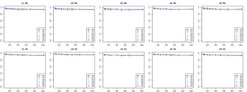
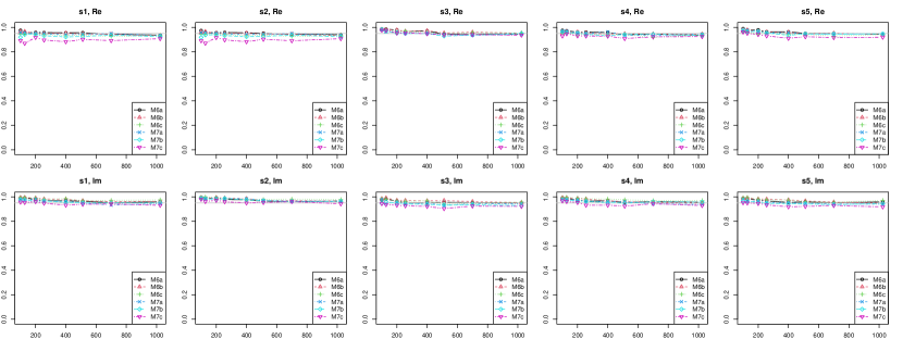
Figure 1: Uniform in $(\lambda,\tau_{1},\tau_{2})$ confidence bands, models M0-M7. Coverage probabilities with finite-population correction and weight functions $s_{1},\ldots,s_{5}$ as a function of $n$. Column $i$ corresponds to the weight function $s_{i}$, the first and third rows to the real parts, the second and fourth rows to the imaginary parts, of the integrated copula spectra.

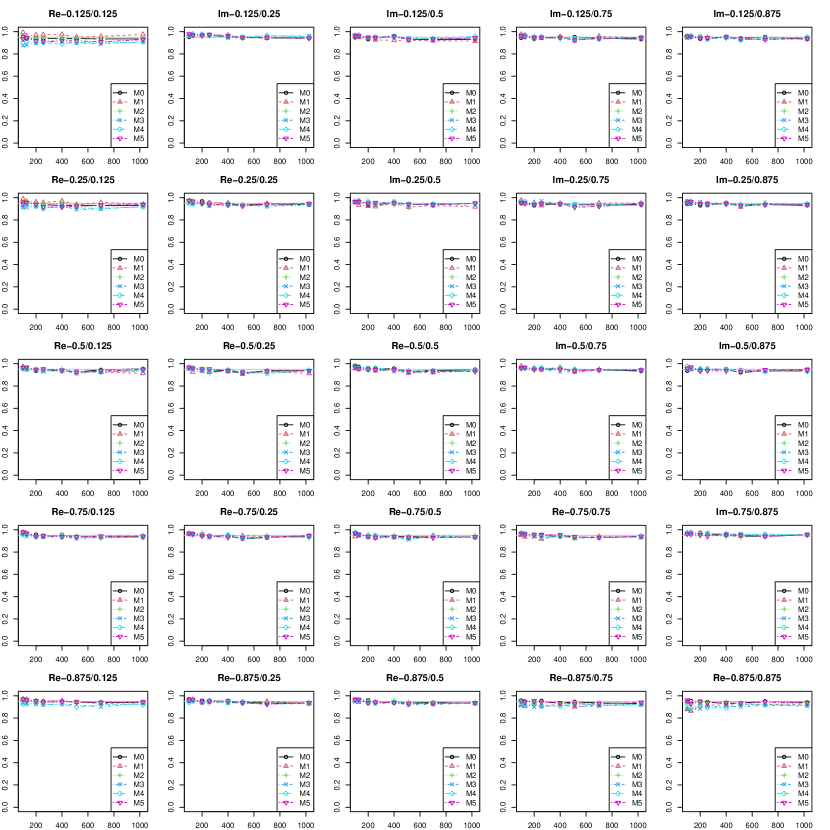
Figure 2: Uniform in $\lambda$ (pointwise in $(\tau_{1},\tau_{2})$) confidence bands, models M0-M5. Coverage probabilities with finite-population correction. Each subplot has a label indicating whether it is dealing with the real or imaginary part of the integrated spectrum, and which quantile levels $(\tau_{1},\tau_{2})$ were considered: e.g., the subplot with label Re-0.25/0.125 is about the real part of the integrated spectrum with $\tau_{1}=0.25$ and $\tau_{2}=0.125$.

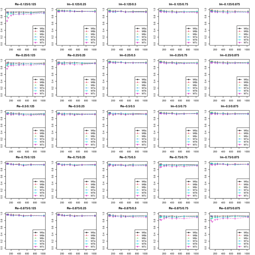
Figure 3: Uniform in $\lambda$ (pointwise in $(\tau_{1},\tau_{2})$) confidence bands, models M6-M7. Coverage probabilities with finite-population correction. Each subplot has a label indicating whether it is dealing with the real or imaginary part of the integrated spectrum, and which quantile levels $(\tau_{1},\tau_{2})$ were considered: e.g., the subplot with label Re-0.25/0.125 is about the real part of the integrated spectrum with $\tau_{1}=0.25$ and $\tau_{2}=0.125$.

5.1 Confidence bands

In this subsection, models M0-M7 from Table 1 are used to study the empirical coverage of the confidence bands described in Section 4.1. We consider $n\!\in~{}\!\!\{100,128,200,256,400,512,700,1024\}$ and, for each $n$ (choosing powers of 2 for $b$ allows for quick computation of the CR periodograms), $b\in B(n):=\{2^{4},2^{5},\ldots,\}\cap[0,n/2]$; as a rule of thumb, we selected

$$b^{\rm rt}_{n}:=\max\{2^{j}:2^{j}\leq 2n^{2/3},\ j=4,\ldots,8\},$$ (29)

yielding $b=32,32,64,64,64,128,128,128$ for $n=100,128,200,256,400,512,700,1024$, respectively. As for the Fourier frequencies in (15), we put $d=32$. Figure 1, Figure 2

We simulated $R=1000$ independent series for each configuration. For each of them, we computed the confidence band as explained in Section 4.1. To obtain their empirical coverage, we compare them with the actual value of the integrated copula spectral density. The latter can be computed precisely for M0; else, it was obtained from $500,000$ simulated CR periodograms.

The finite-population correction in (15) was applied; without it, the results (not shown here) are significantly worse: the correction, thus, is essential in numerical applications.

We throughout used $\alpha=0.05$. We simulated pointwise in $(\tau_{1},\tau_{2})$ coverage for all $\tau_{1},\tau_{2}$ in $\{1/16,\ldots,15/16\}$. For the uniform procedures, maxima with respect to all 15 quantile levels were used [see Appendix .4 for a detailed description of how coverage is computed]. For pointwise coverage, we only display results for $\tau_{1},\tau_{2}\in\{0.125,0.25,0.5,0.75,0.875\}$.

Figure 1 reports, for models M0-M7 and the $(\lambda,\tau_{1},\tau_{2})$-uniform procedure with finite-population correction (15), the coverage probabilities as functions of the sample size. For weighting, we have used the weights $s_{1},\ldots,s_{5}$ defined in the Appendix. All results are very close to the nominal 0.95 level; the equal weights function $s_{4}$ yields the best results. Figures 2 (for models M0-M5) and 3 (for models M6-M7) report the coverage probabilities of the $\lambda$-uniform, $(\tau_{1},\tau_{2})$-pointwise procedure, still with finite-population correction. Here and in subsequent tables reporting $(\tau_{1},\tau_{2})$-pointwise results, we have followed the convention to show the results for real parts on and below the diagonal and the results for imaginary parts above the diagonal. Overall, the method (with finite-population correction) works well. As expected, large sample sizes are required to obtain reasonable coverage probability for extreme quantiles, for example, $\tau_{1}=\tau_{2}=0.125,0.875$. Especially, the construction of confidence bands for extreme quantiles in models M3, M4, and M7c is challenging. For $\tau_{1}\neq\tau_{2}$, the results for imaginary parts are better than for real parts.

5.2 Time-reversibility

In this subsection, we evaluate, based on models M0-M7 and M8-M11, the finite-sample performance of the tests for time-reversibility introduced in Section 4.2 and compare it to that of their main competitors. The simulation procedure is essentially the same as in Section 5.1: for each value of the sample size $n$ in $\{100,128,150,200,256,400,512,700,1024\}$, a subsampling block size $b(n)$ is chosen via the rule of thumb (29). The maxima in the test statistic (22) are taken over the frequency range $\{2\pi\ell/32;\ell=0,1,\ldots,16\}$ and the quantiles $\{\tau_{1},\tau_{2}=k/8;k=1,\ldots,7\}$, with the weight functions $s_{1},\ldots,s_{5}$ defined in the Appendix. The significance level throughout is $\alpha=0.05$.

For each case, $R=1000$ replications were generated. For each replication, two tests were performed, based on $T_{\rm TR1}^{(n,b,t)}$ (no finite-population correction) and $T_{\rm TR1\_fpc}^{(n,b,t)}:=\frac{T_{\rm TR1}^{(n,b,t)}}{(1-b/n)^{1/2}}$ (finite-population correction), respectively. The resulting rejection frequencies with weight function $s_{4}\equiv 1$ (empirical sizes for M0, M2, M6, empirical powers for M1, M3, M4, M5, and M7) are shown in Figure 4 for $T_{\rm TR1}^{(n,b,t)}$ and Figure 5 for $T_{\rm TR1\_fpc}^{(n,b,t)}$, respectively.

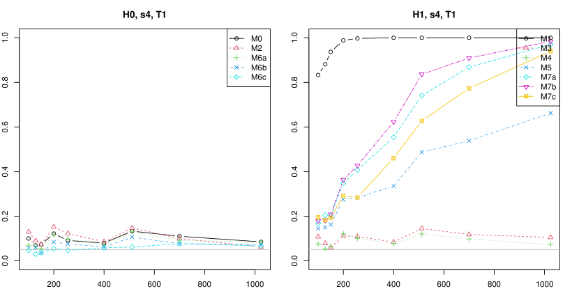
Figure 4: Empirical sizes (left, time-reversible models M0, M2, and M6a-c) and powers (right, time-irreversible models M1, M3, M4, M5, and M7a-c) as functions of $n$, of the tests for time-reversibility based on $T_{\rm TR1}^{(n,b,t)}$ (no finite-population correction).

The test based on $T_{\rm TR1}^{(n,b,t)}$ suffers of size distortion (over–rejection) while the size control, for the test based on $T_{\rm TR1\_fpc}^{(n,b,t)}$, is good. The finite-population correction, thus, is highly recommended. We can see that the power of our tests is high for large sample sizes except for M3-M5. Results for other weight functions are provided in the online supplement.

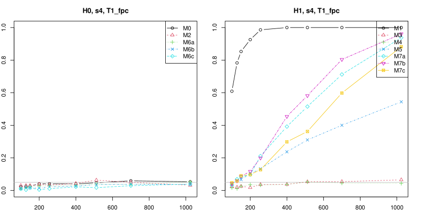
Figure 5: Empirical sizes (left, time-reversible models M0, M2, and M6a-c) and powers (right, time-irreversible models M1, M3, M4, M5, and M7a-c) as functions of $n$, of the tests for time-reversibility based on $T_{\rm TR1\_fpc}^{(n,b,t)}$ (with finite-population correction).

Next, we compare our tests with the few existing ones, namely, the tests proposed by Ramsey and Rothman, (1996), Chen et al., (2000), Paparoditis and Politis, (2002), and Beare and Seo, (2014), based on the test statistics

$$\begin{array}[]{rlrcl}T_{\rm RR}&:=\dfrac{1}{n-1}\sum_{t=0}^{n-2}(X_{t+1}^{2}X_{t}-X_{t+1}X_{t}^{2}),&T_{\rm CCK}&:=&\dfrac{1}{n-1}\sum_{t=0}^{n-2}\dfrac{X_{t+1}-X_{t}}{1+(X_{t+1}-X_{t})^{2}}\\ T_{\rm PP}&:=\dfrac{1}{n-1}\sum_{t=0}^{n-2}I\{X_{t+1}>X_{t}\}-\dfrac{1}{2},\ \text{and }&T_{\rm BS}&:=&\sup_{(x,y)\in\mathbb{R}^{2}}\left|\hat{F}_{n}(x,y)-\hat{F}_{n}(y,x)\right|,\end{array}$$ (30)

respectively, where $\hat{F}_{n}(x,y):=\sum_{t=0}^{n-2}I\{X_{t}\leq x,X_{t+1}\leq y\}/(n-1)$. The critical values of these tests are calculated via local bootstrap (see Sections 3.2 and 3.3 in Beare and Seo, (2014)). The intuition behind $T_{\rm CCK}$ and $T_{\rm PP}$ is that time-reversibility of the process $X_{t}$ implies the symmetry of $(X_{t}-X_{t-1})$ about the origin, while $T_{\rm RR}$ is motivated by the fact that ${\rm E}X_{t}^{2}X_{t-1}={\rm E}X_{t}X_{t-1}^{2}$ under time-reversibility if $X_{t}$ has finite third moments. These facts, however, are just necessary conditions for time-reversibility. As for $T_{\rm BS}$, it is based on a property of Markov processes, which are time-reversible at lag one if and only if the copula of $(X_{0},X_{1})$ is. Figure 6

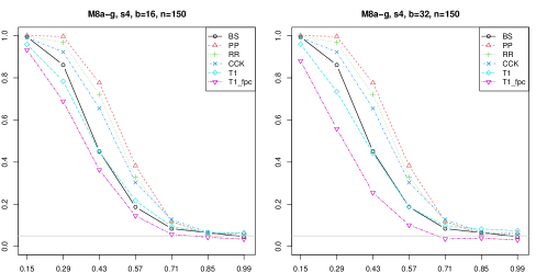
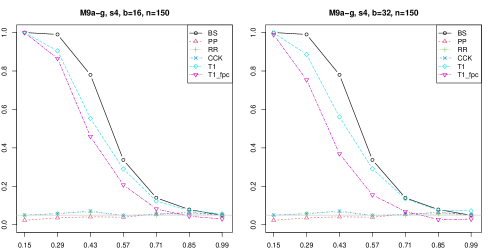
Figure 6: Empirical power of the tests for time-reversibility described in Section 4.2 for $n=150$. The upper and lower plots correspond to M8$a$–$g$ and M9$a$–$g$, the left and right ones to subsampling block sizes $b=16$ and $b=32$, respectively.

Our comparison is based on simulations of models M8-M9 with sample size $n=150$ (Figure 6), of models M10-M11 with sample size $n=512$ (Figure 7), with subsampling block sizes $b=16$ and $b=32$ and weight function $s_{4}\equiv 1$. Other settings and simulations have been performed, and yield similar results. Empirical power plots are provided in Figures 6 and 7, with increasing degree of time-reversibility (measured by the parameters $\lambda$ and $\gamma^{-1}$, respectively, with value one corresponding to the null hypothesis of time-reversibility) on the horizontal axis. Model M9 is such that, among the competitors (30), only $T_{\rm BS}$ can detect time-irreversibility; models M10 and M11 are such that none of these competitors can detect time-irreversibility. Our tests were implemented with and without finite population correction.

Figure 6 shows the expected result that the power of all tests increases with the degree of time-irreversibility for M8; the same holds true for M9, but only for our tests and the test based on $T_{\rm BS}$, while $T_{\rm PP}$, $T_{\rm RR}$, and $T_{\rm CCK}$ (which are best under M8) are totally powerless. Our tests behave quite well in all cases, although outperformed by the test based on $T_{\rm BS}$. Figure 7, however,

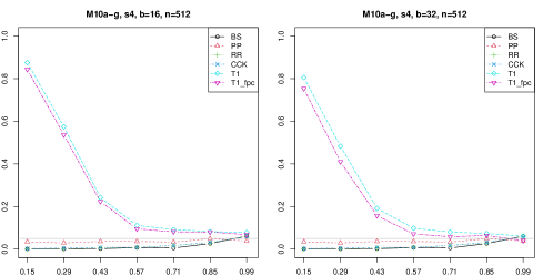
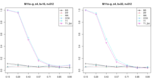
Figure 7: Empirical power of the tests for time-reversibility described in Section 4.2 for $n=512$. The upper plots and lower plots correspond to M10$a$–$g$ and M11$a$–$g$, the left and right ones to subsampling block sizes $b=16$ and $b=32$, respectively.

establishes that in models M10 and M11 with moderate degree of time-irreversibility, our tests very efficiently do reject time-reversibility while all their competitors, including the $T_{\rm BS}$-based one, fall short from detecting anything. The finite population correction and the choice of the subsampling block size apparently have little impact, irrespective of the model and the sample size. Additional simulations can be found in the online Supplement.

5.3 Asymmetry in tail dynamics

In order to study the empirical size and power of the test for quantile symmetry introduced in Section 4.3, we simulated observations from models M0–M7c and M12a–M15. For each sample size $n\in\{100,128,200,256,400,512,700,1024\}$, a subsampling block size $b(n)$ is chosen via the rule of thumb (29). As in Section 5.2, the maxima in statistic (27) were taken over the frequency range $\{2\pi\ell/32;\ell=0,1,\ldots,16\}$ and the quantiles $\{\tau_{1},\tau_{2}=k/16;k=2,3,4\}$, with weight functions $s_{4}\equiv 1$. Significance level throughout is $\alpha=0.05$. Figure 4

For each case, $R=1000$ replications were generated. For each replication, two tests were performed, based on the test statistics $T_{\rm EQ}^{(n,b,t)}$ (as defined in (27); no finite-population correction) and $T_{\rm EQ\_fpc}^{(n,b,t)}:=(1-b/n)^{-1/2}T_{\rm EQ}^{(n,b,t)}\vspace{1mm}$ (with finite-population correction), respectively.

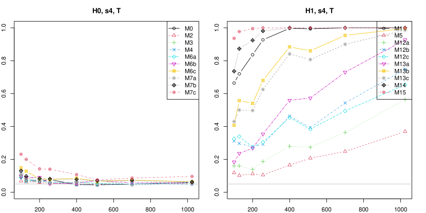
Figure 8: Empirical sizes (left) and powers (right), as functions of $n$, of the tests for tail symmetry based on $T_{\rm EQ}^{(n,b,t)}$ under various models.

The resulting rejection frequencies (empirical sizes for M0, M2, M3, M4, M6a-c, and M7a- c, empirical powers for M1, M5, M12a-c, M13a-c, M14, and M15) are displayed in Figure 8 for $T_{\rm EQ}^{(n,b,t)}$ and Figure 9 for $T_{\rm EQ\_fpc}$.

The test based on $T_{\rm EQ}^{(n,b,t)}\vspace{-.5mm}$ (Figure 8) exhibits significant size distortions for small sample sizes—particularly so under models M7b–c and M6c. The test based on the corrected statistic $\vspace{.7mm}T_{\rm EQ\_fpc}^{(n,b,t)}$ provides much better results in that respect, although overrejection is still present under M7b–c. The finite population correction, thus, is still recommended. As for empirical powers, they all increase with the sample size; detecting tail asymmetry in M5 and, to a lesser extent, in M12a remains difficult. Simulation results for additional weight functions are provided in the online Supplement.

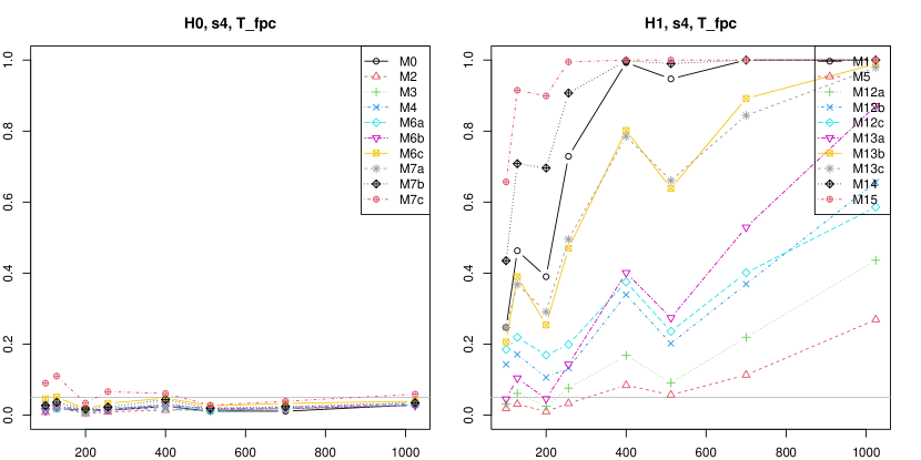
Figure 9: Empirical sizes (left) and powers (right), as functions of $n$, of the tests for tail symmetry based on $T_{\rm TR1\_fpc}$ described in Section 4.3 under various models. The models in the left plots and right plots belong to the null and alternative, respectively.

Additional details on simulations

.4 Computation of coverage frequencies

The coverage probability of the procedure that is uniform with respect to $\lambda$ and pointwise with respect to $(\tau_{1},\tau_{2})$ for a real part is defined by the empirical probability (with respect to the iterations) of the event, for fixed $\tau_{1}$ and $\tau_{2}$,

$$\Big{\{}\Re{\boldsymbol{\mathfrak{F}}}\phantom{F\!\!\!\!}\Big{(}\frac{2\pi\ell}{d},\tau_{1},\tau_{2}\Big{)}\in\widehat{I}_{\alpha,{\rm Re}}^{D}\Big{(}\frac{2\pi\ell}{d},\tau_{1},\tau_{2}\Big{)}\text{ for all $\ell=1,\ldots,d$}\Big{\}},$$

where $\Re{\boldsymbol{\mathfrak{F}}}$ is the true spectrum derived by the direct calculation for (M0) and the true spectrum simulated by quantspec for the other cases. In case of the simulated spectra, they are available at the Fourier frequencies $2\pi k/N$, with $N=2^{11}$ and we round down to the next available such frequency $2\pi\lfloor N\ell/x\rfloor/N$, where $\ell\in 0,\ldots,\lfloor d/2\rfloor$.

The coverage probability of the procedure that is uniform with respect to $(\lambda,\tau_{1},\tau_{2})$ for a real part is defined by the empirical probability (with respect to the iterations) of the event

$$\Big{\{}\Re{\boldsymbol{\mathfrak{F}}}\phantom{F\!\!\!\!}\Big{(}\frac{2\pi\ell}{d},\tau_{1},\tau_{2}\Big{)}\in\widehat{I}_{\alpha,{\rm Re}}^{E}\Big{(}\frac{2\pi\ell}{d},\tau_{1},\tau_{2}\Big{)}\text{ for all $\ell=1,\ldots,d$ and all $(\tau_{1},\tau_{2})$ in the range}\Big{\}}.$$

The coverage probabilities of the procedure that is uniform with respect to $\lambda$ and pointwise with respect to $(\tau_{1},\tau_{2})$ and of the procedure that is uniform with respect to $(\lambda,\tau_{1},\tau_{2})$ for imaginary parts are defined in the same way.

.5 Weight functions

The weight functions $s_{1}-s_{5}$ are defined as

$$s_{1}(\tau_{1},\tau_{2}):= \sqrt{\tau_{1}(1-\tau_{1})\tau_{2}(1-\tau_{2})},$$

$$s_{2}(\tau_{1},\tau_{2}):= \max\{\tau_{1},\tau_{2}\}-\tau_{1}\tau_{2},$$

$$s_{3}(\tau_{1},\tau_{2}):= \min\{\tau_{1},\tau_{2}\}-\tau_{1}\tau_{2},$$

$$s_{4}(\tau_{1},\tau_{2}):= 1,$$

$$s_{5}(\tau_{1},\tau_{2}):= \sqrt{s_{3}(\tau_{1},\tau_{2})}.$$

.6 Detailed definitions of the models used in simulations

Models M0–M15 are defined, for $j=a,b,c$ and $i=a,\ldots,g$, as

$$X_{t}\sim\mathcal{N}(0,1)\text{ i.\,i.\,d.},$$ (M0)

$$X_{t}=0.1\Phi^{-1}(U_{t})+1.9(U_{t}-0.5)X_{t-1},$$ (M1)

$$X_{t}=-0.36X_{t-2}+\varepsilon_{t},$$ (M2)

$$X_{t}=\bigl{(}1/1.9+0.9X_{t-1}^{2}\bigr{)}^{1/2}\varepsilon_{t},$$ (M3)

$$X_{t}=\sigma_{t}\varepsilon_{t},\textrm{ where }\sigma_{t}^{2}=0.01+0.4X_{t-1}^{2}+0.5\sigma_{t-1}^{2},$$ (M4)

$$X_{t}=\sigma_{t}\varepsilon_{t},~{}\ln(\sigma_{t}^{2})=0.1+0.21(|X_{t-1}|-\textnormal{\mbox{I\negthinspace E}}|X_{t-1}|)-0.2X_{t-1}+0.8\ln(\sigma_{t-1}^{2}),$$ (M5)

$$X_{t}=\phi_{j}X_{t-1}+\varepsilon_{t}, j$$ (M6)

$$X_{t}=\phi_{j}X_{t-1}+\nu_{t}, j$$ (M7)

$$X_{t}=C_{1}^{-1}(U_{t}|X_{t-1})\quad\text{with $\gamma_{i}$}, i$$ (M8)

$$X_{t}=C_{2}^{-1}(U_{t}|X_{t-1})\quad\text{with $\lambda_{i}$}, i$$ (M9)

$$X_{2t-1}=Y_{t},\ X_{2t}=Y_{t}^{\prime}\quad\text{with $Y_{t}$ and $Y_{t}^{\prime}\sim$ (M8$i$),\quad$Y_{t}\mathop{\perp\!\!\!\!\perp}Y_{t}^{\prime}$}, i$$ (M10)

$$X_{2t-1}=Y_{t},\ X_{2t}=Y_{t}^{\prime}\quad\text{with $Y_{t}$ and $Y_{t}^{\prime}\sim$ (M9$i$),\quad$Y_{t}\mathop{\perp\!\!\!\!\perp}Y_{t}^{\prime}$}, i$$ (M11)

$$X_{t}=C_{3}^{-1}(U_{t}|X_{t-1})\quad\text{with $\tau_{3j}$}, j$$ (M12)

$$X_{t}=C_{4}^{-1}(U_{t}|X_{t-1})\quad\text{with $\tau_{4j}$}, j$$ (M13)

$$X_{t}=C_{5}^{-1}(U_{t}|X_{t-1}),$$ (M14)

$$X_{t}=C_{6}^{-1}(U_{t}|X_{t-1}).$$ (M15)

In (M1), $(U_{t})$ denotes a sequence of i.i.d. standard uniform random variables, and $\Phi$ denotes the cdf of $\mathcal{N}(0,1)$. This model is from the class of QAR(1) processes, which was introduced by Koenker and Xiao, (2006). In (M2), $(\varepsilon_{t})$ denotes a sequence of standard normal white noise. This AR(2) process was previously considered by Li, (2012). (M3) is ARCH(1) process previously considered by Lee and Rao, (2012). (M4) and (M5) are GARCH(1,1) and EGARCH(1,1,1) models, respectively, previously considered by Birr et al., (2019). (M6$j$) is AR(1) model with a Gaussian innovation. The AR coefficient of this model is defined as $\phi_{j}:=0.3,0.5,0.7$ for $j=a,b,c$ in order. In (M7$j$), $(\nu_{t})$ denotes a sequence of i.i.d. standard Cauchy distribution. This is AR(1) model with a Cauchy innovation. The ordinary spectral density of (M7$j$) does not exist. In (M8$i$) and (M9$i$), $U_{t}$ denotes a sequence of i.i.d. standard uniform distribution. The conditional distribution function $C_{j}^{-1}(u|v)$ is defined, for $(U,V)$ whose joint distribution follows $C_{j}$, as $C_{j}^{-1}(u|v):={\rm P}(U\leq u|V=v)$ for $j=1,2$. The function $C_{1}(u,v)$ is the asymmetric Gumbel copula, which is defined as

$$C_{1}(u,v):=u^{1-\alpha}v^{1-\beta}\exp\left[-\left\{(-\alpha\log u)^{\gamma}+(-\beta\log v)^{\gamma}\right\}^{1/\gamma}\right],$$

where $(\alpha,\beta)=(1,0.5)$ and $\gamma\geq 1$. The function $C_{2}(u,v)$ is the zero total circulation copula, which is defined, for $\lambda\in[0,1]$, as

$$C_{2}(u,v):=\int_{0}^{u}\int_{0}^{v}\lambda+(1-\lambda)c_{0}(s,t){\rm d}s{\rm d}t,$$

where

$$c_{2}(u,v):=\begin{cases}1&\{0\leq v<1/4,1/4\leq u<1/2\}\cup\{1/4\leq v<1/2,3/4\leq u\leq 1\}\\ &\cup\{1/2\leq v<3/4,0\leq u<1/4\},\cup\{3/4\leq v\leq 1,1/2\leq u<3/4\}\\ 0&\text{otherwise},\end{cases}$$

and the generalized inverse $C_{j}^{-1}$ is calculated via a grid of 1000 points equispaced over $[0,1]$. Let $\gamma_{i}^{-1}$ and $\lambda_{i}$ take values $0.15,0.29,0.43,0.57,0.71,0.85,0.99$ for $i=a,\ldots,g$, respectively. These models were considered by Beare and Seo, (2014) in their simulation. When $\gamma_{i}=~{}\!1$ and $\lambda_{i}=1$, both models reduce to the product copula. Therefore, (M8$i$) with $\gamma_{i}=1$ and (M9$i$) with $\lambda_{i}=1$ are time-reversible. The models (M10$i$) and (M11$i$) are designed that any time-reversibility tests based on a first-order Markov process cannot detect time-irreversibility. In (M12$j$), the function $C_{3}(u,v)$ is the Gumbel copula, which is defined as

$$C_{3}(u,v):=\exp\left[-\left\{(-\log u)^{\gamma}+(-\log v)^{\gamma}\right\}^{1/\gamma}\right],$$

where $\gamma=1/(1-\tau_{3j})\geq 1$ with Kendall’s tau $\tau_{3j}$ for $C_{3}$. In (M13$j$), the function $C_{4}(u,v)$ is the Clayton copula, which is defined as

$$C_{4}(u,v):=(u^{-\gamma}+v^{-\gamma}-1)^{-1/\gamma},$$

where $\gamma=2\tau_{4j}/(1-\tau_{4j})>0$ with Kendall’s tau $\tau_{4j}$ for $C_{4}$. The parameters $\tau_{3j}$ and $\tau_{4j}$ are defined as $\tau_{3j},\tau_{4j}:=0.25,0.5,0.75$ for $j=a,b,c$, respectively. These models are considered by Li and Genton, (2013) in their simulation. In (M14), the function $C_{5}(u,v)$ is the copula 3 of Nelsen, (1993, Figure 1), which is defined as

$$C_{5}(u,v):=\int_{0}^{u}\int_{0}^{v}c_{5}(s,t){\rm d}s{\rm d}t,$$

where

$$c_{5}(u,v):=\begin{cases}1&\{0\leq v<1/4,0\leq u<1/4\}\cup\{0\leq v<1/4,3/4\leq u<1\}\\ &\cup\{1/4\leq v<1/2,1/2\leq u\leq 1\}\cup\{1/2\leq v<3/4,1/4\leq u\leq 3/4\}\\ &\cup\{3/4\leq v<1,0\leq u<1/2\},\\ 0&\text{otherwise}.\end{cases}$$

In (M15), the function $C_{6}(u,v)$ is the copula 6 of Nelsen, (1993, Figure 1), which is defined as

$$C_{6}(u,v):=\int_{0}^{u}\int_{0}^{v}c_{6}(s,t){\rm d}s{\rm d}t,$$

where

$$c_{6}(u,v):=\begin{cases}1&\{0\leq v<1/2,1/4\leq u<3/4\}\cup\{1/2\leq v\leq 1,0\leq u<1/4\}\\ &\cup\{1/2\leq v\leq 1,3/4\leq u\leq 1\},\\ 0&\text{otherwise}.\end{cases}$$

The models M12j–M15 are not radially symmetric.

[Acknowledgments] The first three authors contributed equally to the paper and are listed alphabetically. The authors are grateful to Brendan K. Beare and Juwon Seo for kindly sharing their Matlab codes for Section 5.2.

This work has been supported in part by the Collaborative Research Center “Statistical modeling of nonlinear dynamic processes” (SFB 823, Teilprojekt A1,C1) of the German Research Foundation (DFG). Yuichi Goto was supported by JSPS Grant-in-Aid for Research Activity Start-up under Grant Number JP21K20338. Stanislav Volgushev was partially supported by a discovery grant from NSERC of Canada,

Online Supplement

Appendix A Proofs

A.1 Proof of Lemma 3.1

Proof.

Throughout the proof, let $\Phi_{k}$ and $\Phi$ denote the cumulative distribution functions of

$$(X_{k},X_{0})^{T}\sim\mathcal{N}_{2}\Big{(}\Big{(}\begin{array}[]{c}0\\ 0\end{array}\Big{)},\Big{(}\begin{array}[]{cc}1&\rho_{k}\\ \rho_{k}&1\end{array}\Big{)}\Big{)}$$

and $X_{0}\sim\mathcal{N}\big{(}0,1\big{)}$, respectively.

Note that

$$\boldsymbol{\mathfrak{G}}(\lambda;\tau_{1},\tau_{2})={} \frac{1}{2\pi}\sum_{k\in{\mathbb{Z}}\backslash\{0\}}\gamma_{k}^{U}(\tau_{1},\tau_{2})\frac{i}{k}(e^{-ik\lambda}-1)$$

$$={} \frac{1}{2\pi}\sum_{k\in{\mathbb{Z}}\backslash\{0\}}\big{(}C_{k}(\tau_{1},\tau_{2})-\tau_{1}\tau_{2}\big{)}\frac{i}{k}(e^{-ik\lambda}-1).$$

Furthermore, as $(X_{t})_{t\in{\mathbb{Z}}}$ is Gaussian, by Sklar’s theorem [see Sklar, (1959)],

$$C_{k}(\tau_{1},\tau_{2}):=C\big{(}\tau_{1},\tau_{2},\rho(k)\big{)}=\Phi_{k}\big{(}\Phi^{-1}(\tau_{1}),\Phi^{-1}(\tau_{2})\big{)}.$$

We first provide a bound on $\gamma_{k}^{U}(\tau_{1},\tau_{2})-\tau_{1}\tau_{2}$. Observe the following representation:

$$\gamma_{k}^{U}(\tau_{1},\tau_{2})-\tau_{1}\tau_{2}=\Phi_{k}\big{(}\Phi^{-1}(\tau_{1}),\Phi^{-1}(\tau_{2})\big{)}-\tau_{1}\tau_{2}$$

$$=\int_{-\infty}^{\Phi^{-1}(u)}\int_{-\infty}^{\Phi^{-1}(v)}\frac{1}{2\pi\sqrt{1-\rho_{k}^{2}}}\exp\Big{(}-\frac{x^{2}-2\rho_{k}xy+y^{2}}{2(1-\rho_{k}^{2})}\Big{)}-\frac{1}{2\pi}\exp\Big{(}-\frac{x^{2}+y^{2}}{2}\Big{)}\mathrm{d}x\mathrm{d}y$$

$$=\int_{-\infty}^{\Phi^{-1}(u)}\int_{-\infty}^{\Phi^{-1}(v)}h(x,y,\rho_{k})-h(x,y,0)\mathrm{d}x\mathrm{d}y$$

where

$$h(x,y,\rho):=\frac{1}{2\pi\sqrt{1-\rho^{2}}}\exp\Big{(}-\frac{x^{2}-2\rho xy+y^{2}}{2(1-\rho^{2})}\Big{)}.$$

Now, from a Taylor expansion, we find

$$\Big{|}h(x,y,\rho)-h(x,y,0)\Big{|}\leq|\rho|\Big{|}\frac{\partial h(x,y,\rho)}{\partial\rho}\big{|}_{\rho=\kappa(x,y)}\Big{|}$$

where $\kappa(x,y)$ is a value between $0$ and $\rho$. In particular, $|\kappa(x,y)|\leq|\rho|$ for any $x,y$. A straightforward calculation shows that there exists a function $H:\mathbb{R}^{2}\to[0,\infty)$, independent of $\kappa(x,y)$ such that for all $\kappa(x,y)\in[-1/2,1/2]$

$$\Big{|}\frac{\partial h(x,y,\rho)}{\partial\rho}\big{|}_{\rho=\kappa(x,y)}\Big{|}\leq H(x,y)$$

for all $x,y\in R^{2}$ and such that

$$K:=\int_{\mathbb{R}}\int_{\mathbb{R}}H(x,y)\mathrm{d}x\mathrm{d}y<\infty.$$

Summarizing, we have shown that for any $\rho_{k}\in[-1/2,1/2]$ and any $\tau_{1},\tau_{2}\in(0,1)$

$$|\gamma_{k}^{U}(\tau_{1},\tau_{2})-\tau_{1}\tau_{2}|\leq K|\rho_{k}|.$$

Since by assumption $\sum_{k}|\rho_{k}|/|k|<\infty$, we can have $|\rho_{k}|>1/2$ for at most a finite set of $k$. Thus,

$$\frac{1}{2\pi}\sum_{k\in{\mathbb{Z}}\backslash\{0\}}|\gamma_{k}^{U}(\tau_{1},\tau_{2})\frac{i}{k}(e^{-ik\lambda}-1)|\leq\frac{1}{\pi}\sum_{k\in{\mathbb{Z}}\backslash\{0\}}|\gamma_{k}^{U}(\tau_{1},\tau_{2})|/|k|$$

$$\leq \sum_{k:|\rho_{k}|\geq 1/2}|\gamma_{k}^{U}(\tau_{1},\tau_{2})|+K\sum_{k:|\rho_{k}|<1/2}\frac{|\rho_{k}|}{|k|}<\infty.$$ (31)

Next note that, employing Leibniz’s integral rule, we have

$$\frac{\partial\big{(}C(u,v;\rho)-uv\big{)}}{\partial u}$$

$$={} \frac{\partial}{\partial u}\int_{-\infty}^{\Phi^{-1}(u)}\int_{-\infty}^{\Phi^{-1}(v)}\frac{1}{2\pi\sqrt{1-\rho^{2}}}\exp\Big{(}-\frac{x^{2}-2\rho xy+y^{2}}{2(1-\rho^{2})}\Big{)}\mathrm{d}x\mathrm{d}y-v$$

$$={} \frac{d\Phi^{-1}(u)}{du}\int_{-\infty}^{\Phi^{-1}(v)}\frac{1}{2\pi\sqrt{1-\rho^{2}}}\exp\Big{(}-\frac{y^{2}-2\rho\Phi^{-1}(u)y+(\Phi^{-1}(u))^{2}}{2(1-\rho^{2})}\Big{)}\mathrm{d}y-\Phi(\Phi^{-1}(v)).$$

Observe that

$$\frac{d\Phi^{-1}(u)}{du}=\frac{1}{\Phi^{\prime}(\Phi^{-1}(u))}=\frac{1}{\frac{1}{\sqrt{2\pi}}\exp\big{(}-\frac{(\Phi^{-1}(u))^{2}}{2}\big{)}}=\sqrt{2\pi}\exp\Big{(}\frac{(\Phi^{-1}(u))^{2}}{2}\Big{)}$$

and, by adding a square,

$$\exp\Big{(}-\frac{y^{2}-2\rho\Phi^{-1}(u)y+(\Phi^{-1}(u))^{2}}{2(1-\rho^{2})}\Big{)}={} \exp\Big{(}-\frac{[y-\rho\Phi^{-1}(u)]^{2}+(1-\rho^{2})(\Phi^{-1}(u))^{2}}{2(1-\rho^{2})}\Big{)}$$

$$={} \exp\Big{(}-\frac{[y-\rho\Phi^{-1}(u)]^{2}}{2(1-\rho^{2})}\Big{)}\exp\Big{(}-\frac{(\Phi^{-1}(u))^{2}}{2}\Big{)}.$$

Thus, altogether,

$$\frac{\partial\big{(}C(u,v;\rho)-uv\big{)}}{\partial u}={} \int_{-\infty}^{\Phi^{-1}(v)}\frac{1}{\sqrt{2\pi(1-\rho^{2})}}\exp\Big{(}-\frac{[y-\rho\Phi^{-1}(u)]^{2}}{2(1-\rho^{2})}\Big{)}\mathrm{d}y-\Phi(\Phi^{-1}(v))$$

$$={} \Phi\Big{(}\frac{\Phi^{-1}(v)-\rho\Phi^{-1}(u)}{\sqrt{1-\rho^{2}}}\Big{)}-\Phi\big{(}\Phi^{-1}(v)\big{)}.$$

Next, let $g(u,v;\rho):=\frac{\Phi^{-1}(v)-\Phi^{-1}(u)\rho}{\sqrt{1-\rho^{2}}}$ and observe that $g(u,v;0)=\Phi^{-1}(v)$. The function $\rho\mapsto\Phi(g(u,v;\rho))$ is continuous and differentiable on $(-1,1)$. Thus, by the mean value theorem, for any $\rho\in[-1+\varepsilon,1-\varepsilon]$ with $0<\varepsilon<1$ there exists $\rho_{0}$ with $|\rho_{0}|\leq|\rho|$ such that

$$\Phi\big{(}g(u,v;\rho)\big{)}-\Phi\big{(}g(u,v;0)\big{)}=\frac{\partial\Phi\big{(}g(u,v;\rho)\big{)}}{\partial\rho}\Big{|}_{\rho=\rho_{0}}\cdot\rho.$$

Since

$$\frac{\partial\Phi\big{(}g(u,v;\rho)\big{)}}{\partial\rho}\Big{|}_{\rho=\rho_{0}}=\frac{\partial g(u,v;\rho)}{\partial\rho}\Big{|}_{\rho=\rho_{0}}\frac{d\Phi(x)}{dx}\Big{|}_{x=g(u,v,\rho_{0})}$$

$$={} \frac{-\Phi^{-1}(u)\sqrt{1-\rho_{0}^{2}}+\big{(}\Phi^{-1}(v)-\rho_{0}\Phi^{-1}(u)\big{)}\rho_{0}(1-\rho_{0}^{2})^{-1/2}}{1-\rho_{0}^{2}}\frac{1}{\sqrt{2\pi}}e^{-g^{2}(u,v;\rho_{0})/2}$$

and, hence,

$$\sup_{u,v\in[\eta,1-\eta],\rho_{0}\in[-1+\varepsilon,1-\varepsilon]}\Big{|}\frac{\partial\Phi\big{(}g(u,v;\rho)\big{)}}{\partial\rho}\Big{|}_{\rho=\rho_{0}}\leq{} C_{\eta},$$

we obtain

$$\Big{|}\Phi\big{(}g(u,v;\rho)\big{)}-\Phi\big{(}g(u,v;0)\big{)}\Big{|}\leq{} |\rho|\Big{|}\frac{\partial\Phi\big{(}g(u,v;\rho)\big{)}}{\partial\rho}\Big{|}_{\rho=\rho_{0}}\leq C_{\eta}\cdot|\rho|.$$

Therefore,

$$\frac{1}{2\pi}\sum_{k\in{\mathbb{Z}}\backslash\{0\}} \sup_{\tau_{1},\tau_{2}\in[\eta,1-\eta]}\Big{|}\frac{\partial\big{(}C(u,v;\rho(k))-uv\big{)}}{\partial u}\Big{|}_{(u,v)=(\tau_{1},\tau_{2})}\big{|}\frac{i}{k}(e^{ik\lambda}-1)\big{|}$$

$$\leq{} \frac{1}{2\pi}\sum_{k\in{\mathbb{Z}}\backslash\{0\}}\big{(}C_{\eta}|\rho(k)|\big{)}\frac{2}{|k|}<\infty,$$

where we have used that, by assumption, $\sum_{k\in{\mathbb{Z}}\backslash\{0\}}\frac{|\rho(k)|}{|k|}<\infty$. Combining this with (31) we can apply Theorem 7.17 in Rudin et al., (1964) to conclude that the partial derivatives

$$\frac{\partial\boldsymbol{\mathfrak{G}}(\lambda,u,v)}{\partial u}\Big{|}_{(u,v)=(\tau_{1},\tau_{2})}$$

exist and are continuous on $\{(\lambda;\tau_{1},\tau_{2})\in[0,\pi]\times[\eta,1-\eta]\times[\eta,1-\eta]\}$. ∎

A.2 Proof of Theorem 3.1

We begin by deriving an alternative representation for the copula-based spectral distribution function defined in (2) and introduce some additional notation.

Observe that from definitions (3) and (4) we can derive the following representation of the copula rank periodogram:

$$\mathcal{I}_{n,R}^{\tau_{1},\tau_{2}}\big{(}\frac{2\pi s}{n}\big{)}={} \frac{1}{2\pi n}d_{n,R}^{\tau_{1}}\big{(}\frac{2\pi s}{n}\big{)}d_{n,R}^{\tau_{2}}\big{(}-\frac{2\pi s}{n}\big{)}$$

$$={} \frac{1}{2\pi n}\sum_{t_{1}=0}^{n-1}I\{\hat{F}_{n}(X_{t_{1}})\leq\tau_{1}\}e^{-it_{1}\frac{2\pi s}{n}}\sum_{t_{2}=0}^{n-1}I\{\hat{F}_{n}(X_{t_{2}})\leq\tau_{2}\}e^{it_{2}\frac{2\pi s}{n}}.$$ (32)

Since $\sum_{t=0}^{n-1}e^{-it2\pi s/n}=0$ for $s\not\in n{\mathbb{Z}}$, we have, for $\tau\in[0,1]$,

$$\sum_{t=0}^{n-1}I\{\hat{F}_{n}(X_{t})\leq\tau\}e^{-it\frac{2\pi s}{n}}={} \sum_{t=0}^{n-1}\big{(}I\{\hat{F}_{n}(X_{t})\leq\tau\}-a\big{)}e^{-it\frac{2\pi s}{n}},$$ (33)

where $a\in\mathbb{R}$ can be chosen arbitrarily. Using property (33) in (A.2), after rearranging sums, we obtain

$$\mathcal{I}_{n,R}^{\tau_{1},\tau_{2}}\big{(}\frac{2\pi s}{n}\big{)}={} \frac{1}{2\pi n}\sum_{|k|\leq n-1}\sum_{t\in\mathcal{T}_{k}}\big{(}I\{\hat{F}_{n}(X_{t+k})\leq\tau_{1}\}-a\big{)}\big{(}I\{\hat{F}_{n}(X_{t})\leq\tau_{2}\}-b\big{)}e^{-ik\frac{2\pi s}{n}},$$ (34)

with arbitrary $a,b\in\mathbb{R}$,

$$\mathcal{T}_{k}:=\{t\in\{0,\dots,n-1\}|t,t+k\in\{0,\dots,n-1\}\}$$

and $k\in\{-(n-1),\dots,n-1\}$. Next, using (34) in the definition of the estimator of the spectral distribution function (2) and rearranging sums yields

$$\widehat{\boldsymbol{\mathfrak{F}}}\phantom{F\!\!\!\!\!}_{n,R}(\lambda;\tau_{1},\tau_{2})={} \frac{1}{2\pi}\sum_{|k|\leq n-1}\frac{2\pi}{n}\sum_{s=1}^{n-1}I\big{\{}0\leq\frac{2\pi s}{n}\leq\lambda\big{\}}e^{-ik\frac{2\pi s}{n}}\frac{n-|k|}{n}$$

$$\cdot\frac{1}{n-|k|}\sum_{t\in\mathcal{T}_{k}}\big{(}I\{\hat{F}_{n}(X_{t+k})\leq\tau_{1}\}-a\big{)}\big{(}I\{\hat{F}_{n}(X_{t})\leq\tau_{2}\}-b\big{)}.$$

Define the weights

$$w_{n,\lambda}(k):=\frac{2\pi}{n}\sum_{s=1}^{n-1}I\big{\{}0\leq\frac{2\pi s}{n}\leq\lambda\big{\}}e^{-ik\frac{2\pi s}{n}}$$ (35)

and the rank-based copula cumulant function of order $k$

$$\hat{\gamma}_{k}^{R}(\tau_{1},\tau_{2})={} \frac{1}{n-|k|}\sum_{t\in\mathcal{T}_{k}}\Big{(}I\{\hat{F}_{n}(X_{t+k})\leq\tau_{1}\}-a\Big{)}\Big{(}I\{\hat{F}_{n}(X_{t})\leq\tau_{2}\}-b\Big{)}.$$ (36)

Then, we obtain

$$\widehat{\boldsymbol{\mathfrak{F}}}\phantom{F\!\!\!\!\!}_{n,R}(\lambda;\tau_{1},\tau_{2}):={} \frac{1}{2\pi}\sum_{|k|\leq n-1}w_{n,\lambda}(k)\frac{n-|k|}{n}\hat{\gamma}_{k}^{R}(\tau_{1},\tau_{2})$$

$$={} \frac{1}{2\pi}\sum_{0<|k|\leq n-1}w_{n,\lambda}(k)\frac{n-|k|}{n}\hat{\gamma}_{k}^{R}(\tau_{1},\tau_{2})+\frac{1}{2\pi}w_{n,\lambda}(0)\hat{\gamma}_{0}^{R}(\tau_{1},\tau_{2})$$ (37)

as an alternative representation of the estimator of the copula spectral distribution function. Similarly, the copula spectral distribution function has the alternative representation

$$\boldsymbol{\mathfrak{F}}(\lambda;\tau_{1},\tau_{2})={} \frac{1}{2\pi}\sum_{k\in{\mathbb{Z}}\backslash\{0\}}\gamma_{k}^{U}(\tau_{1},\tau_{2})\frac{i}{k}(e^{-ik\lambda}-1)+\frac{\lambda}{2\pi}(\tau_{1}\wedge\tau_{2}-\tau_{1}\tau_{2}).$$

In the subsequent analysis, we sometimes will consider versions of $\widehat{\boldsymbol{\mathfrak{F}}}\phantom{F\!\!\!\!\!}_{n,R}(\lambda;\tau_{1},\tau_{2})$ and $\boldsymbol{\mathfrak{F}}(\lambda;\tau_{1},\tau_{2})$, where the terms corresponding to lag $0$ are removed, that is,

$$\hat{\boldsymbol{\mathfrak{G}}}_{n,R}(\lambda;\tau_{1},\tau_{2}):=\frac{1}{2\pi}\sum_{0<|k|\leq n-1}\frac{2\pi}{n}\sum_{s=1}^{n-1}I\big{\{}0\leq\frac{2\pi s}{n}\leq\lambda\big{\}}e^{-ik\frac{2\pi s}{n}}\frac{n-|k|}{n}\hat{\gamma}_{k}^{R}(\tau_{1},\tau_{2})$$

and $\boldsymbol{\mathfrak{G}}(\lambda;\tau_{1},\tau_{2})$ as defined in (7). Also, in the analysis of the asymptotic properties, instead of the process

$$\{\widehat{\boldsymbol{\mathfrak{F}}}\phantom{F\!\!\!\!\!}_{n,R}(\lambda;\tau_{1},\tau_{2})\}_{(\lambda;\tau_{1},\tau_{2})\in[0,\pi]\times[0,1]^{2}},$$

we often prove intermediate results for the process

$$\{\widehat{\boldsymbol{\mathfrak{F}}}\phantom{F\!\!\!\!\!}_{n,U}(\lambda;\tau_{1},\tau_{2})\}_{(\lambda;\tau_{1},\tau_{2})\in[0,\pi]\times[0,1]^{2}},$$

where $\widehat{\boldsymbol{\mathfrak{F}}}\phantom{F\!\!\!\!\!}_{n,U}(\lambda;\tau_{1},\tau_{2})$ is defined exactly as $\widehat{\boldsymbol{\mathfrak{F}}}\phantom{F\!\!\!\!\!}_{n,R}(\lambda;\tau_{1},\tau_{2})$ but with the actual distributions function $F$ replacing the empirical one $\hat{F}_{n}$. More precisely, in order to prove the weak convergence of the process $\{\widehat{\boldsymbol{\mathfrak{F}}}\phantom{F\!\!\!\!\!}_{n,R}(\lambda;\tau_{1},\tau_{2})\}_{(\lambda;\tau_{1},\tau_{2})\in[0,\pi]\times[\eta,1-\eta]^{2}}$ for $0<\eta<1/2$, we derive, according to Lemma 2.2.2 in van der Vaart and Wellner, (1996), the stochastic equicontinuity for the process $\{\widehat{\boldsymbol{\mathfrak{F}}}\phantom{F\!\!\!\!\!}_{n,U}(\lambda;\tau_{1},\tau_{2})\}_{(\lambda;\tau_{1},\tau_{2})\in[0,\pi]\times[\eta,1-\eta]^{2}}$. The impact of replacing the true distribution functions $F$ by the empirical versions $\hat{F}_{n}$ in $\{\widehat{\boldsymbol{\mathfrak{F}}}\phantom{F\!\!\!\!\!}_{n,R}(\lambda;\tau_{1},\tau_{2})\}_{(\lambda;\tau_{1},\tau_{2})\in[0,\pi]\times[\eta,1-\eta]^{2}}$ is then seen in the derivation of the covariance structure of the limiting process.

We are now ready to start with the main proof. We first prove several intermediate results for the process

$$\mathbb{G}_{n,U}(\lambda;\tau_{1},\tau_{2}):=\sqrt{n}\Big{(}\widehat{\boldsymbol{\mathfrak{F}}}\phantom{F\!\!\!\!\!}_{n,U}(\lambda;\tau_{1},\tau_{2})-\boldsymbol{\mathfrak{F}}(\lambda;\tau_{1},\tau_{2})\Big{)}$$

indexed by $(\lambda;\tau_{1},\tau_{2})\in[0,\pi]\times[\eta,1-\eta]^{2}$, where

$$\widehat{\boldsymbol{\mathfrak{F}}}\phantom{F\!\!\!\!\!}_{n,U}(\lambda;\tau_{1},\tau_{2}):={} \frac{2\pi}{n}\sum_{s=1}^{n-1}I\big{\{}0\leq\frac{2\pi s}{n}\leq\lambda\big{\}}\mathcal{I}_{n,U}^{\tau_{1},\tau_{2}}\big{(}\frac{2\pi s}{n}\big{)},$$

with $U_{t}:=F(X_{t})$ and

$$\mathcal{I}_{n,U}^{\tau_{1},\tau_{2}}\left(\omega\right)=(2\pi n)^{-1}d_{n,U}^{\tau_{1}}(\omega)d_{n,U}^{\tau_{2}}(-\omega),\qquad d_{n,U}^{\tau}(\omega):=\sum_{t=0}^{n-1}I\{U_{t}\leq\tau\}e^{-i\omega t}.$$

As for $\widehat{\boldsymbol{\mathfrak{F}}}\phantom{F\!\!\!\!\!}_{n,R}(\lambda;\tau_{1},\tau_{2})$, we have

$$\widehat{\boldsymbol{\mathfrak{F}}}\phantom{F\!\!\!\!\!}_{n,U}(\lambda;\tau_{1},\tau_{2})={} \frac{1}{2\pi}\sum_{0<|k|\leq n-1}w_{n,\lambda}(k)\frac{n-|k|}{n}\hat{\gamma}_{k}^{U}(\tau_{1},\tau_{2})+\frac{1}{2\pi}w_{n,\lambda}(0)\hat{\gamma}_{0}^{U}(\tau_{1},\tau_{2}),$$

where $w_{n,\lambda}(k)$ is defined in (35),

$$\hat{\gamma}_{k}^{U}(\tau_{1},\tau_{2})={} \frac{1}{n-|k|}\sum_{t\in\mathcal{T}_{k}}\Big{(}I\{U_{t+k}\leq\tau_{1}\}-a\Big{)}\Big{(}I\{U_{t}\leq\tau_{2}\}-b\Big{)}$$ (38)

with $\mathcal{T}_{k}:=\{t\in\{0,\dots,n-1\}|t,t+k\in\{0,\dots,n-1\}\}$, $k\in\{-(n-1),\dots,n-1\}$, where $a,b\in\mathbb{R}$ can be chosen arbitrarily since $\sum_{t=0}^{n-1}e^{-it2\pi s/n}=0$ for $s\not\in n{\mathbb{Z}}$.

Finally, as for the rank-based versions, we define

$$\hat{\boldsymbol{\mathfrak{G}}}_{n,U}(\lambda;\tau_{1},\tau_{2}):=\frac{1}{2\pi}\sum_{0<|k|\leq n-1}\frac{2\pi}{n}\sum_{s=1}^{n-1}I\big{\{}0\leq\frac{2\pi s}{n}\leq\lambda\big{\}}e^{-ik\frac{2\pi s}{n}}\frac{n-|k|}{n}\hat{\gamma}_{k}^{U}(\tau_{1},\tau_{2})$$

and

$$\boldsymbol{\mathfrak{G}}(\lambda;\tau_{1},\tau_{2}):=\frac{1}{2\pi}\sum_{k\in{\mathbb{Z}}\backslash\{0\}}\gamma_{k}^{U}(\tau_{1},\tau_{2})\frac{i}{k}(e^{-ik\lambda}-1),$$

where the terms corresponding to lag $k=0$ have been removed.

A.2.1 Proof of Theorem 3.1 – Main arguments

The proof of Theorem 3.1 is rather technical and consists of a series of lemmas and intermediate results. To facilitate the reading we give an overview of the most important arguments of the proof.

For all $n\in\mathbb{N}$, consider the stochastic process

$$\mathbb{G}_{n,R}(\lambda;\tau_{1},\tau_{2}):=\sqrt{n}\Big{(}\widehat{\boldsymbol{\mathfrak{F}}}\phantom{F\!\!\!\!\!}_{n,R}(\lambda;\tau_{1},\tau_{2})-\boldsymbol{\mathfrak{F}}(\lambda;\tau_{1},\tau_{2})\Big{)}$$ (39)

indexed by $(\lambda;\tau_{1},\tau_{2})\in[0,\pi]\times[\eta,1-\eta]^{2}$. Observe that since $F$ is assumed to be continuous, the ranks of $X_{0},\dots,X_{n-1}$ are almost surely the same as the ranks of $U_{0},\dots,U_{n-1}$, i.e., without loss of generality, we can assume the marginals to be uniformly distributed. In what follows, let $\hat{F}_{n,U}$ denote the empirical distribution function of $U_{0},\dots,U_{n-1}$. With $\hat{\tau}:=\hat{F}_{n,U}^{-1}(\tau)$, we have, by Lemma B.1 (the proof of which is deferred to Section B.3),

$$\widehat{\boldsymbol{\mathfrak{F}}}\phantom{F\!\!\!\!\!}_{n,R}(\lambda;\tau_{1},\tau_{2})=\widehat{\boldsymbol{\mathfrak{F}}}\phantom{F\!\!\!\!\!}_{n,U}(\lambda,\hat{\tau}_{1},\hat{\tau}_{2})+o_{\mathbb{P}}(n^{-1/2}).$$ (40)

Furthermore, by Lemma B.2 (which is also proved in Section B.3),

$$\mathbb{G}_{n,R}(\lambda;\tau_{1},\tau_{2})={} \sqrt{n}\Big{(}\hat{\boldsymbol{\mathfrak{G}}}_{n,R}(\lambda;\tau_{1},\tau_{2})-\boldsymbol{\mathfrak{G}}(\lambda;\tau_{1},\tau_{2})\Big{)}+o_{\mathbb{P}}(1),$$

$$\mathbb{G}_{n,U}(\lambda;\tau_{1},\tau_{2})={} \sqrt{n}\Big{(}\hat{\boldsymbol{\mathfrak{G}}}_{n,U}(\lambda;\tau_{1},\tau_{2})-\boldsymbol{\mathfrak{G}}(\lambda;\tau_{1},\tau_{2})\Big{)}+o_{\mathbb{P}}(1),$$

and, therefore, we have the decomposition

$$\mathbb{G}_{n,R}(\lambda;\tau_{1},\tau_{2})={} \mathbb{G}_{n,U}(\lambda,\hat{\tau}_{1},\hat{\tau}_{2})-\mathbb{G}_{n,U}(\lambda;\tau_{1},\tau_{2})$$

$$+\mathbb{G}_{n,U}(\lambda;\tau_{1},\tau_{2})+\sqrt{n}\Big{(}\boldsymbol{\mathfrak{G}}(\lambda,\hat{\tau}_{1},\hat{\tau}_{2})-\boldsymbol{\mathfrak{G}}(\lambda;\tau_{1},\tau_{2})\Big{)}+o_{\mathbb{P}}(1)$$

$$={} \mathbb{G}_{n,U}(\lambda,\hat{\tau}_{1},\hat{\tau}_{2})-\mathbb{G}_{n,U}(\lambda;\tau_{1},\tau_{2})+\mathbb{G}_{n,U}(\lambda;\tau_{1},\tau_{2})$$

$$+\sqrt{n}\Big{(}(\hat{\tau}_{1}-\tau_{1})\frac{\partial\boldsymbol{\mathfrak{G}}}{\partial\tau_{1}}(\lambda;\tau_{1},\tau_{2})+(\hat{\tau}_{2}-\tau_{2})\frac{\partial\boldsymbol{\mathfrak{G}}}{\partial\tau_{2}}(\lambda;\tau_{1},\tau_{2})\Big{)}$$

$$+o_{\mathbb{P}}(1)$$ (41)

where, by Assumption (D),

$$\sqrt{n}\Big{(}\boldsymbol{\mathfrak{G}}(\lambda,\hat{\tau}_{1},\hat{\tau}_{2})-\boldsymbol{\mathfrak{G}}(\lambda;\tau_{1},\tau_{2})\Big{)}={}\sqrt{n}\sum_{j=1}^{2}(\hat{\tau}_{j}-\tau_{j})\frac{\partial\boldsymbol{\mathfrak{G}}}{\partial\tau_{j}}(\lambda;\tau_{1},\tau_{2})+o_{\mathbb{P}}(1),$$

as , by Lemma A.5 in Kley et al., 2016a ,

$$\sup_{\tau\in[0,1]}|\hat{F}_{n,U}^{-1}(\tau)-\tau|=O_{\mathbb{P}}(n^{-1/2}).$$

Moreover, noting that $\sqrt{n}\big{(}\hat{F}_{n,U}(\tau)-\tau\big{)}$ converges to a tight Gaussian limit with continuous sample paths [see the proof of Lemma A.5 in Kley et al., 2016b ], we obtain under the given assumptions by Vervaat’s Lemma [see Vervaat, (1972)],

$$\hat{\tau}_{j}-\tau_{j}=-\Big{(}\hat{F}_{n,U}(\tau_{j})-\tau_{j}\Big{)}+o_{\mathbb{P}}(n^{-1/2}).$$ (42)

Substituting (42) into (A.2.1) yields the decomposition

$$\mathbb{G}_{n,R}(\lambda;\tau_{1},\tau_{2})={} \mathbb{G}_{n,U}(\lambda,\hat{\tau}_{1},\hat{\tau}_{2})-\mathbb{G}_{n,U}(\lambda;\tau_{1},\tau_{2})+\mathbb{G}_{n,U}(\lambda;\tau_{1},\tau_{2})$$

$$+\sqrt{n}\sum_{j=1}^{2}(\tau_{j}-\hat{F}_{n,U}(\tau_{j}))G_{j}(\lambda;\tau_{1},\tau_{2})+o_{\mathbb{P}}(1),$$ (43)

where $G_{j}(\lambda;\tau_{1},\tau_{2}):=\frac{\partial\boldsymbol{\mathfrak{G}}}{\partial\tau_{j}}(\lambda;\tau_{1},\tau_{2});\,j=1,2$.

As a second step, to prove the weak convergence of $\mathbb{G}_{n,R}$, it suffices, by Lemmas 1.5.4 and 1.5.7 in van der Vaart and Wellner, (1996), to show that the finite-dimensional distributions converge in distribution and to prove stochastic equicontinuity. That is, we need to establish

• the convergence of the finite-dimensional distributions of the process (8), i.e.

  $$\Big{(}\mathbb{G}_{n,R}(\lambda_{j},\tau_{1}^{(j)},\tau_{2}^{(j)})\Big{)}_{j=1,\dots,L}\overset{\mathcal{D}}{\longrightarrow}\Big{(}\mathbb{G}(\lambda_{j},\tau_{1}^{(j)},\tau_{2}^{(j)})\Big{)}_{j=1,\dots,L}$$ (44)

  for any $(\lambda_{j},\tau_{1}^{(j)},\tau_{2}^{(j)})\in[0,\pi]\times[\eta,1-\eta]^{2},\,j=1,\dots,L$ and $L\in\mathbb{N}$ and

• stochastic equicontinuity, i.e., for all $x>0$,

  $$\lim_{\delta\downarrow 0}\limsup_{n\rightarrow\infty}\mathbb{P}\Big{(}\sup_{\begin{subarray}{c}(\lambda;\tau_{1},\tau_{2}),(\lambda^{\prime},\tau_{1}^{\prime},\tau_{2}^{\prime})\in[0,\pi]\times[\eta,1-\eta]^{2}\\ \|(\lambda;\tau_{1},\tau_{2})-(\lambda^{\prime},\tau_{1}^{\prime},\tau_{2}^{\prime})\|_{1}\leq\delta\end{subarray}}|\mathbb{G}_{n,R}(\lambda;\tau_{1},\tau_{2})-\mathbb{G}_{n,R}(\lambda^{\prime},\tau_{1}^{\prime},\tau_{2}^{\prime})|>x\Big{)}=0.$$ (45)

We start by proving the stochastic equicontinuity (45). In regard of equation (A.2.1), our proof consists of three steps:

• establish the stochastic equicontinuity of $\big{(}\mathbb{G}_{n,U}(\lambda;\tau_{1},\tau_{2})\big{)}_{(\lambda;\tau_{1},\tau_{2})\in[0,\pi]\times[\eta,1-\eta]^{2}}$;

• establish the stochastic equicontinuity of $\sqrt{n}(\hat{F}_{n,U}(\tau)-\tau)_{\tau\in[0,1]}$;

• show that

  $$\sup_{(\lambda;\tau_{1},\tau_{2})\in[0,\pi]\times[\eta,1-\eta]^{2}}\big{|}\mathbb{G}_{n,U}(\lambda,\hat{\tau}_{1},\hat{\tau}_{2})-\mathbb{G}_{n,U}(\lambda;\tau_{1},\tau_{2})\big{|}=o_{\mathbb{P}}(1).$$ (46)

The assertion in the second step has been established in Kley et al., 2016a and the third step follows from the first one (see Section B.1.1). For simplicity of notation, introduce $a:=(\lambda;\tau_{1},\tau_{2})$ and $b:=(\lambda^{\prime},\tau_{1}^{\prime},\tau_{2}^{\prime})\in[0,\pi]\times[\eta,1-\eta]^{2}$. The main part in the proof of the stochastic equicontinuity of $\mathbb{G}_{n,U}(\lambda;\tau_{1},\tau_{2})$ is the establishment of a uniform bound on the increments of the process $\mathbb{G}_{n,U}$. The derivation of this bound relies on two intermediate bounds. First, we need a general bound on the moments of $\mathbb{G}_{n,U}(a)-\mathbb{G}_{n,U}(b)$ which is obtained in Lemma B.4. Second, we provide in Lemma B.5 a sharper bound on the same increments when $a$ and $b$ are “close.”

We now turn to the proof of the weak convergence of the finite-dimensional distributions (44). From (46), we have

$$\mathbb{G}_{n,R}(\lambda;\tau_{1},\tau_{2})={} \mathbb{G}_{n,U}(\lambda;\tau_{1},\tau_{2})+\sqrt{n}\sum_{j=1}^{2}(\tau_{j}-\hat{F}_{n,U}(\tau_{j}))G_{j}(\lambda;\tau_{1},\tau_{2})+o_{\mathbb{P}}(1)$$

and hence, it suffices to show the convergence of the finite-dimensional distributions of the process

$$\mathbb{K}_{n}(\lambda;\tau_{1},\tau_{2}):=\mathbb{G}_{n,U}(\lambda;\tau_{1},\tau_{2})+\sqrt{n}\sum_{j=1}^{2}(\tau_{j}-\hat{F}_{n,U}(\tau_{j}))G_{j}(\lambda;\tau_{1},\tau_{2})$$

indexed by $(\lambda;\tau_{1},\tau_{2})\in[0,\pi]\times[\eta,1-\eta]^{2}$. By Lemma P4.5 of Brillinger, (1975), it suffices to prove that for any $\lambda_{1},\dots,\lambda_{J}\in[0,\pi]$, $J\in\mathbb{N}$ and any $\tau_{1}^{(1)},\dots,\tau_{1}^{(J)},\tau_{2}^{(1)},\dots,\tau_{2}^{(J)}\in[\eta,1-\eta]$, the cumulants of the vector

$$\Big{(}\mathbb{K}_{n}(\lambda_{1},\tau_{1}^{(1)},\tau_{2}^{(1)}),\overline{\mathbb{K}_{n}(\lambda_{1},\tau_{1}^{(1)},\tau_{2}^{(1)})},\dots,\mathbb{K}_{n}(\lambda_{L},\tau_{1}^{(J)},\tau_{2}^{(J)}),\overline{\mathbb{K}_{n}(\lambda_{J},\tau_{1}^{(J)},\tau_{2}^{(J)})}\Big{)}$$

converge to the corresponding cumulants of the vector

$$\Big{(}\mathbb{G}(\lambda_{1},\tau_{1}^{(1)}\tau_{2}^{(1)}),\overline{\mathbb{G}(\lambda_{1},\tau_{1}^{(1)}\tau_{2}^{(1)})},\dots,\mathbb{G}(\lambda_{J},\tau_{1}^{(J)}\tau_{2}^{(J)}),\overline{\mathbb{G}(\lambda_{J},\tau_{1}^{(J)}\tau_{2}^{(J)})}\Big{)}.$$

To this end, we proceed again in three steps:

• show that the first-order moments of $\mathbb{K}_{n}(\lambda_{1};\tau_{1},\tau_{2})$ vanish;

• show that the second-order moments yield the asymptotic covariance structure (3.1);

• show that the moments of order greater than two vanish.

The first assertion is proved in Lemma B.3; detailed proofs of the second and third ones can be found in Section B.2.

In the remaining part of this section, we present the proofs of (44) and (45), where technical details are deferred to Section B.

A.2.2 Proof of (45) – stochastic equicontinuity

Assertion (46) mainly follows by the stochastic equicontinuity of $\big{(}\mathbb{G}_{n,U}(\lambda;\tau_{1},\tau_{2})\big{)}_{(\lambda;\tau_{1},\tau_{2})\in[0,\pi]\times[\eta,1-\eta]^{2}}$ which will be proved in the rest of this section. Details of the proof of (46) can be found in Section B.1.1.

We now prove the stochastic equicontinuity of $\big{(}\mathbb{G}_{n,U}(\lambda;\tau_{1},\tau_{2})\big{)}_{(\lambda;\tau_{1},\tau_{2})\in[0,\pi]\times[\eta,1-\eta]^{2}}$. By Lemma B.3, it suffices to consider the process

$$\Big{(}\overline{\mathbb{G}}_{n,U}(\lambda;\tau_{1},\tau_{2})\Big{)}_{(\lambda;\tau_{1},\tau_{2})\in[0,\pi]\times[\eta,1-\eta]^{2}}:={} \Big{(}\sqrt{n}(\widehat{\boldsymbol{\mathfrak{F}}}\phantom{F\!\!\!\!\!}_{n,U}(\lambda;\tau_{1},\tau_{2})$$

$$\hskip 39.83368pt-\textnormal{\mbox{I\negthinspace E}}[\widehat{\boldsymbol{\mathfrak{F}}}\phantom{F\!\!\!\!\!}_{n,U}(\lambda;\tau_{1},\tau_{2})])\Big{)}_{(\lambda;\tau_{1},\tau_{2})\in[0,\pi]\times[\eta,1-\eta]^{2}}$$ (47)

and we need to prove that ,for all $x>0$,

$$\lim_{\delta\downarrow 0}\limsup_{n\rightarrow\infty}\mathbb{P}\Big{(}\sup_{\begin{subarray}{c}(\lambda;\tau_{1},\tau_{2}),(\lambda^{\prime},\tau_{1}^{\prime},\tau_{2}^{\prime})\in[0,\pi]\times[\eta,1-\eta]^{2}\\ \|(\lambda;\tau_{1},\tau_{2})-(\lambda^{\prime},\tau_{1}^{\prime},\tau_{2}^{\prime})\|_{1}\leq\delta\end{subarray}}|\overline{\mathbb{G}}_{n,U}(\lambda;\tau_{1},\tau_{2})-\overline{\mathbb{G}}_{n,U}(\lambda^{\prime},\tau_{1}^{\prime},\tau_{2}^{\prime})|>x\Big{)}=0.$$

This will be achieved by applying Lemma A.1 from Kley et al., 2016a to the process (A.2.2). Therefore, we will prove in Section B.1.2 that the assumptions for that lemma are fulfilled with the metric

$$d\big{(}(\lambda;\tau_{1},\tau_{2}),(\lambda^{\prime},\tau_{1}^{\prime},\tau_{2}^{\prime})\big{)}:=\|(\lambda;\tau_{1},\tau_{2})-(\lambda^{\prime},\tau_{1}^{\prime},\tau_{2}^{\prime})\|_{1}^{\gamma/2}$$

for a $\gamma>0$ that will be specified in the proof of (48). More precisely, for all $(\lambda;\tau_{1},\tau_{2}),(\lambda^{\prime},\tau_{1}^{\prime},\tau_{2}^{\prime})$ in $[0,\pi]\times[\eta,1-\eta]^{2}$ with $d\big{(}(\lambda;\tau_{1},\tau_{2}),(\lambda^{\prime},\tau_{1}^{\prime},\tau_{2}^{\prime})\big{)}\geq\bar{\eta}/2\geq 0$, we have

$$\|\overline{\mathbb{G}}_{n,U}(\lambda;\tau_{1},\tau_{2})-\overline{\mathbb{G}}_{n,U}(\lambda^{\prime},\tau_{1}^{\prime},\tau_{2}^{\prime})\|_{\Psi}\leq{} Kd\big{(}(\lambda;\tau_{1},\tau_{2}),(\lambda^{\prime},\tau_{1}^{\prime},\tau_{2}^{\prime})\big{)}$$ (48)

where $\Psi$ denotes the Orlicz norm $\|X\|_{\Psi}:=\inf\{C>0:\textnormal{\mbox{I\negthinspace E}}[\Psi(|X|/C)]\leq 1\}$.

In particular, (48) holds for $\Psi(x):=x^{8}$, i.e.  $L=4$. Denoting by $D(\varepsilon,d)$ the packing number of $T:=([0,\pi]\times[\eta,1-\eta]^{2},d)$ [cf. van der Vaart and Wellner, (1996), page 98], we have $D(\varepsilon,d)\asymp\varepsilon^{-6/\gamma}$. Therefore, by Lemma A.1 in Kley et al., 2016a , for all $x,\delta>0$ and all $\tilde{\eta}\geq\bar{\eta}_{n}$, there exists a random variable $S_{1}$ and a constant $K<\infty$ such that, for $s:=(\lambda;\tau_{1},\tau_{2})$ and $t:=(\lambda^{\prime},\tau_{1}^{\prime},\tau_{2}^{\prime})$,

$$\sup_{d(s,t)\leq\delta}|\overline{\mathbb{G}}_{n,U}(s)-\overline{\mathbb{G}}_{n,U}(t)|\leq{} S_{1}+2\sup_{d(s,t)\leq\bar{\eta}_{n},t\in\tilde{T}}|\overline{\mathbb{G}}_{n,U}(s)-\overline{\mathbb{G}}_{n,U}(t)|$$

with

$$\|S_{1}\|_{\Psi}\leq K\Big{[}\int_{\bar{\eta}_{n}/2}^{\tilde{\eta}}\Psi^{-1}\Big{(}D(\varepsilon,d)\Big{)}\mathrm{d}\varepsilon+(\delta+2\bar{\eta}_{n})\Psi^{-1}\Big{(}D^{2}(\tilde{\eta},d)\Big{)}\Big{]}$$

where the set $\tilde{T}$ contains at most $D(\bar{\eta}_{n},d)$ points. In particular, by Markov’s inequality [cf. van der Vaart and Wellner, (1996), page 96],

$$\mathbb{P}(|S_{1}|>x)\leq\Big{(}\Psi\Big{(}x[8K\Big{(}\int_{\bar{\eta}_{n}/2}^{\tilde{\eta}}\Psi^{-1}\Big{(}D(\varepsilon,d)\Big{)}\mathrm{d}\varepsilon+(\delta+2\bar{\eta}_{n})\Psi^{-1}\Big{(}D^{2}(\tilde{\eta},d)\Big{)}\Big{)}\Big{]}^{-1}\Big{)}\Big{)}^{-1}.$$

Hence,

$$\mathbb{P}\Bigg{(}\sup_{\begin{subarray}{c}(\lambda;\tau_{1},\tau_{2}),(\lambda^{\prime},\tau_{1}^{\prime},\tau_{2}^{\prime})\in[0,\pi]\times[\eta,1-\eta]^{2}\\ \|(\lambda;\tau_{1},\tau_{2})-(\lambda^{\prime},\tau_{1}^{\prime},\tau_{2}^{\prime})\|_{1}\leq\delta^{2/\gamma}\end{subarray}}|\overline{\mathbb{G}}_{n,U}(\lambda;\tau_{1},\tau_{2})-\overline{\mathbb{G}}_{n,U}(\lambda^{\prime},\tau_{1}^{\prime},\tau_{2}^{\prime})|>x\Bigg{)}$$

$$={} \mathbb{P}\Bigg{(}\sup_{\begin{subarray}{c}(\lambda;\tau_{1},\tau_{2}),(\lambda^{\prime},\tau_{1}^{\prime},\tau_{2}^{\prime})\in[0,\pi]\times[\eta,1-\eta]^{2}\\ d((\lambda;\tau_{1},\tau_{2}),(\lambda^{\prime},\tau_{1}^{\prime},\tau_{2}^{\prime}))\leq\delta\end{subarray}}|\overline{\mathbb{G}}_{n,U}(\lambda;\tau_{1},\tau_{2})-\overline{\mathbb{G}}_{n,U}(\lambda^{\prime},\tau_{1}^{\prime},\tau_{2}^{\prime})|>x\Bigg{)}$$

$$\leq{} \mathbb{P}\Bigg{(}S_{1}+2\sup_{\begin{subarray}{c}(\lambda;\tau_{1},\tau_{2}),(\lambda^{\prime},\tau_{1}^{\prime},\tau_{2}^{\prime})\in[0,\pi]\times[\eta,1-\eta]^{2}\\ d((\lambda;\tau_{1},\tau_{2}),(\lambda^{\prime},\tau_{1}^{\prime},\tau_{2}^{\prime}))\leq\bar{\eta}_{n}\end{subarray}}|\overline{\mathbb{G}}_{n,U}(\lambda;\tau_{1},\tau_{2})-\overline{\mathbb{G}}_{n,U}(\lambda^{\prime},\tau_{1}^{\prime},\tau_{2}^{\prime})|>x\Bigg{)}$$

$$\leq{} \mathbb{P}(|S_{1}|>x/2)+\mathbb{P}\Bigg{(}\sup_{\begin{subarray}{c}(\lambda;\tau_{1},\tau_{2}),(\lambda^{\prime},\tau_{1}^{\prime},\tau_{2}^{\prime})\in[0,\pi]\times[\eta,1-\eta]^{2}\\ d((\lambda;\tau_{1},\tau_{2}),(\lambda^{\prime},\tau_{1}^{\prime},\tau_{2}^{\prime}))\leq\bar{\eta}_{n}\end{subarray}}|\overline{\mathbb{G}}_{n,U}(\lambda;\tau_{1},\tau_{2})-\overline{\mathbb{G}}_{n,U}(\lambda^{\prime},\tau_{1}^{\prime},\tau_{2}^{\prime})|>x/4\Bigg{)}$$

$$\leq{} \Big{(}\Big{(}\frac{x}{2}[8K\Big{(}\int_{\bar{\eta}_{n}/2}^{\tilde{\eta}}(C_{1}\varepsilon^{-6/\gamma})^{1/8}\mathrm{d}\varepsilon+(\delta+2\bar{\eta}_{n})(C_{2}\tilde{\eta}^{-12/\gamma})^{1/8}\Big{)}\Big{]}^{-1}\Big{)}^{8}\Big{)}^{-1}$$

$$+\mathbb{P}\Bigg{(}\sup_{\begin{subarray}{c}(\lambda;\tau_{1},\tau_{2}),(\lambda^{\prime},\tau_{1}^{\prime},\tau_{2}^{\prime})\in[0,\pi]\times[\eta,1-\eta]^{2}\\ d((\lambda;\tau_{1},\tau_{2}),(\lambda^{\prime},\tau_{1}^{\prime},\tau_{2}^{\prime}))\leq\bar{\eta}_{n}\end{subarray}}|\overline{\mathbb{G}}_{n,U}(\lambda;\tau_{1},\tau_{2})-\overline{\mathbb{G}}_{n,U}(\lambda^{\prime},\tau_{1}^{\prime},\tau_{2}^{\prime})|>x/4\Bigg{)}$$

$$\leq{} \Big{[}\frac{8\bar{K}}{x/2}\Big{(}\int_{\bar{\eta}_{n}/2}^{\tilde{\eta}}\varepsilon^{-3/(4\gamma)}\mathrm{d}\varepsilon+(\delta+2\bar{\eta}_{n})\tilde{\eta}^{-3/(2\gamma)}\Big{)}\Big{]}^{8}$$

$$+\mathbb{P}\Bigg{(}\sup_{\begin{subarray}{c}(\lambda;\tau_{1},\tau_{2}),(\lambda^{\prime},\tau_{1}^{\prime},\tau_{2}^{\prime})\in[0,\pi]\times[\eta,1-\eta]^{2}\\ d((\lambda;\tau_{1},\tau_{2}),(\lambda^{\prime},\tau_{1}^{\prime},\tau_{2}^{\prime}))\leq\bar{\eta}_{n}\end{subarray}}|\overline{\mathbb{G}}_{n,U}(\lambda;\tau_{1},\tau_{2})-\overline{\mathbb{G}}_{n,U}(\lambda^{\prime},\tau_{1}^{\prime},\tau_{2}^{\prime})|>x/4\Bigg{)}.$$

Now choose $1>\gamma>3/4$. Letting $n$ tend to infinity, the second term equals

$$\mathbb{P}\Bigg{(}\sup_{\begin{subarray}{c}(\lambda;\tau_{1},\tau_{2}),(\lambda^{\prime},\tau_{1}^{\prime},\tau_{2}^{\prime})\in[0,\pi]\times[\eta,1-\eta]^{2}\\ \|(\lambda;\tau_{1},\tau_{2})-(\lambda^{\prime},\tau_{1}^{\prime},\tau_{2}^{\prime})\|_{1}\leq 2^{2/\gamma}n^{-1/\gamma}\end{subarray}}|\overline{\mathbb{G}}_{n,U}(\lambda;\tau_{1},\tau_{2})-\overline{\mathbb{G}}_{n,U}(\lambda^{\prime},\tau_{1}^{\prime},\tau_{2}^{\prime})|>x/4\Bigg{)}$$

and converges to $0$ by Lemma B.5. Hence,

$$\lim_{\delta\downarrow 0}\limsup_{n\rightarrow\infty}\mathbb{P}\Bigg{(}\sup_{\begin{subarray}{c}(\lambda;\tau_{1},\tau_{2}),(\lambda^{\prime},\tau_{1}^{\prime},\tau_{2}^{\prime})\in[0,\pi]\times[\eta,1-\eta]^{2}\\ \|(\lambda;\tau_{1},\tau_{2})-(\lambda^{\prime},\tau_{1}^{\prime},\tau_{2}^{\prime})\|_{1}\leq\delta^{2/\gamma}\end{subarray}}|\overline{\mathbb{G}}_{n,U}(\lambda;\tau_{1},\tau_{2})-\overline{\mathbb{G}}_{n,U}(\lambda^{\prime},\tau_{1}^{\prime},\tau_{2}^{\prime})|>x\Bigg{)}$$

$$\leq{} \lim_{\delta\downarrow 0}\Big{[}\frac{8\bar{K}}{x}\Big{(}\int_{0}^{\tilde{\eta}}\varepsilon^{-3/(4\gamma)}\mathrm{d}\varepsilon+\delta\tilde{\eta}^{-3/(2\gamma)}\Big{)}\Big{]}^{8}$$

$$\leq{} \Big{[}\frac{8\bar{K}}{x}\int_{0}^{\tilde{\eta}}\varepsilon^{-3/(4\gamma)}\mathrm{d}\varepsilon\Big{]}^{8}$$

for every $x,\tilde{\eta}>0$. Since, $\tilde{\eta}$ can be chosen arbitrarily small, the integral can be made arbitrarily small and (45) follows.

A.2.3 Proof of (44) – convergence of the finite-dimensional distributions

In view of (A.2.1) and (46), it suffices to prove that the finite-dimensional distributions of

$$\mathbb{K}_{n}(\lambda;\tau_{1},\tau_{2}):=\mathbb{G}_{n,U}(\lambda;\tau_{1},\tau_{2})+\sqrt{n}\sum_{j=1}^{2}(\tau_{j}-\hat{F}_{n,U}(\tau_{j}))G_{j}(\lambda;\tau_{1},\tau_{2})$$

converge, i.e.  that

$$\Big{(}\mathbb{K}_{n}(\lambda_{j},\tau_{1}^{(j)},\tau_{2}^{(j)})\Big{)}_{j=1,\dots,J}\overset{\mathcal{D}}{\longrightarrow}\Big{(}\mathbb{G}(\lambda_{j},\tau_{1}^{(j)},\tau_{2}^{(j)})\Big{)}_{j=1,\dots,J}.$$

for any $(\lambda_{j},\tau_{1}^{(j)},\tau_{2}^{(j)})\in[0,\pi]\times[\eta,1-\eta]^{2},\,j=1,\dots,J$ and $J\in\mathbb{N}$, where the process $\mathbb{G}$ is defined in Theorem 3.1. For this purpose, we apply Lemma P4.5 of Brillinger, (1975), that is we prove that for any $\lambda_{1},\dots,\lambda_{J}\in[0,\pi]$, $J\in\mathbb{N}$ and any $\tau_{1}^{(1)},\dots,\tau_{1}^{(J)},\tau_{2}^{(1)},\dots,\tau_{2}^{(J)}$ in $[\eta,1-\eta]$, the cumulants of the vector

$$\Big{(}\mathbb{K}_{n}(\lambda_{1},\tau_{1}^{(1)},\tau_{2}^{(1)}),\overline{\mathbb{K}_{n}(\lambda_{1},\tau_{1}^{(1)},\tau_{2}^{(1)})},\dots,\mathbb{K}_{n}(\lambda_{J},\tau_{1}^{(J)},\tau_{2}^{(J)}),\overline{\mathbb{K}_{n}(\lambda_{J},\tau_{1}^{(J)},\tau_{2}^{(J)})}\Big{)}$$

converge to the corresponding cumulants of the vector

$$\Big{(}\mathbb{G}(\lambda_{1},\tau_{1}^{(1)}\tau_{2}^{(1)}),\overline{\mathbb{G}(\lambda_{1},\tau_{1}^{(1)}\tau_{2}^{(1)})},\dots,\mathbb{G}(\lambda_{J},\tau_{1}^{(J)}\tau_{2}^{(J)}),\overline{\mathbb{G}(\lambda_{J},\tau_{1}^{(J)}\tau_{2}^{(J)})}\Big{)}.$$

It can easily be shown that $\overline{\mathbb{K}_{n}(\lambda_{j},\tau_{1}^{(j)},\tau_{2}^{(j)})}=\mathbb{K}_{n}(\lambda_{j},\tau_{2}^{(j)},\tau_{1}^{(j)})$. Hence, it is equivalent to show the convergence of the cumulants of the vector

$$\Big{(}\mathbb{K}_{n}(\lambda_{1},\tau_{1}^{(1)},\tau_{2}^{(1)}),\mathbb{K}_{n}(\lambda_{1},\tau_{2}^{(1)},\tau_{1}^{(1)}),\dots,\mathbb{K}_{n}(\lambda_{J},\tau_{1}^{(J)},\tau_{2}^{(J)}),\mathbb{K}_{n}(\lambda_{J},\tau_{2}^{(J)},\tau_{1}^{(J)})\Big{)}.$$

It follows from Lemma B.3 that the first-order cumulants vanish as

$$|\textnormal{\mbox{I\negthinspace E}}[\mathbb{K}_{n}(\lambda;\tau_{1},\tau_{2})]|={} |\textnormal{\mbox{I\negthinspace E}}[\mathbb{G}_{n,U}(\lambda;\tau_{1},\tau_{2})+\sqrt{n}\sum_{j=1}^{2}(\tau_{j}-\hat{F}_{n,U}(\tau_{j}))G_{j}(\lambda;\tau_{1},\tau_{2})]|$$

$$={} \sqrt{n}|\textnormal{\mbox{I\negthinspace E}}[\widehat{\boldsymbol{\mathfrak{F}}}\phantom{F\!\!\!\!\!}_{n,U}(\lambda;\tau_{1},\tau_{2})]-\boldsymbol{\mathfrak{F}}(\lambda;\tau_{1},\tau_{2})|$$

$$={} O(n^{-1/2})$$

for any $\lambda\in[0,\pi]$ and $\tau_{1},\tau_{2}\in[\eta,1-\eta]$. Furthermore, for the second-order cumulants we obtain

$$\text{\rm cum}\Big{(} \mathbb{K}_{n}(\lambda;\tau_{1},\tau_{2}),\mathbb{K}_{n}(\mu,\xi_{1},\xi_{2})\Big{)}={}2\pi\int_{0}^{\lambda}\int_{0}^{\mu}\boldsymbol{\mathfrak{f}}\big{(}\alpha,-\alpha,\beta;\tau_{1},\tau_{2},\xi_{1},\xi_{2}\big{)}\mathrm{d}\alpha\mathrm{d}\beta$$

$$+2\pi\int_{0}^{\lambda\wedge\mu}\boldsymbol{\mathfrak{f}}\big{(}\alpha;\tau_{1},\xi_{2}\big{)}\boldsymbol{\mathfrak{f}}\big{(}-\alpha;\tau_{2},\xi_{1}\big{)}\mathrm{d}\alpha$$

$$\qquad-\sum_{j=1}^{2}G_{j}(\mu,\xi_{1},\xi_{2})2\pi\int_{0}^{\lambda}\boldsymbol{\mathfrak{f}}\big{(}\alpha,-\alpha;\tau_{1},\tau_{2},\xi_{j}\big{)}d\alpha$$

$$\qquad\qquad-\sum_{j=1}^{2}G_{j}(\lambda;\tau_{1},\tau_{2})2\pi\int_{0}^{\lambda}\boldsymbol{\mathfrak{f}}\big{(}\alpha,-\alpha;\xi_{1},\xi_{2},\tau_{j}\big{)}d\alpha$$

$$\qquad\qquad\qquad+\sum_{j_{1}=1}^{2}\sum_{j_{2}=1}^{2}G_{j_{1}}(\lambda;\tau_{1},\tau_{2})G_{j_{2}}(\mu,\xi_{1},\xi_{2})2\pi\boldsymbol{\mathfrak{f}}\big{(}0;\tau_{j},\xi_{j}\big{)}+O(n^{-1}).$$ (49)

The details of the derivation of (A.2.3) are given in Section B.2.1.

It remains to show that all cumulants of order $2<l\leq 2J$ vanish. For this purpose we prove in Section B.2.2 that

$$\Big{|}\text{\rm cum}\Big{(}\mathbb{K}_{n}(\lambda_{1},\tau_{1}^{(1)},\tau_{2}^{(1)}),\dots,\mathbb{K}_{n}(\lambda_{l},\tau_{1}^{(l)},\tau_{2}^{(l)})\Big{)}\Big{|}={}O(n^{-l/2+1}),$$ (50)

i.e. all cumulants of order greater than $2$ tend to zero. This proves that the limiting process $\mathbb{G}$ is Gaussian and concludes the proof of (44). $\Box$

A.3 Proof of Theorem 4.1

We only prove the second part; the proof of the first part indeed is similar but simpler, and we only focus on confidence bands for the real part of $\boldsymbol{\mathfrak{F}}$. Define

$$\tilde{S}_{n}:=\Big{\{}\frac{2\pi\ell}{d},\ell=0,1,\ldots,\lfloor d/2\rfloor\Big{\}}\times S_{n},\quad\tilde{S}:=[0,\pi]\times S.$$

Observe that

$$\mathds{P}\Big{(}\Re\boldsymbol{\mathfrak{F}}(\lambda;\tau_{1},\tau_{2})\in\Big{[}\Re\widehat{\boldsymbol{\mathfrak{F}}}\phantom{F\!\!\!\!\!}_{n,R}(\lambda;\tau_{1},\tau_{2})-C_{E,\alpha}s(\tau_{1},\tau_{2}),$$

$$\hskip 99.58464pt\Re\widehat{\boldsymbol{\mathfrak{F}}}\phantom{F\!\!\!\!\!}_{n,R}(\lambda;\tau_{1},\tau_{2})+C_{E,\alpha}s(\tau_{1},\tau_{2})\Big{]},\quad\forall(\lambda,\tau_{1},\tau_{2})\in\tilde{S}_{n}\Big{)}$$

$$=\mathds{P}\Big{(}\sup_{(\lambda,\tau_{1},\tau_{2})\in\tilde{S}_{n}}\frac{|\Re\widehat{\boldsymbol{\mathfrak{F}}}\phantom{F\!\!\!\!\!}_{n,R}(\lambda;\tau_{1},\tau_{2})-\Re\boldsymbol{\mathfrak{F}}(\lambda;\tau_{1},\tau_{2})|}{s(\tau_{1},\tau_{2})}\leq C_{E,\alpha}\Big{)}$$

$$=\mathds{P}\big{(}Y_{n}\leq G_{n}^{-1}(1-\alpha)\big{)},$$ (51)

where

$$Y_{n} :=\sqrt{n}\sup_{(\lambda,\tau_{1},\tau_{2})\in\tilde{S}_{n}}\frac{|\Re\widehat{\boldsymbol{\mathfrak{F}}}\phantom{F\!\!\!\!\!}_{n,R}(\lambda;\tau_{1},\tau_{2})-\Re\boldsymbol{\mathfrak{F}}(\lambda;\tau_{1},\tau_{2})|}{s(\tau_{1},\tau_{2})},$$ (52)

$$G_{n}(x) :=\frac{1}{n-b+1}\sum_{t=1}^{n-b+1}I\{\sqrt{b}\tilde{E}_{n,b,t}\leq x\},$$

$$G_{n}^{-1}(1-\alpha) :=\inf\{x:G_{n}(x)\geq 1-\alpha\},\quad\alpha\in(0,1).$$

By Corollary 1.3 and Remark 4.1 in Gaenssler et al., (2007), the distribution function $G$ of the random variable

$$Y:=\sup_{(\lambda,\tau_{1},\tau_{2})\in\tilde{S}}\frac{|\Re\mathbb{G}(\lambda,\tau_{1},\tau_{2})|}{s(\tau_{1},\tau_{2})}=\sup_{(\lambda,\tau_{1},\tau_{2})\in\tilde{S}}\max\Big{\{}\frac{-\Re\mathbb{G}(\lambda,\tau_{1},\tau_{2})}{s(\tau_{1},\tau_{2})},\frac{\Re\mathbb{G}(\lambda,\tau_{1},\tau_{2})}{s(\tau_{1},\tau_{2})}\Big{\}}$$

is continuous and strictly increasing on $(0,\infty)$. Let us show that $Y_{n}$ converges in distribution to $Y$. Defining

$$\widehat{Y}_{n}:=\sqrt{n}\sup_{(\lambda,\tau_{1},\tau_{2})\in\tilde{S}}\frac{|\Re\widehat{\boldsymbol{\mathfrak{F}}}\phantom{F\!\!\!\!\!}_{n,R}(\lambda;\tau_{1},\tau_{2})-\Re\boldsymbol{\mathfrak{F}}(\lambda;\tau_{1},\tau_{2})|}{s(\tau_{1},\tau_{2})},$$

note that $\widehat{Y}_{n}$ converges in distribution to $Y$ by Theorem 3.1 and the continuity of the map

$$f\mapsto\sup_{(\lambda,\tau_{1},\tau_{2})\in S}|f(\lambda;\tau_{1},\tau_{2})/s(\tau_{1},\tau_{2})|.$$

By Slutzky, it suffices to show that $\widehat{Y}_{n}-Y_{n}=o_{P}(1)$. Note that, for any bounded function $f$ on $\tilde{S}$ and any $\tilde{S}_{n}\subset S$, we have, by the triangle inequality,

$$\sup_{x\in\tilde{S}}|f(x)| \leq\sup_{x\in\tilde{S}}\inf_{y\in S_{n}}\Big{(}|f(x)-f(y)|+|f(y)|\Big{)}$$

$$\leq\sup_{x\in\tilde{S}}\inf_{y\in\tilde{S}_{n}}|f(x)-f(y)|+\sup_{z\in\tilde{S}_{n}}|f(z)|$$

which yields

$$0\leq\sup_{x\in\tilde{S}}|f(x)|-\sup_{x\in\tilde{S}_{n}}|f(x)|\leq\sup_{x\in\tilde{S}}\inf_{y\in\tilde{S}_{n}}|f(x)-f(y)|\leq\sup_{x,y\in S:\|x-y\|\leq d(\tilde{S}_{n},\tilde{S})}|f(x)-f(y)|.$$

Define

$$g_{n}(\lambda,\tau_{1},\tau_{2}):=\sqrt{n}\frac{|\Re\widehat{\boldsymbol{\mathfrak{F}}}\phantom{F\!\!\!\!\!}_{n,R}(\lambda;\tau_{1},\tau_{2})-\Re\boldsymbol{\mathfrak{F}}(\lambda;\tau_{1},\tau_{2})|}{s(\tau_{1},\tau_{2})}$$

and apply the above inequality with $x=(\lambda,\tau_{1},\tau_{2})$ and $f(x)=g_{n}(\lambda,\tau_{1},\tau_{2})$ to obtain

$$0\leq\widehat{Y}_{n}-Y_{n}\leq\sup_{x,y\in\tilde{S}:\|x-y\|\leq d(\tilde{S}_{n},\tilde{S})}|g_{n}(x)-g_{n}(y)|.$$

By a simple calculation and Theorem 3.1, the paths of $g_{n}$ are uniformly asymptotically equicontinuous, whence the right-hand side of the last display is $o_{P}(1)$. Indeed, for any fixed $\delta>0$ and $\varepsilon>0$, we have

$$\limsup_{n\to\infty}P\Big{(}\sup_{x,y\in S:\|x-y\|\leq d(\tilde{S}_{n},\tilde{S})}|g_{n}(x)-g_{n}(y)|\geq\varepsilon\Big{)}\leq\limsup_{n\to\infty}P\Big{(}\sup_{x,y\in\tilde{S}:\|x-y\|\leq\delta}|g_{n}(x)-g_{n}(y)|\geq\varepsilon\Big{)}.$$

Since the left-hand side above does not depend on $\delta$ we can take the limit $\lim_{\delta\downarrow 0}$ on both sides to obtain

$$\lim_{\delta\downarrow 0}\limsup_{n\to\infty}P\Big{(}\sup_{x,y\in\tilde{S}:\|x-y\|\leq d(\tilde{S}_{n},\tilde{S})}|g_{n}(x)-g_{n}(y)|\geq\varepsilon\Big{)}\\ \leq\lim_{\delta\downarrow 0}\limsup_{n\to\infty}P\Big{(}\sup_{x,y\in\tilde{S}:\|x-y\|\leq\delta}|g_{n}(x)-g_{n}(y)|\geq\varepsilon\Big{)}=0$$

where the last equality follows from uniform asymptotic equicontinuity. Since $\varepsilon>0$ was arbitrary this implies $\sup_{x,y\in\tilde{S}:\|x-y\|\leq\delta}|g_{n}(x)-g_{n}(y)|=o_{P}(1)\vspace{1mm}$. Thus, by continuity of the distribution of $Y$, we have, for all $x\in\mathbb{R}$,

$$\mathds{P}(Y_{n}\leq x)\rightarrow\mathds{P}(Y\leq x)=G(x).$$ (53)

Denote by $\rho_{L}$ the bounded Lipschitz metric on the space of distribution functions on $\mathbb{R}$: the following result will be established later in the proof

$$\rho_{L}(G_{n},G)\xrightarrow{\mathds{P}^{*}}0.$$ (54)

From (54) and the continuity of $G$, we obtain the following two convergences (note that both suprema are measurable since their value does not change if $\sup_{x\in\mathbb{R}}$ is replaced by $\sup_{x\in\mathbb{Q}}$ and the latter is taken over a countable set):

$$\sup_{x\in\mathbb{R}}|G_{n}(x)-G(x)|\xrightarrow{\mathds{P}}0,$$ (55)

and

$$\sup_{x\in\mathbb{R}}|G_{n}(x)-G_{n}(x-)|\xrightarrow{\mathds{P}}0.$$ (56)

Here (56) follows from (55) by continuity of $G$. Indeed, any continuous distribution function is also uniformly continuous, and we have, for any $\varepsilon>0$,

$$\sup_{x}|G_{n}(x)-G_{n}(x-)| \leq\sup_{x}|G_{n}(x)-G_{n}(x-\varepsilon)|$$

$$\leq 2\sup_{x}|G_{n}(x)-G(x)|+\sup_{x}|G(x)-G(x-\varepsilon)|.$$

Letting $\varepsilon\downarrow 0$, we obtain, from the uniform continuity of $G$,

$$\sup_{x}|G_{n}(x)-G_{n}(x-)|\leq 2\sup_{x}|G_{n}(x)-G(x)|.$$

To establish (55), note that, by Problem 23.1 in Van der Vaart, (2000), (55) is equivalent to $G_{n}(x)=G(x)+o_{\mathds{P}}(1)$ for every $x$, which can be established by a standard approximation of indicator functions through Lipschitz continuous functions.

Then, the assertion of the theorem follows from (51), (53), the continuity of $G$, (55), and (56). The coverage probability in (51) indeed is bounded from above by

$$\begin{split}\mathds{P}\big{(}G_{n}(Y_{n})\leq G_{n}\big{(}G_{n}^{-1}(1-\alpha)\big{)}\big{)}&=\mathds{P}\big{(}G(Y_{n})+r_{1,n}+r_{2,n}\leq 1-\alpha\big{)},\\ &\rightarrow\mathds{P}\big{(}G(Y)\leq 1-\alpha\big{)}=1-\alpha,\end{split}$$ (57)

where the first equality follows from the fact that $G_{n}$ is monotone increasing; for the second equality, letting $r_{1,n}:=G_{n}(Y_{n})-G(Y_{n})$ and $r_{2,n}:=1-\alpha-G_{n}\big{(}G_{n}^{-1}(1-\alpha)\big{)}$, note that $r_{1,n}=o_{\mathds{P}}(1)$ and $r_{2,n}=o_{\mathds{P}}(1)$ since

$$|r_{1,n}|=|G_{n}(Y_{n})-G(Y_{n})|\leq\sup_{x\in\mathbb{R}}|G_{n}(x)-G(x)|\xrightarrow{\mathds{P}}0$$

and, in view of Lemma 21.1 (ii), (iii) in Van der Vaart, (2000),

$$|r_{2,n}|=|1-\alpha-G_{n}\big{(}G_{n}^{-1}(1-\alpha)\big{)}|\leq\sup_{x\in\mathbb{R}}|G_{n}(x)-G_{n}(x-)|\xrightarrow{\mathds{P}}0.$$

Finally, as $G$ is continuous, it follows from the Continuous Mapping Theorem and Slutzky’s lemma, that

$$G(Y_{n})+o_{\mathds{P}}(1)\xrightarrow{\mathcal{D}}G(Y);$$

this completes the proof of (57). Now, the same coverage probability in (51) is bounded from below by

$$\begin{split}\mathds{P}\big{(}G_{n}(Y_{n})<G_{n}\big{(}G_{n}^{-1}(1-\alpha)\big{)}\big{)}&=\mathds{P}\big{(}G(Y_{n})+r_{1,n}+r_{2,n}<1-\alpha\big{)}\\ &\rightarrow\mathds{P}\big{(}G(Y)<1-\alpha\big{)}=1-\alpha,\end{split}$$

since $G_{n}$ is non-decreasing and since the continuity of $G$ implies that $G(Y)\sim U[0,1]$. Theorem 4.1 follows from combining this with (57).

Proof of (54) The proof of (54) follows along similar arguments as in Section 7.3 of Politis et al., (1999). Similar to the notation there, let $\theta(P)=\Re\boldsymbol{\mathfrak{F}}(\cdot;\cdot,\cdot)$ and

$$\begin{split}R_{n}\big{(}X_{1},\ldots,X_{n};\theta(P)\big{)}&:=Y_{n}=\sqrt{n}\sup_{(\lambda,\tau_{1},\tau_{2})\in\tilde{S}_{n}}\frac{|\Re\widehat{\boldsymbol{\mathfrak{F}}}\phantom{F\!\!\!\!\!}_{n,R}(\lambda;\tau_{1},\tau_{2})-\Re\boldsymbol{\mathfrak{F}}(\lambda;\tau_{1},\tau_{2})|}{s(\tau_{1},\tau_{2})},\\ R_{b,n}(X_{t},\ldots,X_{t+b-1},\theta(P)\big{)}&:=A_{t}=\sqrt{b}\sup_{(\lambda,\tau_{1},\tau_{2})\in\tilde{S}_{n}}\frac{|\Re\widehat{\boldsymbol{\mathfrak{F}}}\phantom{F\!\!\!\!\!}_{n,b,t,R}(\lambda;\tau_{1},\tau_{2})-\Re\boldsymbol{\mathfrak{F}}(\lambda;\tau_{1},\tau_{2})|}{s(\tau_{1},\tau_{2})},\\ R_{b,n}(X_{t},\ldots,X_{t+b-1},\hat{\theta}_{n}\big{)}&:=B_{t}=\sqrt{b}\tilde{E}_{n,b,t}\\ &=\sqrt{b}\sup_{(\lambda,\tau_{1},\tau_{2})\in\tilde{S}_{n}}\frac{|\Re\widehat{\boldsymbol{\mathfrak{F}}}\phantom{F\!\!\!\!\!}_{n,b,t,R}(\lambda;\tau_{1},\tau_{2})-\Re\widehat{\boldsymbol{\mathfrak{F}}}\phantom{F\!\!\!\!\!}_{n,R}(\lambda;\tau_{1},\tau_{2})|}{s(\tau_{1},\tau_{2})}.\\ \end{split}$$

Denoting by $J_{n}$ the cdf of $R_{n}\big{(}X_{1},\ldots,X_{n};\theta(P)\big{)}=Y_{n}$ (recall that $Y_{n}$ was defined in (52)), let $H_{n,b}$ be the empirical cdf of $\{R_{b,n}(X_{t},\ldots,X_{t+b-1},\theta(P)\big{)}:t=1,\ldots,n-b+1\}$ (recall that $G_{n}$ denotes the empirical cdf of $\{R_{b,n}(X_{t},\ldots,X_{t+b-1},\hat{\theta}_{n}\big{)}:t=1,\ldots,n-b+1\}$). A close look at the proof of Proposition 7.3.1 from Politis et al., (1999) reveals that this result continues to hold if $R_{b}$ in there is replaced by $R_{b,n}$ as in our setting. It follows that

$$\rho_{L}(H_{n,b},J_{n})\xrightarrow{\mathds{P}}0.$$

By the reverse triangle inequality and some elementary computations, we have

$$\sup_{t=1,...,n-b+1}|R_{b}(X_{t},\ldots,X_{t+b-1},\hat{\theta}_{n}\big{)}-R_{b}(X_{t},\ldots,X_{t+b-1},\theta(P)\big{)}|\\ \leq\sqrt{b/n}R_{n}\big{(}X_{1},\ldots,X_{n};\theta(P)\big{)}=O_{\mathds{P}}(\sqrt{b/n})=o_{\mathds{P}}(1).$$

Let

$$BL_{1}:=\Big{\{}f:\mathbb{R}\to\mathbb{R}:~{}|f(x)-f(y)|\leq|x-y|,~{}\sup_{x}|f(x)|\leq 1\Big{\}}$$

denote the set of bounded Lipschitz functions from $\mathbb{R}$ to $\mathbb{R}$: we have

$$\sup_{f\in BL_{1}}\Big{|}\int_{\mathbb{R}}f(x)H_{n,b}(dx)-\int_{\mathbb{R}}f(x)G_{n}(dx)\Big{|}$$

$$=~{} \sup_{f\in BL_{1}}\Big{|}\frac{1}{n-b+1}\sum_{t=1}^{n-b+1}f(A_{t})-\frac{1}{n-b+1}\sum_{t=1}^{n-b+1}f(B_{t})\Big{|}$$

$$\leq~{} \sup_{t}|R_{b}(X_{t},\ldots,X_{t+b-1},\hat{\theta}_{n}\big{)}-R_{b}(X_{t},\ldots,X_{t+b-1},\theta(P)\big{)}|$$

$$=~{} o_{\mathds{P}}(1).$$

Thus, we have shown that $\rho_{L}(H_{n,b},G_{n})=o_{\mathds{P}}(1)$. Note that (53) also entails $\rho_{L}(J_{n},G)=~{}\!o(1)$. Together with $\rho_{L}(H_{n,b},J_{n})=o_{\mathds{P}}(1)$ and the triangle inequality, this yields (54). $\Box$

A.4 Proof of Theorem 4.2

We begin with Part 1 of the theorem. Let us show that, under the null,

$$T_{\rm TR}^{(n)}\Rightarrow T_{\rm TR}:=\sup_{(\lambda,\tau_{1},\tau_{2})\in S}\Big{|}\frac{\Im\mathbb{G}(\lambda,\tau_{1},\tau_{2})}{s(\tau_{1},\tau_{2})}\Big{|}\quad\text{as $n\to\infty$}.$$

More precisely, by employing Theorem 3.1 and the Continuous Mapping Theorem, it holds that, under the null,

$$\sqrt{n}\max_{(\lambda,\tau_{1},\tau_{2})\in S}\Big{|}\frac{\Im\widehat{\boldsymbol{\mathfrak{F}}}\phantom{F\!\!\!\!\!}_{n,R}(\lambda,\tau_{1},\tau_{2})}{s(\tau_{1},\tau_{2})}\Big{|}\Rightarrow T_{\rm TR}\quad\text{as $n\to\infty$}.$$

Further,

$$0\leq T_{\rm TR}^{(n)}-\max_{(\lambda,\tau_{1},\tau_{2})\in S}\Big{|}\frac{\Im\widehat{\boldsymbol{\mathfrak{F}}}\phantom{F\!\!\!\!\!}_{n,R}(\lambda,\tau_{1},\tau_{2})}{s(\tau_{1},\tau_{2})}\Big{|}\leq\sup_{x,y\in S:\|x-y\|\leq d(S_{n},S)}|g_{n}(x)-g_{n}(y)|$$

where $x=(\lambda,\tau_{1},\tau_{2})$ and $g_{n}(x):=\sqrt{n}{|\Im\widehat{\boldsymbol{\mathfrak{F}}}\phantom{F\!\!\!\!\!}_{n,R}(\lambda;\tau_{1},\tau_{2})|}/{s(\tau_{1},\tau_{2})}$. Uniform asymptotic equicontinuity of $g_{n}(x)$ (which follows from Theorem 3.1 after a simple computation) implies that $\sup_{x,y\in S:\|x-y\|\leq d(S_{n},S)}|g_{n}(x)-g_{n}(y)|\xrightarrow{\mathds{P}}0\quad\text{as $n\to\infty$.}$

Proposition 7.3.1 in Politis et al., (1999) then implies that $\rho_{L}(H_{n,b}^{\rm TR},G^{\rm TR})\xrightarrow{\mathds{P}^{*}}0$ as $n\to\infty$, where $G^{\rm TR}$ is the cdf of $T_{\rm TR}$ and

$$H_{n,b}^{\rm TR}(x):= \frac{1}{n-b+1}\sum_{t=1}^{n-b+1}I\{T_{{\rm TR}1}^{(n,b,t)}\leq x\}.$$

Next note that the function $G^{\rm TR}$ is continuous; this can be established similarly to the continuity of $G$ in the proof of Theorem 3.1. Now we obtain, as in the proof of (55), that

$$\sup_{x\in\mathbb{R}}\Big{|}H_{n,b}^{\rm TR}(x)-G^{\rm TR}(x)\Big{|}=o_{P}(1),$$

which in turn yields

$${H_{n,b}^{\rm TR}}(T_{\rm TR}^{(n)})={G^{\rm TR}}(T_{\rm TR}^{(n)})+o_{p}(1).$$

Consequently, it holds that, for $\alpha\in(0,1)$,

$${\rm P}\bigg{(}p_{{\rm TR}}\leq\alpha\bigg{)}= {\rm P}\bigg{(}1-\alpha\leq{H_{n,b}^{\rm TR}}(T_{\rm TR}^{(n)})\bigg{)}$$

$$= {\rm P}\bigg{(}1-\alpha\leq{G^{\rm TR}}(T_{\rm TR}^{(n)})+o_{p}(1)\bigg{)}$$

$$\to {\rm P}\bigg{(}1-\alpha\leq{G^{\rm TR}}(T_{\rm TR})\bigg{)}=\alpha\quad\text{as $n\to\infty$},$$

in view of the continuity of $G^{\rm TR}$ which, by the Continuous Mapping Theorem and Slutzky’s Lemma, implies ${G^{\rm TR}}(T_{\rm TR}^{(n)})+o_{p}(1)\Rightarrow{G^{\rm TR}}(T_{\rm TR})\sim U[0,1]$. This establishes Part 1 of the theorem.

We now turn to Part 2 of the same theorem. Note that it suffices to show that $p_{\rm TR}=o_{P}(1)$, since then ${\rm P}(p_{\rm TR}\leq\alpha)=1-{\rm P}(p_{\rm TR}>\alpha)\rightarrow 1$ for all $\alpha>0$. Next, since all copulas are continuous and since Assumption 3.1(C) implies uniform convergence of the series defining $\boldsymbol{\mathfrak{f}}(\omega;\tau_{1},\tau_{2})$ in (1), we have that $\boldsymbol{\mathfrak{f}}(\omega;\tau_{1},\tau_{2})$ is continuous as a function of $(\tau_{1},\tau_{2})$. Now recall the definition in (2): $\boldsymbol{\mathfrak{F}}(\lambda;\tau_{1},\tau_{2})=\int_{0}^{\lambda}\boldsymbol{\mathfrak{f}}(\omega;\tau_{1},\tau_{2})d\omega$. Thus, $\Im\boldsymbol{\mathfrak{F}}$ is continuous. Now, by assumption there exists $(\lambda,\tau_{1},\tau_{2})\in S$ such that $|\Im\boldsymbol{\mathfrak{F}}(\lambda,\tau_{1},\tau_{2})|=:c>0$. The continuity of $\Im\boldsymbol{\mathfrak{F}}$ together with (17) implies that there exist $n_{0}$ such that

$$\sup_{(\lambda,\tau_{1},\tau_{2})\in S_{n}}\Big{|}\frac{\Im\boldsymbol{\mathfrak{F}}(\lambda,\tau_{1},\tau_{2})}{s(\tau_{1},\tau_{2})}\Big{|}\geq c/(2s_{\max}),\text{ for all $n\geq n_{0}$,}$$ (58)

where $s_{\max}:=\sup_{(\tau_{1},\tau_{2})\in[\eta,1-\eta]^{2}}s(\tau_{1},\tau_{2})\vspace{1mm}$.

Let

$$\bar{T}_{\rm TR}^{(n)}:=\sqrt{n}\max_{(\lambda,\tau_{1},\tau_{2})\in S_{n}}\Big{|}\frac{\Im\widehat{\boldsymbol{\mathfrak{F}}}\phantom{F\!\!\!\!\!}_{n,R}(\lambda,\tau_{1},\tau_{2})-\Im\boldsymbol{\mathfrak{F}}\phantom{F\!\!\!\!}(\lambda,\tau_{1},\tau_{2})}{s(\tau_{1},\tau_{2})}\Big{|}$$

and

$$\bar{T}_{\rm TR1}^{(n,b,t)}:=\sqrt{b}\max_{(\lambda,\tau_{1},\tau_{2})\in S_{n}}\Big{|}\frac{\Im\widehat{\boldsymbol{\mathfrak{F}}}\phantom{F\!\!\!\!\!}_{n,b,t,R}(\lambda,\tau_{1},\tau_{2})-\Im\boldsymbol{\mathfrak{F}}\phantom{F\!\!\!\!}(\lambda,\tau_{1},\tau_{2})}{s(\tau_{1},\tau_{2})}\Big{|}.$$

We have, under $H_{1}$, that

$$\bar{T}_{\rm TR}^{(n)}\rightsquigarrow T_{\rm TR}:=\max_{(\lambda,\tau_{1},\tau_{2})\in S}\Big{|}\frac{\Im\mathbb{G}(\lambda,\tau_{1},\tau_{2})}{s(\tau_{1},\tau_{2})}\Big{|}\quad\text{as $n\to\infty$.}$$ (59)

Denoting by $\bar{G}^{\rm TR}$ the cdf of $\bar{T}_{\rm TR}^{(n)}$ and defining

$$\bar{H}_{n,b}^{\rm TR}(x):=\frac{1}{n-b+1}\sum_{t=0}^{n-b}I\big{\{}\bar{T}_{{\rm TR}1}^{(n,b,t)}\leq x\big{\}},$$

we have, by the subsampling arguments used in the proof of Part 1, that

$$\sup_{x\in\mathbb{R}}|\bar{H}_{n,b}^{\rm TR}(x)-\bar{G}^{\rm TR}(x)|\xrightarrow{\mathds{P}}0.$$

Finally, letting $\|f\|_{S_{n}}:=\max_{(\lambda,\tau_{1},\tau_{2})\in S_{n}}|\frac{f(\lambda,\tau_{1},\tau_{2})}{s(\tau_{1},\tau_{2})}|$, we have

$$\begin{split}p_{{\rm TR}}&=\frac{1}{n-b+1}\sum_{t=0}^{n-b}I\big{\{}T_{{\rm TR}1}^{(n,b,t)}>T_{\rm TR}^{(n)}\big{\}}\\ &=\frac{1}{n-b+1}\sum_{t=0}^{n-b}I\big{\{}\sqrt{b}\|\Im\widehat{\boldsymbol{\mathfrak{F}}}\phantom{F\!\!\!\!\!}_{n,b,t,R}-\Im\boldsymbol{\mathfrak{F}}+\Im\boldsymbol{\mathfrak{F}}\|_{S_{n}}>\sqrt{n}\|\Im\widehat{\boldsymbol{\mathfrak{F}}}\phantom{F\!\!\!\!\!}_{n,R}-\Im\boldsymbol{\mathfrak{F}}+\Im\boldsymbol{\mathfrak{F}}\|_{S_{n}}\big{\}}\\ &\leq\frac{1}{n-b+1}\sum_{t=0}^{n-b}I\big{\{}\bar{T}_{{\rm TR}1}^{(n,b,t)}+\sqrt{b}\|\Im\boldsymbol{\mathfrak{F}}\|_{S_{n}}>\sqrt{n}\|\Im\boldsymbol{\mathfrak{F}}\|_{S_{n}}-\bar{T}_{\rm TR}^{(n)}\big{\}}\\ &=1-\bar{H}_{n,b}^{\rm TR}\big{(}(\sqrt{n}-\sqrt{b})\|\Im\boldsymbol{\mathfrak{F}}\|_{S_{n}}-\bar{T}_{\rm TR}^{(n)}\big{)}=1-\bar{G}^{\rm TR}\big{(}(\sqrt{n}-\sqrt{b})\|\Im\boldsymbol{\mathfrak{F}}\|_{S_{n}}-\bar{T}_{\rm TR}^{(n)}\big{)}+o_{P}(1).\end{split}$$

Let us show that this implies $p_{\rm TR}=o_{P}(1)$. From (59) we have that $\bar{T}_{\rm TR}^{(n)}=O_{P}(1)$; i. e., for every $\varepsilon>0$, there exists $M$ and $n_{0}$ such that ${\rm P}(\bar{T}_{\rm TR}^{(n)}>M)<\varepsilon$ for all $n\geq n_{0}$. Hence,

$$\begin{split}&\limsup_{n\to\infty}{\rm P}\Big{(}1-\bar{G}^{\rm TR}\big{(}(\sqrt{n}-\sqrt{b})\|\Im\boldsymbol{\mathfrak{F}}\|_{S_{n}}-\bar{T}_{\rm TR}^{(n)}\big{)}>\kappa\Big{)}\\ &\leq\limsup_{n\to\infty}{\rm P}\Big{(}1-\bar{G}^{\rm TR}\big{(}(\sqrt{n}-\sqrt{b})c/(2s_{\max})-M\big{)}>\kappa\Big{)}+\limsup_{n\to\infty}{\rm P}(\bar{T}_{\rm TR}^{(n)}>M)\\ &\leq\varepsilon,\end{split}$$

Here we used the fact that $(\sqrt{n}-\sqrt{b})c/(2s_{\max})-M\rightarrow\infty$, which in turn implies that $\bar{G}^{\rm TR}\big{(}(\sqrt{n}-\sqrt{b})c/(2s_{\max})-M\big{)}\to 1$ since $\bar{G}^{\rm TR}$ is a cdf. Since $\varepsilon>0$ is arbitrary, it follows that $p_{\rm TR}=o_{P}(1)$, which completes the proof of Part 2. $\Box$

A.5 Proof of Theorem 4.3

First, we show that the proposed test based on $T_{\rm EQ}^{(n)}$ hs asymptotic size $\alpha$. By the uniform asymptotic equicontinuity of $\mathbb{G}_{n,R}$ and Theorem 3.1, a simple calculation shows that under the null $H_{0}$,

$$T_{\rm EQ}^{(n)}\Rightarrow T_{\rm EQ}:=\sup_{(\lambda,\tau_{1},\tau_{2})\in S}\Big{|}\frac{\mathbb{G}(\lambda,\tau_{1},\tau_{2})-\mathbb{G}(\lambda,1-\tau_{1},1-\tau_{2})}{s(\tau_{1},\tau_{2})}\Big{|}.$$

Proposition 7.3.1 of Politis et al., (1999) entails $\rho_{L}(H_{n,b}^{\rm EQ},G^{\rm EQ})\xrightarrow{\mathds{P}^{*}}0$, where

$$H_{n,b}^{\rm EQ}(x):= \frac{1}{n-b+1}\sum_{t=1}^{n-b+1}I\{T_{\rm EQ}^{(n,b,t)}\leq x\}$$

is the empirical distribution function of $T_{\rm EQ}^{(n)}$ and $G^{\rm EQ}$ is the distribution function of $T_{\rm EQ}$. The continuity of $G^{\rm EQ}$ follows from the same arguments as used for the continuity of $G$ in the proof of Theorem 4.1. This, combined with the arguments used in the proof of (55), yields

$$\sup_{x\in\mathbb{R}}\Big{|}H_{n,b}^{\rm EQ}(x)-H^{\rm EQ}(x)\Big{|}=o_{P}(1).$$

Therefore, it holds that, under the null $H_{0}$,

$${\rm P}\bigg{(}p_{{\rm EQ}}\leq\alpha\bigg{)}= {\rm P}\bigg{(}1-\alpha\leq{H_{n,b}^{\rm EQ}}(T_{\rm EQ}^{(n)})\bigg{)}$$

$$= {\rm P}\bigg{(}1-\alpha\leq{G^{\rm EQ}}(T_{\rm EQ}^{(n)})+o_{p}(1)\bigg{)}$$

$$\to {\rm P}\bigg{(}1-\alpha\leq{G^{\rm EQ}}(T_{\rm EQ})\bigg{)}=\alpha\quad\text{as $n\to\infty$},$$

where the last line follows from the fact that the continuity of $G^{\rm EQ}$ implies that

$${G^{\rm EQ}}(T_{\rm EQ}^{(n)})+o_{p}(1)\Rightarrow{G^{\rm EQ}}(T_{\rm EQ})\sim U[0,1].$$

This shows that the proposed test has asymptotic level $\alpha$ and completes the proof of the first part of Theorem 4.3.

Next, we show that the test is consistent against fixed alternatives. To this end, let us show that ${\rm P}(p_{\rm EQ}\leq\alpha)=1-{\rm P}(p_{\rm EQ}>\alpha)\rightarrow 1$ for all $\alpha>0$ follows from the fact that $p_{\rm TR}=~{}\!o_{P}(1)$. By assumption, there exists some $(\lambda,\tau_{1},\tau_{2})\in S$ such that

$$|\boldsymbol{\mathfrak{F}}(\lambda,\tau_{1},\tau_{2})-\boldsymbol{\mathfrak{F}}(\lambda,1-\tau_{1},1-\tau_{2})|=:c>0.$$

From (17) and the continuity of $\boldsymbol{\mathfrak{F}}$ with respect to $(\lambda,\tau_{1},\tau_{2})$, there exists $n_{0}$ such that

$$\sup_{(\lambda,\tau_{1},\tau_{2})\in S_{n}}\Big{|}\frac{(\boldsymbol{\mathfrak{F}}\phantom{F\!\!\!\!}(\lambda,\tau_{1},\tau_{2})-\boldsymbol{\mathfrak{F}}\phantom{F\!\!\!\!}(\lambda,1-\tau_{1},1-\tau_{2}))}{s(\tau_{1},\tau_{2})}\Big{|}\geq c/(2s_{\max})\text{ for all $n\geq n_{0}$}$$ (60)

where $s_{\max}:=\sup_{(\tau_{1},\tau_{2})\in[\eta,1-\eta]^{2}}s(\tau_{1},\tau_{2})<\infty$ by continuity of $s$ on a compact set. Defining

$$\bar{T}_{\rm EQ}^{(n)}:=\sqrt{{n}}\max_{(\lambda,\tau_{1},\tau_{2})\in S_{n}}\Big{|}\frac{\widehat{\boldsymbol{\mathfrak{F}}}\phantom{F\!\!\!\!\!}_{n,R}^{X}(\lambda,\tau_{1},\tau_{2})-\widehat{\boldsymbol{\mathfrak{F}}}\phantom{F\!\!\!\!\!}_{n,R}^{X}(\lambda,1-\tau_{1},1-\tau_{2})-(\boldsymbol{\mathfrak{F}}\phantom{F\!\!\!\!}(\lambda,\tau_{1},\tau_{2})+\boldsymbol{\mathfrak{F}}\phantom{F\!\!\!\!}(\lambda,1-\tau_{1},1-\tau_{2}))}{s(\tau_{1},\tau_{2})}\Big{|},$$

$$\text{and }\bar{H}_{n,b}^{\rm EQ}(x):=\frac{1}{n-b+1}\sum_{t=0}^{n-b}I\big{\{}\bar{T}_{{\rm EQ}}^{(n,b,t)}\leq x\big{\}}$$

with

$$\bar{T}_{\rm EQ}^{(n,b,t)}$$

$$:=\sqrt{{b}}\max_{(\lambda,\tau_{1},\tau_{2})\in S_{n}}\Big{|}\frac{\widehat{\boldsymbol{\mathfrak{F}}}\phantom{F\!\!\!\!\!}_{n,b,t,R}^{X}(\lambda,\tau_{1},\tau_{2})-\widehat{\boldsymbol{\mathfrak{F}}}\phantom{F\!\!\!\!\!}_{n,b,t,R}^{X}(\lambda,1-\tau_{1},1-\tau_{2})-(\boldsymbol{\mathfrak{F}}\phantom{F\!\!\!\!}(\lambda,\tau_{1},\tau_{2})-\boldsymbol{\mathfrak{F}}\phantom{F\!\!\!\!}(\lambda,1-\tau_{1},1-\tau_{2}))}{s(\tau_{1},\tau_{2})}\Big{|},$$

observe that, under the alternative $H_{1}$,

$$\bar{T}_{\rm EQ}^{(n)}\stackrel{{\scriptstyle\mathcal{D}}}{{\longrightarrow}}T_{\rm EQ}:=\sup_{(\lambda,\tau_{1},\tau_{2})\in S}\Big{|}\frac{\mathbb{G}(\lambda,\tau_{1},\tau_{2})-\mathbb{G}(\lambda,1-\tau_{1},1-\tau_{2})}{s(\tau_{1},\tau_{2})}\Big{|}\quad\text{as $n\to\infty$.}$$ (61)

By similar arguments as in the proof of the first part, it follows that

$$\sup_{x\in\mathbb{R}}|\bar{H}_{n,b}^{\rm EQ}(x)-\bar{G}^{\rm EQ}(x)|\xrightarrow{\mathds{P}}0,$$ (62)

where $\bar{G}^{\rm EQ}$ the cdf of $\bar{T}_{\rm EQ}$. By (60), (61) and (62), it holds that

$$\begin{split}p_{{\rm EQ}}&=\frac{1}{n-b+1}\sum_{t=0}^{n-b}I\big{\{}T_{{\rm EQ}}^{(n,b,t)}>T_{\rm EQ}^{(n)}\big{\}}\\ &\leq 1-\bar{H}_{n,b}^{\rm EQ}\Bigg{(}(\sqrt{n}-\sqrt{b})\sup_{(\lambda,\tau_{1},\tau_{2})\in S_{n}}\Big{|}\frac{(\boldsymbol{\mathfrak{F}}\phantom{F\!\!\!\!}(\lambda,\tau_{1},\tau_{2})-\boldsymbol{\mathfrak{F}}\phantom{F\!\!\!\!}(\lambda,1-\tau_{1},1-\tau_{2}))}{s(\tau_{1},\tau_{2})}\Big{|}-\bar{T}_{\rm EQ}^{(n)}\Bigg{)}\\ &=1-\bar{G}^{\rm EQ}\Bigg{(}(\sqrt{n}-\sqrt{b})\sup_{(\lambda,\tau_{1},\tau_{2})\in S_{n}}\Big{|}\frac{(\boldsymbol{\mathfrak{F}}\phantom{F\!\!\!\!}(\lambda,\tau_{1},\tau_{2})-\boldsymbol{\mathfrak{F}}\phantom{F\!\!\!\!}(\lambda,1-\tau_{1},1-\tau_{2}))}{s(\tau_{1},\tau_{2})}\Big{|}-\bar{T}_{\rm EQ}^{(n)}\Bigg{)}+o_{P}(1),\end{split}$$

where the first inequality follows by the same arguments as in the proof of Theorem 4.2 and the last line is a consequence of (62). Since $\bar{T}_{\rm EQ}^{(n)}=O_{P}(1)$ and since

$$(\sqrt{n}-\sqrt{b})\sup_{(\lambda,\tau_{1},\tau_{2})\in S_{n}}\Big{|}\frac{(\boldsymbol{\mathfrak{F}}\phantom{F\!\!\!\!}(\lambda,\tau_{1},\tau_{2})-\boldsymbol{\mathfrak{F}}\phantom{F\!\!\!\!}(\lambda,1-\tau_{1},1-\tau_{2}))}{s(\tau_{1},\tau_{2})}\Big{|}\to\infty,$$

we obtain the desired result that that $p_{{\rm EQ}}=o_{P}(1)$ as $n\to\infty$. $\Box$

Appendix B Technical details

B.1 Details for the proof of (45)

B.1.1 Proof of (46)

Observe that, for any $x>0$ and $\delta_{n}$ with $n^{-1/2}\ll\delta_{n}=o(1)$, we have

$$\mathbb{P}\Big{(}\sup_{\begin{subarray}{c}\lambda\in[0,\pi]\\ \tau_{1},\tau_{2}\in[\eta,1-\eta]\end{subarray}}|\mathbb{G}_{n,U}(\lambda,\hat{\tau}_{1},\hat{\tau}_{2})-\mathbb{G}_{n,U}(\lambda;\tau_{1},\tau_{2})|>x\Big{)}$$

$$\leq{} \mathbb{P}\Big{(}\sup_{\begin{subarray}{c}\lambda\in[0,\pi]\\ \tau_{1},\tau_{2}\in[\eta,1-\eta]\end{subarray}}\sup_{\begin{subarray}{c}\|(u,v)-(\tau_{1},\tau_{2})\|_{\infty}\\ \leq\sup_{\tau\in[0,1]}|\hat{F}_{n,U}^{-1}(\tau)-\tau|\end{subarray}}|\mathbb{G}_{n,U}(\lambda,u,v)-\mathbb{G}_{n,U}(\lambda;\tau_{1},\tau_{2})|>x\Big{)}$$

$$\leq{} \mathbb{P}\Big{(}\sup_{\begin{subarray}{c}\lambda\in[0,\pi]\\ \tau_{1},\tau_{2}\in[0,1]\end{subarray}}\sup_{\begin{subarray}{c}|u-\tau_{1}|\leq\delta_{n}\\ |v-\tau_{2}|\leq\delta_{n}\end{subarray}}|\mathbb{G}_{n,U}(\lambda,u,v)-\mathbb{G}_{n,U}(\lambda;\tau_{1},\tau_{2})|>x,\sup_{\tau\in[0,1]}|\hat{F}_{n,U}^{-1}(\tau)-\tau|\leq\delta_{n}\Big{)}$$

$$+\mathbb{P}\Big{(}\sup_{\tau\in[0,1]}|\hat{F}_{n,U}^{-1}(\tau)-\tau|>\delta_{n}\Big{)}$$

$$=:{} P_{1,n}+P_{2,n},\text{ say.}$$

It follows from Lemma A.5 in the online appendix of Kley et al., 2016a that

$$\sup_{\tau\in[0,1]}|\hat{F}_{n,U}^{-1}(\tau)-\tau|=O_{\mathbb{P}}(n^{-1/2});$$

since $n^{-1/2}\ll\delta_{n}$, this implies $P_{2,n}=o(1)$. As for $P_{1,n}$ we have

$$P_{1,n}\leq{} \mathbb{P}\Bigg{(}\sup_{\begin{subarray}{c}\lambda\in[0,\pi]\\ \tau_{1},\tau_{2}\in[\eta,1-\eta]\end{subarray}}\sup_{\|(u,v)-(\tau_{1},\tau_{2})\|_{1}\leq 2\delta_{n}}|\mathbb{G}_{n,U}(\lambda,u,v)-\mathbb{G}_{n,U}(\lambda;\tau_{1},\tau_{2})|>x\Bigg{)}$$

$$\leq{} \mathbb{P}\Bigg{(}\sup_{\begin{subarray}{c}(\lambda,u,v),(\lambda;\tau_{1},\tau_{2})\in[0,\pi]\times[\eta,1-\eta]^{2}\\ \|(\lambda,u,v)-(\lambda;\tau_{1},\tau_{2})\|_{1}\leq 2\delta_{n}\end{subarray}}|\mathbb{G}_{n,U}(\lambda,u,v)-\mathbb{G}_{n,U}(\lambda;\tau_{1},\tau_{2})|>x\Bigg{)}$$

which vanishes asymptotically for $n^{-1/2}\ll\delta_{n}=o(1)$ by the stochastic equicontinuity

$$\lim_{\delta\downarrow 0}\limsup_{n\rightarrow\infty}\mathbb{P}\Bigg{(}\sup_{\begin{subarray}{c}(\lambda;\tau_{1},\tau_{2}),(\lambda^{\prime},\tau_{1}^{\prime},\tau_{2}^{\prime})\in[0,\pi]\times[\eta,1-\eta]^{2}\\ \|(\lambda;\tau_{1},\tau_{2})-(\lambda^{\prime},\tau_{1}^{\prime},\tau_{2}^{\prime})\|_{1}\leq\delta\end{subarray}}|\mathbb{G}_{n,U}(\lambda;\tau_{1},\tau_{2})-\mathbb{G}_{n,U}(\lambda^{\prime},\tau_{1}^{\prime},\tau_{2}^{\prime})|>x\Bigg{)}=0$$

of the process $\Big{(}\mathbb{G}_{n,U}(\lambda;\tau_{1},\tau_{2})\Big{)}_{(\lambda;\tau_{1},\tau_{2})\in[0,\pi]\times[\eta,1-\eta]^{2}}$ proved in Section A.2.2.

B.1.2 Proof of (48) – convergence of higher order cumulants

Let $\Psi(x):=x^{2L}$, $L\in\mathbb{N}$. In this case, the Orlicz norm coincides with the $L_{2L}$-norm $\|X\|_{2L}=(\textnormal{\mbox{I\negthinspace E}}[|X|^{2L}])^{1/(2L)}$ so that

$$\|\overline{\mathbb{G}}_{n,U}(\lambda;\tau_{1},\tau_{2})- \overline{\mathbb{G}}_{n,U}(\lambda^{\prime},\tau_{1}^{\prime},\tau_{2}^{\prime})\|_{\Psi}$$

$$\leq{} 2^{(2L-1)/(2L)}\Big{(}\textnormal{\mbox{I\negthinspace E}}[|\overline{\mathbb{G}}_{n,U}(\lambda;\tau_{1},\tau_{2})-\overline{\mathbb{G}}_{n,U}(\lambda^{\prime},\tau_{1},\tau_{2})|^{2L}]$$

$$+\textnormal{\mbox{I\negthinspace E}}[|\overline{\mathbb{G}}_{n,U}(\lambda^{\prime},\tau_{1},\tau_{2})-\overline{\mathbb{G}}_{n,U}(\lambda^{\prime},\tau_{1}^{\prime},\tau_{2}^{\prime})|^{2L}]\Big{)}^{1/(2L)}$$

$$=:{} 2^{(2L-1)/(2L)}\Big{(}R_{n}^{(1)}+R_{n}^{(2)}\Big{)}^{1/(2L)},\text{ say.}$$ (63)

In order to bound for $R_{n}^{(2)}$, observe that $\overline{\mathbb{G}}_{n,U}(\lambda^{\prime},\tau_{1},\tau_{2})-\overline{\mathbb{G}}_{n,U}(\lambda^{\prime},\tau_{1}^{\prime},\tau_{2}^{\prime})$ can be written as

$$\overline{\mathbb{G}}_{n,U}(\lambda^{\prime},\tau_{1},\tau_{2})-\overline{\mathbb{G}}_{n,U}(\lambda^{\prime},\tau_{1}^{\prime},\tau_{2}^{\prime})={} \begin{cases}C_{\lambda^{\prime}}\overline{\mathbb{H}}_{n}^{U}(\tau,\tau^{\prime};\lambda^{\prime}),&\text{ if }\lambda^{\prime}\in(0,\pi],\\ 0,&\text{ if }\lambda^{\prime}=0,\end{cases}$$

where $\tau=(\tau_{1},\tau_{2})$, $\tau^{\prime}=(\tau_{1}^{\prime},\tau_{2}^{\prime})$ and

$$\overline{\mathbb{H}}_{n}^{U}(\tau,\tau^{\prime};\lambda^{\prime}):=\sqrt{nb_{\lambda^{\prime}}}(\tilde{\mathbb{H}}_{n}^{U}(\tau,\tau^{\prime};\lambda^{\prime})-\textnormal{\mbox{I\negthinspace E}}[\tilde{\mathbb{H}}_{n}^{U}(\tau,\tau^{\prime};\lambda^{\prime})])$$

with

$$\tilde{\mathbb{H}}_{n}^{U}(\tau,\tau^{\prime};\lambda^{\prime})=\frac{2\pi}{n}\sum_{s=1}^{n-1}W_{n,\lambda^{\prime}}(\frac{\lambda^{\prime}}{2}-2\pi s/n)\Big{\{}I_{n,U}^{\tau_{1},\tau_{2}}(2\pi s/n)-I_{n,U}^{\tau_{1}^{\prime},\tau_{2}^{\prime}}(2\pi s/n)\Big{\}},$$

$$W_{n,\lambda^{\prime}}(u)=\sum_{j=-\infty}^{\infty}b_{\lambda^{\prime}}^{-1}W(b_{\lambda^{\prime}}^{-1}(u+2\pi j)),\ \text{ and}$$

$$W(\cdot)=\frac{1}{2\pi}I\{-\pi\leq\cdot\leq\pi\}$$

for $C_{\lambda^{\prime}}=\sqrt{2\pi\lambda^{\prime}}$ and $b_{\lambda^{\prime}}=\frac{\lambda^{\prime}}{2\pi}$. Furthermore, by Lemma A.4 in Kley et al., 2016a , there exist constants $K$ and $d$, independent of $\omega_{1},\ldots,\omega_{p}\in\mathbb{R},n$ and $A_{1},\ldots,A_{p}$, such that

$$\Big{|}\text{\rm cum}\Big{(}d_{n}^{A_{1}}(\omega_{1}),\ldots,d_{n}^{A_{p}}(\omega_{p})\Big{)}\Big{|}\leq K\Big{(}\Big{|}\Delta_{n}\Big{(}\sum_{i=1}^{p}\omega_{i}\Big{)}\Big{|}+1\Big{)}\varepsilon(|\log\varepsilon|+1)^{d}$$

for any Borel sets $A_{1},\ldots,A_{p}$ with $\min_{j}\mathbb{P}(X_{0}\in A_{j})\leq\varepsilon$.

Lemma B.4 in Section B.3 below yields

$$\textnormal{\mbox{I\negthinspace E}}[|\overline{\mathbb{G}}_{n,U}(\lambda^{\prime},\tau_{1},\tau_{2})-\overline{\mathbb{G}}_{n,U}(\lambda^{\prime},\tau_{1}^{\prime},\tau_{2}^{\prime})|^{2L}]\leq K_{1}\|W\|_{\infty}^{2L}C_{\lambda^{\prime}}^{2L}\sum_{l=0}^{L-1}\frac{g^{L-l}(\|\tau-\tau^{\prime}\|_{1})}{(nb_{\lambda^{\prime}})^{l}}$$

for $\|\tau-\tau^{\prime}\|_{1}>0$ sufficiently small and $g(\varepsilon)=\varepsilon(|\log\varepsilon|+1)^{d}$. Observing that for $\varepsilon$ sufficiently small, $g(\varepsilon)=\varepsilon(|\log\varepsilon|+1)^{d}<\varepsilon^{\kappa}$ for any $\kappa\in(0,1)$, we obtain

$$\textnormal{\mbox{I\negthinspace E}}[|\overline{\mathbb{G}}_{n,U}(\lambda^{\prime},\tau_{1},\tau_{2})-\overline{\mathbb{G}}_{n,U}(\lambda^{\prime},\tau_{1}^{\prime},\tau_{2}^{\prime})|^{2L}]\leq{} \tilde{K}_{1}\sum_{l=0}^{L-1}\frac{\|\tau-\tau^{\prime}\|_{1}^{(L-l)\kappa}}{n^{l}}.$$ (64)

Similarly, for $R_{n}^{(1)}$,

$$\overline{\mathbb{G}}_{n,U}(\lambda;\tau_{1},\tau_{2})-\overline{\mathbb{G}}_{n,U}(\lambda^{\prime},\tau_{1},\tau_{2})={} \begin{cases}C_{|\lambda-\lambda^{\prime}|}\overline{\mathbb{H}}_{n}^{U}(\tau,\tau^{\prime};|\lambda-\lambda^{\prime}|),&\text{ if }|\lambda-\lambda^{\prime}|\in(0,\pi],\\ 0,&\text{ if }|\lambda-\lambda^{\prime}|=0,\end{cases}$$ (65)

where $\tau=(\tau_{1},\tau_{2})=\tau^{\prime}$ and

$$\overline{\mathbb{H}}_{n}^{U}(\tau,\tau^{\prime};|\lambda-\lambda^{\prime}|):=\sqrt{nb_{|\lambda-\lambda^{\prime}|}}(\tilde{\mathbb{H}}_{n}^{U}(\tau,\tau^{\prime};|\lambda-\lambda^{\prime}|)-\textnormal{\mbox{I\negthinspace E}}[\tilde{\mathbb{H}}_{n}^{U}(\tau,\tau^{\prime};|\lambda-\lambda^{\prime}|)])$$

with

$$\tilde{\mathbb{H}}_{n}^{U}(\tau,\tau^{\prime};|\lambda-\lambda^{\prime}|)=\frac{2\pi}{n}\sum_{s=1}^{n-1}W_{n,|\lambda-\lambda^{\prime}|}\left(\frac{\lambda+\lambda^{\prime}}{2}-2\pi s/n\right)\Big{\{}I_{n,U}^{\tau_{1},\tau_{2}}(2\pi s/n)$$

$$\hskip 284.52756pt-I_{n,U}^{\tau_{1}^{\prime},\tau_{2}^{\prime}}(2\pi s/n)I\{\tau\neq\tau^{\prime}\}\Big{\}},$$

$$W_{n,|\lambda-\lambda^{\prime}|}(u)=\sum_{j=-\infty}^{\infty}b_{|\lambda-\lambda^{\prime}|}^{-1}W(b_{|\lambda-\lambda^{\prime}|}^{-1}(u+2\pi j)),\ \text{ and}$$

$$W(\cdot)=\frac{1}{2\pi}I\{-\pi\leq\cdot\leq\pi\}$$

for $C_{|\lambda-\lambda^{\prime}|}=\sqrt{2\pi|\lambda-\lambda^{\prime}|}$ and $b_{|\lambda-\lambda^{\prime}|}=\frac{|\lambda-\lambda^{\prime}|}{2\pi}\vspace{1mm}$.

Similar arguments imply

$$\textnormal{\mbox{I\negthinspace E}}[|\overline{\mathbb{G}}_{n,U}(\lambda;\tau_{1},\tau_{2})-\overline{\mathbb{G}}_{n,U}(\lambda^{\prime},\tau_{1},\tau_{2})|^{2L}]\leq K_{1}\|W\|_{\infty}^{2L}C_{|\lambda-\lambda^{\prime}|}^{2L}\sum_{l=0}^{L-1}\frac{K_{2}}{(nb_{|\lambda-\lambda^{\prime}|})^{l}},$$

and hence,

$$\textnormal{\mbox{I\negthinspace E}}[|\overline{\mathbb{G}}_{n,U}(\lambda;\tau_{1},\tau_{2})-\overline{\mathbb{G}}_{n,U}(\lambda^{\prime},\tau_{1},\tau_{2})|^{2L}]\leq{} \bar{K}_{1}\sum_{l=0}^{L-1}\frac{|\lambda-\lambda^{\prime}|^{L-l}}{n^{l}}.$$ (66)

Plugging (66) and (64) into (B.1.2) yields

$$\|\overline{\mathbb{G}}_{n,U}(\lambda;\tau_{1},\tau_{2})-\overline{\mathbb{G}}_{n,U}(\lambda^{\prime},\tau_{1}^{\prime},\tau_{2}^{\prime})\|_{\Psi}$$

$$\leq{} 2^{(2L-1)/(2L)}\Big{(}K_{1}\sum_{l=0}^{L-1}\frac{|\lambda-\lambda^{\prime}|^{L-l}}{n^{l}}+K_{2}\sum_{l=0}^{L-1}\frac{\|\tau-\tau^{\prime}\|_{1}^{(L-l)\kappa}}{n^{l}}\Big{)}^{1/(2L)}.$$

Furthermore, if $|\lambda-\lambda^{\prime}|<1$ then $|\lambda-\lambda^{\prime}|^{q}\leq|\lambda-\lambda^{\prime}|^{q\kappa}$ for all $q>0,\,\kappa\in(0,1)$ so that

$$2^{(2L-1)/(2L)}\Big{(}K_{1}\sum_{l=0}^{L-1}\frac{|\lambda-\lambda^{\prime}|^{L-l}}{n^{l}}+K_{2}\sum_{l=0}^{L-1}\frac{\|\tau-\tau^{\prime}\|_{1}^{(L-l)\kappa}}{n^{l}}\Big{)}^{1/(2L)}$$

$$\leq{} 2^{(2L-1)/(2L)}\Big{(}K_{1}\sum_{l=0}^{L-1}\frac{|\lambda-\lambda^{\prime}|^{(L-l)\kappa}}{n^{l}}+K_{2}\sum_{l=0}^{L-1}\frac{\|\tau-\tau^{\prime}\|_{1}^{(L-l)\kappa}}{n^{l}}\Big{)}^{1/(2L)}$$

$$\leq{} K_{3}\Big{(}\sum_{l=0}^{L-1}\frac{|\lambda-\lambda^{\prime}|^{(L-l)\kappa}+\|\tau-\tau^{\prime}\|_{1}^{(L-l)\kappa}}{n^{l}}\Big{)}^{1/(2L)}$$

$$\leq{} K_{3}\Big{(}\sum_{l=0}^{L-1}\frac{2(|\lambda-\lambda^{\prime}|\vee\|\tau-\tau^{\prime}\|_{1})^{(L-l)\kappa}}{n^{l}}\Big{)}^{1/(2L)}$$

$$\leq{} 2^{1/(2L)}K_{3}\Big{(}\sum_{l=0}^{L-1}\frac{(|\lambda-\lambda^{\prime}|+\|\tau-\tau^{\prime}\|_{1})^{(L-l)\kappa}}{n^{l}}\Big{)}^{1/(2L)}$$

$$={} 2^{1/(2L)}K_{3}\Big{(}\sum_{l=0}^{L-1}\frac{\|(\lambda;\tau_{1},\tau_{2})-(\lambda^{\prime},\tau_{1}^{\prime},\tau_{2}^{\prime})\|_{1}^{(L-l)\kappa}}{n^{l}}\Big{)}^{1/(2L)}.$$

It follows that, for all $(\lambda;\tau_{1},\tau_{2}),(\lambda^{\prime},\tau_{1}^{\prime},\tau_{2}^{\prime})$ with $\|(\lambda;\tau_{1},\tau_{2})-(\lambda^{\prime},\tau_{1}^{\prime},\tau_{2}^{\prime})\|_{1}$ sufficiently small and $\|(\lambda;\tau_{1},\tau_{2})-(\lambda^{\prime},\tau_{1}^{\prime},\tau_{2}^{\prime})\|_{1}\geq n^{-1/\gamma}$ for all $\gamma\in(0,1)$ such that $\gamma<\kappa$,

$$\|\overline{\mathbb{G}}_{n,U}(\lambda;\tau_{1},\tau_{2})-\overline{\mathbb{G}}_{n,U}(\lambda^{\prime},\tau_{1}^{\prime},\tau_{2}^{\prime})\|_{\Psi}\leq{} K_{4}\Big{(}\|(\lambda;\tau_{1},\tau_{2})-(\lambda^{\prime},\tau_{1}^{\prime},\tau_{2}^{\prime})\|_{1}^{L\kappa}$$

$$+\|(\lambda;\tau_{1},\tau_{2})-(\lambda^{\prime},\tau_{1}^{\prime},\tau_{2}^{\prime})\|_{1}^{(L-1)\kappa+\gamma}$$

$$+\dots+\|(\lambda;\tau_{1},\tau_{2})-(\lambda^{\prime},\tau_{1}^{\prime},\tau_{2}^{\prime})\|_{1}^{\kappa+(L-1)\gamma}\Big{)}^{1/(2L)}$$

$$\leq{} K_{5}\|(\lambda;\tau_{1},\tau_{2})-(\lambda^{\prime},\tau_{1}^{\prime},\tau_{2}^{\prime})\|_{1}^{\gamma/2}.$$

Observing that $\|(\lambda;\tau_{1},\tau_{2})-(\lambda^{\prime},\tau_{1}^{\prime},\tau_{2}^{\prime})\|_{1}\geq n^{-1/\gamma}$ if and only if

$$d((\lambda;\tau_{1},\tau_{2}),(\lambda^{\prime},\tau_{1}^{\prime},\tau_{2}^{\prime}))=\|(\lambda;\tau_{1},\tau_{2})-(\lambda^{\prime},\tau_{1}^{\prime},\tau_{2}^{\prime})\|_{1}^{\gamma/2}\geq n^{-1/2}=:\bar{\eta}_{n}/2,$$

we have

$$\|\overline{\mathbb{G}}_{n,U}(\lambda;\tau_{1},\tau_{2})-\overline{\mathbb{G}}_{n,U}(\lambda^{\prime},\tau_{1}^{\prime},\tau_{2}^{\prime})\|_{\Psi}\leq{} Kd((\lambda;\tau_{1},\tau_{2}),(\lambda^{\prime},\tau_{1}^{\prime},\tau_{2}^{\prime}))$$

for all $(\lambda;\tau_{1},\tau_{2}),(\lambda^{\prime},\tau_{1}^{\prime},\tau_{2}^{\prime})$ with $d((\lambda;\tau_{1},\tau_{2}),(\lambda^{\prime},\tau_{1}^{\prime},\tau_{2}^{\prime}))\geq\bar{\eta}_{n}/2$. This establishes (48). $\Box$

B.2 Details for the proof of (44)

All results in this section rely on the assumption

• Assume that assumption (S) holds and that, for given $p\geq 2,\,l\geq 0$, a constant $K<~{}\!\infty$ exists such that the summability condition

  $$\sum_{k_{1},\dots,k_{p-1}\in{\mathbb{Z}}}(1+|k_{j}|^{l})|\text{\rm cum}(I\{X_{k_{1}}\in A_{1}\},\dots,I\{X_{k_{p-1}}\in A_{p-1}\},I\{X_{0}\in A_{p}\})|<K$$

  holds for arbitrary intervals $A_{1},\dots,A_{p}\subset\mathbb{R}$ and all $j=1,\dots,p-1$.

This condition is a consequence of Assumption (C), but is slightly weaker and, therefore, mentioned seperately.

B.2.1 Proof of (A.2.3)

Note that

$$\text{\rm cum}\Big{(}\mathbb{K}_{n}(\lambda;\tau_{1},\tau_{2}),\mathbb{K}_{n}(\mu,\xi_{1},\xi_{2})\Big{)}$$

$$={} \text{\rm cum}\Big{(}\mathbb{G}_{n,U}(\lambda;\tau_{1},\tau_{2})+\sqrt{n}\sum_{j=1}^{2}(\tau_{j}-\hat{F}_{n,U}(\tau_{j}))G_{j}(\lambda;\tau_{1},\tau_{2}),$$

$$\hskip 56.9055pt\mathbb{G}_{n,U}(\mu,\xi_{1},\xi_{2})+\sqrt{n}\sum_{j=1}^{2}(\xi_{j}-\hat{F}_{n,U}(\xi_{j}))G_{j}(\mu,\xi_{1},\xi_{2})\Big{)}$$

$$=:{} U_{n}^{(1)}-U_{n}^{(2)}-U_{n}^{(3)}+U_{n}^{(4)}$$

where

$$U_{n}^{(1)}=\text{\rm cum}\Big{(}\mathbb{G}_{n,U}(\lambda;\tau_{1},\tau_{2}),\mathbb{G}_{n,U}(\mu,\xi_{1},\xi_{2})\Big{)},$$

$$U_{n}^{(2)}=\sqrt{n}\sum_{j=1}^{2}G_{j}(\mu,\xi_{1},\xi_{2})\text{\rm cum}\Big{(}\mathbb{G}_{n,U}(\lambda;\tau_{1},\tau_{2}),\hat{F}_{n,U}(\xi_{j})\Big{)},$$

$$U_{n}^{(3)}=\sqrt{n}\sum_{j=1}^{2}G_{j}(\lambda;\tau_{1},\tau_{2})\text{\rm cum}\Big{(}\hat{F}_{n,U}(\tau_{j})-\tau_{j},\mathbb{G}_{n,U}(\mu,\xi_{1},\xi_{2})\Big{)},\ \text{ and}$$

$$U_{n}^{(4)}=n\sum_{j_{1}=1}^{2}\sum_{j_{2}=1}^{2}G_{j_{1}}(\lambda;\tau_{1},\tau_{2})G_{j_{2}}(\mu,\xi_{1},\xi_{2})\text{\rm cum}\Big{(}\hat{F}_{n,U}(\tau_{j})-\tau_{j},\hat{F}_{n,U}(\xi_{j})-\xi_{j}\Big{)}.$$

First consider $U_{n}^{(1)}$. We have

$$\text{\rm cum}\Big{(}\mathbb{G}_{n,U} (\lambda;\tau_{1},\tau_{2}),\mathbb{G}_{n,U}(\mu,\xi_{1},\xi_{2})\Big{)}={}n^{-3}\sum_{r=1}^{n-1}\sum_{s=1}^{n-1}I\big{\{}0\leq\frac{2\pi r}{n}\leq\lambda\big{\}}I\big{\{}0\leq\frac{2\pi s}{n}\leq\mu\big{\}}$$

$$\times\text{\rm cum}\Big{(}d_{n,U}^{\tau_{1}}\big{(}\frac{2\pi r}{n}\big{)}d_{n,U}^{\tau_{2}}\big{(}-\frac{2\pi r}{n}\big{)},d_{n,U}^{\xi_{1}}\big{(}\frac{2\pi s}{n}\big{)}d_{n,U}^{\xi_{2}}\big{(}-\frac{2\pi s}{n}\big{)}\Big{)}.$$

By Theorem 2.3.2 in Brillinger, (1975), as $\textnormal{\mbox{I\negthinspace E}}[d_{n,U}^{\tau}\left(2\pi r/n\right)]=0$ for any $r=1,\dots,n-1$,

$$\text{\rm cum}\Big{(}d_{n,U}^{\tau_{1}}\left(2\pi r/n\right)d_{n,U}^{\tau_{2}}\left(-2\pi r/n\right),d_{n,U}^{\xi_{1}}\left(2\pi s/n\right)d_{n,U}^{\xi_{2}}\left(-2\pi s/n\right)$$

$$\quad={}\text{\rm cum}\Big{(}d_{n,U}^{\tau_{1}}\left(2\pi r/n\right),d_{n,U}^{\tau_{2}}\left(-2\pi r/n\right),d_{n,U}^{\xi_{1}}\left(2\pi s/n\right),d_{n,U}^{\xi_{2}}\left(-2\pi s/n\right)\Big{)}$$

$$\qquad+\text{\rm cum}\Big{(}d_{n,U}^{\tau_{1}}\left(2\pi r/n\right),d_{n,U}^{\xi_{1}}\left(2\pi s/n\right)\Big{)}\text{\rm cum}\Big{(}d_{n,U}^{\tau_{2}}\left(-2\pi r/n\right),d_{n,U}^{\xi_{2}}\left(-2\pi s/n\right)\Big{)}$$

$$\qquad+\text{\rm cum}\Big{(}d_{n,U}^{\tau_{1}}\left(2\pi r/n\right),d_{n,U}^{\xi_{2}}\left(-2\pi s/n\right)\Big{)}\text{\rm cum}\Big{(}d_{n,U}^{\tau_{2}}\left(-2\pi r/n\right),d_{n,U}^{\xi_{1}}\left(2\pi s/n\right)\Big{)}$$

and, from Theorem 1.3 in the online appendix of Kley et al., 2016a , we know that under Assumption (CS) with $p=2,4$ and $l\geq 1$, for all $\tau_{1},\dots,\tau_{k}\in[\eta,1-\eta]$ and $\lambda_{1},\dots,\lambda_{K}\in\mathbb{R}$,

$$\text{\rm cum}\Big{(}d_{n,U}^{\tau_{1}}(\lambda_{1}),\dots,d_{n,U}^{\tau_{K}}(\lambda_{K})\Big{)}={} (2\pi)^{K-1}\Delta_{n}\Big{(}\sum_{j=1}^{K}\lambda_{j}\Big{)}\boldsymbol{\mathfrak{f}}_{q_{\tau_{1}},\dots,q_{\tau_{K}}}(\lambda_{1},\dots,\lambda_{K-1})$$

$$+\varepsilon_{n}(\tau_{1},\dots,\tau_{k},\lambda_{1},\dots,\lambda_{K}),$$ (67)

where $\Delta_{n}(\cdot):=\sum_{t=0}^{n-1}e^{-it\cdot}$ and

$$\sup_{n}\sup_{\begin{subarray}{c}\tau_{1},\dots,\tau_{K}\in[0,1]\\ \lambda_{1},\dots,\lambda_{K}\in[0,\pi]\end{subarray}}|\varepsilon_{n}(\tau_{1},\dots,\tau_{k},\lambda_{1},\dots,\lambda_{K})|<\infty.$$

Observe that

$$0\leq\Delta_{n}\left(\frac{2\pi}{n}s\right):=\begin{cases}n,&\text{ if }s\in n{\mathbb{Z}};\\ 0,&\text{ if }s\notin n{\mathbb{Z}}.\end{cases}$$

Hence, the functions $\Delta_{n}(\cdot)$ impose linear restrictions on the summation indices and we obtain

$$U_{n}^{(1)}={} n^{-3}\sum_{r=1}^{n-1}\sum_{s=1}^{n-1}I\big{\{}0\leq\frac{2\pi r}{n}\leq\lambda\}I\big{\{}0\leq\frac{2\pi s}{n}\leq\mu\big{\}}$$

$$\hskip 28.45274pt\times\Big{\{}(2\pi)^{3}\Delta_{n}\left(0\right)\boldsymbol{\mathfrak{f}}\Big{(}\frac{2\pi r}{n},-\frac{2\pi r}{n},\frac{2\pi s}{n};\tau_{1},\tau_{2},\xi_{1},\xi_{2}\Big{)}+O(1)$$

$$\hskip 28.45274pt+\Big{(}(2\pi)\Delta_{n}\Big{(}\frac{2\pi(r+s)}{n}\Big{)}\boldsymbol{\mathfrak{f}}\Big{(}\frac{2\pi r}{n};\tau_{1},\xi_{1}\Big{)}+O(1)\Big{)}$$

$$\hskip 42.67912pt\times\Big{(}(2\pi)\Delta_{n}\Big{(}-\frac{2\pi(r+s)}{n}\Big{)}\boldsymbol{\mathfrak{f}}\Big{(}-\frac{2\pi r}{n};\tau_{2},\xi_{2}\Big{)}+O(1)\Big{)}$$

$$\hskip 28.45274pt+\Big{(}(2\pi)\Delta_{n}\Big{(}\frac{2\pi(r-s)}{n}\Big{)}\boldsymbol{\mathfrak{f}}\Big{(}\frac{2\pi r}{n};\tau_{1},\xi_{2}\Big{)}+O(1)\Big{)}$$

$$\hskip 42.67912pt\times\Big{(}(2\pi)\Delta_{n}\Big{(}\frac{2\pi(s-r)}{n}\Big{)}\boldsymbol{\mathfrak{f}}\Big{(}-\frac{2\pi r}{n};\tau_{2},\xi_{1}\Big{)}+O(1)\Big{)}\Big{\}}$$

$$={} n^{-3}\sum_{r=1}^{n-1}\sum_{s=1}^{n-1}I\big{\{}0\leq\frac{2\pi r}{n}\leq\lambda\}I\big{\{}0\leq\frac{2\pi s}{n}\leq\mu\big{\}}\Big{(}(2\pi)^{3}n$$

$$\hskip 113.81102pt\times\boldsymbol{\mathfrak{f}}\Big{(}\frac{2\pi r}{n},-\frac{2\pi r}{n},\frac{2\pi s}{n}+O(1);\tau_{1},\tau_{2},\xi_{1},\xi_{2}\Big{)}\Big{)}$$

$$+n^{-3}\sum_{r=1}^{n-1}I\big{\{}0\leq\frac{2\pi r}{n}\leq\lambda\big{\}}I\big{\{}0\leq 2\pi-\frac{2\pi r}{n}\leq\mu\big{\}}$$

$$\hskip 42.67912pt\times\Big{(}2\pi n\,\boldsymbol{\mathfrak{f}}\Big{(}\frac{2\pi r}{n};\tau_{1},\xi_{1}\Big{)}+O(1)\Big{)}\Big{(}2\pi n\,\boldsymbol{\mathfrak{f}}\Big{(}-\frac{2\pi r}{n};\tau_{2},\xi_{2}\Big{)}+O(1)\Big{)}$$

$$+n^{-3}\sum_{r=1}^{n-1}I\big{\{}0\leq\frac{2\pi r}{n}\leq\lambda\big{\}}I\big{\{}0\leq\frac{2\pi r}{n}\leq\mu\big{\}}$$

$$\hskip 42.67912pt\times\Big{(}2\pi n\,\boldsymbol{\mathfrak{f}}\Big{(}\frac{2\pi r}{n};\tau_{1},\xi_{2}\Big{)}+O(1)\Big{)}\Big{(}2\pi n\,\boldsymbol{\mathfrak{f}}\Big{(}-\frac{2\pi r}{n};\tau_{2},\xi_{1}\Big{)}+O(1)\Big{)}.$$

Similar arguments as in the proof of Lemma B.3 in Section B.3 below yield

$$U_{n}^{(1)}={} 2\pi\int_{0}^{\lambda}\int_{0}^{\mu}\boldsymbol{\mathfrak{f}}\big{(}\alpha,-\alpha,\beta;\tau_{1},\tau_{2},\xi_{1},\xi_{2}\big{)}d\alpha d\beta+O(n^{-1})$$

$$+2\pi\int_{0}^{2\pi}I\{0\leq\alpha\leq\lambda\}I\{0\leq 2\pi-\alpha\leq\mu\}\boldsymbol{\mathfrak{f}}\big{(}\alpha;\tau_{1},\xi_{1}\big{)}\boldsymbol{\mathfrak{f}}\big{(}-\alpha;\tau_{2},\xi_{2}\big{)}d\alpha+O(n^{-1})$$

$$+2\pi\int_{0}^{\lambda\wedge\mu}\boldsymbol{\mathfrak{f}}\big{(}\alpha;\tau_{1},\xi_{2}\big{)}\boldsymbol{\mathfrak{f}}\big{(}-\alpha;\tau_{2},\xi_{1}\big{)}d\alpha+O(n^{-1})$$

and, as

$$\int_{0}^{2\pi}I\{0\leq\alpha\leq\lambda\}I\{0\leq 2\pi-\alpha\leq\mu\}\boldsymbol{\mathfrak{f}}\big{(}\alpha;\tau_{1},\xi_{1}\big{)}\boldsymbol{\mathfrak{f}}\big{(}-\alpha;\tau_{2},\xi_{2}\big{)}d\alpha=0,$$

because $\lambda,\mu\in[0,\pi]$,

$$U_{n}^{(1)}={} 2\pi\int_{0}^{\lambda}\int_{0}^{\mu}\boldsymbol{\mathfrak{f}}\big{(}\alpha,-\alpha,\beta;\tau_{1},\tau_{2},\xi_{1},\xi_{2}\big{)}d\alpha d\beta$$

$$+2\pi\int_{0}^{\lambda\wedge\mu}\boldsymbol{\mathfrak{f}}\big{(}\alpha;\tau_{1},\xi_{2}\big{)}\boldsymbol{\mathfrak{f}}\big{(}-\alpha;\tau_{2},\xi_{1}\big{)}d\alpha+O(n^{-1}).$$ (68)

As for $U_{n}^{(2)}$, we have

$$U_{n}^{(2)}={} \sum_{j=1}^{2}G_{j}(\mu,\xi_{1},\xi_{2})n^{-2}\sum_{r=1}^{n-1}I\big{\{}0\leq\frac{2\pi r}{n}\leq\lambda\big{\}}\text{\rm cum}\Big{(}d_{n,U}^{\tau_{1}}\big{(}\frac{2\pi r}{n}\big{)}d_{n,U}^{\tau_{2}}\big{(}-\frac{2\pi r}{n}\big{)},d_{n,U}^{\xi_{j}}(0)\Big{)},$$

where, in view of Theorem 2.3.2 in Brillinger, (1975) and the fact that $\textnormal{\mbox{I\negthinspace E}}\Big{[}d_{n,U}^{\tau_{1}}\left(2\pi r/n\right)\Big{]}=0$for $r=1,\dots,n-1$,

$$\text{\rm cum}\Big{(}d_{n,U}^{\tau_{1}}\left(2\pi r/n\right) d_{n,U}^{\tau_{2}}\left(-2\pi r/n\right),d_{n,U}^{\xi_{j}}(0)\Big{)}$$

$$={} \text{\rm cum}\Big{(}d_{n,U}^{\tau_{1}}\left(2\pi r/n\right),d_{n,U}^{\tau_{2}}\left(-2\pi r/n\right),d_{n,U}^{\xi_{j}}(0)\Big{)}.$$

Hence, with similar arguments as in the derivation of (68), we obtain

$$U_{n}^{(2)}={} \sum_{j=1}^{2}G_{j}(\mu,\xi_{1},\xi_{2})n^{-2}\sum_{r=1}^{n-1}I\big{\{}0\leq\frac{2\pi r}{n}\leq\lambda\big{\}}\Big{\{}(2\pi)^{2}\Delta_{n}(0)\boldsymbol{\mathfrak{f}}\Big{(}2\pi r/n,-2\pi r/n;\tau_{1},\tau_{2},\xi_{j}\Big{)}$$

$$\hskip 142.26378pt+\varepsilon_{n}(\tau_{1},\tau_{2},\xi_{j},2\pi r/n,-2\pi r/n,0)\Big{\}}$$

$$={} \sum_{j=1}^{2}G_{j}(\mu,\xi_{1},\xi_{2})2\pi\int_{0}^{\lambda}\boldsymbol{\mathfrak{f}}\big{(}\alpha,-\alpha;\tau_{1},\tau_{2},\xi_{j}\big{)}d\alpha+O(n^{-1}).$$

Analogously,

$$U_{n}^{(3)}={} \sum_{j=1}^{2}G_{j}(\lambda;\tau_{1},\tau_{2})2\pi\int_{0}^{\lambda}\boldsymbol{\mathfrak{f}}\big{(}\alpha,-\alpha;\xi_{1},\xi_{2},\tau_{j}\big{)}d\alpha+O(n^{-1})$$

and

$$U_{n}^{(4)}={} \sum_{j_{1}=1}^{2}\sum_{j_{2}=1}^{2}G_{j_{1}}(\lambda;\tau_{1},\tau_{2})G_{j_{2}}(\mu,\xi_{1},\xi_{2})2\pi\boldsymbol{\mathfrak{f}}\big{(}0;\tau_{j},\xi_{j}\big{)}+O(n^{-1}).$$

$\Box$

B.2.2 Proof of (50) – convergence of the second-order cumulants

Observe that

$$\text{\rm cum}\Big{(}\mathbb{K}_{n}(\lambda_{1},\tau_{1}^{(1)},\tau_{2}^{(1)}),\dots,\mathbb{K}_{n}(\lambda_{l},\tau_{1}^{(l)},\tau_{2}^{(l)})\Big{)}$$

$$={} \text{\rm cum}\Big{(}\mathbb{G}_{n,U}(\lambda_{1},\tau_{1}^{(1)},\tau_{2}^{(1)})+\sqrt{n}\sum_{j=1}^{2}(\tau_{j}^{(1)}-\hat{F}_{n,U}(\tau_{j}^{(1)}))G_{j}(\lambda_{1},\tau_{1}^{(1)},\tau_{2}^{(1)}),\dots,$$

$$\hskip 56.9055pt\mathbb{G}_{n,U}(\lambda_{l},\tau_{1}^{(l)},\tau_{2}^{(l)})+\sqrt{n}\sum_{j=1}^{2}(\tau_{j}^{(l)}-\hat{F}_{n,U}(\tau_{j}^{(l)}))G_{j}(\lambda_{l},\tau_{1}^{(l)},\tau_{2}^{(l)})\Big{)}.$$

Let $\text{\rm cum}\Big{(}A_{s},B_{t};s\in\mathcal{S},t\in\mathcal{T}\Big{)}:=\text{\rm cum}\Big{(}A_{s_{1}},\dots,A_{s_{|\mathcal{S}|}},B_{t_{1}},\dots,B_{t_{|\mathcal{T}|}}\Big{)}$ for some finite sets $\mathcal{S}=\{s_{1},\dots,S_{|\mathcal{S}|}\},\mathcal{T}=\{t_{1},\dots,t_{|\mathcal{T}|}\}$. Then, by Theorem 2.3.1 (ii) and (iv) in Brillinger, (1975), with $\mathcal{S}^{C}:=\{1,\dots,l\}\backslash\mathcal{S}$, we have

$$\text{\rm cum}\Big{(}\mathbb{K}_{n}(\lambda_{1},\tau_{1}^{(1)},\tau_{2}^{(1)}),\dots,\mathbb{K}_{n}(\lambda_{l},\tau_{1}^{(l)},\tau_{2}^{(l)})\Big{)}$$

$$={} \sum_{\mathcal{S}\subseteq\{1,\dots,l\}}\text{\rm cum}\Big{(}\mathbb{G}_{n,U}(\lambda_{p},\tau_{1}^{(p)},\tau_{2}^{(p)}),\sqrt{n}\sum_{j=1}^{2}(\tau_{j}^{(q)}-\hat{F}_{n,U}(\tau_{j}^{(q)}))$$

$$\hskip 199.16928ptG_{j}(\lambda_{q},\tau_{1}^{(q)},\tau_{2}^{(q)});p\in\mathcal{S},q\in\mathcal{S}^{C}\Big{)}$$

$$={} \sum_{\mathcal{S}\subseteq\{1,\dots,l\}}\text{\rm cum}\Big{(}\sqrt{n}\frac{2\pi}{n}\sum_{s=1}^{n-1}I\{0\leq 2\pi s/n\leq\lambda_{p}\}\frac{1}{2\pi n}d_{n,U}^{\tau_{1}^{(p)}}(2\pi s/n)d_{n,U}^{\tau_{2}^{(p)}}(-2\pi s/n),$$

$$\sqrt{n}\sum_{j=1}^{2}(\tau_{j}^{(q)}-\hat{F}_{n,U}(\tau_{j}^{(q)}))G_{j}(\lambda_{q},\tau_{1}^{(q)},\tau_{2}^{(q)});p\in\mathcal{S},q\in\mathcal{S}^{C}\Big{)}$$

$$={} n^{l/2}\sum_{\begin{subarray}{c}\mathcal{S}\subseteq\{1,\dots,l\}\\ \mathcal{S}:=\{\xi_{1},\dots,\xi_{m}\}\\ \mathcal{S}^{C}:=\{\xi_{m+1},\dots,\xi_{l}\}\end{subarray}}(-1)^{l-m}n^{-2m}\sum_{s_{\xi_{1}},\dots,s_{\xi_{m}}=1}^{n-1}\Big{(}\prod_{p\in\mathcal{S}}I\{0\leq 2\pi s_{p}/n\leq\lambda_{p}\}\prod_{q\in\mathcal{S}^{C}}n^{-(l-m)}$$

$$\times\sum_{j_{q}=1}^{2}G_{j_{q}}(\lambda_{q},\tau_{1}^{(q)},\tau_{2}^{(q)})\text{\rm cum}\Big{(}d_{n,U}^{\tau_{1}^{(p)}}(2\pi s_{p}/n)d_{n,U}^{\tau_{2}^{(p)}}(-2\pi s_{p}/n),d_{n,U}^{\tau_{j_{q}}^{(q)}}(0);p\in\mathcal{S},q\in\mathcal{S}^{C}\Big{)},$$

where we have used the convention that $\prod_{p\in\emptyset}a_{p}:=1$.

Hence, since $\sup\limits_{j=1,2}\sup\limits_{\lambda\in[0,\pi],\tau_{1},\tau_{2}\in[0,1]}|G_{j}(\lambda;\tau_{1},\tau_{2})|<\infty$ by Assumption (D),

$$\Big{|}\text{\rm cum}\Big{(}\mathbb{K}_{n}(\lambda_{1},\tau_{1}^{(1)},\tau_{2}^{(1)}), \dots,\mathbb{K}_{n}(\lambda_{l},\tau_{1}^{(l)},\tau_{2}^{(l)})\Big{)}\Big{|}\leq Kn^{-l/2}$$ (69)

$$\sum_{\begin{subarray}{c}\mathcal{S}\subseteq\{1,\dots,l\}\\ \mathcal{S}:=\{\xi_{1},\dots,\xi_{m}\}\\ \mathcal{S}^{C}:=\{\xi_{m+1},\dots,\xi_{l}\}\end{subarray}}n^{-m}\sum_{s_{\xi_{1}},\dots,s_{\xi_{m}}=1}^{n-1} \Big{|}\text{\rm cum}\Big{(}d_{n,U}^{\tau_{1}^{(p)}}(2\pi s_{p}/n)d_{n,U}^{\tau_{2}^{(p)}}(-2\pi s_{p}/n),d_{n,U}^{\tau_{j_{q}}^{(q)}}(0);p\in\mathcal{S},q\in\mathcal{S}^{C}\Big{)}\Big{|},$$

for some constant $K$. Put

$$\omega_{k,u}:=\begin{cases}2\pi s_{u}/n&k=1,u\in\mathcal{S},\\ -2\pi s_{u}/n&k=2,u\in\mathcal{S},\\ 0&u\in\mathcal{S}^{C}.\end{cases}$$

Then, by Theorem 2.3.2 in Brillinger, (1975),

$$\text{\rm cum}\Big{(}d_{n,U}^{\tau_{1}^{(p)}}(2\pi s_{p}/n)d_{n,U}^{\tau_{2}^{(p)}}(-2\pi s_{p}/n) ,d_{n,U}^{\tau_{j_{q}}^{(q)}}(0);p\in\mathcal{S},q\in\mathcal{S}^{C}\Big{)}$$

$$={} \sum_{\{\nu_{1},\dots,\nu_{R}\}}\prod_{r=1}^{R}\text{\rm cum}\Big{(}d_{n,U}^{\tau_{k}^{(u)}}(\omega_{k,u});(u,k)\in\nu_{r}\Big{)},$$ (70)

where the summation is over all indecomposable partitions of the table

$(\xi_{1},1)$	$(\xi_{1},2)$
⋮	⋮
$(\xi_{m},1)$	$(\xi_{m},2)$
$(\xi_{m+1},j_{\xi_{m+1}})$
⋮
$(\xi_{l},j_{\xi_{l}})$

However, all indecomposable partitions of the above table are obtained by adding in the various possible ways the elements $(\xi_{m+1},j_{\xi_{m+1}}),\dots,(\xi_{l},j_{\xi_{l}})$ to the indecomposable partitions of the table

$(\xi_{1},1)$	$(\xi_{1},2)$
⋮	⋮
$(\xi_{m},1)$	$(\xi_{m},2)$

Therefore, and since $\textnormal{\mbox{I\negthinspace E}}[d_{n,U}^{\tau_{k}^{(u)}}(\omega)]=0$ for all $\omega\not\equiv 0\mod 2\pi$, the first-order cumulants in (B.2.2) are zero. Furthermore, the maximum number of sets in an indecomposable decomposition of the above table is $m$. Hence, neglecting, for notational convenience, the indices of $\boldsymbol{\mathfrak{f}}$, by (B.2.1) we obtain, with the convention $\prod_{i\in\emptyset}a_{i}:=1$,

$$\text{\rm cum}\Big{(}d_{n,U}^{\tau_{1}^{(p)}}(2\pi s_{p}/n)d_{n,U}^{\tau_{2}^{(p)}}(-2\pi s_{p}/n),d_{n,U}^{\tau_{j_{q}}^{(q)}}(0);p\in\mathcal{S},q\in\mathcal{S}^{C}\Big{)}$$

$$={} \sum_{\begin{subarray}{c}\{\nu_{1},\dots,\nu_{R}\}\\ |\nu_{r}|\geq 2;r=1,\dots,R\end{subarray}}\prod_{r=1}^{R}\text{\rm cum}\Big{(}d_{n,U}^{\tau_{k}^{(u)}}(\omega_{k,u});(u,k)\in\nu_{r}\Big{)}$$

$$={} \sum_{\begin{subarray}{c}\{\nu_{1},\dots,\nu_{R}\}\\ |\nu_{r}|\geq 2;r=1,\dots,R\end{subarray}}\prod_{r=1}^{R}\Big{[}(2\pi)^{|\nu_{r}|-1}\Delta_{n}\Big{(}\sum_{(u,k)\in\nu_{r}}\omega_{k,u}\Big{)}\boldsymbol{\mathfrak{f}}\Big{(}\omega_{k,u};(u,k)\in\nu_{r}\Big{)}+O(1)\Big{]}$$

$$={} \sum_{\begin{subarray}{c}\{\nu_{1},\dots,\nu_{R}\}\\ |\nu_{r}|\geq 2;r=1,\dots,R\end{subarray}}\sum_{I\subseteq\{1,\dots,R\}}\prod_{j\in I}\Delta_{n}\Big{(}\sum_{(u,k)\in\nu_{j}}\omega_{k,u}\Big{)}\boldsymbol{\mathfrak{f}}\Big{(}\omega_{k,u};(u,k)\in\nu_{j}\Big{)}O(1)$$ (71)

where

$$\Delta_{n}\Big{(}\sum_{(u,k)\in\nu_{j}}\omega_{k,u}\Big{)}=\Delta_{n}\Big{(}\frac{2\pi}{n}\sum_{\begin{subarray}{c}(u,k)\in\nu_{j}\\ u\in\{\xi_{1},\dots,\xi_{m}\}\end{subarray}}(-1)^{k+1}s_{u}\Big{)}=\begin{cases}0,&\sum\limits_{\begin{subarray}{c}(u,k)\in\nu_{j}\\ u\in\{\xi_{1},\dots,\xi_{m}\}\end{subarray}}(-1)^{k+1}s_{u}\not\in n{\mathbb{Z}}\\ n,&\sum\limits_{\begin{subarray}{c}(u,k)\in\nu_{j}\\ u\in\{\xi_{1},\dots,\xi_{m}\}\end{subarray}}(-1)^{k+1}s_{u}\in n{\mathbb{Z}}.\end{cases}$$

That is, after substituting (71) into (69), the functions $\Delta_{n}(\cdot)$ impose linear restrictions on the summation indices, whence

$$\sum_{s_{\xi_{1}},\dots,s_{\xi_{m}}=1}^{n-1}\sum_{\begin{subarray}{c}\{\nu_{1},\dots,\nu_{R}\}\\ |\nu_{r}|\geq 2;r=1,\dots,R\end{subarray}}\sum_{I\subseteq\{1,\dots,R\}}\prod_{j\in I}\Delta_{n}\Big{(}\frac{2\pi}{n}\sum\limits_{\begin{subarray}{c}(u,k)\in\nu_{j}\\ u\in\{\xi_{1},\dots,\xi_{m}\}\end{subarray}}(-1)^{k+1}s_{u}\Big{)}O(1)$$

$$={} \sum_{\begin{subarray}{c}\nu:=\{\nu_{1},\dots,\nu_{R}\}\\ |\nu_{r}|\geq 2;r=1,\dots,R\end{subarray}}\sum_{I\subseteq\{1,\dots,R\}}\sum_{s_{\xi_{1}},\dots,s_{\xi_{m}}\in\mathcal{R}(\nu,I)}n^{|I|}O(1)$$

with

$$\mathcal{R}(\nu,I):=\Big{\{}(s_{\xi_{1}},\dots,s_{\xi_{m}})\in\{1,\dots,n-1\}^{m}\Big{|}\sum\limits_{\begin{subarray}{c}(u,k)\in\nu_{j}\\ u\in\{\xi_{1},\dots,\xi_{m}\}\end{subarray}}(-1)^{k+1}s_{u}\in n{\mathbb{Z}},\forall\nu_{j}\in\nu,j\in I\Big{\}}.$$

Note that there are $|I|$ linear constraints on $s_{\xi_{1}},\dots,s_{\xi_{m}}$ if $|I|<R$ and $|I|-1$ linear constraints if $|I|=R$, i.e. there are $|I|-\lfloor|I|/R\rfloor$ linear constraints. This follows similarly as in the proof of Lemma A.2 in Kley et al., 2016a . More precisely, if we define for every $\nu_{j}\in\{\nu_{1},\dots,\nu_{R}\}$ a vector $w^{(j)}=(w_{1}^{(j)},\dots,w_{m}^{(j)})$ with

$$w_{v}^{(j)}:=I\{(v,1)\in\nu_{j}\}-I\{(v,2)\in\nu_{j}\}\in\{-1,0,1\}^{m},$$

we can rewrite the condition $\sum\limits_{\begin{subarray}{c}(u,k)\in\nu_{j}\\ u\in\{\xi_{1},\dots,\xi_{m}\}\end{subarray}}(-1)^{k+1}s_{u}\in n{\mathbb{Z}}$ as $(s_{\xi_{1}},\dots,s_{\xi_{m}})w^{(j)}\in n{\mathbb{Z}}$. Note that two at most of the vectors $w^{(1)},\dots,w^{(R)}$ have non-zero entries being one $-1$ and the other $1$ at each position $v=1,\dots,m$. Hence, the linear restrictions corresponding to $\nu_{j_{1}},\dots,\nu_{j_{k}}$ are linearly dependent if and only if $\sum_{a=1}^{k}w^{(j_{a})}=0$. However, in the case of indecomposable partitions, $\sum_{a=1}^{k}w^{(j_{a})}=0$ if and only if $\{j_{1},\dots,j_{k}\}=\{1,\dots,R\}$.

Therefore, $\sum_{\begin{subarray}{c}\{\nu_{1},\dots,\nu_{R}\}\\ |\nu_{r}|\geq 2;r=1,\dots,R\end{subarray}}\sum_{I\subseteq\{1,\dots,R\}}\sum_{s_{\xi_{1}},\dots,s_{\xi_{m}}\in\mathcal{R}(\nu,I)}n^{|I|}$ is of order

$$\max_{|I|\leq R\leq m}n^{m-(|I|-\lfloor|I|/R\rfloor}n^{|I|}=\max_{|I|\leq R\leq m}n^{m+\lfloor|I|/R\rfloor}=n^{m+1}.$$

Thus, in (69), we obtain that, for some constant $K^{\prime}$,

$$\Big{|}\text{\rm cum}\Big{(}\mathbb{K}_{n}(\lambda_{1},\tau_{1}^{(1)},\tau_{2}^{(1)}),\dots,\mathbb{K}_{n}(\lambda_{l},\tau_{1}^{(l)},\tau_{2}^{(l)})\Big{)}\Big{|}\leq{} K^{\prime}n^{-l/2}\max_{m=1,\dots,l}n^{-m}n^{m+1}$$

$$= O(n^{-l/2+1}).$$

$\Box$

B.3 Auxiliary results

Lemma B.1.

Under the assumptions of Theorem 3.1,

$$\widehat{\boldsymbol{\mathfrak{F}}}\phantom{F\!\!\!\!\!}_{n,R}(\lambda;\tau_{1},\tau_{2})=\widehat{\boldsymbol{\mathfrak{F}}}\phantom{F\!\!\!\!\!}_{n,U}(\lambda,\hat{\tau}_{1},\hat{\tau}_{2})+o_{\mathbb{P}}(n^{-1/2}).$$

Proof.

Let $\hat{\tau}_{1}=\hat{F}_{n,U}^{-1}(\tau_{1})$ and $\hat{\tau}_{2}=\hat{F}_{n,U}^{-1}(\tau_{2})$, where

$$\hat{F}_{n,U}^{-1}(\tau):=\inf\{q\in\mathbb{R}:\tau\leq\hat{F}_{n,U}(q)\}$$

is the generalized inverse of the empirical distribution function $\hat{F}_{n,U}$. Then, from (38), we have

$$\boldsymbol{\mathfrak{F}}_{n,U}(\lambda,\hat{\tau}_{1},\hat{\tau}_{2})=\frac{1}{2\pi}\sum_{|k|\leq n-1}w_{n,\lambda}(k)\frac{n-|k|}{n}\hat{\gamma}_{k}^{U}(\hat{\tau}_{1},\hat{\tau}_{2}).$$

By the representation (A.2) of $\hat{\boldsymbol{\mathfrak{F}}}_{n,R}(\lambda;\tau_{1},\tau_{2})$, we obtain

$$\sqrt{n}\big{(}\widehat{\boldsymbol{\mathfrak{F}}}\phantom{F\!\!\!\!\!}_{n,R}(\lambda;\tau_{1},\tau_{2})-\widehat{\boldsymbol{\mathfrak{F}}}\phantom{F\!\!\!\!\!}_{n,U}(\lambda,\hat{\tau}_{1},\hat{\tau}_{2})\big{)}$$

$$={} \sqrt{n}\frac{1}{2\pi}\sum_{|k|\leq n-1}w_{n,\lambda}(k)\frac{n-|k|}{n}\big{(}\hat{\gamma}_{k}^{R}(\tau_{1},\tau_{2})-\hat{\gamma}_{k}^{U}(\hat{\tau}_{1},\hat{\tau}_{2})\big{)},$$

where

$$\big{|}\hat{\gamma}_{k}^{R}(\tau_{1},\tau_{2})-\hat{\gamma}_{k}^{U}(\hat{\tau}_{1},\hat{\tau}_{2})\big{|}$$

$$\leq{} \frac{1}{n-|k|}\sum_{t\in\mathcal{T}_{k}}\big{|}I\{\hat{F}_{n,U}(U_{t+k})\leq\tau_{1}\}I\{\hat{F}_{n,U}(U_{t})\leq\tau_{2}\}$$

$$\qquad\qquad-I\{U_{t+k}\leq\hat{F}_{n,U}^{-1}(\tau_{1})\}I\{U_{t}\leq\hat{F}_{n,U}^{-1}(\tau_{2})\}\big{|}$$

$$={} \frac{1}{n-|k|}\sum_{t\in\mathcal{T}_{k}}\big{|}I\{\hat{F}_{n,U}(U_{t+k})\leq\tau_{1}\}\big{(}I\{\hat{F}_{n,U}(U_{t})\leq\tau_{2}\}-I\{U_{t}\leq\hat{F}_{n,U}^{-1}(\tau_{2})\}\big{)}$$

$$\qquad\qquad+\big{(}I\{\hat{F}_{n,U}(U_{t+k})\leq\tau_{1}\}-I\{U_{t+k}\leq\hat{F}_{n,U}^{-1}(\tau_{1})\}\big{)}I\{U_{t}\leq\hat{F}_{n,U}^{-1}(\tau_{2})\}\big{|}$$

$$\leq{} \frac{1}{n-|k|}\sum_{t\in\mathcal{T}_{k}}\Big{[}\big{|}I\{\hat{F}_{n,U}(U_{t})\leq\tau_{2}\}-I\{U_{t}\leq\hat{F}_{n,U}^{-1}(\tau_{2})\}\big{|}$$

$$\qquad\qquad+\big{|}I\{\hat{F}_{n,U}(U_{t+k})\leq\tau_{1}\}-I\{U_{t+k}\leq\hat{F}_{n,U}^{-1}(\tau_{1})\}\big{|}\Big{]}.$$

Observing that

$$I\{\hat{F}_{n,U}(U_{t})<\tau_{2}\}=I\{U_{t}<\hat{F}_{n,U}^{-1}(\tau_{2})\}$$

since $x<F^{-1}(u)$ if and only if $F(x)<u$ for any distribution function $F$ and that, similarly,

$$I\{\hat{F}_{n,U}(U_{t+k})\leq\tau_{1}\}=I\{U_{t+k}\leq\hat{F}_{n,U}^{-1}(\tau_{1})\},$$

we have

$$\big{|}I\{\hat{F}_{n,U}(U_{t})\leq\tau_{2}\}-I\{U_{t}\leq\hat{F}_{n,U}^{-1}(\tau_{2})\}\big{|}=\big{|}I\{U_{t}=\hat{F}_{n,U}^{-1}(\tau_{2})\}-I\{\hat{F}_{n,U}(U_{t})=\tau_{2}\}\big{|}$$

and

$$\big{|}I\{\hat{F}_{n,U}(U_{t+k})\leq\tau_{1}\}-I\{U_{t+k}\leq\hat{F}_{n,U}^{-1}(\tau_{1})\}\big{|}=\big{|}I\{U_{t+k}=\hat{F}_{n,U}^{-1}(\tau_{1})\}$$

$$\hskip 293.06346pt-I\{\hat{F}_{n,U}(U_{t+k})=\tau_{1}\}\big{|}.$$

Furthermore,

$$\begin{array}[]{rcl}U_{t}=\hat{F}_{n,U}^{-1}(\tau_{2})&\text{ if }&I\{\hat{F}_{n,U}(U_{t})=\tau_{2}\}=1\\ U_{t+k}=\hat{F}_{n,U}^{-1}(\tau_{1})&\text{ if }&I\{\hat{F}_{n,U}(U_{t+k})=\tau_{1}\}=1.\end{array}$$

Hence, the second indicator is never greater than the first one, whence, for any $l\in\mathbb{N}$,

$$\frac{n-|k|}{n}\big{|}\hat{\gamma}_{k}^{R}(\tau_{1},\tau_{2})-\hat{\gamma}_{k}^{U}(\hat{\tau}_{1},\hat{\tau}_{2})\big{|}\leq{} \frac{1}{n}\sum_{t\in\mathcal{T}_{k}}\big{[}I\{U_{t}=\hat{F}_{n,U}^{-1}(\tau_{2})\}+I\{U_{t+k}=\hat{F}_{n,U}^{-1}(\tau_{1})\}\big{]}$$

$$\leq{} \frac{1}{n}\sum_{t=0}^{n-1}\big{[}I\{U_{t}=\hat{F}_{n,U}^{-1}(\tau_{2})\}+I\{U_{t+k}=\hat{F}_{n,U}^{-1}(\tau_{1})\}\big{]}$$

$$\leq{} 2\sup_{\tau\in[0,1]}\big{|}\hat{F}_{n,U}(\tau)-\hat{F}_{n,U}(\tau-)\big{|}$$

$$={} O_{\mathbb{P}}(n^{-1+1/(2l)})$$

where $\hat{F}_{n,U}(\tau-):=\lim_{\xi\downarrow 0}\hat{F}_{n,U}(\tau-\xi)$ and the above $O_{\mathbb{P}}$-bound is a consequence of Lemma 8.6 of Kley et al., 2016b .

Moreover, by (79),

$$\sum_{|k|\leq n-1}|w_{n,\lambda}(k)|=O(\log(n))$$

and thus, altogether, for any $l\in\mathbb{N}$,

$$\sqrt{n}\big{(}\widehat{\boldsymbol{\mathfrak{F}}}\phantom{F\!\!\!\!\!}_{n,R}(\lambda;\tau_{1},\tau_{2})-\widehat{\boldsymbol{\mathfrak{F}}}\phantom{F\!\!\!\!\!}_{n,U}(\lambda;\tau_{1},\tau_{2})\big{)}=O_{\mathbb{P}}(n^{-1/2+1/(2l)}\log(n)).$$

This concludes the proof. ∎

Lemma B.2.

Under the assumptions of Theorem 3.1,

$$\mathbb{G}_{n,R}(\lambda;\tau_{1},\tau_{2})={} \sqrt{n}\big{(}\boldsymbol{\mathfrak{G}}_{n,R}(\lambda;\tau_{1},\tau_{2})-\boldsymbol{\mathfrak{G}}(\lambda;\tau_{1},\tau_{2})\big{)}+o_{\mathbb{P}}(1)$$ (72)

$$\mathbb{G}_{n,U}(\lambda;\tau_{1},\tau_{2})={} \sqrt{n}\big{(}\boldsymbol{\mathfrak{G}}_{n,U}(\lambda;\tau_{1},\tau_{2})-\boldsymbol{\mathfrak{G}}(\lambda;\tau_{1},\tau_{2})\big{)}+o_{\mathbb{P}}(1).$$ (73)

Proof.

The result follows if we show that

$$\frac{1}{2\pi}\frac{2\pi}{n}\sum_{s=1}^{n-1}I\big{\{}0\leq\frac{2\pi s}{n}\leq\lambda\big{\}}\hat{\gamma}_{0}^{R}(\tau_{1},\tau_{2})=\frac{\lambda}{2\pi}(\tau_{1}\wedge\tau_{2}-\tau_{1}\tau_{2})+o_{\mathbb{P}}(n^{-1/2}).$$

As the indicator is of bounded variation, we have

$$\frac{1}{2\pi}\frac{2\pi}{n}\sum_{s=1}^{n-1}I\big{\{}0\leq\frac{2\pi s}{n}\leq\lambda\big{\}}=\frac{\lambda}{2\pi}+O(n^{-1}).$$

Furthermore, since $F$ is assumed to be continuous, the ranks of $X_{0},\dots,X_{n-1}$ are almost surely the same as the ranks of $F(X_{0}),\dots,F(X_{n-1})$, i.e. we can, without loss of generality, assume the marginals to be uniformly distributed and, letting $a:=\tau_{1},\,b:=\tau_{2}$ in (36), write

$$\hat{\gamma}_{0}^{R}(\tau_{1},\tau_{2})={} n^{-1}\sum_{t=0}^{n-1}\big{(}I\{\hat{F}_{n}(X_{t})\leq\tau_{1}\}-\tau_{1}\big{)}\big{(}I\{\hat{F}_{n}(X_{t})\leq\tau_{2}\}-\tau_{2}\big{)}$$

$$={} n^{-1}\sum_{t=0}^{n-1}\big{(}I\{\hat{F}_{n,U}(U_{t})\leq\tau_{1}\}-\tau_{1}\big{)}\big{(}I\{\hat{F}_{n,U}(U_{t})\leq\tau_{2}\}-\tau_{2}\big{)}\qquad\text{a.s.}$$

$$={} n^{-1}\sum_{t=0}^{n-1}I\{\hat{F}_{n,U}(U_{t})\leq\tau_{1}\wedge\tau_{2}\}-n^{-1}\tau_{1}\sum_{t=0}^{n-1}I\{\hat{F}_{n,U}(U_{t})\leq\tau_{2}\}$$

$$-n^{-1}\tau_{2}\sum_{t=0}^{n-1}I\{\hat{F}_{n,U}(U_{t})\leq\tau_{1}\}+\tau_{1}\tau_{2}.$$

Next, as in equation (A.4) in Kley et al., 2016a , for any $l\in\mathbb{N}$,

$$\sup_{\tau\in[0,1]}\big{|}n^{-1}\sum_{t=0}^{n-1}I\{\hat{F}_{n,U}(U_{t})\leq\tau\}-n^{-1}\sum_{t=0}^{n-1}I\{U_{t}\leq\hat{F}_{n,U}^{-1}(\tau)\}\big{|}$$

$$\hskip 85.35826pt\leq{}\sup_{\tau\in[0,1]}\big{|}\hat{F}_{n,U}(\tau)-\hat{F}_{n,U}(\tau-)\big{|}=O_{\mathbb{P}}(n^{-1+1/(2l)})$$ (74)

where $\hat{F}_{n,U}(\tau-):=\lim_{\xi\downarrow 0}\hat{F}_{n,U}(\tau-\xi)$ and

$$\big{|}n^{-1}\sum_{t=0}^{n-1}I\{U_{t}\leq\hat{F}_{n,U}^{-1}(\tau)\}-\tau\big{|}\leq{} \Big{|}\frac{\lceil n\tau\rceil}{n}-\tau\biggr{|}\leq n^{-1}.$$ (75)

The result now follows by applying properties (B.3) and (75) in

$$\sup_{\tau_{1},\tau_{2}\in[0,1]}\big{|}\hat{\gamma}_{0}^{R}(\tau_{1},\tau_{2})-(\tau_{1}\wedge\tau_{2}-\tau_{1}\tau_{2})\big{|}$$

$$\leq{} \sup_{\tau_{1},\tau_{2}\in[0,1]}\Big{\{}\big{|}n^{-1}\sum_{t=0}^{n-1}I\{\hat{F}_{n}(U_{t})\leq\tau_{1}\wedge\tau_{2}\}-n^{-1}\tau_{1}\sum_{t=0}^{n-1}I\{\hat{F}_{n}(U_{t})\leq\tau_{2}\}$$

$$-n^{-1}\tau_{2}\sum_{t=0}^{n-1}I\{\hat{F}_{n}(U_{t})\leq\tau_{1}\}-\big{[}n^{-1}\sum_{t=0}^{n-1}I\{U_{t}\leq\hat{F}_{n,U}^{-1}(\tau_{1}\wedge\tau_{2})\}$$

$$-n^{-1}\tau_{1}\sum_{t=0}^{n-1}I\{U_{t}\leq\hat{F}_{n,U}^{-1}(\tau_{2})\}-n^{-1}\tau_{2}\sum_{t=0}^{n-1}I\{U_{t}\leq\hat{F}_{n,U}^{-1}(\tau_{1})\}\big{]}\big{|}$$

$$+\big{|}n^{-1}\sum_{t=0}^{n-1}I\{U_{t}\leq\hat{F}_{n,U}^{-1}(\tau_{1}\wedge\tau_{2})\}-n^{-1}\tau_{1}\sum_{t=0}^{n-1}I\{U_{t}\leq\hat{F}_{n,U}^{-1}(\tau_{2})\}+\tau_{1}\tau_{2}$$

$$-n^{-1}\tau_{2}\sum_{t=0}^{n-1}I\{U_{t}\leq\hat{F}_{n}^{-1}(\tau_{1})\}-(\tau_{1}\wedge\tau_{2}+\tau_{1}\tau_{2}-\tau_{1}\tau_{2}-\tau_{1}\tau_{2})\big{|}\Big{\}},$$

whence, for any $l\in\mathbb{N}$,

$$\frac{1}{2\pi}\frac{2\pi}{n}\sum_{s=1}^{n-1}I\big{\{}0\leq\frac{2\pi s}{n}\leq\lambda\big{\}}\hat{\gamma}_{0}^{R}(\tau_{1},\tau_{2})=\frac{\lambda}{2\pi}(\tau_{1}\wedge\tau_{2}-\tau_{1}\tau_{2})+O_{\mathbb{P}}(n^{-1+1/(lk)}).$$

This concludes the proof of (72). Assertion (73) follows with similar arguments since

$$\big{|}n^{-1}\sum_{t=0}^{n-1}I\{U_{t}\leq\tau\}-\tau\big{|}\leq{} \Big{|}\frac{\lceil n\tau\rceil}{n}-\tau\biggr{|}\leq n^{-1}$$

and hence

$$\sup_{\tau_{1},\tau_{2}\in[0,1]}\big{|}\hat{\gamma}_{0}^{U}(\tau_{1},\tau_{2})-(\tau_{1}\wedge\tau_{2}-\tau_{1}\tau_{2})\big{|}=O_{\mathbb{P}}(n^{-1}).$$

∎

Lemma B.3.

Under Assumption (CS) with $p=2$ and $l\geq 1$,

$$\sup_{\begin{subarray}{c}\tau_{1},\tau_{2}\in[0,1]\\ \lambda\in[0,\pi]\end{subarray}}|\textnormal{\mbox{I\negthinspace E}}[\widehat{\boldsymbol{\mathfrak{F}}}\phantom{F\!\!\!\!\!}_{n,U}(\lambda;\tau_{1},\tau_{2})]-\boldsymbol{\mathfrak{F}}(\lambda;\tau_{1},\tau_{2})|=O(n^{-1}).$$

Proof.

First, for $\omega_{jn}=\frac{2\pi j}{n}$, $j\in{\mathbb{Z}}$,

$$|\textnormal{\mbox{I\negthinspace E}}[\widehat{\boldsymbol{\mathfrak{F}}}\phantom{F\!\!\!\!\!}_{n,U}(\lambda;\tau_{1},\tau_{2})]-\boldsymbol{\mathfrak{F}}(\lambda;\tau_{1},\tau_{2})|$$

$$={} |\frac{2\pi}{n}\sum_{j=1}^{n-1}I\{0\leq\omega_{jn}\leq\lambda\}\textnormal{\mbox{I\negthinspace E}}[\mathcal{I}_{n,U}^{\tau_{1},\tau_{2}}\left(\omega_{jn}\right)]-\boldsymbol{\mathfrak{F}}(\lambda;\tau_{1},\tau_{2})|.$$

By Lemma 1.4 (or the remark thereafter) in the online appendix of Kley et al., 2016a , we have, for $j\neq 0\mod n$,

$$\textnormal{\mbox{I\negthinspace E}}[\mathcal{I}_{n,U}^{\tau_{1},\tau_{2}}\left(\omega_{jn}\right)]=\boldsymbol{\mathfrak{f}}(\omega_{jn};\tau_{1},\tau_{2})+\varepsilon_{n}^{\tau_{1},\tau_{2}}(\omega_{jn})$$

with $\sup_{\tau_{1},\tau_{2}\in[0,1],\omega\in\mathbb{R}}|\varepsilon_{n}^{\tau_{1},\tau_{2}}(\omega)|=O(n^{-1})$. Therefore,

$$\big{|}\textnormal{\mbox{I\negthinspace E}}[\widehat{\boldsymbol{\mathfrak{F}}}\phantom{F\!\!\!\!\!}_{n,U}(\lambda;\tau_{1},\tau_{2})]-\boldsymbol{\mathfrak{F}}(\lambda;\tau_{1},\tau_{2})\big{|}={} \Big{|}\frac{2\pi}{n}\sum_{j=1}^{n-1}I\{0\leq\omega_{jn}\leq\lambda\}\boldsymbol{\mathfrak{f}}(\omega_{jn};\tau_{1},\tau_{2})-\boldsymbol{\mathfrak{F}}(\lambda;\tau_{1},\tau_{2})$$

$$+\frac{2\pi}{n}\sum_{j=1}^{n-1}I\{0\leq\omega_{jn}\leq\lambda\}\varepsilon_{n}^{\tau_{1},\tau_{2}}(\omega_{jn})\Big{|}.$$

Assumption (CS) implies that $\omega\mapsto\boldsymbol{\mathfrak{f}}(\omega;\tau_{1},\tau_{2})$ has bounded and uniformly continuous derivatives of order $\leq l$, that is $\omega\mapsto\boldsymbol{\mathfrak{f}}(\omega;\tau_{1},\tau_{2})$ is of finite total variation on the interval $[0,2\pi]$. Moreover, the indicator function $\omega\mapsto I\{0\leq\omega\leq\lambda\}$ is also of finite total variation. Then, their product $\omega\mapsto I\{0\leq\omega\leq\lambda\}\boldsymbol{\mathfrak{f}}(\omega;\tau_{1},\tau_{2})$ is of finite total variation $V$, and we obtain

$$\Big{|}\int_{0}^{2\pi}I\{0\leq\omega\leq\lambda\}\boldsymbol{\mathfrak{f}}(\omega;\tau_{1},\tau_{2})d\omega-\frac{2\pi}{n}\sum_{j=1}^{n-1}I\{0\leq\omega_{jn}\leq\lambda\}\boldsymbol{\mathfrak{f}}(\omega_{jn};\tau_{1},\tau_{2})\biggr{|}$$

$$\leq{} \int_{0}^{\frac{2\pi}{n}}\sum_{j=1}^{n-1}\Big{|}I\big{\{}0\leq\omega+\frac{2\pi(j-1)}{n}\leq\lambda\big{\}}\boldsymbol{\mathfrak{f}}\left(\omega+\frac{2\pi(j-1)}{n};\tau_{1},\tau_{2}\right)$$

$$-I\big{\{}0\leq\frac{2\pi j}{n}\leq\lambda\big{\}}\boldsymbol{\mathfrak{f}}\left(\frac{2\pi j}{n};\tau_{1},\tau_{2}\right)\biggr{|}d\omega\leq{}\int_{0}^{\frac{2\pi}{n}}Vd\omega=\frac{2\pi}{n}V.$$

Hence,

$$\sup_{\begin{subarray}{c}\tau_{1},\tau_{2}\in[0,1]\\ \lambda\in[0,\pi]\end{subarray}}|\textnormal{\mbox{I\negthinspace E}}[\widehat{\boldsymbol{\mathfrak{F}}}\phantom{F\!\!\!\!\!}_{n,U}(\lambda;\tau_{1},\tau_{2})]-\boldsymbol{\mathfrak{F}}(\lambda;\tau_{1},\tau_{2})|\leq{} \frac{2\pi}{n}V+\frac{2\pi(n-1)}{n}\sup_{\tau_{1},\tau_{2}\in[0,1],\omega\in\mathbb{R}}|\varepsilon_{n}^{\tau_{1},\tau_{2}}(\omega)|$$

$$={} O(n^{-1}),$$

which concludes the proof. ∎

Lemma B.4.

Let $X_{0},\ldots,X_{n-1}$ be the finite realization of a strictly stationary process with $X_{0}\sim U[0,1]$, and for $x=(x_{1},x_{2})$ and $y=(y_{1},y_{2})$ let

$$\mathbb{H}_{n}^{U}(x,y;\beta):=\begin{cases}C_{\beta}\overline{\mathbb{H}}_{n}^{U}(x,y;\beta),&\text{ if }\beta\in(0,\pi],\\ 0,&\text{ if }\beta=0,\end{cases}$$

where

$$\overline{\mathbb{H}}_{n}^{U}(x,y;\beta):=\sqrt{nb_{\beta}}(\tilde{\mathbb{H}}_{n}^{U}(x,y;\beta)-\textnormal{\mbox{I\negthinspace E}}[\tilde{\mathbb{H}}_{n}^{U}(x,y;\beta)]),$$

with

$$\tilde{\mathbb{H}}_{n}^{U}(x,y;\beta)=\frac{2\pi}{n}\sum_{s=1}^{n-1}W_{n,\beta}(a_{\beta}-2\pi s/n)\Big{\{}\mathcal{I}_{n,U}^{x_{1},x_{2}}(2\pi s/n)-\mathcal{I}_{n,U}^{y_{1},y_{2}}(2\pi s/n)\biggr{\}},$$

$$W_{n,\beta}(u)=\sum_{j=-\infty}^{\infty}b_{\beta}^{-1}W(b_{\beta}^{-1}(u+2\pi j)),$$

and the weight function $W(\cdot)$ bounded, real-valued and even, with support $[-\pi,\pi]$.

For any Borel set $A$, define

$$d^{A}_{n}(\omega):=\sum_{t=0}^{n-1}I\{X_{t}\in A\}e^{-it\omega}.$$

Assume that, for $p=1,\ldots,P$, there exist a constant $C$ and a function $g\,:\,\mathbb{R}^{+}\rightarrow\mathbb{R}^{+}$, both independent of $\omega_{1},\ldots,\omega_{p}\in\mathbb{R},n$ and $A_{1},\ldots,A_{p}$, such that

$$\big{|}\text{\rm cum}\big{(}d_{n}^{A_{1}}(\omega_{1}),\ldots,d_{n}^{A_{p}}(\omega_{p})\big{)}\big{|}\leq C\Big{(}\Big{|}\Delta_{n}\Big{(}\sum_{i=1}^{p}\omega_{i}\Big{)}\biggr{|}+1\Big{)}g(\varepsilon)$$

for any Borel sets $A_{1},\ldots,A_{p}$ with $\min_{j}\mathbb{P}(X_{0}\in A_{j})\leq\varepsilon$. Then, for $\beta\in(0,\pi]$, there exists a constant $K$ (depending on $C$, $L$, and $g$ only) such that

$$\textnormal{\mbox{I\negthinspace E}}\big{|}\mathbb{H}_{n}^{U}(x,y;\beta)\big{|}^{2L}\leq K_{1}\|W\|_{\infty}^{2L}C_{\beta}^{2L}\sum_{l=0}^{L-1}\frac{g^{L-l}(\|x-y\|_{1})}{(nb_{\beta})^{l}}$$

for all $x,y$ with $g(\|x-y\|_{1})<1$.

Proof.

First note that, for $\beta\neq 0$,

$$\textnormal{\mbox{I\negthinspace E}}\big{|}\mathbb{H}_{n}^{U}(x,y;\beta)\big{|}^{2L}=C_{\beta}^{2L}\textnormal{\mbox{I\negthinspace E}}\big{|}\overline{\mathbb{H}}_{n}^{U}(x,y;\beta)\big{|}^{2L}.$$

Repeating the arguments of the proof of Lemma A.2 in Kley et al., 2016a yields the representation

$$\textnormal{\mbox{I\negthinspace E}}\big{|}\overline{\mathbb{H}}_{n}^{U}(x,y;\beta)\big{|}^{2L}=\mathop{\sum_{\{\nu_{1},\ldots,\nu_{R}\}}}_{{|\nu_{j}|\geq 2,j=1,\ldots,R}}\prod_{r=1}^{R}\mathcal{D}_{x,y}(\nu_{r}),$$ (76)

where the summation runs over all partitions $\{\nu_{1},\ldots,\nu_{R}\}$ of $\{1,\ldots,2L\}$ such that each set $\nu_{j}$ contains at least two elements, and

$$\mathcal{D}_{x,y}(\xi):={} \sum_{\ell_{\xi_{1}},\ldots,\ell_{\xi_{q}}\in\{1,2\}}n^{-3q/2}b_{\beta}^{q/2}\Big{(}\prod_{m\in\xi}\sigma_{\ell_{m}}\Big{)}$$

$$\times \sum_{s_{\xi_{1}},\ldots,s_{\xi_{q}}=1}^{n-1}\Big{(}\prod_{m\in\xi}W_{n,\beta}(a_{\beta}-2\pi s_{m}/n)\Big{)}\text{\rm cum}(D_{\ell_{m},(-1)^{m-1}s_{m}}:m\in\xi),$$

for any set $\xi:=\{\xi_{1},\ldots,\xi_{q}\}\subset\{1,\ldots,2L\}$, where $q:=|\xi|$ and

$$D_{\ell,s}:=d_{n}^{M_{1}(\ell)}(2\pi s/{n})d_{n}^{M_{2}(\ell)}(-2\pi s/{n}),\qquad\ell=1,2,\qquad s=1,\ldots,n-1,$$

with the sets $M_{1}(1)$, $M_{2}(2)$, $M_{2}(1)$, $M_{1}(2)$ and the signs $\sigma_{\ell}\in\{-1,1\}$ defined by

$$\sigma_{1} :=2I\{x_{1}>y_{1}\}-1,\qquad \sigma_{2} :=2I\{x_{2}>y_{2}\}-1,$$

$$M_{1}(1) :=(x_{1}\wedge y_{1},x_{1}\vee y_{1}],\qquad M_{2}(2) :=(x_{2}\wedge y_{2},x_{2}\vee y_{2}],$$

$$M_{2}(1) :=\begin{cases}[0,x_{2}],&\quad y_{2}\geq x_{2},\vspace*{3pt}\cr[0,y_{2}],&\quad x_{2}>y_{2},\end{cases}\qquad M_{1}(2) :=\begin{cases}[0,y_{1}],&\quad y_{2}\geq x_{2},\vspace*{3pt}\cr[0,x_{1}],&\quad x_{2}>y_{2}.\end{cases}$$

Then, we obtain, similarly as in the proof of Lemma A.2 in Kley, (2014),

$$\big{|}\mathcal{D}_{a,b}(\xi)\big{|}\leq{} K_{q,g,C}n^{-3q/2}b_{\beta}^{q/2}2^{q}g(\varepsilon)\sum_{\{\mu_{1},\ldots,\mu_{N}\}}\sum_{I\subset\{1,\ldots,N\}}\mathop{\sum_{(s_{\xi_{1}},\ldots,s_{\xi_{q}})\in S_{n}(\mu,I)}}$$

$${}\Big{(}\prod_{m\in\xi}\big{|}W_{n,\beta}(a_{\beta}-2\pi s_{m}/n)\big{|}\Big{)}n^{|I|}$$

$$\leq{} K_{q,g,C}n^{-3q/2}b_{\beta}^{q/2}2^{q}g(\varepsilon)C_{q}\max_{N\leq q}\max_{|I|\leq N}\big{(}\sup_{u\in\mathbb{R}}|W_{n,\beta}(u)|\big{)}^{|I|-\lfloor|I|/N\rfloor}n^{|I|}$$

$${}\times\Big{(}\sum_{s=1}^{n-1}\big{|}W_{n,\beta}(a_{\beta}-2\pi s/n)\big{|}\Big{)}^{q-(|I|-\lfloor|I|/N\rfloor)},$$

where summation runs over all indecomposable partitions $\{\mu_{1},\dots,\mu_{N}\}$ of the scheme

$(\xi_{1},1)$	$(\xi_{1},2)$
⋮	⋮
$(\xi_{q},1)$	$(\xi_{q},2)$

and

$$S_{n}(\mu,I):={} \Big{\{}(s_{\xi_{1}},\ldots,s_{\xi_{q}})\in\{1,\ldots,n-1\}^{q}\Big{|}\sum_{(m,k)\in\mu_{j}}(-1)^{k+m}s_{m}\in n\mathds{Z},\forall\mu_{j}\in\mu,j\in I\biggr{\}}.$$

Furthermore, by assumption, the function $W(\cdot)$ has support $[-\pi,\pi]$ and hence, there is at most one $j\in{\mathbb{Z}}$ such that $W\big{(}b_{\beta}^{-1}(\alpha+2\pi j)\big{)}\neq 0$. Denote this integer by $j_{\alpha,b_{\beta}}$. Therefore,

$$|W_{n,\beta}(\alpha)|={} \Big{|}\sum_{j=-\infty}^{\infty}b_{\beta}^{-1}W\big{(}b_{\beta}^{-1}(\alpha+2\pi j)\big{)}\biggr{|}={}b_{\beta}^{-1}|W\big{(}b_{\beta}^{-1}(\alpha+2\pi j_{\alpha,b_{\beta}})\big{)}|\leq{}b_{\beta}^{-1}\|W\|_{\infty}$$

and, with similar arguments,

$$\sum_{s=1}^{n-1}\big{|}W_{n,\beta}(a_{\beta}-2\pi s/n)\big{|}={} \sum_{s=1}^{n-1}\Big{|}\sum_{j=-\infty}^{\infty}b_{\beta}^{-1}W\big{(}b_{\beta}^{-1}(a_{\beta}-2\pi s/n+2\pi j)\big{)}\biggr{|}$$

$$={} b_{\beta}^{-1}\sum_{s=1}^{n-1}|W\big{(}b_{\beta}^{-1}(\alpha_{\beta}-2\pi s/n+2\pi j_{\alpha,b_{\beta}})\big{)}|$$

$$\leq{} Cn\|W\|_{\infty},$$

where we have used the fact that

$$\sum\limits_{s=1}^{n-1}|W\big{(}b_{\beta}^{-1}(\alpha_{\beta}-2\pi s/n+2\pi j_{\alpha,b_{\beta}})\big{)}|$$

$$\leq{} \|W\|_{\infty}\sum\limits_{s=1}^{n-1}I\{-\pi\leq b_{\beta}^{-1}(\alpha_{\beta}-2\pi s/n+2\pi j_{\alpha,b_{\beta}})\leq\pi\}$$

and the fact that the number of summands that are equal to one is less than $nb_{\beta}$ since

$$b_{\beta}^{-1}(\alpha_{\beta}-2\pi s/n+2\pi j_{\alpha,b_{\beta}})$$

lies in the support of $W$ for at most $nb_{\beta}$ values of $s\in\{1,\dots,n-1\}$.

Therefore,

$$\big{|}\mathcal{D}_{x,y}(\xi)\big{|} \leq \tilde{K}_{q,g,C}\|W\|_{\infty}^{q}n^{-3q/2}b_{\beta}^{q/2}g(\varepsilon)\max_{N\leq q}\max_{|I|\leq N}n^{q+\lfloor|I|/N\rfloor}(b_{\beta}^{-1})^{|I|-\lfloor|I|/N\rfloor}n^{|I|}$$

$$\leq \tilde{K}_{q,g,C}\|W\|_{\infty}^{q}(nb_{\beta})^{1-q/2}g(\varepsilon),$$

and hence

$$\big{|}\prod_{r=1}^{R}\mathcal{D}_{x,y}(\nu_{r})\big{|}\leq{} \tilde{K}_{L,g,C}\|W\|_{\infty}^{2L}(nb_{\beta})^{R-L}g^{R}(\varepsilon)$$ (77)

as $\sum_{r=1}^{R}|\nu_{r}|=2L$. The proof is complete by combining the estimates (77) and (76). ∎

Lemma B.5.

Under the assumptions of Theorem 8, let $\delta_{n}$ be a sequence of non-negative real numbers. Assume that there exists $\gamma\in(0,1)$ such that $\delta_{n}=O(n^{-1/\gamma})$. Then, as $n\to\infty$,

$$\sup_{\begin{subarray}{c}(\lambda;\tau_{1},\tau_{2}),(\lambda^{\prime},\tau_{1}^{\prime},\tau_{2}^{\prime})\in[0,\pi]\times[0,1]^{2}\\ \|(\lambda;\tau_{1},\tau_{2})-(\lambda^{\prime},\tau_{1}^{\prime},\tau_{2}^{\prime})\|_{1}\leq\delta_{n}\end{subarray}}|\overline{\mathbb{G}}_{n,U}(\lambda;\tau_{1},\tau_{2})-\overline{\mathbb{G}}_{n,U}(\lambda^{\prime},\tau_{1}^{\prime},\tau_{2}^{\prime})|=o_{\mathbb{P}}(1).$$

Proof.

Note that

$$\sup_{\begin{subarray}{c}(\lambda;\tau_{1},\tau_{2}),(\lambda^{\prime},\tau_{1}^{\prime},\tau_{2}^{\prime})\in[0,\pi]\times[0,1]^{2}\\ \|(\lambda;\tau_{1},\tau_{2})-(\lambda^{\prime},\tau_{1}^{\prime},\tau_{2}^{\prime})\|_{1}\leq\delta_{n}\end{subarray}}|\overline{\mathbb{G}}_{n,U}(\lambda;\tau_{1},\tau_{2})-\overline{\mathbb{G}}_{n,U}(\lambda^{\prime},\tau_{1}^{\prime},\tau_{2}^{\prime})|\leq{} S_{n}^{(1)}+S_{n}^{(2)},$$

where

$$S_{n}^{(1)}=\sup_{\begin{subarray}{c}\lambda,\lambda^{\prime}\in[0,\pi]\\ |\lambda-\lambda^{\prime}|\leq\delta_{n}\end{subarray}}\sup_{\tau_{1},\tau_{2}\in[0,1]^{2}}|\overline{\mathbb{G}}_{n,U}(\lambda;\tau_{1},\tau_{2})-\overline{\mathbb{G}}_{n,U}(\lambda^{\prime},\tau_{1},\tau_{2})|\ \text{ and}$$

$$S_{n}^{(2)}=\sup_{\lambda\in[0,\pi]}\sup_{\begin{subarray}{c}(\tau_{1},\tau_{2}),(\tau_{1}^{\prime},\tau_{2}^{\prime})\in[0,1]^{2}\\ \|(\tau_{1},\tau_{2})-(\tau_{1}^{\prime},\tau_{2}^{\prime})\|_{1}\leq\delta_{n}\end{subarray}}|\overline{\mathbb{G}}_{n,U}(\lambda;\tau_{1},\tau_{2})-\overline{\mathbb{G}}_{n,U}(\lambda,\tau_{1}^{\prime},\tau_{2}^{\prime})|.$$

To bound $S_{n}^{(1)}$, use (65) to obtain

$$\overline{\mathbb{G}}_{n,U}(\lambda;\tau_{1},\tau_{2})-\overline{\mathbb{G}}_{n,U}(\lambda^{\prime},\tau_{1},\tau_{2})$$

$$={} \sqrt{n}\Big{(}\frac{2\pi}{n}\sum_{s=1}^{n-1}\big{(}I\{0\leq 2\pi s/n\leq\lambda\}-I\{0\leq 2\pi s/n\leq\lambda^{\prime}\}\big{)}\big{(}\mathcal{I}_{n,U}^{\tau_{1},\tau_{2}}(2\pi s/n)$$

$$-\textnormal{\mbox{I\negthinspace E}}[\mathcal{I}_{n,U}^{\tau_{1},\tau_{2}}(2\pi s/n)]\big{)}\Big{)}$$

$$={} n^{-3/2}\sum_{s=1}^{n-1}\textrm{sign}(\lambda-\lambda^{\prime})I\{\lambda\wedge\lambda^{\prime}<2\pi s/n\leq\lambda\vee\lambda^{\prime}\}\big{(}d_{n,U}^{\tau_{1}}(2\pi s/n)d_{n,U}^{\tau_{2}}(-2\pi s/n)$$

$$-\textnormal{\mbox{I\negthinspace E}}[d_{n,U}^{\tau_{1}}(2\pi s/n)d_{n,U}^{\tau_{2}}(-2\pi s/n)]\big{)}\Big{)}.$$

From Lemmas A.6 and A.4 in Kley et al., 2016a , we know that, for any $k\in\mathbb{N}$,

$$\sup_{y\in[0,1]}\sup_{\omega\in\mathbb{R}}|d_{n,U}^{y}(\omega)|=O_{\mathbb{P}}(n^{1/2+1/k})$$

and that, for $\varepsilon:=\min\{\tau_{1},\tau_{2}\}$ and some constants $C$ and $d$ that do not depend on $s,\tau_{1},\tau_{2}$,

$$|\textnormal{\mbox{I\negthinspace E}}[d_{n,U}^{\tau_{1}}(2\pi s/n)d_{n,U}^{\tau_{2}}(-2\pi s/n)]|={} |\text{\rm cum}(d_{n,U}^{\tau_{1}}(2\pi s/n),d_{n,U}^{\tau_{2}}(-2\pi s/n))|$$

$$\leq{} C\Big{(}\big{|}\Delta_{n}(0)\big{|}+1\Big{)}\varepsilon(|\log\varepsilon|+1)^{d}$$

$$={} C(n+1)\varepsilon(|\log\varepsilon|+1)^{d}$$

for $s=1,\dots,n-1$, i.e.

$$\sup_{\tau_{1},\tau_{2}\in[0,1]^{2}}\sup_{s=1,\dots,n-1}|\textnormal{\mbox{I\negthinspace E}}[d_{n,U}^{\tau_{1}}(2\pi s/n)d_{n,U}^{\tau_{2}}(-2\pi s/n)]|={} O(n).$$

Observing that the sum

$$\sum_{s=1}^{n-1}I\{\lambda\wedge\lambda^{\prime}<2\pi s/n\leq\lambda\vee\lambda^{\prime}\}$$

contains at most $\lceil|\lambda-\lambda^{\prime}|n/(2\pi)\rceil$ non-zero summands, we have, for any $k\in\mathbb{N}$,

$$\sup_{\begin{subarray}{c}0<\lambda,\lambda^{\prime}\in[0,\pi]\\ |\lambda-\lambda^{\prime}|\leq\delta_{n}\end{subarray}}\sup_{\tau_{1},\tau_{2}\in[0,1]^{2}}\Big{|} n^{-3/2}\sum_{s=1}^{n-1}\textrm{sign}(\lambda-\lambda^{\prime})I\{\lambda\wedge\lambda^{\prime}<2\pi s/n\leq\lambda\vee\lambda^{\prime}\}$$

$$\times d_{n,U}^{\tau_{1}}(2\pi s/n)d_{n,U}^{\tau_{2}}(-2\pi s/n)\Big{|}={}O_{\mathbb{P}}(\delta_{n}n^{1/2+2/k})$$

and

$$\sup_{\begin{subarray}{c}0<\lambda,\lambda^{\prime}\in[0,\pi]\\ |\lambda-\lambda^{\prime}|\leq\delta_{n}\end{subarray}}\sup_{\tau_{1},\tau_{2}\in[0,1]^{2}}\Big{|}n^{-3/2}\sum_{s=1}^{n-1} \textrm{sign}(\lambda-\lambda^{\prime})I\{\lambda\wedge\lambda^{\prime}<2\pi s/n\leq\lambda\vee\lambda^{\prime}\}$$

$$\textnormal{\mbox{I\negthinspace E}}\Big{[}d_{n,U}^{\tau_{1}}(2\pi s/n)d_{n,U}^{\tau_{2}}(-2\pi s/n)\Big{]}\Big{|}={}O(\delta_{n}n^{1/2}).$$

Hence,

$$\sup_{\begin{subarray}{c}\lambda,\lambda^{\prime}\in[0,\pi]\\ |\lambda-\lambda^{\prime}|\leq\delta_{n}\end{subarray}}\sup_{\tau_{1},\tau_{2}\in[0,1]^{2}} |\overline{\mathbb{G}}_{n,U}(\lambda;\tau_{1},\tau_{2})-\overline{\mathbb{G}}_{n,U}(\lambda^{\prime},\tau_{1},\tau_{2})|=O_{\mathbb{P}}(\delta_{n}n^{1/2+2/k})=o_{\mathbb{P}}(1)$$ (78)

for $k$ sufficiently large.

Turning to $S_{n}^{(2)}$, observe that for $\lambda\in[0,\pi]$, we have

$$\widehat{\boldsymbol{\mathfrak{F}}}\phantom{F\!\!\!\!\!}_{n,U}(\lambda;\tau_{1},\tau_{2})={} \frac{2\pi}{n}\sum_{s=1}^{n-1}I\big{\{}0\leq\frac{2\pi s}{n}\leq\lambda\big{\}}\mathcal{I}_{n,U}^{\tau_{1},\tau_{2}}\big{(}\frac{2\pi s}{n}\big{)}$$

$$={} \frac{2\pi}{n}\sum_{s=1}^{n-1}I\big{\{}0\leq\frac{2\pi s}{n}\leq\lambda\big{\}}\frac{1}{2\pi n}d_{n,U}^{\tau_{1}}\big{(}\frac{2\pi s}{n}\big{)}d_{n,U}^{\tau_{2}}\big{(}-\frac{2\pi s}{n}\big{)}$$

$$={} \frac{1}{n^{2}}\sum_{s=1}^{n-1}I\big{\{}0\leq\frac{2\pi s}{n}\leq\lambda\big{\}}\sum_{t_{1}=0}^{n-1}I\{U_{t_{1}}\leq\tau_{1}\}e^{-it_{1}\frac{2\pi s}{n}}\sum_{t_{2}=0}^{n-1}I\{U_{t_{2}}\leq\tau_{2}\}e^{it_{2}\frac{2\pi s}{n}}$$

$$={} \frac{1}{2\pi}\sum_{|k|\leq n-1}\frac{2\pi}{n}\sum_{s=1}^{n-1}I\big{\{}0\leq\frac{2\pi s}{n}\leq\lambda\big{\}}e^{-ik\frac{2\pi s}{n}}\frac{1}{n}\sum_{t\in\mathcal{T}_{k}}I\{U_{t+k}\leq\tau_{1}\}I\{U_{t}\leq\tau_{2}\}$$

$$=:{} \frac{1}{2\pi}\sum_{|k|\leq n-1}w_{n,k}(\lambda)\frac{n-|k|}{n}C_{n,k}(\tau_{1},\tau_{2}),$$

where $\mathcal{T}_{k}:=\{t\in\{0,\dots,n-1\}|t,t+k\in\{0,\dots,n-1\}\}$, $k\in\{-(n-1),\dots,n-1\}$, $w_{n,\lambda}(k)$ as defined in (35), and

$$C_{n,k}(\tau_{1},\tau_{2}):=\frac{1}{n-|k|}\sum_{t\in\mathcal{T}_{k}}I\{U_{t+k}\leq\tau_{1}\}I\{U_{t}\leq\tau_{2}\}.$$

Note that $C_{n,k}$ is equivalent to $\gamma_{k}^{U}$ defined in (36) with $a,b:=0$.

Furthermore,

$$w_{n,\lambda}(0)=\frac{2\pi}{n}\sum_{s=1}^{n-1}I\big{\{}0\leq\frac{2\pi s}{n}\leq\lambda\big{\}}=\frac{2\pi M}{n}\leq\lambda\leq\pi,$$

where $M\in\{1,\dots,\lfloor\frac{n}{2}\rfloor\}$ is the integer such that $\frac{2\pi M}{n}\leq\lambda<\frac{2\pi(M+1)}{n}$. With this notation, for $|k|=1,\dots,n-1$,

$$w_{n,\lambda}(k)={} \frac{2\pi}{n}\sum_{s=1}^{M}e^{-ik\frac{2\pi s}{n}}={}\frac{2\pi}{n}e^{-i\frac{\pi(M+1)k}{n}}\frac{\sin\left(\frac{\pi kM}{n}\right)}{\sin\left(\frac{\pi k}{n}\right)}.$$

Hence, for $|k|=1,\dots,\lfloor\frac{n}{2}\rfloor$,

$$|w_{n,\lambda}(k)|={} \frac{2\pi}{n}\frac{\big{|}\sin\left(\frac{\pi kM}{n}\right)\big{|}}{\big{|}\sin\left(\frac{\pi k}{n}\right)\big{|}}=\frac{2\pi}{n}\frac{\big{|}\sin\left(\frac{\pi kM}{n}\right)\big{|}}{\sin\left(\frac{\pi|k|}{n}\right)}\leq{}\frac{2\pi}{n}\frac{\big{|}\sin\left(\frac{\pi kM}{n}\right)\big{|}}{\frac{|k|}{n}}\leq{}\frac{2\pi}{|k|}$$

where we have used the fact that $\sup\limits_{\omega\in\mathbb{R}}|\sin(\omega)|\leq 1$ and $\sin(\pi x)\geq x$ for $x\in[0,1/2]$. Similarly, for $|k|=\lfloor\frac{n}{2}\rfloor+1,\dots,n-1$,

$$|w_{n,\lambda}(k)|\leq{} \frac{2\pi}{n}\frac{\big{|}\sin\left(\frac{\pi kM}{n}\right)\big{|}}{1-\frac{|k|}{n}}\leq{}\frac{2\pi}{n-|k|}$$

as $\sup_{\omega\in\mathbb{R}}|\sin(\omega)|\leq 1$ and $\sin(\pi x)\geq 1-x$ for $x\in[1/2,1]$.

Summing up,

$$|w_{n,\lambda}(k)|\leq{} \begin{cases}\pi,&\text{ if }k=0,\\ \frac{2\pi}{|k|},&\text{ if }0<|k|\leq\lfloor\frac{n}{2}\rfloor,\\ \frac{2\pi}{n-|k|},&\text{ if }\lfloor\frac{n}{2}\rfloor<|k|\leq n-1.\end{cases}$$ (79)

Next, note that, letting $C_{k}:=\textnormal{\mbox{I\negthinspace E}}[I\{U_{t+k}\leq\tau_{1},U_{t}\leq\tau_{2}\}]$, we have

$$\sup_{\lambda\in[0,\pi]}\sup_{\begin{subarray}{c}(\tau_{1},\tau_{2}),(\tau_{1}^{\prime},\tau_{2}^{\prime})\in[0,1]^{2}\\ \|(\tau_{1},\tau_{2})-(\tau_{1}^{\prime},\tau_{2}^{\prime})\|_{1}\leq\delta_{n}\end{subarray}}|\overline{\mathbb{G}}_{n,U}(\lambda;\tau_{1},\tau_{2})-\overline{\mathbb{G}}_{n,U}(\lambda,\tau_{1}^{\prime},\tau_{2}^{\prime})|$$

$$={} \sqrt{n}\sup_{\lambda\in[0,\pi]}\sup_{\begin{subarray}{c}(\tau_{1},\tau_{2}),(\tau_{1}^{\prime},\tau_{2}^{\prime})\in[0,1]^{2}\\ \|(\tau_{1},\tau_{2})-(\tau_{1}^{\prime},\tau_{2}^{\prime})\|_{1}\leq\delta_{n}\end{subarray}}\big{|}\widehat{\boldsymbol{\mathfrak{F}}}\phantom{F\!\!\!\!\!}_{n,U}(\lambda;\tau_{1},\tau_{2})-\widehat{\boldsymbol{\mathfrak{F}}}\phantom{F\!\!\!\!\!}_{n,U}(\lambda,\tau_{1}^{\prime},\tau_{2}^{\prime})$$

$$\hskip 142.26378pt-(\textnormal{\mbox{I\negthinspace E}}[\widehat{\boldsymbol{\mathfrak{F}}}\phantom{F\!\!\!\!\!}_{n,U}(\lambda;\tau_{1},\tau_{2})]-\textnormal{\mbox{I\negthinspace E}}[\widehat{\boldsymbol{\mathfrak{F}}}\phantom{F\!\!\!\!\!}_{n,U}(\lambda,\tau_{1}^{\prime},\tau_{2}^{\prime})])\big{|}$$

$$\leq{} n^{-1/2}\frac{1}{2\pi}\sum_{|k|\leq n-1}\sup_{\lambda\in[0,\pi]}|w_{n,\lambda}(k)|(n-|k|)\sup_{\begin{subarray}{c}(\tau_{1},\tau_{2}),(\tau_{1}^{\prime},\tau_{2}^{\prime})\in[0,1]^{2}\\ \|(\tau_{1},\tau_{2})-(\tau_{1}^{\prime},\tau_{2}^{\prime})\|_{1}\leq\delta_{n}\end{subarray}}\Big{|}C_{n,k}(\tau_{1},\tau_{2})-C_{n,k}(\tau_{1}^{\prime},\tau_{2}^{\prime})$$

$$\hskip 213.39566pt-\big{(}C_{k}(\tau_{1},\tau_{2})-C_{k}(\tau_{1}^{\prime},\tau_{2}^{\prime})\big{)}\Big{|}.$$ (80)

In a first step, let us show that, for any $L\in\mathbb{N}$, there exists a constant $d_{L}$ such that

$$(n-|k|)\sup_{\begin{subarray}{c}(\tau_{1},\tau_{2}),(\tau_{1}^{\prime},\tau_{2}^{\prime})\in[0,1]^{2}\\ \|(\tau_{1},\tau_{2})-(\tau_{1}^{\prime},\tau_{2}^{\prime})\|_{1}\leq\delta_{n}\end{subarray}}\Big{|}C_{n,k}(\tau_{1},\tau_{2})-C_{n,k}(\tau_{1}^{\prime},\tau_{2}^{\prime})-\big{(}C_{k}(\tau_{1},\tau_{2})-C_{k}(\tau_{1}^{\prime},\tau_{2}^{\prime})\big{)}\Big{|}$$

$$\hskip 227.62204pt=O_{\mathbb{P}}\big{(}n^{2/L}(\log(n))^{d_{L}/2}\big{)}.$$ (81)

For this, for $\tau:=(\tau_{1},\tau_{2}),\tau^{\prime}:=(\tau^{\prime}_{1},\tau^{\prime}_{2})\in[0,1]^{2}$ and fixed $k\in\{-(n-1),\dots,n-1\}$, let

$$|C_{n,k}(\tau_{1},\tau_{2})-C_{n,k}(\tau^{\prime}_{1},\tau^{\prime}_{2})-\big{(}C_{k}(\tau_{1},\tau_{2})-C_{k}(\tau^{\prime}_{1},\tau^{\prime}_{2})\big{)}|\leq{}T_{n}^{(1)}+T_{n}^{(2)}+T_{n}^{(3)},$$

where

$$T_{n}^{(1)}={} \Big{|}C_{n,k}(\tau_{1},\tau_{2})-C_{n,k}\Big{(}\frac{\lfloor(n-|k|)\tau_{1}\rfloor}{n-|k|},\frac{\lfloor(n-|k|)\tau_{2}\rfloor}{n-|k|}\Big{)}$$

$$\qquad-\Big{(}C_{k}(\tau_{1},\tau_{2})-C_{k}\Big{(}\frac{\lfloor(n-|k|)\tau_{1}\rfloor}{n-|k|},\frac{\lfloor(n-|k|)\tau_{2}\rfloor}{n-|k|}\Big{)}\Big{)}\Big{|}$$

$$T_{n}^{(2)}={} \Big{|}C_{n,k}(\tau^{\prime}_{1},\tau^{\prime}_{2})-C_{n,k}\Big{(}\frac{\lfloor(n-|k|)\tau^{\prime}_{1}\rfloor}{n-|k|},\frac{\lfloor(n-|k|)\tau^{\prime}_{2}\rfloor}{n-|k|}\Big{)}$$

$$\qquad-(C_{k}(\tau^{\prime}_{1},\tau^{\prime}_{2})-C_{k}\Big{(}\frac{\lfloor(n-|k|)\tau^{\prime}_{1}\rfloor}{n-|k|},\frac{\lfloor(n-|k|)\tau^{\prime}_{2}\rfloor}{n-|k|}\Big{)}\Big{)}\Big{|}$$

$$T_{n}^{(3)}={} \Big{|}C_{n,k}\Big{(}\frac{\lfloor(n-|k|)\tau_{1}\rfloor}{n-|k|},\frac{\lfloor(n-|k|)\tau_{2}\rfloor}{n-|k|}\Big{)}-C_{n,k}\Big{(}\frac{\lfloor(n-|k|)\tau^{\prime}_{1}\rfloor}{n-|k|},\frac{\lfloor(n-|k|)\tau^{\prime}_{2}\rfloor}{n-|k|}\Big{)}$$

$$\qquad-\Big{(}C_{k}\Big{(}\frac{\lfloor(n-|k|)\tau_{1}\rfloor}{n-|k|},\frac{\lfloor(n-|k|)\tau_{2}\rfloor}{n-|k|}\Big{)}-C_{k}\Big{(}\frac{\lfloor(n-|k|)\tau^{\prime}_{1}\rfloor}{n-|k|},\frac{\lfloor(n-|k|)\tau^{\prime}_{2}\rfloor}{n-|k|}\Big{)}\Big{)}\Big{|}.$$

By Theorem 2.2.4 in Nelsen, (2006) and since $\Big{|}\tau_{i}-\frac{\lfloor(n-|k|)\tau_{i}\rfloor}{n-|k|}\Big{|}\leq\frac{1}{n-|k|}$; $i=1,2$, we have

$$T_{n}^{(1)}\leq{} \Big{|}C_{n,k}(\tau_{1},\tau_{2})-C_{n,k}\Big{(}\frac{\lfloor(n-|k|)\tau_{1}\rfloor}{n-|k|},\frac{\lfloor(n-|k|)\tau_{2}\rfloor}{n-|k|}\Big{)}\Big{|}$$

$$\qquad+\Big{|}\tau_{1}-\frac{\lfloor(n-|k|)\tau_{1}\rfloor}{n-|k|}\Big{|}+\Big{|}\tau_{2}-\frac{\lfloor(n-|k|)\tau_{2}\rfloor}{n-|k|}\Big{|}$$

$$\leq{} \Big{|}C_{n,k}(\tau_{1},\tau_{2})-C_{n,k}\Big{(}\frac{\lfloor(n-|k|)\tau_{1}\rfloor}{n-|k|},\frac{\lfloor(n-|k|)\tau_{2}\rfloor}{n-|k|}\Big{)}\Big{|}+\frac{2}{n-|k|}.$$

As, for $a_{1}\geq a_{2}$ and $b_{1}\geq b_{2}$,

$$C_{n,k}(a_{1},b_{1})-C_{n,k}(a_{2},b_{2})={} \frac{1}{n-|k|}\sum_{t\in\mathcal{T}_{k}}(I\{U_{t+k}\in(a_{2},a_{1}],U_{t}\in[0,b_{1}]\}$$

$$+I\{U_{t+k}\in[0,a_{2}],U_{t}\in(b_{2},b_{1}]\})\geq 0,$$

we have, since $\frac{\lfloor(n-|k|)\tau\rfloor}{n-|k|}\leq\tau\leq\frac{\lfloor(n-|k|)\tau\rfloor+1}{n-|k}$,

$$T_{n}^{(1)}\leq{} \Big{|}C_{n,k}\Big{(}\frac{1+\lfloor(n-|k|)\tau_{1}\rfloor}{n-|k|},\frac{1+\lfloor(n-|k|)\tau_{2}\rfloor}{n-|k|}\Big{)}-C_{n,k}\Big{(}\frac{\lfloor(n-|k|)\tau_{1}\rfloor}{n-|k|},\frac{\lfloor(n-|k|)\tau_{2}\rfloor}{n-|k|}\Big{)}\Big{|}$$

$$\hskip 256.0748pt+\frac{2}{n-|k|}$$

$$\leq{} \Big{|}C_{n,k}\Big{(}\frac{1+\lfloor(n-|k|)\tau_{1}\rfloor}{n-|k|},\frac{1+\lfloor(n-|k|)\tau_{2}\rfloor}{n-|k|}\Big{)}-C_{n,k}\Big{(}\frac{\lfloor(n-|k|)\tau_{1}\rfloor}{n-|k|},\frac{\lfloor(n-|k|)\tau_{2}\rfloor}{n-|k|}\Big{)}$$

$$- \Big{(}C_{k}\Big{(}\frac{1+\lfloor(n-|k|)\tau_{1}\rfloor}{n-|k|},\frac{1+\lfloor(n-|k|)\tau_{2}\rfloor}{n-|k|}\Big{)}-C_{k}\Big{(}\frac{\lfloor(n-|k|)\tau_{1}\rfloor}{n-|k|},\frac{\lfloor(n-|k|)\tau_{2}\rfloor}{n-|k|}\Big{)}\Big{)}\Big{|}$$

$$\hskip 256.0748pt+\frac{4}{n-|k|}.$$

Analogously,

$$T_{n}^{(2)}\leq{} \Big{|}C_{n,k}\Big{(}\frac{1+\lfloor(n-|k|)\tau^{\prime}_{1}\rfloor}{n-|k|},\frac{1+\lfloor(n-|k|)\tau^{\prime}_{2}\rfloor}{n-|k|}\Big{)}-C_{n,k}\Big{(}\frac{\lfloor(n-|k|)\tau^{\prime}_{1}\rfloor}{n-|k|},\frac{\lfloor(n-|k|)\tau^{\prime}_{2}\rfloor}{n-|k|}\Big{)}$$

$$- \Big{(}C_{k}\Big{(}\frac{1+\lfloor(n-|k|)\tau^{\prime}_{1}\rfloor}{n-|k|},\frac{1+\lfloor(n-|k|)\tau^{\prime}_{2}\rfloor}{n-|k|}\Big{)}-C_{k}\Big{(}\frac{\lfloor(n-|k|)\tau^{\prime}_{1}\rfloor}{n-|k|},\frac{\lfloor(n-|k|)\tau^{\prime}_{2}\rfloor}{n-|k|}\Big{)}\Big{)}\Big{|}$$

$$\hskip 256.0748pt+\frac{4}{n-|k|}.$$

By bounding $T_{n}^{(1)}$ and $T_{n}^{(2)}$, we have bounded the error made by evaluating the copulas on the points of the grid

$$M_{n,k}:=\Big{\{}\Big{(}\frac{i}{n-|k|},\frac{j}{n-|k|}\Big{)}:i,j=0,\dots,n-|k|\Big{\}},$$

whereas the copulas in $T_{n}^{(3)}$ are already evaluated on the grid $M_{n,k}$ and, thus, do not have to be treated separately.

The cardinality of the set

$$\mathcal{M}_{n,k}:=\{(\tau_{1},\tau_{2}),(\tau_{1}^{\prime},\tau_{2}^{\prime})\in M_{n,k}:\|(\tau_{1},\tau_{2})-(\tau_{1}^{\prime},\tau_{2}^{\prime})\|_{1}\leq\delta_{n}+\frac{4}{n-|k|}\}$$

is of the order $O\big{(}(n-|k|)^{4}(\delta_{n}+(n-|k|)^{-1})\big{)}$. Hence, by Lemma 2.2.2 in van der Vaart and Wellner, (1996) using $\Psi(x)=x^{2L}$ and the upper bounds on $T_{n}^{(1)}$ and $T_{n}^{(2)}$,

$$\textnormal{\mbox{I\negthinspace E}}\Big{[}(n-|k|)\sup_{\begin{subarray}{c}(\tau_{1},\tau_{2}),(\tau^{\prime}_{1},\tau^{\prime}_{2})\in[0,1]^{2}\\ \lVert(\tau_{1},\tau_{2})-(\tau^{\prime}_{1},\tau^{\prime}_{2})\rVert_{1}\leq\delta_{n}\end{subarray}}\big{|}C_{n,k}(\tau_{1},\tau_{2})-C_{n,k}(\tau^{\prime}_{1},\tau^{\prime}_{2})-\big{(}C_{k}(\tau_{1},\tau_{2})-C_{k}(\tau^{\prime}_{1},\tau^{\prime}_{2})\big{)}\big{|}\Big{]}$$

$$\leq{} 3\textnormal{\mbox{I\negthinspace E}}\Big{[}(n-|k|)^{1/2}\max_{\begin{subarray}{c}(\tau_{1},\tau_{2}),(\tau^{\prime}_{1},\tau^{\prime}_{2})\in M_{n,k}\\ \lVert(\tau_{1},\tau_{2})-(\tau^{\prime}_{1},\tau^{\prime}_{2})\rVert_{1}\leq\frac{4}{n-|k|}+\delta_{n}\end{subarray}}\sqrt{(n-|k|)}\big{|}C_{n,k}(\tau_{1},\tau_{2})-C_{n,k}(\tau^{\prime}_{1},\tau^{\prime}_{2})$$

$$\hskip 199.16928pt-\big{(}C_{k}(\tau_{1},\tau_{2})-C_{k}(\tau^{\prime}_{1},\tau^{\prime}_{2})\big{)}\big{|}\Big{]}+8$$

$$\leq{} \Lambda(n-|k|)^{1/2}\Big{\{}(n-|k|)^{4}(\delta_{n}+(n-|k|)^{-1})\Big{\}}^{1/(2L)}\max_{\begin{subarray}{c}(\tau_{1},\tau_{2}),(\tau^{\prime}_{1},\tau^{\prime}_{2})\in M_{n,k}\\ \lVert(\tau_{1},\tau_{2})-(\tau^{\prime}_{1},\tau^{\prime}_{2})\rVert_{1}\leq\frac{4}{n-|k|}+\delta_{n}\end{subarray}}$$

$$\quad\Big{(}\textnormal{\mbox{I\negthinspace E}}\Big{[}\sqrt{n-|k|}\big{|}C_{n,k}(\tau_{1},\tau_{2})-C_{n,k}(\tau^{\prime}_{1},\tau^{\prime}_{2})-\big{(}C_{k}(\tau_{1},\tau_{2})-C_{k}(\tau^{\prime}_{1},\tau^{\prime}_{2})\big{)}\big{|}^{2L}\Big{]}\Big{)}^{\frac{1}{2L}}+8$$

where $\Lambda<\infty$ is some adequate constant.

Then, from Lemma B.6, it follows that for any $L\in\mathbb{N}$ there exist $C_{L}$ and $d_{L}$ such that

$$\max_{\begin{subarray}{c}(\tau_{1},\tau_{2}),(\tau^{\prime}_{1},\tau^{\prime}_{2})\in M_{n,k}\\ \lVert(\tau_{1},\tau_{2})-(\tau^{\prime}_{1},\tau^{\prime}_{2})\rVert_{1}\leq\frac{4}{n-|k|}+\delta_{n}\end{subarray}}\Big{(}\textnormal{\mbox{I\negthinspace E}}\Big{[}\sqrt{n-|k|}\big{|}C_{n,k}(\tau_{1},\tau_{2})-C_{n,k}(\tau^{\prime}_{1},\tau^{\prime}_{2})$$

$$\hskip 142.26378pt-\big{(}C_{k}(\tau_{1},\tau_{2})-C_{k}(\tau^{\prime}_{1},\tau^{\prime}_{2})\big{)}\big{|}^{2L}\Big{]}\Big{)}^{1/(2L)}$$

$$\leq{}C_{L}\Big{(}\big{(}(\delta_{n}+(n-|k|)^{-1})(1+|\log(\delta_{n}+(n-|k|)^{-1})|)^{d_{L}}\big{)}\vee(n-|k|)^{-1}\Big{)}^{1/2}$$

and since, by assumption, $\delta_{n}=O(n^{-1/\gamma})=o(n^{-1})$ for $\gamma\in(0,1)$,

$$(\delta_{n}+(n-|k|)^{-1})(1+|\log(\delta_{n}+(n-|k|)^{-1})|)^{d_{L}}\vee(n-|k|)^{-1}\leq{}cst(n-|k|)^{-1}(\log(n))^{d_{L}},$$

whence

$$\max_{|k|\leq n-1}\textnormal{\mbox{I\negthinspace E}}\Big{[}(n-|k|)\sup_{\begin{subarray}{c}(\tau_{1},\tau_{2}),(\tau^{\prime}_{1},\tau^{\prime}_{2})\in[0,1]^{2}\\ \lVert(\tau_{1},\tau_{2})-(\tau^{\prime}_{1},\tau^{\prime}_{2})\rVert_{1}\leq\delta_{n}\end{subarray}}\big{|}C_{n,k}(\tau_{1},\tau_{2})-C_{n,k}(\tau^{\prime}_{1},\tau^{\prime}_{2})$$

$$\hskip 199.16928pt-\big{(}C_{k}(\tau_{1},\tau_{2})-C_{k}(\tau^{\prime}_{1},\tau^{\prime}_{2})\big{)}\big{|}\Big{]}$$

$$\leq{} cst_{L}\max_{|k|\leq n-1}(n-|k|)^{1/2}\Big{\{}(n-|k|)^{4}(\delta_{n}+(n-|k|)^{-1})\Big{\}}^{1/(2L)}(n-|k|)^{-1/2}(\log(n))^{d_{L}/2}$$

$$\leq{} cst_{L}n^{2/L}(\log(n))^{d_{L}/2}.$$

Thus, (B.3) holds for any $L\in\mathbb{N}$. Next, observe that for a constant $K$ that does not depend on $\lambda$,

$$\sum_{|k|\leq n-1}\sup_{\lambda\in[0,\pi]}|w_{n,\lambda}(k)|\leq K\Big{(}1+\sum_{0<|k|\leq n-1}\max\big{\{}\frac{1}{|k|},\frac{1}{n-|k|}\big{\}}\Big{)}=O\big{(}\log(n)\big{)}.$$ (82)

Finally, choose $L=5$. Then, plugging (B.3) and (82) into (B.3) yields

$$\sup_{\lambda\in[0,\pi]}\sup_{\begin{subarray}{c}(\tau_{1},\tau_{2}),(\tau_{1}^{\prime},\tau_{2}^{\prime})\in[0,1]^{2}\\ \|(\tau_{1},\tau_{2})-(\tau_{1}^{\prime},\tau_{2}^{\prime})\|_{1}\leq\delta_{n}\end{subarray}}|\overline{\mathbb{G}}_{n,U}(\lambda;\tau_{1},\tau_{2})-\overline{\mathbb{G}}_{n,U}(\lambda,\tau_{1}^{\prime},\tau_{2}^{\prime})|={} O_{\mathbb{P}}\big{(}n^{-1/10}(\log(n))^{1+d_{5}/2}\big{)}$$

$$={} o_{\mathbb{P}}(1).$$ (83)

Equations (78) and (B.3) together yield the desired result. ∎

Lemma B.6.

For any $L\in\mathbb{N}$ there exist constants $K_{L}$ and $d_{L}$ such that

$$\sup_{\begin{subarray}{c}(x_{1},x_{2})\in[0,1]^{2},\\ (y_{1},y_{2})\in[0,1]^{2}\\ \lVert(x_{1},x_{2})-\\ (y_{1},y_{2})\rVert_{1}\leq\delta\end{subarray}}\textnormal{\mbox{I\negthinspace E}}\Big{[}\Big{(}\sqrt{n-|k|}\big{|}C_{n,k}(x_{1},x_{2})-C_{n,k}(y_{1},y_{2})-\big{(}C_{k}(x_{1},x_{2})-C_{k}(y_{1},y_{2})\big{)}\big{|}$$

$$\hskip 199.16928pt\times\big{(}\delta(1+|\log\delta|)^{d_{L}}\vee(n-|k|)^{-1}\big{)}^{-1/2}\Big{)}^{2L}\Big{]}\leq K_{L}.$$

Proof.

First note that

$$\sup_{\begin{subarray}{c}(x_{1},x_{2}),(y_{1},y_{2})\in[0,1]^{2}\\ \lVert(x_{1},x_{2})-(y_{1},y_{2})\rVert_{1}\leq\delta\end{subarray}}\textnormal{\mbox{I\negthinspace E}}[\sqrt{n-|k|}\big{|}C_{n,k}(x_{1},x_{2})-C_{n,k}(y_{1},y_{2})$$

$$\hskip 170.71652pt-\big{(}C_{k}(x_{1},x_{2})-C_{k}(y_{1},y_{2})\big{)}\big{|}^{2L}]$$

$$\leq{} 2^{2L-1}\Big{(}\sup_{\begin{subarray}{c}x_{1},y_{1}\in[0,1]\\ |x_{1}-y_{1}|\leq\delta\end{subarray}}\sup_{x_{2}\in[0,1]}\textnormal{\mbox{I\negthinspace E}}\big{[}\sqrt{n-|k|}\big{|}C_{n,k}(x_{1},x_{2})-C_{n,k}(y_{1},x_{2})$$

$$\hskip 170.71652pt-\big{(}C_{k}(x_{1},x_{2})-C_{k}(y_{1},x_{2})\big{)}\big{|}^{2L}\big{]}$$

$$+\sup_{\begin{subarray}{c}x_{2},y_{2}\in[0,1]\\ |x_{2}-y_{2}|\leq\delta\end{subarray}}\sup_{y_{1}\in[0,1]}\textnormal{\mbox{I\negthinspace E}}\big{[}\sqrt{n-|k|}\big{|}C_{n,k}(y_{1},x_{2})-C_{n,k}(y_{1},y_{2})$$

$$\hskip 170.71652pt-\big{(}C_{k}(y_{1},x_{2})-C_{k}(y_{1},y_{2})\big{)}\big{|}^{2L}\big{]}\Big{)}$$

$$=:{} T_{1,n,k}+T_{2,n,k},$$

where the terms $T_{1,n,k}$ and $T_{2,n,k}$ can be handled similarly. Concentrating on the first one, let us prove that for any $L\in\mathbb{N}$ there exist $K_{L}$ and $d_{L}$ depending only on $L$ such that

$$\sup_{\begin{subarray}{c}x_{1},y_{1}\in[0,1]\\ |x_{1}-y_{1}|\leq\delta\end{subarray}}\sup_{x_{2}\in[0,1]}\textnormal{\mbox{I\negthinspace E}}\Big{[}\Big{(}\sqrt{n-|k|}\big{|}C_{n,k}(x_{1},x_{2})-C_{n,k}(y_{1},x_{2})-\big{(}C_{k}(x_{1},x_{2})-C_{k}(y_{1},x_{2})\big{)}$$

$$\hskip 184.9429pt\times\big{(}\delta(1+|\log\delta|)^{d_{L}}\vee(n-|k|)^{-1}\big{)}^{-1/2}\Big{)}^{2L}\biggr{]}\leq K_{L}$$

Let $\mathcal{T}_{k}:=\big{\{}t\in\{0,\dots,n-1\}|t,t+k\in\{0,\dots,n-1\}\big{\}}$. Observe that with

$$\sigma:=2I\{x_{1}>y_{1}\}-1,\quad M_{1}:=(x_{1}\wedge y_{1},x_{1}\vee y_{1}],\text{ and }M_{2}:=[0,x_{2}],$$

we have

$$C_{n,k}(x_{1},x_{2})-C_{n,k}(y_{1},x_{2})-\big{(}C_{k}(x_{1},x_{2})-C_{k}(y_{1},x_{2})\big{)}$$

$$={} \frac{1}{n-|k|}\sum_{t\in\mathcal{T}_{k}}\Big{(}I\{U_{t+k}\in M_{1},U_{t}\in M_{2}\}-\textnormal{\mbox{I\negthinspace E}}[I\{U_{t+k}\in M_{1},U_{t}\in M_{2}\}]\Big{)}\sigma.$$

Since $\Big{(}I\{U_{t+k}\in M_{1},U_{t}\in M_{2}\}-\textnormal{\mbox{I\negthinspace E}}[I\{U_{t+k}\in M_{1},U_{t}\in M_{2}\}]\Big{)}$ are centered, Theorem 2.3.2 of Brillinger, (1975) yields

$$\textnormal{\mbox{I\negthinspace E}}\big{[}\big{(}C_{n,k}(x_{1},x_{2})-C_{n,k}(y_{1},x_{2})-\big{(}C_{k}(x_{1},x_{2})-C_{k}(y_{1},x_{2})\big{)}^{2L}\big{]}$$

$$={} \frac{1}{(n-|k|)^{2L}}\sum_{\begin{subarray}{c}\{\nu_{1},\dots,\nu_{R}\}\\ |\nu_{j}|\geq 2;\,j=1,\dots,R\end{subarray}}\prod_{r=1}^{R}\text{\rm cum}\Big{(}\sum_{t_{\xi}\in\mathcal{T}_{k}}I\{U_{t_{\xi}+k}\in M_{1},U_{t_{\xi}}\in M_{2}\};\xi\in\nu_{r}\Big{)},$$

where the sum runs over all partitions $\{\nu_{1},\dots,\nu_{R}\}$ of $\{1,\dots,2L\}$.

Next, for any set $\nu_{r}$ with $|\nu_{r}|=q$ of a partition $\{\nu_{1},\dots,\nu_{R}\}$, we have by Theorems 2.3.1 and 2.3.2 of Brillinger, (1975)

$$\text{\rm cum}\big{(}\sum_{t_{1}\in\mathcal{T}_{k}}I\{U_{t_{1}+k}\in M_{1},U_{t_{1}}\in M_{2}\},\dots,\sum_{t_{q}\in\mathcal{T}_{k}}I\{U_{t_{q}+k}\in M_{1},U_{t_{q}}\in M_{2}\}\big{)}$$

$$={} \sum_{t_{1},\dots,t_{q}\in\mathcal{T}_{k}}\text{\rm cum}\big{(}I\{U_{t_{1}+k}\in M_{1},U_{t_{1}}\in M_{2}\},\dots,I\{U_{t_{q}+k}\in M_{1},U_{t_{q}}\in M_{2}\}\big{)}$$

$$={} \sum_{t_{1},\dots,t_{q}\in\mathcal{T}_{k}}\sum_{\{\mu_{1},\dots,\mu_{N}\}}\prod_{i=1}^{N}\text{\rm cum}\big{(}I\{U_{u}\in M_{v}\};(u,v)\in\mu_{i}\big{)}$$

where the sum runs over all indecomposable partitions of the table

$(t_{1}+k,1)$	$(t_{1},2)$
⋮	⋮
$(t_{q}+k,1)$	$(t_{q},2)$.

Note that in $\prod_{i=1}^{N}\text{\rm cum}\big{(}I\{U_{u}\in M_{v}\};(u,v)\in\mu_{i}\big{)}$ there are at most $q$ cumulants of order one for which we have

$$\text{\rm cum}(I\{U_{u}\in M_{v}\})=\textnormal{\mbox{I\negthinspace E}}[I\{U_{u}\in M_{v}\}]=\lambda(M_{v}),$$

where $\lambda$ denotes the Lebesgue measure. Moreover, we will never encounter the case of the first-order cumulants $\text{\rm cum}(I\{U_{t_{s}}\in M_{2}\})$ and $\text{\rm cum}(I\{U_{t_{s}+k}\in M_{1}\})$, for some $s=1,\dots,q$, both appear in the product since the partition then would be decomposable.

The other cumulants in $\prod_{i=1}^{N}\text{\rm cum}\big{(}I\{U_{u}\in M_{v}\};(u,v)\in\mu_{i}\big{)}$ are at least of second-order and, as can be seen from the definition of a cumulant and the triangle inequality,

$$\big{|}\text{\rm cum}\big{(}I\{U_{u}\in M_{v}\};(u,v)\in\mu_{i}:|\mu_{i}|\geq 2\big{)}|\leq{} C\min\{\lambda(M_{v}):v\in\mu_{i}\}.$$

Furthermore, if we let $\mu_{i}:=\{(u_{1},v_{1}),\dots,(u_{p},v_{p})\}$ and define

$$m_{\mu_{i}}:=\max\{|u_{k}-u_{l}|:(u_{k},v_{k}),(u_{l},v_{l})\in\mu_{i},\,k,l=1,\dots,p\},$$

by Assumtion (C), we have

$$\big{|}\text{\rm cum}\big{(}I\{U_{u}\in M_{v}\};(u,v)\in\mu_{i}:|\mu_{i}|\geq 2\big{)}\big{|}\leq{} K_{p}(\rho^{1/|\mu_{i}|})^{m_{\mu_{i}}}.$$

Hence, for all cumulants of order greater than two, we have the bound

$$\big{|}\text{\rm cum}\big{(}I\{U_{u}\in M_{v}\};(u,v)\in\mu_{i}:|\mu_{i}|\geq 2\big{)}\big{|}\leq{} (C+K_{p})\big{(}\min_{v\in\mu_{i}}\{\lambda(M_{v})\}\wedge(\rho^{1/|\mu_{i}|})^{m_{\mu_{i}}}\big{)}.$$

Thus, for one partition $\{\mu_{1},\dots,\mu_{N}\}$ we obtain

$$\sum_{t_{1},\dots,t_{q}\in\mathcal{T}_{k}}\prod_{i=1}^{N}\text{\rm cum}\big{(}I\{U_{u}\in M_{v}\};(u,v)\in\mu_{i}\big{)}$$

$$\leq{} K_{q}\sum_{t_{1},\dots,t_{q}\in\mathcal{T}_{k}}\prod\limits_{\{i:|\mu_{i}=\{(u,v)\}|=1\}}\lambda(M_{v})\prod\limits_{\{j:|\mu_{j}|\geq 2\}}\big{(}\min\{\lambda(M_{v});(u,v)\in\mu_{j}\}\wedge(\rho^{1/|\mu_{j}|})^{m_{\mu_{j}}}\big{)}.$$

Since $\lambda(M_{1})=|x_{1}-y_{1}|\leq 1$ and $\lambda(M_{2})=x_{2}\leq 1$,

$$\prod\limits_{\{i:|\mu_{i}=\{(u,v)\}|=1\}}\lambda(M_{v})\leq\min\{\lambda(M_{v});(u,v)\in\mu_{i},|\mu_{i}|=1\};$$

since $(a\wedge b)\cdot(c\wedge d)\leq(ac\wedge bd)$ for $a,b,c,d>0$,

$$\prod\limits_{\{j:|\mu_{j}|\geq 2\}}\big{(}\min\{\lambda(M_{v});(u,v)\in\mu_{j}\}\wedge(\rho^{1/|\mu_{j}|})^{m_{\mu_{j}}}\big{)}$$

$$\leq{} \prod\limits_{\{j:|\mu_{j}|\geq 2\}}\big{(}\min\{\lambda(M_{v});(u,v)\in\mu_{j}\}\wedge(\rho^{1/|\mu_{j}|})^{\sum\limits_{\{j:|\mu_{j}|\geq 2\}}m_{\mu_{j}}}\big{)};$$

and since $\rho<1$,

$$(\rho^{1/|\mu_{j}|})^{\sum\limits_{\{j:|\mu_{j}|\geq 2\}}m_{\mu_{j}}}\leq{} (\rho^{1/(\max\{|\mu_{1}|,\dots,|\mu_{N}|\})})^{\max\{m_{\mu_{j}};|\mu_{j}|\geq 2,j=1,\dots,N\}}.$$

Thus, if we let $\tilde{\rho}:=\rho^{1/(\max\{|\mu_{1}|,\dots,|\mu_{N}|\})}$ and

$$m_{\mu_{1},\dots,\mu_{N}}:=\max\limits_{j=1,\dots,N}\{\max\{|u_{i}-u_{i^{\prime}}|:(u_{i},v_{i}),(u_{i^{\prime}},v_{i^{\prime}})\in\mu_{j},|\mu_{j}|\geq 2\}\},$$

we have

$$\sum_{t_{1},\dots,t_{q}\in\mathcal{T}_{k}}\prod_{i=1}^{N}\text{\rm cum}\big{(}I\{U_{u}\in M_{v}\};(u,v)\in\mu_{i}\big{)}$$

$$\leq{} K_{q}\sum_{t_{1},\dots,t_{q}\in\mathcal{T}_{k}}\big{(}\min\{\lambda(M_{v});(u,v)\in\mu_{1},\dots,\mu_{N}\}\wedge\tilde{\rho}^{m_{\mu_{1},\dots,\mu_{N}}}\big{)}$$

$$\leq{} K_{q}\sum_{t_{1},\dots,t_{q}\in\mathcal{T}_{k}}\big{(}|x_{1}-y_{1}|\wedge\tilde{\rho}^{m_{\mu_{1},\dots,\mu_{N}}}\big{)}.$$

Next,

$$K_{q}\sum_{t_{1},\dots,t_{q}\in\mathcal{T}_{k}} \big{(}|x_{1}-y_{1}|\wedge\tilde{\rho}^{m_{\mu_{1},\dots,\mu_{N}}}\big{)}\leq{}\sum_{m=0}^{\infty}\sum_{\begin{subarray}{c}t_{1},\dots,t_{q}\in\mathcal{T}_{k}\\ m_{\mu_{1},\dots,\mu_{N}}=m\end{subarray}}|x_{1}-y_{1}|\wedge\tilde{\rho}^{m}$$

$$\leq{} \sum_{m=0}^{\infty}\#\{t_{1},\dots,t_{q}\in\mathcal{T}_{k}:m_{\mu_{1},\dots,\mu_{N}}=m\}|x_{1}-y_{1}|\wedge\tilde{\rho}^{m}.$$

In order to estimate the cardinality of the set $\{t_{1},\dots,t_{q}\in\mathcal{T}_{k}:m_{\mu_{1},\dots,\mu_{N}}=m\}$, consider first the case $N=1$. We have

$$\Big{|}\sum_{t_{1},\dots,t_{q}\in\mathcal{T}_{k}}\prod_{i=1}^{N}\text{\rm cum}\big{(}I\{U_{u}\in M_{v}\};(u,v)\in\mu_{i}\big{)}\Big{|}$$

$$={} \Big{|}\sum_{t_{1},\dots,t_{q}\in\mathcal{T}_{k}}\text{\rm cum}\big{(}I\{U_{t_{1}+k}\in M_{1}\},I\{U_{t_{1}}\in M_{2}\},\dots,I\{U_{t_{q}+k}\in M_{1}\},I\{U_{t_{q}}\in M_{2}\}\big{)}\Big{|}$$

$$\leq{} \sum_{t_{1},\dots,t_{q}\in\mathcal{T}_{k}}K_{2q}\big{(}\rho^{1/(2q)}\big{)}^{\max\{|a-b|:a,b\in\{t_{1},t_{1}+k,\dots,t_{q},t_{q}+k\}\}}$$

$$\leq{} K_{2q}\sum_{m=0}^{\infty}\#\{t_{1},\dots,t_{q}\in\mathcal{T}_{k}\max\{|a-b|:a,b\in\{t_{1},t_{1}+k,\dots,t_{q},t_{q}+k\}=m\}\tilde{\rho}^{m}$$

where (since there are $n-|k|$ possibilities to fix one element $t_{j_{0}}$ of $\{t_{1},\dots,t_{q}\in\mathcal{T}_{k}\}$ and at most $m$ possible values for the remaining $t_{j}$, $j=1\dots,q,\,j\neq j_{0}$)

$$\#\{t_{1},\dots,t_{q}\in\mathcal{T}_{k}\max\{|a-b|:a,b\in\{t_{1},t_{1}+k,\dots,t_{q},t_{q}+k\}=m\}\leq c_{q}(n-|k|)m^{q-1}.$$

For the case $N\geq 2$,

$$\sum_{t_{1},\dots,t_{q}\in\mathcal{T}_{k}}\prod_{i=1}^{N}\text{\rm cum}_{|\mu_{i}|}\big{(}I\{U_{u}\in M_{v}\};(u,v)\in\mu_{i}\big{)}$$

$$\leq{} \sum_{m=0}^{\infty}\#\{t_{1},\dots,t_{q}\in\mathcal{T}_{k}\max\{m_{\mu_{j}};|\mu_{j}|\geq 2,j=1,\dots,N\}=m\}|x_{1}-y_{1}|\wedge\tilde{\rho}^{m},$$

where

$$\#\{t_{1},\dots,t_{q}\in\mathcal{T}_{k}:\max_{j:|\mu_{j}|\geq 2}m_{\mu_{j}}=m\}\leq c_{q}(n-|k|)m^{q-1}.$$ (84)

In order to prove this, start by considering the set $\mu_{i_{0}}$ of one partition $\{\mu_{1},\dots,\mu_{N}\}$ which contains either $t_{1}$ or $t_{1}+k$ or both. By indecomposability of the partition there exists at least one other $t_{s}$ or $t_{s}+k$ in $\mu_{i_{0}}$ such that $t_{s}+k$ or $t_{s}$ are not contained in $\mu_{i_{0}}$. Hence, there are $n-|k|$ possible values for $t_{1}$ and at most $m$ possible values for any other $t_{s}$ so that either $t_{s}$ or exclusively $t_{s}+k$ is contained in $\mu_{i_{0}}$ since $k$ is fixed. Next, observe that by indecomposability of the partition, all sets $\mu_{j}$ hook [for a precise definition see page 20 in Brillinger, (1975)] and thus there exists a $\mu_{j_{0}}$ such that $t_{s}$ is contained in $\mu_{i_{0}}$ and $t_{s}+k$ in $\mu_{j_{0}}$ or vice versa. Again by indecomposability we find another $t_{r}$ or exclusively $t_{r}+k$ in $\mu_{j_{0}}$ for which we have at most $m$ choices so that $\max\{m_{\mu_{j}};|\mu_{j}|\geq 2,j=1,\dots,N\}=m$. Continuing this argumentation until the maximum over all sets $\mu_{j}$ have been taken into consideration, we see that $\#\{t_{1},\dots,t_{q}\in\mathcal{T}_{k}:\max\{m_{\mu_{j}};|\mu_{j}|\geq 2,j=1,\dots,N\}=m\}$ is at most of the order $(n-|k|)m^{q-1}$, since the indecomposable partitions $\{\mu_{1},\dots,\mu_{N}\}$ yielding the highest order are those where each set $\mu_{j}$ is of size $2$ and contains $t_{s}$ or $t_{s}+k$ and $t_{r}$ or $t_{r}+k$.

Therefore, (84) follows and

$$\sum_{m=0}^{\infty}\#\{t_{1},\dots,t_{q}\in\mathcal{T}_{k}:\max\{m_{\mu_{j}};|\mu_{j}|\geq 2,j=1,\dots,N\}=m\}|x_{1}-y_{1}|\wedge\tilde{\rho}^{m}$$

$$\hskip 142.26378pt\leq{}c_{q}(n-|k|)\sum_{m=0}^{\infty}m^{q-1}|x_{1}-y_{1}|\wedge\tilde{\rho}^{m}.$$

Observe that for some constant $K$,

$$\sum_{m=0}^{\infty}m^{q-1}(\varepsilon\wedge\rho^{m})\leq K\varepsilon(1+|\log\varepsilon|)^{q}$$

because

• if $\varepsilon\geq\tilde{\rho}$, then $\sum_{m=0}^{\infty}m^{q-1}(\varepsilon\wedge\tilde{\rho}^{m})=\sum_{m=0}^{\infty}m^{q-1}\tilde{\rho}^{m}<\infty$;

• if $\varepsilon<\tilde{\rho}$, setting $m_{\varepsilon}:=\log\varepsilon/\log\tilde{\rho}$ (so that $m_{\varepsilon}$ is such that $\tilde{\rho}^{m}<\varepsilon$ for any $m>m_{\varepsilon}$), then $\tilde{\rho}^{m_{\varepsilon}}=\varepsilon$ and

  $$\sum_{m=0}^{\infty}m^{q-1}(\varepsilon\wedge\tilde{\rho}^{m})\leq{} \sum_{m\leq m_{\varepsilon}}\varepsilon m^{q-1}+\sum_{m>m_{\varepsilon}}\tilde{\rho}^{m}m^{q-1}$$

  $$\leq{} m_{\varepsilon}m_{\varepsilon}^{q-1}\varepsilon+\tilde{\rho}^{m_{\varepsilon}}\sum_{m=0}^{\infty}(m+m_{\varepsilon})^{q-1}\tilde{\rho}^{m}$$

  $$\leq{} m_{\varepsilon}^{q}\varepsilon+\varepsilon m_{\varepsilon}^{q}\sum_{m=0}^{\infty}(m+1)^{q-1}\tilde{\rho}^{m}$$

  $$\leq{} C_{q}^{\prime}\varepsilon\Big{(}1+\Big{|}\frac{\log\varepsilon}{\log\tilde{\rho}}\Big{|}^{q}\Big{)}\leq{}C_{q,\tilde{\rho}}\varepsilon(1+|\log\varepsilon|)^{q}.$$

Hence, in total, for an indecomposable decomposition $\{\mu_{1},\dots,\mu_{N}\}$, we have

$$\sum_{t_{1},\dots,t_{q}\in\mathcal{T}_{k}}\prod_{i=1}^{N}\text{\rm cum}\big{(}I\{U_{u}\in M_{v}\};(u,v)\in\mu_{i}\big{)}\leq C_{q}(n-|k|)|x_{1}-y_{1}|(1+|\log|x_{1}-y_{1}||)^{q}$$

and therefore, for one set $\nu_{r}$ of $q$ elements,

$$\text{\rm cum}\big{(}I\{U_{t_{\xi}+k}\in M_{1},U_{t_{\xi}}\in M_{2}\};\xi\in\nu_{r}\big{)}\leq\tilde{C}_{q}(n-|k|)|x_{1}-y_{1}|(1+|\log|x_{1}-y_{1}||)^{q}.$$

Thus, for any partition $\{\nu_{1},\dots,\nu_{R}\}$ with $|\nu_{j}|\geq 2;j=1,\dots,R$ of $\{1,\dots,2L\}$,

$$\prod_{r=1}^{R}\text{\rm cum}\big{(}\sum_{t_{\xi}\in\mathcal{T}_{k}}I\{U_{t_{\xi}+k}\in M_{1},U_{t_{\xi}}\in M_{2}\};\xi\in\nu_{r}\big{)}$$

$$\leq{} \tilde{C}_{R}(n-|k|)^{R}\big{(}|x_{1}-y_{1}|(1+|\log|x_{1}-y_{1}||)^{\max\{|\nu_{j}|;j=1,\dots,R\}}\big{)}^{R}$$

and, if we let $d_{R}:=\max\{|\nu_{j}|;j=1,\dots,R\}$ and $d:=\max\{d_{1},\dots,d_{L}\}$, we obtain

$$\textnormal{\mbox{I\negthinspace E}}\big{[}\big{(}\sqrt{n-|k|}\big{|}C_{n,k}(x_{1},x_{2})-C_{n,k}(y_{1},x_{2})-\big{(}C_{k}(x_{1},x_{2})-C_{k}(y_{1},x_{2})\big{|}\big{)}^{2L}\big{]}$$

$$\leq{} \tilde{K}_{1,L}\sum_{R=1}^{L}(n-|k|)^{R-L}(|x_{1}-y_{1}|(1+|\log|x_{1}-y_{1}||)^{d})^{R}$$

$$\leq{} L\tilde{K}_{1,L}((n-|k|)^{-1}\vee|x_{1}-y_{1}|(1+|\log|x_{1}-y_{1}||)^{d})^{L}$$

$$\leq{} K_{1,L}((n-|k|)^{-1}\vee|x_{1}-y_{1}|(1+|\log|x_{1}-y_{1}||)^{d})^{L},$$

that is,

$$\sup_{\begin{subarray}{c}x_{1},y_{1}\in[0,1]\\ |x_{1}-y_{1}|\leq\delta\end{subarray}}\sup_{x_{2}\in[0,1]}\textnormal{\mbox{I\negthinspace E}}\big{[}\big{(}\sqrt{n-|k|}\big{|}C_{n,k}(x_{1},x_{2})-C_{n,k}(y_{1},x_{2})-\big{(}C_{k}(x_{1},x_{2})-C_{k}(y_{1},x_{2})\big{|}\big{)}^{2L}\big{]}$$

$$\hskip 85.35826pt\leq K_{1,L}((n-|k|)^{-1}\vee\delta(1+|\log\delta|)^{d})^{L}.$$

Analogously,

$$\sup_{\begin{subarray}{c}x_{2},y_{2}\in[0,1]\\ |x_{2}-y_{2}|\leq\delta\end{subarray}}\sup_{y_{1}\in[0,1]}\textnormal{\mbox{I\negthinspace E}}\big{[}\sqrt{n-|k|}\big{|}C_{n,k}(y_{1},x_{2})-C_{n,k}(y_{1},y_{2})-\big{(}C_{k}(y_{1},x_{2})-C_{k}(y_{1},y_{2})\big{)}\big{|}^{2L}\big{]}\Big{)}$$

$$\hskip 85.35826pt\leq K_{2,L}((n-|k|)^{-1}\vee\delta(1+|\log\delta|)^{d_{L}})^{L},$$

and hence

$$\sup_{\begin{subarray}{c}(x_{1},x_{2}),(y_{1},y_{2})\in[0,1]^{2}\\ \lVert(x_{1},x_{2})-(y_{1},y_{2})\rVert_{1}\leq\delta\end{subarray}}\textnormal{\mbox{I\negthinspace E}}[\sqrt{n-|k|}\big{|}C_{n,k}(x_{1},x_{2})-C_{n,k}(y_{1},y_{2})-\big{(}C_{k}(x_{1},x_{2})-C_{k}(y_{1},y_{2})\big{)}\big{|}^{2L}]$$

$$\hskip 85.35826pt\leq K_{L}((n-|k|)^{-1}\vee\delta(1+|\log\delta|)^{d})^{L},$$

which completes the proof. ∎

Appendix C Additional simulation results

C.1 Additional simulation results for the test for time-reversibility

We show additional simulation results for the test for time-reversibility introduced in Section 4.2. We set the sample size $n\in\{100,128,150,200,256,$ $400,512,700,1024\}$ and the block size, for a given $n$, to $b\in B(n):=\{2^{4},2^{5},\ldots,n/2\}$, the range of maximum for frequency as $\{2\pi\ell/32;\linebreak\ell=0,1,\ldots,16\}$, and the range of maxima for quantiles as $\{\tau_{1},\tau_{2}=k/8;k=1,\ldots,7\}$. The weight functions $s_{1},\ldots,s_{5}$ defined in the Appendix and the significance level as $\alpha=0.05$ are employed.

The simulation procedure is as follows: generate time series and calculate the $p$-values based on $T_{\rm TR1}^{(n,b,t)}$ and $T_{\rm TR1\_fpc}^{(n,b,t)}$, which is defined as $T_{\rm TR1\_fpc}^{(n,b,t)}:=(1-b/n)^{-1/2}T_{\rm TR1}^{(n,b,t)}$. Then, iterate $R=1000$ times and compute empirical size or power. In the figures, $b$ is chosen by the rule of thumb defined by (29).

Figures 10–13 illustrate tha fact that the power of the tests increases as the degree of time-irreversibility increases and as the sample size increases. The weight functions $s_{1}$, $s_{2}$, and $s_{4}$ provide better power among $s_{1},\ldots,s_{5}$ since the tests based on $s_{3}$ and $s_{5}$ have low power for many models and M10, respectively.

Figures 14–15 display results with the same settings as Figures 4–5 in the main manuscript but with weight functions $s_{1},s_{2},s_{3},s_{5}$.

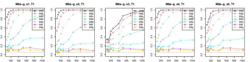
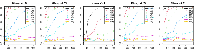
Figure 10: Empirical size (top) and power (bottom) of the tests for time-reversibility based on $T_{\rm TR1}^{(n,b,t)}$ described in Section 4.2. The upper plots and lower plots correspond to M8$a$–$g$ and M9$a$–$g$, respectively. Columns correspond to the weight functions $s_{1},\ldots,s_{5}$ from left to right, respectively. The horizontal axis of the plots corresponds to the parameters of models ($\lambda_{i}$ or $\gamma_{i}^{-1}$) and the vertical axis corresponds to empirical power.

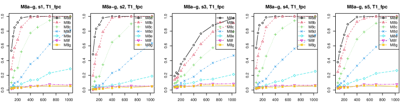
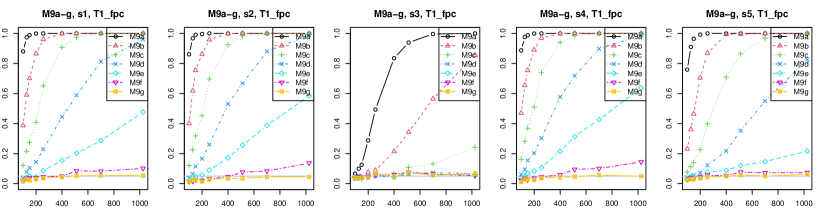
Figure 11: Empirical size (top) and power (bottom) of the tests for time-reversibility based on $T_{\rm TR1\_fpc}^{(n,b,t)}$ described in Section 4.2. The upper plots and lower plots correspond to M8$a$–$g$ and M9$a$–$g$, respectively. Columns correspond to the weight functions $s_{1},\ldots,s_{5}$ from left to right, respectively. The horizontal axis of the plots corresponds to the parameters of models ($\lambda_{i}$ or $\gamma_{i}^{-1}$) and the vertical axis corresponds to empirical power.

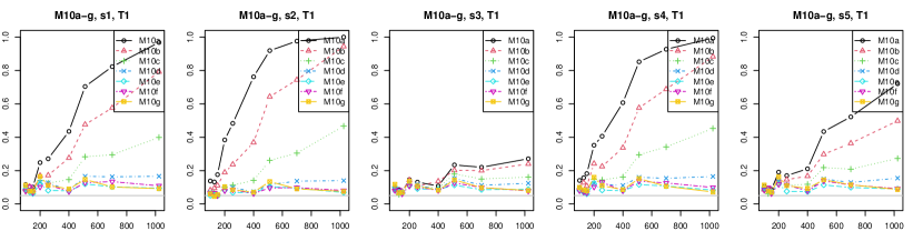
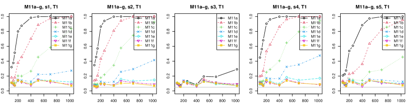
Figure 12: Empirical size (top) and power (bottom) of the tests for time-reversibility based on $T_{\rm TR1}^{(n,b,t)}$ described in Section 4.2. The upper plots and lower plots correspond to M10$a$–$g$ and M11$a$–$g$, respectively. Columns correspond to the weight functions $s_{1},\ldots,s_{5}$ from left to right, respectively. The horizontal axis of the plots corresponds to the parameters of models ($\lambda_{i}$ or $\gamma_{i}^{-1}$) and the vertical axis corresponds to empirical power.

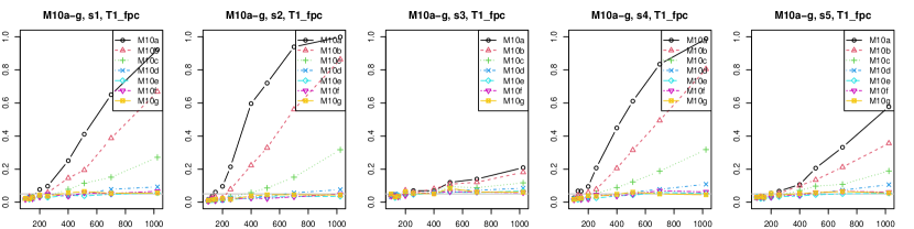
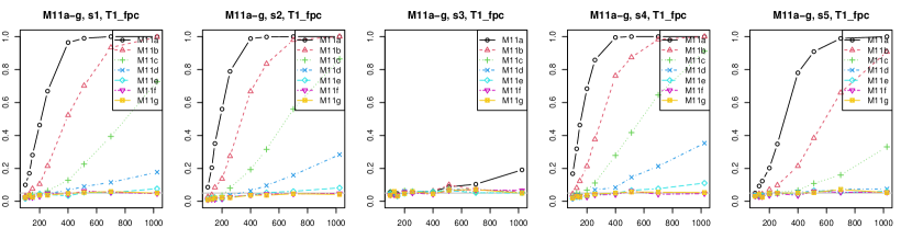
Figure 13: Empirical size (top) and power (bottom) of the tests for time-reversibility based on $T_{\rm TR1\_fpc}^{(n,b,t)}$ described in Section 4.2. The upper plots and lower plots correspond to M10$a$–$g$ and M11$a$–$g$, respectively. Columns correspond to the weight functions $s_{1},\ldots,s_{5}$ from left to right, respectively. The horizontal axis of the plots corresponds to the parameters of models ($\lambda_{i}$ or $\gamma_{i}^{-1}$) and the vertical axis corresponds to empirical power.

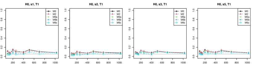
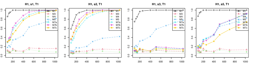
Figure 14: Empirical sizes (top, time-reversible models M0, M2, and M6a-c) and powers (bottom, time-irreversible models M1, M3, M4, M5, and M7a-c) as functions of $n$, of the tests for time-reversibility based on $T_{\rm TR1\_fpc}^{(n,b,t)}$ (without finite-population correction). Columns correspond to weight functions $s_{1},s_{2},s_{3},s_{5}$, respectively.

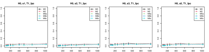
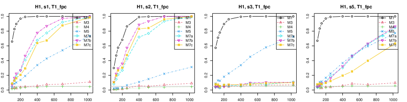
Figure 15: Empirical sizes (top, time-reversible models M0, M2, and M6a-c) and powers (bottom, time-irreversible models M1, M3, M4, M5, and M7a-c) as functions of $n$, of the tests for time-reversibility based on $T_{\rm TR1\_fpc}^{(n,b,t)}$ (with finite-population correction). Columns correspond to weight functions $s_{1},s_{2},s_{3},s_{5}$, respectively.

C.2 Additional simulation results for the test for asymmetry in tail dynamics

Here we provide additional simulation results with the same settings as in Figures 8 – 9 in the main manuscript but with weight functions $s_{1},s_{2},s_{3},s_{5}$.

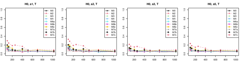
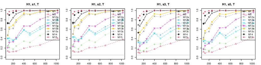
Figure 16: Empirical sizes (top) and powers (bottom), as functions of $n$, of the tests for tail symmetry based on $T_{\rm EQ}^{(n,b,t)}$ under various models. Columns correspond to weight functions $s_{1},s_{2},s_{3},s_{5}$, respectively.

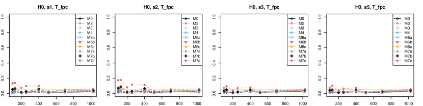
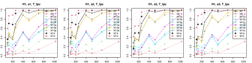
Figure 17: Empirical sizes (top) and powers (bottom), as functions of $n$, of the tests for tail symmetry based on $T_{\rm EQ\_fpc}^{(n,b,t)}$ (with finite–population correction) under various models. Columns correspond to weight functions $s_{1},s_{2},s_{3},s_{5}$, respectively.

References

- Anderson, (1993) Anderson, T. W. (1993). Goodness of fit tests for spectral distributions. The Annals of Statistics, pages 830–847.
- Baruník and Kley, (2019) Baruník, J. and Kley, T. (2019). Quantile coherency: A general measure for dependence between cyclical economic variables. The Econometrics Journal, 22(2):131–152.
- Beare and Seo, (2014) Beare, B. K. and Seo, J. (2014). Time irreversible copula-based markov models. Econometric Theory, pages 923–960.
- Birr et al., (2019) Birr, S., Kley, T., and Volgushev, S. (2019). Model assessment for time series dynamics using copula spectral densities: a graphical tool. arXiv:1804.01440.
- Birr et al., (2017) Birr, S., Volgushev, S., Kley, T., Dette, H., and Hallin, M. (2017). Quantile spectral analysis for locally stationary time series. Journal of the Royal Statistical Society: Series B, 79(5):1619–1643.
- Brillinger and Rosenblatt, (1967) Brillinger, D. and Rosenblatt, M. (1967). Computation and interpretation of kth order spectra. In Harris, B., editor, Spectral Analysis of Time Series, pages 189–232. John Wiley, New York.
- Brillinger, (1969) Brillinger, D. R. (1969). Asymptotic properties of spectral estimates of second order. Biometrika, 56(2):375–390.
- Brillinger, (1975) Brillinger, D. R. (1975). Time series: Data Analysis and Theory. Holt, Rinehart and Winston, Inc.
- Chen et al., (2000) Chen, Y.-T., Chou, R. Y., and Kuan, C.-M. (2000). Testing time reversibility without moment restrictions. J. Econometrics, 95(1):199–218.
- Dahlhaus, (1985) Dahlhaus, R. (1985). Asymptotic normality of spectral estimates. Journal of Multivariate Analysis, 16(3):412–431.
- Dahlhaus, (1988) Dahlhaus, R. (1988). Empirical spectral processes and their applications to time series analysis. Stochastic Processes and their Applications, 30(1):69–83.
- Davis and Mikosch, (2009) Davis, R. A. and Mikosch, T. (2009). The extremogram: A correlogram for extreme events. Bernoulli, 15(4):977–1009.
- Davis et al., (2013) Davis, R. A., Mikosch, T., and Zhao, Y. (2013). Measures of serial extremal dependence and their estimation. Stochastic Processes and their Applications, 123:2575–2602.
- De Gooijer, (2017) De Gooijer, J. G. (2017). Elements of nonlinear time series analysis and forecasting, volume 37. Springer.
- Dette et al., (2015) Dette, H., Hallin, M., Kley, T., Volgushev, S., et al. (2015). Of copulas, quantiles, ranks and spectra: An -approach to spectral analysis. Bernoulli, 21(2):781–831.
- Fermanian et al., (2004) Fermanian, J.-D., Radulovic, D., Wegkamp, M., et al. (2004). Weak convergence of empirical copula processes. Bernoulli, 10(5):847–860.
- Gaenssler et al., (2007) Gaenssler, P., Molnár, P., and Rost, D. (2007). On continuity and strict increase of the cdf for the sup-functional of a gaussian process with applications to statistics. Results in Mathematics, 51(1-2):51–60.
- Ghil et al., (2002) Ghil, M., Allen, M., Dettinger, M., Ide, K., Kondrashov, D., Mann, M., Robertson, A., Saunders, A., Tian, Y., Varadi, F., and Yiou, P. (2002). Advanced spectral methods for climate time series. Rev. Geophys., 2002:1003–1043.
- Granger and Hatanaka, (2015) Granger, C. W. J. and Hatanaka, M. (2015). Spectral Analysis of Economic Time Series. Princeton University Press.
- Grenander and Rosenblatt, (1957) Grenander, U. and Rosenblatt, M. (1957). Statistical analysis of stationary time series. John Wiley & Sons, New York.
- Hagemann, (2013) Hagemann, A. (2013). Robust spectral analysis (arxiv:1111.1965v2). ArXiv e-prints.
- Hallin et al., (1988) Hallin, M., Lefevre, C., and Puri, M. L. (1988). On time-reversibility and the uniqueness of moving average representations for non-gaussian stationary time series. Biometrika, 75(1):170–171.
- Han et al., (2014) Han, H., Linton, O., Oka, T., and Whang, Y.-J. (2014). The cross-quantilogram: measuring quantile dependence and testing directional preeictability between time series. available at: http://papers.ssrn.com/sol3/papers.cfm?abstract_id=2338468.
- Hong, (1999) Hong, Y. (1999). Hypothesis testing in time series via the empirical characteristic function: a generalized spectral density approach. Journal of the American Statistical Association, 94(448):1201–1220.
- Hong, (2000) Hong, Y. (2000). Generalized spectral tests for serial dependence. Journal of the Royal Statistical Society: Series B (Statistical Methodology), 62(3):557–574.
- Ibragimov, (1963) Ibragimov, I. A. (1963). On estimation of the spectral function of a stationary gaussian process. Theory of Probability & Its Applications, 8(4):366–401.
- Jondeau and Rockinger, (2003) Jondeau, E. and Rockinger, M. (2003). Testing for differences in the tails of stock-market returns. J. Empir. Finance, 10(5):559–581.
- Kley, (2014) Kley, T. (2014). Quantile-Based Spectral Analysis: Asymptotic Theory and Computation. PhD thesis, Ruhr-Universität Bochum.
- Kley, (2016) Kley, T. (2016). Quantile-based spectral analysis in an object-oriented framework and a reference implementation in R: The quantspec package. Journal of Statistical Software, 70(3):1–27.
- (30) Kley, T., Volgushev, S., Dette, H., Hallin, M., et al. (2016a). Quantile spectral processes: Asymptotic analysis and inference. Bernoulli, 22(3):1770–1807.
- (31) Kley, T., Volgushev, S., Dette, H., Hallin, M., et al. (2016b). Supplement to ”quantile spectral processes: Asymptotic analysis and inference”. Bernoulli, 22(3):1770–1807.
- Klüppelberg and Mikosch, (1996) Klüppelberg, C. and Mikosch, T. (1996). The integrated periodogram for stable processes. The Annals of Statistics, 24(5):1855–1879.
- Koenker and Xiao, (2006) Koenker, R. and Xiao, Z. (2006). Quantile autoregression. Journal of the American Statistical Association, 101(475):980–990.
- Kokoszka and Mikosch, (1997) Kokoszka, P. and Mikosch, T. (1997). The integrated periodogram for long-memory processes with finite or infinite variance. Stochastic processes and their applications, 66(1):55–78.
- Krupskii and Joe, (2019) Krupskii, P. and Joe, H. (2019). Nonparametric estimation of multivariate tail probabilities and tail dependence coefficients. J. Multivar. Anal., 172:147–161.
- Lange et al., (2019) Lange, H., Brunton, S., and Kutz, N. (2019). Spectral Methods for Time Series Prediction with Application to Fluid Flows. In APS Division of Fluid Dynamics Meeting Abstracts, APS Meeting Abstracts, page Q41.008.
- Lee and Rao, (2012) Lee, J. and Rao, S. S. (2012). The probabilistic spectral density. Personal Communication.
- Li and Genton, (2013) Li, B. and Genton, M. G. (2013). Nonparametric identification of copula structures. J. Amer. Statist. Assoc., 108(502):666–675.
- Li, (2008) Li, T.-H. (2008). Laplace periodogram for time series analysis. Journal of the American Statistical Association, 103(482):757–768.
- Li, (2012) Li, T.-H. (2012). Quantile periodograms. Journal of the American Statistical Association, 107(498):765–776.
- Li, (2013) Li, T.-H. (2013). Time Series with Mixed Spectra: Theory and Methods. CRC Press, Boca Raton.
- Li, (2021) Li, T.-H. (2021). Quantile-frequency analysis and spectral measures for diagnostic checks of time series with nonlinear dynamics. J. R. Stat. Soc. Ser. C Appl. Stat., 70(2):270–290.
- Likkason, (2011) Likkason, O. (2011). Spectral Analysis of Geophysical Data.
- Lim and Oh, (2021) Lim, Y. and Oh, H.-S. (2021). Quantile spectral analysis of long-memory processes. Empirical Economics, pages 1–22.
- Linton and Whang, (2007) Linton, O. and Whang, Y.-J. (2007). The quantilogram: with an application to evaluating directional predictability. Journal of Econometrics, 141:250–282.
- Mangold, (2017) Mangold, B. (2017). New concepts of symmetry for copulas. Technical report, FAU Discussion Papers in Economics.
- Mikosch and Norvaiša, (1997) Mikosch, T. and Norvaiša, R. (1997). Uniform convergence of the empirical spectral distribution function. Stochastic processes and their applications, 70(1):85–114.
- Nelsen, (1993) Nelsen, R. B. (1993). Some concepts of bivariate symmetry. J. Nonpara. Statist., 3(1):95–101.
- Nelsen, (2006) Nelsen, R. B. (2006). An introduction to copulas. Springer Science & Business Media.
- Neumann and Paparoditis, (2008) Neumann, M. H. and Paparoditis, E. (2008). Simultaneous confidence bands in spectral density estimation. Biometrika, 95(2):381–397.
- Paparoditis and Politis, (2002) Paparoditis, E. and Politis, D. N. (2002). The local bootstrap for markov processes. J. Stat. Plan. Inf., 108(1-2):301–328.
- Politis et al., (1999) Politis, D. N., Romano, J. P., and Wolf, M. (1999). Subsampling. Springer.
- Priestley, (1987) Priestley, M. B. (1987). Spectral analysis and time series. Academic press.
- Ramsey and Rothman, (1996) Ramsey, J. B. and Rothman, P. (1996). Time irreversibility and business cycle asymmetry. J. Money Credit Bank., 28(1):1–21.
- Rosco and Joe, (2013) Rosco, J. and Joe, H. (2013). Measures of tail asymmetry for bivariate copulas. Stat. Pap., 54(3):709–726.
- Rudin et al., (1964) Rudin, W. et al. (1964). Principles of mathematical analysis, volume 3. McGraw-Hill New York.
- Segers, (2012) Segers, J. (2012). Asymptotics of empirical copula processes under non-restrictive smoothness assumptions. Bernoulli, 18(3):764–782.
- Sklar, (1959) Sklar, M. (1959). Fonctions de répartition à n dimensions et leurs marges. Publ. Inst. Statist. Univ. Paris, 8:229–231.
- So and Chan, (2014) So, M. K. and Chan, R. K. (2014). Bayesian analysis of tail asymmetry based on a threshold extreme value model. Comput. Stat. Data Anal., 71:568–587.
- Su et al., (2021) Su, X., Zhan, W., and Li, Y. (2021). Quantile dependence between investor attention and cryptocurrency returns: evidence from time and frequency domain analyses. Applied Economics.
- Van der Vaart, (2000) Van der Vaart, A. W. (2000). Asymptotic statistics, volume 3. Cambridge university press.
- van der Vaart and Wellner, (1996) van der Vaart, A. W. and Wellner, J. A. (1996). Weak Convergence and Empirical Processes. Springer.
- Vervaat, (1972) Vervaat, W. (1972). Functional central limit theorems for processes with positive drift and their inverses. Probability Theory and Related Fields, 23(4):245–253.
- von Sachs, (2020) von Sachs, R. (2020). Nonparametric spectral analysis of multivariate time series. Annual Review of Statistics and Its Application, 7(1):361–386.
- Wu and Shao, (2004) Wu, W. B. and Shao, X. (2004). Limit theorems for iterated random functions. Journal of Applied Probability, 41(2):425–436.