Analysis of a Tau Neutrino Origin for the Near-Horizon Air Shower Events Observed by the Fourth Flight of the Antarctic Impulsive Transient Antenna (ANITA)

Abstract

We study in detail the sensitivity of the Antarctic Impulsive Transient Antenna (ANITA) to possible $\nu_{\tau}$ point source fluxes detected via $\tau$-lepton-induced air showers. This investigation is framed around the observation of four upward-going extensive air shower events very close to the horizon seen in ANITA-IV. We find that these four upgoing events are not observationally inconsistent with $\tau$-induced EASs from Earth-skimming $\nu_{\tau}$ both in their spectral properties as well as in their observed locations on the sky. These four events as well as the overall diffuse and point source exposure to Earth-skimming $\nu_{\tau}$ are also compared against published ultrahigh-energy neutrino limits from the Pierre Auger Observatory. While none of these four events occured at sky locations simultaneously visible by Auger, the implied fluence necessary for ANITA to observe these events is in strong tension with limits set by Auger across a wide range of energies and is additionally in tension with ANITA’s Askaryan in-ice neutrino channel above $10^{19}$ eV. We conclude by discussing some of the technical challenges with simulating and analyzing these near horizon events and the potential for future observatories to observe similar events.

I Introduction

The fourth flight of ANITA (ANITA-IV) observed four below-horizon cosmic ray-like events that have non-inverted polarity - a 3.2 $\sigma$ fluctuation if due to background [1]. Unlike the steeply-upcoming ($\sim 30^{\circ}$ below the radio horizon) anomalous events of this type reported in two previous ANITA flights [2, 3], all of the ANITA-IV anomalous events are observed at angles close to the horizon ($\lesssim 1^{\circ}$ below the horizon).

A Standard Model explanation originally proposed for the steeply upcoming events from the first and third ANITA flights (ANITA-I and ANITA-III, respectively) was skimming $\nu_{\tau}$ interactions in the Earth producing $\tau$ leptons that escape into the atmosphere, subsequently decaying and producing an upgoing extensive air shower (EAS). While this origin was initially considered to be unlikely due to the attenuation of neutrinos across the long chord lengths through Earth at these steep angles, several analyses have studied the $\nu_{\tau}$-origin hypothesis for these steeply upgoing events [2, 4].

These analyses have studied two different astrophysical assumptions: (1) that the events were due to a diffuse isotropic flux of ultra-high energy (UHE) neutrinos; and (2) that the events were from transient UHE neutrino point sources that were active or flaring during each flight.

Under the diffuse hypothesis for the ANITA-I & ANITA-III anomalous events, a prior analysis by the ANITA collaboration [5, 6] implied a diffuse neutrino flux limit that is in strong tension with the limits imposed by the IceCube [7] and Pierre Auger [8] observatories (Auger).

A preliminary follow-up analysis by the ANITA collaboration estimated the sensitivity of ANITA to $\nu_{\tau}$ point sources in the direction of the ANITA-I and ANITA-III anomalous events to investigate the possibility that a point-like neutrino source could be responsible for these events. This analysis bounded the instantaneous point source effective area to $\lesssim$ 2.2 m² for the ANITA-I event and $\lesssim$ 0.3 m² for the ANITA-III event [9]. These values are significantly smaller than Auger’s $\nu_{\tau}$ point source peak effective area to $\nu_{\tau}$ of $1\times 10^{4}$ to $3\times 10^{5}$ m² for energies above $10^{17}$ eV and are also in strong tension with point-like neutrino limits set by Auger [10]

A number of alternative hypothesis have been proposed to explain the ANITA-I and ANITA-III anomalous events. These range from Beyond Standard Model (BSM) physics [11, 12, 13, 14, 15, 16, 17, 18, 19] to more mundane effects such as transition radiation of cosmic ray air showers piercing the Antarctic ice sheet [20] and subsurface reflections due to anomalous ice features [21] although the latter has recently been experimentally constrained by the ANITA collaboration [22].

ANITA’s sensitivity to the $\tau$ EAS channel is highly directional and is maximal near the horizon where it is orders of magnitude larger than for the steeply upgoing angles of the ANITA-I and ANITA-III events. This opens the possibility for an Earth-skimming $\nu_{\tau}$ explanation for the ANITA-IV events (that occur extremely close to the horizon) while potentially significantly reducing the tension with limit set by Auger and IceCube.

The detection of this new class of events, not observed in previous ANITA flights, is consistent with the improvements in ANITA-IV’s sensitivity [23]. In this paper we update the previous ANITA $\nu_{\tau}$ EAS sensitivity analysis [5, 6] to estimate the diffuse and point source transient fluxes implied by this new class of events and compare them with the limits imposed by other neutrino observatories.

The paper is organized as follows: in §II we summarize the properties of the ANITA-IV anomalous events relevant to this analysis; in §III, we present the simulation framework used to estimate ANITA’s sensitivity to $\tau$ neutrinos, via in-air $\tau$ decays, including a discussion of the models used for the air shower radio emission and detector response. The results of this analysis are presented in §IV and detailed discussions and conclusions are provided in §V and §VI, respectively.

II ANITA-IV Anomalous Events

While ANITA was originally designed to detect the Askaryan emission from in-ice UHE neutrino interactions, ANITA is also sensitive to the geomagnetic radiation emitted by ultrahigh-energy cosmic ray (UHECR) induced extensive air showers (EAS) as they develop in the atmosphere. As an extensive air shower evolves in the presence of the Earth’s magnetic field, charged particles in the shower are accelerated via the Lorentz force, creating a time-varying transverse current within the shower. This transverse current generates an impulsive electric field whose polarization is transversely aligned with the orientation of the Earth’s magnetic field. Over Antarctica, the Earth’s magnetic field is primarily vertical, resulting in predominately horizontally-polarized emission from an EAS [24].

Typical air shower events observed by ANITA are classified into two categories: (1) direct UHECR events that reconstruct above the radio horizon (i.e. ANITA observes the emission directly from the shower at it develops in the atmosphere); and (2) reflected UHECR events where ANITA observes the radio emission from air showers after the radio emission has reflected off the surface of Antarctica (these must therefore reconstruct below the horizon).

Along with their reconstructed direction, events are also typically classified as direct or reflected by the polarity of the received electric field. For a unipolar waveform, the polarity is determined by the sign ($\pm$) of the impulse. For bipolar waveforms, the polarity is typically indicated by the order of the two primary poles (i.e. $+,-$ or $-,+$). Due to the Fresnel reflection coefficient at the air-ice boundary, reflected EAS signals have a completely inverted polarity with respect to the signals observed directly from an EAS without reflection [25]. Polarity, which is related to the sign of the electric field impulse, is distinct from polarization, which describes the geometric orientation of the electric field and is used to separate EAS events from in-ice Askaryan neutrino events. Over its four flights, ANITA has observed seven direct events and 64 reflected UHECR events [26, 25, 1].

ANITA-IV also observed four extensive air shower-like events that have the same polarity as the direct events (i.e. non-inverted $\implies$ non-reflected), but reconstruct below the horizon. These four events therefore appear to be upward-going air showers emerging from the surface of the Earth, but unlike the ANITA-I and ANITA-III anomalous events, the ANITA-IV events reconstruct near to, but below the horizon ($\lesssim 1^{\circ}$) [1]. As shown in Table 1, ANITA’s angular uncertainty for these events is $\sim 0.2^{\circ}$, placing these events typically $\gtrsim 1\sigma$ to $4\sigma$ below the horizon.

The significance of finding 4 events with a polarity inconsistent with their geometry out of the 27 air shower events with a well-determined polarity is estimated to be greater than 3 $\sigma$, when considering the possibilities that: the events could be an anthropogenic background; that there might be an error in the reconstructed arrival direction; and that the polarity might be misidentified [1]. The probability distribution of the true number of non-inverted EAS-like events from one of the two Monte Carlo simulations used to evaluate the above significance is shown in Table 1. The most probable number of true signal events, under the above background possibilities, is three with total probability density of 0.7 (against the probability of observing 0, 1, 2, or 4 signal events).

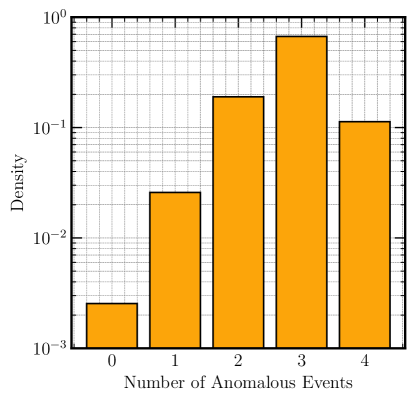
Figure 1: The probability density distribution (i.e. normalized event density) for the true number of EAS signal events observed by ANITA-IV under the assumptions of the toy Monte Carlo simulations described in [1]

.

While the significance of the observed anomalies do not clearly distinguish these events from possible backgrounds, in this study we consider the hypothesis that these events may be due to a tau neutrino interaction inside the Earth that creates an exiting $\tau$ lepton and analyze these events under this hypothesis.

The observed event parameters for the ANITA-IV anomalous events under the hypothesis of a tau-neutrino origin are shown in Table 1 where $\theta$ is the elevation angle of the observed radio-frequency direction and $\theta_{H}$ is the elevation angle of the radio horizon.

Table 1: The time of each observed event along with the reconstructed elevation angle of the shower, $\theta$, below the radio horizon, $\theta_{H}$. All events are observed within $1^{\circ}$ of the radio horizon and are all greater than $1\sigma$ from the horizon.

Event	Time (ISO 8601)	$(\theta-\theta_{H})$ (deg.)
4098827	2016-12-03T10:03:27Z	-0.25$\pm$0.21∘
19848917	2016-12-08T11:44:54Z	-0.65$\pm$0.20∘
50549772	2016-12-16T15:03:19Z	-0.81$\pm$0.20∘
72164985	2016-12-22T06:28:14Z	-0.19$\pm$0.10∘

III ANITA’s Sensitivity to Tau Neutrinos via Extensive Air Showers

In this section we estimate the sensitivity of ANITA to tau neutrinos via the extensive air shower channel for both diffuse and point source fluxes. A flux density of tau neutrinos $F(t,E_{\nu},\hat{r})$ arriving on Earth (i.e. the number of events per unit area per unit solid angle per unit time per unit energy) depends on sky direction $\hat{r}$, and varies with neutrino energy $E_{\nu}$ and time $t$. The differential contribution to the number of events $N_{obs}$ detected with a given observatory is shown in Equation 1.

$$\begin{split}\frac{dN_{obs}}{dt\ dE_{\nu}\ d\Omega\ dA}=({\hat{r}_{\nu}}\cdot\hat{x}_{E})\ &\Theta(\hat{r}\cdot\hat{x}_{E})\\ &F(t,E_{\nu},\hat{r})\ P_{obs}(t,E_{\nu},\hat{r},\vec{x}_{E}).\end{split}$$ (1)

where:

$dN_{obs}$ ${}={}$	the differential number of observed events,
$dA$ ${}={}$	the differential area we consider,
$t$ ${}={}$	the observation time,
$dt$ ${}={}$	the differential observation time interval,
$E_{\nu}$ ${}={}$	the neutrino energy,
$dE_{\nu}$ ${}={}$	the differential neutrino energy band,
$\hat{r}_{\nu}$ ${}={}$	the vector point towards the neutrino source,
$\vec{x}_{E}$ ${}={}$	the location of the differential area on the surface of the Earth,
$\Theta$ ${}={}$	the Heaviside step-function,
$F(t,E_{\nu},\hat{r})$ ${}={}$	the incident flux of tau neutrinos,
$P_{obs}(t,E_{\nu},\hat{r},\vec{x}_{E})$ ${}={}$	the probability that this event is detected by this observatory.

The behavior specific to the observatory is encoded in the function $P_{obs}(t,E_{\nu},\vec{x}_{E},\hat{r})$, which is the probability that a tau neutrino with energy $E_{\nu}$ coming from sky direction $\hat{r}$ whose axis of propagation intersects a point $\vec{x}_{E}$ on the surface of integration $A$ (the surface of the Earth for ANITA) at time $t$ is observed. The dot product $\hat{r}\cdot\hat{x}_{E}$ accounts for the projected area element in the direction of $\hat{r}$ and $\Theta(\hat{r}\cdot\hat{x}_{E})$ accounts for the fact that we only consider neutrinos propagation axes that exit the Earth in the observing regions of interest.

A full description of the function $P_{obs}$ for ANITA is derived for a diffuse flux in [5, 6] and is extended for neutrino point sources in Equation 2. The probability of observation is decomposed into a convolution of probabilities summarized as follows: 1) the probability, $P_{\mathrm{exit}}$, that a $\nu_{\tau}$ with original energy $E_{\nu}$ undergoes a sequence of interactions inside the Earth that results in a $\tau$ lepton leaving the Earth; 2) the probability, $P_{\mathrm{decay}}$, that the $\tau$ lepton subsequently propagates in the atmosphere and decays before reaching ANITA [9]; 3) that the $\tau$ decay creates a shower with sufficient energy to be detectable by ANITA and that the decay point is far away enough from ANITA that the shower can fully develop before passing ANITA; and 4) the probability, $P_{\mathrm{trig}}$, that the radio emission from this particular shower is sufficiently strong enough to trigger ANITA (and be detected) [27, 5, 6]. All of these factors are combined later in this article to calculate ANITA’s effective area to $\tau$-induced extensive air showers (Equation 2) given a $\nu_{\tau}$ of energy $E_{\nu}$ coming from direction $\hat{r}_{\nu}$ at time $t$ with the $\tau$ exiting the earth at $\vec{x}_{E}$.

$$P_{obs}(t,E_{\nu},\hat{r},\vec{x}_{E})= \int dE_{\tau}\ P_{exit}\left(E_{\tau}\ |\ E_{\nu},\theta_{em}\right)$$ (2)

$$\int ds_{decay}\ P_{decay}\left(s_{decay}\ |\ E_{\tau}\right)$$

$$\int dE_{EAS}\ P_{EAS}\left(E_{EAS}\ |\ E_{\tau}\right)$$

$$\int d\mathcal{E}\ P_{\mathcal{E}}\left(\mathcal{E}\ |\ E_{EAS},s_{decay},\hat{r}_{\nu},\right)$$

$$\quad\quad\ \ P_{trig}\left(\vec{x}_{\mathrm{ANITA}}\ |\ \mathcal{E},s_{decay},\hat{r}_{\nu}\right)$$

where:

$E_{\tau}$ ${}={}$	the energy of the exiting $\tau$,
$\theta_{em}$ ${}={}$	the emergence angle of $\tau$ at the surface,
$s_{decay}$ ${}={}$	the decay length of the $\tau$,
$E_{EAS}$ ${}={}$	the energy of the extensive air shower,
$\mathcal{E}$ ${}={}$	the electric field at the payload (V/m),
$\vec{x}_{\mathrm{ANITA}}$ ${}={}$	the location of ANITA,
$\hat{r}_{\nu}$ ${}={}$	the incident direction of the neutrino and $\tau$,

In §III.1 we provide some details of recent updates to the simulation components that were previously used to estimate the diffuse flux sensitivity of ANITA-I and ANITA-III [5, 9]. Namely, the sampling of tau decay modes, the look-up tables of electric fields produced with ZHAireS, and significant refinements to the ANITA-IV detector model. §III.2 reviews the detector acceptance calculation used for estimating the sensitivity to a diffuse neutrino flux and §III.3 develops the detector point source effective area formalism used to estimate ANITA’s sensitivity to a point source flux.

III.1 Models

The models used to evaluate ANITA’s acceptance to tau neutrinos via the extensive air shower channel were first developed in [5, 9]. In this section, we discuss the improvements that have been made to these models in this latest simulation to improve fidelity. For more detail and verification on the underlying models, we point the reader to the aforementioned references.

III.1.1 Tau Decays

In the ANITA tau neutrino acceptance bounds of [5, 6], a single $\tau$ decay was used ($\tau^{-}\to\pi^{-}\pi_{0}\nu_{\tau}$) with 99% of the energy going to showering particles to seed the air shower simulations. For this analysis and in [9], a large sample of $\tau^{-}$ decays with negative helicity were sampled using PYTHIA 8.244 [28]. For each sample, we estimated the total fraction of initial energy that goes into the EAS by excluding neutrinos and muons from the secondary particles. The resulting fraction of the original $\tau$ energy transferred to the air shower is shown in Figure 2.

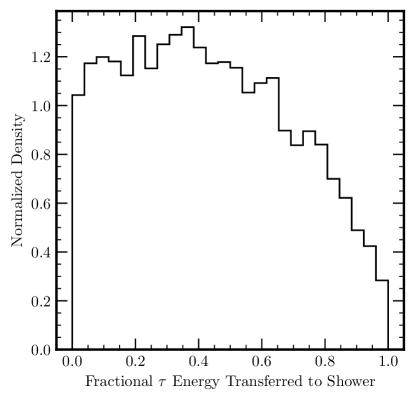
Figure 2: The relative fraction of the tau energy transferred to the shower in decays of ultrahigh-energy negative helicity $\tau$-leptons simulated using PYTHIA 8.244 [28, 5, 6].

III.1.2 Air Shower Electric Field Model

The previous ANITA-I & ANITA-III $\nu_{\tau}$ analysis used a simplified electric field model accounting only for the peak value of the electric field based on a large sample of ZHAireS [27] simulations. These were run at a full range of decay altitude ($0-9$ km in 1 km steps), emergence angles ($1^{\circ}-35^{\circ}$), and off-axis view angles, $\psi$ ($0^{\circ}-3^{\circ}$) completely covering the amplitude range detectable by ANITA. For this new work, this model was significantly improved by storing the complete time-domain electric field waveform (see Figure 3 and Figure 4 for an example). This EAS shower library was then used to produce a pair of 4D lookup-table (LUT) of electric field in terms of $(h_{decay},\theta_{em},\phi,f)$ or $(h_{decay},\theta_{em},\phi,t)$ where $\theta_{em}$ is the emergence angle of the $\tau$ at the exit location on the surface. All showers were simulated with a shower energy of 100 PeV. The electric field amplitude for EAS scales very close to linearly with shower energy across the energy range of interest[25, 27].

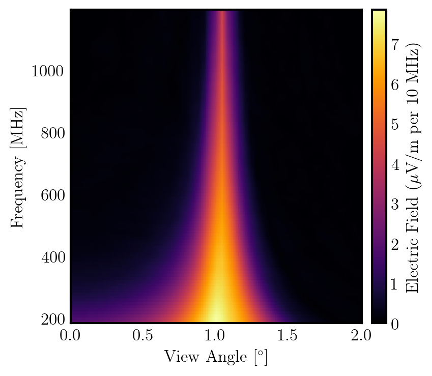
Figure 3: The electric field strength as a function of frequency and view angle with respect to the shower axis for a specific slice through the 4-D lookup table used to evaluate the electric field ($\theta_{\mathrm{em}}=5^{\circ}$, $h_{\mathrm{decay}}=2$ km).

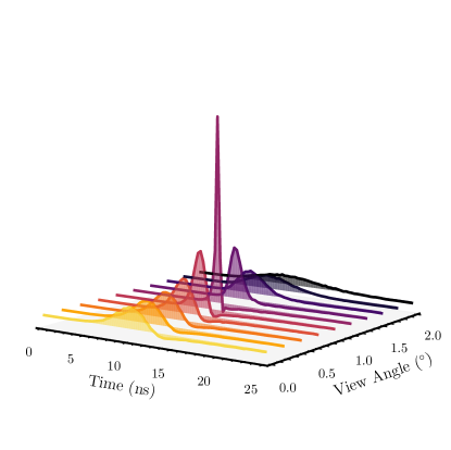
Figure 4: ZHAireS-simulated electric field waveforms for various view angles for a specific slice through the 4-D lookup table used to evaluate the electric field ($\theta_{\mathrm{em}}=5^{\circ}$, $h_{\mathrm{decay}}=2$ km).

$h_{decay}$, $\theta_{z}$, and $\phi$ are known a priori based upon the geometric properties of the specific simulation or Monte Carlo trial. These parameters are then used to perform a 4D quad-linear interpolation into the lookup-table to estimate the electric field at the payload. This field was then used as the primary input to the antenna and detector model with appropriate scaling to account for the specific shower energy that was being simulated.

III.1.3 Detector Model

The previous diffuse $\nu_{\tau}$ analysis used a detector model implemented in the frequency domain and assumed a constant frequency-independent boresight gain for ANITA’s quad-ridged horn antennas and ignored any off-axis effects due to the antenna beamwidth [5]. For this work, we have developed a completely new time-domain detector model based on a recent measurement of the impulse responses of all 96 channels in ANITA-IV [1] and flight-data-driven noise model, along with additional detector model improvements.

This new time-domain detector model directly uses in-flight data and post-flight calibration measurements and as such is expected to have much higher fidelity than the simple assumptions used in the frequency domain model of [5].

During the ANITA-IV EAS and neutrino analysis presented in [1], a detailed calibration campaign was performed to measure the total time-domain transfer function of every channel and configuration of the ANITA-IV payload. ANITA-IV had 96 channels (48 antennas each with two polarizations per antenna), however the payload also included dynamic notch filters on each channel, that were reconfigured during the flight, to combat radio-frequency interference. These notch filters can significantly change the amplitude and phase response of each individual channel; 6 different filter configurations were used throughout the flight for a total of $\sim 600$ independent impulse responses.

The payload-wide average of these responses for each configuration is shown in Figure 5. These measurements provide the total time-domain transfer function of each channel (including antennas, front-end LNAs, bandpass filters, notch filters, and second-stage signal chain). Since the transfer-function, $\bar{h}(t)$, is a complete representation of the ANITA signal chain from the antenna to the digitizer, the incident electric field can be immediately converted into a voltage via

$$V(t)=\bar{h}(t)*\mathcal{E}(t)$$ (3)

where:

$V(t)$ ${}={}$	the time-domain voltage measured by ANITA (in V),
$\bar{h}(t)$ ${}={}$	the time-domain transfer function (in m/ns),
$\mathcal{E}(t)$ ${}={}$	the time-domain incident electric field (in V/m),
${}={}$	represents linear convolution,

To calculate the observed waveform for a given channel, we convolve the time-domain electric field from the 4D ZHAireS interpolation (described in §III.1.2) with the specific time-domain response for that channel.

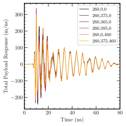
Figure 5: The average time-domain full signal chain transfer function for each notch filter configuration used in the ANITA-IV flight. The legend indicates the frequencies (in MHz) that each of the three filter notches were programmed to for each configuration.

For the time-domain model, we replace the analytic noise generation model used in the previous ANITA $\nu_{\tau}$ analysis with a model derived from actual GPS-triggered noise waveforms recorded during the ANITA-IV flight. We extracted a large sample of so called “minimum-bias” events from each of the $\sim$300 runs in the ANITA-IV flight dataset. Since the bin-by-bin amplitude of random phasor noise in the frequency domain is expected to follow a Rayleigh distribution, we fit a Rayleigh probability density function to each 5 MHz bin in the distribution of amplitude spectral densities using a maximum-likelihood estimator (see [29] for more details on this process). The amplitude spectral density of background noise evolved significantly throughout the flight (Figure 6), so this fitting process is done on a run-by-run basis.

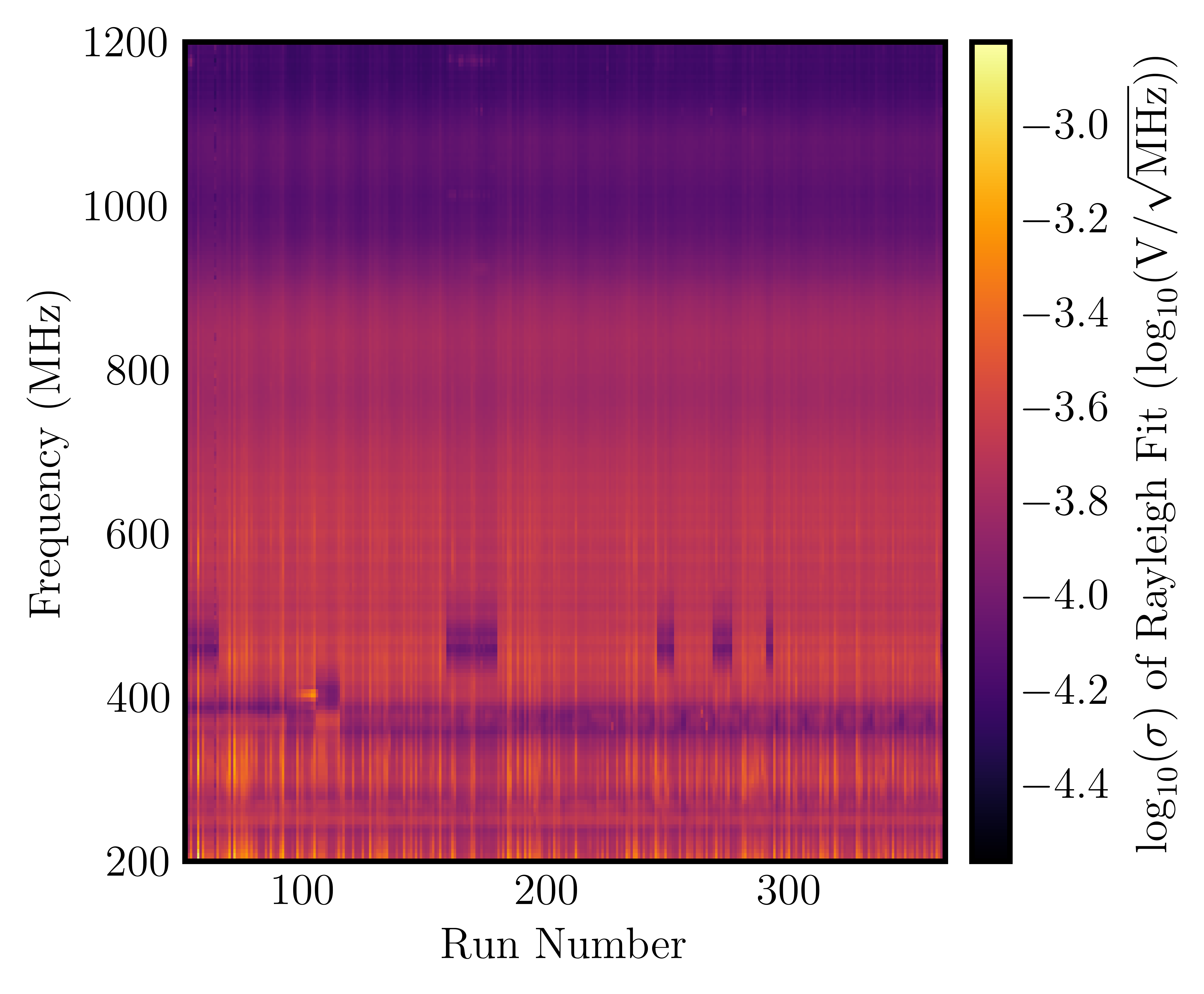
Figure 6: The average per-channel integrated noise power for each run of the ANITA-IV flight shown as the logarithm of the scale parameter, $\sigma$, of a Rayleigh distribution fit to the distribution of noise samples in a given frequency bin over a given run. The changing center frequency of the notch filters is clearly evident as changes in the location of the “horizontal” stripes in this figure.

Given a simulated EAS signal waveform calculated using Equation 3 and a random noise waveform sampled from the fitted Rayleigh distributions, the signal-to-noise ratio (SNR), used in our trigger calculation, is calculated with Equation 4.

$$\begin{split}\mathrm{SNR}=&\frac{\max{V(t)}-\min{V(t)}}{2\sigma}\\ =&\frac{\max{V(t)}-\min{V(t)}}{2\sqrt{\sum_{t}V_{n}(t)^{2}}}\end{split}$$ (4)

where:

$SNR$ ${}={}$	signal-to-noise ratio,
$V(t)$ ${}={}$	the time-domain signal voltage,
$\sigma$ ${}={}$	the standard deviation of the noise waveform,
$V_{n}(t)$ ${}={}$	the simulated noise waveform

Trigger Model

Given the observed SNR of a particular simulated event, we model ANITA’s trigger using a Heaviside step-function where $P_{\mathrm{trig}}=100\%$ for any trial with $\mathrm{SNR}>\mathrm{SNR}_{\mathrm{trig}}$ and $P_{\mathrm{trig}}=0\%$ otherwise. The threshold signal-to-noise ratio, SNR_trig, is chosen as the minimum value of the distribution of SNRs of the total population of EAS observed by ANITA-IV during post-flight analysis (Figure 7). This was chosen to emulate both the hardware trigger as well as the analysis efficiency and cuts employed by ANITA-IV to isolate UHECR signal events.

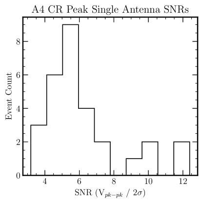
Figure 7: The peak single-antenna signal-to-noise ratio (SNR) for each of the 28 cosmic ray observed by ANITA-IV. $\sigma$ is the RMS of thermal noise measured in the corresponding channel

In the following sections, we present the formalism used to calculate ANITA-IV’s effective area and exposure to $\tau$-induced EAS and present the results of these simulations for both diffuse and point-source $\nu_{\tau}$ fluxes.

III.2 Acceptance to a Diffuse and Isotropic Flux

We model a diffuse, isotropic flux as independent of direction and time so that we may write $F(t,E_{\nu},\hat{r})\simeq F(E_{\nu})$. Equation 1 then becomes

$$\begin{split}\frac{dN_{obs}}{dt\ dE_{\nu}\ dA\ d\Omega}=(\hat{r}_{\star}\cdot\hat{x}_{E})\ &\Theta(\hat{r}_{\star}\cdot\hat{x}_{E})\\ &F(E_{\nu})\ P_{obs}(t,E_{\nu},\hat{r}_{\star},\vec{x}),\end{split}$$ (5)

where $\hat{r}_{\star}$ is a fixed direction on the sky. Since a diffuse isotropic flux, $F(E_{\nu})$, does not explicitly depend on the differential area of integration $dA$ or projected differential solid angle $d\Omega$, we may write

$$\frac{dN_{obs}}{dt\ dE_{\nu}}=F(E_{\nu})\ \langle A\Omega\rangle(t,E_{\nu}),$$ (6)

where the acceptance $A\Omega(t,E_{\nu})$, averaged over the sky, is given by

$$\begin{split}\langle A\Omega\rangle(t,E_{\nu})=&\int_{\Omega}d\Omega\\ &\int_{A}dA\ \hat{r}_{\star}\cdot\hat{x}_{E}\ \Theta(\hat{r}\cdot\hat{x}_{E})\ \ P_{obs}(t,E_{\nu},\hat{r}_{\star},\vec{x}),\end{split}$$ (7)

This is based on the formalism used in [5, 6] but we have rederived it here with an explicit time dependence to enforce a clear connection with the point source effective area, derived in the next section. While the flux is independent of time, ANITA’s acceptance, $\langle A\Omega\rangle(t)$, still has an explicit time dependence due to variations in $dA$ and $P_{obs}$ throughout the $\sim 30$-day ANITA flight.

III.3 Point Source Effective Area

We model a point source flux in a fixed sky direction $\hat{r}_{\star}$ as

$$S(t,E_{\nu},\hat{r}_{\star})=\int d\Omega\ \delta(\hat{r}-\hat{r}_{\star})\ F(t,E_{\nu},\hat{r}),$$ (8)

where $\delta(\hat{r}-\hat{r}_{\star})$ is a Dirac $\delta$-function on a spherical surface with units of inverse steradians. Unlike a diffuse and isotropic flux, point source flux is in units of number per unit time per unit energy per unit area. Applying the integration over solid angle in Equation 1, the event rate for the point source is given by

$$\begin{split}\frac{dN_{obs}}{dt\ dE_{\nu}\ dA}=(\hat{r}_{\star}\cdot\hat{x}_{E})\ &\Theta(\hat{r}_{\star}\cdot\hat{x}_{E})\ \\ &S(t,E_{\nu},\hat{r}_{\star})\ P_{obs}(t,E_{\nu},\hat{r}_{\star},\vec{x}).\end{split}$$ (9)

Since the point source flux $S(t,E_{\nu},\hat{r}_{\star})$ also does not explicitly depend on the differential area of integration $dA$ used for estimating the event rate, we may write

$$\frac{dN_{obs}}{dt\ dE_{\nu}}=S(t,E_{\nu},\hat{r}_{\star})\langle A\rangle(t,E_{\nu},\hat{r}_{\star}),$$ (10)

where the point source effective area $A(t,E_{\nu},\hat{r}_{\star})$ is given by

$$\begin{split}A(t,E_{\nu},\hat{r}_{\star})=\int_{A_{g}}dA_{g}\ (\hat{r}_{\star}\cdot\hat{x}_{E})\ &\Theta(\hat{r}_{\star}\cdot\hat{x}_{E})\\ &P_{obs}(t,E_{\nu},\hat{r}_{\star},\vec{x}),\end{split}$$ (11)

where $A_{g}$ is the geometric area on the surface of the Earth that we integrate over (yellow spherical patch in Figure 8). For ANITA’s $\nu_{\tau}$ effective area, we define $A_{g}$ as the ellipsoidal area on the surface from which the off-axis view angle at the surface, $\theta_{\mathrm{view,exit}}$, is less than some predefined $\theta_{\mathrm{max}}$. In most cases, $\theta_{\mathrm{max}}\sim 1-2^{\circ}$ (Figure 8.

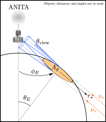
Figure 8: A diagram showing how this analysis defines the geometric area as the area on the surface of the Earth which ANITA observes with a view angle from the surface of less than $\theta_{{\mathrm{view,max}}}$.

III.4 tapioca

To simulate ANITA’s sensitivity to both diffuse and point sources of $\tau$ neutrinos using the formalism in §III.3, we have developed a new $\nu_{\tau}$ simulation code, the Tau Point Source Calculator, or tapioca. tapioca is publicly available and released under an open-source copy-left license.

In particular, tapioca performs a Monte Carlo evaluation of the integrals shown in Equations 7 and 11. A flow chart showing the top-level logic of the tapioca code, as well as the required inputs and data sources, is shown in Figure 9 and described in the remainder of this section.

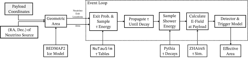
Figure 9: A flowchart showing the top-level logic and event loop of the tapioca simulation code with the external data sources used at each stage. This logic is described in detail in Section III.4 of the text.

Given the location of the payload ($\phi,\lambda,h,t$), where $\phi,\lambda$ are latitude and longitude, $h$ is the altitude above the reference Earth ellipsoid, and $t$ is the observation, and the coordinates of a neutrino source ($\alpha,\delta$), we calculate the geometric area of neutrino exit locations that is potentially detectable by ANITA. This is done by setting a cut on the maximum view angle, $\theta_{\mathrm{view,exit}}$, at the neutrino exit location on the surface as shown in Figure 8.

Since the observed ANITA-IV events are extremely close to the horizon, we must accurately take into account the altitude of the ice and curvature of the Earth at the observed location of each event. For each observed ANITA-IV event, we raytrace the observed RF direction back to the continent and then use the BEDMAP2 [30] ice dataset to calculate the altitude of the ice surface in the region surrounding the event in our 3D coordinate system.

Using the geometric area calculated in the previous step, tapioca samples $N$ (the number of desired Monte Carlo trials to evaluate the integral) neutrino exit locations within this area consistent with a neutrino source at $(\alpha,\delta)$. tapioca then loops over each of these sampled neutrino locations and assigns an incident neutrino energy given by the simulation input parameters. For each neutrino, we use the NuTauSim lookup-tables to sample the exit probability of a neutrino at this location & neutrino energy as well as randomly sample the energy of the $\tau$-lepton from the NuTauSim distributions [31, 6]. We configured NuTauSim with the middle UHE neutrino-nucleon cross section parametrization from [32] and the ALLM energy loss model [33] for the $\tau$ lepton (which are the defaults for this particular propagation code).

We step this $\tau$ to its decay point in our full 3D coordinate system, under the assumption that the $\tau$ does not undergo significant energy loss in air. At the decay point, we sample the decay distributions generated by PYTHIA to get the fraction of the $\tau$ energy that was transferred into the extensive air shower. The ZHAireS electric field model described in §III.1, in the frequency- or time-domains (depending upon the simulation configuration), is then used to calculate the incident electric field at the location of the payload. The previously described detector model is then applied to determine whether this trial passed our trigger model (i.e. $P_{\mathrm{trig}}=1$ or $P_{\mathrm{trig}}=0$).

The total effective area, $A(t,E_{\nu},\alpha,\delta,\phi,\lambda,h)$, is then calculated as

$$\begin{split}A(t,E_{\nu},\alpha,\delta,\phi,\lambda,h)&\approx\\ &\frac{A_{g}}{N}\sum_{i=1}^{N}\hat{r}_{i,*}\cdot\hat{x}_{i,E}\,P_{i,\mathrm{exit}}P_{i,\mathrm{decay}}P_{i,\mathrm{trig}}\end{split}$$ (12)

For a typical run of tapioca , $N\sim 10^{8}$ since our phase space cuts are generous to accurately capture the tail of the distribution. tapioca can operate in two distinct modes:

1. Reconstructing the effective area associated with a specific observed ANITA-IV event using the run, geometry, and location of the event in question.

2. Calculating the total exposure for the entire flight using parameters sampled from throughout the flight.

To illustrate the various contributions to ANITA-IV’s effective area, we break down the effective area calculation for a neutrino energy of 10 EeV into the various sub-components of the Monte Carlo calculation (Equation 12) in Figure 10. Due to its unique observing location at $\sim$37 km above the surface, ANITA’s geometric area approaches 400 km². Near the horizon, the probability of an incident $\nu_{\tau}$ generating a $\tau$-lepton at 10 EeV is approximately $\sim 1/50$ immediately reducing the maximum effective area to $\sim$8 km²; below $\sim 8^{\circ}$, the exit probability for a $\tau$-lepton falls drastically significantly reducing the maximum potential effective area; typically, the $\tau$-lepton exit probability is the most relevant factor to ANITA’s effective area. Since ANITA is $\lesssim 600$ km from the horizon, the probability that a $\sim 10$ EeV $\tau$ decays prior to reaching ANITA is extremely high and is not a significant contributor to the effective area as can be seen in Figure 10 as the magenta and purple lines overlap significantly.

ANITA’s effective area to $\nu_{\tau}$ sources extends above the horizon as ANITA observes the radio emission off-axis with respect to the neutrino propagation axis. Therefore, an Earth-skimming neutrino from a source slightly above the horizon (as seen by ANITA) can still skim the Earth, decay in the air, and be observed $\gtrsim 1^{\circ}$ off-axis by ANITA.

ANITA is a broadband instrument and primarily designed for the detection of Askaryan emission which has significantly more high-frequency power than an in-air cosmic ray shower. Therefore ANITA must typically observe an EAS fairly close to the Cherenkov angle in order to trigger. This was worsened by the presence of the notch filters (described in §III.1.3) that preferentially removed low-frequencies (200-500 MHz) where the spectrum of an EAS has maximum spectral power density. This on-cone geometric factor in the detection model shows up in the trigger probability calculation and further reduces the effective area calculation by an order of magnitude.

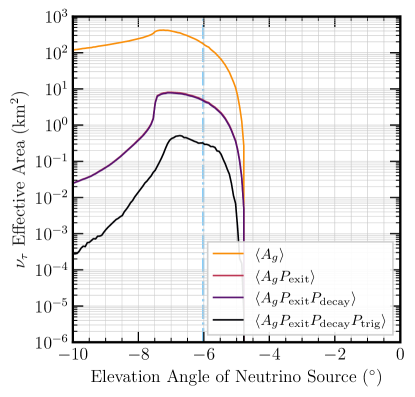
Figure 10: The effective area for $E_{\nu}=10$ EeV for an average location and position in the flight broken down into the various components that are calculated by tapioca as a function of the elevation angle of the neutrino source below ANITA’s horizontal. The dashed line indicates the approximate location of the geometric horizon in ANITA’s coordinate system.

IV Results

IV.1 Interpreting ANITA events as upgoing tau neutrinos

In §IV.1.1, we consider the observational evidence that the four near horizon events originated from upgoing $\tau$-neutrinos via the $\tau$-induced EAS channel. This includes considering the implied neutrino source directions, energies, and a spectral analysis against simulations. We find that the events are not inconsistent with the tau neutrino hypothesis. In §IV.2 and §IV.3, we further consider the implications of the tau neutrino hypothesis by considering both an isotropic, diffuse flux of tau neutrinos and point sources – both steady and transient – of tau neutrinos. This includes comparisons to other experimental searches for ultrahigh-energy tau neutrinos.

IV.1.1 Neutrino Source Parameters

Uncertainties in the location of the neutrino source on the sky with right-ascension ($\alpha$) and declination $(\delta)$ are dominated by the cone-shaped beam of the upgoing air shower radio emission, which itself varies with the $\tau$-lepton decay altitude and the zenith angle of the shower. This motivates the use of a forward modeling approach to reconstruct the location of the neutrino source and the corresponding energy of the neutrino that is most consistent with our observed events.

We developed a Markov Chain Monte Carlo simulation to reconstruct the posterior distributions of $(E_{\nu},\alpha,\delta)$; in particular, we use the emcee package [34] that implements an affine-invariant ensemble MCMC sampler [35]. For this reconstruction, we use the following likelihood function, implemented in tapioca, that captures the entire process of neutrino emission to the observed radio-frequency signal:

$$\mathcal{L}(E_{\nu},\alpha,\delta,t)\quad\propto\quad A_{g}\,P_{\mathrm{exit}}\,P_{\mathrm{decay}}\,\mathcal{L}_{\theta}\,\mathcal{L}_{\phi}\,\mathcal{L}_{\mathrm{waveform}}$$ (13)

where:

$A_{g}$ ${}={}$	the geometric area for a given $(\alpha,\delta,t_{\mathrm{event}},\vec{x}_{\mathrm{payload}})$,
$P_{\mathrm{exit}}$ ${}={}$	the probability that this neutrino generates a $\tau$-lepton that leaves the Earth,
$P_{\mathrm{decay}}$ ${}={}$	the probability that the $\tau$-lepton decayed before ANITA,
$\mathcal{L}_{\theta}$ ${}={}$	a Gaussian likelihood for the observed RF elevation angle,
$\mathcal{L}_{\phi}$ ${}={}$	a Gaussian likelihood for the observed RF azimuth angle,
$\mathcal{L}_{\mathrm{waveform}}$ ${}={}$	a sample-by-sample Gaussian likelihood for the residuals between the simulated waveform and the observed waveform.

Since the neutrino flux distribution at these energies is unobserved, we repeat this likelihood optimization for different priors on the neutrino spectrum. We assume a generic power law neutrino flux distribution, $E_{\nu}^{\gamma}$, between 0.1 EeV and 1000 EeV and reconstruct the neutrino parameters for discrete values $\gamma\in\left\{-3,-2,-1\right\}$ to accommodate a range of cosmogenic and astrophysical neutrino models.

We use broad ($6^{\circ}$ wide) uniform priors on $\alpha$ and $\delta$ centered around the sky location of the observed RF of each event. As an example, we consider the posterior distributions of $(E_{\nu},\alpha,\delta)$ for Event 72164985 (Figure 11). The most likely neutrino energy depends strongly on the assumed neutrino spectral index, $\gamma$. A harder spectra ($\gamma\sim-1$) is more likely to generate higher energy neutrinos that have more phase space for producing a decaying $\tau$ with sufficient shower energy to trigger ANITA; equivalently, a softer spectrum ($\gamma\sim-3$) strongly disfavors the production of higher energy $\nu_{\tau}$’s and therefore requires an upward fluctuation in the $\tau$ energy and shower fraction in order to be detected by ANITA. For $\gamma=-2$, the 50% quantile in reconstructed neutrino energy for Event 72164985 is $15.1$ EeV with lower and upper 1-$\sigma$ quantiles of $7.6$ EeV and $42.4$ EeV, respectively.

We note that the energies given in Table I of [1] are generic cosmic-ray shower energies (not neutrino energies) that were estimated using standard cosmic-ray shower models as opposed to the dedicated upward $\tau$ EAS simulations used in this work.

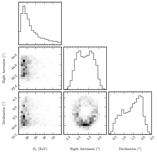
Figure 11: The posterior distributions of the neutrino energy and neutrino source locations, $(E_{\nu},\alpha,\delta)$, for Event 72164985 under a $\gamma=-2$ hypothesis as reconstructed by the emcee [36] Markov Chain Monte Carlo using the likelihood function in Equation 13. We note that the right-ascension and declination have been shifted by a random (constant) offset for this publication. The true reconstructed sky coordinates will be published in a follow-up paper by the ANITA collaboration.

The reconstructed neutrino parameters for all of the four events are shown in Table 2 under the various assumptions for $\gamma$. This MCMC, which forward models the entire process from incident neutrino to detection by ANITA, includes uncertainties in the detector models as described in §III.1, as well as the uncertainty in the observed event parameters.

Table 2: The most-likely reconstructed neutrino energies, using the MCMC approach described in § IV.1.1, for various priors on the neutrino flux.

Event	$E_{\nu,\gamma=-1}$ (EeV)	$E_{\nu,\gamma=-2}$ (EeV)	$E_{\nu,\gamma=-3}$ (EeV)
4098827	$49.8^{+80.3}_{-37.7}$	$12.5^{+29.9}_{-7.4}$	$5.2^{+6.0}_{-2.5}$
19848917	$31.9^{+76.0}_{-24.5}$	$5.2^{+11.0}_{-2.9}$	$2.6^{+3.1}_{-1.1}$
50549772	$45.4^{+83.4}_{-34.4}$	$8.8^{+19.5}_{-4.9}$	$4.3^{+4.8}_{-2.1}$
72164985	$60.3^{+88.9}_{-38.2}$	$15.1^{+27.3}_{-7.6}$	$8.9^{+10.5}_{-4.5}$

Since ANITA orbits the South Pole, ANITA’s elevation (azimuth) resolution is almost purely converted into declination (right-ascension) resolution. Figure 11 shows that the most likely neutrino source location $\alpha$ and $\delta$ is distributed as an annulus on the sky with an angular radius of $\sim 1^{\circ}$. This is due to the conically shaped radio emission from the EAS which has a Cherenkov angle of approximately $1^{\circ}$ in air.

Since ANITA only observes the radio emission at one point on the Cherenkov cone, the shower energy and the azimuthal angle around the shower axis (equivalently, which side of the cone you are observing) are degenerate as higher-energy showers may be observed with less radio power if the Askaryan and geomagnetic components are anti-aligned. Equivalently, if the Askaryan and geomagnetic components are aligned, this will result in an increase in the observed RF emission. It may be possible for ANITA to break this degeneracy through a detailed analysis of event polarization and the local geomagnetic field, but this is challenging to simulate due to the geometry of the near horizon events (see §V.2). The results of the MCMC shown in Figure 11 and Table 2 indicate that ANITA has approximately $\pm 1^{\circ}$ resolution in right-ascension and $\pm 0.5^{\circ}$ resolution in declination for the $\tau$-induced extensive air shower channel. We note that this is not ANITA’s resolution for reconstructing the observed direction of the RF emission (which is typically $\sim 0.2^{\circ}$, see [1]); the additional uncertainty is due to the uncertainty for the azimuthal angle around the shower axis of the EAS as well as the reconstruction of the off-axis angle of observation.

IV.1.2 Spectral Analysis

In this section, we compare the observed spectra against simulated spectra for upgoing $\tau$-induced EAS produced using ZHAireS [27]. The spectral shape of an upgoing air shower radio pulse can be approximated as a falling exponential above $\sim 300$ MHz [26, 25, 37]. The amplitude and exponential constant are dependent on the shower energy, the off-axis angle, the decay altitude of the $\tau$-lepton, and the zenith angle of the shower. The decay altitude and the zenith angle changes the atmospheric profile over which the shower develops, which affects the coherence of the radio emission, resulting in a different off-axis dependence as well as a lower required energy since the shower can develop closer to ANITA depending upon the decay length of the $\tau$ lepton.

Figure 12 shows the deconvolved electric field spectra for each event [1]. Since the spectrum of extensive air showers is well approximated by an exponential spectrum above 300 MHz, we also fit each deconvolved spectrum with an exponential function, $A(f)=A_{\mathrm{300}}\,e^{\gamma(f-300)}$, with $f$ in MHz where $\gamma$ is the spectral index. We also show a range of electric field spectra simulated by ZHAireS to demonstrate the range of spectral indices observed in upgoing $\tau$-induced air showers (light blue).

Event 72164985, which is closest to the horizon, is an excellent match to simulated upgoing EAS signals as well as the expected exponential spectral profile. Events 19848917 and 50549772 show a clear reduction in spectral power at low frequencies ($\lesssim 500~{}\mathrm{MHz}$). It is possible that atmospheric effects due to the long distance propagation from close to the horizon could create anomalous spectra like is seen in these events. Possible physical explanations for this missing low-frequency power are discussed in §V.1. For the purpose of our simulations, we do not include or model this low-frequency reduction and only fit the frequency range above the location of max spectral power (typically $300-500~{}\mathrm{MHz}$) for Events 19848917 and 50549772. Above $\sim 500$ MHz, the events appear to agree with our simulations as well as with the expected exponential shape.

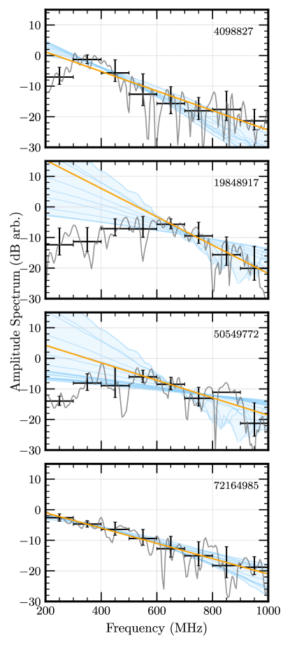
Figure 12: The deconvolved electric field amplitude spectrum for each event produced using the CLEAN deconvolution algorithm described in [1]. The amplitude spectrum (gray) is shown along with the average over consecutive independent 100 MHz bins (black). Each set of averages (black) was fit with an exponential form (orange), $A\exp(\gamma(f-300))$. For 4098827 and 72164985, the fit was performed from 300 MHz up to 1000 MHz. For 19848917 and 50549772, the fit was performed over the frequency region above the peak “turnover” (typically 500-600 MHz). Several different ZHAireS simulated upgoing $\tau$ spectra are also shown (light blue) for a variety of decay altitudes and zenith angles that could be consistent with these events.

We use tapioca to generate a sample of simulated $\tau$-EAS events that passed ANITA’s trigger so that we can compare these four events against the expected broader population of $\tau$ EAS. The spectral indices of each of the four near horizon events compared to the full population of normal (reflected and stratospheric) observed cosmic rays, as well as the simulated events, is shown in Figure 13. We do not necessarily expect that the spectral index of reflected UHECRs should match that of the simulated $\tau$-induced EASs due to the different event geometries as well effects from the reflection of the radio emission off the ice.

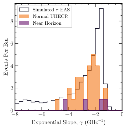
Figure 13: The exponential radio-frequency spectral slope distribution of the waveforms of the regular (reflected) cosmic rays (orange) observed by ANITA-IV compared against the spectral indices of the four near-horizon $\tau$-like events (purple) compared to an arbitrary scaled distribution of $\tau$ events simulated with tapioca. We note that to be consistent with previous ANITA publications, we have reused $\gamma$ here as the spectral slope (with units of inverse frequency) of the radio-frequency waveform whereas early (to be consistent with other published work) we also used $\gamma$ as the exponent in the power law neutrino flux distribution.

We perform a Kolmogorov-Smirnov (KS) test to determine whether the spectral indices of the four near horizon events are consistent with the underlying population of normal UHECRs or the simulated $\tau$ distributions. The results of this test are shown in Table 3.

Table 3: The results of a Kolmogorov-Smirnov test on the spectral index, $\gamma$, of the near horizon events compared against the sample of regular UHECRs and simulated $\tau$ EAS.

Test	p-value
Near horizon against regular UHECRs	0.48
Near horizon against simulated $\tau$ EAS (ZHaireS)	0.45

In both cases, the KS test finds no evidence that the four near horizon events are not drawn from the underlying distribution. The p-value of both cases is approximately 0.5 which is an order of magnitude worse than would be needed to reject the hypothesis that the four NH events came from each underlying distribution at a 5% significance.

Considering both the implied neutrino parameters $(E_{\nu},\alpha,\delta)$ and the spectral evidence, we conclude that these events are not inconsistent with $\tau$-induced EAS.

IV.2 Diffuse Flux Limits

Figure 14 shows the exposure of ANITA-IV to a diffuse $\nu_{\tau}$ flux via both the Askaryan [23] and upgoing EAS channels (this work). The upgoing EAS channel dominates ANITA’s $\nu_{\tau}$ exposure at energies below $\sim 10^{19}$ eV above which the Askaryan channel dominates. Due to the short flight of ANITA-IV ($\sim 28$ days), neither the Askaryan or EAS $\nu_{\tau}$ exposure is comparable with IceCube or Auger at energies below $\sim 10^{19.5}$ eV (the combined limit of ANITA I-IV sets a stronger limit than is shown in Figure 14). The significant discrepancy in the total exposure rules out a diffuse isotropic $\nu_{\tau}$ flux origin for the four ANITA-IV near horizon events under the Standard Model. This is the same conclusion reached for the two steeply upgoing events observed in ANITA-I and ANITA-III [5, 6] and consistent with the expected sensitivity of the three flights [9].

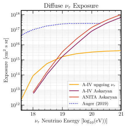
Figure 14: The (single-flavor) exposure to $\nu_{\tau}$ for ANITA’s EAS channel as well as its Askaryan in-ice detection channel [23] compared against $\nu_{\tau}$ exposures from the Pierre Auger Observatory [38].

IV.3 Point Sources

In this section, we present ANITA-IV’s sensitivity to astrophysical neutrino point sources, including transient sources that may have only been active for extremely short durations. Due to its unique viewing location in the stratosphere, ANITA typically has a large instantaneous effective area that partially compensates for its $\sim 30$ day observing time.

The effective area as a function of the elevation angle of the neutrino source on the sky for a range of energies from 1 EeV to 1000 EeV is shown in Figure 2. ANITA’s EAS sensitivity to $\nu_{\tau}$ turns on at several hundred PeV with a peak effective area of $\mathcal{O}$(1 km²) at the highest energies. By $\sim$300 EeV, ANITA’s effective area begins to saturate as the trigger probability tends to $\sim 1$ for events at these energies. ANITA’s peak sensitivity to neutrino sources occurs when the neutrino source is roughly $\sim 1^{\circ}$ below the horizon since this allows for a larger geometric area of possible neutrino exit locations for neutrinos from that source to be geometrically visible by ANITA and observed close to the Cherenkov angle (Figure 10 and Figure 2).

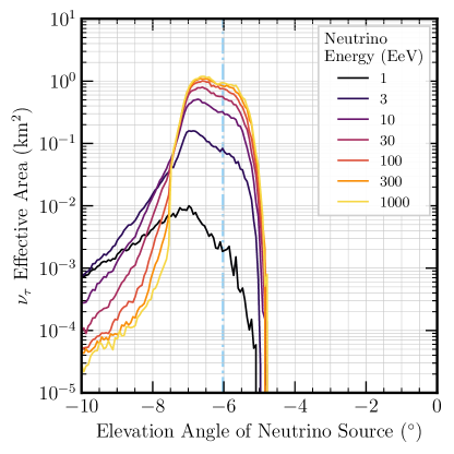
Figure 15: The effective area vs. neutrino source elevation angle for various tau neutrino energies from 1 EeV to 1000 EeV. The dashed blue line shows the approximate location of the geometric horizon (averaged over the flight).

The peak effective area of ANITA-IV as a function of incident neutrino energy for both the Askaryan channel (single-flavor effective area assuming a 1:1:1 flavor ratio) and the $\tau$ air shower channel is shown in Fig. 16. The effective area in the $\nu_{\tau}$ EAS channel exceeds that of the Askaryan channel, below $10^{19}$ eV and significantly lowers ANITA’s threshold energy for $\nu_{\tau}$ detection down to $\sim 0.3$ EeV. The sensitivity of the Askaryan channel exceeds the $\nu_{\tau}$ EAS channel above $10^{19}$ eV and can approach $\sim 30$ km² at the highest energies. We also show the Pierre Auger Observatory’s upgoing $\nu_{\tau}$ effective area over the same energy range using the published data from [10].

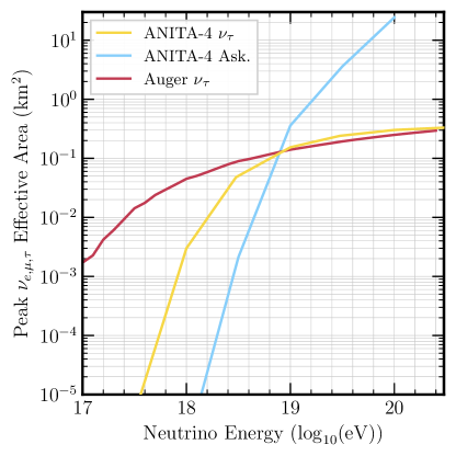
Figure 16: The peak all-flavor (1:1:1) effective area (over elevation angle) as a function of neutrino energy for the ANITA-IV air shower channel, the ANITA-IV Askaryan channel, and the Pierre Auger Observatory’s upgoing $\nu_{\tau}$ channel. The Auger curve was extracted using published data in [10].

IV.3.1 Consistency with $\nu_{\tau}$

We compare where our four observed events occur within the expected distributions of the elevation angles of $\tau$-induced EAS events as simulated by tapioca. Using the parameters (payload location, time, ice thickness, etc.) at the time of each observed near horizon event, we generate a large random sample of simulated $\nu_{\tau}$ air shower events that would have been detected by ANITA by sampling the calculated effective area shown in Figure 2. We use the energy curve closest in energy to the reconstructed neutrino energies shown in Table 2 assuming a $E^{-2}$ prior on the neutrino flux energy spectrum.

Given this distribution of elevation angles, we perform a series of Kolmogorov-Smirnov tests to determine if the observed events are consistent with the simulated event distributions; the p-values for the KS tests are shown in Table 4.

Table 4: The p-value of a Kolmogorv-Smirnov test for rejecting the hypothesis that these events are drawn from the simulated distribution of events from tapioca.

Event	KS p-value
4098872	0.95
19848917	0.60
50594772	0.72
72164985	0.85
All Events	0.19

For each observed event, there is no evidence to reject the hypothesis that the observed events are taken from the simulated distribution of elevation angles of $\tau$-induced EAS events. Under the model presented in this work, all four events taken together are observed at elevation angles that are not inconsistent with $\tau$-induced EAS.

IV.3.2 Field of View

ANITA has a relatively narrow instantaneous field-of-view on the sky (a $\sim 1^{\circ}$ wide band in elevation angle) for which it has a large effective area, so the effective area over time for a given sky coordinate is not constant due to the orbital movement of the payload and the sidereal motion of the source on the sky. The ANITA payload typically completes several full orbits around the geographic south pole (i.e. $\phi\in[-180,+180]$) with a latitude that varies between $-90^{\circ}$ and $\lesssim-75^{\circ}$

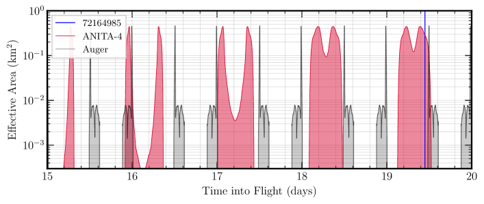
Figure 17: The time evolution of the effective area of ANITA-IV $\nu_{\tau}$ (pink) and Auger (grey) [10] in the direction of the peak source location corresponding to event 72164985 (see Table 2). Event 72164985 occurred at the time indicated by the blue line at day $\sim 19.5$. The Auger curves (simulated by us) were performed using the published curves in [10].

The instantaneous effective area at 1 EeV for a 5-day period encompassing the detection of Event 72164985 is shown in Figure 17 along with the effective area of the Pierre Auger Observatory [10]. As ANITA is also orbiting the continent, the shape and duration of each daily viewing period changes on a day-to-day basis. The time at which ANITA observed event 72164985 is shown with a blue vertical line. All four near horizon events were observed by ANITA during a window when they were not visible by Auger and occurred close to the daily peak in $\nu_{\tau}$ effective area.

As shown in Figure 17, ANITA’s effective area to a given neutrino source location on the sky can be large, but varies significantly as a function of time since the visible portion of the sky changes and ANITA’s effective area depends strongly on elevation angle. Therefore, ANITA can set different sensitivity limits on the point source flux depending upon the duration of the transient source. The instantaneous single event sensitivity (SES) limit set by ANITA-IV for short-duration ($<15$ minute) and long duration ($>1$ day) transient neutrino sources occurring at the location of the four observed near-horizon events is shown in Figure 18 (this SES limit is estimated using the method in [39]). Since each event was observed at a different location on the $A_{\mathrm{eff}}(\delta)$ curve, and since each of the sources moves in and out of ANITA’s field of view with different transit rates, the strength of the SES is different for each neutrino candidate location and for different event durations. However, since each event was observed very close to the peak in ANITA’s time-varying $\nu_{\tau}$ effective area, the short-duration SES limits for each event are similar

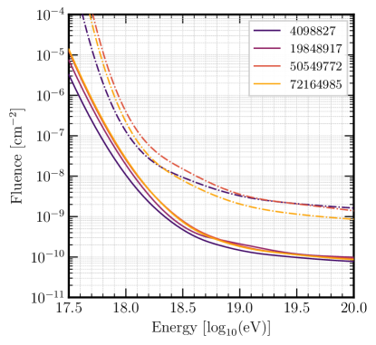
Figure 18: ANITA’s sensitivity to short-duration ($<15$ minute) (solid) and long duration ($>1$ day) (dashed) transient neutrino sources at the location of each of the four near-horizon events observed in ANITA-IV.

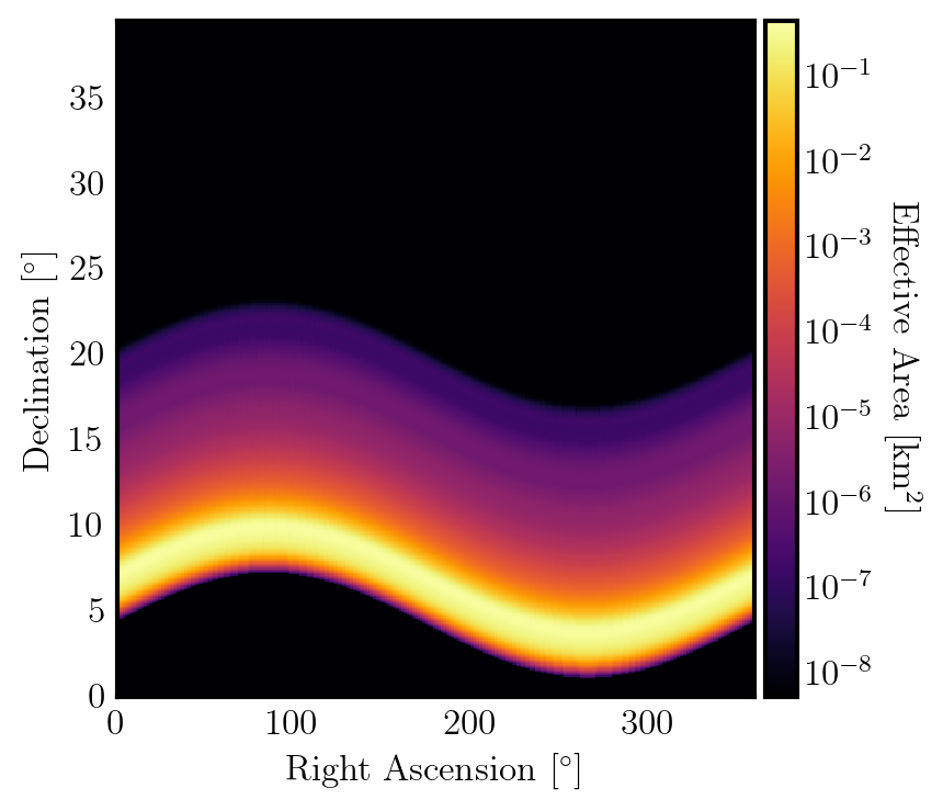
Figure 19: An instantaneous sky map of ANITA-IV’s $\nu_{\tau}$ effective area over right-ascension and declination at the time of observation of Event 72164985 for a neutrino energy of $100$ EeV.

IV.3.3 Comparison with other Observation Channels

Under the assumption that ANITA-IV observed 3-4 $\nu_{\tau}$ events (Figure 1) from a population of transient neutrino sources, we calculate the number of events that should have been observed by the Pierre Auger Observatory (Auger) as well as ANITA-IV’s Askaryan neutrino channel (which observed 1 candidate neutrino event consistent with background) [23].

The field of view (FoV) of ANITA’s $\nu_{\tau}$ EAS channel is compared to the ANITA Askaryan channel and Auger’s $\nu_{\tau}$ channel in Figure 20 and Figure 19. The FoV of both Earth-skimming $\nu_{\tau}$ channels (ANITA and Auger) are both $\sim 5^{\circ}$, as it is strongly driven by the exit probability of a $\tau$-lepton from a $\nu_{\tau}$ which is mostly independent of each detector. The peak effective area at 10 EeV is comparable for all three channels, with the Askaryan channel a factor of two higher than the two Earth-skimming ${\nu_{\tau}}$ channels.

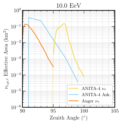
Figure 20: Single flavor effective area for the ANITA air shower channel (this work) and Askaryan channel [39] as well as the Auger Earth-skimming $\nu_{\tau}$ channel. The Auger curve was produced using published data from [10].

We compare ANITA and Auger’s sensitivity to a population of transient neutrino sources using a flux-model independent approach. We calculate the sensitivity of ANITA’s $\nu_{\tau}$ and Askaryan channels, as well as those of Auger, in logarithmic energy bins between 0.1 EeV and 1000 EeV. We then compare the fluence sensitivity for transients of various durations from 1 second to half-day timescales, as well as for different full-sky transient rates varying from 1 per-month to several thousand per day. While not an exhaustive search of the parameter space, this covers a representative sample of short- and long-duration transients that are potentially detectable by ANITA without detection by Auger. We simulate the period between May 1st, 2008 to August 31st, 2018 which corresponds to the published exposure and effective curves in [10]. This corresponds to a total of exposure time $T_{\mathrm{auger}}\sim 3700$ days during which ANITA-IV flew for 28 days starting in December 2016.

We use a dedicated Monte Carlo simulation to calculate the distribution of possible outcomes for the number of detected events for the ANITA $\nu_{\tau}$, ANITA Askaryan, and Auger channels. For a given transient duration $\Delta T$ and average full-sky event rate $r$, we throw $N\sim\mathrm{Poisson}(rT_{\mathrm{auger}})$ random sources on the sky throughout the $\sim 10$ years. For each source, we place a box-car (rectangular) time-dependent flux model at the time of each simulated event with the given transient duration, $\Delta T$. We then calculate the total integrated exposure to each of these transients using ANITA-IV’s $\nu_{\tau}$ effective area (this work), ANITA-IV’s Askaryan point source effective area [39], and Auger’s upgoing $\nu_{\tau}$ effective area [10]. While Auger has sensitivity to downgoing $\nu_{\tau}$ via in-air neutrino showers, this is significantly subdominant to the Earth-skimming $\nu_{\tau}$ channel and is therefore not included in this comparison. We calculate the total sensitivity across all sources visible by each experiment assuming that the underlying flux results in ANITA-IV observing $N_{\mathrm{true}}$ events, where $N_{\mathrm{true}}$ is sampled from Figure 1 and is typically $\sim 3$. Given $N_{\mathrm{true}}$ detections by ANITA-IV’s $\nu_{\tau}$ channel for this particular distribution of sources, we calculate corresponding limits on the fluence that would be set by ANITA-IV’s Askaryan channel and Auger assuming that no events were detected in either observatory. This process is a single realization of ANITA-IV/Auger in the Monte Carlo simulation. This is repeated many times ($N_{\mathrm{src}}\in\left[10^{5},10^{6}\right]$) to accurately sample the distribution of possible transient limits that each respective experiment may set. For a given underlying full-sky transient rate and duration, this Monte Carlo simulation accounts for fluctuations in the number and location of sources on the sky. The model independent limits on the fluence, calculated using this Monte Carlo, is shown in Figure 21 for two representative transient durations and rates.

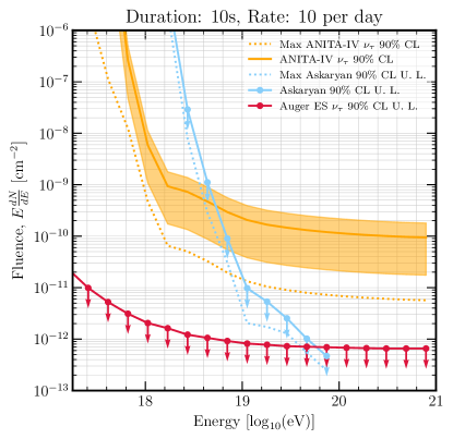
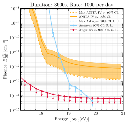
Figure 21: The fluence limits set by Auger $\nu_{\tau}$ and the ANITA-IV Askaryan channel assuming ANITA-IV observed $\sim 3$ $\nu_{\tau}$ events via the EAS channel. For both transient source duration and full-sky event rates simulated here, the range of $\nu_{\tau}$ fluences consistent with our observation (orange band) are inconsistent with the limits set by Auger (red curve) across the entire simulated energy range and inconsistent with ANITA-IV’s Askaryan limit (blue curve) above $\sim 10^{18}$ eV. All Auger results were calculated using the published effective areas from [10].

For all simulated transient durations and full-sky rates, the observation of $\sim 3$ $\nu_{\tau}$ events is in strong tension with Auger across the full simulated energy range, and is also in tension with ANITA-IV’s Askaryan channel above $\sim 10^{18.8}$ eV. This tension with ANITA’s Askaryan channel could potentially be resolved by a cut-off in the neutrino energy spectrum at or around $\sim 10^{19}$ eV but this would not eliminate the tension with Auger. As shown in Figure 20, ANITA-IV and Auger’s Earth-skimming $\nu_{\tau}$ channels have very similar instantaneous field-of-views so Auger immediately sets a stronger limit due to its $\sim 120\times$ longer livetime and larger effective area at lower energies (Figure 16). The strength of the fluence limit set by each detector can vary significantly with the transient duration and full-sky transient rate, but Auger always sets a stronger limit than the ANITA-IV $\nu_{\tau}$ channel by an approximately constant factor due to the similarity of each observatories’ fields-of-view and effective area. Above $10^{20}$ eV, ANITA-IV’s Askaryan channel is able to set a stronger limit (in $\sim 28$ days) than Auger for all simulated transient durations and full-sky transient rates.

V Discussion

The anomalous events found in ANITA-IV are significantly different from those found in the first and third flights in that they are closer to the horizon rather than being steeply upgoing. While this makes them more consistent with a Standard Model $\nu_{\tau}$ hypothesis as ANITA is maximally sensitive to $\nu_{\tau}$’s in the region below the horizon, the limits imposed by other observatories makes this an unlikely explanation. For an in-depth discussion of backgrounds associated with these events, including ice surface and subsurface features, coherent backscattering, stopping radiation, and other effects, see the appendix of [1].

In this section we briefly discuss the potential origin of the low-frequency spectral discrepancies observed in several of the anomalous events and speculate on future investigations related to these events.

V.1 Potential Origin for the Low-Frequency Attenuation

In Figure 12, we showed that while the spectra of events 4098827 and 72164985 match the expected exponential distribution, events 19848917 and 50549772 show attenuation at frequencies below $\sim 500$ MHz. We explore several possibilities for the origin of this low-frequency (LF) attenuation in two of the events: (1) geometries where ANITA simultaneously observes direct emission where an off-cone reflected emission whose inverted (from the reflection) waveform interferes with the direct pulse; and (2) atmospheric propagation effects, in particular tropospheric ducting, during the $\sim$600 km near-horizontal propagation of the electric field from the decay point to ANITA.

The “interfering” reflected hypothesis (1) can be further broken into two classes. In both classes, the direct radio signal from an Earth-skimming air shower is observed along with a reflected signal. While they both propagate close to the horizon, the two classes are distinguished by the particles that generate the air shower and their incoming angle. In class (a), a cosmic ray produces an elongated air shower above the horizon, in the stratosphere. In class (b), an upgoing $\tau$ lepton decay produces a skimming air shower originating from below the horizon. We consider both hypotheses by adding an inverted pulse – representing the reflected signal – to a non-inverted pulse – representing the direct signal. The inverted and non-inverted pulses are delayed and summed in the time-domain to match the observed time-domain waveforms.

To recreate the observed waveforms, the delay between the direct and reflected pulse must be less than $\sim$1 ns, or $\lesssim 30$ cm of total path length. An above-horizon cosmic ray geometry that allows for an off-axis reflection detectable by ANITA with a $\lesssim$30 cm path length must propagate extremely close to the ground and is therefore strongly suppressed by the near horizon radio propagation effects discussed in [40].

Furthermore, for each of the two events attenuated at low frequencies, the emergence angle at the Earth is $2^{\circ}-3^{\circ}$. For a $\tau$ energy of $\mathcal{O}(1-10\ \mathrm{EeV})$, the average $\tau$ lepton decay point is several kilometers above the ground (the decay length for a 1 EeV $\tau$ is 47 km). With a $\lesssim 30$ cm path length constraint, the relatively high-altitude of the $\tau$ decay rules out any possible geometry for a reflection.

The reflected signal must also be of similar strength to the direct pulse to create the observed waveforms shown in Fig.  12. As shown in [25], the total reflection coefficient including Fresnel, roughness, and curvature effects, approaches zero near the horizon significantly suppressing the strength of any reflection, further disfavoring any reflected explanation for the observed spectral attenuation below 250 MHz.

V.2 Limitations of simulations

The air shower simulation code used in this work, AIRES [41], makes several assumptions that may affect the simulation of near-horizontal cosmic ray showers from near-to or over-the horizon. In particular, AIRES, as well as the other major EAS simulation code CoREAS [42]: a) do not accurately simulate the curvature of the Earth and atmosphere at the 600 km scale of the ANITA events and therefore do not allow for “over the horizon” propagation; b) ignore the refraction of the radio emission from the shower during propagation to the receiving antennas; and c) use a geometric optics formalism that ignores any wave-like (diffraction, dispersion, ducting, etc.) effects that may occurs in real atmospheres and alter the propagation of the radio emission from the shower to the antenna. All of these effects are most dominant for events originating near the horizon (i.e. propagating close to the surface) where the Earth’s curvature is most significant and many wave-like effects are possible (i.e. tropospheric ducting, Fresnel zone attenuation or diffraction, etc.) which are often strongly frequency-dependent and could potentially explain the anomalous low-frequency spectra observed in two of these ANITA events.

The authors of ZHAireS have investigated the effect of ray curvature for highly-inclined reflected UHECR showers (as might be seen by ANITA) and found that for showers with zenith angles of $85^{\circ}$, the straight-ray approximation was valid up to $\sim 900$ MHz above which several changes in the angular spectrum could be observed [43]. The four events discussed in this work were observed at frequencies well below this frequency. Furthermore, the $\tau$-induced EAS events visible by ANITA are also less likely to be affected by these effects, compared to a high-zenith angle reflected EAS, since a $\tau$ lepton at these energies typically decays tens or hundreds of kilometers after leaving the Earth and therefore the shower typically develops far from the horizon and potentially several kilometers above the surface, away from the regions that are most affected by these approximations.

While this analysis has been performed using these existing tools as they are the best available at the time of writing, future efforts may help alleviate some (but not all) of these issues. The upcoming next-generation shower simulation tool CORSIKA 8 [44] allows for simulating showers in arbitrary 3D geometries so will allow for a correct treatment of Earth- and atmospheric curvature near the horizon. However, the current simulation programs of radio pulses in EAS based on superposition of contributions from particle sub-tracks (ZHS [45] and CoREAS [46]) do not currently account for the geometric refraction of rays during propagation. Future versions of these packages such as those planned to be implemented in CORSIKA 8 may be able to incorporate these effects and may significantly alter these results.

However, incorporating full-wave optic effects is a computationally challenging problem that will require the development of significantly new tools. The standard high-fidelity full-wave electromagnetics simulation tool is the finite-difference time-domain (FDTD) algorithm but this requires extremely large amounts of memory when simulating large volumes at high frequencies and simulating the propagation of ANITA’s near horizon events is currently computationally intractable on even the world’s largest supercomputers. Alternative methods, such as parabolic equation (PE) propagation, have the potential to provide more accurate wave-like simulations for EAS than current tools (ZHAireS, CoREAS) but are still computationally expensive and have so far primarily been developed for defense-related radar propagation and are only beginning to be employed for ultrahigh-energy neutrino physics [47].

V.3 Future Observations

Several current and future experiments are designed to search for upgoing tau neutrinos via the $\tau$-induced air shower channel. PUEO, the follow-up mission to ANITA, has significantly improved sensitivity to $\tau$-induced EAS events and includes dedicated hardware to improve analysis and reduce backgrounds [48]. Experiments searching for air showers from high elevation mountains [49, 50, 51, 52, 53], balloons [48], and satellites [54] are also sensitive to events with similar geometries and origins. Given that these events are challenging to interpret under a $\nu_{\tau}$ hypothesis, it will be important to follow-up the ANITA observations in different locations (overlooking water, rock,) and from different altitudes (mountain, balloon, satellite) that will have different systematics and backgrounds.

The point-like $\nu_{\tau}$ analysis by Auger used for this work also only includes the surface detectors. A tau search using Auger’s fluorescence detectors was also performed but only considered events with exit elevation angles greater than $20^{\circ}$ and so cannot be used to constrain these new ANITA-IV events [55, 56].

VI Conclusion

We have analyzed the plausibility that the upgoing near-horizon ANITA-IV events are explained by $\tau$-lepton extensive air showers from skimming $\nu_{\tau}$ interactions in the Earth. To achieve this, we have applied detailed models of the $\nu_{\tau}\to\tau$ propagation through the Earth, radio emission from air showers, and the ANITA-IV detector. We have found consistency in the elevation angles and radio-frequency impulsive signatures of these events, namely the polarity and spectral shape of the events, with reconstructed $\nu_{\tau}$ energies in the 1 - 50 EeV range (depending upon assumptions regarding the underlying neutrino flux shape). We find that while these events are not observationally inconsistent with UHE $\nu_{\tau}$’s, the implied fluence necessary for ANITA-IV to have observed $\sim 3$ of these events is in tension with Auger’s existing $\nu_{\tau}$ limits at all simulated energies and is also in tension with ANITA’s Askaryan channel above $10^{18.8}$ eV.