Stability in 3d of a sparse grad-div approximation of the Navier-Stokes equations

Abstract

Inclusion of a term $-\gamma\nabla\nabla\cdot u$, forcing $\nabla\cdot u$ to be pointwise small, is an effective tool for improving mass conservation in discretizations of incompressible flows. However, the added grad-div term couples all velocity components, decreases sparsity and increases the condition number in the linear systems that must be solved every time step. To address these three issues various sparse grad-div regularizations and a modular grad-div method have been developed. We develop and analyze herein a synthesis of a fully decoupled, parallel sparse grad-div method of Guermond and Minev with the modular grad-div method. Let $G^{\ast}=-diag(\partial_{x}^{2},\partial_{y}^{2},\partial_{z}^{2})$ denote the diagonal of $G=-\nabla\nabla\cdot$, and $\alpha\geq 0$ an adjustable parameter. The 2-step method considered is

$$1 :\frac{\widetilde{u}^{n+1}-u^{n}}{k}+u^{n}\cdot\nabla\widetilde{u}^{n+1}+\nabla p^{n+1}-\nu\Delta\widetilde{u}^{n+1}=f\text{ \& }\nabla\cdot\widetilde{u}^{n+1}=0,$$

$$2 :\left[\frac{1}{k}I+(\gamma+\alpha)G^{\ast}\right]u^{n+1}=\frac{1}{k}\widetilde{u}^{n+1}+\left[(\gamma+\alpha)G^{\ast}-\gamma G\right]u^{n}.$$

We prove its unconditional, nonlinear, long time stability in $3d$ for $\alpha\geq 0.5\gamma$. The analysis also establishes that the method controls the persistent size of $||\nabla\cdot u||$ in general and controls the transients in $||\nabla\cdot u||$ when $u(x,0)=0$ and $f(x,t)\neq 0$ provided $\alpha>0.5\gamma$. Consistent numerical tests are presented.

1 Introduction

We present and prove the long time, nonlinear stability of a fully uncoupled, modular, sparse grad-div (SGD) finite element methods (FEM), approximating the incompressible Navier-Stokes equations (NSE)

$$u_{t}+u\cdot\nabla u+\nabla p-\nu\Delta u=f(x,t)\text{ and }\nabla\cdot u=0.$$

The stability analysis also delineates how the method controls $||\nabla\cdot u||$. Sparse grad-div methods are one slice of research on improving mass conservation in finite element methods. The complementary slice, currently giving strong results, uses exactly divergence-free elements. These two, others and their interconnections are surveyed in [13]. The first sparse grad-div method considered herein is from Guermond and Minev [10], for which we sharpen their stability result. The second is a new but natural synthesis with the modular grad-div method of [8]. The flow domain $\Omega$ is a bounded open set in ${{{\mathbb{R}}}}^{3}$ with no slip boundary conditions $u=0$ on $\partial\Omega$ . Here $u\in{{{\mathbb{R}}}}^{3}$ is the velocity, $p\in{{{\mathbb{R}}}}$ is the pressure, $\nu$ is the kinematic viscosity, and $f\in{{{\mathbb{R}}}}^{3}$ is the external force. Let $\gamma$ denote the (preset) grad-div parameter. Following Olshanskii [18], the standard grad-div approximation (with a simple time discretization for concreteness) is the space discretization of

$$\frac{u^{n+1}-u^{n}}{k}+u^{n}\cdot\nabla u^{n+1}+\nabla p^{n+1}-\nu\Delta u^{n+1}-\gamma\nabla\nabla\cdot u^{n+1}=f(t^{n+1}),$$

$$\text{and}{{\text{ \ \ \ }}}\nabla\cdot u^{n+1}=0.$$ (1)

If (as here) neither the boundary conditions nor the viscosity depends on the fluid stresses, the added grad-div term is the only term coupling all velocity components. For $\gamma$ large, the condition number of the linear system increases [15]. Even for moderate $\gamma$, penalizing pointwise violation of incompressibility and asking $\nabla\cdot u$ to be orthogonal to the pressure space has been observed to cause solver issues [8]. To eliminate this coupling, reduce memory requirements, speed parallel solution and improve the robustness of iterative methods for the resulting linear system, several sparse grad-div methods have been devised. To specify the variant considered herein, let $G$ denote $-\nabla\nabla\cdot$ and $G^{\ast}$ to be the diagonal of $G$

$$G:=-\begin{bmatrix}\partial_{xx}&\partial_{xy}&\partial_{xz}\\ \partial_{yx}&\partial_{yy}&\partial_{yz}\\ \partial_{zx}&\partial_{zy}&\partial_{zz}\end{bmatrix}\text{ \& }G^{\ast}:=-\begin{bmatrix}\partial_{xx}&0&0\\ 0&\partial_{yy}&0\\ 0&0&\partial_{zz}\end{bmatrix}.$$

The synthesis of a sparse grad-div method of Guermond and Minev [10] with the modular grad-div method of [8] is as follows. Suppressing the space discretization, given $u^{n}$ two approximations, $\widetilde{u}^{n+1}$ and $u^{n+1}$, at the next time step are calculated by

$$1 :\frac{\widetilde{u}^{n+1}-u^{n}}{k}+u^{n}\cdot\nabla\widetilde{u}^{n+1}+\nabla p^{n+1}-\nu\Delta\widetilde{u}^{n+1}=f\text{ \& }\nabla\cdot\widetilde{u}^{n+1}=0,$$

$$and$$ (2)

$$2 :\left[\frac{1}{k}I+(\gamma+\alpha)G^{\ast}\right]u^{n+1}=\frac{1}{k}\widetilde{u}^{n+1}+\left[(\gamma+\alpha)G^{\ast}-\gamma G\right]u^{n}.$$

The linear solve in Step 2 uncouples into 3 smaller and constant in time systems (one for each velocity component). For example, the first sub-system, for the $x$ component of velocity, is

$$\left[I-k(\gamma+\alpha)\frac{\partial^{2}}{\partial x^{2}}\right]u_{1}^{n+1}=RHS_{1}\text{.}$$

With simple discretizations, structured meshes, mass lumping and axi-parallel domains the above $3$ sub-systems can even be written as one tridiagonal solve for the unknowns on each mesh line. The precise presentation, including the FEM discretization of their space derivatives, is given in Section 2. The condition number of the coefficient matrix of Step 2 is proven in the appendix (under typical assumptions for this estimation) to have a condition number that does not blow up as $\gamma+\alpha\rightarrow\infty$, but changes from parabolic conditioning to elliptic conditioning:

$$cond_{2}(A)\leq C\frac{h^{2}+k(\gamma+\alpha)}{1+k(\gamma+\alpha)}h^{-2}.$$

The usual $L^{2}(\Omega)$ norm is denoted $||\cdot||$. The following summarizes the essential result.

Theorem 1

Let $\gamma\geq 0$. The method (2) is unconditionally, nonlinearly, long time stable in $3d$ if $\alpha\geq 0.5\gamma$ and in $2d$ if $\alpha\geq 0$. Further, if $u^{0},\nabla u^{0}\in L^{2}(\Omega)$ and $||f(t^{n})||\leq C<\infty$ and $\alpha>0.5\gamma$ we have $\nabla\cdot u^{n}\rightarrow 0$ as $\gamma\rightarrow\infty$ in time-average

$$\lim\sup_{N\rightarrow\infty}\frac{1}{N}\sum_{n=1}^{N}||\nabla\cdot u^{n}||^{2}\leq C\gamma^{-1}.$$

If $u^{0}=0$, then for all $N$

$$\frac{1}{N}\sum_{n=0}^{N}||\nabla\cdot u^{n}||^{2}\leq C\gamma^{-1}.$$

1.1 Related work

It has been recognized for a while now that the usual velocity-pressure FEM can result in $\mathcal{O}(1)$ errors in mass conservation, $||\nabla\cdot u||=\mathcal{O}(1)$, e.g., John, Linke, Merdon and Neilan [13] and Belenli, Rebholz and Tone [1]. This $||\nabla\cdot u||=\mathcal{O}(1)$ is clearly evident in the $\gamma=\alpha=0$ tests in Section 5. The cure for this is added grad-div stabilization, a simple idea with strong positive consequences. Its origin seems to be in SUPG type local residual stabilization methods, Brooks and Hughes [4], and the idea of adding an operator positive definite on the constraint set in optimization. Detailed analysis of the discretization, including an added grad-div term, can be found in papers including Case, Ervin, Linke and Rebholz [5], Olshanskii and Reusken [20], Olshanskii [18], Jenkins, John, Linke and Rebholz [12], Braack, Bürman, John and Lube [3], Layton, Manica, Neda, Olshanskii and Rebholz [14], Galvin, Linke, Rebholz and Wilson [9] and Connors, Jenkins and Rebholz [6]. Preselection of the grad-div parameter $\gamma$ is treated in many places such as Heavner [11] and self-adaptive selection recently in Xie [23].

Linke and Rebholz [16] developed the first sparse grad-div method. Their method contributes no consistency error. It improves solver performance [2], [16], reducing coupling (in $3d$) from 3 components to 2 components followed sequentially by a 1 component solve. Since Linke and Rebholz achieve this with a modified pressure, stability in $3d$ is automatic, and higher-order time stepping is also available. Subsequent sparse grad-div methods of Guermond and Minev [10] achieved greater uncoupling at the expense of increased consistency error and reduced options for time stepping. Let $G$ denote $-\nabla\nabla\cdot$. Their first method selected $G^{\ast}$ to be the upper triangular part of $G$ and lagged the remainder: $\nabla\cdot u^{n+1}=0$ and

$$\frac{u^{n+1}-u^{n}}{k}+u^{n}\cdot\nabla u^{n+1}+\nabla p^{n+1}-\nu\Delta u^{n+1}+$$

$$\gamma G^{\ast}u^{n+1}-\gamma[G^{\ast}-G]u^{n}=f(t^{n+1}).$$

This method, sequentially uncoupling velocity components, was proved stable in $2d$ and observed but not proven stable in $3d$. Their second sparse grad-div method, equation (3.8) Section 3.3, uncoupled velocity components in parallel as follows. For $\alpha$ a free parameter select $G^{\ast}$ to be the diagonal of $G.$ The second method of Guermond and Minev [10] is $\nabla\cdot u^{n+1}=0$ and

$$\frac{u^{n+1}-u^{n}}{k}+u^{n}\cdot\nabla u^{n+1}+\nabla p^{n+1}-\nu\Delta u^{n+1}+$$

$$(\gamma+\alpha)G^{\ast}u^{n+1}-\left[(\gamma+\alpha)G^{\ast}-\gamma G\right]u^{n}=f(t^{n+1}).$$ (3)

In Theorem 3.3 they prove stability in $3d$ for $\alpha\geq 2\gamma.$ The proof given in Section 2 for the modular sparse grad-div method yields the following sharpening of their stability result.

Theorem 2

Under the same conditions as Theorem 1, the conclusions of Theorem 1 for method (2) hold as well for method (3).

Modular (non-sparse) grad-div was introduced in [8], where compared to standard grad-div methods, dramatic reductions in run times and increases in robustness were observed. Similar ideas for the grad-div operator were developed in Minev and Vabishchevich [17]. Finding $\mathcal{O}(k^{2})$ extensions of (SparseGD) with the same unconditional stability is nontrivial. The only step we are aware of (aside from defect/deferred corrections wrapped around the first-order approximation used by Guermond and Minev [10]) is Trenchea[22].

2 Analysis of modular sparse grad-div

This section makes the method and result precise and proves stability for $\alpha\geq 0.5\gamma$ and control of $\nabla\cdot u$ for $\alpha>0.5\gamma$ for the modular sparse grad-div algorithm. This work builds on Guermond and Minev [10], the work on modular grad-div in [8] and Rong and Fiordilino [21], and the numerical tests of a related method in Demir and Kaya [7]. We suppress the traditional sub- or super-scripts ”$h$” in finite element formulations. Let $(X,Q)\subset\left(\mathring{H}^{1}(\Omega)^{3},L_{0}^{2}(\Omega)\right)$ denote conforming, div-stable FEM velocity-pressure spaces. To simplify the notation, define the following bilinear forms and semi-norms.

Definition 3

In $3d$ (with the obvious modification for $2d$), define the symmetric bilinear forms

$$\begin{array}[c]{ccc}\mathcal{A}(u,v)&:=&(\gamma+\alpha)\left[\left(u_{1,x},v_{1,x}\right)+\left(u_{2,y},v_{2,y}\right)+\left(u_{3,z},v_{3,z}\right)\right],\\ \mathcal{B}(u,v)&:=&\mathcal{A}(u,v)-\gamma(\nabla\cdot u,\nabla\cdot v),\\ \mathcal{B}^{\ast}(u,v)&:=&\mathcal{B}(u,v)-\frac{1}{3}(\alpha-2\gamma)(\nabla\cdot u,\nabla\cdot v).\end{array}$$

If $a(u,v)$ is a symmetric, positive semi-definite bilinear form on $X$ we denote its induced semi-norm by $||v||_{a}^{2}=a(v,v).$

The nonlinear term below has been explicitly skew-symmetrized and treated linearly implicitly below. Other choices are possible within the analysis we present, such as the EMAC formulation [19].

Algorithm 4

[Modular SGD]Given the initial velocity $u^{0}$ and grad-div parameter $\gamma>0$, choose $\alpha\geq 0$.

Step 1: Given $u^{n}\in X$, find $(\tilde{u}^{n+1},p^{n+1})\in(X,Q)$, for all $(v,q)\in(X,Q)$ satisfying:

$$\left(\frac{\tilde{u}^{n+1}-{\ u}^{n}}{k},v\right)+\frac{1}{2}{\ }\left({u}^{n}\cdot\nabla\tilde{u}^{n+1},v\right)-\frac{1}{2}{\ }\left({u}^{n}\cdot\nabla v,\tilde{u}^{n+1}\right)$$

$$+\nu\left(\nabla\tilde{u}^{n+1},\nabla v\right)-\left(p^{n+1},\nabla\cdot v\right)=\left(f^{n+1},v\right),$$

$$\text{and }\left(\nabla\cdot\tilde{u}^{n+1},q\right)=0.$$

Step 2: Given $\tilde{u}^{n+1}\in X$, find $u^{n+1}\in X$, for all $v\in X$ satisfying:

$$(u^{n+1},v)+k\mathcal{A}(u^{n+1},v)=(\tilde{u}^{n+1},v_{h})+k\mathcal{B}(u^{n},v).$$

Step 1 uses the standard implicit method to calculate $\tilde{u}^{n+1}$ at $t=t^{n+1}$. Step 2 adds the sparse grad-div stabilization term to $\tilde{u}^{n+1}$ to get $u^{n+1}$. This separation of velocity approximations to one where $\nabla\cdot u{\Large\bot}Q$ and one where $||\nabla\cdot u||$ is small may be a reason for the increased robustness observed in [8]. For all time steps, the uncoupled, same block diagonal matrix $I+k(\gamma+\alpha)G^{\ast}$ arises in Step 2.

We begin with a lemma.

Lemma 5

Let $\gamma>0,\alpha\geq 0$, then

$$\mathcal{B}(v,v)\geq\frac{\alpha-2\gamma}{3}||\nabla\cdot v||^{2}.$$

Thus, if $\alpha\geq 2\gamma>0$ then $\mathcal{B}(v,v)\geq 0$ for all $v\in X$.
Otherwise, if $\alpha\geq 0$ then, for all $v\in X,$

$$\mathcal{B}^{\ast}(v,v)=\mathcal{B}(v,v)-\frac{1}{3}(\alpha-2\gamma)||\nabla\cdot v||^{2}\geq 0.$$ (4)

Proof. The second and third claim follow from the first. For the first, since $||\nabla\cdot v||^{2}=||v_{1,x}+v_{2,y}+v_{3,z}|||^{2}$ $\leq 3||v_{1,x}||^{2}+3||v_{2,y}||^{2}+3||v_{3,z}||^{2}$, we have

$$\mathcal{B}(v,v) =(\gamma+\alpha)\left[||v_{1,x}||^{2}+||v_{2,y}||^{2}+||v_{3,z}||^{2}\right]-\gamma||\nabla\cdot v||^{2}$$

$$=(\gamma+\alpha)\left[||v_{1,x}||^{2}+||v_{2,y}||^{2}+||v_{3,z}||^{2}\right]-\frac{\gamma+\alpha}{3}||\nabla\cdot v||^{2}$$

$$-\left[\gamma-\frac{\gamma+\alpha}{3}\right]||\nabla\cdot v||^{2}$$

$$\geq(\gamma+\alpha)\left[||v_{1,x}||^{2}+||v_{2,y}||^{2}+||v_{3,z}||^{2}\right]-$$

$$\frac{\gamma+\alpha}{3}\left[3||v_{1,x}||^{2}+3||v_{2,y}||^{2}+3||v_{3,z}||^{2}\right]+\left[\frac{\alpha-2\gamma}{3}\right]||\nabla\cdot v||^{2}$$

$$\geq\frac{\alpha-2\gamma}{3}||\nabla\cdot v||^{2}\geq 0.$$

 

For all cases in the following theorem, the stability is proven via a formula like

$$E^{n+1}-E^{n}+2kD^{n+1}\leq 2k(f,\widetilde{u}^{n+1}),$$

which immediately implies stability (by summing over $n=1,N$) provided the dissipation $D\geq 0$ and the energy $E$ is square of a norm of $u$. The $2d$ result and the one below for $\alpha\geq 2\gamma$ in $3d$ are noted by Guermond and Minev [10] for method (3).

Proposition 6

Consider the modular sparse grad-div method.

2d case: Assume $\gamma\geq 0$. In $2d$ it is unconditional stable when $\alpha\geq 0$:

$$\ \left[||u^{n+1}||^{2}+k\gamma(||u_{1,x}^{n+1}||^{2}+||u_{2,y}^{n+1}||^{2}\right]$$

$$-\left[\|u^{n}\|^{2}+k\gamma(||u_{1,x}^{n}||^{2}+||u_{2,y}^{n}||^{2}\right]+$$

$$\|\tilde{u}^{n+1}-u^{n}\|^{2}+||u^{n+1}-\tilde{u}^{n+1}||^{2}+2k\nu\|\nabla\tilde{u}^{n+1}\|^{2}\leq 2k(f^{n+1},\tilde{u}^{n+1}).$$

3d case: Suppose $2\gamma>\alpha\geq 0.5\gamma$, then in $3d$ it is unconditionally stable. It satisfies

$$E^{n+1}-E^{n}+2kD^{n+1}=2k(f,\widetilde{u}^{n+1}),$$

where

$$E^{n+1} =||u^{n+1}||^{2}+2k\left[\frac{1}{2}||u^{n+1}||_{\mathcal{B}^{\ast}}^{2}+\frac{2\gamma-\alpha}{6}||\nabla\cdot u^{n+1}||^{2}\right],$$

$$D^{n+1} =\nu\|\nabla\tilde{u}^{n+1}\|^{2}+\frac{1}{2k}\left[\|\tilde{u}^{n+1}-u^{n}\|^{2}+||u^{n+1}-\tilde{u}^{n+1}||^{2}\right]$$

$$+\frac{1}{2}||u^{n+1}-u^{n}||_{\mathcal{B}^{\ast}}^{2}+\frac{2}{3}\left(\alpha-0.5\gamma\right)||\nabla\cdot u^{n+1}||^{2}$$

$$+\frac{2\gamma-\alpha}{6}||\nabla\cdot(u^{n+1}+u^{n})||^{2}.$$

If $\alpha\geq 2\gamma$, then in $3d$ it is unconditionally stable. It satisfies

$$E^{n+1}-E^{n}+2kD^{n+1}=2k(f,\widetilde{u}^{n+1}),$$

where

$$E^{n+1} =||u^{n+1}||^{2}+k||u^{n+1}||_{\mathcal{B}}^{2},$$

$$D^{n+1} =\nu\|\nabla\tilde{u}^{n+1}\|^{2}+\frac{1}{2k}\left[\|\tilde{u}^{n+1}-u^{n}\|^{2}+||u^{n+1}-\tilde{u}^{n+1}||^{2}\right]$$

$$+\gamma||\nabla\cdot u^{n+1}||^{2}+\frac{1}{2}||u^{n+1}-u^{n}||_{\mathcal{B}}^{2}.$$

Control of $\nabla\cdot u$ in 3d: Suppose $\alpha>0.5\gamma$, $u^{0},\nabla u^{0}\in L^{2}(\Omega)$ and $||f(t^{n})||_{-1}\leq F<\infty$ . Then if $u^{0}=0$ we have for any $N$

$$\frac{1}{N}\sum_{n=1}^{N}||\nabla\cdot u^{n}||^{2}\leq C\gamma^{-1}.$$

For $u^{0}$ non-zero we have $\nabla\cdot u^{n}\rightarrow 0$ as $\gamma\rightarrow\infty$ in the discrete time averaged sense

$$\lim\sup_{N\rightarrow\infty}\frac{1}{N}\sum_{n=1}^{N}||\nabla\cdot u^{n}||^{2}\leq C\gamma^{-1}.$$ (5)

If $\alpha=0.5\gamma$ the above results hold with $||\nabla\cdot u^{n}||^{2}$ replaced by $||\nabla\cdot(u^{n+1}+u^{n})||^{2}$.

Proof. The 2d case: To shorten the $2d$ proof we set $\alpha=0$. The idea of the proof in $2d$ is simple. We perform a basic energy estimate and subsume the inconvenient terms in ones that fit the desired pattern. Set $v=\tilde{u}^{n+1}$, $q=p^{n+1}$ in Step 1. Use the polarization identity and multiply by $2k$. We obtain

$$\|\tilde{u}^{n+1}\|^{2}-\|u^{n}\|^{2}+\|\tilde{u}^{n+1}-u^{n}\|^{2}+2k\nu\|\nabla\tilde{u}^{n+1}\|^{2}=2k(f^{n+1},\tilde{u}^{n+1}).$$

Take $v=u^{n+1}$ in Step 2, use the polarization identity, multiply by $2$ and rearrange. We obtain

$$||u^{n+1}||^{2}-||\tilde{u}^{n+1}||^{2}+||u^{n+1}-\tilde{u}^{n+1}||^{2}+$$

$$2k\left\{\begin{array}[c]{c}\gamma(\nabla\cdot u^{n},\nabla\cdot u^{n+1})\\ +\gamma\left[(u_{1,x}^{n+1}-u_{1,x}^{n},u_{1,x}^{n+1})+(u_{2,y}^{n+1}-u_{2,y}^{n},u_{2,y}^{n+1})\right]\end{array}\right\}=0.$$

Add the last two equations. We obtain

$$||u^{n+1}||^{2}-\|u^{n}\|^{2}+\|\tilde{u}^{n+1}-u^{n}\|^{2}+||u^{n+1}-\tilde{u}^{n+1}||^{2}+2k\nu\|\nabla\tilde{u}^{n+1}\|^{2}$$

$$2k\left\{\gamma(\nabla\cdot u^{n},\nabla\cdot u^{n+1})+\gamma\left[(u_{1,x}^{n+1}-u_{1,x}^{n},u_{1,x}^{n+1})+(u_{2,y}^{n+1}-u_{2,y}^{n},u_{2,y}^{n+1})\right]\right\}$$ (6)

$$=2k(f^{n+1},\tilde{u}^{n+1}).$$

Expanding the term inside braces ($\{\cdot\}$) algebraically gives

$$\left\{\cdot\right\} =\gamma\left[||u_{1,x}^{n+1}||^{2}+||u_{2,y}^{n+1}||^{2}\right]-\gamma\left[(u_{1,x}^{n+1},u_{1,x}^{n})+(u_{2,y}^{n+1},u_{2,y}^{n})\right]$$

$$+\gamma(\nabla\cdot u^{n},\nabla\cdot u^{n+1})$$

$$=\gamma\left[||u_{1,x}^{n+1}||^{2}+||u_{2,y}^{n+1}||^{2}\right]+\gamma\left[(u_{2,y}^{n+1},u_{1,x}^{n})+(u_{1,x}^{n+1},u_{2,y}^{n})\right].$$

Using the Cauchy-Schwarz-Young inequality in the last line of the above, then yields

$$\left\{\cdot\right\}\geq\frac{\gamma}{2}\left[||u_{1,x}^{n+1}||^{2}+||u_{2,y}^{n+1}||^{2}\right]-\frac{\gamma}{2}\left[||u_{1,x}^{n}||^{2}+||u_{2,y}^{n}||^{2}\right].$$

Inserting this for the term in braces in (6) then implies

$$\left[||u^{n+1}||^{2}+k\gamma\left[||u_{1,x}^{n+1}||^{2}+||u_{2,y}^{n+1}||^{2}\right]\right]$$

$$-\left[\|u^{n}\|^{2}+k\gamma\left[||u_{1,x}^{n}||^{2}+||u_{2,y}^{n}||^{2}\right]\right]$$

$$+\|\tilde{u}^{n+1}-u^{n}\|^{2}+||u_{h}^{n+1}-\tilde{u}^{n+1}||^{2}+2k\nu\|\nabla\tilde{u}^{n+1}\|^{2}\leq 2k(f^{n+1},\tilde{u}^{n+1}).$$

Stability now follows by subsuming the $\tilde{u}^{n+1}$ on the RHS into $2k\nu\|\nabla\tilde{u}^{n+1}\|^{2}$ on the LHS and summing over $n$.

The 3d case: In $3d$ there are too many inconvenient terms to simply use the Cauchy-Schwarz-Young inequality as in $2d$ to establish the energy estimate. Set $v=\tilde{u}^{n+1}$, $q=p^{n+1}$ in Step 1, multiply by $2k$ and use the polarization identity to get

$$\left[\|\tilde{u}^{n+1}\|^{2}-\|u^{n}\|^{2}\right]+\|\tilde{u}^{n+1}-u^{n}\|^{2}+2k\nu\|\nabla\tilde{u}^{n+1}\|^{2}=2k(f^{n+1},\tilde{u}^{n+1}).$$ (7)

We note that Step 2 can be rewritten as

$$(u^{n+1},v)+k\gamma(\nabla\cdot u^{n+1},\nabla\cdot v)=(\tilde{u}^{n+1},v)-k\mathcal{B}(u^{n+1}-u^{n},v).$$

Take $v=u^{n+1}$ in this form of Step 2, use the polarization identity, multiply by $2$ and rearrange. We obtain

$$||u^{n+1}||^{2}-||\tilde{u}^{n+1}||^{2}+||u^{n+1}-\tilde{u}^{n+1}||^{2}+2k\gamma||\nabla\cdot u^{n+1}\mathbf{||}^{2}+$$

$$+2k\mathcal{B}(u^{n+1}-u^{n},u^{n+1})=0.$$ (8)

Add equation (7) and (8). We obtain

$$||u^{n+1}||^{2}-\|u^{n}\|^{2}+\|\tilde{u}^{n+1}-u^{n}\|^{2}+||u^{n+1}-\tilde{u}^{n+1}||^{2}+2k\nu\|\nabla\tilde{u}^{n+1}\|^{2}$$

$$+2k\left\{\gamma||\nabla\cdot u^{n+1}||^{2}+\mathcal{B}(u^{n+1}-u^{n},u^{n+1})\right\}=2k(f^{n+1},\tilde{u}^{n+1}).$$

3d case with $\alpha\geq 2\gamma$ . This case implies $\mathcal{B}(v,v)\geq 0$. Apply the polarization identity to the $\mathcal{B}-$semi-inner product and collect terms. This gives the following

$$\left[||u^{n+1}||^{2}+k||u^{n+1}||_{\mathcal{B}}^{2}\right]-\left[\|u^{n}\|^{2}+k||u^{n}||_{\mathcal{B}}^{2}\right]$$

$$+\|\tilde{u}^{n+1}-u^{n}\|^{2}+||u^{n+1}-\tilde{u}^{n+1}||^{2}+2k\nu\|\nabla\tilde{u}^{n+1}\|^{2}$$

$$+2k\left\{\gamma||\nabla\cdot u^{n+1}||^{2}+0.5||u^{n+1}-u^{n}||_{\mathcal{B}}^{2}\right\}=2k(f^{n+1},\tilde{u}^{n+1}).$$

Summing over $n=1,N$ yields stability when $\alpha\geq 2\gamma$.

3d case with $2\gamma>\alpha\geq 0.5\gamma$. We thus focus on the term in braces in the last equation. First, recall (4), $\mathcal{B}^{\ast}(v,v)\geq 0.$ Thus $\mathcal{B}^{\ast}$ induces a semi-norm $||\cdot||_{\mathcal{B}^{\ast}}$ to which a polarization identity can be applied. Motivated by this observation, rewrite algebraically the term in braces as

$$\left\{\gamma||\nabla\cdot u^{n+1}||^{2}+\mathcal{B}(u^{n+1}-u^{n},u^{n+1})\right\}=$$

$$=\left[\mathcal{B}(u^{n+1}-u^{n},u^{n+1})-\frac{\alpha-2\gamma}{3}(\nabla\cdot\left(u^{n+1}-u^{n}\right),\nabla\cdot u^{n+1})\right]+$$

$$+\left(\gamma||\nabla\cdot u^{n+1}||^{2}+\frac{\alpha-2\gamma}{3}(\nabla\cdot\left(u^{n+1}-u^{n}\right),\nabla\cdot u^{n+1})\right):=\left[I\right]+\left(II\right)$$

We expand and apply the polarization identity to the term in brackets, $\left[I\right]$, giving

$$\left[I\right] =\mathcal{B}^{\ast}(u^{n+1}-u^{n},u^{n+1})$$

$$=\frac{1}{2}\left(||u^{n+1}||_{\mathcal{B}^{\ast}}^{2}-||u^{n}||_{\mathcal{B}^{\ast}}^{2}+||u^{n+1}-u^{n}||_{\mathcal{B}^{\ast}}^{2}\right).$$

Recall that $2\gamma>\alpha\geq 0.5\gamma$, so that the multipliers are non-negative, $2\gamma-\alpha>0$ and $\alpha-0.5\gamma\geq 0$. The term in parentheses, $\left(II\right)$, is expanded as

$$\left(II\right)=\frac{\alpha+\gamma}{3}||\nabla\cdot u^{n+1}||^{2}+\frac{2\gamma-\alpha}{3}(\nabla\cdot u^{n},\nabla\cdot u^{n+1}).$$

Applying the polarization identity in the form $x\cdot y=-0.5(|x|^{2}+|y|^{2}-|x+y|^{2})$ to the term $(\nabla\cdot u^{n},\nabla\cdot u^{n+1})$ gives

$$\left(II\right) =\frac{\alpha+\gamma}{3}||\nabla\cdot u^{n+1}||^{2}-\frac{2\gamma-\alpha}{6}\left\{||\nabla\cdot u^{n+1}||^{2}+||\nabla\cdot u^{n}||^{2}\right\}$$

$$+\frac{2\gamma-\alpha}{6}||\nabla\cdot(u^{n+1}+u^{n})||^{2}.$$

This is rearranged algebraically to read

$$\left(II\right) =\frac{2\gamma-\alpha}{6}\left[||\nabla\cdot u^{n+1}||^{2}-||\nabla\cdot u^{n}||^{2}\right]+\frac{2}{3}\left(\alpha-0.5\gamma\right)||\nabla\cdot u^{n+1}||^{2}$$

$$+\frac{2\gamma-\alpha}{6}||\nabla\cdot(u^{n+1}+u^{n})||^{2}.$$

Putting all this together, we then have

$$E^{n+1}-E^{n}+2kD^{n+1}=2k(f,\widetilde{u}^{n+1}),$$

where

$$E^{n+1} =||u^{n+1}||^{2}+2k\left[\frac{1}{2}||u^{n+1}||_{\mathcal{B}^{\ast}}^{2}+\frac{2\gamma-\alpha}{6}||\nabla\cdot u^{n+1}||^{2}\right],$$

$$D^{n+1} =\nu\|\nabla\tilde{u}^{n+1}\|^{2}+\frac{1}{2k}\left[\|\tilde{u}^{n+1}-u^{n}\|^{2}+||u^{n+1}-\tilde{u}^{n+1}||^{2}\right]$$

$$+\frac{1}{2}||u^{n+1}-u^{n}||_{\mathcal{B}^{\ast}}^{2}+\frac{2}{3}\left(\alpha-0.5\gamma\right)||\nabla\cdot u^{n+1}||^{2}$$

$$+\frac{2\gamma-\alpha}{6}||\nabla\cdot(u^{n+1}+u^{n})||^{2}.$$

Since all terms are non-negative, stability follows by summing over $n$.

Control of $\nabla\cdot u$: The subtlety in concluding control of $||\nabla\cdot u||$ from stability is that $E^{0}$ & $D^{n}$ both depend on the grad-div parameter $\gamma$. For this reason we obtain control in a time averaged sense. Bound the RHS of the energy inequality by

$$2k(f,\widetilde{u}^{n+1})\leq k\nu||\nabla\tilde{u}^{n+1}\|^{2}+k\nu^{-1}F^{2}$$

and subsume the first term in $D$. This implies

$$E^{n+1}-E^{n}+kD^{n+1}\leq k\nu^{-1}F^{2}.$$

Summing this over $n=0,...,N-1$, dividing by $N$ and dropping the nonnegative $E^{N}$ term gives

$$k\frac{1}{N}\sum_{n=1}^{N}D^{n}\leq\frac{1}{N}E^{0}+k\nu^{-1}F^{2}.$$

The RHS is bounded uniformly in $N$ so the limit superior as $N\rightarrow\infty$ of the LHS exists. We thus have

$$\lim\sup_{N\rightarrow\infty}\frac{1}{N}\sum_{n=1}^{N}D^{n}\leq\nu^{-1}F^{2}\text{ }$$

and

$$\frac{1}{N}\sum_{n=1}^{N}D^{n}\leq\nu^{-1}F^{2}\text{ if }u^{0}=0.$$

The claimed result now follows since $D$ contains (with a positive multiplier) the term $\gamma||\nabla\cdot u^{n+1}||^{2}$ if $\alpha>0.5\gamma,$ and if $\alpha=0.5\gamma$ the term $||\nabla\cdot(u^{n+1}+u^{n})||^{2}$.   

3 Stability and control of $\nabla\cdot u$ for flow between 3d offset cylinders

We consider a $3d$ rotational flow obstructed by an offset cylindrical obstacle inside a cylinder. Let $r_{1}=1,r_{2}=0.1,(c_{1},c_{2})=(0.5,0)$ and

$$\Omega_{1}=\{(x,y):x^{2}+y^{2}<r_{1}^{2}\;\text{and}\;(x-c_{1})^{2}+(y-c_{2})^{2}>r_{2}^{2}\}.$$

The domain is $\Omega$ $=$ $\Omega_{1}\times(0,1)$, a cylinder of radius and height one with a cylindrical obstacle removed, depicted with the mesh used in Figure 1.

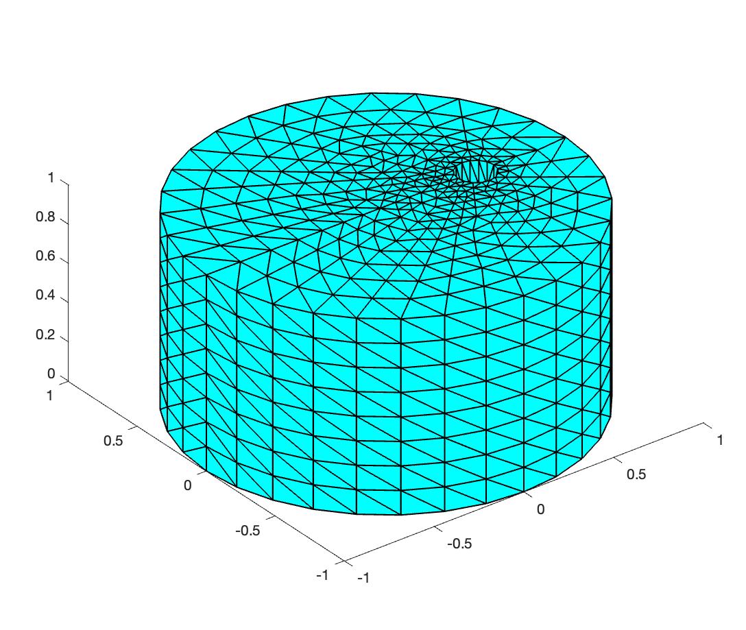
Figure 1: Mesh used to test stability

The flow is driven by a counter-clockwise rotational body force with $f=0$ on the outer cylinder

$$f(x,y,z,t)=\min\{t,1\}(-4y\ast(1-x^{2}-y^{2}),4x\ast(1-x^{2}-y^{2}),0)^{T},\;0\leq t\leq 10.$$

with no-slip boundary conditions, $u=0$, on boundaries. The space discretization uses $P^{2}-P^{1}$ Taylor-Hood elements with $18972$ total degrees of freedom in the velocity space and $2619$ total degrees of freedom in the pressure space. This mesh in Figure 1 is insufficient to test accuracy but suffices to test stability and control of $\nabla\cdot u$. The flow rotates about the $z-$axis and interacts with the inner cylinder. We start the test at rest, $u_{0}=(0,0,0)^{T}$, and choose the end time to be $T=10$. The kinematic viscosity is $\nu=0.0001$ and the time step is $\Delta t=0.05$.

We first tested if the extra $\alpha$ term is necessary for stability. We picked $\gamma=1.0,\alpha=0.5$ and $\alpha=0$ and $\gamma=\alpha=0$ (the method with no grad-div term), solved and plotted the kinetic energy and $||\nabla\cdot u||$ in Figure 2 below.

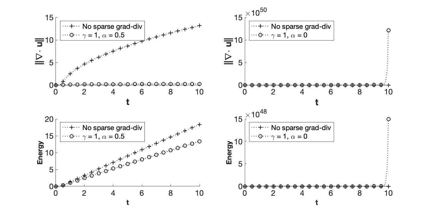
Figure 2: Modular SGD. The left two plots are stable $\gamma$ and $\alpha$ pair ($\gamma=1,\alpha=0.5$) compared with no sparse grad-div term. The right two are unstable $\gamma$ and $\alpha$ pair ($\gamma=1,\alpha=0$) compared with no sparse grad-div term.

The right hand side of the figure shows that the $\gamma=1.0,\alpha=0.0$ method is unstable while the $\gamma=1.0,\alpha=0.5$ is stable. This observed stability is consistent with the theoretical result.

The next question tested was whether $\alpha=0.5$ (for $\gamma=1$) is the critical value for stability. To test this, we choose $\gamma=1$ and the range of values $\alpha=0.3,0.4,0.48,0.49,0.5,0.6,0.7,1,2,3$, solved and plotted the kinetic energy and $||\nabla\cdot u||$ vs time in Figure 3 and Figure 4.

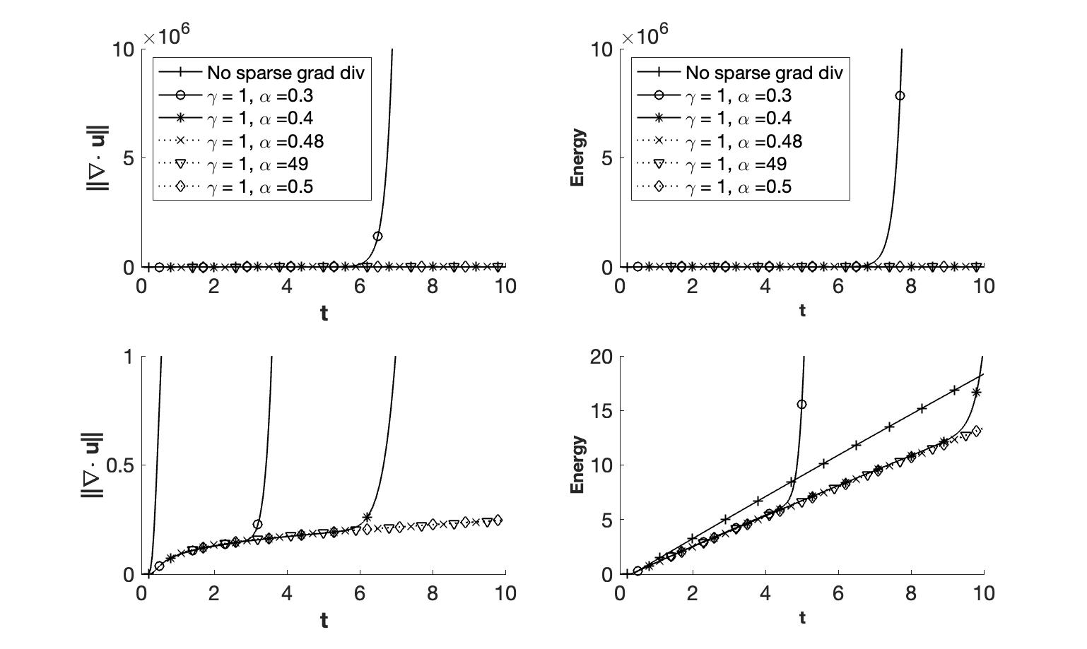
Figure 3: Testing the $\alpha\leq 0.5\gamma$, lower bound of $\alpha$ in (2). The left two plots are $\|\nabla\cdot u\|$ vs time. The right two plots are kinetic energy vs time. When $\alpha=0.3,0.4$, results show instability.

In Figure 4, method (2) is stable for $\alpha\geq 0.5$, and in Figure 3, for $\alpha<0.5$, the closer $\alpha$ is to the critical $0.5$ value, the longer time needed to see instability. No instability over $0<t<10$ was observed for the nearly critical values $\alpha=0.48$ & $0.49.$ This could be because the time interval $0<t<10$ was too short, because the derived value $\alpha=0.5$ is uniform in the viscosity $\nu$, so actual stability is slightly better than proven or because some sharpness was lost in the various inequalities. In further tests, we also observe $\alpha=0.45$ instability starts near $t=21.5$. Similar behavior was seen in the plots of $||\nabla\cdot u||$ in terms of control or loss of control of $\nabla\cdot u$. The only evidence in the plots of $||\nabla\cdot u||$ of non-sharpness of the analysis observed is that for $\alpha=0.5\gamma$, control of $||\nabla\cdot u||$ was observed. In contrast, the theorem predicted control of averages over $2$ time levels for $\alpha=0.5\gamma$. Please note that different scales were needed on the vertical axis.

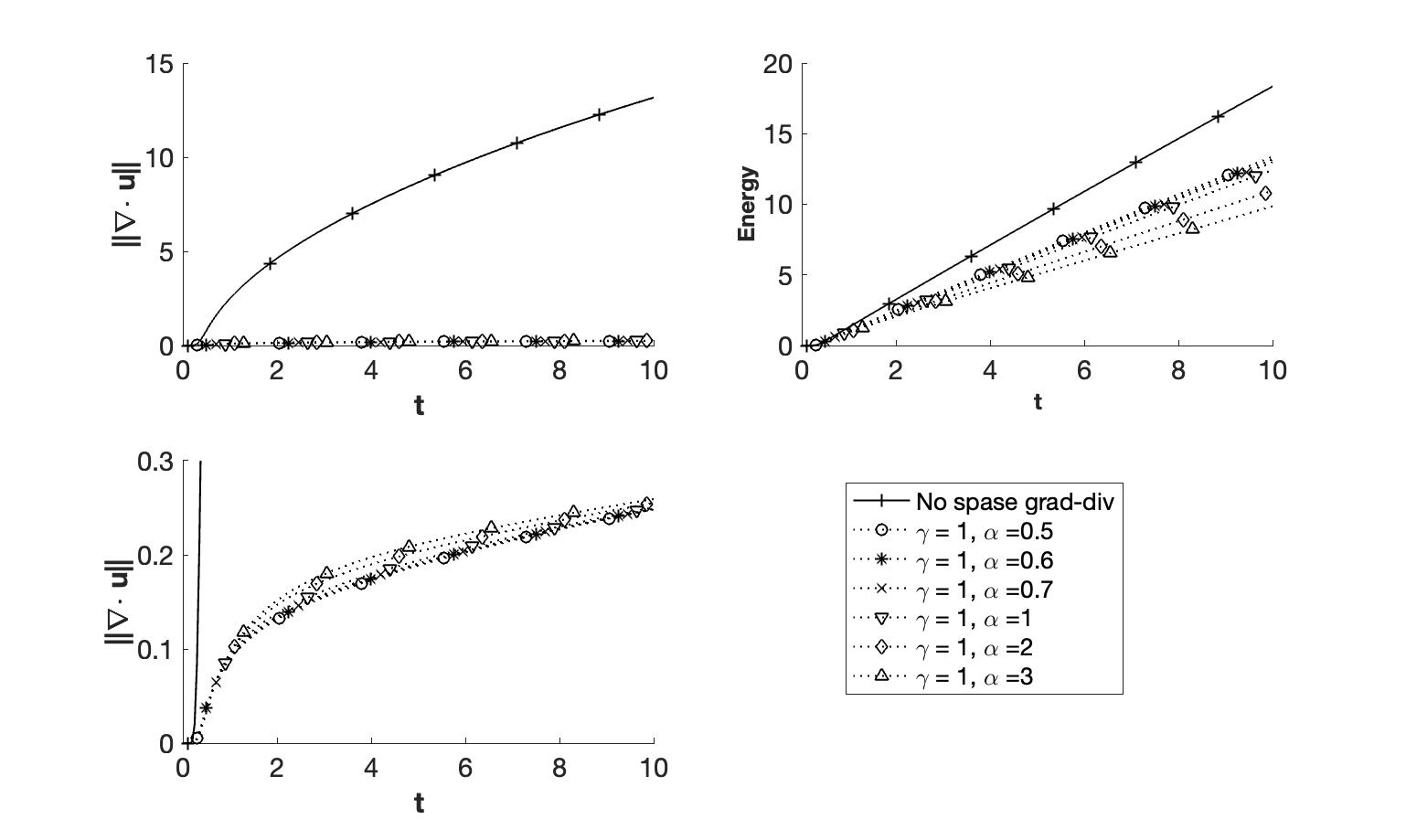
Figure 4: Testing the $\alpha\geq 0.5\gamma$, lower bound of $\alpha$ in (2). The left two plots are $\|\nabla\cdot u\|$ vs time. The right plot is kinetic energy vs time.

Next, we compare the effect of $\gamma$ in (2) on $||\nabla\cdot u||$. We choose $\gamma=0.1,1,10,20,50,100$ and $\alpha=0.5\ast\gamma$. For these values we solved and plotted the evolution of $||\nabla\cdot u||$ and kinetic energy in Figure 5.

The results in Figure 5 are consistent with $||\nabla\cdot u||$ decreasing as $\gamma$ increases. We also note that moderate values of $\gamma$, e.g. $\gamma=0.1$ and $10$, in this test seem to be effective. We conjecture that this is because $\nabla\cdot u=0$ is also required to be orthogonal to the pressure space. We also present the time-average $\|\nabla\cdot u\|^{2}$ and $\|\nabla\cdot u\|$ at end time $T=10$ for different $\gamma$ in Table.1. The convergence rate of average $\|\nabla\cdot u\|^{2}$ about $-1$ is consistent with our analysis in the control of $\nabla\cdot u$ in 3d.

We have also performed the above tests of (3). The results were similar so not detailed herein.

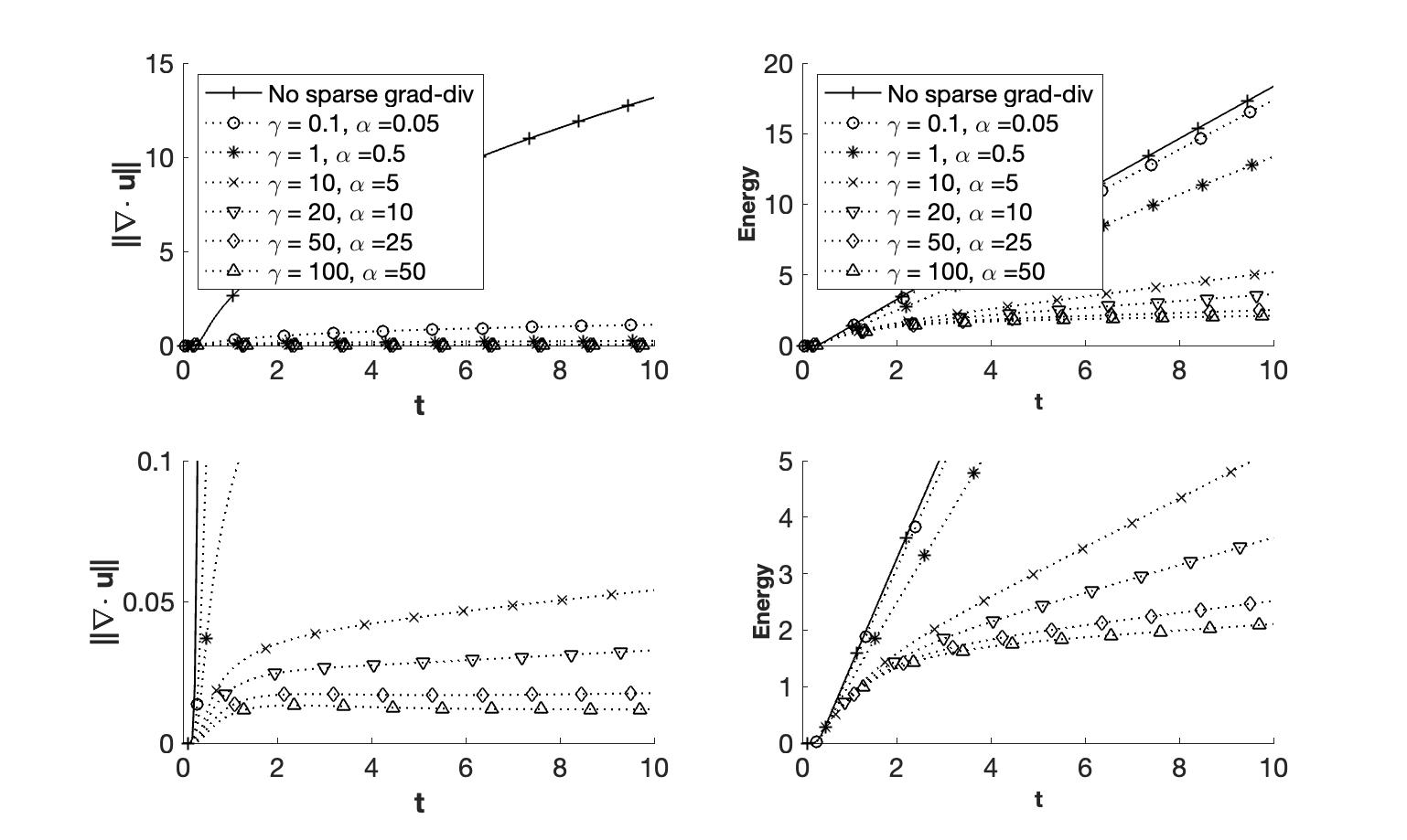
Figure 5: Effect of $\gamma$ in (2) on velocity and $\|\nabla\cdot u\|$. The left two plots are $\|\nabla\cdot u\|$ vs time. The right two plots are energy vs time.

$\gamma$	Avg($\|\nabla\cdot u\|^{2}$)	rate	$\|\nabla\cdot u(T)\|$	rate
0.1	0.64305	-	1.1033	-
1	0.033985	-1.28	0.24826	-0.65
10	0.0018455	-1.27	0.054152	-0.66
20	0.00074997	-1.30	0.032871	-0.72
50	0.00026663	-1.13	0.017703	-0.68
100	0.0001403	-0.93	0.01195	-0.57

Table 1: Time-average $\|\nabla\cdot u\|^{2}$ and $\|\nabla\cdot u\|$ at end time $T$ for different $\gamma$ value when $\alpha=0.5\gamma$.

4 Conclusions

With $\alpha\geq 0.5\gamma$ the algorithm presented is long time, nonlinearly stable in $3d$ and fully uncouples all velocity components in the associated linear system. For $\alpha<0.5\gamma$ the tests observed either instability or loss of control of $\nabla\cdot u$ (or both). The lower bound $0.5\gamma$ thus seems close enough to be sharp in the experiments to be useful. Open problems include providing an analysis of stability in $3d$ for the sparse grad-div method with $\alpha=0$ and $G^{\ast}$, the upper triangular part of $G$, and for higher-order time discretizations.

Acknowledgement 7

The research presented herein was supported by NSF grant DMS 2110379.

5 Appendix: condition number estimation

We give a brief analysis of the condition number of the coefficient matrix occurring in Step 2: Given $\tilde{u}^{n+1}\in X$, find $u^{n+1}\in X$, for all $v\in X$ satisfying:

$$(u^{n+1},v)+k\mathcal{A}(u^{n+1},v)=(\tilde{u}^{n+1},v_{h})+k\mathcal{B}(u^{n},v).$$

As noted in the introduction, the coefficient matrix is block diagonal with one block for each velocity  component. Since all blocks have similar structure and condition numbers, we estimate the condition number of the 1-1 block matrix. Let $\{\phi_{1},\cdot\cdot\cdot,\phi_{N}\}$ denote a standard finite element, nodal basis for the first component of the finite element space, denoted $X_{1}$. Then the 1-1 block matrix we consider is

$$A_{ij}=(\phi_{i},\phi_{j})+k(\gamma+\alpha)(\frac{\partial}{\partial x}\phi_{i},\frac{\partial}{\partial x}\phi_{j}),i,j=1,\cdot\cdot\cdot,N.$$

We assume the Poincaré-Friedrichs inequality holds in the x-direction, $A1$ (excluding x-periodic boundary conditions) and make the following 2 standard assumptions, $A2,A3$, on $X_{1}$. These have been proven for many spaces on quasi-uniform meshes.

A1 [Poincaré-Friedrichs]: For all $v\in X_{1},||v||\leq C||\frac{\partial v}{\partial x}||.$

A2 [Inverse estimates]: For all $v\in X_{1},||\nabla v||\leq Ch^{-1}||v||.$

A3 [Norm equivalence]: We have $N=Ch^{-d},d=\dim(\Omega)=2$ or $3.$ For all $v\in X_{1},v=\sum_{i=1}^{N}c_{i}\phi_{i}(x),||v||$ and $\sqrt{N^{-1}\sum_{i=1}^{N}c_{i}^{2}}$ are uniformly in $h$ equivalent norms.

For $|\cdot|$ the euclidean norm, we estimate $|A|$ and $|A^{-1}|$ below. These two estimates show that

$$cond_{2}(A)\leq C\frac{1+k(\gamma+\alpha)Ch^{-2}}{1+k(\gamma+\alpha)}.$$

For $|A^{-1}|$, let $Ac=b$ then $|A^{-1}|^{2}=\max_{b}|A^{-1}b|^{2}/|b|^{2}$. Let $M$ denote the finite element mass matrix $M_{ij}=(\phi_{i},\phi_{i})$. Solve $Ma=b$. Define

$$w=\sum_{i=1}^{N}c_{i}\phi_{i}(x),g=\sum_{i=1}^{N}a_{i}\phi_{i}(x).$$

Then $Ac=b$ implies $w,g$ satisfy

$$(w,v)+k(\gamma+\alpha)(\frac{\partial}{\partial x}w,\frac{\partial}{\partial x}v)=(g,v),\text{ for all }v\in X_{1}\text{.}$$

Setting $v=w$ and using A1 gives $\left(1+k(\gamma+\alpha)C^{2}\right)||w||\leq||g||$. Norm equivalence implies $||w||$ and $\sqrt{N^{-1}\sum_{i=1}^{N}c_{i}^{2}}$ are uniformly in $h$ equivalent norms. Norm equivalence applied twice implies $||w||$ and $\sqrt{N^{-1}\sum_{i=1}^{N}b_{i}^{2}}$ are uniformly in $h$ equivalent norms. Thus

$$|A^{-1}|\leq C\left(1+k(\gamma+\alpha)\right)^{-1}.$$

To estimate $|A|=\max_{c}|Ac|/|c|$, norm equivalence, A3, implies this is equivalent to estimating above $||g||/||w||.$ We have $||g||=\max_{v}(g,v)/||v||$. Then

$$\frac{(g,v)}{||v||} =\frac{(w,v)+k(\gamma+\alpha)(\frac{\partial w}{\partial x},\frac{\partial v}{\partial x})}{||v||}$$

$$\leq||w||+k(\gamma+\alpha)\frac{||\frac{\partial w}{\partial x}||||\frac{\partial v}{\partial x}||}{||v||}\text{ and by A2}$$

$$\leq||w||+k(\gamma+\alpha)Ch^{-2}||w||.$$

Thus, $||g||/||w||\leq 1+k(\gamma+\alpha)Ch^{-2}.$

References

[1]M.A. Belenli, L.G. Rebholz, and F. Tone, A note
on the importance of mass conservation in long-time stability of Navier-Stokes
simulations using finite elements, Applied Mathematics Letters, 45, 98-102, 2015
[2]A.L. Bowers, S. Le Borne and L.G. Rebholz,Error analysis and iterative solvers for Navier–Stokes projection
methods with standard and sparse grad-div stabilization. CMAME. 2014 Jun. 15;275:1-9.
[3]M. Braack, E.N. Bürman, V. John and G. Lube,
Stabilized finite element methods for the generalized Oseen problem.
CMAME 196(2007) 853–866.
[4]A.N. Brooks and T.J.R. Hughes, Streamline
upwind/Petrov-Galerkin formulations for convection dominated flows with
particular emphasis on the incompressible Navier-Stokes equations. CMAME.
1982 Sep 1;32(1-3):199-259.
[5]M.A. Case, V.J. Ervin, A. Linke and L.G. Rebholz,
A Connection Between Scott-Vogelius and Grad-Div Stabilized Taylor-Hood
FE Approximations of the Navier-Stokes Equations, SINUM, 49 (2011) 1461–1481
[6] J.M. Connors, E.W. Jenkins, and L.G. Rebholz,
On small-scale divergence penalization for incompressible flow problems
via time relaxation, I.J. Computer Math., 88(2011), 3202-3216.
[7]M. Demir and S., Kaya.A Numerical Study of a
Modular Sparse Grad-Div Stabilization Method for Boussinesq Equations. In
Journal of Physics: Conference Series 2019 Nov. 1 (Vol. 1391, No. 1, p. 012097).
[8]J.A. Fiordilino, W. Layton and Yao Rong.An
efficient and modular grad–div stabilization. CMAME. 2018 Jun. 15;335:327-46.
[9]K.J. Galvin, A. Linke, L.G. Rebholz and N.E. Wilson,
Stabilizing poor mass conservation in incompressible flow problems with
large irrotational forcing and application to thermal convection, CMAME, 237
(2012) 166–176.
[10]J.L. Guermond and P.D. Minev, High-order time
stepping for the Navier-Stokes equations with minimal computational
complexity, J. Comp. and Applied Mathematics, 310 (2017), pp. 92-103.
[11]N.D. Heavner, Locally chosen grad-div
stabilization parameters for finite element discretizations of incompressible
flow problems, SIURO, 7(2017) SO1278.
[12]E.W. Jenkins, V. John, A. Linke and L.G. Rebholz,
On the parameter choice in grad-div stabilization for the Stokes
equations, Advances in Computational Mathematics, 40 (2014) 491–516
[13]V. John, A. Linke, C. Merdon, M. Neilan, and L.G.
Rebholz,On the divergence constraint in mixed finite element methods
for incompressible flows, SIAM Review (2016).
[14]W. Layton, C.C. Manica, M. Neda, M. Olshanskii and
L.G. Rebholz,On the accuracy of the rotation form in simulations of
the Navier-Stokes equations, Journal of Computational Physics, 228 (2009) 3433–3447.
[15]A. Linke and C. Merdon, Pressure-robustness and
discrete Helmholtz projectors in mixed finite element methods for the
incompressible Navier–Stokes equations, CMAME, 311 (2016), 304–326.
[16]A. Linke and L.G. Rebholz, On a reduced sparsity
stabilization of grad–div type for incompressible flow problems. CMAME. 2013
Jul. 15;261:142-53.
[17]P. Minev and P.N. Vabishchevich, Splitting schemes
for unsteady problems involving the grad-div operator, Appl. Numer. Math.,
124 (2018), pp. 130-139
[18]M.A. Olshanskii, A low order Galerkin finite
element method for the Navier-Stokes equations of steady incompressible flow:
a stabilization issue and iterative methods. CMAME, 191 (2002) 5515–5536.
[19]M.A. Olshanskii and L.G. Rebholz, Longer time
accuracy for incompressible Navier–Stokes simulations with the EMAC
formulation. CMAME (2020) 1;372-113369.
[20]M.A. Olshanskii and A. Reusken, Grad-Div
stabilization for the Stokes equations. Math. Comp., 73(2004)1699–1718.
[21]Yao Rong and J.A. Fiordilino,Numerical Analysis
of a BDF2 Modular Grad–Div Stabilization Method for the Navier–Stokes
Equations. Journal of Scientific Computing. 2020 Mar;82(3):1-22.
[22]C. Trenchea, Second-order unconditionally stable
ImEx schemes: implicit for local effects and explicit for nonlocal effects.
ROMAI J. 12 (2016), no. 1, 163–178.
[23]Xihui Xie, On Adaptive Grad-Div Parameter
Selection. arXiv preprint arXiv:2108.01766. 2021 Aug 3.