Fiducial Inference and Decision Theory

Abstract

The majority of the statisticians concluded many decades ago that fiducial inference was nonsensical to them. Hannig et al. (2016) and others have, however, contributed to a renewed interest and focus. Fiducial inference is similar to Bayesian analysis, but without requiring a prior. The prior information is replaced by assuming a particular data generating equation. Berger (1985) explains that Bayesian analysis and statistical decision theory are in harmony. Taraldsen and Lindqvist (2013) show that fiducial theory and statistical decision theory also play well together. The purpose of this text is to explain and exemplify this together with recent mathematical results.

1 Introduction

The fiducial density $\pi(\rho\operatornamewithlimits{{\mid}}r)$ of the correlation $\rho$ given the empirical correlation $r$ is

$$\pi(\rho\operatornamewithlimits{{\mid}}r)=\frac{(1-r^{2})^{\frac{\nu-1}{2}}\cdot(1-\rho^{2})^{\frac{\nu-2}{2}}\cdot(1-r\rho)^{\frac{1-2\nu}{2}}}{\sqrt{2}B(\nu+\frac{1}{2},\frac{1}{2})}\cdot F(\frac{3}{2},-\frac{1}{2};\nu+\frac{1}{2};\frac{1+r\rho}{2})$$ (1)

where $B$ is the Beta function, $F$ is the Gaussian hypergeometric function, and $n=\nu-1$ is the sample size (Taraldsen, 2021a). The fiducial is also given by Rao’s formula

$$\pi(\rho\operatornamewithlimits{{\mid}}r)=\frac{(1-r^{2})^{\frac{\nu-1}{2}}\cdot(1-\rho^{2})^{\frac{\nu-2}{2}}}{\pi(\nu-2)!}\partial_{\rho r}^{\nu-2}\left\{\frac{\theta-\frac{1}{2}\sin 2\theta}{\sin^{3}\theta}\right\}$$ (2)

where $\cos\theta=-\rho r$ and $0<\theta<\pi$. Rao’s formula (2) is stated as the very last formula in the classical book Statistical Methods and Scientific Inference by Fisher (1956, eq.(234)). The fiducial for the correlation is also the very first example of a fiducial distribution presented by Fisher (1930).

It is no longer possible to ask Fisher in person, but from his writings it seems he would still claim:

The fiducial is the answer!

We agree. The problem Fisher gave us is then to explain and characterize relevant questions. This is a very open-ended problem, and it still needs more investigation. The original claim of the naturalness of the fiducial by Fisher (1930), and the many questions and more specific claims that followed have inspired the development of classical and Bayesian practical, theoretical, and mathematical statistics. It still does.

Recent mathematical results that give links between different modes of inference are presented in an Appendix here without any particular interpretation. Section 4 includes a brief discussion of related work, and comments on open problems. The majority of the text is devoted to exemplifying the interplay between fiducial arguments and decision theory as described by Taraldsen and Lindqvist (2013). Section 3 contains examples and Section 2 presents decision theory illustrated with a simple example. In the rest of this Introduction a direct interpretation of the fiducial distribution is explained.

Consider the following two equivalent equations

$$r=r(\rho,u)\iff\rho=\rho(r,u)$$ (3)

The first equation gives the uncertainty of the empirical correlation $r$ for a known correlation $\rho$ from the uncertainty in a Monte Carlo variable $u$. It is called a data generating equation since computer generated samples from $u$’s distribution gives samples from the distribution of $r$ when $\rho$ is known. A data generating equation $r=r(\rho,u)$ follows from a data generating equation for the binormal. It is not unique, but $\pi(\rho\operatornamewithlimits{{\mid}}r)$ is unique.

The second equality in equation (3) is equivalent with the first equality. It gives the uncertainty of the correlation $\rho$ for a known empirical correlation $r$ from the uncertainty in $u$. It is called a parameter generating equation since computer generated samples from $u$’s distribution gives samples from the distribution of $\rho$ when $r$ is known. The corresponding density of $\rho$ when $r$ is known is given by the two alternative expressions in equation (1) and equation (2) respectively. The fiducial distribution is hence simply the result of propagation of the uncertainty as defined by the uncertainty in $u$ and the generating equations (3).

The interpretation of the fiducial in a pure fiducial perspective is as the state of knowledge of the parameter $\rho$ given the data and the parameter generating model. This determines then also the state of knowledge of any derived parameter $\lambda=\lambda(\rho)$. This interpretation is exactly as for a Bayesian prior and for a Bayesian posterior, but it is to be used for cases without a prior. Taraldsen and Lindqvist (2019, p.523-4) explain and discuss this point in more detail. It is also this interpretation which is stated directly by Fisher (1956, p.54-5):

By contrast, the fiducial argument uses the observations only to change the logical status of the parameter from one in which nothing is known of it, and no probability statement about it can be made, to the status of a random variable having a well-defined distribution.

Consider an example where the result of an experiment is given by four points with $(x,y)$ coordinates $(773,727)$, $(777,735)$, $(284,286)$, and $(519,573)$ (Taraldsen, 2021a). There are reasons a priori for assuming a linear relationship. This is further supported by Figure 1, and a high value for the coefficient of determination $R^{2}=97.00\%$.

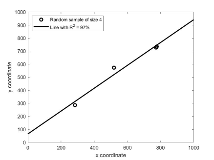
Figure 1: A regression line corresponding to an example by Fisher (1930, p.434).

The $R^{2}$ equals the square of the empirical correlation $r=98.49\%$. This is an example of linear regression used extensively in applied sciences.

A natural question is: What about uncertainty? In fiducial inference the uncertainty is given by the fiducial distribution. The state of knowledge regarding the correlation is given by the fiducial density shown in Figure 2.

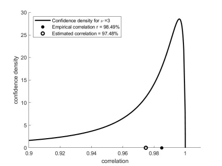
Figure 2: The fiducial density for correlation in the Fisher (1930, p.434) example.

The uncertainty of any derived parameter $\lambda(\rho)$ follows by propagation of uncertainty.

What about decision theory? In this case a natural question would be to find a point or interval esimate $\hat{\rho}$ for $\rho$. Decision theory gives one possible approach. A possible loss function for a point estimate is the absolute loss

$$l=\left|\hat{\rho}-\rho\right|$$ (4)

The fiducial risk

$$\int l(\hat{\rho},\rho)\pi(\rho\operatornamewithlimits{{\mid}}r)\,d\rho=\int\left|\hat{\rho}-\rho\right|\pi(\rho\operatornamewithlimits{{\mid}}r)\,d\rho$$ (5)

is minimized by the median $\hat{\rho}=97.48\%$. This is different from the ordinary estimate given directly by $r=98.49\%$.

The median is the optimal estimate given the particular loss in equation (4). In general, the loss depends on the particular application of the analysis. The absolute loss has the advantage of giving an estimate which is invariant under one-one transformations of the parameter.

2 Fiducial decision theory

Given data $y$ it is required to find an action $x=x(y)$ that is optimal. Optimality can be formalized starting with the specification of a loss

$$l=l(\gamma,x)$$ (6)

corresponding to a parameter $\gamma$ and the action $x$. An example for a real statistic is given by squared error loss

$$l=(\gamma-x)^{2}$$ (7)

The estimate $x$ can be a test, a set estimate, a distribution estimate, or more complicated objects, and then other loss functions are natural.

It will be assumed in this section that a fiducial distribution for $\gamma$ is given by the distribution of a random quantity $\Gamma^{y}$. An example was given in the Introduction and further examples will be given. A more general class of fiducial distributions are given by Definition 2 in the Appendix. This class of fiducial distributions includes all the examples in the following. The random quantity $\Gamma^{y}=\gamma(U^{a},y)$ is obtained by solving a data generating equation. The distribution of $U^{a}$ is the updated state of knowledge of $u$ given the data $y$. The value $a=a(y)$ is the observed value of a maximal invariant statistic $A=a(Y)$.

The distribution of the loss $l(\Gamma^{y},x(y))$ for each $y$ determines if an action $x$ is good. More generally, the joint distribution of $l(\Gamma^{y},x_{A}(y))$ and $l(\Gamma^{y},x_{B}(y))$ for each $y$ can be used in a comparison of two actions. The analysis can sometimes be simplified by only considering a simpler statistic given by a single number. The fiducial risk, if it exists, is defined to be the expected loss

$$r={\operatorname{\text{E}}}l(\Gamma^{y},x)$$ (8)

The fiducial risk of an action $x=x(y)$ is a statistic $r=r(y)$. An action $x^{*}$ is a best fiducial action if it’s fiducial risk $r^{*}$ is smaller than or equal to any other risk.

A best fiducial action $x=x(y)$ can in good cases be obtained directly by minimizing the risk. As a solution of an optimization problem a best fiducial action is also called an optimal fiducial action. The prototypical example is given by

$$x(y)={\operatorname{\text{E}}}\Gamma^{y}$$ (9)

which minimizes the risk from the squared error loss in equation (7). More generally, the optimization problem is much simplified both practically and theoretically if $x\mapsto l(\gamma,x)$ is convex for all $\gamma$.

An example is given by the maximum likelihood estimator $y$ of the scale $\theta>0$ from a random sample of size $n$ from a gamma distribution with known shape $\alpha>0$. The maximum likelihood estimator $y$ of $\theta$ equals the empirical mean of the sample and the law of $u$ is a gamma distribution with shape $n\alpha$ and scale $(n\alpha)^{-1}$. The model generating equation is $y=\theta u$ is given simply by multiplication. Taraldsen and Lindqvist (2015) investigate this and some related models in more detail.

Fiducial inference is in this simple case given by solving $y=\theta u$ with the result

$$\theta=yu^{-1}$$ (10)

The fiducial distribution is hence an inverse gamma distribution scaled by the data $y$. Exact simulation from this fiducial, and also the fiducial for any focus parameter $\gamma=\gamma(\theta)$, is obtained directly from the generator $u$.

In this case the maximal invariant is trivial (a constant), and the state of knowledge of $u$ is unchanged by the observation. Formally, in this case, $U^{a}\sim U$. The three examples in Section 3 demonstrates the more complicated case where the state of knowledge of $u$ is updated by the data and $U^{a}\not\sim U$.

For the loss in equation (7) for the gamma scale model the fiducial optimal action is

$$x={\operatorname{\text{E}}}\Theta^{y}=\left(\frac{n\alpha}{n\alpha-1}\right)y$$ (11)

assuming $n\alpha>1$. It can be observed that this estimate is different from the MLE $y$, but for large $n\alpha$ the difference is small.

Existence and calculation of a fiducial optimal action is hence similar to the problem of finding an optimal Bayesian posterior action. Berger (1985) and Eaton (1989) provide many examples and theory related to calculating optimal Bayesian actions. In addition to estimation this includes hypothesis testing and randomized actions.

The next aim is, as in textbooks on Bayesian decision theory, to provide a link to frequentist decision theory. The distribution of $l(\gamma,X)$ determines if the action $X=x(Y)$ is good. A data generating equation can be used to investigate this for each model $\theta$. This gives a method for comparison of two actions $X_{A}$ and $X_{B}$. Instead of a comparison of the distribution of $X_{A}$ and $X_{B}$ one should instead compare the distribution of the losses $l(\gamma,X_{A})$ and $l(\gamma,X_{B})$. It can be observed that a data generating model allows simulation from the joint law of the actions, and also from the joint law of the losses.

As for the fiducial risk it is convenient, if possible, to simplify the analysis down to a single number. The risk is defined as the expected loss

$$\rho={\operatorname{\text{E}}}l(\gamma,X)$$ (12)

The risk is a function of the model $\theta$ since $\gamma=\gamma(\theta)$ and the distribution of $X$ depends on $\theta$. The risk of a statistic $X$ is hence a parameter. The action $X^{*}$ is uniformly optimal if the risk $\rho^{*}$ is smaller than or equal to the risk $\rho$ of any other action. The statement $\rho^{*}\leq\rho$ means that $\rho^{*}(\theta)\leq\rho(\theta)$ for all models $\theta$. Existence and uniqueness of a uniformly optimal action is challenging since the unknown is the function $x(y)$, and the bound is to hold uniformly for all models $\theta$.

A much simpler problem is to find a fiducial optimal action as defined by minimizing the fiducial risk. A candidate action is hence given by a fiducial optimal action. This turns out to be also uniformly optimal given some additional restrictions as proved by Taraldsen and Lindqvist (2013). The estimators are required to be equivariant and the loss is assumed to be invariant. A precise statement is given in Theorem 5 in the Appendix.

The MLE $y$ and the optimal $x$ in equation (11) for the gamma scale model are both equivariant estimates in the sense that $x(ay)=ax(y)$. The loss in equation (7) is not invariant, but the losses

$$l=\theta^{-2}(\theta-x)^{2}$$ (13)

$$l=\left[\ln(\theta)-\ln(x)\right]^{2}$$ (14)

are both invariant for the gamma scale model. These losses obey $l(a\theta,ax)=l(\theta,x)$.

Uniformly optimal actions corresponding to the losses in equation (13) and equation (14) are respectively given by equation (11) and

$$x=\exp({\operatorname{\text{E}}}\ln\Theta^{y})=\frac{y}{\alpha}\exp\left[\ln(n\alpha)-\psi(n\alpha)\right]$$ (15)

where $\psi$ is the digamma function. The action defined by equation (11) is also the equivariant estimate that uniformly minimizes the squared error risk. The result in equation (15) is derived by Taraldsen and Lindqvist (2015, p.3759). It gives a natural estimator for the problem since the loss equals the squared Fisher information distance (Taraldsen and Lindqvist, 2013, p.333).

3 Examples

3.1 The original fiducial

Fisher (1930) introduced the concept of a fiducial distribution. Fisher’s first example is the fiducial density $\pi(\rho\operatornamewithlimits{{\mid}}r)$ for the correlation $\rho$ of the binormal distribution. It is given by

$$\pi(\rho\operatornamewithlimits{{\mid}}r)=-\partial_{\rho}F(r\operatornamewithlimits{{\mid}}\rho),$$ (16)

where $F(r\operatornamewithlimits{{\mid}}\rho)$ is the cumulative distribution function for the empirical correlation $r$ of a random sample of size $n$ from the binormal distribution.

Taraldsen (2021a) reconsidered this problem and derived an exact explicit formula for the fiducial density $\pi(\rho\operatornamewithlimits{{\mid}}r)$ as stated in equation (1). This theory is here reconsidered and generalized. The purpose is to demonstrate fiducial inference for a nontrivial problem. It should be noted that the likelihood is not used in the arguments. The argument is valid also for models that are not defined by a likelihood.

Example 1 (Random points in the plane).

Assume that the joint law of $(u_{1},v_{1},\ldots,u_{n},v_{n})$ is known. A data generating model for $n$ random points in the plane is defined by

$$\begin{bmatrix}x_{i}\\ y_{i}\end{bmatrix}=\begin{bmatrix}\mu_{x}\\ \mu_{y}\end{bmatrix}+\begin{bmatrix}\sigma_{x}&0\\ \rho\sigma_{y}&\sqrt{1-\rho^{2}}\sigma_{y}\end{bmatrix}\cdot\begin{bmatrix}u_{i}\\ v_{i}\end{bmatrix}$$ (17)

and $\theta=(\mu_{x},\mu_{y},\sigma_{x},\sigma_{y},\rho)\in\Omega_{\Theta}\subset{\mbox{$\mathbb{R}$}}^{2}\times[0,\infty)^{2}\times(-1,1)$.

A general definition of a data generating equation is given in Definition 1 in the Appendix. The data generating model in equation (17) is equivalent with generation of $x$-coordinates by $x_{i}=\mu_{x}+\sigma_{x}u_{i}$ followed by generation of $y$-coordinates by the linear regression $y_{i}=ax_{i}+b+\sigma v_{i}$. Conventional statistical inference takes the resulting probability distribution for the data as a starting point for analysis. Fiducial inference includes the given data generating equation as a part of the model formulation. This has consequences in the analysis, and for the resulting fiducial.

The slope $a=\rho\sigma_{y}/\sigma_{x}$, the intercept $b=\mu_{y}-\rho\mu_{x}\sigma_{y}/\sigma_{x}$, and the conditional standard deviation $\sigma=\sqrt{1-\rho^{2}}\sigma_{y}$ give the alternative parameterization $(\mu_{x},\sigma_{x},a,b,\sigma)$. The original parameterization $(\mu_{x},\mu_{y},\sigma_{x},\sigma_{y},\rho)$ corresponds to location, scale, and correlation $\rho$ if it is assumed that ${\operatorname{\text{E}}}(U_{i}V_{i})={\operatorname{\text{E}}}(U_{i})={\operatorname{\text{E}}}(V_{i})=0$ and $\mathop{\mbox{Var}}\nolimits(U_{i})=\mathop{\mbox{Var}}\nolimits(V_{i})=1$.

Different Monte Carlo distributions and different choices for $\Omega_{\Theta}$ give different data generating models. All possibilities in Definition 1 can be illustrated. The case $n=1$ and $\sigma_{x},\sigma_{y},\rho$ known gives a conventional, simple, pivotal data generating model. The case $n>1$ and $\sigma_{x},\sigma_{y},\rho$ known can give a data generating model which is not solvable. The case $n>2$ and the largest possible model space can give a data generating model which is not solvable. All combinations of known and unknown components for the two alternative parametrizations give a rich arsenal of different problems for analysis.

A model corresponding to regression of $x$ on $y$ gives an alternative data generating model. Fiducial inference for the two models gives different fiducial distributions. This is in contrast with conventional statistical inference. Conventional statistical inference gives identical conclusions for the two models since the probability distribution for the data is identical if it is assumed that $(u_{1},u_{1},\ldots,u_{n},v_{n})$ is a random sample from the $\mathop{\text{N}}(0,1)$.

If the focus is on the correlation coefficient $\rho$, then the analysis can be simplified. The empirical correlation $r$ of the random points from equation (17) has a probability distribution that only depends on $\rho$. This case was analyzed by Elfving (1947, eq.57) for the binormal case. Motivated by this we consider a more general case.

Example 2 (The Elfving Equation).

Let the Monte Carlo variabel be a known law for $m\in[0,\infty)^{2}\times{\mbox{$\mathbb{R}$}}$, let the parameter be the correlation $\rho\in(-1,1)$, and let the statistic be the empirical correlation $r\in(-1,1)$. The equation

$$\sqrt{m_{1}}\frac{\rho}{\sqrt{1-\rho^{2}}}-\sqrt{m_{2}}\frac{r}{\sqrt{1-r^{2}}}=m_{3}$$ (18)

can be solved to give a unique data generating model $r=r(m,\rho)$ and a unique parameter generating model $\rho=\rho(m,r)$.

Theorem 1 (Confidence for correlation).

The fiducial distribution from the parameter generating model $\rho=\rho(m,r)$ from equation (18) is an exact confidence distribution. It equals the Bayes posterior for $\rho$ from the model in equation (17) with either of the priors

$$\pi(\mu_{x},\mu_{y},\sigma_{x},\sigma_{y},\rho)=\frac{1}{\sigma_{y}^{2}(1-\rho^{2})}$$ (19)

and also from the prior density

$$\pi(\mu_{x},\mu_{y},\sigma_{x},\sigma_{y},\rho)=\frac{1}{\sigma_{x}^{2}(1-\rho^{2})}$$ (20)

where the law of $m$ is determined by the conditional law of $(u_{1},v_{1},\ldots,u_{n},v_{n})$ given the maximal invariant $a$ for the group action in equation (17). If $(u_{1},v_{1},\ldots,u_{n},v_{n})$ is a random sample from $\mathop{\text{N}}(0,1)$, then $m_{1}\sim\chi^{2}(\nu),m_{2}\sim\chi^{2}(\nu-1),m_{3}\sim\mathop{\text{N}}(0,1)$ are independent with $\nu=n-1>1$, and the fiducial density $\pi(\rho\operatornamewithlimits{{\mid}}r)$ is given by equation (1). The one-sided confidence intervals from $\pi(\rho\operatornamewithlimits{{\mid}}r)$ are then uniformly most accurate invariant with respect to the location-scale groups on the two coordinates.

Proof.

The last part is proved by Taraldsen (2021a). The first claim follows from Theorem 2. Equality of the fiducial and the posterior follows from Theorem 3 applied to the conditional model given $a$. It is important to note that the fiducial is not only given by $r$, but it depends also on the maximal invariant $a$. The Basu theorem ensures equality in the normal case since in this case the $r$ is a part of a complete sufficient statistic so $r$ and $a$ are independent. In this case the fiducial depends only on $r$ as given by $\pi(\rho\operatornamewithlimits{{\mid}}r)$.
  $\square$∎

3.2 The scaled uniform model

Consider the data generating equation

$$y=\theta u$$ (21)

where $\theta>0$ and the generator $u=(u_{1},u_{2})$ is given by the largest and smallest observation from a random sample of size $n$ from the uniform distribution on the interval $(1-k,1+k)$. The corresponding statistical model was recently discussed by Mandel (2020) and before that by Galili and Meilijson (2016). The existence of optimal estimators was left open by their analysis. The minimal sufficient statistic $y$ is not complete, but unique optimal equivariant decision rules exist. This was proved by Taraldsen (2020a) and summarized by Taraldsen (2020b).

The data generating equation does not have a measurable selection solution for all data $y$ and all generators $u$. It is an over determined system with two equations for the single unknown parameter. This is a general problem in fiducial inference, and many different solutions have been suggested. One approach is to replace the original data with a minimal sufficient statistic as for the scaled gamma model. The problem was there conveniently formulated directly with the minimal sufficient statistic. This does not always solve the problem as exemplified here with the scaled uniform model. The minimal sufficient is two dimensional, but the model space is one dimensional.

A second approach is to expand the parameter space so that solutions exist, and then condition the fiducial down to the original space. In the present example a fiducial is obtained naturally for a parameter $(\theta_{1},\theta_{2})$. The original model is obtained by restriction to the curve where $(\theta_{1},\theta_{2})=(\theta,\theta)$. A final fiducial can be obtained by conditioning on $C(\Theta)=\Theta_{1}-\Theta_{2}=0$ or by $C(\Theta)=\Theta_{1}/\Theta_{2}=1$, or by an infinity of other possibilities. The result will depend on the choice of the condition $C(\Theta)$, and the function $C$ is then part of the model assumptions. This approach is introduced and discussed in more detail by Taraldsen and Lindqvist (2017) and by Taraldsen and Lindqvist (2018). A related approach is used by Cisewski and Hannig (2012).

A third approach, which is related to the previous, is to condition on the generator $U$ so that a solution for the parameter exists. This is the approach explained after Definition 2 and indicated previously. One possibility is to rely on a particular choice of an ancillary statistic $A=a(Y)$. Assume that $a$ is invariant in the sense of $a(\theta u)$ being a function of only $u$. This can be used to replace the original model by a conditional fiducial model given the condition

$$a(\theta^{*}U)=a$$ (22)

where $a=a(y)$. The law of $U^{a}$ defined by this condition is the updated state of knowledge about $u$ given by the data $y$. The choice of $\theta^{*}$ in equation (22) does not influence the fiducial since $a(\theta U)$ does not depend on $\theta$. A fiducial is then defined as the distribution of $\Theta^{y}=\theta(U^{a},y)$.

A natural choice for the ancillary would be to choose a maximal invariant: Any other invariant is then, by definition, a function of this invariant. Conditions for existence and uniqueness (up till 1-1 correspondences) of a maximal invariant is left for future investigations. Basu (1964) demonstrates that the choice of an ancillary can be problematic, but Cox (1971) gives a possible resolution for some particular cases. Conditioning on an ancillary to obtain a fiducial is also discussed briefly by Hannig et al. (2016, p.1350). A fully satisfactory solution exists, however, in the group case, as explained by Taraldsen and Lindqvist (2013).

For the scaled uniform model, a unique maximal invariant is given by

$$a(U)=U_{2}/U_{1}$$ (23)

The fiducial is given by the distribution of $U_{1}\operatornamewithlimits{{\mid}}(a(U)=y_{2}/y_{1})$. Calculus gives that it is $\mathop{\text{Pareto}}$ with truncation interval $[(1-k)/a,(1+k)]$ and index $-n$ . The fiducial is then the corresponding distribution of $\Theta=y_{1}/U_{1}$. It is $\mathop{\text{Pareto}}$ with index $n$ and truncation interval $[\hat{\theta}_{\text{\tiny ML}},\hat{\theta}_{\text{\tiny MU}}]$, so

$$\Theta^{y}\sim\pi(\theta\operatornamewithlimits{{\mid}}y)\propto(\hat{\theta}_{\text{\tiny ML}}\leq\theta\leq\hat{\theta}_{\text{\tiny MU}})\cdot\theta^{-n-1}$$ (24)

where $\hat{\theta}_{\text{\tiny ML}}=y_{1}/(1+k)$ and $\hat{\theta}_{\text{\tiny MU}}=y_{2}/(1-k)$ (Taraldsen, 2020a).

The conditional model just described fulfills all the assumptions of Theorem 5. Uniformly optimal actions for the conditional model corresponding to the losses in equation (13) and equation (14) are respectively

$$x=\frac{{\operatorname{\text{E}}}([\Theta^{y}]^{-1})}{{\operatorname{\text{E}}}([\Theta^{y}]^{-2})}=\frac{\alpha}{\alpha-1}\cdot\frac{1-{b_{*}}^{1-\alpha}}{1-{b_{*}}^{-\alpha}}\cdot\hat{\theta}_{\text{\tiny ML}}$$ (25)

$$x=\exp{\operatorname{\text{E}}}\ln\Theta^{y}=\exp\left\{\frac{1}{n}-\frac{\ln b_{*}}{1-{b_{*}}^{n}}\right\}\cdot\hat{\theta}_{\text{\tiny ML}}$$ (26)

with $b_{*}=\hat{\theta}_{\text{\tiny MU}}/\hat{\theta}_{\text{\tiny ML}}$ and $\alpha=n+2$. Both actions are uniformly optimal actions.

The action defined by equation (25) is also the action that minimizes the expected squared error in the class of equivariant estimators. The action defined by equation (26) is, however, possibly preferable for some investigations since it minimizes also the loss corresponding to the squared Fisher information distance (Taraldsen and Lindqvist, 2013, p.333).

3.3 Optimal linear prediction

Consider a data generating equation

$$y=\theta+u$$ (27)

where $y$ and $u$ belong to a Hilbert space, and $\theta$ is restricted to be in a closed subspace $\Omega_{\Theta}$. A known distribution for $u$ defines then a conventional fiducial model. The prototypical example is given by $\theta=X\beta$ where $\beta$ are unknown regression coefficients, $X$ is the design matrix, and $\Omega_{\Theta}$ is the range of $X$. The case where the dimension of $\beta$ is larger than the dimension of $y$ has received considerable attention. The analysis that follows gives an optimal equivariant action for a prediction problem.

The real or complex Hilbert space may be infinite dimensional as discussed by Taraldsen and Lindqvist (2013, p.331) for the case where $\Omega_{\Theta}$ equals the Hilbert space. In this sense this exemplifies a non-parametric fiducial model. The case with $\Omega_{\Theta}$ being a strict subspace can be treated by conditioning on a maximal invariant as explained next. The analysis here is an extension of the analysis given by Taraldsen and Lindqvist (2013, p.331). It exemplifies in particular that the fiducial can be non-unique, but that a unique optimal decision can be derived anyway.

Let $p$ be the orthogonal projection on $\Omega_{\Theta}$. It follows that $a=1-p$ is a maximal invariant. This is the projection on the orthogonal complement of $\Omega_{\Theta}$. The law of $U^{a}$ is determined by conditioning $U$ on

$$a(U)=a$$ (28)

where $a=a(y)$ is the observed value of the maximal invariant. The law of $U^{a}$ is the updated state of knowledge of $u$ given by the observation.

The fiducial is simply the law of

$$\Theta^{y}=y-U^{a}$$ (29)

In the case of i.i.d. Gaussian $U$ it follows that $U^{a}=a+pU$, but this does not hold in general.

Consider the parameter $\gamma=A\theta$ where $A:\Omega_{\Theta}\mbox{$\>\rightarrow\>$}\Omega_{\Gamma}$ is a bounded linear operator. This includes the case $A=I$, but also the case when $\Omega_{\Gamma}$ is one dimensional. The action of $\theta$ on $\Omega_{\Gamma}$ is given by

$$\theta(\gamma)=A\theta+\gamma$$ (30)

The loss

$$l=\left|\hat{\gamma}-\gamma\right|^{2}$$ (31)

is invariant. A fiducial optimal estimate of $\gamma=A\theta$ is

$$\hat{\gamma}={\operatorname{\text{E}}}\Gamma^{y}={\operatorname{\text{E}}}(A\Theta^{y})$$ (32)

Theorem 5 in the Appendix gives that this is the uniformly optimal equivariant estimate. This is an equivariant estimator, $\gamma(\theta+y)=A\theta+\gamma(y)$, since

$$\Theta^{\theta+y}=\theta+\Theta^{y}$$ (33)

Let $x_{*}$ be given and consider the prediction of a real $Y_{*}=x_{*}\beta+U_{*}$. Assume that ${\operatorname{\text{E}}}U_{*}=0$, and that the distribution of $u$ and $u_{*}$ are independent. Assume furthermore that there exist an $A$ such that $AX=x_{*}$, and if not let $A$ be the least squares solution found by projection. The previous argument gives an optimal estimate of $\gamma=AX\beta$. If $AX=x_{*}$, then this is an optimal estimate of the best linear prediction $x_{*}\beta$ of $Y_{*}$.

Many other cases can be considered and treated smoothly along the indicated path. One case is given by replacing $u$ by $\sigma u$ where $\sigma$ is also unknown. It should also be noted that the case $\theta=X\beta$ can give examples of a non-unique fiducial distribution for $\beta$, but they all give the same unique optimal estimator $\hat{\gamma}$. Fraser (1979) demonstrates fiducial inference for many other possible cases.

4 Discussion

Fiducial inference is generally speaking not a well-defined concept. Different authors give different definitions. The adjective ”fiducial” comes from the Latin fiducia for faith and means something taken as standard of reference or something founded on faith or trust. The term ”fiducial” has been used in the previous also as a noun instead of the longer ”fiducial distribution”. This is in harmony with the tradition of referring to the “posterior” used as a noun instead of using the longer ”posterior distribution”.

Pedersen (1978, p.147) concluded that the fiducial argument has had very limited success and that it was essentially dead. There was then hence little confidence in fiducial inference among most statisticians. This is also true today. Fiducial inference is viewed by many statisticians today as a somewhat obscure topic. Different versions are presented in textbooks and reference works, and most often with critical remarks. Casella and Berger (2002, p.291), Kendall and Stuart (1961, p.134-), and Stuart et al. (1999, p.440-) present versions based directly on the likelihood, but Cox and Hinkley (1974, p.246), Sprott (2000, p.77), and Barnard (1995) present versions based on pivotal quantities.

Fiducial inference, as presented here, is a generalization of the version based on pivotal quantities. It is in particular not restricted to models defined by a likelihood. It is based on a data generating model. A data generating model is a most convenient starting point for inference since data $y$ can be simulated by simulating $u$ on a computer for each given model $\theta$. A data generating model gives also a data generating model for any statistic by $x=x(y(u,\theta))=x(u,\theta)$, and its properties can be determined by simulation. Properties of the data generating model $x=x(u,\theta)$ of the statistic $x$ decides if the statistic $x$ is good for inference. This is one advantage of a data generating model as compared with a statistical model given by a specification of the conditional law of the data directly.

Eaton (1989) demonstrates the importance of symmetry considerations in statistics. Symmetry is also important for fiducial inference as discussed in considerable detail by Fraser (1968). A more complete review of fiducial inference, including it’s history, is beyond the scope of this text, but Seidenfeld (1979), Dawid and Wang (1993), Lehmann and Romano (2005, p.175), Veronese and Melilli (2015), Hannig et al. (2016), Taraldsen and Lindqvist (2018), and Dawid (2020) can be consulted for discussion and further references.

Fraser (1968, p.50) refers to the generator variable $u$ as the error variable and the data generating equation as the structural equation, but then in a more restrictive setting where the model $\theta$ is given by a 1-1 transformation of the data space $\Omega_{Y}=\Omega_{U}$. The data generating model is then $y=\theta u$ where $\theta$ belongs to a group and is acting on the data space $\Omega_{Y}=\Omega_{U}$. The notation $y=\theta u$ is also used by Dawid and Stone (1982) for the more general case of a jointly measurable mapping of the model parameter $\theta\in\Omega_{\Theta}$ and the generator variable $u\in\Omega_{U}$ to the data $y\in\Omega_{Y}$.

Consider again the model given by equation (17). The case with $\mu_{x},\mu_{y},\sigma_{x},\sigma_{y}$ known is particularly challenging. It gives a model which is not solvable even after conditioning on a maximal invariant. The resulting statistical model for the data given by assuming that the Monte Carlo variables are a random sample from the standard normal was used by Basu (1964, p.11) to illustrate the difficulty with some of the arguments by Fisher (1935). The $x$ coordinates is an ancillary statistic, and the conditional model for the $y$ coordinates can be solved. Interchanging the roles of the coordinates gives a different solution. Neither solutions are in fact good from a frequentist point of view. Helland-Moe (2021) considers many alternative solutions. The best solution is obtained by considering the larger two-parameter model $\theta=(\sigma,\rho)$ with $\mu_{x}=\mu_{y}=0$, $\sigma_{x}=\sigma_{y}=\sigma$. The resulting fiducial is in particular better than the fiducial given by equation (1), so the information $\sigma_{x}=\sigma_{y}$ does give improved inference for the correlation. An alternative data generating model was used to get this improvement. It remains a challenge to obtain an improved frequentist solution using the additional information given by $\sigma=1$.

Appendix A Mathematical Definitions and Theorems

The purpose of this section is to briefly summarize mathematical definitions and theorems providing links between fiducial inference, Bayesian inference, and confidence distributions. Any function used in the following is assumed to be measurable. Any set is likewise assumed to be a measurable space (Rudin, 1987, p.8). The qualifier measurable is henceforth usually dropped. A statistic $x=x(y)\in\Omega_{X}$ is a (measurable!) function of the data $y\in\Omega_{Y}$. A particular sample space $\Omega_{X}$ of a particular statistic $X$ is sometimes called the action space in the context of decision theory to differentiate this from all other statistics. An action is a statistic.

The initial assumption for conventional statistical analysis is a specification of an indexed family $\{\operatorname{P}_{Y}^{\theta}\operatornamewithlimits{{\mid}}\theta\in\Omega_{\Theta}\}$ of probability distributions on the data space $\Omega_{Y}$. It is assumed that $Y\sim\operatorname{P}_{Y}$, but the model $\theta\in\Omega_{\Theta}$ is unknown. A parameter $\gamma=\gamma(\theta)\in\Omega_{\Gamma}$ is a function of the model $\theta$. Both the parameter space $\Omega_{\Gamma}$ and the model space $\Omega_{\Theta}$ are measurable spaces as explained above. A particular parameter $\gamma$ is sometimes called the focus parameter to differentiate this from all other parameters. In any particular problem all of the above spaces with it’s structure must be specified in a mathematical analysis of the problem.

Fiducial inference, as formulated mathematically by Taraldsen and Lindqvist (2013, 2015, 2019), and Taraldsen (2021a), is inference where a given data generating model is part of the problem formulation. Fiducial inference is then different from both Bayesian and frequentist inference since neither are based on the concept of a data generating model.

Definition 1 (Generating Models).

A data generating model for a statistic $x$ is given by a function

$$x=x(\gamma,u)$$ (34)

where $\gamma=\gamma(\theta)$ is a parameter. The law of the Monte Carlo variable $u$ is given by a family of probability distribution $\{\operatorname{P}_{U}^{\theta}\operatornamewithlimits{{\mid}}\theta\in\Omega_{\Theta}\}$ indexed by the model parameter $\theta\in\Omega_{\Theta}$. A data generating model is conventional if the law $\operatorname{P}_{U}$ of the Monte Carlo variable is known. The data generating model is solvable if it can be solved to give a parameter generating model

$$\gamma=\gamma(x,u)$$ (35)

A data generating model is simple if it is solvable with a unique solution. The model is pivotal if it is conventional and can be uniquely solved to give a pivotal generating model

$$u=u(x,\gamma)$$ (36)

It has been explained and exemplified how a fiducial distribution can be determined by a data generating model. It will always be defined as the distribution of a parameter generating model. The simplest case is given by a solvable model.

Definition 2 (Fiducial).

Assume a data generating model $x=x(\gamma,u)$ is a solvable and that $\gamma=\gamma(x,u)$ is a corresponding parameter generating model. A fiducial distribution for $\gamma$ is then defined to be the distribution of $\gamma(x,U)$ for fixed $x$.

Definition 2 gives a unique fiducial from any simple conventional data generating model. Different choices of measurable selection solutions of equation (34) give different fiducials if the model is only solvable. If the data generating model is solvable conditionally given a maximal invariant $a(X)=a$, then a fiducial distribution for $\gamma$ is defined to be the distribution of $\gamma(x,U^{a})$ for fixed $x$.

There are many different data generating models for a given statistical model. In general, as demonstrated, the corresponding fiducial depends on the data generating model. For the case of a real statistic, exemplified by the empirical correlation $r$, the fiducial is, however, uniquely determined by the statistical model under mild assumptions.

Theorem 2 (Uniqueness).

The fiducial distribution from of a real valued, strictly monotonic, and simple data generating model is uniquely determined by the sampling distribution of the statistic. If, additionally, the sampling distribution of the statistic is continuous, then the fiducial distribution is an exact confidence distribution.

Proof.

This is Theorem 1 proved by Taraldsen and Lindqvist (2018, p.143). The idea is that inversion of the cumulative distribution function gives a data generating model which is both simple and pivotal and a calculation shows that the fiducial from this coincides with the initial model. $\square$∎

As explained by Taraldsen and Lindqvist (2013, p.329) it is known that the fiducial coincides with the posterior from a right Haar prior for a group model. A more general result was proven by Taraldsen and Lindqvist (2015, p.3756, Thm 2.1).

Theorem 3 (Bayes).

The fiducial from a simple data generating model $t=t(\theta,u)$ is the Bayes posterior from a $\sigma$-finite prior $\operatorname{P}_{\Theta}$ if the distribution of $t(\theta,u)$ does not depend on $u$ when $\theta\sim\operatorname{P}_{\Theta}$.

Proof.

The idea of the proof by Taraldsen and Lindqvist (2015, p.3765) is given by establishing a joint density for $(t(\Theta,U),U)$ using the Fubini theorem together with the general change-of-variables theorem from measure theory. This is different from the more common change-of-variables theorem which requires differentiability. It should also be noted that there is no assumption of existence of a dominating measure. The proof holds in the generality as stated. It follows also that the posterior is proper. $\square$∎

The assumption of Theorem 3 is fulfilled when $t=t(\theta,u)=\theta u$ is given by group multiplication and $\operatorname{P}_{\Theta}$ is chosen as the right Haar prior. The priors in Theorem 1 correspond to the right Haar priors corresponding to the choice of a Cholesky decomposition in lower- or upper-triangular matrices. Explicit expressions for right Haar priors are derived and discussed by Eaton (1989) in the more general context of group invariance in statistics. It is noteworthy that the fiducial solution does not need the expressions for the priors. The fiducial provides hence a simplified approach for Bayesian analysis for this case.

Definition 3 (Confidence).

A confidence distribution $\operatorname{C}$ for a parameter $\gamma$ is a distribution estimator with

$$\operatorname{C}(A_{p})=p$$ (37)

for a family of confidence sets $A_{p}$ with level $p$ for all levels $0<p<1$. If equation (37) holds only for all $p\in I\subset]0,1[$, then $\operatorname{C}$ is a confidence distribution with level set $I$.

Theorem 4 (Pivotal).

The fiducial from a conventional simple pivotal data generating model $t=t(\gamma,u)$ is an exact confidence distribution if $\operatorname{P}_{U}$ is continuous.

Proof.

Let $\operatorname{P}(U\in B)=p$ for an event $A\subset\Omega_{U}$. Define $A(t)=\{\gamma\operatornamewithlimits{{\mid}}u=u(\gamma,t)\in B\}$. It follows that $\operatorname{P}(\gamma(t,U)\in A(t))=p$ so equation (37) is fulfilled. Furthermore, $\operatorname{P}(\gamma\in A(T))=p$, so $A$ is an exact confidence set with level $p$. The set of possible levels $I$ is determined by $\operatorname{P}_{U}$, but $I=]0,1[$ when the Monte Carlo variable is continuous. $\square$∎

Taraldsen and Lindqvist (2013, p.334) observe that data generating models can be used to derive confidence distributions. The assumed existence in Definition 3 of a family $\{A_{p}\operatornamewithlimits{{\mid}}p\in I\}$ of confidence sets is important, but the family is not unique. Definition 3 is discussed in more technical detail by Taraldsen (2021b). The construction of suitable confidence sets associated with a confidence distribution is an important problem. This is discussed by Liu et al. (2021) using the concept of a depth-CD.

It is seen from the previous that a fiducial can be a Bayes posterior and it can also be a confidence distribution. The fiducial can also determine optimal decision rules.

Theorem 5.

The risk of an equivariant rule in a group invariant problem is determined by a fiducial distribution if the group acts transitively on the model parameter space.

Proof.

This is Theorem 1 in Taraldsen and Lindqvist (2013). ∎

It should be noted that a fiducial distribution always exists in the previous statement, but uniqueness of a fiducial distribution is not assumed. Optimal inference procedures are determined by the fiducial distribution regardless of the choice of a measurable selection for the determination of a fiducial distribution. This is exemplified by the linear prediction example by cases where the null space of the design matrix is nonzero.

References

- Barnard (1995) Barnard, G. A. (1995). Pivotal Models and the Fiducial Argument. International Statistical Review / Revue Internationale de Statistique 63(3), 309–323.
- Basu (1964) Basu, D. (1964). Recovery of Ancillary Information. Sankhyā: The Indian Journal of Statistics, Series A (1961-2002) 26(1), 3–16.
- Berger (1985) Berger, J. O. (1985). Statistical Decision Theory and Bayesian Analysis. Springer.
- Casella and Berger (2002) Casella, G. and R. L. Berger (2002). Statistical Inference (2nd edition ed.). Duxbury, Thomson learning.
- Cisewski and Hannig (2012) Cisewski, J. and J. Hannig (2012, August). Generalized fiducial inference for normal linear mixed models. Annals of Statistics 40(4), 2102–2127.
- Cox (1971) Cox, D. R. (1971). The Choice between Alternative Ancillary Statistics. Journal of the Royal Statistical Society: Series B (Methodological) 33(2), 251–255.
- Cox and Hinkley (1974) Cox, D. R. and D. V. Hinkley (1974). Theoretical Statistics. Chapman and Hall.
- Dawid and Stone (1982) Dawid, A. P. and M. Stone (1982). The functional-model basis of fiducial inference (with discussion). The Annals of Statistics 10(4), 1054–1074.
- Dawid and Wang (1993) Dawid, A. P. and J. Wang (1993). Fiducial Prediction and Semi-Bayesian Inference. The Annals of Statistics 21(3), 1119–1138.
- Dawid (2020) Dawid, P. (2020). Fiducial inference then and now. arXiv:2012.10689 [math, stat].
- Eaton (1989) Eaton, M. L. (1989). Group Invariance Applications in Statistics. Regional Conference Series in Probability and Statistics 1, i–133.
- Elfving (1947) Elfving, G. (1947). A simple method of deducing certain distributions connected with multivariate sampling. Scandinavian Actuarial Journal 1947(1), 56–74.
- Fisher (1930) Fisher, R. A. (1930). Inverse probability. Proc. Camb. Phil. Soc. 26, 528–535.
- Fisher (1935) Fisher, R. A. (1935). The Logic of Inductive Inference. Journal of the Royal Statistical Society 98(1), 39–82.
- Fisher (1956) Fisher, R. A. (1956). Statistical Methods and Scientific Inference. Hafner press (revised and enlarged 1973 edition).
- Fraser (1968) Fraser, D. A. S. (1968). The Structure of Inference. John Wiley.
- Fraser (1979) Fraser, D. A. S. (1979). Inference and Linear Models. McGraw-Hill.
- Galili and Meilijson (2016) Galili, T. and I. Meilijson (2016). An Example of an Improvable Rao–Blackwell Improvement, Inefficient Maximum Likelihood Estimator, and Unbiased Generalized Bayes Estimator. The American Statistician 70(1), 108–113.
- Hannig et al. (2016) Hannig, J., H. Iyer, R. C. S. Lai, and T. C. M. Lee (2016). Generalized Fiducial Inference: A Review and New Results. Journal of the American Statistical Association 111(515), 1346–1361.
- Helland-Moe (2021) Helland-Moe, O. (2021). Objective inference for correlation. Master’s thesis, NTNU.
- Kendall and Stuart (1961) Kendall, M. G. and A. Stuart (1961). The Advanced Theory of Statistics. Volume 2: Inference and Relationship. Hafner Publishing Company.
- Lehmann and Romano (2005) Lehmann, E. L. and J. P. Romano (2005). Testing Statistical Hypotheses. Springer.
- Liu et al. (2021) Liu, D., R. Y. Liu, and M.-g. Xie (2021). Nonparametric Fusion Learning for Multiparameters: Synthesize Inferences From Diverse Sources Using Data Depth and Confidence Distribution. Journal of the American Statistical Association 0(0), 1–19.
- Mandel (2020) Mandel, M. (2020). The Scaled Uniform Model Revisited. The American Statistician 74(1), 98–100.
- Pedersen (1978) Pedersen, J. G. (1978). Fiducial Inference. International Statistical Review / Revue Internationale de Statistique 46(2), 147–170.
- Rudin (1987) Rudin, W. (1987). Real and Complex Analysis. McGraw-Hill.
- Seidenfeld (1979) Seidenfeld, T. (1979). Philosophical Problems of Statistical Inference: Learning from R.A. Fisher. Theory and Decision Library. Springer Netherlands.
- Sprott (2000) Sprott, D. A. (2000). Statistical Inference in Science. Springer Series in Statistics. New York: Springer-Verlag.
- Stuart et al. (1999) Stuart, A., K. Ord, and S. Arnold (1999). Kendall’s Advanced Theory of Statistics, Classical Inference and the Linear Model (Sixth ed.), Volume 2A. Wiley.
- Taraldsen (2020a) Taraldsen, G. (2020a). Fiducial Symmetry in Action. arxiv.org/abs/2004.11878.
- Taraldsen (2020b) Taraldsen, G. (2020b). Micha Mandel (2020), “The Scaled Uniform Model Revisited,” The American Statistician, 74:1, 98–100: Comment. The American Statistician 0(0), 1–1.
- Taraldsen (2021a) Taraldsen, G. (2021a). The Confidence Density for Correlation. Sankhya A (to appear) nn(nn), nn.
- Taraldsen (2021b) Taraldsen, G. (2021b). Joint Confidence Distributions. Technical report, https://doi.org/10.13140/RG.2.2.33079.85920.