Limits of epidemic prediction using SIR models

Abstract

The Susceptible-Infectious-Recovered (SIR) equations and their extensions comprise a commonly utilized set of models for understanding and predicting the course of an epidemic. In practice, it is of substantial interest to estimate the model parameters based on noisy observations early in the outbreak, well before the epidemic reaches its peak. This allows prediction of the subsequent course of the epidemic and design of appropriate interventions. However, accurately inferring SIR model parameters in such scenarios is problematic. This article provides novel, theoretical insight on this issue of practical identifiability of the SIR model. Our theory provides new understanding of the inferential limits of routinely used epidemic models and provides a valuable addition to current simulate-and-check methods. We illustrate some practical implications through application to a real-world epidemic data set.

1 Introduction

The Susceptible-Infectious-Recovered (SIR) model, first introduced in the early twentieth century, is a mathematical model describing the spread of a novel pathogen through a population Kermack1927; Ross1916; Ross1917; Ross1917a. This model is governed by the ordinary differential equations

$$\frac{ds}{dt}=-\beta is,\quad\frac{di}{dt}=\beta is-\gamma i,\quad\frac{dr}{dt}=\gamma i.$$ (1)

According to this model, the population is divided into three groups or “compartments,” each of which represents a proportion of the population. The susceptible compartment, $s$, consists of the proportion of individuals who have never been infected with the pathogen. The infected compartment, $i$, consists of the proportion of individuals who are currently infected. The removed compartment, $r$, consists of the proportion of individuals who have either recovered from the pathogen and are immune or have died, and are therefore removed from the population. Since the SIR model assumes all recovered individuals are permanently immune to the pathogen, the value of $r$ can be obtained from $s$ and $i$ via the identity $s+i+r=1$.

During the last century the SIR equations have been modified and extended to model a diverse range of epidemics including Ebola, cholera, H1N1, tuberculosis, HIV/AIDS, influenza, malaria, Dengue fever, Zika, and most recently SARS-CoV-2 Brauer2019; Coburn2009; Eisenberg2013; Khaleque2017; Lee2020; Pasquali2021; Rachah2015; Yang2020. In many of these examples, additional terms are added to account for pathogen specific characteristics of transmission. Additional compartments may also be added to model different subpopulations. One such example is the SEIR model, which includes a subpopulation of exposed (E) but non-infectious cases Sauer2020. Collectively, the SIR model and its extensions and variations provide epidemiologists with a vast array of interpretable and highly expressive models to understand and predict the behavior of outbreaks. However, incorporating too many features can have subtle but important drawbacks including limited or unreliable inference of model parameters early in an epidemic. The main contribution of this article is insight on the inferential limits of epidemics (as captured by estimated parameters) which can be obtained from noisy, real-time observations of an outbreak.

Our work is motivated by the application of SIR and related compartmental models to real-time analysis of epidemics of human disease such as the 2014 Ebola outbreak in West Africa and the ongoing SARS-CoV-2 (“coronavirus”) pandemic. In such outbreaks, the initial aim of the public health response is to extinguish the epidemic while the number of infected individuals is still small, or at least to significantly slow the rate of infection to allow time for the pathogen to be better understood and effective therapeutics or vaccines to be developed. The stay-at-home orders instituted by many countries due to SARS-CoV-2 are one recent example which has had profound global economic impacts. As such, mathematical models employed in the real-time analysis of epidemics must provide accurate inferences about properties of the epidemic – encapsulated by model parameters – early in the epidemic, when only a small fraction of the population has been infected. Hereafter, we refer to estimation of unknown model parameters from observations as the inverse problem.

As noted in a review by Hamelin et al, many disease models proposed in the literature follow a similar structure: (1) a model is proposed, (2) a subset of model parameters are inferred from the literature, and (3) the remaining parameters are fit from data using least squares or maximum likelihood estimation Hamelin2020. In order for these parameter estimates to be reliable the parameters must be statistically identifiable, ruling out settings in which multiple parameter values are equally consistent with observed data. Such issues were first considered in the context of compartmental models by Bellman and Aström in 1970 BELLMAN1970. Specific details relevant to the SIR model may be found in Hamelin2020. Here we provide a brief overview of the well-posedness of the inverse problem.

A model is structurally identifiable when there is a single value of the parameters consistent with noise-free data observations. A comprehensive review of analytic methods for assessing structural identifiability is given in Chis2011; alternatively, software packages such as DAISY can be used Bellu2007. There are many examples in the literature Brunel2008; Chapman2009; Daly2018; Eisenberg2013; Piazzola2020; Tuncer2016; Tuncer2018; Villaverde2018. In particular, structural identifiability of the SIR parameters, $\beta$ and $\gamma$, is well understood with strong theoretical support. See Hamelin2020 for specific cases based on different observations of the compartments. Similar considerations arise in literature related to branching process models which are also commonly used for modeling the dynamics of an outbreak. For example, Fok and Chou establish theoretical guarantees on ascertaining the progeny and lifetime distributions for Bellman-Harris processes when one knows the extinction time or population size distributions Fok2013. In practical applications, much less is typically known about the dynamics. Laredo et al. laredo prove that when certain branching processes are observed only up to their $n$th generation, one can infer that the true model parameter belongs to a specific subset (which depends on $n$) of parameter space, but it is impossible to infer the exact true parameter for any finite $n$.

In practice, data observed during an epidemic tend to be very noisy, so we are far from the idealized noise-free case. Practical identifiability is the ability to discern different parameter values based on noisy observations. Despite considerable recent attention BalsaCanto2009AnII; Balsa-Canto2008; Chis2011; Srinath2010, far less is known about practical identifiability. Present theoretical methods rely on sensitivity analysis and the computation of the Fisher information matrix, which is analytically intractable in the SIR model and its extensions. Instead, it is common to see Monte Carlo methods employed, wherein the model is simulated for a set value of the parameters, noise is added to the simulated observations, and a fitting procedure is conducted on the noisy data Chis2011; Hamelin2020; Lee2020; Tuncer2018. The fidelity of parameter estimates relative to the known values is summarized using the average relative estimation error, which is then plotted as a function of the noise intensity.

Interestingly, the lack of practical identifiability manifests in a remarkably similar manner across multiple, different model formulations even in cases where the parameters are known to be structurally identifiable. As the magnitude of the noise is increased, Monte Carlo parameter estimates concentrate along a curve stretched throughout parameter space indicating a functional relationship between model parameters Browning2020; Eisenberg2013; Piazzola2020; Tuncer2016; Tuncer2018. Importantly, there are often great disparities in parameter values along this curve and hence huge uncertainty in the parameters. See Figure 1 for a representative example in the specific case considered herein.

The goal of this article is to provide theoretical tools for understanding practical identifiability in the context of the SIR model. We propose a formulation based on realistic observations early in an outbreak. Then, using linearizations similar to those of Sauer2020, we construct analytically tractable approximations to the SIR dynamics from which theoretical guarantees of the performance of the inverse problem are developed. We begin by introducing the model under consideration, reemphasizing ideas discussed previously to provide overt examples of the challenges of practical identifiability.

2 Statistical model

The data available to infer the parameters of an SIR model are usually noisy, biased measurements of the rate of change in the size of the susceptible compartment, discretized to unit time intervals $\Delta_{t}=N(s_{t-1}-s_{t})$. For simplicity, we take the time unit to be one day. Here, $N$ represents the total population size in the jurisdiction under study and $s_{t}$ is the size of the susceptible compartment at time $t$. The quantity $\Delta_{t}$ is the number of newly infected individuals between day $t-1$ and day $t$. Data on daily confirmed cases, hospitalizations, or deaths are all examples of observable data that depend on the underlying value of $\Delta_{t}$. Specifically, all are discrete convolutions of $\Delta_{t}$ of the form $p\sum_{s=0}^{t}\Delta_{s}\pi_{t-s}$, where $p$ is the probability that an infected person goes on to be diagnosed, hospitalized, or die, and $\pi_{k}$ is the conditional probability that a person tests positive, is hospitalized, or dies $k$ days after becoming infected given that the corresponding outcome will eventually occur. It is likely that the parameters $p$ and, to a lesser extent, $\pi$ change over the course of an epidemic. However, changing values of these parameters can only make inference more difficult, and since our main focus is on studying limitations of inference, as a starting point we assume that $p$ and $\pi$ are fixed and known.

While the inverse problem with known initial conditions but unknown parameters $\theta=(\beta,\gamma)$ is well-posed when even a partial trajectory of $\Delta_{t}$ is observed, in reality we observe $\Delta_{t}$ corrupted with noise, and we always have to work with finitely many discrete-time observations. In epidemic modeling, unlike some other inverse problems, we do not even have control of the sampling rate and are generally stuck with at best daily monitoring data. To simplify exposition, we focus on a simple but flexible noise model in which the observed data $Y_{t}$ are realizations of a random variable satisfying $\mathbb{E}[Y_{t}]=p\Delta_{t}$ for some known $p\in(0,1)$. In this case, $\pi_{0}=1$ and $\pi_{k}=0$ for $k>0$. While our results apply to many noise models, to fix ideas we begin with Gaussian noise

$$Y_{t}=p\Delta_{t}+\xi_{t},\quad\xi_{t}\sim\mathcal{N}(0,\sigma^{2}_{t}).$$ (2)

In addition to simplifying exposition, our primary motivation for choosing Gaussian noise is to illustrate that the SIR model can, as we see shortly and explain later, be practically unidentifiable even for simple, idealized models like the one above. A secondary reason is that, despite its simplicity, (2) is not entirely unrealistic. For example, suppose any two people infected on day $t$ have the same chance of eventually testing positive, that the chance any one such person tests positive is independent of whether any other such person does, and that the average number of people who became infected on day $t$ who go on to test positive is roughly $p\Delta_{t}$. Then in any sufficiently large population the central limit theorem implies $Y_{t}$, which in this case is the number of people who become infected on day $t$ and go on to get diagnosed, is approximately normally distributed with mean $p\Delta_{t}$ and some variance $\sigma_{t}$, i.e. $Y_{t}$ satisfies (2).

Initially, suppose that the variances $\sigma^{2}_{t}$ in (2) are known. A simple procedure for solving the inverse problem from data $Y_{t}$ is maximum likelihood. The gradient of the log-likelihood can be obtained by numerically solving an extended ODE system Gronwall1919 which allows for easy fitting via gradient-based optimization methods. It can be shown that, even when the trajectory $p\Delta_{t}$ is observed only at discrete time intervals and the peak of infections has not yet occurred, the maximum likelihood estimator (MLE) exists and is unique, and so the model is structurally identifiable Hamelin2020. Problems become apparent however when one seeks to study uncertainty in the estimated parameters. Figure 1 gives a stark indication of the challenges. We simulate data from an SIR model with parameters $\theta=(\beta,\gamma)=(0.21,0.07)$ and initial conditions $s_{0}=1-1/N,i_{0}=1/N$ for $N=10^{7}$. These parameters were selected to roughly approximate the dynamics of the coronavirus epidemic in New York City prior to the lockdown of March 16, 2020. The trajectories $s_{t},i_{t}$ for $0\leq t\leq 120$ are shown in the left panel. By $t=80$, about 1 percent of the population has been infected, and the peak size of the infected compartment occurs around $t=120$. The right panel of Figure 1 is obtained by repeatedly simulating data from (2) using the trajectory in the left panel, with $p=1$ and $\sigma^{2}_{t}=100N$ chosen for illustrative purposes. Other potentially more realistic values of $p$ and $\sigma_{t}$ are considered later in the text; see for example Table LABEL:tab:NYC_params_by_p in Section LABEL:NYC and Cases 1 and 2 in Section LABEL:testing. For each replicate simulation, the model is fit by maximum likelihood. The resulting estimates of $\hat{\theta}$ are shown in Figure 1, which plots $\hat{\beta}$ against $\hat{\gamma}$. These are samples from the sampling distribution of the maximum likelihood estimator for these parameters. The estimates exhibit very tight concentration along a line of slope $1$. The variation in $\hat{R}_{0}=\hat{\beta}/\hat{\gamma}$ observed for these values is large, ranging from $1.88$ to $5.01$. This high degree of uncertainty occurs despite the fact that we have observed data up through the time when over half the population has been infected.

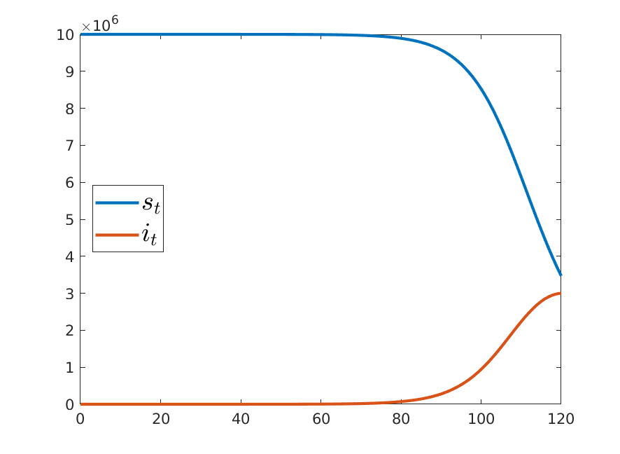
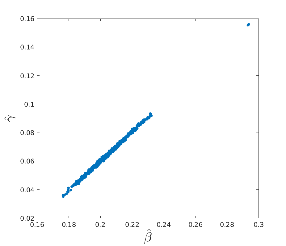
Figure 1: The trajectory of the SIR model used in the simulation (left). Plots of $\hat{\beta}$ vs $\hat{\gamma}$ from 1000 realizations from the sampling distribution of their MLE (right).

The linear shape of the plot in Figure 1 suggests a practical identifiability problem in this model. That is, while the MLE exists and is unique, the curvature of the log-likelihood in the neighborhood of the MLE is very small in the direction where $\hat{\beta},\hat{\gamma}$ lie along a line. We are not the first to notice this phenomenon. Previous works include Chis2011; Hamelin2020; Lee2020; Tuncer2018, which experience qualitatively similar issues despite notable differences in the formulation of the likelihood in those settings.

While various empirical studies exist, our main contribution is a theoretical analysis of this phenomenon and the resulting limitations for solving the inverse problem from noisy observations. We take a two-step approach to the analysis. First, we characterize sensitivity of trajectories $\Delta_{t}$ to perturbations of the parameters $\theta$, and show that perturbations of $\theta$ in the directions $\pi/4$ and $5\pi/4$ (equivalently, along the line of slope $1$ through $\theta$), closely approximate the smallest variation in the trajectory $s_{t}$ among all perturbations for which $\|\theta_{\epsilon}-\theta\|=\epsilon$. We then give a computable approximate lower bound on $\inf_{\theta_{\epsilon}:\|\theta-\theta_{\epsilon}\|=\epsilon}\lvert s_{t}(\theta_{\epsilon})-s_{t}(\theta)\rvert$ for times $t$ prior to the peak infection time. Taken together, these results provide an explanation for the phenomenon in Figure 1.

In the second part of the analysis, we relate the problem of uncertainty quantification to hypothesis tests of the form

$$H_{0}:\theta=\theta_{0}\quad\text{ vs. }\quad H_{1}:\theta=\theta_{\epsilon}$$

for $\|\theta_{\epsilon}-\theta_{0}\|=\epsilon$. We use the result of the first part of our analysis to approximate the type II error of the test, which in turn allows for both theoretical and empirical analysis of the limits of epidemic prediction using SIR models.

3 Results

3.1 Perturbation bound for SIR trajectories

Informally, the phenomenon in Figure 1 is a manifestation of the fact that very different values of $\theta$ can lead to SIR model trajectories that are very close. To formalize this, let $\varphi_{t}(x_{0},\theta)$ be the $(s,i)$-trajectory of the SIR model starting from $x_{0}=(s_{0},i_{0})$ with parameters $\theta=(\beta,\gamma)$. To aid the reader, all relevant notation is summarized in Table 1. We also remark that the analysis in this subsection and its associated appendices, Appendices LABEL:sec:prop1 and LABEL:sec:error, applies directly to the deterministic SIR system (1). In particular, it is independent of our choice of statistical model, which will not become relevant until our discussion of hypothesis testing in Section LABEL:testing.

Notation	Description
$x_{0}=(s_{0},i_{0})$	Shorthand for initial conditions with $s_{0}+i_{0}=1$
$\theta=(\beta,\gamma)$	Shorthand for the parameters of the SIR model
$R_{0}=\beta/\gamma$	The reproductive number
$\delta=\beta-\gamma$	An important combination of the model parameters appearing in later analysis
$\theta_{\epsilon}$	Perturbation of $\theta$ such that $\lVert\theta_{\epsilon}-\theta\rVert=\epsilon$
$\theta_{\epsilon}(\omega)$	Perturbation of $\theta$ in the direction $\omega\in[0,2\pi)$ such that $\lVert\theta_{\epsilon}(\omega)-\theta\rVert=\epsilon$
$\varphi_{t}(x_{0},\theta)=\left(s_{t}(x_{0},\theta),i_{t}(x_{0},\theta)\right)$	Solution of the SIR equation with initial condition $x_{0}$ and parameter $\theta$
$Y_{1:T}$	Observed data on days 1 through $T$
$L(Y_{1:T}|\theta)$	Likelihood of $\theta$ given observed data

Table 1: Summary of notation used throughout this article.

For $\epsilon>0$, let $S_{\epsilon}(\theta)$ denote the circle of radius $\epsilon$ about $\theta$. That is,

$$S_{\epsilon}(\theta)=\{\theta_{\epsilon}(\omega):\omega\in[0,2\pi)\}$$

where $\theta_{\epsilon}(\omega)=\theta+\epsilon(\cos(\omega),\sin(\omega))$. We set $\delta=\beta-\gamma$ and assume throughout that $\delta>0$; if not, then the reproductive number $R_{0}=\beta/\gamma$ is at most 1 and the epidemic does not grow even at time 0. Similarly, we assume $\epsilon<\delta$. This ensures $R_{0}$ values of the perturbed parameters $\theta_{\epsilon}(\omega)=(\beta+\epsilon\cos(\omega),\gamma+\epsilon\sin(\omega))$ are also strictly greater than 1

$$\beta+\epsilon\cos(\omega)-\gamma-\epsilon\sin(\omega)=\delta+\epsilon(\cos(\omega)-\sin(\omega))\geq\delta-\epsilon>0$$

and so $R_{0}(\epsilon,\omega)=(\beta+\epsilon\cos(\omega))/(\gamma+\epsilon\sin(\omega))>1$ for every $\omega$. Finally, for any fixed initial condition $x_{0}$ and parameter $\theta$ we define the peak time, denoted $t_{*}$, to be the deterministic time at which the number of infected individuals $i_{t}(x_{0},\theta)$ is greatest; that is, $t_{*}=\operatorname{argmax}\{i_{t}(x_{0},\theta):t\geq 0\}$. Since $di/dt=0$ if and only if $i=0$ or $s=1/R_{0}$, it is follows that $t_{*}$ exists and is unique whenever $R_{0}>1$. With this notation, the main result of this subsection is the following proposition.

Approximation 1.

Let $\lVert\cdot\rVert$ denote the Euclidean norm on $\mathbb{R}^{2}$ and let $t_{*}$ be the time of peak infection corresponding to $\theta$. Then for all $t\in[0,0.8t_{*})$,

$$\frac{\epsilon}{\delta\sqrt{2}}\big{(}e^{\delta t}-1\big{)}i_{0}\approx\inf_{\omega\in[0,2\pi)}\big{\lVert}\varphi_{t}\big{(}x_{0},\theta_{\epsilon}(\omega)\big{)}-\varphi_{t}(x_{0},\theta)\big{\rVert}.$$ (3)

Furthermore the infimum is approximately achieved when $\omega=\pi/4$ or $5\pi/4$.

The derivation of (3) is in Appendix LABEL:sec:prop1. Approximation 1 says for any perturbation $\theta_{\epsilon}(\omega)$ of $\theta$, the distance between the perturbed trajectory $\varphi_{t}(x_{0},\theta_{\epsilon}(\omega))$ and true trajectory $\varphi_{t}(x_{0},\theta)$ is approximately bounded below by the left side of (3) for all times $t$ up to roughly $80\%$ of $t_{*}$. The “$\approx$” in (3) indicates the bound is subject to error. Specifically, our derivation of Approximation 1 involves two approximations: First, we approximate the SIR model by a differential equation (LABEL:approxODE) whose solution $\widetilde{\varphi}_{t}$ is given by (LABEL:approxsol). Second, we use first-order Taylor expansions to approximate perturbations of $\widetilde{\varphi}_{t}$ resulting from perturbations in parameter space. Despite these approximations, numerical analysis of the error given in Appendix LABEL:sec:error indicates (3) holds for a wide range of parameter values and population sizes; see Figure LABEL:fig2 below and Figure LABEL:fig:logerror in Appendix LABEL:sec:error. This numerical analysis also motivates our choice of $80\%$ of the peak time as a cutoff, though this cutoff can be extended to $85\%$ or even $90\%$ for larger populations and certain parameter values; see Table LABEL:tab:percentpeak. To complement the numerical results of Appendix LABEL:sec:error, we give a theoretical upper bound on the error in Appendix LABEL:sec:theory. The theoretical result is more mathematically rigorous than the numerical one; however, it is significantly less precise than the control on error obtained in Appendix LABEL:sec:error. We therefore use results from the numerical analysis, e.g. the 80% threshold, of Appendix LABEL:sec:error rather than the theoretical analysis of Appendix LABEL:sec:theory for the remainder of this paper.