Hill regions of charged three-body systems

Abstract

For charged three-body systems, we discuss the configurations and orientations that are admissible for given values of the conserved total energy and angular momentum. The admissible configurations and orientations are discussed on a configuration space that is reduced by the translational, rotational and dilation symmetries of charged three-body systems. We consider the examples of the charged three-body systems given by the helium atom (two electrons and a nucleus) and the compound of two electrons and one positron. For comparison, the well known example of the Newtonian gravitational three-body system is discussed for the scheme presented in this paper first.

AMS classification numbers: …

1 Introduction

This is the third in a series of three papers where we study charged three-body systems. Following [1] we define $N$-body systems as so-called natural Hamiltonian systems formed by $N$ point masses with position vectors $\mathbf{x}_{i}\in\mathds{R}^{3}$ and masses $m_{i}>0$, $i=1,\ldots,N$, which interact via a potential $V$ that is invariant under the action of the special Euclidean group $\text{SE}(3)=\text{SO}(3)\rtimes\mathds{R}^{3}$, i.e. $V({\text{R}}\,(\mathbf{x}_{1}+a),\ldots,{\text{R}}\,(\mathbf{x}_{N}+a))=V(\mathbf{x}_{1},\ldots,\mathbf{x}_{N})$ for all ${\text{R}}\in\text{SO}(3)$ and $a\in\mathds{R}^{3}$.

More precisely, we define $N$-body systems and their subclass of charged $N$-body systems as follows.

Definition 1.1.

For $M=T^{*}{\mathcal{X}}$ where ${\mathcal{X}}=\mathds{R}^{3N}-\Delta_{c}$ with $\Delta_{c}$ being a closed, possibly empty subset of $\mathds{R}^{3N}$ (the collision set), we call the Hamiltonian system $(M,\omega,H)$, with $\omega$ denoting the standard symplectic form, an $N$-body system with masses $m_{i}>0$ of the $i$-th body, $i=1,\ldots,N$, if $H$ is of the form kinetic plus potential energy

$$H=T+V,$$

where the kinetic energy is $T(p)=\sum_{i}\frac{1}{2m_{i}}p_{i}^{2}$ and the potential $V$ is $\text{SE}(3)$ invariant. We will refer to the system that has potential

$$V(\mathbf{x})=\sum_{i<j}-\frac{\gamma_{ij}}{r_{ij}(\mathbf{x})}$$ (1)

with $r_{ij}=\lVert\mathbf{x}_{i}-\mathbf{x}_{j}\rVert$ and $\gamma_{ij}\in\mathds{R},\quad 1\leq i<j\leq N,$ as the charged $N$-body system. In this case the collision set is given by

$$\Delta_{c}=\{\mathbf{x}=(\mathbf{x}_{1},\ldots,\mathbf{x}_{N})\in\mathds{R}^{3N}\,:\,\mathbf{x}_{i}=\mathbf{x}_{j}\text{ for some }1\leq i<j\leq N\}\,.$$ (2)

We note that this definition of charged $N$-body systems covers besides Coulomb interactions also gravitational interactions and mixtures of these. Depending on the context we will often say particle instead of body.

In the first paper we studied the map of integrals, i.e. the map from the phase space $M=T^{*}{\mathcal{X}}$ to the conserved quantities resulting from the Euclidian symmetries, and the critical points of this map [1]. We in particular showed that as opposed to the gravitational case, the more general charged $N$-body systems can have relative equilibria that are not related to central configurations. We will see an example of such a relative equilibrium in the present paper. The topology of the integral manifolds can change at critical points [2]. As the integral manifolds can also be non-compact they can also change topology at critical points at infinity [2]. We studied such critical points at infinity for charged three body systems in the second paper [3].

The present paper concerns the Hill regions of charged $N$-body systems systems. The notion Hill region alludes to the work of Hill on the accessible region in configuration space of the circular restricted three-body problem for a given value of the energy (or Jacobi constant). For unrestricted $N$-body systems, one first needs to define what is meant by Hill region. To this end it seems natural to first reduce the Euclidian symmetries of $N$-body systems. We will see that the phase space of the reduced system no longer has the structure of a cotangent bundle over a configuration space, and hence the definition of the Hill region as the projection of an energy surface to configuration space like in the restricted case is at first not possible. Reducing in addition to the symplectic Euclidean symmetries the non-symplectic dilation (scaling) symmetry of charged three-body systems we will define their Hill regions in terms of the admissible shapes and orientations for given values of the integrals. Here shapes will refer to equivalence classes of configurations modulo similarity transformations and orientations will refer to the directions of the conserved angular momentum in a body fixed frame of the three-body system.

This paper is organized as follows. In Sec. 2 we represent the symplectic reduction of the Euclidian symmetries of $N$-body systems following to a large extent [4]. In Sec. 3 we make the reduction concrete for three-body systems. What we mean by shapes and orientations will be defined in Sec. 4. Based on theses notions we will define Hill regions in Sec. 5. In Sec. 6 we discuss the critical points where the Hill regions change. In Sec. 7 we discuss three examples of charged three-body systems which includes the well known Newtonian case. A short discussion and an outlook are given in Sec. 8.

2 Reduction of $N$-body systems

As a first step towards defining what we mean by Hill region we reduce the $\text{SE}(3)$ symmetry of a charged three-body system. This reduction can be accomplished symplectically as we will review for general $N$-body systems in this section. We will follow to a large extent [4].

The special Euclidian group $\text{SE}(3)=\text{SO}(3)\rtimes\mathds{R}^{3}$ defines a symplectic group action on the phase space $M=T^{*}{\mathcal{X}}$ of an $N$-body system as defined in Def. 1.1 according to $(\mathbf{x},\mathbf{p})\mapsto(({\text{R}}\,(\mathbf{x}_{1}+\mathbf{a}),\ldots,{\text{R}}\,(\mathbf{x}_{N})+\mathbf{a}),({\text{R}}\,\mathbf{p}_{1},\ldots,{\text{R}}\,\mathbf{p}_{N}))$ for any ${\text{R}}\in\text{SO}(3)$ and $\mathbf{a}\in\mathds{R}^{3}$ where we think of the R as $3\times 3$ orthogonal matrices with unit determinant. The Hamiltonian function in Def. 1.1 is invariant under this action. The $\text{SE}(3)$ symmetry can be reduced successively by reducing the translational symmetry $\mathds{R}^{3}$ first and the rotational symmetry $\text{SO}(3)$ afterwards. The symmetry of translations is easily reduced by choosing Jacobi vectors $\mathbf{s}_{i}\in\mathds{R}^{3},i=1,...,N-1$ (see, e.g., [5] and Sec. 3 for a concrete definition in the case of $N=3$). Together with the position vector of the center of mass of the $N$-body system the Jacobi vectors uniquely determine the positions of the $N$ bodies in space. Due to the absence of external forces, the center of mass of an $N$-body system is moving with a constant velocity and we can choose an inertial frame of reference which has the center of mass at its origin. We view the $\mathbf{s}_{i},i=1,...,N-1$, to be the coordinate vectors of the Jacobi vectors with respect to this center of mass frame. If we now ignore the trivial position of the center of mass then we can view the space of the Jacobi vectors $\mathcal{J}=\mathds{R}^{3(N-1)}$ as the translation reduced configuration space. Taking out the collision set this space becomes $\mathcal{J}\backslash\Delta_{c}$ where $\Delta_{c}$ now is the collision set in terms of the Jacobi vectors (see Sec. 3 for an example). If we moreover ignore the trivial constant momentum of the center of mass we have reduced the phase space to $T^{*}\mathcal{J}\cong(\mathds{R}^{3(N-1)}\backslash\Delta_{c})\times\mathds{R}^{3(N-1)}$.

The metric associated with expressing the kinetic energy $T$ in terms of the velocities corresponding to the Jacobi vectors is diagonal. We will choose the Jacobi vectors to be mass-weighted so that the metric becomes Euclidean, i.e. the kinetic energy assumes the form

$$T=\frac{1}{2}\sum^{N-1}_{i=1}\mathbf{\dot{s}}^{2}_{i}\,.$$ (3)

To address the rotational symmetry we consider a body fixed coordinate frame which is a frame that is related to the center of mass frame by a rotation. Let us denote the coordinate vectors of the Jacobi vectors in the body fixed frame by $\mathbf{r_{i}},i=1,..,N-1$. We then have $\mathbf{s}_{i}={\text{R}}\,\mathbf{r}_{i}$ for some rotation matrix ${\text{R}}\in\text{SO}(3)$. If we identify all configurations that are related by a rotation about the center of mass we get the so called internal space which we denote by $\mathcal{Q}$ and which is formally given by the quotient $\mathbb{R}^{3(N-1)}/\text{SO}(3)$. As the rotation group $\text{SO}(3)$ has dimension 3 (for example Euler angles or Cayley-Klein parameters are coordinates on $\text{SO}(3)$) the internal space $\mathcal{Q}$ has dimension $3(N-2)$. Collinear configurations of the $N$ particles in $\mathds{R}^{3}$ lead to singularities in the reduction. Away from collinear configurations the internal space has a smooth structure (see Sec. 3 for more details). The coordinates on the internal space are called internal coordinates. We will denote the internal space coordinates vectors by ${q}$ and their components by ${q_{{\mu}}}$ with the convention that Greek indices run from 1 to $3(N-2)$. We note that the internal space and the internal coordinates are sometimes also referred to as shape space and shape space coordinates, respectively. We however reserve the term ‘shape’ for definitions that we make below.

We remark that specifying a body-fixed frame can be phrased in the language of gauge theory [4]. One specific choice gives rise to one specific gauge. The reduced Hamiltonian function on the phase space reduced by translations and rotations is again the sum of the kinetic energy and the potential energy. The reduced potential is then a function of the internal coordinates only. The reduced kinetic energy is a function of the internal space coordinates and their conjugate momenta and the rotational degrees of freedom. The reduction can be phrased in such a way that the dependence on the gauge becomes apparent (see also [6, 7]). To see this we make the following definitions.

Let ${\text{R}}\in\text{SO}(3)$ denote the rotation from the center of mass frame to the body frame and $\mathbf{L}$ denote the angular momentum with respect to the center of mass which in terms of the mass weighted Jacobi vectors is given by

$$\mathbf{L}=\sum^{N-1}_{i=1}\mathbf{s}_{i}\times\mathbf{\dot{s}}_{i}.$$ (4)

Then the body velocities and body angular momentum are defined, respectively, by

$$\mathbf{\dot{r}}_{i}={\text{R}}^{T}\mathbf{\dot{s}}_{i},$$ (5)

and

$$\mathbf{J}={\text{R}}^{T}\mathbf{L}\,.$$ (6)

The moment of inertia tensor $\mathbf{M}(q)$ of the $N$-body system is the tensor with components

$$\mathbf{M}_{ij}(q)=\sum^{N-1}_{k=1}(\mathbf{r}_{k}^{2}\delta_{ij}-r_{ki}r_{kj})\,,$$ (7)

where $\mathbf{r}_{k}=(r_{k1},r_{k2},r_{k3})$ in body coordinates. With the so called gauge potential

$$\mathbf{A}_{\mu}(q)=\mathbf{M}^{-1}(q)\cdot\sum_{i=1}^{N-1}\left(\mathbf{r}_{i}\times\frac{\partial\mathbf{r}_{i}}{\partial q_{\mu}}\right)$$ (8)

and the metric

$$g_{\mu\nu}(q)=\sum_{i=1}^{N-1}\frac{\partial\mathbf{r}_{i}(q)}{\partial q_{\mu}}\cdot\frac{\partial\mathbf{r}_{i}(q)}{\partial q_{\nu}}-\mathbf{A}_{\mu}(q)\cdot\mathbf{M}(q)\cdot\mathbf{A}_{\nu}(q)$$ (9)

the kinetic energy becomes

$$K=\frac{1}{2}({\Omega}+\mathbf{A}_{\mu}\dot{q}_{\mu})\cdot\mathbf{M}\cdot({\Omega}+\mathbf{A}_{\nu}\dot{q}_{\nu})\mathbf{+}\frac{1}{2}g_{\mu\nu}\dot{q}_{\mu}\dot{q}_{\nu}\,,$$

where here and in the following we use the Einstein convention of summation over repeated indices. Here ${\Omega}$ is the angular velocity which is obtained by viewing the rotation $R$ relating the space fixed center of mass frame to the body frame to be time dependent and then using the so$(3)$ Lie algebra isomorphism between the skew-symmetric matrix $R^{T}\dot{R}$ and the three-component vector ${\Omega}$ given by

$$\left(\begin{array}[]{ccc}0&-{\Omega}_{3}&{\Omega}_{2}\\ {\Omega}_{3}&0&-{\Omega}_{1}\\ -{\Omega}_{2}&{\Omega}_{1}&0\end{array}\right)\mapsto\left(\begin{array}[]{ccc}{\Omega}_{1}\\ {\Omega}_{2}\\ {\Omega}_{3}\end{array}\right)\,.$$ (10)

By using the equation

$$\mathbf{J}=\frac{\partial K}{\partial{\Omega}}=\mathbf{M}({\Omega}+\mathbf{A}_{\mu}\dot{q}_{\mu}),$$ (11)

the conjugate momenta of the internal space coordinates are obtained to be

$$p_{\mu}=\frac{\partial K}{\partial\dot{q}_{\mu}}=g_{\mu\nu}\dot{q}_{\nu}+\mathbf{J}\cdot\mathbf{A}_{\mu}\,.$$ (12)

Definition 2.1.

The reduced ro-vibrational Hamiltonian is defined as

$$H(q,p,\mathbf{J})=\frac{1}{2}\mathbf{J}\cdot\mathbf{M}^{-1}\cdot\mathbf{J+}\frac{1}{2}g^{\mu\nu}(p_{\mu}-\mathbf{J}\cdot\mathbf{A}_{\mu})(p_{\nu}-\mathbf{J}\cdot\mathbf{A}_{\nu})+V(q_{1},...,q_{3N-6})\,,$$ (13)

where in order to keep the notation reasonably short we omitted the argument $q$ for $\mathbf{M}$, $\mathbf{A}_{\mu}$ and $g^{\mu\nu}$ even though these are functions of the internal coordinates (see Equations (7) (8) (9)). The first term on the right hand side of (13) is called the rotational or centrifugal kinetic energy and the second term is called the vibrational kinetic energy.

The equations of motion are given by

$$\dot{q}_{\mu}=\partial H/\partial p_{\mu},\ \ \ \dot{p}_{\mu}=-\partial H/\partial q_{\mu},\ \ \ \dot{\mathbf{J}}=\mathbf{J}\times\nabla_{\mathbf{J}}H,$$ (14)

where $\nabla_{\mathbf{J}}H=(\partial_{J_{1}}H,\partial_{J_{2}}H,\partial_{J_{3}}H)$, $\mathbf{J}=(J_{1},J_{2},J_{3})$ and $\mu=1,...,3N-6$ [8]. The equations of motion can be considered to describe a rigid body (the last term) whose time-dependent moment of inertia is determined by the internal ccordinates which together with their conjugate momenta change according to the first two sets of equations. The magnitude $r=\left\|\mathbf{J}\right\|$ of the body angular momentum $\mathbf{J}$ is a constant of motion. Away from collinear configurations, the phase space of the reduced system with a magnitude of the total angular momentum equal to $r$ then has the structure of a product space given by the product of the angular momentum sphere

$$S_{r}^{2}=\{\mathbf{J}\in\mathds{R}^{3}\,|\,J^{2}_{1}+J^{2}_{2}+J^{2}_{3}=r^{2}\}$$ (15)

and the cotangent bundle over the internal space, $T^{*}\mathcal{Q}$, with coordinates $(q_{\mu},p_{\mu})$, $\mu=1,\ldots,3N-6$. As the angular momentum sphere is two-dimensional, the reduced system can be viewed to have $1$ rotational degree of freedom and $3N-6$ vibrational degrees of freedom. The rotational and vibrational degrees of freedom are coupled via the gauge potentials (see Eq. (13)) which give rise to Coriolis terms in the equations of motion.

3 Reduction of three-body systems

In the following we make the reduction described in the previous section more concrete for the case of three-body systems. Consider a system of three bodies with masses $m_{1}$, $m_{2}$ and $m_{3}$ and position vectors $\mathbf{x}_{1},\mathbf{x}_{1},\mathbf{x}_{1}\in\mathbb{R}^{3}$. For the potential (1), we write

$$V(\mathbf{x})=-\frac{\alpha_{3}}{r_{12}(\mathbf{x})}-\frac{\alpha_{2}}{r_{13}(\mathbf{x})}-\frac{\alpha_{1}}{r_{23}(\mathbf{x})}$$ (16)

with $\alpha_{k}\in\mathds{R}$ and $r_{ij}=\lVert\mathbf{x}_{i}-\mathbf{x}_{j}\rVert$, $i,j,k=1,2,3$. We define mass-weighted Jacobi vectors according to

$$\mathbf{s}_{1} = \sqrt{\mu_{1}}(\mathbf{x}_{1}-\mathbf{x}_{3}),$$

$$\mathbf{s}_{2} = \sqrt{\mu_{2}}(\mathbf{x}_{2}-\frac{m_{1}\mathbf{x}_{1}+m_{3}\mathbf{x}_{3}}{m_{1}+m_{3}}),$$

where

$$\mu_{1}=\frac{m_{1}m_{3}}{m_{1}+m_{3}},\ \ \ \mu_{2}=\frac{m_{2}(m_{1}+m_{3})}{m_{1}+m_{2}+m_{3}}$$ (17)

are the reduced masses of the two-body systems with masses $m_{1}$ and $m_{3}$ and $m_{2}$ and $m_{1}+m_{3}$, respectively (see Fig. 1).

As mentioned in Sec. 2 we can view the space $\mathcal{J}=\mathds{R}^{3}\times\mathds{R}^{3}$ of Jacobi vectors $\mathbf{s}_{1}$ and $\mathbf{s}_{2}$ as the translation reduced configuration space. Viewing the Jacobi vectors as column vectors of $3\times 2$ matrices we can identify the configuration space with the space of $3\times 2$ matrices $\mathds{R}^{3\times 2}$. The translation reduced configuration space $\mathcal{J}$ can then be viewed as the disjoint union [9]

$$\mathcal{J}={\mathcal{J}_{{0}}}\cup{\mathcal{J}_{{1}}}\cup{\mathcal{J}_{{2}}}\,,$$ (18)

where for $k=0,1,2$,

$${\mathcal{J}_{{k}}}:=\{A\in\mathds{R}^{3\times 2}\,:\,\text{rank}A=k\}\,.$$ (19)

Here ${\mathcal{J}_{{2}}}$ contains the non-collinear configurations, ${\mathcal{J}_{{1}}}$ contains the collinear configurations, and ${\mathcal{J}_{{0}}}$ the triple collision (which is the centre of mass located at the origin). We note that for systems with more than three particles, $\mathcal{J}$ in (18) also contains the union with ${\mathcal{J}_{{3}}}$ (defined in an analogous way). For three particles, ${\mathcal{J}_{{3}}}$ is empty. Moreover, ${\mathcal{J}_{{2}}}$ is a smooth manifold whose boundary is formed by ${\mathcal{J}_{{0}}}\cup{\mathcal{J}_{{1}}}$, i.e. $\partial{\mathcal{J}_{{2}}}={\mathcal{J}_{{0}}}\cup{\mathcal{J}_{{1}}}$.

The collision set is given by

$$\Delta_{c}=\{(\mathbf{s}_{1},\mathbf{s}_{2})\in\mathds{R}^{3}\times\mathds{R}^{3}\,:\,\mathbf{s}_{1}=0,\,\mathbf{s}_{2}=\frac{\sqrt{\mu_{2}}}{\sqrt{\mu_{1}}}\frac{m_{1}}{m_{1}+m_{3}}\mathbf{s}_{1},\text{ or }\mathbf{s}_{2}=\frac{\sqrt{\mu_{2}}}{\sqrt{\mu_{1}}}\frac{m_{3}}{m_{1}+m_{3}}\mathbf{s}_{1}\},$$ (20)

where the conditions defining the set correspond to collisions of particles 1 and 3, 2 and 3, and 1 and 2, in this order. The collision set is contained in the boundary of ${\mathcal{J}_{{2}}}$, i.e. $\Delta_{c}\subset\partial{\mathcal{J}_{{2}}}$. Let

$$\Delta_{c,k}:=\Delta\cap{\mathcal{J}_{{k}}}$$ (21)

for $k=0,1,2$. Then $\Delta_{c,2}$ is empty, and $\Delta$ equals the disjoint union of $\Delta_{c,1}$ and $\Delta_{c,0}$, where $\Delta_{c,1}$ contains the double collisions which are no triple collisions and $\Delta_{c,0}$ contains the triple collision.

The rotation group $\text{SO}(3)$ acts on $\mathcal{J}$ according to

$$(\mathbf{s}_{1},\mathbf{s}_{2})\mapsto({\text{R}}\,\mathbf{s}_{1},{\text{R}}\,\mathbf{s}_{2}),\quad{\text{R}}\in\text{SO}(3).$$ (22)

The internal space $\mathcal{Q}$ is then the quotient space $\mathcal{J}/\text{SO}(3)$ which consists of the equivalence classes of configurations that can be mapped to one another via a rotation ${\text{R}}\in\text{SO}(3)$. Let $\pi:\mathcal{J}\to\mathcal{J}/\text{SO}(3)$ denote the quotient map. For $(\mathbf{s}_{1},\mathbf{s}_{2})\in\mathcal{J}$, let $\mathcal{O}_{(\mathbf{s}_{1},\mathbf{s}_{2})}:=\{({\text{R}}\,\mathbf{s}_{1},{\text{R}}\mathbf{s}_{2})\,:\,{\text{R}}\in\text{SO}(3)\}$ be the $\text{SO}(3)$ orbit through $(\mathbf{s}_{1},\mathbf{s}_{2})$ and $\mathcal{G}_{(\mathbf{s}_{1},\mathbf{s}_{2})}:=\{{\text{R}}\in\text{SO}(3)\,:\,({\text{R}}\,\mathbf{s}_{1},{\text{R}}\,\mathbf{s}_{2})=(\mathbf{s}_{1},\mathbf{s}_{2})\}$ the isotropy group at $(\mathbf{s}_{1},\mathbf{s}_{2})$. Then

$$\mathcal{G}_{(\mathbf{s}_{1},\mathbf{s}_{2})}=\left\{\begin{array}[]{cl}\{e\}&\text{ for }(\mathbf{s}_{1},\mathbf{s}_{2})\in{\mathcal{J}_{{2}}},\\ \text{SO}(2)&\text{ for }(\mathbf{s}_{1},\mathbf{s}_{2})\in{\mathcal{J}_{{1}}},\\ \text{SO}(3)&\text{ for }(\mathbf{s}_{1},\mathbf{s}_{2})\in{\mathcal{J}_{{0}}},\end{array}\right.$$ (23)

and

$$\mathcal{O}_{(\mathbf{s}_{1},\mathbf{s}_{2})}=\left\{\begin{array}[]{cl}\text{SO}(3)&\text{ for }(\mathbf{s}_{1},\mathbf{s}_{2})\in{\mathcal{J}_{{2}}},\\ S^{2}&\text{ for }(\mathbf{s}_{1},\mathbf{s}_{2})\in{\mathcal{J}_{{1}}},\\ \{0\}&\text{ for }(\mathbf{s}_{1},\mathbf{s}_{2})\in{\mathcal{J}_{{0}}}.\end{array}\right.$$ (24)

The configuration space can hence be viewed to be stratified into three strata defined via the orbit type, i.e. $\mathcal{J}={\mathcal{J}_{{2}}}\cup{\mathcal{J}_{{1}}}\cup{\mathcal{J}_{{0}}}$, and the projection is similarly stratified according to

$${\mathcal{J}_{{2}}}\to{\mathcal{J}_{{2}}}/\text{SO}(3),\quad{\mathcal{J}_{{1}}}\to{\mathcal{J}_{{1}}}/\text{SO}(3),\text{ and }{\mathcal{J}_{{0}}}\to{\mathcal{J}_{{0}}}/\text{SO}(3).$$ (25)

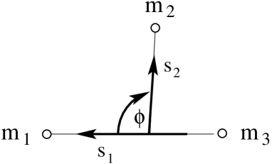
Figure 1: Directions of the mass weighted Jacobi vectors $\mathbf{s}_{1}$ and $\mathbf{s}_{2}$. The vector $\mathbf{s}_{2}$ has its tail at the centre of mass of the particles 1 and 3. The Jacobi coordinates $\rho_{1}$ and $\rho_{2}$ are the lengths of the vectors $\mathbf{s}_{1}$ and $\mathbf{s}_{2}$, respectively, and $\phi$ is the angle between the two vectors.

As coordinates on the internal space we can take the Jacobi coordinates $(\rho_{1},\rho_{2},\phi)$ defined as

$$\rho_{1}=\|\mathbf{s}_{1}\|\,,\quad\rho_{2}=\|\mathbf{s}_{2}\|\,,\quad\mathbf{s}_{1}\cdot\mathbf{s}_{2}=\rho_{1}\,\rho_{2}\,\cos\phi\,,$$

where $0\leq\phi\leq\pi$ (see Fig. 1).

Let $\{\boldsymbol{e}_{1},\boldsymbol{e}_{2},\boldsymbol{e}_{3}\}$ be the standard basis in $\mathds{R}^{3}$. Then we can define a section $\sigma:\mathcal{J}/\text{SO}(3)\to\mathcal{J}$ as

$$\sigma(\rho_{1},\rho_{2},\phi)=(\mathbf{r}_{1},\mathbf{r}_{2}):=(\rho_{1}\boldsymbol{e}_{1},\rho_{2}\cos\phi\,\boldsymbol{e}_{1}+\rho_{2}\sin\phi\,\boldsymbol{e}_{2}).$$ (26)

This section is called the $xxy$-gauge in [4] as it corresponds to the choice of a body frame where two bodies (bodies 1 and 3 in our case) are located on the $x$ axis and the third body (body 2) is contained in the $xy$ plane. The mass weighted Jacobi vectors $(\mathbf{s}_{1},\mathbf{s}_{2})$ of the three-body system are then given by

$$(\mathbf{s}_{1},\mathbf{s}_{2})=({\text{R}}\,\mathbf{r}_{1},{\text{R}}\,\mathbf{r}_{2})=(\rho_{1}{\text{R}}\,\boldsymbol{e}_{1},\rho_{2}\cos\phi\,{\text{R}}\,\boldsymbol{e}_{1}+\rho_{2}\sin\phi\,{\text{R}}\,\boldsymbol{e}_{2})$$ (27)

for some ${\text{R}}\in\text{SO}(3)$.

Collinear configurations are given in terms of the Jacobi coordinates by either of the equalities $\phi=0$, $\phi=\pi$ and $\rho_{2}=0$. For $\rho_{1}=0$ (in which case $\phi$ is not defined), particles 1 and 3 collide. For $\phi=0$ combined with $\rho_{2}=\frac{m_{3}}{m_{1}+m_{3}}\frac{\sqrt{\mu_{2}}}{\sqrt{\mu_{1}}}\rho_{1}$, particles 1 and 2 collide. For $\phi=\pi$ combined with $\rho_{2}=\frac{m_{1}}{m_{1}+m_{3}}\frac{\sqrt{\mu_{2}}}{\sqrt{\mu_{1}}}\rho_{1}$, particles 1 and 3 collide. At the triple collision $\rho_{1}=\rho_{2}=0$.

Besides the Jacobi coordinates another natural choice of coordinates is given by the inter particle distances $r_{12}$, $r_{13}$ and $r_{23}$ which besides being nonnegative need to satisfy the triangle inequality $r_{12}+r_{13}\geq r_{23}$ and its cyclic permutations. Collinearity is given by equality in either of the triangle inequalites. Double collisions between two particles are obviously given by the corresponding distance being zero. At the triple collision all distances are vanishing.

As will become clear below for the discussion of the Hill regions, it is useful to introduce yet another coordinate system. To this end we first define

$$(w_{1},w_{2},w_{3})=(\rho_{1}^{2}-\rho_{2}^{2},2\,\rho_{1}\,\rho_{2}\cos\phi,2\,\rho_{1}\,\rho_{2}\,\sin\phi)\,,$$ (28)

where $w_{1},w_{2}\in\mathds{R}$ and $w_{3}\geq 0$. Equation (28) shows that the Jacobi coordinates are confocal parabolic coordinates in the space of the coordinates $(w_{1},w_{2},w_{3})$. The coordinate $w_{3}$ is twice the area of the parallelogram spanned by the Jacobi vectors $\mathbf{s}_{1}$ and $\mathbf{s}_{2}$. This implies that collinear configurations are contained in the plane $w_{3}=0$. This plane hence also contains the collisions. As double collisions of particles of particles 1 and 3 have $\rho_{1}=0$ we see from (28) that these are located on the negative $w_{1}$ axis. Double collisions of particles 1 and 2 occur on the line in the plane $w_{3}=0$ where

$$\frac{w_{2}}{w_{1}}=2\frac{\sqrt{m_{1}m_{2}m_{3}}\,\sqrt{m_{1}+m_{2}+m_{3}}}{m_{1}(m_{1}+m_{2}+m_{3})-m_{2}m_{3}}.$$ (29)

Similarly collisions of particles 2 and 3 occur in this plane at

$$\frac{w_{2}}{w_{1}}=-2\frac{\sqrt{m_{1}m_{2}m_{3}}\,\sqrt{m_{1}+m_{2}+m_{3}}}{m_{3}(m_{1}+m_{2}+m_{3})-m_{1}m_{2}}.$$ (30)

The triple collision is located at the origin $w_{1}=w_{2}=w_{3}=0$.

The final coordinate system we are considering is then given by spherical coordinates in the $(w_{1},w_{2},w_{3})$ coordinate space which give the Dragt’s coordinates $(\omega,\chi,\psi)$ defined as (see [4] and the references therein)

$$(w_{1},w_{2},w_{3})=(\omega\cos\chi\cos\psi,\omega\cos\chi\sin\psi,\omega\sin\chi)\,,$$ (31)

where $\omega\geq 0$, $0\leq\chi\leq\pi/2$ and $0\leq\psi\leq 2\pi$. Note that $\chi$ is the latitude, not the colatitude, and $\omega=\rho_{1}^{2}+\rho_{2}^{2}$.

For completeness, we also give the expressions for the inter particle distances in terms of Dragt’s coordinates:

$$\begin{split}r_{12}&=\frac{1}{\sqrt{2\mu_{1}}}\sqrt{\omega+\omega\cos\chi\cos\psi}\,,\\ r_{13}&=\sqrt{\frac{\mu_{1}}{2m_{1}^{2}}(\omega+\omega\cos\chi\cos\psi)+\frac{1}{2\mu_{2}}(\omega-\omega\cos\chi\cos\psi)-\frac{\sqrt{\mu_{1}}}{m_{1}\sqrt{\mu_{2}}}\omega\cos\chi\sin\psi}\,,\\ r_{23}&=\sqrt{\frac{\mu_{1}}{2m_{3}^{2}}(\omega+\omega\cos\chi\cos\psi)+\frac{1}{2\mu_{2}}(\omega-\omega\cos\chi\cos\psi)+\frac{\sqrt{\mu_{1}}}{m_{3}\sqrt{\mu_{2}}}\omega\cos\chi\sin\psi}\,.\end{split}$$ (32)

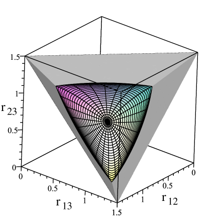
Figure 2: The coordinate surface $\omega=1$ of the Dragt’s coordinates in the space of the inter particle distances $r_{12}$, $r_{13}$ and $r_{23}$. This surface can be viewed as the shape space $\tilde{\mathcal{Q}}$ defined in (49).

By choosing the internal coordinates as the Jacobi coordinates ($\rho_{1},\rho_{2},\phi$) the inertia tensor becomes [4]

$$\mathbf{M}=\left[\begin{array}[]{ccc}\rho_{2}^{2}\sin^{2}\phi&-\rho_{2}^{2}\sin\phi\cos\phi&0\\ -\rho_{2}^{2}\sin\phi\cos\phi&\rho_{1}^{2}+\rho_{2}^{2}\cos^{2}\phi&0\\ 0&0&\rho_{1}^{2}+\rho_{2}^{2}\end{array}\right]\,.$$ (33)

Its eigenvalues give the principal moments of inertia

$$M_{1/2}=\frac{1}{2}\big{(}\rho_{1}^{2}+\rho_{2}^{2}\mp\sqrt{\rho_{1}^{4}+\rho_{2}^{4}+2\cos(2\phi)\rho_{1}^{2}\rho_{2}^{2}}\,\big{)}$$ (34)

and $M_{3}=\rho_{1}^{2}+\rho_{2}^{2}$. The metric and the gauge potential become

$$\left[g_{\mu\nu}\right]=\left[\begin{array}[]{ccc}1&0&0\\ 0&1&0\\ 0&0&\frac{\rho_{1}^{2}\rho_{2}^{2}}{\rho_{1}^{2}+\rho_{2}^{2}}\end{array}\right]$$ (35)

and

$$\mathbf{A}_{\rho_{1}}=\mathbf{A}_{\rho_{2}}=(0,0,0),\ \ \ \mathbf{A}_{\phi}=(0,0,\frac{\rho_{2}^{2}}{\rho_{1}^{2}+\rho_{2}^{2}}).$$ (36)

In Dragt’s coordinates the inertia and metric tensors are diagonal [4]:

$$\mathbf{M}=\left[\begin{array}[]{ccc}\omega\sin^{2}\frac{\chi}{2}&0&0\\ 0&\omega\cos^{2}\frac{\chi}{2}&0\\ 0&0&\omega\end{array}\right]$$ (37)

and

$$\left[g_{\mu\nu}\right]=\frac{1}{4}\,\left[\begin{array}[]{ccc}\frac{1}{\omega}&0&0\\ 0&\omega&0\\ 0&0&\omega\cos^{2}\chi\end{array}\right]\,,$$ (38)

In particular the principal moments of inertia $M_{1}=\omega\sin^{2}\frac{\chi}{2}$, $M_{2}=\omega\cos^{2}\frac{\chi}{2}$ and $M_{3}=\omega$ are ordered by magnitude on the diagonal of $\mathbf{M}$ (note that $0\leq\chi\leq\pi/2$).

The gauge potential becomes in this case

$$\mathbf{A}_{\omega}=\mathbf{A}_{\chi}=(0,0,0),\ \ \ \mathbf{A}_{\psi}=(0,0,-\frac{1}{2}\sin\chi).$$ (39)

Remark 3.1.

The first and second principal moments of inertia add up to the third (see, e.g., (37)):

$$M_{1}+M_{2}=M_{3}\,.$$ (40)

It follows from our choice of the $xxy$-gauge that the principal moment of inertia $M_{3}$ corresponds to the axis of rotation that contains the centre of mass and is perpendicular to the plane in which the three bodies are lying. In the celestial mechanics literature $M_{3}$ is simply referred to as moment of inertia (see, e.g., [10]), and it is common to use the symbol $I$ for it. In Jacobi and Dragt’s coordinates, respectively, it is then given by

$$I:=M_{3}=\frac{1}{2}\text{tr}\,M=\rho_{1}^{2}+\rho_{2}^{2}=\omega.$$ (41)

This will play an important role in Sec. 4.

Remark 3.2.

The moment of inertia tensor is a smooth function on the internal space $\mathcal{Q}$. However, whereas the third principal moment of inertia $M_{3}$ is a smooth function on the internal space $\mathcal{Q}$, the first and the second principal moments of inertia $M_{1}$ and $M_{2}$ are continuous on $\mathcal{Q}$ and smooth only at points $q\in\mathcal{Q}$ where $M_{1}(q)\neq M_{2}(q)$. This can be seen from using Jacobi coordinates $\rho_{1}$, $\rho_{2}$ and $\phi$ which as opposed to Dragt’s coordinates are smooth coordinates on the interior of the internal space (i.e. away from collinear configurations). The principal moments of inertia $M_{1}$ and $M_{2}$ are not differentiable when the square root in (34) vanishes which happens only for $\rho_{1}=\rho_{2}$ together with $\phi=\pi/2$, i.e. when $M_{1}=M_{2}$. In quantum physics such singular points of parameter families of Hermitian operators are referred to as diabolic points and we follow this terminology. The diabolic points of the moment of inertia tensor have $(w_{1},w_{2},w_{3})=(0,0,w)$ and the angle $\chi$ of Dragt’s coordinates is not defined. In fact it is not possible to have smooth coordinates on the internal space in terms of which the moment of inertial tensor is diagonal.

Remark 3.3.

Collinear configurations (which include double collisions) are given in Jacobi coordinates by $\phi=0$, $\phi=\pi$, $\rho_{2}=0$ or $\rho_{1}=0$ where the latter always corresponds to a double collision, and in Dragt’s coordinates by $\chi=0$, i.e. $w_{3}=0$, and hence $w_{1}^{2}+w_{2}^{2}=\omega^{2}$. Here $M_{1}=0$ and $M_{2}=M_{3}=\rho_{2}^{2}=\omega$.

4 Dilation symmetry and the shape-orientation space

As the next step towards our definition of a Hill region we reduce the non-symplectic scaling symmetry of charged three-body systems. After having reduced the translational and rotational symmetries in Secs. 2 and 3 the reduction of this scaling will lead to our notion of the shape and orientation of a charged three-body system which will then enter our definition of a Hill region in Sec. 5.

The potential $V$ in (16) and the inertia tensor $\mathbf{M}$ with the components given in (7) are homogenous functions of the distances between the particles of degree $-1$ and $2$, respectively. We make this more formal by defining an $\mathds{R}$ action as follows.

Definition 4.1.

The dilation transformation is the $\mathds{R}$ action on the translation-reduced configuration space $\mathcal{J}$ defined as

$$d:\mathds{R}\times\mathcal{J}\to\mathcal{J},\quad(l,(\mathbf{s}_{1},\mathbf{s}_{2}))\mapsto(\mathrm{e}^{l}\mathbf{s}_{1},\mathrm{e}^{l}\mathbf{s}_{2}).$$ (42)

We write

$$d_{\lambda}(\mathbf{s}_{1},\mathbf{s}_{2})=(\lambda\mathbf{s}_{1},\lambda\mathbf{s}_{2})\,,$$ (43)

where $\lambda=\mathrm{e}^{l}>0$.

The dilation transformation defines a singular line bundle $\mathcal{J}\to\mathcal{J}/\mathds{R}$. The only point with nontrivial isotropy is the triple collision point. The bundle $({\mathcal{J}_{{2}}}\cup{\mathcal{J}_{{1}}})\to({\mathcal{J}_{{2}}}\cup{\mathcal{J}_{{1}}})/\mathds{R}$ is smooth. The dilation $\mathds{R}$ action commutes with the $\text{SO}(3)$ action in (22), i.e. $d_{\lambda}({\text{R}}\,\mathbf{s}_{1},{\text{R}}\,\mathbf{s}_{2})=(\lambda{\text{R}}\,\mathbf{s}_{1},\lambda{\text{R}}\,\mathbf{s}_{2})=({\text{R}}\lambda\mathbf{s}_{1},{\text{R}}\lambda\mathbf{s}_{2})$ for all $\lambda>0$ and ${\text{R}}\in\text{SO}(3)$. As we can identify the internal space $\mathcal{Q}=\mathcal{J}/\text{SO}(3)$ with the (image of the) section given by the $xxy$-gauge the dilation transformation also ‘induces’ a map on the internal space $\mathcal{Q}$. From (26) we get

$$d_{\lambda}(\mathbf{r}_{1},\mathbf{r}_{2})=(\lambda\rho_{1}\boldsymbol{e}_{1},\lambda\rho_{2}\cos\phi\,\boldsymbol{e}_{1}+\lambda\rho_{2}\sin\phi\,\boldsymbol{e}_{2}),$$ (44)

i.e. in Jacobi the induced dilation map $\mathcal{Q}\to\mathcal{Q}$, $q\mapsto d_{\lambda}(q)$ reads

$$d_{\lambda}(\rho_{1},\rho_{2},\phi)=(\lambda\rho_{1},\lambda\rho_{2},\phi).$$ (45)

In terms of Dragt’s coordinates the map becomes

$$d_{\lambda}(\omega,\chi,\psi)=(\lambda^{2}\omega,\chi,\psi).$$ (46)

In order to avoid a cumbersome notation we here use the same symbol for the induced map as in (43).

Homogeneity of $V$ and $\mathbf{M}$ now means that

$$V(d_{\lambda}(q))=\lambda^{-1}V(q)\quad\text{ and }\quad\mathbf{M}(d_{\lambda}(q))=\lambda^{2}\mathbf{M}(q)\,.$$ (47)

For the moment of inertia $I$ defined in (41), we similarly have

$$I(d_{\lambda}(q))=\lambda^{2}I(q).$$ (48)

In fact the (induced) dilation map also defines a line bundle $\mathcal{Q}\to\mathcal{Q}/\mathds{R}$. For this bundle, we can construct a section by noting that except for the triple collision point we can find for each point $q\in\mathcal{Q}$ a $\lambda>0$ such that for the moment of inertia defined in (41) we have $I(d_{\lambda}(q))=1$. We can then identify the quotient space $\mathcal{Q}/\mathds{R}$ with this section.

Definition 4.2.

The shape space is the dilation reduced interior of the internal space given by

$$\tilde{\mathcal{Q}}:=\{q\in\mathcal{Q}^{\mathrm{o}}\,:\,I(q)=1\}.$$ (49)

The points in the shape space are referred to as shapes and denoted by $\tilde{q}$.

The boundary of the shape space (which is not part of the shape space) consists of collinear configurations. We excluded collinear configurations in the definition of the shape space to avoid difficulties resulting from singularities in the reduction of the rotational symmetry.

We can identify the shape space $\tilde{\mathcal{Q}}$ with the upper hemisphere of the unit sphere in the coordinate space $(w_{1},w_{2},w_{3})$ on which we can use $(w_{1},w_{2})$ or Dragt’s coordinates $(\chi,\psi)$ as coordinates. Note however that the latter are singular at the pole $(w_{1},w_{2},w_{3})=(0,0,1)$. For comparison, $\tilde{\mathcal{Q}}$ is shown in the space of inter particle distances in Fig. 2. The orbits of the dilation $\mathds{R}$ action in the internal spaces with coordinates $(w_{1},w_{2},w_{3})$ and $(d_{12},d_{13},d_{23})$ are straight line rays emanating from (but not including) the origin which corresponds to the triple collision point. In view of the definition of the shape space according to (49) we can view the shape space to form a submanifold of the internal space and this way also can define the action of the dilation transformation $d_{\lambda}$ on points $\tilde{q}\in\tilde{\mathcal{Q}}$. For $q=\tilde{q}$ with $q\in\mathcal{Q}$, we set $d_{\lambda}(\tilde{q}):=d_{\lambda}(q)$. Let

$$\tilde{V}:=\left.V\right|_{\tilde{Q}}\quad\text{ and }\quad\mathbf{\tilde{M}}:=\left.\mathbf{M}\right|_{\tilde{Q}}.$$ (50)

Then for $\tilde{q}\in\tilde{Q}$,

$$V(d_{\lambda}(\tilde{q}))=\lambda^{-1}\tilde{V}(\tilde{q})\quad\text{ and }\quad\mathbf{M}(d_{\lambda}(\tilde{q}))=\lambda^{2}\mathbf{\tilde{M}}(\tilde{q}).$$ (51)

Let $\tilde{M}_{k}$, $k=1,2,3$, be the dilation reduced principal moments of inertia, i.e. the eigenvalues of $\mathbf{\tilde{M}}$. Then by construction $\tilde{M}_{3}$ is constant 1 on the the shape space $\tilde{Q}$. The graphs of $\tilde{M}_{1}$ and $\tilde{M}_{2}$ over the shape space considered as the unit disk in the $(w_{1},w_{2})$-plane are shown in Fig. 3. Inline with Remark 3.2, we see that the graphs are not smooth at the diabolic point $w_{1}=w_{2}=0$ where $\tilde{M}_{1}=\tilde{M}_{2}$. Note the rotational symmetry in Fig. 3 resulting from the independence of the principal moments of inertia in (37) from the angle $\psi$. This means that there are loops in the internal space and shape space along which the principal moments are constant.

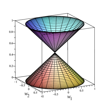
Figure 3: Graphs of the principal moments of inertia $\tilde{M}_{1}$ (lower cone) and $\tilde{M}_{2}$ (upper cone) over the shape space given by the unit disk in the $(w_{1},w_{2})$-plane showing the diabolic point in Remark 3.2.

In addition to the shape space we define the normalised body angular momenta

$$\mathbf{\tilde{J}}=\frac{1}{\|\mathbf{J}\|}\mathbf{J}$$ (52)

and the normalised angular momentum sphere

$$S^{2}_{1} = \{\mathbf{\tilde{J}}\in\mathds{R}^{3}\,:\,\tilde{J}_{1}^{2}+\tilde{J}_{2}^{2}+\tilde{J}_{3}^{2}=1\}.$$ (53)

Whereas the shape space determines the shape formed by the $3$ bodies the normalised angular momentum sphere $S^{2}_{1}$ contains information about the orientation of the $3$-body system in space. In fact, a point on $S^{2}_{1}$ specifies the direction of the conserved space fixed angular momentum $\mathbf{L}$ in the body frame. This fixes the orientation of the three-body system in space up to the angle of rotation of the three-body system about the axis through the center of mass with the direction of the angular momentum $\mathbf{L}$.

We make the following definition.

Definition 4.3.

The shape-orientation space is the product

$$\tilde{Q}\times S_{1}^{2}.$$ (54)

Points in this product are referred to as shape-orientation points and denoted as $(\tilde{q},\mathbf{\tilde{J}})$.

5 Hill regions

For a given energy $E$, the Hill region of a Hamiltonian system whose phase space is a cotangent bundle over configuration space is in general defined as the projection of the energy surface to configuration space. As the angular momentum is conserved for $N$-body systems it is useful to not only consider the projection of the energy surface but the projection of the integral manifold where both the energy and the angular momentum are fixed. Furthermore it is useful to consider the projection of the integral manifold to a space reduced by the symmetries of translations and rotations and, for charged $N$-body systems, also by dilations. The reduced phase space is then however no longer a cotangent bundle (see Sec. 2) and it needs to be defined what a Hill region should be in this case. We do this as follows.

Definition 5.1.

For given value $E$ of the energy and magnitude $r>0$ of the angular momentum (i.e. $r=\|\mathbf{L}\|>0$), we say that a shape-orientation point $(\tilde{q},\mathbf{\tilde{J}})$ is in the Hill region if for the Hamiltonian function $H(q,p,\mathbf{J})$ in (13), there exists a $\lambda>0$ and $p$ such that

$$H(d_{\lambda}(\tilde{q}),p,r\mathbf{\tilde{J}})=E.$$ (55)

For computations, it is useful to have the following characterisation.

Lemma 5.1.

For given values of the energy $E=H$ and magnitude of the angular momentum $r=\|\mathbf{L}\|>0$, a shape-orientation point $(\tilde{q},\mathbf{\tilde{J}})$ is in the Hill region if and only if there exists a $\lambda>0$ such that

$$F(\lambda):=\lambda^{2}\,E-r^{2}\frac{1}{2}\mathbf{\tilde{J}}\cdot[\mathbf{\tilde{M}}(\tilde{q})]^{-1}\cdot\mathbf{\tilde{J}}-\lambda\,\tilde{V}(\tilde{q})\geq 0,$$ (56)

where $\tilde{V}$ and $\mathbf{\tilde{M}}$ are the restrictions of $V$ and $\mathbf{M}$ to the shape space (see (50)).

Proof.

As the metric $g^{\mu\nu}$ is positive definite the vibrational kinetic energy (the second term in the Hamiltonian in (13)) is nonnegative, we can satisfy the energy equation (55) for some $\lambda>0$ and $p$ if and only if

$$r^{2}\frac{1}{2}\mathbf{\tilde{J}}\cdot[\mathbf{M}(d_{\lambda}(\tilde{q}))]^{-1}\cdot\mathbf{\tilde{J}}+V(d_{\lambda}(\tilde{q}))\leq E.$$ (57)

By (51) this is equivalent to

$$r^{2}\lambda^{-2}\frac{1}{2}\mathbf{\tilde{J}}\cdot[\mathbf{\tilde{M}}(\tilde{q})]^{-1}\cdot\mathbf{\tilde{J}}+\lambda^{-1}\tilde{V}(\tilde{q})\leq E.$$ (58)

Now the inequality $F(\lambda)\geq 0$ in (56) is obtained from multiplying (58) by $\lambda^{2}$ and reordering terms. ∎

From Lemma 5.1 we see that in order to decide whether a shape orientation point $(\tilde{q},\mathbf{J})$ is in the Hill region we need to study the polynomial $F(\lambda)$ with its coefficients being fixed by the given $(\tilde{q},\mathbf{J})$. Let

$$E_{R}=r^{2}\frac{1}{2}\mathbf{\tilde{J}}\cdot\mathbf{\tilde{M}}^{-1}\cdot\mathbf{\tilde{J}}$$ (59)

denote the rotational kinetic energy. For $r>0$, $E_{R}$ is strictly positive. The discriminant of $F(\lambda)$ is then

$$\Delta=4EE_{R}+\tilde{V}^{2}.$$ (60)

The equation of vanishing discriminant, $\Delta=0$, defines a double cone in the space $(E,\tilde{V},E_{R})$, see Fig. 4a, of which only the cone which has $E_{R}\geq 0$ is relevant. For a fixed value of $E_{R}$, the zero discriminant defines a parabola in the $(E,\tilde{V})$ plane (see Fig. 4b). For $E_{R}\to 0$, the parabolas collapse to the negative $E_{R}$-axis. For $E_{R}\to\infty$, the parabolas approach the $\tilde{V}$-axis. For fixed $E_{R}>0$, the parabola together with the coordinate axes divides the $(E,\tilde{V})$-plane into the six regions I, IIa, IIb, IIIa, IIIb and IV marked in Fig. 4b. In the first quadrant of the $(E,\tilde{V})$-plane (region I), $F$ has real roots of which one is positive and the other is negative and $F$ has a minimum that is attained at a positive value of $\lambda$. The second quadrant consists of regions IIa and IIb. In region IIa, $F$ has two negative real roots and a maximum attained at a negative value. In region IIb the roots are complex but $F$ still has a maximum attained at a negative value. The third quadrant consists of regions IIIa and IIIb where in region IIIb the roots are again complex and $F$ still has a maximum which is however now attained at a positive $\lambda$. In region IIIa there are two positive real roots and $F$ has a maximum that is attained for a positive $\lambda$. In region IV in the fourth quadrant $F$ has two real roots of which one is negative and one is positive and $F$ has a minimum that is attained at a negative value of $\lambda$.

We deduce

Theorem 5.1.

Let

$$\lambda_{\pm}:=\frac{\tilde{V}}{2E}\pm\sqrt{\frac{\Delta}{4E^{2}}}$$ (61)

be the roots of $F(\lambda)$ defined in (56) and $r>0$. Then we have:

1. For energies $E>0$, every shape-orientation point belongs to the Hill region.

2. For energies $E<0$, a shape-orientation point with $\tilde{V}>0$ is for no orientation in the Hill region.

3. For energies $E<0$, a shape-orientation point with $\tilde{V}<0$ is in the Hill region if and only if the roots $\lambda_{\pm}$ are real.

It follows from Theorem 5.1 that case 3 where $E,\tilde{V}<0$ requires more attention. For $E,\tilde{V}<0$, the condition to have real roots, $\Delta\geq 0$, is equivalent to

$$\frac{\tilde{V}}{2\sqrt{\frac{1}{2}\mathbf{\tilde{J}}\cdot\mathbf{\tilde{M}}^{-1}\cdot\mathbf{\tilde{J}}}}\leq-\sqrt{-Er^{2}}.$$ (62)

a) b)

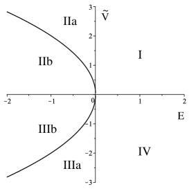
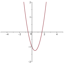
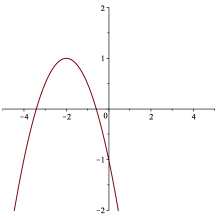
I IIa IIb

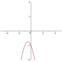
IIIb IIIa IV

Figure 4: Surface of vanishing discriminant of $F(\lambda)$ defined in (56) in the space $(E,\tilde{V},E_{R})$ where $E_{R}=r^{2}\frac{1}{2}\mathbf{\tilde{J}}\cdot\mathbf{\tilde{M}}^{-1}\cdot\mathbf{\tilde{J}}$ is the rotational energy (a). In panel (b) a cut for fixed $E_{R}=1$ in (a) is shown. Together with the coordinate axes it divides the $(E,\tilde{V})$ plane into six regions I, IIa, IIb, IIIa, IIIb and IV. The remaining panels show the graphs of $F:\lambda\mapsto F(\lambda)$ for values of $(E,\tilde{V})$ in these different regions.

With the left hand side of (62) we can define the function

$$\tilde{\mathcal{Q}}\times S_{1}^{2}\to\mathds{R},\quad(\tilde{q},\mathbf{\tilde{J}})\mapsto\frac{\tilde{V}(\tilde{q})}{2\sqrt{\frac{1}{2}\mathbf{\tilde{J}}\cdot(\mathbf{\tilde{M}}(\tilde{q}))^{-1}\cdot\mathbf{\tilde{J}}}}.$$ (63)

The Hill region for given $E<0$ and $r>0$ is then then the sublevel set of this function in $\tilde{Q}\times S_{1}^{2}$ for the value $-\sqrt{-Er^{2}}$. To study the bifurcations of the Hill region we need to study the critical points of the function (63). The critical values can be expressed in terms of

$$\nu:=-Er^{2}$$ (64)

which we can hence view as the bifurcation parameter.

Finding the critical points of the function defined in (63) simplifies to some extent. As $\tilde{V}$ does not depend on $\mathbf{\tilde{J}}$ the $\mathbf{\tilde{J}}$ components of the critical points of the function in (63) are given by the critical points of the function

$$S_{1}^{2}\to\mathds{R},\quad\mathbf{\tilde{J}}\mapsto\frac{1}{2}\mathbf{\tilde{J}}\cdot[\mathbf{\tilde{M}}(\tilde{q})]^{-1}\cdot\mathbf{\tilde{J}}$$ (65)

for fixed shape $\tilde{q}\in\tilde{\mathcal{Q}}$. The critical points of (65) on $S_{1}^{2}$ are $\mathbf{\tilde{J}}$ where the gradients of $\frac{1}{2}\mathbf{\tilde{J}}\cdot[\mathbf{\tilde{M}}(\tilde{q})]^{-1}\cdot\mathbf{\tilde{J}}$ and the function defining the constraint $\mathbf{\tilde{J}}\cdot\mathbf{\tilde{J}}=1$ with respect to $\mathbf{\tilde{J}}$ are parallel. This means that $\mathbf{\tilde{J}}$ is an eigenvector of $\mathbf{\tilde{M}}(\tilde{q})$.

A given shape $\tilde{q}$ can be considered to define a rigid body with moment of inertia tensor $\mathbf{\tilde{M}}$ (where the trace of $\mathbf{\tilde{M}}$ is equal to $1/2$). Apart from the shape corresponding to the diabolic point the shapes $\tilde{q}$ give mutually different principal moments and the corresponding rigid body is asymmetric. Let us at first focus on this case. We will come back to the diabolic point below. For shape coordinates for which the moment of inertia tensor is diagonal like Dragt’s coordinates, the critical values of $\mathbf{\tilde{J}}$ on the normalised angular momentum sphere $S^{2}_{1}$ are then given by $\mathbf{\tilde{J}}$ equal to $(\pm 1,0,0)$, $(0,\pm 1,0)$ or $(0,0,\pm 1)$. The critical (non-diabolic) shapes $\tilde{q}$ are then critical points of the functions

$$\tilde{q}\mapsto\sqrt{\tilde{M}_{k}(\tilde{q})}\,\tilde{V}(\tilde{q}),\quad k=1,2,3,$$ (66)

where the $\tilde{M}_{k}(\tilde{q})$ are the dilation reduced principal moments of inertia. If we use Dragt’s coordinates $(\chi,\psi)$ as shape coordinates then the critical shape-orientations points $(\tilde{q},\mathbf{\tilde{J}})$ are given by the critical points of the functions

$$(\chi,\psi)\mapsto\left\{\begin{array}[]{ccc}\tilde{V}\sin\frac{\chi}{2}&\text{for}&\mathbf{\tilde{J}}=(\pm 1,0,0)\\ \tilde{V}\cos\frac{\chi}{2}&\text{for}&\mathbf{\tilde{J}}=(0,\pm 1,0)\\ \tilde{V}&\text{for}&\mathbf{\tilde{J}}=(0,0,\pm 1)\\ \end{array}\right.$$ (67)

(see (37)).

In the examples in Sec. 7 we will visualise the Hill regions defined according to Definition 5.1 in terms of their projection to the shape space $\tilde{\mathcal{Q}}$. These projections can be understood in terms of the contours of the functions (66) (or (67) when we use Dragt’s coordinates) on $\tilde{\mathcal{Q}}$ as follows. Consider a fixed negative value of the energy $E<0$, a fixed value of the magnitude of the angular momentum $r>0$ and a given shape $\tilde{q}\in\tilde{\mathcal{Q}}$. Let us rewrite the condition for a shape-orientation $(\tilde{q},\mathbf{\tilde{J}})$ to be in the Hill region given by the inequality (62) as

$$-\frac{\tilde{V}(\tilde{q})}{2\sqrt{-Er^{2}}}\geq\tilde{E}_{R}(\mathbf{\tilde{J}}),$$ (68)

where

$$\tilde{E}_{R}(\mathbf{\tilde{J}}):=\frac{1}{2}\mathbf{\tilde{J}}\cdot[\mathbf{\tilde{M}}(\tilde{q})]^{-1}\cdot\mathbf{\tilde{J}}$$ (69)

is the ‘normalised’ rotational energy which gives the rotational energy of a rigid body with moment of inertia tensor $\mathbf{\tilde{M}}(\tilde{q})$ rotating with a total angular momentum of unit magnitude. In Fig. 5 we show the level sets of $\tilde{E}_{R}$ of this rigid body on the unit angular momentum sphere $S_{1}^{2}$ for the case of distinct principal moments of inertia. On $S_{1}^{2}$ the function $\tilde{E}_{R}$ has the three critical values

$$\tilde{E}_{R\,3}:=\frac{1}{2\tilde{M}_{3}(\tilde{q})}<\tilde{E}_{R\,2}:=\frac{1}{2\tilde{M}_{2}(\tilde{q})}<\tilde{E}_{R\,1}:=\frac{1}{2\tilde{M}_{1}(\tilde{q})}$$ (70)

corresponding to a minimum, a saddle and a maximum, respectively. If $-\tilde{V}(\tilde{q})/(2\sqrt{-Er^{2}})<\tilde{E}_{R\,3}$ then the inequality (68) is not satisfied for any point $\mathbf{\tilde{J}}\in S_{1}^{2}$. If $\tilde{E}_{R\,3}<-\tilde{V}(\tilde{q})/(2\sqrt{-Er^{2}})<\tilde{E}_{R\,2}$ then the inequality (68) is satisfied for points $\mathbf{\tilde{J}}\in S_{1}^{2}$ in the ‘caps’ that are given by (closed) disk neighbourhoods of the points $\mathbf{\tilde{J}}=(0,0,\pm 1)$ (see Fig. 5). If $\tilde{E}_{R\,2}<-\tilde{V}(\tilde{q})/(2\sqrt{-Er^{2}})<\tilde{E}_{R\,1}$ then the inequality (68) is satisfied for orientations $\mathbf{\tilde{J}}\in S_{1}^{2}$ in the ‘ring’ that is obtained from excluding two (open) disk neighbourhoods near the poles $\mathbf{\tilde{J}}=(\pm 1,0,0)$ on the unit sphere $\mathbf{\tilde{J}}\in S_{1}^{2}$ . If $\tilde{E}_{R\,1}<-\tilde{V}(\tilde{q})/(2\sqrt{-Er^{2}})$ then the inequality (68) is satisfied for any orientation $\mathbf{\tilde{J}}\in S_{1}^{2}$. The latter two cases are also illustrated in Fig. 5. To illustrate the projection of the Hill region for energy $E$ and magnitude $r$ of the angular momentum to the shape space we will colour each shape $\tilde{q}\in\tilde{\mathcal{Q}}$ if the sublevel set of $\tilde{E}_{R}(\mathbf{\tilde{J}})$ on $S_{1}^{2}$ for the value $-\frac{\tilde{V}(\tilde{q})}{2\sqrt{-Er^{2}}}$ is empty in dark grey, two caps in blue, a ring in red and the full sphere in green.

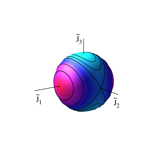
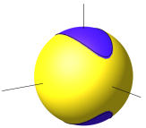
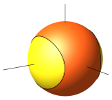
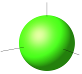
Figure 5: Top panel: level sets of the function defined in (65) on the normalised angular momentum sphere $S_{1}^{2}$ for a fixed shape corresponding to an asymmetric Euler top (with principal moments of inertia $1/3$, $2/3$ and $1$). The function value increases as the colour goes from light blue to red. Lower panel: dependence of the accessible region on the normalised angular momentum sphere on the value of $-\tilde{V}/(2\sqrt{-Er^{2}})$ (see the discussion at the end of Sec. 5).

Let us now come back to the diabolic point, and let us reconsider our approach to compute the critical points of (63) outlined above. The critical points are elements of $\tilde{\mathcal{Q}}\times S_{1}^{2}$. We first determined the components $\mathbf{\tilde{J}}\in S_{1}^{2}$ of the critical points and plugged these in (63) to define the functions (66) whose critical points gave us the components $\tilde{q}\in\tilde{\mathcal{Q}}$ of (63). Here we made use of the fact that we can write the critical $\mathbf{\tilde{J}}\in S_{1}^{2}$ as functions of $\tilde{q}\in\tilde{\mathcal{Q}}$. This tacit use of the Implicit Function Theorem breaks down at the diabolic point where the moments of inertia tensor is degenerate. This is also reflected by the functions (66) not being differentiable at the diabolic point for $k=1,2$. We expect to see signatures of this singularity also in the visualization of the Hill regions in terms of their projection to the shape space when the contours of the function (63) reach $(\tilde{q},\mathbf{\tilde{J}})\in\tilde{\mathcal{Q}}\times S_{1}^{2}$ where $(\tilde{q}$ is the diabolic point and $\mathbf{\tilde{J}}\in S_{1}^{2}$ is an eigenvector of $\mathbf{\tilde{M}}(\tilde{q})$ in the two-dimensional eigenspace for the eigenvalue $\tilde{M}_{1}=\tilde{M}_{2}$. As this point is not a proper critical point of (63) we will refer to it as pseudo critical point.

6 Critical points and bifurcations of the Hill region

In the two preceding papers [1] and [3] we have studied critical points of the map of integrals for charged three-body systems. The integral manifolds, i.e. the joint level sets of the integrals, are expected to change their topology at the corresponding critical values. Due to the non-compact nature of the integral manifolds we had to distinguish between (finite) critical points given by relative equilibria and critical points at infinity. A natural question that arises is how the critical points of the map of integrals are related to the critical points discussed in the previous section. It is to be expected that bifurcations of the integral manifolds also manifest themselves in bifurcations of the Hill regions. Special attention require however critical points of the map of integrals that correspond to points on the boundary of the shape space as we explicitly excluded the boundary from the definition of the shape space and hence of the definition from the Hill regions (see Definitions 4.2 and 5.1, respectively).

In particular the projections of relative equilibria to configuration space can be collinear or non-collinear. The reduction of the $\text{SO}(3)$ symmetry underlying the definition of the Hill region in this paper is singular at collinear configurations even though the corresponding relative equilibria do not have isotropy. The reason for the latter is that at these relative equilibria the momenta are not collinear with the position vectors of the bodies. The singularity of the reduction is due to the fact that the reduction is built on a cotangental lift of the reduction of the configuration space $\text{SO}(3)$ symmetry. There should be a reduction not making use of the cotangent bundle property of the unreduced problem that does not have this problem. Whereas the reduction used in this paper leads a splitting of the rotational and internal degrees of freedom (which however inevitably remain coupled [11]) and preserves the cotangent bundle structure of the phase space for the internal degrees of freedom this is probably no longer the case for a reduction for which the collinear relative equilibria are not singular. These properties of the reduction used in this paper are however in our opinion crucial for a meaningful definition of the Hill region.

So we cannot expect that relative equilibria that project to collinear configurations in configuration space are related to critical points discussed in the previous section. The same however holds for critical points at infinity. For three bodies, a critical point at infinity involves one co-rotating pair of two bodies with the third body at rest at infinity (see Sec. 6.4 below). After scaling such a configuration by the dilation transformation such that the polar moment of inertia $I$ becomes $1$ the co-rotating pair appears to collide. The corresponding shapes are hence also contained in the boundary of the shape space.

The only question that remains is then how the critical points in Sec. 5 are related to non-collinear relative equilibria. The latter are the stationary solutions of the reduced equations of motion (14). They satisfy the equations [8]

$$\mathbf{J}\times\left(\mathbf{M}^{-1}\cdot\mathbf{J}\right) = 0,$$ (71)

$$p_{\mu} = \mathbf{J}\cdot\mathbf{A}_{\mu},$$ (72)

$$\frac{\partial}{\partial q_{\mu}}(\frac{1}{2}\mathbf{J}\cdot\mathbf{M}^{-1}\cdot\mathbf{J}+V(q)) = 0.$$ (73)

Equation (71) implies that at relative equilibria the body angular momentum $\mathbf{J}$ is an eigenvector of the moment of inertia tensor, i.e. $\mathbf{J}$ is parallel to a principal axis. This means that the three-body system is rotating about one of its principal axes. Using this fact the internal coordinates of relative equilibria can be found from the critical points of the effective potential

$$V_{\text{eff}}(q):=\frac{1}{2}\mathbf{J}\cdot[\mathbf{M}(q)]^{-1}\cdot\mathbf{J}+V(q)\,,$$ (74)

where $\mathbf{J}$ is a fixed vector of a given modulus $r$ parallel to a chosen principal axis.

For rotations about the first, second or third principal axis where $\mathbf{J}=(\pm r,0,0)$, $\mathbf{J}=(0,\pm r,0)$ or $\mathbf{J}=(0,0,\pm r)$, respectively, the effective potential becomes

$$V_{\text{eff}}(q)=\frac{1}{2}\frac{r^{2}}{M_{k}(q)}+V(q)\,,\quad k=1,2,3.$$ (75)

The critical internal coordinates satisfy

$$\frac{\partial V}{\partial q_{\mu}}=\frac{1}{2}\frac{r^{2}}{M_{k}^{2}}\frac{\partial M_{k}}{\partial q_{\mu}}.$$ (76)

Filling in the critical internal coordinates into (72) then gives the momenta of the relative equilibria.

Theorem 6.1.

The critical points of the function (63) are shape-orientation points of non-collinear relative equilibria.

Proof.

At the end of Sec. 5 we have seen that the $\mathbf{\tilde{J}}$ components of the critical shape-orientations points of (63) are eigenvectors of the shape dependent moment inertia tensor $\mathbf{\tilde{M}}$. The shape components satisfy

$$0=\frac{\partial}{\partial\tilde{q}_{\mu}}\frac{\tilde{V}}{\sqrt{\mathbf{\tilde{J}}\cdot[\mathbf{\tilde{M}}(\tilde{q})]^{-1}\cdot\mathbf{\tilde{J}}}}=\frac{\partial\tilde{V}/\partial\tilde{q}_{\mu}}{\sqrt{\mathbf{\tilde{J}}\cdot[\mathbf{\tilde{M}}(\tilde{q})]^{-1}\cdot\mathbf{\tilde{J}}}}-\frac{1}{2}\tilde{V}\frac{\mathbf{\tilde{J}}\cdot\frac{\partial}{\partial\tilde{q}_{\mu}}[\mathbf{\tilde{M}}(\tilde{q})]^{-1}\cdot\mathbf{\tilde{J}}}{\big{(}\mathbf{\tilde{J}}\cdot[\mathbf{\tilde{M}}(\tilde{q})]^{-1}\cdot\mathbf{\tilde{J}}\big{)}^{3/2}},\quad\mu=1,2,$$ (77)

or

$$\frac{\partial\tilde{V}}{\partial\tilde{q}_{\mu}}-\frac{1}{2}\tilde{V}\frac{\mathbf{\tilde{J}}\cdot\frac{\partial}{\partial\tilde{q}_{\mu}}[\mathbf{\tilde{M}}(\tilde{q})]^{-1}\cdot\mathbf{\tilde{J}}}{\mathbf{\tilde{J}}\cdot[\mathbf{\tilde{M}}(\tilde{q})]^{-1}\cdot\mathbf{\tilde{J}}}=0\,\quad\mu=1,2.$$ (78)

We complete the shape space coordinates $\tilde{q}_{\mu}$, $\mu=1,2$, to coordinates on the internal space $\mathcal{Q}$ by adding the coordinate $\tilde{q}_{3}=\lambda$ and noting that for each $q$ in $\mathcal{Q}$, there exist a $\lambda>0$ and $\tilde{q}\in\tilde{\mathcal{Q}}$ such that $d_{\lambda}(\tilde{q})=q$.

Dividing (78) by $\lambda$ and using the homogeneity in (51) and $\mathbf{J}=r\mathbf{\tilde{J}}$ we see that the equivalence of (73) and (78) requires for $\mu=1,2$ that

$$-V=\mathbf{J}\cdot[\mathbf{M}(q)]^{-1}\cdot\mathbf{J}.$$ (79)

For $\mu=3$, i.e. $q_{3}=\lambda$, we have by using again the homogeneity in (51)

$$\frac{\partial V}{\partial q_{3}}=\frac{\partial V}{\partial\lambda}=\frac{\partial}{\partial\lambda}\frac{1}{\lambda}\tilde{V}=-\frac{1}{\lambda^{2}}\tilde{V}=-\frac{1}{\lambda}V$$ (80)

and

$$\frac{\partial\mathbf{M}^{-1}}{\partial q_{3}}=\frac{\partial\mathbf{M}^{-1}}{\partial\lambda}=\frac{\partial}{\partial\lambda}\frac{1}{\lambda^{2}}\mathbf{\tilde{M}}^{-1}=-\frac{2}{\lambda^{3}}\mathbf{\tilde{M}}^{-1}=-\frac{2}{\lambda}\mathbf{M}^{-1}\,.$$ (81)

Using (80) and (81) in (73) we see that (73) for $\mu=3$ to be satisfied requires again (79).

It hence remains to be shown that (79) holds. The right hand side of (79) can be identified with twice the kinetic energy of a relative equilibrium (use (72) in (13) to see that the vibrational kinetic energy is vanishing at a relative equilibrium). Like the potential the kinetic energy is stationary at a relative equilibrium. The equality then follows from the Virial Theorem which says that for homogeneous potential of degree $-1$, twice the time average of the kinetic energy equals minus the time average of the potential energy [12]. For relative equilibria, the time average is trivial as it involves averaging constant quantities.

∎

Even though our approach does not allow for a discussion of the manifestation of all critical points of the map of integrals in the bifurcation of the Hill regions for the reasons mentioned above, we in the following determine for all of them the corresponding value of the bifurcation parameter $\nu$ defined in (64). The reason is that in the examples in Sec. 7 we will observe bifurcations of the Hill regions also due to collinear relative equilibria and critical points at infinitiy, i.e. bifurcations of the Hill regions due to events associated with the boundary of the shape space. We will use that, like for non-collinear relative equilibria, the corresponding $\nu$ can be computed from

$$\nu=\frac{1}{2}\tilde{M}_{k}(\tilde{q})\,\tilde{V}^{2}(\tilde{q})=\frac{1}{2}M_{k}({q})\,{V}^{2}({q})\,$$ (82)

where $\tilde{q}$ is the dilation scaled internal configuration $q$ of the relative equilibrium or critical point at infinity. In fact the formula also holds for the value $\nu$ of the pseudo critical point due to the diabolic point of the moment of inertia tensor. The reason is that in any of these cases bifurcations occur when the contours of the function (63) sweep over the corresponding shape-orientation point be it in (the interior of) $\tilde{\mathcal{Q}}\times S_{1}^{2}$ or on the boundary $\partial\tilde{\mathcal{Q}}\times S_{1}^{2}$ (where in the latter case the continuous extension of (63) needs to be considered). The second equality in (82) follows from the homogeneity of $V$ and $\mathbf{M}$, see (47).

6.1 Non-collinear relative equilibria

Finding relative equilibria is not easy. In the gravitational case they are all related to central configurations. For three bodies interacting via gravitational forces, the Lagrange equilateral triangle is the only non-collinear central configuration. As shown in [1], there can in general be relative equilibria that do not project to central configurations for charged three-body systems different from gravitational three-body systems. An example is the Langmuir orbit discussed below.

6.1.1 Lagrange type relative equilibria

Let $\alpha_{1}=Gm_{2}m_{3}$, $\alpha_{2}=Gm_{1}m_{3}$ and $\alpha_{3}=Gm_{1}m_{2}$, where $G$ is the gravitational constant. The distances to the center of mass in a Lagrange equilateral triangle of side length $a$ are [13]

$$d_{1}=\frac{a}{m_{1}+m_{2}+m_{3}}\sqrt{m_{2}^{2}+m_{2}m_{3}+m_{3}^{2}}\,,$$ (83)

$$d_{2}=\frac{a}{m_{1}+m_{2}+m_{3}}\sqrt{m_{1}^{2}+m_{1}m_{3}+m_{3}^{2}}\,,$$ (84)

$$d_{3}=\frac{a}{m_{1}+m_{2}+m_{3}}\sqrt{m_{1}^{2}+m_{1}m_{2}+m_{2}^{2}}\,.$$ (85)

The moment of inertia for rotations about the axis containing the center of mass and perpendicular to the equilateral triangle is then given by

$$m_{1}d_{1}^{2}+m_{2}d_{2}^{2}+m_{3}d_{3}^{2}=\frac{a^{2}}{m_{1}+m_{2}+m_{3}}(m_{1}m_{2}+m_{2}m_{3}+m_{1}m_{3})$$

which together with the gravitational potential energy $V=-G(m_{1}m_{2}+m_{2}m_{3}+m_{1}m_{3})/a$ leads to the critical value

$$\nu_{\text{Lagrange}}=\frac{G^{2}}{2}\frac{(m_{1}m_{2}+m_{2}m_{3}+m_{1}m_{3})^{3}}{m_{1}+m_{2}+m_{3}}.$$ (86)

We expect that Lagrange-type relative equilibria also exist more generally if the $\alpha_{i}$ in (16) are all positive but not necessarily products of masses and that the bodies do in general not form an equilateral triangle in this case. However, when the interaction between the bodies is due to Coulomb forces then the force between at least two bodies is repulsive and there is no non-collinear relative equilibrium that projects to a central configuration as shown in [1]. We will not consider the case of all $\alpha_{i}$ being positive in more detail in this paper.

6.1.2 Langmuir orbit

An example of a relative equilibrium whose projection to configuration space is not a central configuration is the Lagnmuir orbit. This is a periodic orbit studied by Irving Langmuir for the quantization of the helium atom in 1920 [14]. It consists of the two electrons and the helium nucleus moving along three coplanar concentric circles with the orbit of the helium nucleus sandwiched between the orbits of the electrons in a symmetric fashion, see Fig. 6. Langmuir assumed the nucleus to have infinite mass. The orbit exists however also for a finite mass and charge ratios different from the case of helium as we will see in the following.

Figure 6: Configuration of the Langmuir orbit. Three bodies with $m_{1}=m_{2}$, $\alpha_{1}=\alpha_{2}>0$ and $\alpha_{3}<0$ are placed at the vertices of an isosceles triangle.

We assume that three bodies with two equal masses $m_{1}=m_{2}$ interacting such that $\alpha_{1}=\alpha_{2}>0$ and $\alpha_{3}<0$ rotate with angular frequency $\omega$ about the $z$-axis in the configuration shown in Fig. 6. This in particular implies that the center of mass is on the $z$-axis. For the coordinates introduced in Fig. 6, this leads to the condition

$$m_{3}c=2m_{1}d.$$ (87)

The moment of inertia with respect to rotations about the $z$-axis is given by

$$M=2d^{2}m_{1}+c^{2}m_{3}$$ (88)

and the potential energy is

$$V=-2\frac{\alpha_{2}}{a}-\frac{\alpha_{3}}{2b}\,.$$ (89)

In order to proceed we write down the force balances between the internal and the centrifugal forces for the individual bodies. For the horizontal components, we get for body 3

$$m_{3}\omega^{2}c=2\frac{\alpha_{2}}{a^{2}}\cos\theta$$ (90)

and for body 1 (or body 2 which would give the same equation)

$$m_{1}\omega^{2}d=\frac{\alpha_{2}}{a^{2}}\cos\theta.$$ (91)

For the vertical component for body 1 (and equivalently body 2), we get

$$\frac{\alpha_{3}}{(2b)^{2}}=-\frac{\alpha_{2}}{a^{2}}\sin\theta.$$ (92)

Due to the reflection symmetry the equation for the vertical component for body 3 is trivial.

Dividing Eq. (90) by Eq. (91) gives again the center of mass condition (87). From (92) we get

$$\frac{a^{2}}{b^{2}}=-4\frac{\alpha_{2}}{\alpha_{3}}\sin\theta.$$

Using that $b=a\sin\theta$ we get that the angle $\theta$ is determined by

$$\sin\theta=\left(-\frac{\alpha_{3}}{4\alpha_{2}}\right)^{1/3}\,.$$ (93)

Interestingly the angle only depends on the charge ratio and not on the masses of the bodies. For the case $\alpha_{2}/\alpha_{3}=-2$, (93) gives $\sin\theta=\frac{1}{2}$, i.e. $\theta=\pi/6=30^{\circ}$ and the three bodies hence form the vertices of an equilateral triangle. This agrees with the result found by Langmuir for Helium for an infinite mass $m_{3}$ [14].

Using $b=a\sin\theta$ the potential energy in (89) becomes

$$V=-\frac{1}{a}(2\alpha_{2}+\frac{\alpha_{3}}{2\sin\theta}).$$ (94)

In order to derive an expression for the bifurcation parameter $\nu=\frac{1}{2}MV^{2}$ and given $V$ in (94) we proceed by expressing the moment of inertia in (88) in terms of $a$ and charges and masses. This can be achieved by using $(c+d)/a=\cos\theta$ and removing $d$ or $c$, respectively, via (87) which gives

$$\frac{c}{a}=\frac{2m_{1}}{2m_{1}+m_{3}}\cos\theta\text{ and }\frac{d}{a}=\frac{m_{3}}{2m_{1}+m_{3}}\cos\theta.$$

Plugging this in and simplifying we finally get

$$\nu_{\text{Langmuir}}=\frac{1}{2}\mu\frac{\cos^{4}\theta}{\sin\theta}(4\alpha_{2}^{2}\sin\theta+\alpha_{2}\alpha_{3}),$$ (95)

where $\mu$ is the reduced mass

$$\mu=\frac{2m_{1}m_{3}}{2m_{1}+m_{3}}$$

and $\theta$ is determined by (93).

Without giving further details we note that it can be shown that the Langmuir orbit exists also for asymmetric mass and charge ratios.

6.2 Non-collinear pseudo critical point due to the diabolic point of the inertia tensor

Following the discussion at the end of Sec. 5 a pseudo critical point arises from the diabolic point of the inertia tensor. At this point two principal moments of inertia (the smaller ones) are equal. In this case the mass weighted Jacobi vectors are perpendicular and have equal length (see Remark 3.2). It is easily shown that in this case the distances between the bodies are

$$\begin{split}r_{12}=\sqrt{\frac{m_{1}+m_{2}}{m_{1}m_{2}}}\,\rho,\quad r_{23}=\sqrt{\frac{m_{2}+m_{3}}{m_{2}m_{3}}}\,\rho\text{ and }r_{13}=\sqrt{\frac{m_{1}+m_{3}}{m_{1}m_{3}}}\,\rho\,.\end{split}$$ (96)

The moment of inertia corresponding to rotations about any axis containing the center of mass and in the plane spanned by the three bodies is $\rho^{2}$. Using (82) we get the critical value

$$\nu_{\text{diabolic}}=\frac{1}{2}\left(\alpha_{1}\sqrt{\frac{m_{2}m_{3}}{m_{2}+m_{3}}}+\alpha_{2}\sqrt{\frac{m_{1}m_{3}}{m_{1}+m_{3}}}+\alpha_{3}\sqrt{\frac{m_{1}+m_{2}}{m_{1}m_{2}}}\right)^{2}\,.$$ (97)

6.3 Collinear relative equilibria

For a collinear relative equilibrium, imagine three masses $m_{1}$, $m_{2}$ and $m_{3}$ at positions $0\leq a\leq b$ on the real axis (for other orders simply relabel the bodies). Then the center of mass is at

$$cm=\frac{am_{2}+bm_{3}}{m_{1}+m_{2}+m_{3}}$$

and the signed distances to the center of mass of the three masses are

$$d_{1}=-cm\,,\quad d_{2}=\frac{am_{1}-(b-a)m_{3}}{m_{1}+m_{2}+m_{3}}\quad\text{and}\quad d_{3}=\frac{bm_{1}+(b-a)m_{3}}{m_{1}+m_{2}+m_{3}}\,,$$

respectively. Using that the distances between the bodies are $r_{12}=a$, $r_{13}=b$ and $r_{23}=b-a$ the moment of inertia $m_{1}d_{1cm}^{2}+m_{2}d_{2cm}^{2}+m_{3}d_{3cm}^{2}$ becomes

$$M=\frac{m_{1}m_{2}a^{2}+m_{2}m_{3}(b-a)^{2}+m_{1}m_{3}b^{2}}{m_{1}+m_{2}+m_{3}}=\frac{m_{1}m_{2}r_{12}^{2}+m_{2}m_{3}r_{23}^{2}+m_{1}m_{3}r_{13}^{2}}{m_{1}+m_{2}+m_{3}}\,.$$

Using (82) the corresponding value of the bifurcation parameter becomes

$$\nu_{\text{collinear}}=\frac{1}{2}\frac{m_{1}m_{2}r_{12}^{2}+m_{2}m_{3}r_{23}^{2}+m_{1}m_{3}r_{13}^{2}}{m_{1}+m_{2}+m_{3}}\left(\frac{\alpha_{1}}{r_{23}}+\frac{\alpha_{2}}{r_{13}}+\frac{\alpha_{3}}{r_{12}}\right)^{2}\,.$$ (98)

For collinear relative equilibria that project to central configurations, the distances $r_{12}$, $r_{13}$ and $r_{23}$ in (98) are obtained from the roots of a polynomial of degree five as discussed in detail in [1].

6.4 Critical points at infinity

The critical points at infinity for a system of three bodies consist of one pair of co-rotating bodies interacting with an attractive force and a third body at rest located on the axis of rotation of the co-rotating pair with an infinite distance between the third body and the co-rotating pair. A straightforward computation shows that the moment of inertia of two masses $m_{1}$ and $m_{2}$ co-rotating at a distance $r_{12}$ apart about their center of mass is given by $\mu d^{2}_{12}$ where $\mu=m_{1}m_{2}/(m_{1}+m_{2})$ is the reduced mass. Using (82) with $V=-\alpha_{3}/r_{12}$ and $\alpha_{3}>0$ gives

$$\nu_{\infty}=\frac{1}{2}\mu\alpha_{3}^{2}\,.$$ (99)

7 Examples

In the following we will give two examples of charged three-body systems interacting via Coulomb forces: a compound of two electrons and one positron, and the helium atom consisting of a nucleus and two electrons. We start however with a gravitational three-body problem to illustrate the procedure.

7.1 Gravitational three-body problem

Let $\alpha_{1}=Gm_{2}m_{3}$, $\alpha_{2}=Gm_{1}m_{3}$ and $\alpha_{3}=Gm_{1}m_{2}$ where $G$ is the gravitational constant. As discussed in [2] there are nine critical values of the bifurcation parameter $\nu$ for the gravitational three-body problem. In our example we choose the masses $m_{1}=1.6$, $m_{2}=1.2$ and $m_{3}=1$. Also we set $G=1$ (which can always be achieved by a suitable scaling/choice of units). The numerical values of the critical bifurcation parameter can then be computed from the formulas at the end of Sec. 6 and are given by

$$\begin{split}\nu_{1}&=0\,,\quad\nu_{\infty\,2}\approx 0.3927272727\,,\quad\nu_{\infty\,3}\approx 0.7876923077\,,\\ \nu_{\infty\,4}&\approx 1.263908571\,,\quad\nu_{\text{diabolic}\,5}\approx 6.961348535\,,\quad\nu_{\text{Lagrange}\,6}\approx 13.83605894\,,\\ \nu_{\text{collinear}\,7}&\approx 18.56904438\,,\quad\nu_{\text{collinear}\,8}\approx 19.12865697\,,\quad\nu_{\text{collinear}\,9}\approx 19.44296212\,.\end{split}$$ (100)

We note that for the gravitional three-body problem, the diabolic point has been discussed earlier by Simo [15] and Saari [16, 17, 18]. We point out again that it is not a proper critical point where the Hill region nor the integral manifold changes topology (see also the discussion in [2]).

Following Sec. 4 we identify the shape space $\tilde{\mathcal{Q}}$ with the upper hemisphere of the unit sphere in the $(w_{1},w_{2},w_{3})$-space. We visualise the shape space by projecting this hemisphere to the unit disk in the $(w_{1},w_{2})$-plane. In Fig. 7 we show the contours of the functions defined in (66) in this projection. Recall from the discussion in Sec. 3 that the boundary of the unit disk in the $(w_{1},w_{2})$-plane corresponds to the collinear configurations. Following (29) and (30) the collision of bodies 1 and 2 is located on the boundary at a polar angle of about $48^{\circ}$, the collision of 2 and 3 is at a polar angle of about $-71^{\circ}$ and the collision of 1 and 3 is at polar angle $180^{\circ}$. At these points the potential function $\tilde{V}$ is $-\infty$. The Euler collinear configurations are located at polar angles of approximately $117^{\circ}$ with body 1 between bodies 2 and 3, $-121^{\circ}$ with body 3 between bodies 1 and 2, and $-19^{\circ}$ with body 2 between bodies 1 and 3.

The critical values of $\nu$ can be identified with the following events for the contours in Fig. 4 upon varying $\nu$:

• At $\nu_{\infty\,2}$, $\nu_{\infty\,3}$ and $\nu_{\infty\,4}$ the contours of $\sqrt{\tilde{M}_{1}}\tilde{V}$ (see Fig. 4a) successively touch/detach from the boundary of the shape space.

• At $\nu_{\text{diabolic}\,5}$ the contours of $\sqrt{\tilde{M}_{1}}\tilde{V}$ and $\sqrt{\tilde{M}_{2}}\tilde{V}$ simultaneously shrink to or emerge from, respectively, a point at the centre of the unit disk (see Figs. 4a and b).

• At $\nu_{\text{Lagrange}\,6}$ the contours of $\sqrt{\tilde{M}_{3}}\tilde{V}$ shrink to a point or emerge from a point close to but not at the centre of the unit disk (see Fig. 4c).

• At $\nu_{\text{collinear}\,7}$, $\nu_{\text{collinear}\,8}$ and $\nu_{\text{collinear}\,9}$ the contours of $\sqrt{\tilde{M}_{1}}\tilde{V}$ and $\sqrt{\tilde{M}_{2}}\tilde{V}$ simultaneously touch/detach from the boundary of the shape space.

In addition when $\nu$ approaches $\nu_{1}=0$ from above then the contour of $\sqrt{\tilde{M}_{1}}\tilde{V}$ converges to the boundary of the shape space.

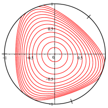
a) b) c)

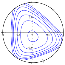
Figure 7: Gravitational three-body problem: contours $-\sqrt{2n}$, $n=1,\ldots,20$, of the functions $\sqrt{\tilde{M}_{k}}\,\tilde{V}$ defined in (66) with $k=1$ (a), $k=2$ (b) and $k=3$ (c). The contours are shown on the shape space $\tilde{\mathcal{Q}}$ represented as the projection of the upper hemisphere of the unit sphere in the $(w_{1},w_{2},w_{3})$-space projected to the unit disk in the $(w_{1},w_{2})$-plane. The ticks on the boundary mark the double collisions (see the main text).

In the different panels in Figs. 8 and 9 we show the projection of the Hill region to the shape space following the colouring procedure described at the end of Sec. 5 for a representative values of $\nu$. The pictures are obtained from the superposition of the shape space contours of the functions $\sqrt{\tilde{M}_{k}}\tilde{V}$, $k=1,2,3$ in (66) for the value of $\nu$ under consideration and colouring the regions enclosed by the contours using the colour code in Fig. 5. We start with large values of $\nu$. For $\nu>\nu_{\text{collinear}\,9}$, there is a simply connected dark grey shaded region corresponding to points for which the accessible region on the orientation sphere is empty, i.e. these shapes do not belong to the Hill region. This dark shaded region ‘spills out’ of the shape space at three places. Attached to the dark grey shaded region are three blue strips where the accessible regions on the orientation sphere are two caps for every point inside. Attached to these regions are the three red regions where for each point inside this region the accessible region on the orientation sphere is a ring. Each of these red regions contains one double collision on its boundary. For large values of $\nu$ (i.e. low energy and/or large values of the magnitude of the angular momentum) the accessible region on the shape space consists of three disconnected components where either component corresponds to one pair of bodies that are close to each other and the third body cannot close to this pair.

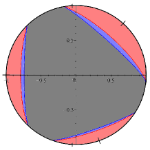
a) b) c)

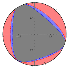
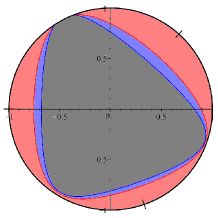
d) e) f)

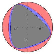
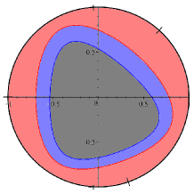
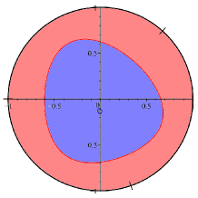
g) h) i)

Figure 8: Gravitational three-body problem: projections of the Hill regions to the shape space for specific values of $\nu$: $\nu>\nu_{\text{collinear}\,9}$ (a), $\nu=\nu_{\text{collinear}\,9}$ (b), $\nu_{\text{collinear}\,9}>\nu>\nu_{\text{collinear}\,8}$ (c), $\nu=\nu_{\text{collinear}\,8}$ (d), $\nu_{\text{collinear}\,8}>\nu>\nu_{\text{collinear}\,7}$ (e), $\nu=\nu_{\text{collinear}\,7}$ (f), $\nu_{\text{collinear}\,7}>\nu>\nu_{\text{Lagrange}\,6}$ (g), $\nu=\nu_{\text{Lagrange}\,6}$ (h), and $\nu_{\text{Lagrange}\,6}>\nu>\nu_{\text{diabolic}\,5}$ (i). The contours are shown on the shape space $\tilde{\mathcal{Q}}$ represented in the same way as in Fig. 7.

When $\nu$ decreases below the values $\nu_{\text{collinear}\,9}$, $\nu_{\text{collinear}\,8}$ and $\nu_{\text{collinear}\,7}$ the dark grey shaded region successfully detaches from the boundary of the shape space such that for $\nu_{\text{Lagrange}\,6}<\nu<\nu_{\text{collinear}\,7}$ the dark shaded region is completely contained in the interior of the shape space and the red region has successively become connected. At all instances a blue region is located between the dark grey region and the red region. Recall that on the boundary of the shape space which corresponds to collinear configurations the principal moments of inertia $\tilde{M}_{2}$ and $\tilde{M}_{3}$ are equal (and $\tilde{M}_{1}=0$). This is why the red and the blue contours detach from the boundary of the shape space simultaneously in Fig. 7 and why the blue strips in Fig. 8 join at $\nu_{\text{collinear}\,9}$, $\nu_{\text{collinear}\,8}$ and $\nu_{\text{collinear}\,7}$ in the observed way.

j) k) l)

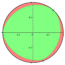
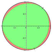
m) n) o)

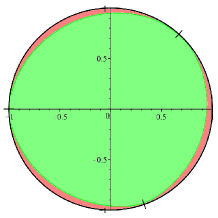
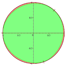
p) q) r)

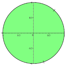
Figure 9: Gravitational three-body problem: continuation of Fig. 8 with values of $\nu$ chosen according to $\nu=\nu_{\text{diabolic}\,5}$ (j), $\nu_{\infty\,4}>\nu>\nu_{\text{diabolic}\,5}$ (k), $\nu=\nu_{\infty\,4}$ (l), $\nu_{\infty\,3}>\nu>\nu_{\infty\,4}$ (m), $\nu=\nu_{\infty\,3}$ (n), $\nu_{\infty\,2}>\nu>\nu_{\infty\,3}$ (o), $\nu=\nu_{\infty\,2}$ (p), $\nu_{\infty\,2}>\nu>\nu_{1}=0$ (q), and $\nu_{1}=0\geq\nu$ (r).

When $\nu$ decreases to $\nu_{\text{Lagrange}\,6}$ from above the dark grey region shrinks to a point which for the present choice of masses is close to but not at $(w_{1},w_{2},w_{3})=(0,0,1)$ and for $\nu<\nu_{\text{Lagrange}\,6}$ it has vanished. The Hill region (projected to the shape space) is hence simply connected for $\nu<\nu_{\text{Lagrange}\,6}$.

The blue region is simply connected for $\nu_{\text{diabolic}\,5}<\nu<\nu_{\text{Lagrange}\,6}$. When $\nu$ decreases to $\nu_{\text{diabolic}\,5}$ the blue region shrinks to a point at $(w_{1},w_{2},w_{3})=(0,0,1)$, and when $\nu$ decreases below $\nu_{\text{diabolic}\,5}$ a simply connected green region grows out of this point. For every point in the green region any point on the orientation sphere is accessible. The unusual bifurcation at $\nu=\nu_{\text{diabolic}\,5}$ observed in the projection to the shape space can be understood from noticing that the graphs of the functions (66) over the shape space give for $k=1$ and $k=2$ a continuously distorted version of the double cone in Fig. 3. When the value of $\nu$ passes through $\nu_{\text{diabolic}\,5}$ the sublevel sets of the functions (66) shown in Figs. 8i-9k are continous deformations of the sublevel sets of a height function in Fig. 3.

For $\nu_{\infty\,4}<\nu<\nu_{\text{diabolic}\,5}$, the green region is completely contained in the interior of the shape space. When $\nu$ takes the values $\nu_{\infty\,4}$, $\nu_{\infty\,3}$ and $\nu_{\infty\,2}$ the green region successively starts to touch the boundary of the shape space at the double collision points. The manifestation of the bifurcations due to critical points at infinity in terms of the sublevel sets touching the boundary at the double collision points can be understood from noticing that a critical point at infinity involves one co-rotating pair of two bodies with the third body at rest at infinity. After scaling such a configuration by the dilation transformation such that the polar moment of inertia $I$ becomes $1$ the co-rotating pair appears to collide.

At $\nu=\nu_{1}=0$ the green region fills the full shape space. This remains to be the case for any $\nu\leq 0$.

As the bifurcation scenario is partly difficult to see in Fig. 9 we show in Fig. 10 the corresponding contours of the function $\sqrt{\tilde{M}_{1}}\,\tilde{V}$ in the $(\chi,\psi)$-plane, $0\leq\chi\leq 2\pi$, $0\leq\psi\leq\pi/2$.

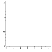
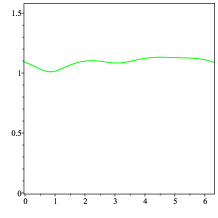
j) k) l)

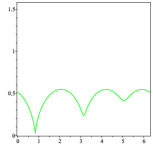
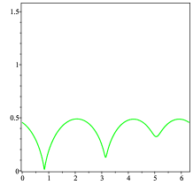
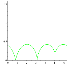
m) n) o)

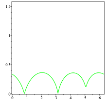
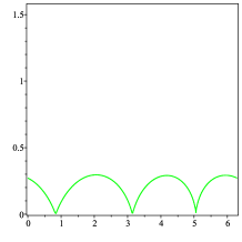
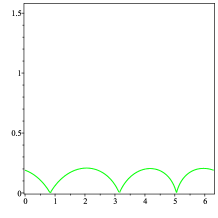
p) q) r)

Figure 10: Gravitational three-body problem: contours of the function $\sqrt{\tilde{M}_{1}}\,\tilde{V}$ in the $(\chi,\psi)$-plane, $0\leq\chi\leq 2\pi$, $0\leq\psi\leq\pi/2$, for the same values of $\nu$ as in the corresponding panels in Fig. 9.

We note that bifurcations observed in Figs. 7 and 9 agree with similar figures shown in [2].

7.2 Helium

We here consider the helium atom as a charged three-body system consisting of two electrons and a nucleus that interact via Coulomb forces. Using atomic units the electrons have masses $m_{1}=m_{2}=1$, the nucleus has mass $m_{3}=7\,289.56$. The electron both have charge -1. The nucleus has charge $+2$. The coefficients in the potential (16) are then $\alpha_{1}=\alpha_{2}=2$ and $\alpha_{3}=-1$.

In Fig. 11 we show again the contours of the functions $\sqrt{\tilde{M}_{k}}\,\tilde{V}$, $k=1,2,3$, defined in (66) analogously to Fig. 7 for the gravitational case. The collision of particles 1 and 2 (two electrons) occurs at a polar angle of about $89.99214109^{\circ}$ and of particles 2 and 3 (electron and nucleus) at a polar angle of about $-0.01571780034^{\circ}$ (see (29) and (30)). The collision of particles 1 and 3 (again electron and nucleus) is located at $180^{\circ}$. As the double collision are close to the coordinate axes in Fig. 11 we do not mark them by special ticks. The potential $\tilde{V}$ is $-\infty$ at the collisions of either of the electrons with the nucleus (polar angles $-0.01571780034^{\circ}$ and $180^{\circ}$) and $+\infty$ at the collisions of the two electrons (polar angle $89.99214109$).

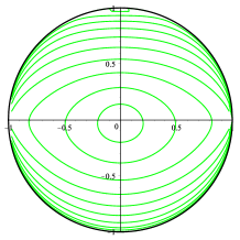
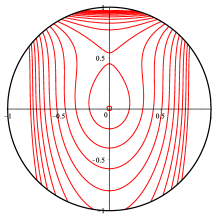
a) b) c)

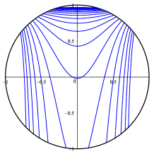
Figure 11: Helium: Contours $-n/3$ for $n=1,\ldots,20$, of the functions $\sqrt{\tilde{M}_{k}}\,\tilde{V}$ defined in (66) with $k=1$ (a), $k=2$ (b) and $k=3$ (c). The presentation is analogously to Fig. 7.

From the contours in Fig. 11 we conclude that there are together with the critical value $\nu_{1}=0$ (where $\nu_{1}=0$ is further commented on in the discussion of Fig. 12 below) in total 5 critical values of $\nu$ resulting from the following events.

• The contours of $\sqrt{\tilde{M}_{1}}\tilde{V}$ touch/detach from the boundary of the shape space (see Fig. 11(a)). This happens simultaneously at both of the double collision points of the electrons with the nucleus.

• $\sqrt{\tilde{M}_{1}}\tilde{V}$ and $\sqrt{\tilde{M}_{1}}\tilde{V}$ simultaneously have a critical point at the center of the unit disk in the $(w_{1},w_{2})$-plane (see Fig. 11(a) and (b)).

• $\sqrt{\tilde{M}_{1}}\tilde{V}$ has a critical point close to the positive $w_{2}$-axis away from the center of the unit disk in the $(w_{1},w_{2})$-plane (see Fig. 11(b)).

• The contours of $\sqrt{\tilde{M}_{2}}\tilde{V}$ and $\sqrt{\tilde{M}_{3}}\tilde{V}$ touch/detach from the boundary of the shape space at polar angle $-120^{\circ}$ (see Figs. 13(b) and (c)). This again happens for the same value of $\nu$ as $\sqrt{\tilde{M}_{2}}\tilde{V}$ and $\sqrt{\tilde{M}_{3}}\tilde{V}$ agree on the boundary of the shape space (i.e. for collinear configurations).

These events can be related to the following nontrivial critical values of $\nu$. Event (i) is a result of the two symmetry related critical points at infinity where either of the electrons is co-rotating with the nucleus and the other electron is at rest with an infinite distance in between. The corresponding value of $\nu$ can be computed from (99). For the helium nucleus and one electron, this gives

$$\nu_{\infty\,2}\approx 1.999725672\,.$$ (101)

Event (ii) results from the diabolic point of the moment of inertia tensor. For the helium system, the corresponding value of $\nu$ can be computed from (97) to be

$$\nu_{\text{diabolic}\,3}\approx 5.420669550\,.$$ (102)

Event (iii) is caused by a non-collinear relative equilibrium involving rotation about the middle principal axis. This is the Langmuir orbit discussed in Sec. 6.1.2. For systems like the helium atom where $\alpha_{2}/\alpha_{3}=-2$, (95) reduces to

$$\nu_{\text{Langmuir}}=\left(\frac{3}{2}\right)^{3}\mu\alpha_{3}^{2}$$ (103)

giving for helium

$$\nu_{\text{Langmuir}\,4}\approx 6.748148600\,.$$ (104)

Event (iv) results from the relative equilibrium associated with the collinear central configuration with the nucleus located in the middle between the two electrons. For the symmetric case with particle $m_{3}$ in the middle, $m_{1}=m_{2}$ and $\alpha_{1}=\alpha_{2}$, the value of $\nu$ in (98) reduces to

$$\nu_{\text{collinear}}=\frac{1}{4}m_{1}(4\alpha_{1}+\alpha_{3})^{2}\,.$$ (105)

Filling in the values of helium gives

$$\nu_{\text{collinear}\,5}=\frac{49}{4}=12.25\,.$$ (106)

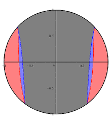
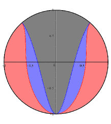
a) b) c)

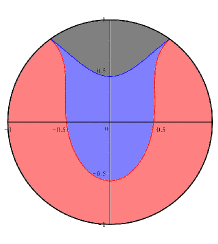
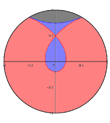
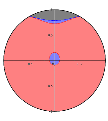
d) e) f)

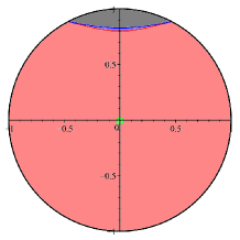
g) h) i)

j) k)

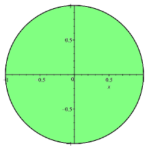
Figure 12: Helium: projections of the Hill regions to the shape space for specific values of $\nu$: $\nu>\nu_{\text{collinear}\,5}$ (a), $\nu=\nu_{\text{collinear}\,5}$ (b), $\nu_{\text{collinear}\,5}>\nu>\nu_{\text{Langmuir}\,4}$ (c), $\nu=\nu_{\text{Langmuir}\,4}$ (d), $\nu_{\text{Langmuir}\,4}>\nu>\nu_{\text{diabolic}\,3}$ (e), $\nu=\nu_{\text{diabolic}\,3}$ (f), $\nu_{\text{diabolic}\,3}>\nu>\nu_{\infty\,2}<$ (g), $\nu=\nu_{\infty\,2}$ (h), $\nu_{\infty\,2}>\nu>\nu_{1}=0$ (i), $\nu=\nu_{1}=0$ (j), and $\nu_{1}=0\geq\nu$. The contours are shown on the shape space $\tilde{\mathcal{Q}}$ represented in the same way as in Fig. 13.

In the different panels in Fig. 12 we again show the projection of the Hill regions to the shape space. The presentation and coulor code is the same as in Figs. 8 and 9 for the gravitational case. We again start with large values of $\nu$. When $\nu$ crosses the value $\nu_{\text{Langmuir}\,4}$ of the Langmuir relative equilibrium a blob detaches from the blue region. At $\nu_{\text{diabolic}\,3}$ the blue blob shrinks to a point and similar to the analogous scenario in the gravitational case a green region grows out of this region when $\nu$ decreases below $\nu_{\text{diabolic}\,3}$. The green region then grows and reaches the boundary of the shape space for the first time at the two double collision points of the nucleus with either of the electrons when $\nu=\nu_{\infty\,2}$. When $\nu$ decreases further to $\nu_{1}=0$ the green region grows until the red and blue regions have vanished at $\nu_{1}=0$. A grey forbidden region near the double collision of the electrons remains at $\nu_{1}=0$. This is due to the potential energy going to plus infinity at the double collision of the two electrons. This is different from the gravitational case where the forces between the bodies is always attractive. However, like in any charged three-body system for every shape, any orientation is possible for $\nu<\nu_{1}=0$ (i.e. for positive total energies $E$), see Theorem 5.1.

7.3 Compound of two electrons and one positron

In the following we consider a system of two electrons e^- and one positron e⁺ interacting via Coulomb forces. In atomic units, e^- has charge -1 and mass 1. The positron e⁺ has the same mass but opposite charge. The two electrons are labeled 1 and 2. The positron is assigned the label 3. The coefficients in the potential (16) are then $\alpha_{1}=\alpha_{2}=1$ and $\alpha_{3}=-1$.

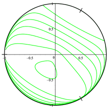
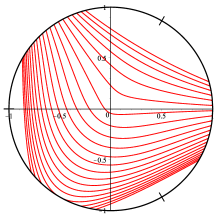
a) b) c)

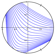
Figure 13: Compound of two electrons and one positron: contours $-n/8$, $n=1,\ldots,20$, of the functions $\sqrt{\tilde{M}_{k}}\,\tilde{V}$ defined in (66) with $k=1$ (a), $k=2$ (b) and $k=3$ (c). The presentation is analogously to Fig. 7.

In Fig. 13 we show the contours of the functions $\sqrt{\tilde{M}_{k}}\,\tilde{V}$, $k=1,2,3$, defined in (66) analogously to Fig. 7 for the gravitational case. For equal masses, the double collision of particles 1 and 2 (two electrons) occurs at a polar angle of $60^{\circ}$ and of particles 2 and 3 (electron and positron) at angle $-60^{\circ}$ (see (29) and (30)). The collision of particles 1 and 3 (again electron and positron) is located at $180^{\circ}$. The potential $\tilde{V}$ is $-\infty$ at the collisions of either of the electrons with the positron (polar angles $-60^{\circ}$ and $180^{\circ}$) and $+\infty$ at the collisions of the two electrons (polar angle $60^{\circ}$).

From the contours in Fig. 13 we conclude that together with the critical value $\nu_{1}=0$ there are four critical values for $\nu$ caused by the following events.

• The contours of $\sqrt{\tilde{M}_{1}}\tilde{V}$ touch/detach from the boundary of the shape space (see Fig. 13(a)). This happens simultaneously at both of the symmetric double collisions points of the electrons with the positron.

• $\sqrt{\tilde{M}_{1}}\tilde{V}$ has a critical point in the interior of the the shape space (see Fig. 13(a)).

• The contours of $\sqrt{\tilde{M}_{2}}\tilde{V}$ and $\sqrt{\tilde{M}_{3}}\tilde{V}$ touch/detach from the boundary of the shape space at polar angle $-120^{\circ}$ (see Figs. 13(b) and (c)). This happens for the same value of $\nu$ as $\sqrt{\tilde{M}_{2}}\tilde{V}$ and $\sqrt{\tilde{M}_{3}}\tilde{V}$ agree on the boundary of the shape space (i.e. for collinear configurations).

As discussed for the previous two examples event (i) can be related to critical points at infinity. Like in the case of helium there are two symmetry related critical points at infinity corresponding to a co-rotating electron positron pair and a resting second electron with an infinite distance in between. The corresponding value of the bifurcation parameter is

$$\nu_{\infty\,2}=\frac{1}{4}=0.25\,.$$ (107)

As a result of the equal masses and absolute values of the charges in the electron-electron-positron compound, it happens that the value of the bifurcation parameter corresponding to the diabolic point of the moment of inertia tensor gives the same value, i.e.

$$\nu_{\text{diabolic}\,2}=\nu_{\infty\,2}.$$ (108)

The event (ii) results from a non-collinear relative equilibrium involving rotation about the first principal axis. This relative equilibrium is again a Langmuir orbit and the corresponding value of $\nu$ can be calculated from (95) to be

$$\nu_{\text{Langmuir}\,3}\approx 0.2925594730\,.$$ (109)

Similarly to the helium case, event (iii) can be related to the collinear central configuration where the positron is located right between the two electrons on a line. The corresponding value of $\nu$ can be calculated from the symmetric version of (98) in (105) to give

$$\nu_{\text{collinear}\,4}=\frac{9}{4}=2.25.$$ (110)

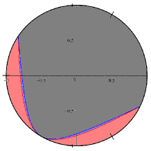
a) b) c)

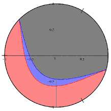
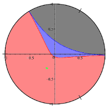
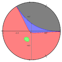
d) e) f)

g) h) i)

Figure 14: Compound of two electrons and one positron: projections of the Hill regions to the shape space for specific values of $\nu$: $\nu>\nu_{\text{collinear}\,4}$ (a), $\nu=\nu_{\text{collinear}\,4}$ (b), $\nu_{\text{collinear}\,4}>\nu>\nu_{\text{Langmuir}\,3}$ (c), $\nu=\nu_{\text{Langmuir}\,3}$ (d), $\nu_{\text{Langmuir}\,3}>\nu>\nu_{\infty\,2}=\nu_{\text{diabolic}\,2}$ (e), $\nu=\nu_{\infty\,2}=\nu_{\text{diabolic}\,2}$ (f), $\nu_{\infty\,2}=\nu_{\text{diabolic}\,2}>\nu>\nu_{1}=0$ (g), $\nu=\nu_{1}$ (h), and $\nu_{1}=0>\nu$ (i). The contours are shown on the shape space $\tilde{\mathcal{Q}}$ represented in the same way as in Fig. 13.

In the different panels in Fig. 14 we again show the projections of the Hill regions to the shape space for representative values of $\nu$. The presentation and colour code is again the same as in Figs. 8 and 9 for the gravitational case. Starting with large values of $\nu$ there is for $\nu>\nu_{\text{collinear}\,4}$ a grey region not belonging to the Hill region that separates the accessible part of the shape space into two disconnected components. For points in the two red components, the accessible region on the orientation sphere is a ring. These two components contain on their boundary the double collisions where one of the electrons collides with the positron. The forbidden region has the double collision of the electrons as a boundary point. Between the grey region and the red regions there are blue strips where the accessible region on the orientation sphere consists of two caps. At $\nu=\nu_{\text{collinear}\,4}$ the boundary of the grey regions and the blue region are tangental to the boundary of the shape space at the point corresponding to the collinear central configuration which has polar angle $-120^{\circ}$ in the $(w_{1},w_{2})$-plane. For $\nu<\nu_{\text{collinear}\,4}$ the Hill region is simply connected. For $\nu_{\text{Langmuir}\,3}<\nu<\nu_{\text{collinear}\,4}$, the blue and the red regions are both simply connected. At $\nu=\nu_{3}$ a green dot emerges in the red region because of which the red region is no longer simply connected for $\nu<\nu_{\text{Langmuir}\,3}$. This green dot results from the non-collinear relative equilibrium given by the Langmuir orbit which corresponds to rotation about the first principal axis. When $\nu$ decreases from $\nu_{\text{Langmuir}\,3}$ to $\nu_{\text{diabolic}\,2}=\nu_{\infty\,2}$ the green region grows until it touches the boundary of the shape space for the first time at the two electron-electron double collision points for $\nu=\nu_{\text{diabolic}\,2}=\nu_{\infty\,2}$. Whereas this is due to the two symmetry related critical points at infinity, simultaneously for the same value of $\nu$, the green and the blue region touch at the center of the unit disk in the $(w_{1},w_{2})$-plane where the smallest and the middle principal moments of inertia are equal. At the point where they touch the boundaries of the green and blue regions are not smooth. When $\nu$ decreases below $\nu_{\text{diabolic}\,2}=\nu_{\infty\,2}$ the green and the blue region detach again and the corners on their boundaries vanish again. This scenario is different from the scenarios resulting from the diabolic point in the previous two examples. In the previous two examples we explained the scenarios from noticing that the graphs of the functions (66) over the shape space give for $k=1$ and $k=2$ a distorted version of the double cone in Fig. 3. In the present case the double cone is distorted in such a way that the boundaries of the sublevel sets have the topology of the intersections of the double cone with vertical planes in Fig. 3 (as opposed to horizontal planes like in the gravitational case and in the helium atom). When the value of $\nu$ passes through $\nu_{\text{diabolic}\,5}$ the sublevel sets of the functions (66) then lead to the bifurcation shown in Figs. 14e-14g. Upon $\nu$ approaching $\nu_{1}=0$ from above the red and the blue regions are shrinking due to the growing green region until at $\nu=\nu_{1}=0$ both the red region and the blue regions have vanished. Similar to the case of the helium atom and unlike the gravitational case there remains a forbidden region near the point of the electron-electron collision at polar angle $60^{\circ}$. For $\nu<\nu_{1}=0$, the full shape space belongs to the Hill region and, as in every charged three-body system, for every shape, every orientation is possible (see Theorem 5.1).

8 Discussion and outlook

The study of the Hill region of the gravitational three-body problem has a long history. It has been, e.g., the subject of the famous and by now disproved Birkhoff conjecture stating that all bifurcations of Hill regions are related to central configurations (see the discussion in [2]). In the present paper we studied the more general case of charged three-body systems which include the gravitational system as a special case. As shown in [1], charged three-body systems can have relative equilibria which do not project to central configurations. It is therefore even more elusive to expect the Birkhoff conjecture to hold in the case of charged three-body problems. In this paper we provided two examples of systems which have relative equilibria that do not project to central configurations. In both examples the relative equilibrium is given by the Langmuir orbit. In fact we conjecture that for charged three-body systems the only possible non-collinear relative equilibria are the Lagrange type relative equilibria familiar from the gravitational case which, as stated in this paper, are expected to exist more generally for purely attractive inter-body forces and the Langmuir type relative equilibria for systems with coexisting attractive and repulsive inter-body forces. In a charged three-body system the Lagrange and the Langmuir type relative equilibria cannot coexist. It is also possible that a charged-three body problem has no non-collinear relative equilibria at all (e.g. if all inter-body forces are repulsive).

In [2] the Hill regions are also used to study the topology of the integral manifolds. It would be interesting to generalise such results to the charged case. The present paper provides first steps in this direction. We however point out again that the symplectic reduction used in this paper to define the Hill regions is singular for collinear configurations. A study of the topology of the integral manifolds for the charged case in a similar fashion as in [2] would hence require a more careful analysis of the boundary of the shape space to which the collinear configurations project. In the present paper we have given an explanation of the pseudo critical point which leads to the seeming bifurcation of the Hill regions observed when projecting these to the shape space by relating this seeming bifurcation to the diabolic point of the moment of inertia tensor.

Our future studies motivated by the present paper and the preceding two papers [1, 3] concern the stability of relative equilibria and the existence of the Langmuir type relative equilibria also for less symmetric systems than the helium atom and the electron-electron-positron compound studied in the present paper. Both of these items are of importance for the final goal to determine the topology of the integral manifolds for charged three-body systems in full generality.

References

- [1] I. Hoveijn, H. Waalkens, and M. Zaman. Critical points of the integral map of the charged three-body problem. Indagationes Mathematicae, 30(1):165–196, 2019.
- [2] C.K. McCord, K.R. Meyer, and Q. Wang. The Integral Manifolds of the Three Body Problem. Number no. 628 in American Mathematical Society: Memoirs of the American Mathematical Society. American Mathematical Society, 1998.
- [3] I. Hoveijn, H. Waalkens, and M. Zaman. Critical points at infinity in charged -body systems. submitted, 2021.
- [4] R. G. Littlejohn and M. Reinsch. Gauge fields in the separation of rotations and internal motions in the -body problem. Rev. Mod. Phys., 69:213–275, 1997.
- [5] Patrick Cornille. Advanced electromagnetism and vacuum physics. World Scientific, River Edge, N.J, 2003.
- [6] Ü. Çiftçi and H. Waalkens. Phase space structures governing reaction dynamics in rotating molecules. Nonlinearity, 25:791–892, 2012.
- [7] Ü. Çiftçi, H. Waalkens, and H. W. Broer. Cotangent bundle reduction and Poincaré-Birkhoff normal forms. Physica D, 268:1–13, 2014.
- [8] I. N. Kozin, R. M. Roberts, and J. Tennyson. Relative equilibria of D2H+ and H2D+. Molecular Physics, 98:295–307, 2000.
- [9] T. Iwai and H. Yamaoka. Stratified reduction of classical many-body systems with symmetry. J. Phys. A, Math. Gen., 38:2415–2439, 2005.
- [10] R. Moeckel. Lecture notes on celestial mechanics especially central configuration. Trieste, Italy in October 1994.
- [11] A. Guichardet. On rotation and vibrationsmotions of molecules. Annales de l’I.H.P., section A, 40(3):329–342, 1984.
- [12] R. Clausius. XVI. On a mechanical theorem applicable to heat. Philosophical Magazine Series 4, 40(265):122–127, 1870.
- [13] J.M.A. Danby. Fundamentals of celestial mechanics. Willmann-Bell, Richmond, Virginia, 1992.
- [14] I. Langmuir. The structure of the helium atom. Science, 51(1329):605–607, 1920.
- [15] C. Simo. El conjunto de bifurcacion en el problema espacial de tres cuerpos. In Acta I Asamblea Nacional de Astronomia y Astrofisica, pages 211–217. Instituto de Astrofisica, Univ. de la Laguna, Spain, 1975.
- [16] Donald G. Saari. From rotations and inclinations to zero configurational velocity surfaces i. a natural rotating coordinate system. Celestial mechanics, 33(4):299–318, 1984.
- [17] Donald G. Saari. From rotations and inclinations to zero configurational velocity surfaces, ii. the best possible configurational velocity surfaces. Celestial mechanics, 40(3):197–223, 1987.
- [18] D.G. Saari. Symmetry in n-particle systems. In K.R. Meyer and D.G. Saari, editors, Hamiltonian Dynamical Systems, Proceedings of a Summer Research Conference held June 21-27, 1987, pages 23–42.