Clustering with fair-center representation: parameterized approximation algorithms and heuristics

Abstract.

We study a variant of classical clustering formulations in the context of algorithmic fairness, known as diversity-aware clustering. In this variant we are given a collection of facility subsets, and a solution must contain at least a specified number of facilities from each subset while simultaneously minimizing the clustering objective ($k$-median or $k$-means). We investigate the fixed-parameter tractability of these problems and show several negative hardness and inapproximability results, even when we afford exponential running time with respect to some parameters.

Motivated by these results we identify natural parameters of the problem, and present fixed-parameter approximation algorithms with approximation ratios $\big{(}1+\frac{2}{e}+\epsilon\big{)}$ and $\big{(}1+\frac{8}{e}+\epsilon\big{)}$ for diversity-aware $k$-median and diversity-aware $k$-means respectively, and argue that these ratios are essentially tight assuming the gap-exponential time hypothesis. We also present a simple and more practical bicriteria approximation algorithm with better running time bounds. We finally propose efficient and practical heuristics. We evaluate the scalability and effectiveness of our methods in a wide variety of rigorously conducted experiments, on both real and synthetic data.

1. Introduction

Consider the problem of forming a representative committee. In essence, the task amounts to finding a group of people among a given set of candidates, to represent the will of a (usually) larger body of constituents. In computational terms, this can be modeled as a clustering problem like $k\text{\sc{-Median}}$: each cluster center is a chosen candidate, and the points in the corresponding cluster are the constituents it best represents.

In certain scenarios, it may be adequate to consider additional requirements. For instance, it may be necessary that at least a number of the chosen committee members belong to a certain minority-ethnic background, to ensure that all groups in a society are represented in the decision-making process. This problem was recently formalized as the diversity-aware $k$-median problem ($\text{\sc Div-}k\text{\sc-Med}$) (Thejaswi et al., 2021b). As in conventional $k\text{\sc{-Median}}$, the goal is to pick $k$ facilities to minimize the sum of distances from clients to their closest facility (Arya et al., 2001). In $\text{\sc Div-}k\text{\sc-Med}$, however, each facility is associated to an arbitrary number of attributes from a given finite set. The solution is required to contain at least a certain number of facilities having each attribute (the requirement for each attribute is given to us as part of the input).

Thejaswi et al. showed that this additional constraint makes $k\text{\sc{-Median}}$ harder to solve (Thejaswi et al., 2021b), in the following sense. While $k\text{\sc{-Median}}$ is $\mathbf{NP}$-hard to solve exactly, it is $\mathbf{NP}$-complete to even decide whether a $\text{\sc Div-}k\text{\sc-Med}$ instance has a feasible solution. The rest of their work, thus, focuses on tractable cases and practical heuristics. This work follows a recent line of interest in algorithmic fairness, which has attracted significant attention in recent years. In the design of fair algorithms, additional constraints are imposed on the objective function to ensure equitable —or otherwise desirable— outcomes for the different groups present in the data (Zafar et al., 2017; Dwork et al., 2018; Chierichetti et al., 2017; Schmidt et al., 2019; Huang et al., 2019; Backurs et al., 2019; Bercea et al., 2019).

Contributions. In this paper we provide a much more comprehensive analysis of $\text{\sc Div-}k\text{\sc-Med}$ ($\text{\sc Div-}k\text{\sc-Means}$ resp.), addressing computational complexity, approximation algorithms, and practical heuristics for the problems. In particular, we give the first known and tight approximation results for the problems.

Since we know that $\text{\sc Div-}k\text{\sc-Med}$ does not admit polynomial-time approximation algorithms (Thejaswi et al., 2021b), we first focus on fixed-parameter tractability (Cygan et al., 2015). That is, we seek to answer the following question: can we hope to find algorithms with approximation guarantees by allowing their running time to be exponential in some input parameter? In other words, is approximating $\text{\sc Div-}k\text{\sc-Med}$ ($\text{\sc Div-}k\text{\sc-Means}$ resp.) fixed-parameter tractable (FPT)?

Our main result in this paper is a positive answer to this question. We give a constant-factor approximation algorithm with running time parameterized by $k$ and $t$, the number of clusters and the number of candidate attributes respectively. We further develop our understanding of $\text{\sc Div-}k\text{\sc-Med}$ ($\text{\sc Div-}k\text{\sc-Means}$ resp.) by characterizing the problem in terms of parameterized complexity. Finally, we consider practical aspects of the problem and design effective, practical heuristics which we evaluate through a variety of experiments. Our contributions are summarized below:

Computational complexity. We strengthen the known complexity results for $\text{\sc Div-}k\text{\sc-Med}$ ($\text{\sc Div-}k\text{\sc-Means}$ resp.) by analyzing its parameterized complexity and inapproximibility. In particular, for these problems,

• we give a lower bound for the running time of optimal and approximation algorithms (Corollary 3.1);

• we show that finding bicriteria approximation algorithms is fixed-parameter intractable with respect to the number of clusters (Proposition 3.2);

• we show that they are fixed-parameter intractable with respect to various choices of parameters (Proposition 3.3).

Approximation algorithms.

• We give the first and tight fixed-parameter tractable constant-factor approximation algorithm for $\text{\sc Div-}k\text{\sc-Med}$ ($\text{\sc Div-}k\text{\sc-Means}$ resp.) w.r.t. $k$ and $t$ (Theorem 4.1).

• We give a faster and tight dynamic programming algorithm for deciding the feasibility (Theorem 6.1). This yields a faster bicriteria approximation algorithm (Theorem 4.2).

Practical heuristics and empirical evaluation.

• Despite their theoretical guarantees, the methods discussed above are impractical. We propose a practical approach to find feasible solutions based on linear programming. Despite its lack of guarantees, we show how it can be used as a building block in the design of effective heuristics.

• We evaluate the proposed methods in a wide variety of experimental results, rigorously conducted on real an synthetic datasets. In particular, we show that the proposed heuristics are able to reliably and efficiently find feasible solutions of good quality on a variety of real data sets.

The rest of the paper is organized as follows. In Section 2 we introduce notation and basic notions. In Section 3 we present our computational complexity analysis, and Section 4 gives an overview of our main results. Our algorithms are described in Sections 5 and  6, and our experimental results in Section 7. An overview of related work is given in Section 8, while Section 9 provides concluding remarks. Some proofs are deferred to the Supplementary.

2. Preliminaries

In this section we introduce notation and problem definitions.

Notation. Given a metric space $(U,d)$, a set $C\subseteq U$ of clients, a set $F\subseteq U$ of facilities and a subset $S\subseteq F$ of facilities, we denote by $\text{\sf cost}(S)=\sum_{c\in C}d(c,S)$ the clustering cost of $S$, where $d(c,S)=\min_{s\in S}d(c,s)$. We say that $C$ is weighted when every $c\in C$ is associated to a weight $w_{c}\in\mathbb{R}$, and the clustering cost becomes $\text{\sf cost}(S)=\sum_{c\in C}w_{c}\cdot d(c,S)$. Similarly, for $C^{\prime}\subseteq C$ and $S\subseteq F$, we write $\text{\sf cost}(C^{\prime},S)=\sum_{c\in C^{\prime}}w_{c}\cdot d(c,S)$. Further, given a collection $\mathscr{G}=\{G_{1},\dots,G_{t}\}$ of facility groups such that $G_{i}\subseteq F$, for each facility $f\in F$ we denote by $\vec{\chi}_{f}\in\{0,1\}^{t}$ the characteristic vector of $f$ with respect to $\mathscr{G}$, and is defined as $\vec{\chi}_{f}[i]=1$ if $f\in G_{i}$, $0$ otherwise, for all $i\in[t]$. For $\eta>0$ and $a\in\mathbb{Z}_{\geq 0}$, we denote $[a]_{\eta}\in\mathbb{Z}$ as the smallest integer such that $(1+\eta)^{[a]_{\eta}}\geq a$. For a metric space $(U,d)$, the aspect ratio is defined as $\Delta=\frac{\max_{x,y\in U}d(x,y)}{\min_{x,y\in U}d(x,y)}$.

In this paper we use standard parameterized complexity terminology from Cygan et al. (Cygan et al., 2015).

Definition 2.1 (Diversity-aware $k$-median ($\text{\sc Div-}k\text{\sc-Med}$)).

Given a metric space $(U,d)$, a set $C\subseteq U$ of clients, a set $F\subseteq U$ of facilities, a collection, called groups, $\mathscr{G}=\{G_{1},\dots,G_{t}\}$of facility sets $G_{i}\subseteq F$, a budget $k\leq|F|$, and a vector of requirements $\vec{r}=(r[1],\dots,r[t])$. The problem asks to find a subset of facilities $S\subseteq F$ of size $k$, satisfying $|S\cap G_{i}|\geq r[i]$ for all $i\in[t]$, such that the clustering cost of $S$, $\text{\sf cost}(S)=\sum_{c\in C}d(c,S)$ is minimized. An instance of $\text{\sc Div-}k\text{\sc-Med}$ is denoted as $I=((U,d),F,C,\mathscr{G},\vec{r},k)$.

In diversity-aware $k$-means problem ($\text{\sc Div-}k\text{\sc-Means}$), the clustering cost of $S\subseteq F$ is $\text{\sf cost}(S)=\sum_{c\in C}d(c,S)^{2}$. We denote $r=\max_{i\in[t]}r[i]$ and we assume $\Delta$ is polynomially bounded w.r.t $|U|$ (Cohen-Addad et al., 2019).

3. Hardness

To motivate the choice of parameters for designing FPT algorithms, we characterize the hardness of $\text{\sc Div-}k\text{\sc-Med}$ ($\text{\sc Div-}k\text{\sc-Means}$ resp.) based on standard complexity theory assumptions. Observe that $\text{\sc Div-}k\text{\sc-Med}$ ($\text{\sc Div-}k\text{\sc-Means}$ resp.) problems are an amalgamation of two independent problems: ($i$) finding a subset of facilities $S\subseteq F$ of size $|S|=k$ that satisfies the requirements $|S\cap G_{i}|\geq{r[i]}$ for all $i\in[t]$, and ($ii$) minimizing the $k\text{\sc{-Median}}$ ($k\text{\sc{-Means}}$ resp.) clustering cost. To remain consistent with the problem statement of Thejaswi et al. (Thejaswi et al., 2021b), we refer to subproblem ($i$) as the requirement satisfiability problem (${\vec{r}}\text{\sc{-sat}}$), where the cost of clustering is ignored. If we ignore the requirements in ($i$) we obtain the classical $k\text{\sc{-Median}}$ ($k\text{\sc{-Means}}$ resp.) formulation, which immediately establishes the $\mathbf{NP}$-hardness of $\text{\sc Div-}k\text{\sc-Med}$ ($\text{\sc Div-}k\text{\sc-Means}$ resp.).

A reduction of the vertex cover problem to ${\vec{r}}\text{\sc{-sat}}$ is sufficient to show that $\text{\sc Div-}k\text{\sc-Med}$ ($\text{\sc Div-}k\text{\sc-Means}$ resp.) are inapproximable to any multiplicative factor in polynomial-time even if all the subsets are of size two (Thejaswi et al., 2021a, Theorem 3). The $\mathbf{W[2]}$-hardness of $\text{\sc Div-}k\text{\sc-Med}$ ($\text{\sc Div-}k\text{\sc-Means}$ resp.) with respect to parameter $k$ is a consequence of the fact that $k\text{\sc{-Median}}$ ($k\text{\sc{-Means}}$ resp.) are $\mathbf{W[2]}$-hard, which follow from a reduction by Guha and Kuller (Guha and Khuller, 1998). More strongly, combining the result of (Thejaswi et al., 2021b, Lemma 1) with the strong exponential time hypothesis (SETH) (Impagliazzo and Paturi, 2001), we conclude the following: if we only consider the parameter $k$, a trivial exhaustive-search algorithm is our best hope for finding an optimal, or even an approximate, solution to $\text{\sc Div-}k\text{\sc-Med}$ ($\text{\sc Div-}k\text{\sc-Means}$ resp.). The proof is in Supplementary A.3.

Corollary 3.1.

Assume SETH. For all $k\geq 3$ and $\epsilon>0$, there exists no $\mathscr{O}(|{F}|^{k-\epsilon})$ algorithm to solve $\text{\sc Div-}k\text{\sc-Med}$ ($\text{\sc Div-}k\text{\sc-Means}$ resp.). Furthermore, there exists no $\mathscr{O}(|{F}|^{k-\epsilon})$ algorithm to approximate $\text{\sc Div-}k\text{\sc-Med}$ ($\text{\sc Div-}k\text{\sc-Means}$ resp.) to any multiplicative factor.

Given the $\mathbf{W[2]}$-hardness of $\text{\sc Div-}k\text{\sc-Med}$ with respect to parameter $k$, it is natural to consider relaxations of the problem. An obvious question is whether we can approximate $\text{\sc Div-}k\text{\sc-Med}$ in FPT time w.r.t $k$, if we are allowed to open, say, $f(k)$ facilities instead of $k$, for some function $f$. Unfortunately, this is also unlikely as $\text{\sc Div-}k\text{\sc-Med}$ captures $k\text{\sc-Dom\-Set}$ (Thejaswi et al., 2021b, Lemma 1), and even finding a dominating set of size $f(k)$ is $\mathbf{W[1]}$-hard (S. et al., 2019). The proof is in Supplementary A.3.

Proposition 3.2.

For any function $f(k)$, finding $f(k)$ facilities that approximate the $\text{\sc Div-}k\text{\sc-Med}$ ($\text{\sc Div-}k\text{\sc-Means}$ resp.) cost to any multiplicative factor in FPT time with respect to parameter $k$ is $\mathbf{W[1]}$-hard.

A possible way forward is to identify other parameters of the problem, to design FPT algorithms to solve the problem optimally. As established earlier, $k\text{\sc{-Median}}$ is a special case of $\text{\sc Div-}k\text{\sc-Med}$ when $t=1$. This immediately rules out an exact FPT algorithm for $\text{\sc Div-}k\text{\sc-Med}$ with respect to parameters $(k,t)$. Furthermore, we caution the reader against entertaining the prospects of other, arguably natural, parameters, such as the maximum lower bound $r=\max_{i\in[t]}r[i]$ (ruled out by the relation $r[i]\leq k$) and the maximum number of groups a facility can belong to $\mu=\max_{f\in F}(|{G_{i}}:f\in G_{i},i\in[t]|)$ (ruled out by the relaxation $\mu\leq t$).

Proposition 3.3.

Finding an optimal solution for $\text{\sc Div-}k\text{\sc-Med}$ ($\text{\sc Div-}k\text{\sc-Means}$ resp.) is $\mathbf{W[2]}$-hard with respect to parameters $(k,t)$, $(r,t)$ and $(\mu,t)$.

The above intractability results thwart our hopes of solving the $\text{\sc Div-}k\text{\sc-Med}$ problem optimally in FPT time. We then ask, are there any parameters of the problem that allow us to find an approximate solution in FPT time? We answer this question positively, and present a tight FPT-approximation algorithm w.r.t $(k,t)$, the number of chosen facilities and the number of facility groups.

4. Our results

Our main result, stated below, shows that a constant-factor approximation of $\text{\sc Div-}k\text{\sc-Med}$ ($k\text{\sc{-Means}}$ resp.) can be achieved in FPT time with respect to parameters $(k,t)$. In fact, somewhat surprisingly, the factor is the same as the one achievable for $k\text{\sc{-Median}}$ ($k\text{\sc{-Means}}$ resp.). So despite the stark contrast in their polynomial-time approximability, the FPT landscape is rather similar for these two problems. We also note that under the gap-exponential time hypothesis (Gap-ETH), the approximation ratio achieved in Theorem 4.1 is essentially tight for any FPT algorithm w.r.t $(k,t)$. This follows from combining the fact that the case $t=1$ is essentially $k\text{\sc{-Median}}$ ($k\text{\sc{-Means}}$ resp.) with the results of Cohen-Addad et al. (Cohen-Addad et al., 2019), which assuming Gap-ETH gives a lower bound for any FPT algorithm w.r.t $k$. This bound matches their —and our— approximation guarantee.

Theorem 4.1.

For every $\epsilon>0$, there exists a randomized $(1+\frac{2}{e}+\epsilon)$-approximation algorithm for $\text{\sc Div-}k\text{\sc-Med}$ with time time $f(k,t,\epsilon)\cdot\textsf{poly}(|U|)$, where $f(k,t,\epsilon)=\mathscr{O}\left(\left(\frac{2^{t}k^{3}\log^{2}k}{\epsilon^{2}\log(1+\epsilon)}\right)^{k}\right)$. Furthermore, the approximation ratio is tight for any FPT algorithm w.r.t $(k,t)$, assuming Gap-ETH. For $\text{\sc Div-}k\text{\sc-Means}$, with the same running time, we obtain $(1+\frac{8}{e}+\epsilon)$-approximation, which is tight assuming Gap-ETH.

Finally, in Section 6 we will point out a simple observation: by relaxing the upper bound on the number of facilities to at most $2k$, we can use a practical local-search heuristic and obtain a slightly weaker quality guarantee with better running time bounds. To achieve this we make use of Theorem 6.1.

Theorem 4.2.

For every $\epsilon>0$, there exists a randomized $(3+\epsilon)$-approximation algorithm that outputs at most $2k$ facilities for the $\text{\sc Div-}k\text{\sc-Med}$ problem in time $\mathscr{O}(2^{t}(r+1)^{t}\cdot\textsf{poly}(|U|,1/\epsilon))$.

5. Algorithms

In this section we present an FPT approximation algorithm for $\text{\sc Div-}k\text{\sc-Med}$. For $\text{\sc Div-}k\text{\sc-Means}$, the ideas are similar. Throughout the section, by FPT we imply FPT w.r.t $(k,t)$.

A birds-eye view of our algorithm (see Algorithm 1) is as follows: Given a feasible instance of $\text{\sc Div-}k\text{\sc-Med}$, we first carefully enumerate collections of facility subsets that satisfy the lower-bound requirements (Section 5.1). For each such collection, we obtain a constant-factor approximation of the optimal cost of the collection (Section 5.3). Since at least one of these feasible solutions is optimal, the corresponding approximate solution will be an approximate solution for the $\text{\sc Div-}k\text{\sc-Med}$ problem. A key ingredient for obtaining a constant factor approximation in FPT time is to shrink the set of clients. For this we rely on the notion of coresets (Section  5.2).

In the exposition to follow, we will refer to the problem of $k\text{\sc{-Median}}$ with $p$-partition matroid constraints:

Definition 5.1 ($k\text{\sc{-Median}}$ with $p$-Partition Matroid ($k\text{\sc-Med-}p\text{\sc-PM}$)).

Given a metric space $(U,d)$, a set of clients $C\subseteq U$, a set of facilities $F\subseteq U$ and a collection $\mathscr{E}=\{E_{1},\dots,E_{p}\}$ of disjoint facility groups called a $p$-partition matroid. The problem asks to find a subset of facilities $S\subseteq F$ of size $k$, containing at most one facility from each group $E_{i}$, so that the clustering cost of $S$, $\text{\sf cost}(S)=\sum_{c\in C}d(c,S)$ is minimized. An instance of $k\text{\sc-Med-}p\text{\sc-PM}$ is specified as $J=((U,d),F,C,\mathscr{E},k)$.

5.1. Finding feasible constraint patterns

We start by defining the concept of constraint pattern. Given an instance $I=((U,d),F,C,\mathscr{G},\vec{r},k)$ of $\text{\sc Div-}k\text{\sc-Med}$, where $\mathscr{G}=\{G_{1},\dots,G_{t}\}$, consider the set $\{\vec{\chi}_{f}\}_{f\in F}$ of the characteristic vectors of $F$. For each $\vec{\gamma}\in\{0,1\}^{t}$, let $E(\vec{\gamma})=\{f\in F:{\vec{\chi}}_{f}=\vec{\gamma}\}$ denote the set of all facilities with characteristic vector $\vec{\gamma}$. Finally, let $\mathscr{E}=\{E(\vec{\gamma}):\vec{\gamma}\in\{0,1\}^{t}\}$. Note that $\mathscr{E}$ induces a partition on $F$.

Given a $k$-multiset $\pazocal{E}=\{E(\vec{\gamma}_{i_{1}}),\dots,E(\vec{\gamma}_{i_{k}})\}$, where each $E(\vec{\gamma}_{i_{j}})\in\mathscr{E}$, the constraint pattern associated with $\pazocal{E}$ is the vector obtained by the element-wise sum of the characteristic vectors $\{\vec{\gamma}_{i_{1}},\dots,\vec{\gamma}_{i_{k}}\}$, that is, $\sum_{j\in[k]}\vec{\gamma}_{i_{j}}$. A constraint pattern is said to be feasible if $\sum_{j\in[k]}\vec{\gamma}_{i_{j}}\geq\vec{r}$, where the inequality is taken element-wise.

Lemma 5.2.

Given an instance $I=((U,d),F,C,\mathscr{G},\vec{r},k)$ of $\text{\sc Div-}k\text{\sc-Med}$, we can enumerate all the $k$-multisets with feasible constraint pattern in time $\mathscr{O}(2^{tk}t|U|)$.

Proof.

There are $|\mathscr{E}|+k-1\choose k$ possible $k$-multisets of $\mathscr{E}$, so enumerating all feasible constraint patterns can be done in $\mathscr{O}(|\mathscr{E}|^{k}t)$ time. Further, the enumeration of $\mathscr{E}$ itself can be done in time $\mathscr{O}(2^{t}|F|)$, since $|\mathscr{E}|\leq 2^{t}$. Hence, time complexity of enumerating all feasible constraint patterns is $\mathscr{O}(2^{tk}t|U|)$. ∎

Observe that for every $k$ multiset $\pazocal{E}=\{E(\vec{\gamma}_{i_{1}}),\dots,E(\vec{\gamma}_{i_{k}})\}$ with a feasible constraint pattern, picking an arbitrary facility from each $E(\vec{\gamma}_{i_{j}})$ yields a feasible solution to the $\text{\sc Div-}k\text{\sc-Med}$ instance $I$.

5.2. Coresets

Our algorithm relies on the notion of coresets. The high-level idea is to reduce the number of clients such that the distortion in the sum of distances is bounded to a multiplicative factor $(1\pm\nu)$, for some $\nu>0$. Given an instance $((U,d),C,F,k)$ of the $k\text{\sc-Med-}k\text{\sc-PM}$ problem, for every $\nu>0$ we can reduce the number of clients in $C$ to a weighted set $C^{\prime}$ of size $|C^{\prime}|=\mathscr{O}({\nu}^{-2}k\log|U|)$. We make use of the coreset construction for $k\text{\sc{-Median}}$ by Feldman and Langberg (Feldman and Langberg, 2011) and extend the approach to $k\text{\sc-Med-}k\text{\sc-PM}$. To our knowledge, this is the best-known framework for constructing coresets.

Definition 5.3 (Coreset).

Given an instance $I=((U,d),C,F,k)$ of $k\text{\sc{-Median}}$ and a constant $\nu>0$, a (strong) coreset is a subset of clients $C^{\prime}\subseteq C$ with associated weights $\{w_{c}:c\in C^{\prime}\}$ such that for any subset of facilities $S\subseteq F$ of size $|S|=k$ it holds that

$$(1-\nu)\cdot\sum_{c\in C}d(c,S)\leq\sum_{c\in C^{\prime}}w_{c}\cdot d(c,S)\leq(1+\nu)\cdot\sum_{c\in C}d(c,S)$$

Theorem 5.4 ((Feldman and Langberg, 2011), Theorem 4.9).

Given a metric instance $I=((U,d),C,F,k)$ of the $k\text{\sc{-Median}}$ problem, for each $\nu>0$, $\delta<\frac{1}{2}$, there exists a randomized algorithm that, with probability at least $1-\delta$, computes a coreset $C^{\prime}\subseteq C$ of size $|C^{\prime}|=\mathscr{O}({\nu}^{-2}(k\log|U|+\log\frac{1}{\delta}))$ in time $\mathscr{O}(k(|U|+k)+\log^{2}\frac{1}{\delta}\log^{2}|U|)$. For $k\text{\sc{-Means}}$, with the same runtime, it yields a coreset of size $|C^{\prime}|=\mathscr{O}({\nu}^{-4}(k\log|U|+\log\frac{1}{\delta}))$.

Observe that the coresets obtained from the above theorem are also coresets for $\text{\sc Div-}k\text{\sc-Med}$ and $\text{\sc Div-}k\text{\sc-Means}$ resp., as the corresponding objective remain same.

5.3. FPT approximation algorithms

In this section we present our main result. We will first give an intuitive overview of our algorithm. As a warm-up, we will describe a simple $(3+\epsilon)$-FPT-approximation algorithm. Then, we will show how to obtain a better guarantee, leveraging the recent FPT-approximation techniques of $k\text{\sc{-Median}}$.

Intuition

Given an instance $((U,d),F,C,\mathscr{G},\vec{r},k)$ of $\text{\sc Div-}k\text{\sc-Med}$, we first partition the facility set $F$ into at most $2^{t}$ subsets $\mathscr{E}=\{E(\vec{\gamma}):\vec{\gamma}\in\{0,1\}^{t}\}$, such that each subset $E(\vec{\gamma})$ corresponds to the facilities with characteristic vector same as $\vec{\gamma}\in\{0,1\}^{t}$. Then, using Lemma 5.2, we enumerate all $k$-multisets of $\mathscr{E}$ with feasible constraint pattern. For each such $k$-multiset $\pazocal{E}=\{E(\vec{\gamma}_{1}),\dots,E(\vec{\gamma}_{k})\}$, we generate an instance $J{E}=((U,d),\{E(\vec{\gamma}_{1}),\dots,E(\vec{\gamma}_{k})\},C^{\prime},k)$ of $k\text{\sc-Med-}k\text{\sc-PM}$, resulting in at most $\mathscr{O}(2^{tk}t|U|)$ instances. Next, using Theorem 5.4, we build a coreset $C^{\prime}\subseteq C$ of clients. In our final step, we obtain an approximate solution to each $k\text{\sc-Med-}k\text{\sc-PM}$ instance by adapting the techniques from (Cohen-Addad et al., 2019), which we discuss next.

Let $\pazocal{E}=\{E(\vec{\gamma}_{1}),\dots,E(\vec{\gamma}_{k})\}$ be a $k$-multiset of $\mathscr{E}$ with a feasible constraint pattern, and let $J{E}$ be the corresponding feasible $k\text{\sc-Med-}k\text{\sc-PM}$ instance. Let $\tilde{F}^{*}=\{\tilde{f}_{i}^{*}\in E(\vec{\gamma}_{i})\}_{i\in[k]}$ be an optimal solution of $J{E}$. For each $\tilde{f}^{*}_{i}$, let $\tilde{c}^{*}_{i}\in C^{\prime}$ be a closest client, with $d(\tilde{f}^{*}_{i},\tilde{c}^{*}_{i})=\tilde{\lambda}^{*}_{i}$. Next, for each $\tilde{c}^{*}_{i}$ and $\tilde{\lambda}^{*}_{i}$, let $\tilde{\Pi}^{*}_{i}\subseteq E(\vec{\gamma}_{i})$ be the set of facilities $f\in E(\vec{\gamma}_{i})$ such that $d(f,\tilde{c}^{*}_{i})=\tilde{\lambda}^{*}_{i}$. Let us call $\tilde{c}^{*}_{i}$ and $\tilde{\lambda}^{*}_{i}$ as the leader and radius of $\tilde{\Pi}^{*}_{i}$, respectively. Observe that, for each $i\in[k]$, $\tilde{\Pi}^{*}_{i}$ contains $\tilde{f}^{*}_{i}$. Thus, if only we knew $\tilde{c}^{*}_{i}$ and $\tilde{\lambda}^{*}_{i}$ for all $i\in[k]$, we would be able to obtain a provably good solution.

To find the closest client $\tilde{c}^{*}_{i}$ and its corresponding distance $\tilde{\lambda}^{*}_{i}$ in FPT time, we employ techniques of Cohen-Addad et al. (Cohen-Addad et al., 2019), which they build on the work of Feldman and Langberg (Feldman and Langberg, 2011). The idea is to reduce the search spaces small enough so as to allow brute-force search in FPT time. To this end, first, note that, we already have a smaller client set, $|C^{\prime}|=O(k\nu^{-2}\log|U|)$, since $C^{\prime}$ is a client coreset. Hence, to find $\{\tilde{c}^{*}_{i}\}_{i\in[k]}$, we enumerate all ordered $k$-multisets of $C^{\prime}$ resulting in $\mathscr{O}((k\nu^{-2}\log|U|)^{k})$ time. Then, to bound the search space of $\lambda^{*}_{i}$ (which is at most $\Delta=\textsf{poly}(|U|)$), we discretize the interval $[1,\Delta]$ to $[[\Delta]_{\eta}]$, for some $\eta>0$. Note that $[\Delta]_{\eta}\leq\lceil\log_{1+\eta}\Delta\rceil=O(\log|U|)$. Hence, enumerating all ordered $k$-multisets of $[[\Delta]_{\eta}]$, we spend at most $\mathscr{O}(\log^{k}|U|)$ time. Thus, the total time for this step, guaranteeing $\tilde{c}^{*}_{i}$ and $\tilde{\lambda}^{*}_{i}$ in some enumeration, is $\mathscr{O}((k\nu^{-2}\log^{2}|U|)^{k})$, which is FPT.

Next, using the facilities in $\{\tilde{\Pi}^{*}_{i}\}_{i\in[k]}$, we find an approximate solution for the instance $J{E}$. As a warm-up, we show in Lemma 5.5 that picking exactly one facility from each $\tilde{\Pi}^{*}_{i}$ arbitrarily already gives a $(3+\epsilon)$ approximate solution. Finally, in Lemma 5.6, we obtain a better approximation ratio by modeling the $k\text{\sc-Med-}k\text{\sc-PM}$ problem as a problem of maximizing a monotone submodular function, relying on the ideas of Cohen-Addad et al (Cohen-Addad et al., 2019).

Lemma 5.5.

For every $\epsilon>0$, there exists a randomized $(3+\epsilon)$-approximation algorithm for the $\text{\sc Div-}k\text{\sc-Med}$ problem which runs in time $f(k,t,\epsilon)\cdot\textsf{poly}(|U|)$, where $f(k,t,\epsilon)=\mathscr{O}((2^{t}\epsilon^{-2}k^{2}\log k)^{k})$.

Proof.

Let $I=((U,d),F,C,\mathscr{G},\vec{r},k)$ be an instance of $\text{\sc Div-}k\text{\sc-Med}$. Let $J=((U,d),C,\{E_{1}^{*},\dots,E_{k}^{*}\},k)$ be an instance of $k\text{\sc-Med-}k\text{\sc-PM}$ corresponding to an optimal solution of $I$. That is, for some optimal solution $F^{*}=\{f_{1}^{*},\dots,f_{k}^{*}\}$ of $I$, we have $f_{j}^{*}\in E_{j}^{*}$. Let $c^{*}_{j}\in C^{\prime}$ be the closest client to $f^{*}_{j}$, for $j\in[k]$, with $d(f^{*}_{j},c^{*}_{j})=\lambda_{j}$. Now, consider the enumeration iteration where leader set is $\{c^{*}_{j}\}_{j\in[k]}$ and the radii is $\{\lambda_{j}^{*}\}$. The construction is illustrated in Figure 1.

We define $\Pi^{*}_{i}$ to be the set of facilities in $E(\vec{\gamma}_{i}^{*})$ at a distance of at most $\lambda_{i}^{*}$ from $c_{i}^{*}$. We will now argue that picking one arbitrary facility from each $\Pi^{*}_{i}$ gives a $3$-approximation with respect to an optimal pick. Let $C^{*}_{j}\subseteq C^{\prime}$ be a set of clients assigned to each facility $f^{*}_{j}$ in optimal solution. Let $\{f_{1},\dots,f_{k}\}$ be the arbitrarily chosen facilities, such that $f_{j}\in\Pi^{*}_{j}$. Then for any $c\in C_{j}$

$$d(c,f_{j})\leq d(c,f_{j}^{*})+d(f_{j}^{*},c_{j}^{*})+d(c_{j}^{*},f_{j})).$$

By the choice of $c_{j}^{*}$ we have $d(f_{j}^{*},c_{j}^{*})+d(c_{j}^{*},f_{j}))\leq 2\lambda_{j}^{*}\leq 2d(c,f_{j}^{*})$, which implies $\sum_{c\in C_{j}}d(c,f_{j})\leq 3\sum_{c\in C_{j}}d(c,f_{j}^{*}).$ By the properties of the coreset and bounded discretization error (Cohen-Addad et al., 2019), we obtain the approximation stated in the lemma. ∎

Figure 1. An illustration of facility selection for FPT algorithm for solving $k\text{\sc-Med-}k\text{\sc-PM}$ instance.

We will now focus on our main result, stated in Theorem 4.1. As mentioned before, we build upon the ideas for $k\text{\sc{-Median}}$ of Cohen-Addad et al. of (Cohen-Addad et al., 2019). Their algorithm, however, does not apply directly to our setting, as we have to ensure that the chosen facilities satisfy the constraints.

A key observation is that by relying on the partition-matroid constraint of the auxiliary submodular optimization problem, we can ensure that the output solution will satisfy the constraint pattern. Since at least one constraint pattern contains an optimal solution, we obtain the advertised approximation factor.

In the following lemma, we argue that this is indeed the case. Next, we will provide an analysis of the running time of the algorithm. This will complete the proof of Theorem 4.1.

Lemma 5.6.

Let $I=((U,d),F,C,\mathscr{G},\vec{r},k)$ be an instance of $\text{\sc Div-}k\text{\sc-Med}$ to Algorithm 1 and $F^{*}=\{f_{1}^{*},\dots,f_{k}^{*}\}$ be an optimal solution of $I$. Let $J=((U,d),\{E_{1}^{*},\cdots,E_{k}^{*}\},C^{\prime},k)$ be an instance of $k\text{\sc-Med-}k\text{\sc-PM}$ corresponding to $F^{*}$, i.e,$f_{i}^{*}\in E^{*}_{i},i\in[k]$. On input $(J,\epsilon^{\prime})$, Algorithm 2 outputs a set $\hat{S}$ satisfying $\text{\sf cost}(\hat{S})\leq(1+\frac{2}{e}+\epsilon)\text{\sf cost}(F^{*})$. Similarly, for $\text{\sc Div-}k\text{\sc-Means}$, $\text{\sf cost}(\hat{S})\leq(1+\frac{8}{e}+\epsilon)\text{\sf cost}(F^{*})$.

Proof.

Consider the iteration of Algorithm 2 where the chosen clients and radii are optimal, that is, $\lambda_{i}^{*}=d(c_{i}^{*},f_{i}^{*})$ and this distance is minimal over all clients served by $f_{i}^{*}$ in the optimal solution. Assuming the input described in the statement of the lemma, it is clear that in this iteration we have $f_{i}^{*} \in\Pi_{i}$ (see Algorithm 2, line 2). Furthermore, given the partition-matroid constraint imposed on it, the proposed submodular optimization scheme is guaranteed to pick exactly one facility from each of $\Pi_{i}$, for all $i$.

On the other hand, known results for submodular optimization show that this problem can be efficiently approximated to a factor within $\left(1-1/e\right)$ of the optimum (Calinescu et al., 2011). It is not difficult to see this translates into a $(1+\frac{2}{e}+\epsilon)$-approximation ($1+\frac{8}{e}+\epsilon$ resp.) of the optimal choice of facilities, one from each of $\Pi_{i}$ (Cohen-Addad et al., 2019). For complete calculations, please see Section A.2. ∎

Running Time: First we bound the running time of Algorithm 2. Note that, the runtime of Algorithm 2 is dominated by the two for loops (Line 2 and 3), since remaining steps, including finding approximate solution to the submodular function improv, runs in time $\textsf{poly}(|U|)$. The for loop of clients (Line 2) takes time $\mathscr{O}((k\nu^{-2}\log|U|)^{k})$. Similarly, the for loop of discretized distances (Line 3) takes time $\mathscr{O}(([\Delta]_{\eta})^{k})=\mathscr{O}(\log_{1+\eta}^{k}|U|)$, since $\Delta=\textsf{poly}(|U|)$. Hence, setting $\eta=\Theta(\epsilon)$, the overall running time of Algorithm 2 is bounded by

$$\mathscr{O}\left(\left(\frac{k\log^{2}|U|}{\epsilon^{2}\cdot\log(1+\epsilon)}\right)^{k}\textsf{poly}(|U|)\right)=\mathscr{O}\left(\left(\frac{k^{3}\log^{2}k}{\epsilon^{2}\log(1+\epsilon)}\right)^{k}\textsf{poly}(|U|)\right)$$

Since Algorithm 1 invokes Algorithm 2 $\mathscr{O}(2^{tk})$ times, its running time is bounded by $\mathscr{O}\left(\left(\frac{2^{t}k^{3}\log^{2}k}{\epsilon^{2}\log(1+\epsilon)}\right)^{k}\textsf{poly}(|U|)\right).$

Input: $I$, an instance of the $\text{\sc Div-}k\text{\sc-Med}$ problem

 $\epsilon$, a real number

1

Output: $T^{*}$, subset of facilities

2

3foreach $\vec{\gamma}\in\{0,1\}^{t}$ do

4       $E({\vec{\gamma}})\leftarrow\{f\in{F}:\vec{\gamma}=\vec{\chi}_{f}\}$

5$\mathscr{E}\leftarrow\{E({\vec{\gamma}}):\vec{\gamma}\in\{0,1\}^{t}\}$

6$C^{\prime}\leftarrow\textsc{coreset}((U,d),\pazocal{F},C,k,\nu\leftarrow\epsilon/16)$

7

8$T^{*}\leftarrow\emptyset$

9 foreach multiset $\{E(\vec{\gamma}_{1}),\cdots,E(\vec{\gamma}_{k})\}\subseteq\mathscr{E}$ of size $k$ do

10       if $\sum_{i\in[k]}\vec{\gamma}_{i}\geq\vec{r}$, element-wise then

11             Duplicate facilities to make subsets in $\{E(\vec{\gamma}_{1}),\dots,E(\vec{\gamma}_{k})\}$ disjoint

12             $T\leftarrow\textsc{$k$-Median-PM}((U,d),\{E(\vec{\gamma}_{1}),\cdots,E(\vec{\gamma}_{k})\},C^{\prime},\epsilon/4)$

13             if $\textsf{cost}(C^{\prime},T)<\textsf{cost}(C^{\prime},T^{*})$ then

14                   $T^{*}\leftarrow T$

15                  

16            

17      

return $T^{*}$

Algorithm 1 Div-$k$-Med$(I=((U,d),F,C,\mathscr{G},\vec{r},k),\epsilon)$

6. Bicriteria approximation and heuristics

In this section, we describe a bicriteria approximation algorithm that relies on a simple observation: we can solve feasibility and clustering independently, and merge the resulting solutions.

First, we use a polynomial-time approximation algorithm $\mathscr{A}$ for $k\text{\sc{-Median}}$ ignoring the constraints in ${\vec{r}}$ to obtain a solution. If the obtained solution does not satisfy all the requirements in ${\vec{r}}$. Then, we use a feasibility algorithm $\mathscr{B}$, to obtain a feasible constraint pattern of at most size $k$. Picking one facility in each $E_{i}$ of constraint pattern will satisfy our requirements in ${\vec{r}}$. Finally, we return the union of the two solutions, which have at most $2k$ facilities that satisfy the lower-bound constraints and achieve the quality guarantee of $\mathscr{A}$ (w.r.t. the optimal solution of size $k$). We can employ, for instance, the local-search heuristic of Arya et al., which yields a $(2k,3+\epsilon)$-approximation (Arya et al., 2004), or the result of Byrka et al. (Byrka et al., 2014) to achieve a $(2k,2.675)$-approximation. Recall from Proposition 3.3 that, even if we relax the number of facilities to any function $f(k)$, it is unlikely to approximate the $\text{\sc Div-}k\text{\sc-Med}$ problem in polynomial time. Our bicriteria approximation shows that this is not the case in FPT time.

Leveraging the fact that $\mathscr{B}$ only needs to find one feasible constraint pattern, instead of using the time-consuming Lemma 5.2, we propose the following, relatively efficient strategy to obtain a feasibile solution leading to exponential speedup.

6.1. Dynamic programming approach (DP)

Theorem 6.1.

There exists a deterministic algorithm with time $\mathscr{O}(kt2^{t}(r+1)^{t}\textsf{poly}(|U|))$ that can decide and find a feasible solution for $\text{\sc Div-}k\text{\sc-Med}$. On the other hand, assuming SETH, for every $\epsilon>0$ there exists no algorithm that decides the feasibility of $\text{\sc Div-}k\text{\sc-Med}$ in time $\mathscr{O}((r+1-\epsilon)^{t}\textsf{poly}(|U|))$ for every $r\geq 1$. Here $r=\max_{i\in[t]}r[i]$.

Proof.

First we given an algorithm for feasibility. An instance of feasibility problem is $I=(\mathscr{E}\subseteq\{0,1\}^{t},\vec{f},\vec{r})$, where $f:\mathscr{E}\rightarrow[n]$ is the frequency vector, and $\vec{r}\in\{0,\cdots,k\}^{t}$ is the lower bound vector. We say a $k$-multiset $E$ of $\mathscr{E}$ respects $f$, if for every $E_{i}\in E$, $E$ contains $E_{i}$ at most $f(E_{i})$ times. The goal is to find a $k$-multiset $E^{*}$ of $\mathscr{E}$ respecting $f$ such that $\sum_{i\in[k]}E^{*}_{i}\geq\vec{r}$.

The approach is similar to the dynamic program technique employed for SetCover. First, we obtain $\mathscr{E}^{\prime}$ from $\mathscr{E}$ as follows. For every element $E_{i}\in\mathscr{E}$, create $\min\{f(E_{i}),k\}$ copies of $E_{i}$ in $\mathscr{E}^{\prime}$. Thus, $|\mathscr{E}^{\prime}|\leq k|\mathscr{E}|$. Now let us arbitrarily order the elements in $\mathscr{E}^{\prime}$ as $\mathscr{E}^{\prime}=(E_{1},E_{2},\cdots)$. For every $i\in[|\mathscr{E}^{\prime}|]$ and $\vec{\eta}\in\{0,\cdots,k\}^{t}$, we have an entry $A[i,\eta]$ which is assigned the minimum number of elements in $E_{1},\cdots,E_{i}$ summing to at least $\vec{\eta}$. The dynamic program recursion works as follows, as base case $A[0,\vec{0}]=0$. For each $\vec{\eta}\neq\vec{0}$, $A[0,\vec{\eta}]=\infty$

(1) $$A[i,\vec{\eta}]= \min\{1+A[i-1,\vec{\eta}-E_{i}],A[i-1,\vec{\eta}]\}$$

round negative entries in $$\vec{\eta}-E_{i}$$ to zero.

Finally, we check if $A[|\mathscr{E}^{\prime}|,\vec{r}]\leq k$. Note that any solution on $\mathscr{E}^{\prime}$ respects $f$ due to construction. Finally, the running time of the above algorithm is $|\mathscr{E}^{\prime}|\cdot(r+1)^{t}\cdot t=\mathscr{O}(kt2^{t}(r+1)^{t})$.

To find a feasible solution, we update our dynamic program table as follows: For $A[0,\vec{0}]=^{\prime\prime}$. For each $\vec{\eta}\neq\vec{0}$,

$$A[0,\vec{\eta}] =^{\prime}00\ldots 0^{\prime}\quad\textit{string of $k+1$ zeros}$$

$$A[i,\vec{\eta}] =\begin{cases}A[i-1,\vec{\eta}]\quad\text{if }|A[i-1,\vec{\eta}]|<|\{E_{i}\}\cup A[i-1,\vec{\eta}-E_{i}]|\\ \{E_{i}\}\cup A[i-1,\vec{\eta}-E_{i}]\ \text{otherwise}\end{cases}$$

round negative entries in $\vec{\eta}-E_{i}$ to zero, and union is for multiset.

Finally, we check whether or not $|A[|\mathscr{E}^{\prime}|,\vec{r}]|\leq k$. To show the lower bound on runtime, note that if there exists an algorithm running in time $\mathscr{O}((r+1-\epsilon)^{t}\textsf{poly}(|U|))$, for some $\epsilon>0$, then we can solve SetCover in time $\mathscr{O}((2-\epsilon)^{|\mathscr{U}|}\textsf{poly}(|\mathscr{U}|))$, where $\mathscr{U}$ is the universe of the SetCover instance. This is because $r=1$ for SetCover, which contradicts SETH (Cygan et al., 2015, 2016, Conjecture 14.36). ∎

6.2. Linear programming approach (LP)

In this subsection, we propose a heuristic for finding a feasible solution based on randomized rounding of the fractional solution of a linear program. The linear program formulation is as follows:

Minimize $$0\cdot x~{}\text{such that}~{}\mathscr{E}\cdot x\geq{\vec{r}},$$

$$\sum_{i}x_{i}\leq k,0\leq x_{i}\leq f(E_{i}).$$

We solve the LP to obtain a fractional solution and round $x_{i}$ to an integer value using randomized rounding strategy inspired by (Raghavan and Tompson, 1987).

$$x^{\prime}_{i}=\begin{cases}\lfloor{x_{i}}\rfloor&\text{with probability }1-x_{i}+\lfloor{x_{i}}\rfloor\\ \lceil{x_{i}}\rceil&\text{otherwise}\\ \end{cases}$$

Therefore, it holds that $\mathbf{E}(\sum_{i}x^{\prime}_{i})\leq k$. However, the lower requirements might be unfilled, so the algorithm needs to verify the correctness and repeat the procedure a many times and produce another solution (E.g., by randomizing objective function).

Even though the randomized rounding approach does not guarantee finding an existing solution, the algorithm is very effective in real-world dataset, as demonstrated in Section 7.

6.3. Local search heuristic ($\small\text{\sf LS}_{1}$)

First, we present a local-search algorithm for $k\text{\sc-Med-}k\text{\sc-PM}$ problem and discuss how to apply this approach to solve $\text{\sc Div-}k\text{\sc-Med}$ problem. Given an instance $((U,d),\{E_{1}^{*},\cdots,E_{k}^{*}\},C,k))$, we pick one facility from each $E_{i}$ at random as an initial assignment, and continue to swap with facilities from the same group until the solution is con verged i.e a facility $f\in E_{i}$ is only allowed to swap with facility $f^{\prime}\in E_{i}$ for all $i\in[k]$.

Recall that each feasible constraint pattern is an instance of $k\text{\sc-Med-}k\text{\sc-PM}$, likewise, we employ the heuristic discussed above for each instance to obtain a solution with minimum cost. The runtime of the algorithm is $\mathscr{O}(2^{tk}\textsf{poly}(|U|)$, since we have at most $\mathscr{O}(2^{tk})$ feasible constraint patterns and each iteration of the local search can be executed in polynomial time. In our experiments, we refer to this algorithm as $\small\text{\sf LS}_{1}$. Bounding the approximation ratio of $\small\text{\sf LS}_{1}$ is left as an open problem.

7. Experiments

This section discusses our experimental setup and results. Our objective is mainly to evaluate the scalability of the proposed methods.

7.1. Experimental setup

Hardware. Our experiments make use of two hardware configurations: ($i$) a desktop with a $4$-core Haswell CPU with $16$ GB of main memory, Ubuntu 21.10; ($ii$) a compute node with a $20$-core Cascade lake CPU with $64$ GB of main memory, Ubuntu 20.04.

Datasets. We use datasets from UCI machine learning repository (Dua and Graff, 2017) (for details check the corresponding webpage of each dataset). Data are processed by assigning integer values to categorical data and normalize each column to unit norm. We assume the set of clients and facilities to be the same i.e,, $U=C=F$.

Data generator. For scalability, we generate synthetic data using make_blob from scikit-learn. The groups are generated by sampling data points uniformly at random and restricting the maximum groups a data point can belong to, i.e. each data point belongs to at least one and at most $t/2$ groups. We ensure that the same instance is generated for each configuration by using an initialization seed value.

Baseline. For $\text{\sc Div-}k\text{\sc-Med}$, we use the local-search algorithm with no requirement constraints as a baseline, denoted as $\small\text{\sf LS}_{0}$, which is a $5$-approximation for $k\text{\sc{-Median}}$. Additionally, we implemented a $p$-swap local-search algorithm, denoted as $\small\text{\sf LS}_{0}(p)$, which is a $(3+\frac{2}{p})$-approximation (Arya et al., 2001). We observed no significant improvement in the cost of solution of $\small\text{\sf LS}_{0}(p)$ compared to $\small\text{\sf LS}_{0}$ with $p=2$. We also experimented with trivial algorithms based on brute force and linear program solvers, which fail to scale for even modest size instance with $|U|=100,k=6$. For $\text{\sc Div-}k\text{\sc-Means}$, we use $k$-means++ with no requirement constraints as baseline, denoted as KM, which is a $\log(k)$-approximation for $k\text{\sc{-Means}}$ (Vassilvitskii and Arthur, 2006). For each dataset we perform $5$ executions of $\small\text{\sf LS}_{0}$ (or KM) using random initial assignments to obtain a solution with minimum cost.

Implementation. Our implementation is written in Python programming language. We make use of numpy and scipy python packages for matrix computations. We use $k$-means++ implementation from scikit-learn. For coresets we use importance sampling, which results in coresets of size $\mathscr{O}(kD\epsilon^{-2})$, $\mathscr{O}(kD^{3}\epsilon^{-2})$ for $k\text{\sc{-Median}}$ and $k\text{\sc{-Means}}$, respectively, where $D$ is the dimension of data (Feldman and Langberg, 2011; Bachem et al., 2017). For discretizing distances we use the existing implementation of binning from scikit-gstat python package.

Our exhaustive search algorithm is implemented as matrix multiplication operation, thereby we use optimized implementation of numpy to enumerate feasible constrained patterns. To achieve this, we generate two matrices, a matrix $A_{|\mathscr{E}|\times t}$ encoding bit vectors $[0,1]^{t}$ corresponding to subset lattice of $\mathscr{G}=\{G_{1},\dots,G_{t}\}$, and, matrix $B_{{{|\mathscr{E}|}\choose{k}}\times|\mathscr{E}|}$ enumerating all combinations (with repetitions) of choosing $k$ facilities from non-intersecting groups in $\mathscr{E}$ and multiply $B\times A=R_{{{|\mathscr{E}|}\choose{k}}\times t}$. Finally, for each row of $R$ we verify if the requirements in ${\vec{r}}$ are satisfied elementwise to obtain of all feasible constraint patterns. More precisely, if $i$-th row of $R$ satisfy requirements in ${\vec{r}}$ elementwise, it implies that $i$-th row of $B$ is a feasible constraint pattern. For finding one feasible constrained pattern, we enumerate rows of the matrix $B$ in batches, $p$ rows at a time and multiply with matrix $A$ until we obtain one solution satisfying ${\vec{r}}$ elementwise. This is essential for scaling of bicriteria algorithms, where it is sufficient to find one feasible constraint pattern. Our dynamic program is implemented using numpy arrays. Observe carefully in Equation (1) that computing $A[i,\vec{\eta}]$ relies only on the values of $A[i-1,\vec{\eta}]$, so we only use $2\cdot(r+1)^{t}k$ memory. To reduce memory footprint and improve scalability, we avoid precomputing of distances between datapoints, which requires $\mathscr{O}(n^{2})$ memory. Instead, we compute distances on-the-fly. Nevertheless, this has an additional overhead of $\mathscr{O}(D)$ in time.

Our implementation is available anonymously as open source (Anuthors, 2022).

7.2. Experimental results

This subsection discusses our experimental results.

Table 1. Experimental setup. Data dimension $D=5$.

Experiment	$|U|$	$t$	$k$
Figure 7.2 (Feasibility)
left	$10^{3},\dots,10^{8}$	$7$	$5$
center	$10^{4}$	$6$	$4,\dots,20$
right	$10^{4}$	$4,\dots,14$	$5$
Figure 7.2,2 (Bicriteria)
left	$10^{2},\dots,10^{5}$	$7$	$5$
center	$10^{4}$	$5$	$4,\dots,10$
right	$10^{4}$	$4,\dots,8$	$4,\dots,10$
Figure 7.2 ($\small\text{\sf ES}+\small\text{\sf LS}_{1}$)
left	$10^{2},4\cdot 10^{2},\dots,10^{4},4\cdot 10^{4}$	$5$	$4$
center	$10^{3}$	$5$	$2,\dots,7$
right	$10^{3}$	$4,\dots,7$	$5$

Scalability. The experimental setup of our scalability experiments is available in Table 1. Our feasibility experiments execute on the desktop configuration. Bicriteria experiments are executed on the compute node. All reported runtimes are in seconds, and we terminated experiments that took more than two hours.

Our first set of experiments studies the scalability of finding one feasible constraint pattern. In Figure 7.2, we report the runtime of exhaustive enumeration (ES), dynamic program (DP) and linear program (LP) algorithms for finding a feasible constraint satisfaction pattern as a function of number of facilities $|U|$ (left), number of cluster centers $k$ (center) and number of groups $t$ (right). For each configuration of $|U|$, $t$ and $k$ in Table 1, we report runtimes of 10 independent input instances. We observed little variance in runtime among the independent inputs for DP and no significant variance in runtime for LP and ES. Recall that finding a feasible constraint pattern is $\mathbf{NP}$-hard and $\mathbf{W[2]}$-hard (See Section 3). Despite that, our algorithms solve instances with up to $100$ million facilities in less than one hour on a desktop computer, provided that number of cluster centers and groups are small i.e, $k=5,t=7$.

Surprisingly, LP performs better with respect to runtime. However, randomized rounding fails find a feasible solution for large values of $t>8$, since the fractional solution obtained is sparse when $|\mathscr{E}|\approx 2^{t}>2^{8}$. Additionally, when the number of facilities is large i.e, $|U|=10^{8}$, the runtime of LP, DP and ES converge.

Figure 2: Scalability of algorithms for finding feasible constraint pattern.

Figure 3: Scalability of bicriteria algorithms for $\text{\sc Div-}k\text{\sc-Med}$.

Figure 4: Scalability of $\small\text{\sf ES}+\small\text{\sf LS}_{1}$ algorithm for $\text{\sc Div-}k\text{\sc-Med}$.

Our second set of experiments studies the scalability of bicriteria algorithms. In Figure 7.2, we report the runtime of local search ($\small\text{\sf LS}_{0}$) combined with ES, DP and LP algorithms for solving $\text{\sc Div-}k\text{\sc-Med}$ problem, as a function of number of facilities $|U|$ (left), number of cluster centers $k$ (center) and number of groups $t$ (right). For each configuration of $|U|$, $t$ and $k$ in Table 1, we report runtimes of $5$ independent input instances and observed little variance in runtime. We observed similar scalability for $\text{\sc Div-}k\text{\sc-Means}$, for which we make use of kmeans++ (KM) implementation from scikit-learn, along with ES, LP and DP (See Supplmentary 2).

Our third set of experiments studies the scalability of $\small\text{\sf ES}+\small\text{\sf LS}_{1}$ In Figure 7.2, we report runtime as a function of number of facilities $|U|$ (left), number of centers $k$ (center) and number of groups $t$ (right). For each configuration of $|U|$, $t$ and $k$ in Table 1, we report runtimes of $5$ independent input instances and observed little variance in runtime. We observed high variance in runtime, as a result of variance in the number of feasible constraint patterns among independent inputs. The algorithm manages to solve two instances with up to 40 thousand facilities in approximately $2.5$ hours on a desktop computer.

Experiments on real datasets. For each dataset, we generate two disjoint groups $G_{1},G_{2}$. For this we choose gender, except for house-votes, where we choose party affiliation. We use the protected attributes race or age group to generate groups $G_{3}$ and $G_{4}$, respectively, so groups $G_{3},G_{4}$ intersect with either or both $G_{1},G_{2}$. The experiments are executed on desktop with number of centers $k=6$, number of groups $t=4$ and requirement vector ${\vec{r}}=\{3,3,2,1\}$. That is, we have a requirement that the chosen cluster centers must be an equal number of men and women, with additional requirements to pick at least two cluster centers that belong to a group representing race and one center that belongs to a group representing a certain age group. For each dataset, we execute $5$ iterations of each algorithm with different initial assignment to report a solution with minimum cost and corresponding runtime.

In Table 2, we report dataset name, size $|U|$, dimension $D$ in Column 1-3, respectively. Column 4 is the runtime of $\small\text{\sf LS}_{0}$ (baseline). We report results of bicriteria approximation algorithms $\small\text{\sf LS}_{0}+\small\text{\sf LP}$ in Column 5-7, $\small\text{\sf LS}_{0}+\small\text{\sf ES}$ in Column 8-10 and $\small\text{\sf LS}_{0}+\small\text{\sf DP}$ in Column 11-13. For each bicriteria algorithm we report runtime, $\zeta^{*}=\frac{\text{\sf cost}(ALG)}{\text{\sf cost}(\small\text{\sf LS}_{0})}$ which is the ratio of the cost bicriteria algorithm to the cost of $\small\text{\sf LS}_{0}$ and the size of reported solution $k^{*}$. Finally, in Column 14-15, Column 16-17 and Column 18-19, we report results of $\small\text{\sf LP}+\small\text{\sf LS}_{1}$, $\small\text{\sf ES}+\small\text{\sf LS}_{1}$ and $\textsf{FPT}(3+\epsilon)$ approximation algorithm, respectively. For each of these algorithms we report runtime and $\zeta^{*}=\frac{\text{\sf cost}(ALG)}{\text{\sf cost}(\small\text{\sf LS}_{0})}$.

In bicriteria algorithms, $\small\text{\sf LS}_{0}$ consumes the majority ($>90\%$) of the runtime, and a minority ($<10\%$) of the runtime is spent on finding a feasible constraint pattern. This observation is trivial by comparing runtime of bicriteria algorithm(s) and $\small\text{\sf LS}_{0}$. As expected, $\small\text{\sf LS}_{0}+\small\text{\sf DP}$ returns solution with minimum size $k^{*}$ with no significant change in the cost of solution obtained from LP +$\small\text{\sf LS}_{0}$ and ES +$\small\text{\sf LS}_{0}$. Note that the value of $\zeta^{*}<1.0$ since the size of solution obtained $k^{*}>k=6$.

Even though the FPT approximation algorithms presented in Section 5 have good theoretical guarantees, they fail to perform in practice. We believe the reason is two-fold. First, the size of the coreset obtained using importance sampling $\left(\mathscr{O}(kD^{2}\epsilon^{-2})\right)$ is relatively large. Second, the $\epsilon^{\prime}$ factor used for discretizing distances is also large. In this regard, there is still room for implementation engineering to make the algorithm practically viable.

Table 2. Experiments on datasets with $k=6$, $t=4$ and ${\vec{r}}=\{3,3,2,1\}$.

				Bicriteria approximation ($2k,\alpha$)									Heuristics ($k$)				FPT ($k,t,\epsilon$)
			$\small\text{\sf LS}_{0}$	$\small\text{\sf LS}_{0}$ + LP			$\small\text{\sf LS}_{0}$ + ES			$\small\text{\sf LS}_{0}$ + DP			LP + $\small\text{\sf LS}_{1}$		ES + $\small\text{\sf LS}_{1}$		$(3+\epsilon)$-apx
Dataset	$|U|$	$D$	time	time	$\zeta^{*}$	$k^{*}$	time	$\zeta^{*}$	$k^{*}$	time	$\zeta^{*}$	$k^{*}$	time	$\zeta^{*}$	time	$\zeta^{*}$	time	$\zeta^{*}$
switzerland	123	14	0.05	0.14	0.92	10	0.05	0.92	10	0.09	0.92	10	0.35	1.08	0.16	1.08	16 841.32	2.82
hepatitis	155	20	0.07	0.07	0.94	11	0.07	0.95	10	0.11	0.95	10	0.39	1.07	0.27	1.07	18 922.51	1.81
va	200	14	0.06	0.06	0.95	11	0.06	0.95	11	0.10	0.98	9	0.20	1.27	0.01	1.27	14 855.96	1.76
hungarian	294	14	0.14	0.14	0.95	10	0.14	0.96	9	0.17	0.98	8	0.74	1.02	4.00	1.01	-	-
heart-failure	299	13	0.18	0.19	0.93	11	0.19	0.95	9	0.22	0.95	9	0.71	1.05	3.72	1.05	-	-
cleveland	303	14	0.09	0.10	0.93	10	0.10	0.99	9	0.13	0.99	8	0.47	1.07	1.33	1.05	-	-
student-mat	395	33	0.24	0.25	0.96	12	0.25	0.97	12	0.28	0.99	8	0.36	1.05	0.32	1.05	-	-
house-votes-84	435	17	0.16	0.16	0.97	10	0.16	0.98	9	0.19	0.98	9	0.71	1.17	3.20	1.11	-	-
student-por	649	33	0.50	0.51	0.98	10	0.50	0.98	10	0.53	0.99	9	0.49	1.02	0.52	1.02	-	-
drug-consumption	1884	32	2.58	2.69	0.98	12	2.68	0.98	12	2.72	0.99	8	0.49	1.08	0.41	1.07	-	-
bank	4521	17	8.56	8.72	0.97	10	8.71	0.99	10	8.76	0.98	9	1.41	1.10	2.07	1.10	-	-
nursery	12960	9	40.21	40.48	0.99	10	40.66	0.99	10	40.43	0.99	9	22.38	1.14	43.20	1.14	-	-
vehicle-coupon	12684	26	51.87	51.34	0.98	12	50.88	0.98	12	50.98	0.99	8	8.59	1.12	16.43	1.12	-	-
credit-card	30000	25	928.77	945.56	0.99	12	939.98	0.99	12	941.07	1.00	8	9.18	1.18	18.89	1.18	-	-
dutch-census	32561	15	376.73	384.15	0.97	12	390.82	0.98	12	385.36	0.99	8	76.34	1.40	151.18	1.32	-	-
bank-full	45211	17	934.14	958.79	0.97	11	958.86	0.98	11	948.85	0.97	10	103.57	1.10	202.73	1.10	-	-
diabetes	101 766	50	15 896.14	-	-	-	-	-	-	-	-	-	829.96	1.07	1 503.05	1.01	-	-

8. Related work

$k\text{\sc{-Median}}$ is a classic problem in computer science. The first constant-factor approximation for metric $k\text{\sc{-Median}}$ was presented by Charikar et al. (Charikar et al., 2002), which was improved to $(3+\epsilon)$ in a now seminal work by Arya et al. (Arya et al., 2004), using a local-search heuristic. The best known approximation ratio for metric instances stands at 2.675, which is due to Byrka et al. (Byrka et al., 2014). Kanungo et al. (Kanungo et al., 2004) gave a $(9+\epsilon)$ approximation algorithm for $k\text{\sc{-Means}}$, which was recently improved to $6.357$ by Ahmadian et al.(Ahmadian et al., 2019). On the other side of the coin, the $k\text{\sc{-Median}}$ problem is known to be $\mathbf{NP}$-hard to approximate to a factor less than $1+2/e$ (Guha and Khuller, 1998). Bridging this gap is a well known open problem. In the FPT landscape, finding an optimal solution for $k\text{\sc{-Median}}$/$k\text{\sc{-Means}}$ are known to be $\mathbf{W[2]}$-hard with respect to parameter $k$ due to a reduction by Guha and Khuller (Guha and Khuller, 1998). More recently, Cohen-Addad et al. (Cohen-Addad et al., 2019) presented FPT approximation algorithms with respect to parameter $k$, with approximation ratio $(1+\frac{2}{e}+\epsilon)$ and $(1+\frac{8}{e}+\epsilon)$ for $k\text{\sc{-Median}}$ and $k\text{\sc{-Means}}$, respectively. They showed that the ratio is essentially tight assuming Gap-ETH. Their result also implies a $(2+\epsilon)$ approximation algorithm for MatroidMedian in FPT time with respect to parameter $k$.

In recent years the attention has turned in part to variants of the problem with constraints on the solution. One such variant is the red-blue median problem ($rb\text{\sc-Median}$), in which the facilities are colored either red or blue, and a solution may contain only up to a specified number of facilities of each color (Hajiaghayi et al., 2010). This formulation was generalized by the matroid-median problem (MatroidMedian) (Krishnaswamy et al., 2011), where solutions must be independent sets of a matroid. Constant-factor approximation algorithms were given by Hajiaghayi et al. (Hajiaghayi et al., 2010, 2012) and Krishnaswamy et al. (Krishnaswamy et al., 2011) for $rb\text{\sc-Median}$ and MatroidMedian problems, respectively.

Algorithmic fairness. In recent years, the notion of fairness in algorithm design has gained significant traction. The underlying premise concerns data sets in which different social groups, such as ethnicities or people from different socioeconomic backgrounds, can be identified. The output of an algorithm, while suitable when measured by a given objective function, might negatively impact one of said groups in a disproportionate manner (Biddle, 2020; Berk et al., 2021).

In order to mitigate this shortcoming, constraints or penalties can be imposed on the objective to be optimized, so as to promote more equitable outcomes (Hardt et al., 2016; Zafar et al., 2017; Dwork et al., 2018; Fu et al., 2020).

In the context of clustering, which is the focus of the present work, existing proposals have generally dealt with the notion of equal representation within clusters (Chierichetti et al., 2017; Rösner and Schmidt, 2018; Schmidt et al., 2019; Huang et al., 2019; Backurs et al., 2019; Bercea et al., 2019). That is, the clients in each cluster should not be comprised disproportionately of any particular group, and all groups should enjoy sufficient representation in all clusters. In contrast, this paper deals with the problem of representation constraints among the facilities, as formalized in the recent work of Thejaswi et al (Thejaswi et al., 2021b). While the problem admits no polynomial-time approximation algorithms for the general case, the authors of the original work presented constant-factor approximation algorithms for special cases (Thejaswi et al., 2021b).

9. Conclusions & future work

In this paper we have provided a comprehensive analysis of the diversity-aware $k$-median problem, a recently proposed variant of $k\text{\sc{-Median}}$ in the context of algorithmic fairness. We have provided a thorough characterization of the parameterized complexity of the problem, as well as the first fixed-parameter tractable constant-factor approximation algorithm. Our algorithmic and hardness results naturally extend for diversity-aware $k$-means problem.

Despite its theoretical guarantees, said approach is impractical. Thus, we have proposed a faster dynamic program for solving the feasibility problem, as well as an efficient, practical linear-programming approach to serve as a building block for the design of effective heuristics. In a variety of experiments on real-world and synthetic data, we have shown that our approaches are effective in a wide range of practical scenarios, and scale to reasonably large data sets.

Our results open up several interesting directions for future work. For instance, it remains unclear whether further speed-ups are possible in the solution of the feasibility problem. The exponent of $t\log r$ in our algorithm is close to the known lower bound of $t$, so it is natural to ask whether this extra factor can be shaved off.

Appendix A Proofs

A.1. Scalability experiments

In Figure 2 we report the scalability of bicriteria approximation algorithms for $\text{\sc Div-}k\text{\sc-Means}$ problem.

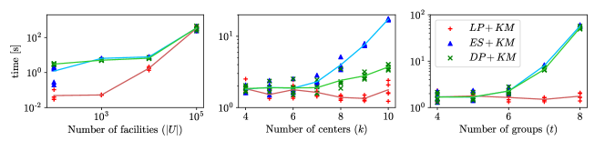
Figure 2. Scalability of bicriteria algorithm for $\text{\sc Div-}k\text{\sc-Means}$.

A.2. Proof of Lemma 5.6

In fact, we prove Theorem 4.1. We primarily focus on $\text{\sc Div-}k\text{\sc-Med}$, indicating the parts of the proof for $\text{\sc Div-}k\text{\sc-Means}$. In essence, to achieve the results for $\text{\sc Div-}k\text{\sc-Means}$, we need to consider squared distances which results in the claimed approximation ratio with same runtime bounds.

As mentioned before, to get a better approximation factor, the idea is to reduce the problem of finding an optimal solution to $k\text{\sc-Med-}k\text{\sc-PM}$ to the problem of maximizing a monotone submodular function. To this end, for each $S\subseteq\pazocal{F}$, we define the submodular function $\text{\sf improv}(S)$ that, in a way, captures the cost of selecting $S$ as our solution. To define the function improv, we add a fictitious facility $F^{\prime}_{i}$, for each $i\in[k]$ such that $F^{\prime}_{i}$ is at a distance $2\lambda^{*}_{i}$ for each facility in $\Pi_{i}$. We, then, use the triangle inequality to compute the distance of $F^{\prime}_{i}$ to all other nodes. Then, using an $(1-1/e)$-approximation algorithm (Line 12), we approximate improv. Finally, we return the set that has the minimum $k\text{\sc{-Median}}$ cost over all iterations.

Input: $J$, an instance of the $k\text{\sc-Med-}k\text{\sc-PM}$ problem

 $\epsilon^{\prime}$, a real number

1

Output: $S^{*}$, a subset of facilities

2

3$S^{*}\leftarrow\emptyset$, $\eta\leftarrow e\epsilon^{\prime}/2$

4 foreach ordered multiset $\{c^{\prime}_{i_{1}},\cdots,c^{\prime}_{i_{k}}\}\subseteq C^{\prime}$ of size $k$ do

5       foreach ordered multiset $\Lambda=\{\lambda_{i_{1}},\cdots,\lambda_{i_{k}}\}$ such that $\lambda_{i_{1}}\subseteq[[\Delta]_{\eta}]$ do

6             for $j=1$ to $k$ do

7                   $\Pi_{j}\leftarrow\{f\in E^{\prime}_{j}\mid d_{D}(f,c^{\prime}_{i_{j}})=\lambda_{i_{j}}\}$

8                   Add a fictitious facility $F^{\prime}_{j}$

9                   for $f\in\Pi_{j}$ do

10                         $d(F^{\prime}_{j},f)\leftarrow 2\lambda_{i_{j}}$

11                  for $f\notin\Pi_{j}$ do

12                         $d(F^{\prime}_{j},v)\leftarrow 2\lambda_{i_{j}}+\min_{f\in\Pi_{j}}d(f,v)$

13                  

14            for $S\subseteq F$, define $\textsf{improve}(S):=\textsf{cost}(C^{\prime},F^{\prime})-\textsf{cost}(C^{\prime},F^{\prime}\cup S)$ do

15                   $S_{max}\leftarrow S\subseteq\pazocal{F}$ that maximizes $\textsf{improve}(S)$ s.t. $|S\cap\Pi_{j}|=1,\forall j\in[k]$

16                   if $\textsf{cost}(C^{\prime},S_{max})<\textsf{cost}(C^{\prime},S^{*})$ then

17                         $S^{*}\leftarrow S$

18                  

19            

20      

return $S^{*}$

Algorithm 2 ${k\text{\sc-Med-}k\text{\sc-PM}(J=((U,d),\{E_{1},\cdots,E_{k}\},C^{\prime}),\epsilon^{\prime})}$

Correctness: Given $I=((U,d),F,C,\mathscr{G},\vec{r},k)$ . Let $\mathscr{J}:=\{J_{\ell}\}$ be the instances of $k\text{\sc-Med-}k\text{\sc-PM}$ generated by Algorithm 1 at Line 9 (For simplicity, we do not consider client coreset $C^{\prime}$ here). For correctness, we show that $F^{*}=\{f^{*}_{i}\}_{i\in[k]}\subseteq\pazocal{F}$ is feasible to $I$ if and only if there exists $J_{\ell^{*}}=((V,d),\{E^{*}_{1},\cdots,E^{*}_{k}\},C)\in\mathscr{J}$ such that $F^{*}$ is feasible to $J_{\ell^{*}}$. This is sufficient, since the objective function of both the problems is same, and hence returning minimum over $\mathscr{J}$ of an optimal (approximate) solution obtains an optimal (approximate resp.) solution to $I$. We need the following proposition for the proof.

Proposition A.1.

For all $E\in\mathscr{E}$, and for all $f\in E$, we have $\vec{\chi}_{f}=\vec{\chi}_{E}$.

Proof.

Fix $E\in\mathscr{E}$ and $f\in E$. Since $E\in\mathscr{E}$, there exists $\vec{\gamma}\in\{0,1\}^{t}$ such that $E_{\vec{\gamma}}=E$. But this means $\vec{\chi}_{E}=\vec{\gamma}$. On the other hand, since $f\in E_{\vec{\gamma}}$, we have that $\vec{\chi}_{f}=\vec{\gamma}$. ∎

Suppose $F^{*}=\{f^{*}_{i}\}_{i\in[k]}\subseteq\pazocal{F}$ is a feasible solution to $I:$ $\sum_{i\in[k]}\vec{\chi}_{f^{*}_{i}}\geq\vec{r}.$ Then, consider the instance $J_{\ell^{*}}=((V,d),\{E^{*}_{1},\cdots,E^{*}_{k}\},C)$ with $E^{*}_{i}=E_{\vec{\chi}_{f^{*}_{i}}}$, for all $i\in[k]$. Since,

$$\sum_{i\in[k]}\vec{\chi}_{E^{*}_{i}}=\sum_{i\in[k]}\vec{\chi}_{f^{*}_{i}}\geq\vec{r}$$

we have that $J_{\ell^{*}}\in\mathscr{J}$. Further, $F^{*}$ is feasible to $J_{\ell^{*}}$ since $F^{*}\cap E^{*}_{i}=f^{*}_{i}$ for all $i\in[k]$. For the other direction, fix an instance $J_{\ell^{*}}=((V,d),\{E^{*}_{1},\cdots,E^{*}_{k}\},C)\in\mathscr{J}$ and a feasible solution $F^{*}=\{f^{*}_{i}\}_{i\in[k]}$ for $J_{\ell^{*}}$. From Claim A.1 and the feasiblity of $F^{*}$, we have $\vec{\chi}_{f^{*}_{i}}=\vec{\chi}_{E^{*}_{i}}$. Hence,

$$\sum_{i\in[k]}\vec{\chi}_{f^{*}_{i}}=\sum_{i\in[k]}\vec{\chi}_{E^{*}_{i}}\geq\vec{r}$$

which implies $F^{*}=\{f^{*}_{i}\}_{i\in[k]}$ is a feasible solution to $I$. To complete the proof, we need to show that the distance function defined in Line 10 is a metric, and improv function defined in Line 11 is a monotone submodular function. Both these proofs are the same as that in (Cohen-Addad et al., 2019).

Approximation Factor: For $I=((U,d),F,C,\mathscr{G},\vec{r},k)$, let $I^{\prime}=((U,d),C^{\prime},F,\mathscr{G},\vec{r},k)$ be the instance with client coreset $C^{\prime}$. Let $F^{*}\subseteq\pazocal{F}$ be an optimal solution to $I$, and let $\tilde{F}^{*}\subseteq\pazocal{F}$ be an optimal solution to $I^{\prime}$. Then, from core-set Lemma 5.2, we have that

$$(1-\nu)\cdot\textsf{cost}(F^{*},C)\leq\textsf{cost}(F^{*},C^{\prime})\leq(1+\nu)\cdot\textsf{cost}(F^{*},C).$$

The following proposition, whose proof closely follows that in (Cohen-Addad et al., 2019), bounds the approximation factor of Algorithm 1.

Proposition A.2.

For $\epsilon^{\prime}>0$, let $J_{\ell}=((V,d),\{E_{1},\cdots,E_{k}\},C^{\prime},\epsilon^{\prime})$ be an input to Algorithm 2, and let $S^{*}_{\ell}$ be the set returned. Then,

$$\textsf{cost}(C^{\prime},S^{*}_{\ell})\leq(1+2/e+\epsilon^{\prime})\cdot\textsf{OPT}(J_{\ell}),$$

where $\textsf{OPT}(J_{\ell})$ is the optimal cost of $k\text{\sc-Med-}k\text{\sc-PM}$ on $J_{\ell}$. Similarly, for $\text{\sc Div-}k\text{\sc-Means}$,

$$\textsf{cost}(C^{\prime},S^{*}_{\ell})\leq(1+8/e+\epsilon^{\prime})\cdot\textsf{OPT}(J_{\ell}),$$

This allows us to bound the approximation factor of Algorithm 1.

$$\textsf{cost}(T^{*},C^{\prime})=\min_{J_{\ell}\in\mathscr{J}}\textsf{cost}(S^{*}_{\ell},C^{\prime})\leq(1+2/e+\epsilon^{\prime})\cdot\textsf{cost}(\tilde{F}^{*},C^{\prime})$$

$$\leq(1+2/e+\epsilon^{\prime})\cdot\textsf{cost}(F^{*},C^{\prime})\leq(1+2/e+\epsilon^{\prime})(1+\nu)\cdot\textsf{cost}(F^{*},C).$$

On the other hand, we have $\textsf{cost}(T^{*},C)\leq(1+2\nu)\cdot\textsf{cost}(T^{*},C^{\prime})$. Hence, using $\epsilon^{\prime}=\epsilon/4$ and $\nu=\epsilon/16$, we have

$$\textsf{cost}(T^{*},C) \leq(1+2/e+\epsilon^{\prime})(1+\nu)(1+2\nu)\cdot\textsf{cost}(F^{*},C)$$

$$\leq(1+2/e+\epsilon)\cdot\textsf{cost}(F^{*},C)$$

for $\epsilon\leq 1/2$. Analogous calculations holds for $\text{\sc Div-}k\text{\sc-Means}$. This finishes the proof of Lemma 5.6. Now, we prove Proposition A.2.

Proof.

Let $F^{*}_{\ell}$ be an optimal solution to $J_{\ell}$. Then, since $\textsf{cost}(C^{\prime},F^{\prime}\cup F^{*}_{\ell})=\textsf{cost}(C^{\prime},F^{*}_{\ell})$, we have that $F^{*}_{\ell}$ is a maximizer of the function $\text{\sf improv}(\cdot)$, defined at Line 11. Hence due to submodular optimization, we have that

$$\text{\sf improv}(S^{*}_{\ell})\geq(1-1/e)\cdot\text{\sf improv}(F^{*}_{\ell}).$$

Thus,

$$\text{\sf cost}(C^{\prime},S^{*}_{\ell}) =\text{\sf cost}(C^{\prime},F^{\prime}\cup S^{*}_{\ell})$$

$$=\text{\sf cost}(C^{\prime},F^{\prime})-\text{\sf improv}(S^{*}_{\ell})$$

$$\leq\text{\sf cost}(C^{\prime},F^{\prime})-(1-1/e)\cdot\text{\sf improv}(F^{*}_{\ell})$$

$$=\text{\sf cost}(C^{\prime},F^{\prime})-(1-1/e)\cdot\left(\text{\sf cost}(C^{\prime},F^{\prime})-\text{\sf cost}(C^{\prime},F^{*}_{\ell})\right)$$

$$=1/e\cdot\text{\sf cost}(C^{\prime},F^{\prime})+(1-1/e)\cdot\text{\sf cost}(C^{\prime},F^{*}_{\ell})$$

∎

The following proposition bounds $\text{\sf cost}(C^{\prime},F^{\prime})$ in terms of $\text{\sf cost}(C^{\prime},F^{*}_{\ell})$.

Proposition A.3.

$\text{\sf cost}(C^{\prime},F^{\prime})\leq(3+2\eta)\cdot\text{\sf cost}(C^{\prime},F^{*}_{\ell})$.

Setting $\eta=\frac{e}{2}\epsilon^{\prime}$, finishes the proof for $\text{\sc Div-}k\text{\sc-Med}$,

$$\text{\sf cost}(C^{\prime},S^{*}_{\ell}) \leq(3+e\epsilon^{\prime})/e\cdot\text{\sf cost}(C^{\prime},F^{*}_{\ell})+(1-1/e)\cdot\text{\sf cost}(C^{\prime},F^{*}_{\ell})$$

$$\leq(1+2/e+\epsilon^{\prime})\cdot\text{\sf cost}(C^{\prime},F^{*}_{\ell}).$$

For $\text{\sc Div-}k\text{\sc-Means}$, setting $\eta=\frac{e}{16}\epsilon^{\prime}$, finishes the proof of Proposition A.2,

$$\text{\sf cost}(C^{\prime},S^{*}_{\ell}) \leq(3+2e\epsilon^{\prime}/16)^{2}/e\cdot\text{\sf cost}(C^{\prime},F^{*}_{\ell})+(1-1/e)\text{\sf cost}(C^{\prime},F^{*}_{\ell})$$

$$\leq(1+8/e+\epsilon^{\prime})\cdot\text{\sf cost}(C^{\prime},F^{*}_{\ell}).$$

for $\eta\leq 1$.

Proof.

To this end, it is sufficient to prove that for any client $c^{\prime}\in C^{\prime}$, it holds that $d(c^{\prime},F^{\prime})\leq(3+2\eta)d(c^{\prime},F^{*}_{\ell})$. Fix $c^{\prime}\in C$, and let $f^{*}_{\ell_{j}}\in F^{*}_{\ell}$ be the closest facility in $F^{*}_{\ell}$ with $\lambda^{*}_{j}$ such that $\lambda^{*}_{j}=d(c^{\prime}_{i_{j}},f^{*}_{\ell_{j}})$. Now,

$$d(c^{\prime},f^{*}_{\ell_{j}})\geq d(c^{\prime}_{i_{j}},f^{*}_{\ell_{j}})\geq(1+\eta)^{([\lambda^{*}_{j}]_{D}-1)}\geq\frac{\lambda^{*}_{j}}{1+\eta}.$$

Using, triangle inequality and the above equation, we have,

$$d(c^{\prime},F^{\prime}) \leq d(c,F^{\prime}_{j})\leq d(c^{\prime},F^{*}_{\ell_{j}})+d(F^{*}_{\ell},F^{\prime})\leq d(c^{\prime},f^{*}_{\ell_{j}})+2\lambda^{*}_{j}$$

$$\leq(3+2\eta)d(c^{\prime},f^{*}_{\ell_{j}}).$$

∎

A.3. Other proofs

Proof of Corollary 3.1

SETH implies that there is no $\mathscr{O}(|V|^{k-\epsilon})$ algorithm for $k\text{\sc-Dom\-Set}$, for any $\epsilon>0$. The reduction in (Thejaswi et al., 2021b, Lemma 1) creates an instance of $\text{\sc Div-}k\text{\sc-Med}$ ($\text{\sc Div-}k\text{\sc-Means}$ resp.) where $F=V$. Hence, any FPT exact or approximate algorithm running in time $\mathscr{O}(|F|^{k-\epsilon})$ for $\text{\sc Div-}k\text{\sc-Med}$ ($\text{\sc Div-}k\text{\sc-Means}$ resp.) contradicts SETH.

$\hfill\square$

Proof of Proposition 3.2

First, note that any FPT algorithm $\mathscr{A}$ achieving a multiplicative factor approximation for $\text{\sc Div-}k\text{\sc-Med}$ ($\text{\sc Div-}k\text{\sc-Means}$ resp.) needs to solve the lower bound requirements first. Since these requirements capture $k\text{\sc-Dom\-Set}$ (Thejaswi et al., 2021b, Lemma 1), it means $\mathscr{A}$ solves $k\text{\sc-Dom\-Set}$ in FPT time, which is a contradiction. Finally, noting the fact that finding even $f(k)$ size dominating set, for any $f(k)$, is also $\mathbf{W[1]}$-hard due to (S. et al., 2019) finishes the proof.

$\hfill\square$

References

- (1)
- Ahmadian et al. (2019) Sara Ahmadian, Ashkan Norouzi-Fard, Ola Svensson, and Justin Ward. 2019. Better guarantees for k-means and euclidean k-median by primal-dual algorithms. SIAM J. Comput. 49, 4 (2019), FOCS17–97.
- Anuthors (2022) Anonymous Anuthors. 2022. Clustering with fair center representation: experimental v1.0. https://github.com/nla2ifyhalispd/div-k-median.
- Arya et al. (2001) Vijay Arya, Naveen Garg, Rohit Khandekar, Adam Meyerson, Kamesh Munagala, and Vinayaka Pandit. 2001. Local-Search Heuristics for -Median and Facility-Location Problems. In STOC.
- Arya et al. (2004) Vijay Arya, Naveen Garg, Rohit Khandekar, Adam Meyerson, Kamesh Munagala, and Vinayaka Pandit. 2004. Local search heuristics for -median and facility location problems. SIAM Journal on computing 33, 3 (2004), 544–562.
- Bachem et al. (2017) Olivier Bachem, Mario Lucic, and Andreas Krause. 2017. Practical coreset constructions for machine learning. arXiv preprint arXiv:1703.06476 (2017).
- Backurs et al. (2019) Arturs Backurs, Piotr Indyk, Krzysztof Onak, Baruch Schieber, Ali Vakilian, and Tal Wagner. 2019. Scalable fair clustering. In ICML.
- Bercea et al. (2019) Ioana O Bercea, Martin Groß, Samir Khuller, Aounon Kumar, Clemens Rösner, Daniel R Schmidt, and Melanie Schmidt. 2019. On the Cost of Essentially Fair Clusterings. In APPROX.
- Berk et al. (2021) Richard Berk, Hoda Heidari, Shahin Jabbari, Michael Kearns, and Aaron Roth. 2021. Fairness in criminal justice risk assessments: The state of the art. Sociological Methods & Research 50, 1 (2021), 3–44.
- Biddle (2020) Justin B Biddle. 2020. On predicting recidivism: Epistemic risk, tradeoffs, and values in machine learning. Canadian Journal of Philosophy (2020), 1–21.
- Byrka et al. (2014) Jarosław Byrka, Thomas Pensyl, Bartosz Rybicki, Aravind Srinivasan, and Khoa Trinh. 2014. An improved approximation for k-median, and positive correlation in budgeted optimization. In SODA. SIAM, 737–756.
- Calinescu et al. (2011) Gruia Calinescu, Chandra Chekuri, Martin Pal, and Jan Vondrák. 2011. Maximizing a monotone submodular function subject to a matroid constraint. SIAM J. Comput. 40, 6 (2011), 1740–1766.
- Charikar et al. (2002) Moses Charikar, Sudipto Guha, Éva Tardos, and David B. Shmoys. 2002. A Constant-Factor Approximation Algorithm for the k-Median Problem. JCSS 65, 1 (2002), 129–149.
- Chierichetti et al. (2017) Flavio Chierichetti, Ravi Kumar, Silvio Lattanzi, and Sergei Vassilvitskii. 2017. Fair clustering through fairlets. In NeurIPS.
- Cohen-Addad et al. (2019) Vincent Cohen-Addad, Anupam Gupta, Amit Kumar, Euiwoong Lee, and Jason Li. 2019. Tight FPT Approximations for k-Median and k-Means. In ICALP, Vol. 132. Dagstuhl, Dagstuhl, Germany, 42:1–42:14.
- Cygan et al. (2016) Marek Cygan, Holger Dell, Daniel Lokshtanov, Dániel Marx, Jesper Nederlof, Yoshio Okamoto, Ramamohan Paturi, Saket Saurabh, and Magnus Wahlström. 2016. On Problems as Hard as CNF-SAT. ACM Trans. on Algorithms 12, 3 (2016).
- Cygan et al. (2015) Marek Cygan, Fedor V Fomin, Łukasz Kowalik, Daniel Lokshtanov, Dániel Marx, Marcin Pilipczuk, Michał Pilipczuk, and Saket Saurabh. 2015. Parameterized algorithms. Vol. 4. Springer.
- Dua and Graff (2017) Dheeru Dua and Casey Graff. 2017. UCI Machine Learning Repository. http://archive.ics.uci.edu/ml
- Dwork et al. (2018) Cynthia Dwork, Nicole Immorlica, Adam Tauman Kalai, and Max Leiserson. 2018. Decoupled classifiers for group-fair and efficient machine learning. In Conference on fairness, accountability and transparency. PMLR, 119–133.
- Feldman and Langberg (2011) Dan Feldman and Michael Langberg. 2011. A Unified Framework for Approximating and Clustering Data. In STOC. ACM, 569–578.
- Fu et al. (2020) Zuohui Fu, Yikun Xian, Ruoyuan Gao, Jieyu Zhao, Qiaoying Huang, Yingqiang Ge, Shuyuan Xu, Shijie Geng, Chirag Shah, Yongfeng Zhang, et al. 2020. Fairness-aware explainable recommendation over knowledge graphs. In SIGIR.
- Guha and Khuller (1998) Sudipto Guha and Samir Khuller. 1998. Greedy Strikes Back: Improved Facility Location Algorithms. In SODA. SIAM, USA, 649–657.
- Hajiaghayi et al. (2010) MohammadTaghi Hajiaghayi, Rohit Khandekar, and Guy Kortsarz. 2010. Budgeted Red-Blue Median and Its Generalizations. In ESA.
- Hajiaghayi et al. (2012) M Hajiaghayi, Rohit Khandekar, and Guy Kortsarz. 2012. Local-search algorithms for the red-blue median problem. Algorithmica 63, 4 (2012), 795–814.
- Hardt et al. (2016) Moritz Hardt, Eric Price, and Nati Srebro. 2016. Equality of opportunity in supervised learning. In NeurIPS.
- Huang et al. (2019) Lingxiao Huang, Shaofeng Jiang, and Nisheeth Vishnoi. 2019. Coresets for clustering with fairness constraints. In NeurIPS.
- Impagliazzo and Paturi (2001) Russell Impagliazzo and Ramamohan Paturi. 2001. On the Complexity of -SAT. JCSS 62, 2 (2001), 367–375.
- Kanungo et al. (2004) Tapas Kanungo, David M Mount, Nathan S Netanyahu, Christine D Piatko, Ruth Silverman, and Angela Y Wu. 2004. A local search approximation algorithm for k-means clustering. Computational Geometry 28, 2-3 (2004), 89–112.
- Krishnaswamy et al. (2011) Ravishankar Krishnaswamy, Amit Kumar, Viswanath Nagarajan, Yogish Sabharwal, and Barna Saha. 2011. The matroid median problem. In SODA.
- Raghavan and Tompson (1987) Prabhakar Raghavan and Clark D. Tompson. 1987. Randomized Rounding: A Technique for Provably Good Algorithms and Algorithmic Proofs. Combinatorica 7, 4 (dec 1987), 365–374. https://doi.org/10.1007/BF02579324
- Rösner and Schmidt (2018) Clemens Rösner and Melanie Schmidt. 2018. Privacy Preserving Clustering with Constraints. In ICALP.
- S. et al. (2019) Karthik C. S., Bundit Laekhanukit, and Pasin Manurangsi. 2019. On the Parameterized Complexity of Approximating Dominating Set. Journal of ACM 66, 5 (2019), 38 pages.
- Schmidt et al. (2019) Melanie Schmidt, Chris Schwiegelshohn, and Christian Sohler. 2019. Fair Coresets and Streaming Algorithms for Fair -means. In WAOA.
- Thejaswi et al. (2021a) Suhas Thejaswi, Bruno Ordozgoiti, and Aristides Gionis. 2021a. Diversity-aware -median : Clustering with fair center representation. arXiv:2106.11696 [cs.DS]
- Thejaswi et al. (2021b) Suhas Thejaswi, Bruno Ordozgoiti, and Aristides Gionis. 2021b. Diversity-aware -median: Clustering with fair center representation. In ECML-PKDD. Springer, 1–16.
- Vassilvitskii and Arthur (2006) Sergei Vassilvitskii and David Arthur. 2006. k-means++: The advantages of careful seeding. In SODA. 1027–1035.
- Zafar et al. (2017) Muhammad Bilal Zafar, Isabel Valera, Manuel Gomez Rodriguez, and Krishna P Gummadi. 2017. Fairness beyond disparate treatment & disparate impact: Learning classification without disparate mistreatment. In WWW. 1171–1180.