On Approximate Sequencing Policies for Linear Storage Devices

Abstract

This paper investigates sequencing policies for file reading requests in linear storage devices, such as magnetic tapes. Tapes are the technology of choice for long-term storage in data centers due to their low cost and reliability. However, their physical structure imposes challenges to data retrieval operations reflected in classic optimization and operations research problems. In this work, we provide a theoretical and numerical performance analysis of low-complexity algorithms under deterministic, stochastic, and online settings, which are key in practice due to their interpretability and the large scale of existing data services. In the deterministic setting, we show that traditional policies, such as first-in first-out (FIFO), have arbitrarily poor performance, and we develop and investigate new constant-factor approximations. For the stochastic setting, we present a fully polynomial-time approximation scheme that weighs files based on their access frequencies. Finally, we investigate an online extension and propose a new algorithm with constant competitive-factor guarantees. Our numerical analysis on synthetic and real-world data suggest that the proposed algorithms may significantly outperform policies currently adopted in practice with respect to average reading times.

1 Introduction

Scheduling methodologies play a pivotal role in the operations of data storage solutions, an industry that is forecasted to reach a valuation of US $35 billion in 2022 (Yezhkova et al. 2020). Data storage solutions offer a portfolio of random-access technologies for quick and recurrent file access, such as non-volatile memories and solid-state drivers, as well as cold-storage technologies where data are preserved for less frequent but longer-term access. Due to the critical relevance of both technologies to data processing, the effective storage and retrieval of files have led to an extensive number of classical problems in the operations research and optimization literature (see, e.g., §A.4 in Garey and Johnson 1979, Parker and Ram 1997, and Schaeffer and Casanova 2011).

In this work, we investigate file retrieval policies for linear storage devices, or more precisely, magnetic tapes. Tapes are the standard choice in cold storage due to their compelling cost, space, and security advantages (Lantz 2018). For example, due to increase in cybersecurity threats and demand for high-volume storage, shipments for tape-based storage media increased by 40% in 2021 (Pires 2022). Tapes are extensively used by the entertainment industry (Coughlin 2019), oil companies (Gaul et al. 2007), space mission analysis (NASA 2021), and for multi-year research data for projects such as the Large Hadron Collider (Cavalli et al. 2010). Standards for magnetic tapes are open and established by the Linear Tape-Open (LTO) consortium (LTO 2021), composed of Hewlett Packard Enterprise, Quantum, and IBM, the latter a partner in this research study.

Figure 1: Example of tape movement when reading files $3$, $2$, and $1$, in this order. Reading operations start at the rightmost file. Solid (colored) and dashed (black) arcs depict repositioning and reading operations, respectively. Labels represent the distance traversed when the movement is finished.

The main characteristic of tapes is that files are distributed sequentially and contiguously throughout their tracks, leading to difficult operational aspects that share a close relationship with fundamental single-resource scheduling problems (Pinedo 2016). Figure 1 illustrates a tape structure with three files with sizes $15$, $4$, and $2$ bits. Files have a left-to-right orientation, in that a retrieval operation must read the files linearly from their leftmost bit to their rightmost bit. Restrictions on the tape head also specify that only one file can be processed at a time. Thus, when reading a file, the tape head must first reposition itself to the left of the file, read it by traversing its bits, and again reposition itself to the left of the next file in the reading sequence. The figure depicts the retrieval sequence (3, 2, 1) and the total distance traversed for each repositioning and reading operation, assuming that the tape starts at the end of the rightmost file.

Our work investigates the retrieval problem faced by data centers considering offline and online settings. Specifically, in each planning period the data center receives a service request from customers or automated systems describing a set of files to be recovered from a tape. The objective is to define a sequence of file reads to minimize the total (or average) response time, i.e., the time elapsed until each file starts to be read for the first time. This is a standard measure, as it captures quality of service and technical considerations (Hillyer and Silberschatz 1996b). For instance, in Figure 1 the response time is $2+10+33=45$ for a tape speed of one time unit per bit.

The challenge in practical storage systems is scalability and interpretability. The deterministic problem variant (i.e., the files to retrieve are known in advance) is tractable with a time complexity that is $\mathcal{O}(n^{4})$ in the number of files $n$. However, tapes often include thousands of files, and in standard guidelines no more than a few seconds is alloted to file-sequencing algorithms; for example, to enable batch analytics directly on archived data (Kathpal and Yasa 2014). Tape hardware is also limited to less expensive, slower processors that are more energy efficient given the scale of operations. Further, data centers have a strong preference for low-complexity and understandable algorithms that can be justified, as small policy changes have a propagating effect in file retrieval times due to the large number of tapes and files in a data center. Not surprisingly, the standard tape file system employs first-in first-out (FIFO) heuristic strategies (ISO/IEC-20919:2016 2016), processing files in the order that they are received.

In view of these properties, this work provides a formal study of efficient but interpretable sequencing policies considering deterministic, stochastic, and online service request variants. In the deterministic setting, we consider a cold-storage environment where batches of read requests are uncorrelated but possibly few and far between; thus, the reading sequence can be processed offline. We investigate the theoretical performance of FIFO and approximation algorithms based on intuitive reverse- and forward-reading directions. We also show that this perspective reveals an alternative polynomial-time exact approach based on dynamic programming (DP).

The stochastic setting assumes that service requests are frequent and that a probability distribution over file requests is known. Our objective is to leverage distributional information to predetermine a reading sequence to be applied to all requests, which is in line with the previous interpretable policies. We show that, in this setting, the proposed DP for the exact deterministic approach can be adapted to a fully polynomial-time approximation scheme for the stochastic problem. Of particular importance is that the underlying DP only needs to be solved once, and the resulting sequence can be reapplied if the distributions remain unchanged.

Finally, we investigate an online setting incorporating real-time service requests when no distribution information is available. We first show that FIFO has an arbitrarily poor performance in worst-case but common scenarios. We then develop a constant-factor competitive policy by iteratively alternating linear forward and backward reading operations. We also show that no competitive factor exists for an alternative objective criterion that considers file release times.

To evaluate the policies, we provide a numerical study using artificial and real tape systems, the latter used for satellite imaging managed by an industry partner. The results suggest that the ordering of policies with respect to their theoretical performance is also observed empirically. In particular, our best proposed algorithm with constant-factor guarantee is often optimal and of sufficiently low complexity to be adopted in practice. Moreover, if distributional information is available, the sequence derived from the approximation scheme outperforms approximate policies, especially if the request probabilities are relatively high.

Summary of contributions. The primary contribution of this work is the formal study of approximate but low-complexity and interpretable policies for sequencing tasks in a linear storage device, considering both deterministic and uncertain cases. This adds to the existing literature that has focused on offline heuristics (Zhang et al. 2006, Schaeffer and Casanova 2011). In the deterministic setting, we identify worst-case performance ratios as well as cases where the approximations are optimal. In the stochastic setting, we adapt a polynomial-time dynamic program to develop a fully polynomial approximation scheme for use when access frequencies are available. For the online case, we develop constant-factor approximations and inapproximability of certain objective criteria. Finally, we analyze the numerical performance of the policies and draw insights on their empirical approximation ratio based on the instance structure, such as tape size and file size variance.

Paper structure. The paper is organized as follows. §2 reviews existing work and discusses the relationship between linear tape storage and existing scheduling problems. §3 formalizes the problem, and §4 investigates the deterministic setting. §5 studies the stochastic setting and introduces the fully polynomial time approximation scheme. §6 discusses the online approach and associated competitive ratios. §7 presents our numerical study. Finally, §8 concludes and discusses future work. Proofs omitted in the main text are included in the electronic appendix.

2 Related Work

Scheduling for sequential storage systems is a classical research stream in both the operations and computer science literature. To the best of our knowledge, Day (1965) is the first to formalize a request problem over a multiple-file data storage system, proposing an integer programming (IP) formulation and heuristics considering potentially overlapping files. We note that model-based approaches such as IP typically do not scale due to the strict solution time adopted in industry and the limited processing power of tape hardware.

Early work has primarily focused on storage design, i.e., how to arrange files in a storage medium to minimize the long-run average response time. The study by Cody and Coffman Jr (1976) was pioneering in this field, demonstrating that assigning files of the same size to different storage sectors is NP-hard if the file access distribution is known; other related problems are presented in Section A.4 of Garey and Johnson (1979).

The simplest variant with no uncertainty or side constraint in tape design is the so-called optimal storage in tapes, which can be efficiently solved by a greedy algorithm that sorts file in ascending size order (Parker and Ram 1997). It has since become a seminal example of greedy algorithms and fostered related fields, such as greedoid theory (Korte et al. 2012). In this paper, we focus on the operational aspect of establishing file read orderings, assuming that (i) files have already been placed on the tape and (ii) access distributions may change. Further, we show that greedy approaches are suboptimal and investigate their theoretical performance ratios.

Recent literature has focused on heuristic policies for tapes with varying organizational structures. Most notably, Hillyer and Silberschatz (1996a) and Sandstå and Midtstraum (1999) investigated the problem of estimating tape velocity in serpentine tapes, proposing simple scheduling heuristics that orders files based on their physical position in the tape. Hillyer and Silberschatz (1996b) developed a greedy heuristic based on an assymetric traveling salesperson problem (TSP) reduction for tertiary storage systems, simulating its performance against a pre-defined weave ordering for a serpentine tape. Similar sorting or greedy heuristics are found in other file systems, e.g., as discussed in Zhang et al. (2006) and Schaeffer and Casanova (2011).

Our problem is closely related to the traveling repairman problem (TRP) (Fischetti et al. 1993, Coene et al. 2011, Pinedo 2016). Particularly relevant to our work is the line-TRP, where vertices are distributed on a straight line. While the TRP is NP-complete in general (Afrati et al. 1986, Simchi-Levi and Berman 1991), the line-TRP can be solved in polynomial time if the processing times are zero (Bock 2015, Psaraftis et al. 1990). The complexity of the line-TRP with general processing times is still unknown. A related problem is the dial-a-ride on the line (line-DR), which transports products between pairs of vertices using one or more capacitated vehicles. de Paepe et al. (2004) present a classification of dial-a-ride problems, noting that minimizing the total completion times for the line-DR is NP-hard even if vehicles have capacity one. We discuss the formal relationship between our problem and the TRP in §3.2.

Online variations of the problems above are also related to sequential storage problems. One example is the online TSP on the line, in which new vertices to visit appear during a tour (Jaillet and Wagner 2006). Bjelde et al. (2017) present a 1.64-competitive algorithm for the online TSP on the line, which is the best-possible competitive factor for the problem (Ausiello et al. 2001).

For linear storage systems, Honoré et al. (2022) showed that the deterministic problem is solvable with time complexity that is quartic in the number of files on the tape, a result which we also obtain independently from an alternative perspective. Moreover, in a preliminary version of this work, Cardonha and Real (2016) proposed heuristic strategies to minimize flow time for interleaved read and write operations. In contrast to this earlier work, we consider the more realistic cold-storage setting where the tape is locked (no writes are possible), incorporate the response-time criteria, and provide a study of the theoretical worst-case performance of approximate methodologies for deterministic and uncertain variants of the problem.

3 The Linear Tape Sequencing Problem

In this section, we formalize in §3.1 the base linear tape sequencing model to be investigated in this work. Next, in §3.2 we describe its connection to two classical problems in the scheduling and routing literature. Finally, in §3.3 we discuss the practical assumptions underlying the model.

3.1 Problem Description

A tape is a set of $n$ files $\mathscr{F}\equiv\{1,\dots,n\}$ distributed sequentially and contiguously on a line discretized by bit units. The files have a left-to-right storage orientation, i.e., each file $i\in\mathscr{F}$ begins in its left-bit position $\ell_{i}$ and has a size of $s_{i}$ bits. The right-bit position of file $i$ is the first bit where the succeeding file starts, i.e., $r_{i}=\ell_{i}+s_{i}$. The first file begins at the initial position of the tape, $\ell_{1}=0$, and the last file ends at position $L=r_{n}$, which coincides with the logical end of the tape. The tape length is defined by $L=\sum\limits_{i\in\mathscr{F}}s_{i}$.

The tape is traversed by its head driver, which always start at the end of the tape at bit $L$. At each decision epoch, the data center receives a subset of files in $\mathscr{F}$ to be retrieved from the tape. We introduce a parameter $w_{i}=1$ to indicate if file $i\in\mathscr{F}$ is requested, and $w_{i}=0$ otherwise. We assume that the first file is always requested, $w_{1}=1$; otherwise, the left-position of the tape can be adjusted accordingly. The objective is to find a permutation $\boldsymbol{\pi}=(\pi_{1},\dots,\pi_{n})$ of $\mathscr{F}$ that minimizes the total response time of requested files in the reading sequence implied by $\boldsymbol{\pi}$. More precisely, the response time of the $t$-th file, $\pi_{t}\in\mathscr{F}$, is the time elapsed until the first bit of $\pi_{t}$ is reached, i.e.,

$$R_{t}(\boldsymbol{\pi})\equiv\sum_{t^{\prime}=1}^{t}\left(s_{\pi_{t^{\prime}-1}}+d_{\pi_{t^{\prime}-1},\pi_{t^{\prime}}}\right)\nu,$$ (1)

where $s_{\pi_{0}}=0$, $r_{\pi_{0}}$ is the position at which the tape head begins, $d_{\pi_{t^{\prime}-1},\pi_{t^{\prime}}}\equiv|\ell_{j}-r_{i}|$ accounts for the time spent reading $\pi_{t^{\prime}-1}$ and repositioning the right-bit position of $\pi_{t^{\prime}-1}$ to the left-bit position of $\pi_{t^{\prime}}$, and $\nu$ is the velocity of the tape in time units per bit. We assume without loss of generality that $\nu=1$. Thus, the deterministic linear tape sequencing problem (LTS) solves

$$R^{*}\equiv\min_{\boldsymbol{\pi}}\sum_{t=1}^{n}w_{\pi_{t}}R_{t}(\boldsymbol{\pi}).$$ (LTS)

Note that $n=3$, $s_{1}=r_{1}=\ell_{2}=15$, and $r_{3}=L=15+4+2=21$ for the example in Figure 1. For an additional illustration, we also include a larger example in A of the electronic companion comparing the response time of two different sequences.

3.2 Connection to Scheduling and Routing

The LTS shares connections with other fundamental optimization models from the scheduling and routing literature. In particular, note that, for $t>1$, we have $R_{t}(\boldsymbol{\pi})=R_{t-1}(\boldsymbol{\pi})+\left(s_{\pi_{t-1}}+d_{\pi_{t-1},\pi_{t}}\right)$ in (1). Expanding each term in the summation of the objective provides the reformulation

$$R^{*}=\min_{\boldsymbol{\pi}}\;\sum_{t=1}^{n}\left(m-\sum_{t^{\prime}=1}^{t-1}w_{\pi_{t^{\prime}}}\right)\left(s_{\pi_{t-1}}+d_{\pi_{t-1},\pi_{t}}\right),$$ (2)

where $m=\sum\limits_{i\in\mathscr{F}}w_{i}$ is the number of requested files. Thus, $R^{*}$ is equivalent to a latency (or time-dependent) cost function in scheduling. That is, prior to reading a file at the $t$-th position of the sequence, each bit the tape head traverses increases the total response time by the quantity $\left(m-\sum\limits_{t^{\prime}=1}^{t-1}w_{\pi_{t^{\prime}}}\right)$, depicting how many requests are left to be serviced. Based on this perspective, we show below that the LTS is a special case of the traveling repairperson problem (TRP) and the dial-a-ride problem. Thus, our results are applicable if the structure of the LTS is present.

Traveling Repairperson Problem (TRP). Given a set of points $\mathcal{V}\cup\{0\}$ and symmetric distances $D_{i,j}$ for any pair $i,j\in\mathcal{V}\cup\{0\}$, the TRP asks for a Hamiltonian tour starting at $0$ that minimizes the sum of distances traversed from point $0$ to each other point in the tour. We can cast the LTS as an asymmetric variant of the TRP as follows. The vertex $0$ is represented by an artificial zero-sized file $n+1$ located at the end of the tape, i.e., $\ell_{n+1}=r_{n+1}=L$, while the remaining points $\mathcal{V}=\{i\in\mathscr{F}\colon w_{i}=1\}$ are mapped to requested files. The distances between any $i,j\in\mathcal{V}$ are $D_{i,j}=s_{i}+d_{i,j}$ and $D_{j,i}=s_{j}+d_{j,i}$. That is, during a tour, we arrive on the left $\ell_{i}$ of a file $i$, and moving to the next file $j$ requires us to first traverse the length $s_{i}$ of $i$. Thus, the LTS is also a special case of the time-dependent TSP (Abeledo et al. 2013).

Dial-a-ride problem (DARP). Let $(o_{1},q_{1}),(o_{2},q_{2}),\dots,(o_{n},q_{n})$ be a set of pickup-and-delivery pairs, where each $o_{t}$ and $q_{t}$ is an origin point and a destination point, respectively. The DARP asks for vehicle routes to serve each pair while observing vehicle capacities and a quality metric associated with the distance traversed. The LTS corresponds to a DARP with a single vehicle of unitary capacity. That is, the requests are distributed on a line and each mapped to a requested file $i$, $w_{i}=1$, with $o_{t}=\ell_{i}$ and $q_{t}=r_{i}$. Moreover, $o_{t}\leq q_{t}$, i.e., the vehicle always moves from the left to the right when delivering a request, and all requests are positioned on the left of the start point of the vehicle. The objective is to minimize the distances to reach each origin point. In general, the line variant of DARP with a single vehicle and capacity one is NP-complete (de Paepe et al. 2004).

3.3 Practical Considerations

Next, we discuss the modeling assumptions and reasoning underlying the LTS. In our setting, all reading operations concern files located in the same data track, i.e., the tape only moves horizontally. While generally tapes may have other organizational structures, such as a serpentine arrangement, our single-track setting results in a linear positioning of the files, as is common and desirable by data center managers to preserve file locality (Oracle 2011). For reference, a single track of a modern tape (e.g., IBM TS1160) may store up to 400 GB of data.

Tape hardware consists of a single reader, so only one file is read at a time. To position the tape head at a particular bit location, the tape medium is either rewound or fast-forwarded accordingly, which we refer to as tape head positioning in this work. We also note that files are read from left to right. Such a reading (or traversal) direction is due to an operational restriction of tape hardware, as data cannot be retrieved when the track is traversed backwards (ISO/IEC-20919:2016 2016).

The tape heads start at the last position $L$ because of the append-base nature of tapes. That is, tapes always store their table of contents (TOC) with the list of files, their sizes, and corresponding positions at the last bit $L$ of the customer-provided data. When loading a tape, the driver must always read the TOC first to locate the remaining files, which positions the head at $L$.

We assume that the tape medium is rewound and fast-forwarded at a constant speed $\nu$. This is a standard modeling simplification in tape design and scheduling, as the physical components of a tape drive are mechanical and therefore require acceleration and deceleration. Finally, we note that the tape speed is not affected by its traversal direction or the execution of a reading operation.

4 The LTS with Deterministic Service Requests

This section investigates the offline LTS, where we establish $\pi$ knowing all files that have been requested. We begin in §4.1 by describing a partition of a solution into stages, which will serve as the basis of our results. We then analyze current policies in §4.2. Next, in §4.3 we propose two new constant-ratio policies that are also easy to justify and implement. Finally, in §4.4 we show a more technical result of a polynomial-time dynamic program based on the stage partioning constructs.

4.1 Stage Partitioning

The linear structure of tapes implies a partition of any sequence $\boldsymbol{\pi}$ in stages of directional movement. Specifically, note that the tape head will always move to bit 0 to read the first file. We state this in Definition 1, which is key for drawing policy intuition.

Definition 1 (Rewind and Forward Stages).

The rewind stage of $\boldsymbol{\pi}$ refers to the set of reading operations and translational movements prior to reaching bit 0 for the first time. The forward stage refers to all movements and reading operations after the rewind stage.

Given a sequence $\boldsymbol{\pi}$, we denote by $\mathcal{R}_{\boldsymbol{\pi}}$ and $\mathcal{F}_{\boldsymbol{\pi}}\equiv\mathscr{F}\setminus\mathcal{R}_{\boldsymbol{\pi}}$ the set of files read during the rewind and forward stages, respectively. In the example shown in Figure 1, $\mathcal{R}_{\boldsymbol{\pi}}=\{2,3\}$ and $\mathcal{F}_{\boldsymbol{\pi}}=\{1\}$; note that file 1 always belongs to the the forward stage. Proposition 1 shows that once the forward stage begins, the tape head only needs to perform a single left-to-right movement. Consequently, we can restrict our attention to cases where bit 0 is reached only once.

Proposition 1 (Forward-Stage Ordering).

There exists an optimal sequence $\boldsymbol{\pi}^{*}$ such that the forward-stage files are read in ascending order, i.e., $\pi^{*}_{t}<\pi^{*}_{t+1}$ for all $\pi^{*}_{t},\pi^{*}_{t+1}\in\mathcal{F}_{\boldsymbol{\pi}^{*}}$, $t<n$.

4.2 Analysis of Low-Complexity Policies

We now analyze three low-complexity policies that are adopted in practice. We first provide a general description and formalize their theoretical performance in Proposition 2.

First-In, First-Out (FIFO). The FIFO policy, featured in tape management software, sequences files according to the (typically arbitrary) order determined by the system that submitted the requests. FIFO is equivalent to a fully randomized policy and, thus, can deliver arbitrarily poor results.

First-File-First (FIFF). The FIFF policy reads files in ascending order of their indices, i.e., it generates a sequence $\boldsymbol{\pi}$ such that $\pi_{i}<\pi_{i+1}$ for all $i=1,\dots,n$. Thus, the policy delays all files to the forward stage. The practical intuition is that the response time would be low because the tape head makes only two movements, one to rewind the tape to its bit 0 and another to read the files in a single pass. Indeed, FIFF delivers strong constant-factor approximations in line routing problems (e.g., Bhattacharya et al. 2008).

Shortest Size First (SSF). The SSF reads files in ascending order of file size, i.e., it is a generalization of the classical shortest processing time first (SPT) policy and has time complexity of $\mathcal{O}(m\log m)$. The motivation follows from the latency-type objetive reformulation (2), where the SPT is optimal for related scheduling problems with similar criteria (Pinedo 2016). The SSF also solves the optimal storage in tapes problem (§2).

Proposition 2 (Performance of FIFO, FIFF, and SSF).

The following statements hold:

• FIFO, FIFF, and SSF are $\Omega(n)$-approximations for the LTS.

• FIFF is optimal if all the $n$ files in the tape are requested and they are of the same size.

Contrary to intuition, Proposition 2 shows that FIFF delivers arbitrarily poor solutions to the LTS, similar to FIFO. The worst-case scenario occurs in the presence of large requested files close to the end of the tape, as reading them penalizes requested files positioned in the beginning of the tape; SSF also has arbitrarily poor performance in these cases. Nonetheless, FIFF is optimal for a special scenario where all file sizes are equal. This is observed in practice for certain application domains, such as images or videos with the same resolutions or frame rates.

4.3 Constant-Ratio Approximation Policies

The policies presented in §4.2 are common in practice because they are scalable and simple to justify. However, their approximation ratios can be significantly high, which is also reflected in our empirical results (§7). Below, we introduce two alternative interpretable policies with stronger constant-factor theoretical guarantees and better empirical performance.

First-File-Last (FILA). The FILA policy is the reverse of FIFF, in that it services all requested files, except the first, in the rewind stage. That is, it generates a sequence $\boldsymbol{\pi}$ in constant time such that the contiguous subsequence $(\pi_{1},\pi_{2},\dots,\pi_{m-1},\pi_{m})$ that prefixes $\boldsymbol{\pi}$ spans the $m$ requested files and $\pi_{1}>\pi_{2}>\dots>\pi_{m}=1$. In other words, requested files are read in descending order.

FILA is akin to a myopic policy because files closest to the tape head are read first. We show in Proposition 3 that it is a 3-approximation. Further, FILA is also optimal for the case where all files in the tape have equal size, but it does not require all tape files to be requested as in FIFF.

Proposition 3 (FILA Performance).

The FILA policy is a 3-approximation algorithm for the LTS. Moreover, it is optimal if all tape files are of the same size.

Large-Files-Last Policy (LFL). The worst-case scenario of FILA occurs if some files with requests are considerably larger than others, especially if they are located at the end of the tape. Servicing such large files in the rewind stage delays all subsequent read operations, thus increasing overall response times. The intuition of the LFL policy is to improve the solution of FILA by postponing “large” files to the forward stage. To this end, we show in Proposition 4 a condition satisfied by any sequence at optimality, which we use to modify FILA.

Proposition 4 (Necessary Optimality Condition).

A sequence $\pi$ with $n>3$ is optimal to the LTS only if, for any $t\in\{2,\dots,n-2\}$ such that $\pi_{t}\in\mathcal{R}_{\boldsymbol{\pi}}$, we have

$$\sum\limits_{t^{\prime}=t}^{\eta(t)}\left(s_{\pi_{t^{\prime}}}+d_{\pi_{t^{\prime}},\pi_{t^{\prime}+1}}\right)\geq 2s_{\pi_{t}}\left(m-\sum_{t^{\prime}=1}^{t}w_{\pi_{t^{\prime}}}\right),$$ (3)

where $\eta(t)\equiv\operatorname*{arg\,min}_{t^{\prime}>t}\left\{\ell_{\pi_{t^{\prime}}}<\ell_{\pi_{t}}<\ell_{\pi_{t^{\prime}+1}}\right\}$ that is, $\pi_{t}$ is traversed for the second time when the tape moves from $\pi_{\eta_{\boldsymbol{\pi}}(t)}$ to $\pi_{\eta_{\boldsymbol{\pi}}(t)+1}$.

The idea of the LFL policy algorithm is to reposition files in a sequence provided by FILA whenever they violate inequality (3). The resulting algorithm is as follows:

LFL Policy:

1. Generate an initial solution $\boldsymbol{\pi}$ using FILA.

2. While there exists some $t\in\{2,\dots,n\}$ such that inequality (3) is violated:

   1. Update $\boldsymbol{\pi}$ by moving $\pi_{t}$ from $\mathcal{R}_{\boldsymbol{\pi}}$ to $\mathcal{F}_{\boldsymbol{\pi}}$.

The LFL policy preserves the 3-approximation ratio of attained by FILA because of Proposition 4. Moreover, even though LFL has a time complexity of $\mathcal{O}(m^{2})$, which could be prohibitive for instances with many requests, we observed empirically in §7 that its computational performance is adequate for real-world applications. Moreover, LFL was the best-performing policy overall.

4.4 An Exact Polynomial-time Algorithm

We show next that we can derive an exact polynomial-time dynamic programming (DP) approach using the rewind and forward stage constructs. The result is based on a decomposable structure exhibited in the rewind stage in an optimal solution $\boldsymbol{\pi}^{*}$, formalized by Proposition 5.

Proposition 5 (Order Consistency).

Every instance of the LTS admits an optimal solution $\boldsymbol{\pi}^{*}$ such that, for any file $i\in\mathcal{F}_{\boldsymbol{\pi}^{*}}$, if $\pi_{t^{\prime}}<i<\pi_{t}$ for any two files $\pi_{t},\pi_{t^{\prime}}\in\mathcal{R}_{\boldsymbol{\pi}^{*}}$ (i.e., file $i$ is positioned after $\pi_{t^{\prime}}$ and before $\pi_{t}$ in the tape), then $\pi_{t}$ is read prior to $\pi_{t^{\prime}}$, that is, $t<t^{\prime}$.

Proposition 5 states that rewind-stage files at optimality may be organized in contiguous “blocks,” in that each block is separated by one or more forward-stage files, and its files compose a contiguous subsequence of $\boldsymbol{\pi}$; Figure 9 of the electronic companion illustrates such a solution.

We propose a DP formulation that enumerates and optimizes possible rewind-stage blocks. More precisely, the formulation combines a forward-stage recursion $\mathfrak{F}(i,j,k)$ and a rewind-stage recursion $\mathfrak{R}(i,j,k)$. Both recursions are defined on a state space associated with a subset $\{i,i+1,\ldots,j\}\subseteq\mathscr{F}$ and by some $k\in\{1,2,\ldots,m\}$, which represents the number of pending requests for the first time the tape head reaches position $r_{j}$.

Let $k^{\prime}_{i^{\prime},j^{\prime}}\equiv k-\sum\limits_{i^{\prime\prime}=i^{\prime}}^{j^{\prime}}w_{i^{\prime\prime}}$ represent the number of requests still pending after reading files $i^{\prime},i^{\prime}+1,\ldots,j^{\prime}$. The recursion $\mathfrak{R}(i,j,k)$ considers only solutions where the tape head finishes at $\ell_{i}$, i.e.,

$$\mathfrak{R}(i,j,k)=\begin{cases}\min\left\{\min\limits_{i<j^{\prime}\leq j}\left\{\mathfrak{R}(j^{\prime},j,k)+\mathfrak{R}(i,j^{\prime}-1,k^{\prime}_{j^{\prime},j})\right\},\mathfrak{F}(i,j,k)+k^{\prime}_{i,j}d_{j,i}\right\},&\textnormal{$i<j$}\\ ks_{i}+2(k-w_{i})s_{i},&i=j.\end{cases}$$ (4)

If $i=j$, the block consists of file $i$ only. In this case, the tape head moves first to $\ell_{i}$, reads $i$ by moving to $r_{i}$, and then returns to $\ell_{i}$. Otherwise, if $i<j$, two different strategies are considered. The first case, represented by the inner-most “$\min$” expression, decomposes the “block” $\{i,i+1,\ldots,j\}$ into two sub-problems based on a file $j^{\prime}$ positioned between $i+1$ and $j$. Given $j^{\prime}$, we recursively invoke $\mathfrak{R}(j^{\prime},j,k)$ to read the requests in $\{j^{\prime},j^{\prime}+1,\ldots,j\}$ first, and then we invoke $\mathfrak{R}(i,j^{\prime}-1,k^{\prime}_{j^{\prime},j})$ to read the other files; observe that $j^{\prime}$ is read before all files in $\{i,i+1,\ldots,j^{\prime}-1\}$. The second case considers solutions of $\mathfrak{F}(i,j,k)$ (whereby the tape head finishes at $r_{j}$) followed by a movement to $\ell_{i}$. The forward-stage recursion $\mathfrak{F}(i,j,k)$ is defined as follows:

$$\mathfrak{F}(i,j,k)=\;\; ks_{j}+\min\limits_{i\leq j^{\prime}<j}\left\{\mathfrak{R}(j^{\prime}+1,j-1,k)+\mathfrak{F}(i,j^{\prime},k^{\prime}_{j^{\prime}+1,j-1})+k^{\prime}_{i,j-1}d_{j^{\prime},j}\right\}+k^{\prime}_{i,j}s_{j}.$$ (5)

Solutions of recursion $\mathfrak{F}(i,j,k)$ incorporate a forward-stage movement, in which the tape head moves from $\ell_{i}$ to $r_{j}$; in particular, $j$ is the last file to be read in $\mathfrak{F}(i,j,k)$. Moreover, file $j^{\prime}$ identified in (5) is the forward-stage file preceding $j$ in the sequence. Thus, we can solve the new block $\{j^{\prime},\dots,j\}$ recursively through $\mathcal{R}(j^{\prime}+1,j-1,k)$. Afterwards, the tape head must move leftwards and read $i,i+1,\ldots,j^{\prime}-1$ before reading $j^{\prime}$; this sequence is identified by $\mathfrak{F}(i,j^{\prime},k^{\prime}_{j^{\prime}+1,j-1})$, which is then succeeded by the movement from $r_{j^{\prime}}$ to $\ell_{j}$.

Theorem 1.

The LTS is given by $\mathfrak{R}(1,n,m)$, which can be computed in time $\mathcal{O}(n^{4})$.

The DP is excessively technical and of high complexity to be implemented in practice. However, we show that it could still be useful to develop tractable approximation schemes (§5).

5 The Stochastic LTS

In this section, we consider scenarios with frequent service requests and where file access distribution is known. Similar in spirit to the low-complexity policies in §4, the objective is to predetermine a file sequence that would be applied to all service requests and minimizes the expected response time. We begin in §5.1 with the formalization of the stochastic LTS and present a fully polynomial-time approximation scheme (FPTAS) based on probability scaling in §5.2.

5.1 Stochastic Setting Description

We consider that the request status of each file $i\in\mathscr{F}$ is a random variable $W_{i}$ described by a Bernoulli distribution with parameter $p_{i}\in[0,1]$, i.e., file $i$ is requested with probability $p_{i}$ and not requested with probability $1-p_{i}$. We wish to find a sequence $\boldsymbol{\pi}$ that solves

$$\mathbb{E}\left[R^{*}\right]\equiv\min_{\boldsymbol{\pi}}\sum_{t=1}^{n}\mathbb{E}\left[w_{\pi_{t}}R_{t}(\boldsymbol{\pi})\right]=\min_{\boldsymbol{\pi}}\sum_{t=1}^{n}\mathbb{E}\left[w_{\pi_{t}}\right]R_{t}(\boldsymbol{\pi})=\min_{\boldsymbol{\pi}}\sum_{t=1}^{n}p_{\pi_{t}}R_{t}(\boldsymbol{\pi}).$$ (SLTS)

That is, the SLTS is a variant of the LTS where response times are now weighted by probabilities $p_{i}$. Analogously to (2), we can rewrite the SLTS’ objective as

$$\mathbb{E}\left[R^{*}\right]=\min_{\boldsymbol{\pi}}\;\sum_{t=1}^{n}\left(\rho_{0}-\sum_{t^{\prime}=1}^{t-1}p_{\pi_{t^{\prime}}}\right)\left(s_{\pi_{t-1}}+d_{\pi_{t-1},\pi_{t}}\right),$$ (6)

where $\rho_{0}\equiv\sum\limits_{i\in\mathscr{F}}p_{i}$ is the sum of file probabilities.

In practice, the probabilities $p_{i}$ can be derived as empirical access frequencies based on historical data for tape contents that are retrieved often (e.g., for storages containing popular videos and images). The sequence $\boldsymbol{\pi}^{*}$ solving the SLTS could be pre-computed and adopted for the period where the distribution remains unchanged, which is acceptable and preferred in light of §3.3 and §4. Notice that the sequence $\boldsymbol{\pi}^{*}$ can also be dynamically adjusted to skip files that are not present in the request (e.g., similar to Bertsimas et al. 1990).

5.2 Fully Polynomial Approximation Scheme (FPTAS)

The recursions associated with the rewind-stage $\mathfrak{R}(\cdot)$ in (4) and with the forward-stage $\mathfrak{F}(\cdot)$ in (5) can be equivalently rewritten in terms of the sum of probabilities left, as opposed to the number of requests still to process, to solve (6). That is,

$$\mathfrak{R}^{s}(i,j,\rho)=\begin{cases}\min\left\{\min\limits_{i<j^{\prime}\leq j}\left\{\mathfrak{R}^{s}(j^{\prime},j,\rho)+\mathfrak{R}^{s}(i,j^{\prime}-1,\rho^{\prime}_{j^{\prime},j})\right\},\mathfrak{F}^{s}(i,j,\rho)+\rho^{\prime}_{i,j}d_{j,i}\right\},&\textnormal{$i<j$}\\ \rho s_{i}+2(\rho-p_{i})s_{i},&i=j,\end{cases}$$ (7)

and

$$\mathfrak{F}^{s}(i,j,\rho)=\;\; \rho s_{j}+\min\limits_{i\leq j^{\prime}<j}\left\{\mathfrak{R}^{s}(j^{\prime}+1,j-1,\rho)+\mathfrak{F}^{s}(i,j^{\prime},\rho^{\prime}_{j^{\prime}+1,j-1})+\rho^{\prime}_{i,j-1}d_{j^{\prime},j}\right\}+\rho^{\prime}_{i,j}s_{j},$$ (8)

where $\rho^{\prime}_{i^{\prime},j^{\prime}}\equiv\rho-\sum\limits_{i^{\prime\prime}=i^{\prime}}^{j^{\prime}}p_{i^{\prime\prime}}$ is the remaining sum of probabilities of files in $\rho$ after reading $\{i^{\prime},\dots,j^{\prime}\}$. That is, the adapted recursions change with respect to the third state variable $\rho$, which now tracks the total sum of probabilities of the files yet to be read. Note that the state space of $\rho$ is $\left\{\sum\limits_{i\in\mathscr{F}^{\prime}}p_{i}\colon\forall\mathscr{F}^{\prime}\subseteq\mathscr{F}\right\}$. Thus, the recursions (7)-(8) are not solvable in polynomial time using traditional value or policy iterations. Theorem 2, our main result in this section, shows that any instance can be scaled appropriately to obtain a tractable approximation to the problem.

Theorem 2 (FPTAS).

Let $I$ be an arbitrary instance of the SLTS and any $\epsilon>0$. Consider the new instance $I^{\prime}$ obtained by applying steps (a), (b), and (c) consecutively:

• multiply all probabilities by $1/p^{\min}$, where $p^{\min}\equiv\min\limits_{i\in\mathscr{F}\colon p_{i}>0}p_{i}$.

• for the scaled probabilities, let $p^{\max}=\max\limits_{i\in\mathscr{F}}p_{i}$ and add two new files to the end of the tape with size-probability pairs $(s_{n+1},p_{n+1})=(L,0)$ and $(s_{n+2},p_{n+2})=(L,2n^{2}p^{\max})$, in order; and

• change file probabilities to $p_{i}^{(\epsilon)}\equiv\lfloor p_{i}/K\rfloor$, where

  $$K\equiv\frac{\epsilon\,n^{2}\,p^{\max}}{(n+3)(n+1)}.$$

Then, $I^{\prime}$ is polynomially solvable in $n$ and $1/\epsilon$ and provides an $(1+\epsilon)$-approximation for $I$.

Proof.

Proof of Theorem 2. Step (a) ensures that the objective coefficients are all larger than one, which simplifies calculations and does not change the optimal sequence, as we show below.

Lemma 1 (Scale Invariance).

An optimal sequence $\boldsymbol{\pi}^{*}$ to an instance $I$ of the SLTS remains optimal if we multiply all file sizes and probabilities by $\alpha>0$ and $\beta>0$, respectively.

The sum of probabilities of the resulting new instance $I^{\prime}$ satisfies

$$\rho^{\prime}_{0}\equiv\sum_{i\in\mathscr{F}}p_{i}^{(\epsilon)}\leq n\left\lfloor\frac{p^{\max}}{K}\right\rfloor+\left\lfloor\frac{2n^{2}p^{\max}}{K}\right\rfloor=n\left\lfloor\frac{(n+3)(n+1)}{\epsilon n^{2}}\right\rfloor+\left\lfloor\frac{2(n+3)(n+1)}{\epsilon}\right\rfloor,$$

which is polynomial in $n$ and $\frac{1}{\epsilon}$ for any given $\epsilon>0$. Thus, the state space associated with the variable $\rho$ in (7)-(8) for $I^{\prime}$ is polynomially bounded, and we can solve $I^{\prime}$ in polynomial time in $n$ and $1/\epsilon$ using the DP from §4.4. Let $\boldsymbol{\pi}^{*}$ be an optimal solution to $I^{\prime}$. The solution value of $I^{\prime}$ with respect to $\boldsymbol{\pi}^{*}$ is

$$v(\boldsymbol{\pi}^{*},I^{\prime})=\sum_{t=1}^{n}\left(\rho^{\prime}_{0}-\sum_{t^{\prime}=1}^{t-1}p_{\pi_{t^{\prime}}}^{(\epsilon)}\right)\left(s_{\pi_{t-1}}+d_{\pi_{t-1},\pi_{t}}\right).$$

For each iterate $t$ in the left-most sum above, let $\rho^{\prime}_{t}\equiv\rho^{\prime}_{0}-\sum\limits_{k^{\prime}=1}^{t-1}p_{\pi_{t^{\prime}}}^{(\epsilon)}$ and $\Delta^{\prime}_{t}\equiv s_{\pi_{t-1}}+d_{\pi_{t-1},\pi_{t}}$ be the scaled leftover probability and the time elapsed reading file $\pi_{t-1}$ and moving to $\ell_{\pi_{t-1}}$, respectively. Further, let $c^{\prime}_{t}\equiv\rho^{\prime}_{t}\Delta^{\prime}_{t}$, so that $v(\boldsymbol{\pi}^{*},I^{\prime})=\sum\limits_{t=1}^{n}c^{\prime}_{t}$. We analogously use $\rho_{t}$, $\Delta_{t}$, and $c_{t}$ to denote the same quantities above for $v(\boldsymbol{\pi}^{*},I)$, i.e., the solution value of $\boldsymbol{\pi}^{*}$ for the original instance $I$.

We have $p_{i}-Kp_{i}^{(\epsilon)}<K$ by construction. Thus, for every $t$ in $\{0,1,\ldots,n\}$, we have $\rho_{t}\leq K\rho^{\prime}_{t}+(n+1)K$, i.e., an (additive) factor bounded by $K$ may be lost for each unserviced file with non-zero probability. Since $\Delta^{\prime}_{t}=\Delta_{t}$, we have $c_{t}\leq Kc^{\prime}_{t}+(n+1)K\Delta_{t}$, and therefore

$$v(\boldsymbol{\pi},I) = \sum_{t=1}^{n}c_{t}\leq\sum_{t=1}^{n}[Kc^{\prime}_{t}+(n+1)K\Delta_{t}]\leq v(\boldsymbol{\pi}^{*},I)+(n+1)K\sum_{t=1}^{n}\Delta_{t}$$ (9)

$$\leq v(\boldsymbol{\pi}^{*},I)+\frac{\epsilon n^{2}p^{\max}}{n+3}\sum_{t=1}^{n}\Delta_{t}.$$

Observe that $\sum\limits_{t=1}^{n}\Delta_{t}\leq 2nL+6L$ in any optimal sequence, which is achieved if the tape head reads the last two files first and then traverses the first $L$ bits of the tape forward and back for each of the $n$ files. Additionally, we must have $v(\boldsymbol{\pi}^{*},I)\geq 2Ln^{2}p^{\max}$, as $L$ is the minimum response time of the last (artificial) file, which has scaled probability $2n^{2}p^{\max}$. It follows that

$$(2Ln^{2}p^{\max})\left(\frac{\sum_{t=1}^{n}\Delta_{t}}{2nL+6L}\right)\leq v(\boldsymbol{\pi}^{*},I)\implies p^{\max}\sum_{t=1}^{n}\Delta_{t}\leq\frac{n+3}{n^{2}}v(\boldsymbol{\pi}^{*},I)$$ (10)

Finally, we obtain $v(\boldsymbol{\pi},I)\leq v(\boldsymbol{\pi}^{*},I)+\epsilon v(\boldsymbol{\pi}^{*},I)\leq(1+\epsilon)v(\boldsymbol{\pi}^{*},I)$ by replacing (10) into (9). $\blacksquare$ ∎

Theorem 2 can be applied to any arbitrary “weighted” version of the LTS, in that some files are given priority based on their $p_{i}$ values. If the weights are discrete and polynomially bounded in $n$, it follows that the weighted LTS can be solved efficiently. However, the question of whether the problem is polynomially solvable for general weights remains open.

6 The Online LTS

In this section, we consider an online extension of the LTS whereby new file requests may become available during read operations of current files. Our objective concerns the online file response time, i.e., the total time elapsed from the beginning of operations until the file was read. We show that FIFO is inefficient in this context and propose a constant-ratio policy in §6.1. Next, we discuss the inaproximability of the online LTS for an alternate objective function in §6.2.

6.1 Augmenting Reading Intervals

We begin by stating the result that FIFO, which is standard in industry and sequences files based on their arrivals, achieves an arbitrarily poor competitive ratio.

Proposition 6.

The FIFO policy is not $c$-competitive for any constant $c$ in the online LTS.

We now introduce a policy for the online LTS that combines ideas from Ausiello et al. (2001) for the online dial-a-ride problem and Baeza-Yates et al. (1993) for point search in a plane. The algorithm partitions the tape into equally-sized contiguous intervals and reads such intervals through incrementally larger right-to-left traversals. We name this policy augmenting reading interval (ARI), which is parameterized by a step size $\alpha\geq 1$ and described as follows:

ARI Policy:

1. Let $\delta\equiv\gcd{\{s_{i}:i\in\mathscr{F}\}}$ and $L^{\prime}\equiv L/\delta$ be the length and number of intervals, respectively;

2. For $t=1,\dots,\lceil\log(L^{\prime})\rceil$:

   1. Move the tape head $\min(\alpha^{t},L^{\prime})$ intervals to the left of $L$.

   2. Move the tape head back to $L$.

Theorem 3.

ARI is 7-competitive for the online LTS for $\alpha=2$, and the competitive factor is asymptotically tight. Moreover, no other value of $\alpha$ achieves a better competitive ratio.

Proof.

Proof of Theorem 3: We assume w.l.o.g. that $\delta=\gcd(\{s_{i}:i\in\mathscr{F}\})=1$ and, thus, $L^{\prime}=L$. We use $\{0,1,2,\ldots,L\}$ in reversed order to simplify the notation used in this proof, i.e., positions 0 and $L$ are the last and first positions of the tape, respectively. We divide the analysis in two cases.

First reading:

Let $p:\{1,2,\ldots,L\}\rightarrow\mathbb{N}$ denote the moment when each position of the tape is traversed rightwards for the first time. First, for every position $\alpha^{k}$, $k\in\mathbb{N}$, we show that $p(\alpha^{k})=2(\alpha+\alpha^{2}+\ldots+\alpha^{k-1})+\alpha^{k}$ by induction in $k$. For $k=1$, we have $p(\alpha^{1})=\alpha$, which is the time the tape head needs to move from 0 to $\alpha$, so the base holds. Let us assume that the formula holds for position $\alpha^{k-1}$. Position $\alpha^{k}$ is visited for the first time at time

$$p(\alpha^{k}) = \underbrace{p(\alpha^{k-1})}_{\text{Time to reach\leavevmode\nobreak\ $\alpha^{k-1}$}}+\underbrace{\alpha^{k-1}}_{\text{Moving from\leavevmode\nobreak\ $\alpha^{k-1}$ to\leavevmode\nobreak\ $0$}}+\underbrace{\alpha^{k}}_{\text{Moving from\leavevmode\nobreak\ $0$ to\leavevmode\nobreak\ $\alpha^{k}$ }}$$

$$= \underbrace{2(\alpha+\alpha^{2}+\ldots+\alpha^{k-2})+\alpha^{k-1}}_{\text{Induction hypothesis}}+\alpha^{k-1}+\alpha^{k}$$

$$= 2(\alpha+\alpha^{2}+\ldots+\alpha^{k-2}+\alpha^{k-1})+\alpha^{k},$$

so the result holds. Next, observe that the first visit to files $\alpha^{k}-1,\alpha^{k}-2,\ldots,\alpha^{k-1}+1$ take place after the first visit to $\alpha^{k}$. In particular, observe that position $\alpha^{k-1}+1$ is the last among $1,2,\ldots,\alpha^{k}$ to be traversed leftwards, an operation that takes place at time

$$p(\alpha^{k}+1) = \underbrace{p(\alpha^{k+1})}_{\text{Time to reach\leavevmode\nobreak\ $\alpha^{k+1}$}}+\underbrace{[\alpha^{k+1}-(\alpha^{k}+1)]}_{\text{Moving from\leavevmode\nobreak\ $\alpha^{k+1}$ to\leavevmode\nobreak\ $\alpha^{k}+1$ }}$$

$$= [2(\alpha+\alpha^{2}+\ldots+\alpha^{k-1}+\alpha^{k})+\alpha^{k+1}]+[\alpha^{k+1}-(\alpha^{k}+1)]$$

$$= 2(\alpha+\alpha^{2}+\ldots+\alpha^{k}+\alpha^{k+1})-(\alpha^{k}+1)$$

The position of the file defines a lower bound on its response time, i.e., if a file starts at position $\alpha^{k}+i$, the minimum response time is also $\alpha^{k}+i$. Thus, the ratio $c$ between the response time given by our policy for any file starting from $1,2,\ldots,\alpha^{k}$ and the minimum response time for any request for $i$ released within the first $\alpha^{k}$ time steps is maximum at position $\alpha^{k-1}+1$ and is given by

$$c \leq \frac{p(\alpha^{k}+1)}{\alpha^{k}+1}=\frac{2(\alpha+\alpha^{2}+\ldots+\alpha^{k+1})}{\alpha^{k}+1}-1=\frac{2\alpha^{k+1}(1+1/\alpha+\ldots+1/\alpha^{k})}{\alpha^{k}+1}-1$$

$$< \frac{2\alpha^{k+2}}{(\alpha^{k}+1)(\alpha-1)}-1$$

$$< \frac{2\alpha^{2}}{\alpha-1}-1,$$

which is minimum at $\alpha=2$ and results in $c<7$. Thus, ARI takes at most 7 times longer to reach and traverse any file leftwards for the first time than any other policy if $\alpha=2$.

Other readings:

Let us consider now the $v$-th read operation of each file. First, observe that after reading $2^{k}$ for the first time, the policy moves rightwards to $L$ first and then left to $2^{k+1}$, from where it moves back to read $2^{k}$ for the second time. The same procedure is repeated for the other visits; we show that the $v$-th visit of position $2^{k}$ takes place at time $p(2^{k},v)=2\sum\limits_{q=0}^{k+v-1}2^{q}-2^{k}$ by induction in $v$. For $v=1$, we have $p(2^{k},1)=p(2^{k})$, so the base case holds. If we assume that the result holds for the $(v-1)$-th visit, we have

$$p(2^{k},v) = \underbrace{p(2^{k},v-1)}_{(v-1)\text{-th visit}}+\underbrace{2^{k}}_{\text{Moving from\leavevmode\nobreak\ $2^{k}$ to\leavevmode\nobreak\ $0$ }}+\underbrace{2^{k+v-1}}_{\text{Moving from\leavevmode\nobreak\ $0$ to\leavevmode\nobreak\ $2^{k+v-1}$}}+\underbrace{2^{k+v-1}-2^{k}}_{\text{Moving from\leavevmode\nobreak\ $2^{k+v-1}$ to\leavevmode\nobreak\ $2^{k}$}}$$

$$= 2\sum\limits_{q=0}^{k+v-2}2^{q}+2\cdot 2^{k+v-1}-2^{k}=2\sum\limits_{q=0}^{k+v-1}2^{q}-2^{k}.$$

For arbitrary files $2^{k}-q$, $0\leq q<2^{k-1}$, the $v$-th visit takes place at time $p(2^{k}-q,v)=p(2^{k},v)+q=2\sum\limits_{q=0}^{k+v-1}2^{q}-2^{k}+q.$ Thus, the difference between the $(v+1)$-th and the $v$-th visit for $v\geq 1$ is

$$p(2^{k}-q,v+1)-p(2^{k}-q,v) = \underbrace{2^{k}-q}_{\text{Moving from\leavevmode\nobreak\ $2^{k}-q$ to 0}}+\underbrace{2^{k+v-1}}_{\text{Moving from\leavevmode\nobreak\ $0$ to\leavevmode\nobreak\ $2^{k+v-1}$}}+\underbrace{2^{k+v-1}-(2^{k}-q)}_{\text{Moving from\leavevmode\nobreak\ $2^{k+v-1}$ to\leavevmode\nobreak\ $2^{k}-q$}}$$

$$= 2^{k+v}.$$

This implies that the competitive ratio $c^{\prime}$ for the $v$-th visit of an arbitrary position $2^{k}-q$, $v\geq 2$, which covers requests released after the $(v-1)$-th visit, is

$$c^{\prime} = \frac{p(2^{k}-q,v+1)}{p(2^{k}-q,v)}=1+\frac{2^{k+v}}{p(2^{k}-q,v)}\leq 1+\frac{2^{k+v}}{2\sum\limits_{q=0}^{k+v-1}2^{q}-2^{k}+q}\leq 1+\frac{2^{k+v}}{2\cdot 2^{k+v}-2^{k}+q}\leq 2.$$

It follows that ARI is 7-competitive for the online LTS. Finally, even though the inequality bounding the competitive factor for the first visit is strict, the factor 7 is asymptotically tight. More precisely, ARI consumes time $2(2^{1}+2^{2}+\ldots+2^{k-1})+2^{K}\approx 3\cdot 2^{k}$ to reach position $2^{k}$ for the first time. Moreover, once position $2^{k}$ is reached, the tape head moves back to the end of the tape and then to $2^{k+1}$ before going back to $2^{k}+1$; in total, these movements require time $4\cdot 2^{k}-1$, so the visit time of $2^{k}+1$ is approximately $7\cdot 2^{k}-1$. $\blacksquare$ ∎

The proof of Theorem 3 shows that the first visit is the most critical for the competitive factor of ARI; this is not surprising, as late releases naturally have higher minimum response times.

6.2 Adjusted Response Times

Next, we discuss an online version of the LTS with alternative objective criteria. Specifically, we consider the setting where the response time is adjusted to incorporate the time at which a request arrived. For example, if a request is released at time 7 and serviced at time 10, its adjusted response time is $3$, while the actual response time (used in Proposition 6 and Theorem 3) is $10$. This relates to the concept of flow time (or time-in-system) objective criteria in the machine scheduling literature (Kanet 1981). We show that there is no policy with bounded-factor guarantees for the online LTS if the goal is to minimize the sum of the adjusted response times.

Proposition 7.

There is no $f$-competitive policy that minimizes the sum of adjusted response times in the online LTS for any bounded function $f$.

7 Numerical Study

In this section, we perform a numerical study of the sequencing policies investigated in this work. We begin in §7.1 with a sensitivity analysis on artificial instances based on empirical surveys of file distributions. In §7.2, we provide a study on real tapes storing large-scale satellite imagery. Tables with detailed results are included in §B of the electronic companion.

The response times are calculated in seconds based on Linear Tape-Open 8 (LTO-8) magnetic tape storage technology with an average read speed of $\nu=$360 MB/s for uncompressed data (Quantum 2021). The experiments are run on an Intel(R) Skylake CPU at 2.40GHz for the purposes of comparative analysis. For reference, commercial tape drives use low-power embedded processors (e.g., PowerPC and ARM), which are approximately two to three orders of magnitude slower. Sequencing algorithms in tapes are limited to less than a second in total runtime.

7.1 Synthetic Instances

We compare the performance of the deterministic policies in terms of solution quality and time, denoting the exact approach (4)—(5) by DP. We omit SSF because the policy has no constant-factor approximation guarantees and is not adopted in practice to the best of our knowledge. Parameters $w_{i}$ are drawn at random from a Bernoulli distribution with a fixed probability $p$ per file, where $p\in\{0.25,0.50,0.75,1.0\}$. File sizes are based on the study by Douceur and Bolosky (1999), which at the time reported a log-normal distribution with parameters $\mu=8.46$ and $\sigma=2.38$. We adjust these parameters based on trends in storage requirements (e.g., Agrawal et al. 2007) and draw file sizes from a log-normal distribution with parameters $\mu=13.04$ and $\sigma\in\{1.50,2.00,2.38,2.5,3.0\}$. For instance, $\mu=13.04$ and $\sigma=2.38$ correspond to an average of $\sim$7.8 megabytes (MB) and a standard deviation of $\sim$13.2 MB. To control for numerical issues, we truncate file sizes to the 90% quantile of the corresponding distribution and divide them by 1,000, i.e., our unit of reference is a kilobyte. For FIFO, each run corresponds to the average of 1,000 sequences generated uniformly at random since the file ordering is arbitrary.

We consider two ranges of tape sizes. Small tapes are composed of $n\in\{100,200,300,400\}$ files; the limit of 400 is due to the memory requirements of DP, where $n=400$ matches our computational limits. For larger cases, tracks in a modern tape store up to 400GB and may contain tens of thousands of files. Thus, we also evaluate large-scale instances of size $n\in\{800,1600,3200,6400,12800,25600,51200,76800,102400\}$. We generate 10 instances per $(n,p,\mu,\sigma)$.

Policy Performance and Quality of Solutions.

Figure 2-(a) depicts the average response time per file, i.e., the total response time divided by the number of requests. The results are aggregated by the number of files $n$, and shaded areas correspond to the 95% confidence interval. As expected, the average response times increase with $n$ for all policies, but there are clear differences in terms of the quality of their solutions. The average response time for FIFO reaches up to $4$ seconds for $n=400$, which is approximately twice the (optimal) response time of DP. FIFF improves on FIFO but underperforms with respect to FILA, which is consistent with their relative theoretical performance. LFL matched the optimal solution in this data set, so its curve coincides with DP.

(a) Average response time per file.

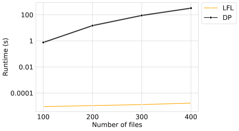
(b) Runtime (in seconds, logarithmic scale).

Figure 2: General performance on small synthetic instances (in color).

Figure 2-(b) illustrates the runtime of LFL and DP. Note that the other algorithms run in constant time and thereby are omitted from the plot. Times for DP are several orders of magnitude higher than that of LFL, requiring on average 107 seconds over all small instances. Thus, DP is not adequate in scenarios where the number of files grow considerably larger than 100 (see also §7.2).

For scalability purposes, we next investigate the performance on large-scale tape sizes in Figures 3-(a) and 3-(b).

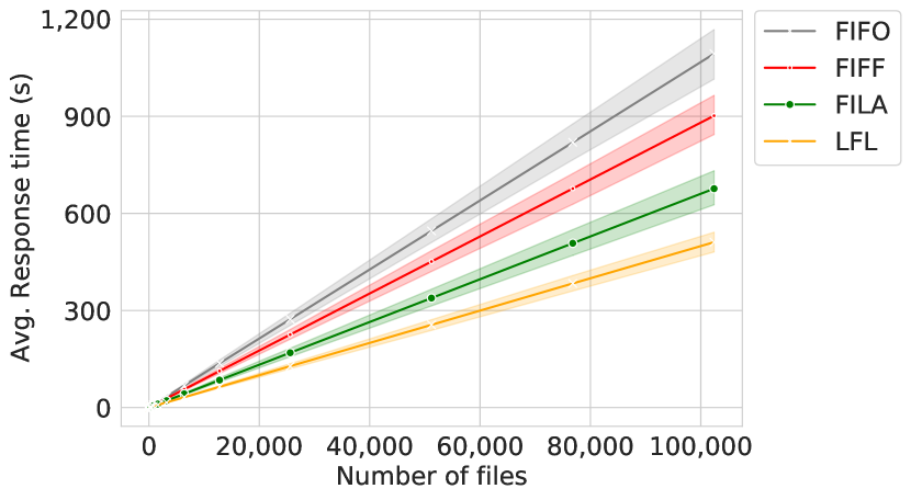
(a) Average response time per file.

(b) Runtime (in seconds, logarithmic scale).

Figure 3: General performance on large synthetic instances (in color).

The results in Figure 3-(a) show that the performance trend of the approximate policies remains the same as the number of files grow. LFL is consistently superior to the other policies, and its runtime (below 0.001 seconds) suggests that it is also practical.

Empirical Approximation.

Figures 4-(a) and 4-(b) depict the average approximation ratio as a function of the request probability $p$ and the standard deviation parameter $\sigma$ of the log-normal distribution, respectively, on the small synthetic instances. The shaded areas represent the 95% confidence intervals.

(a) Performance per request probability.

(b) Performance per file size deviation.

Figure 4: Approximation ratio under different request probabilities $p$ and file size deviations $\sigma$ regimes (in color).

The values are relative to the optimal solutions obtained by DP. FIFF is worse on instances with fewer requests, producing sequences having twice the optimal total response time for $p\leq 0.4$. This occurs because FIFF postpones files to the forward stage, and thus it may take a significant amount of time to read them after reaching position $0$. FILA, due to its symmetry to FIFF, has the opposite behavior and is preferable when there are few requests. The approximation ratio of all policies increases with the file deviation $\sigma$. FILA and LFL exhibit significantly better empirical performance than their theoretical worst case. In particular, LFL has a maximum approximation ratio of approximately $1.029$ over all instances. FIFO is outperformed by all approximate policies.

Value of File Access Frequency Data.

We next investigate the value of pre-fixing sequences in the presence of distributional information captured in the SLTS. We consider a single tape configuration with $n=250$ and file sizes drawn from a log-normal distribution with parameters $\mu=13.04$ and $\sigma=2.38$. For each $p\in\{0.2,0.4,0.6,0.8\}$, we solve the SLTS optimally assuming $p_{i}=p$ for all $i\in\mathscr{F}$ and evaluate the performance of the resulting sequence $\boldsymbol{\pi}_{p}$ for 100 runs, where each file is requested at random with probability $p$. In particular, we assume that files are skipped in $\boldsymbol{\pi}_{p}$ if they are not requested in the run. Figure 5 compares the performance of the resulting method, dubbed SLTS, with FIFO, FIFF, FILA, and LFL for each run. The results are aggregated by $p$ and normalized by the optimal solution obtained using DP.

(a) Performance per request probability.

(b) Performance of the SLTS.

Figure 5: Approximation ratio under different request probabilities $p$ (in color).

The average performance of SLTS is superior to all existing policies at $p\geq 0.4$, where the number of requests is medium to high. For smaller values of $p$, LFL outperforms SLTS by at most 20%. However, Figure 5-(b) suggests that larger gaps only occur for small values of $p$; otherwise, SLTS has strong overall performance. Notably, once $\boldsymbol{\pi}_{p}$ has been computed for the SLTS, adjusting the sequence for the requested files takes negligible time, thus making it more interesting in scenarios where the computational resources are severely restricted.

7.2 Landsat Instances

The Landsat program is a space mission that images the Earth’s surface every 16 days. Landsat 8, developed as a collaboration between NASA and the U.S. Geological Survey (USGS), is the eighth of the series of satellites launched by the mission. The images measure different ranges of frequencies (called “bands”) along the electromagnetic spectrum. Because the sensing process generates massive amounts of data, Landsat 8 data sets are split into a collection of tiles (or satellite scenes). Each tile is stored in a single file with approximately 3.5 GB of data and features 12 bands encoded by numerical pixel matrices. The files are used by machine learning algorithms to classify the health conditions of vineyards for precision viticulture purposes and include vineyards in the Atacama desert in Chile, the Serra Gaucha region in Brazil, and the Manduria region in Italy.

Our benchmark contains 100 instances with different configurations of the Landsat dataset. Every instance consists of 15 Landsat tiles, each composed of 12 files (and hence one file per band). The average file size is approximately 280 MB, with a small standard deviation (less than 1 MB).

Figure 6: Performance on different instances of the Landsat dataset (in color).

Figures 6-(a) and 6-(b) depict a cumulative performance profile of the approximation algorithms and DP, respectively, on the Landsat dataset. We omit the performance plots of FILA and DP in Figure 6-(a) because they are similar to LFL. In terms of the average response time, the policies can be divided into three different categories. FIFO delivers the worst results, with an average response time of 230 seconds (standard deviation of 19). FIFF is approximately 13% better than FIFO, with an average response time of 204 seconds (standard deviation of 13). The remaining policies reduce the objective values by almost 50%, with average response times of 118 seconds (standard deviation of 18). DP improves upon the other algorithms by hundredths of seconds. The solution time curves in Figure 6-(b) show that DP requires up to three seconds to solve these instances. The approximate policies are fast enough to be used in practice and provide sequences under $0.02$ seconds.

8 Conclusions

This paper investigates policies to retrieve files stored in tapes to minimize the total response time. We consider three versions of the problem. For the deterministic case, we present low-complexity policies with constant-factor approximation guarantees and introduce a polynomial-time algorithm based on dynamic programming. We also develop a fully polynomial approximation scheme for a stochastic version of the problem where request probabilities are available. Finally, we study an online variant where requests arrive in real time, presenting the first constant-factor competitive algorithm. Our numerical analysis of both synthetic and real-world tape settings suggests that FIFO, the standard policy in industry, is outperformed by other low-complexity methods and that policy decisions benefit when considering file access probabilities.

Appendix A Example

Consider a tape with five files, sizes $(s_{1},\dots,s_{5})=(2,2,8,2,1)$, and tape velocity of $\nu=1$ bit per time unit. The tape in Figure 7 depicts the sequence $\pi=(5,4,1,2,3)$, where solid (colored) arcs denote tape repositioning and dashed (black) arcs denote file reading operations as in Figure 1. For instance, to read file 4 (the second in the ordering), the tape header finishes reading file 1 at time 2, repositions itself to the left of file 4 at time 9 (since it must traverse boths files 4 and 5), and finishes reading the file at time 15. The response time of file $4$ is the time at which the tape head first started reading it, i.e., $9$. Note also that there is no need to reposition the tape header when reading file $2$ after file $1$. The total response time of $\pi$ is $R_{1}(\pi)+\dots+R_{5}(\pi)=1+5+21+23+25=75$.

Figure 7: Example of tape movement for the sequence $\boldsymbol{\pi}=(5,4,1,2,3)$.

Figure 8 illustrates a simpler policy (First-File-First, or FIFF) that moves the tape head to the beginning of the tape and reads files in sequence, i.e., $\boldsymbol{\pi}^{\prime}=(1,2,3,4,5)$. Its intuition is that the tape only requires to do a single left-to-right movement. The total response time of $\pi^{\prime}$ is $15+17+19+27+29=107$, i.e., 42% higher than from the sequence above. The difference is due to the presence of a large file with size 8, which must be traversed twice prior to reading files 4 and 5 in $\boldsymbol{\pi}^{\prime}$, increasing the response time. This is the basis of worst-case scenarios investigated in §4.

Figure 8: Example of tape movement for the sequence $\boldsymbol{\pi}^{\prime}=(1,2,3,4,5)$.

Appendix B Tables and Complementary Numerical Results

B.1 Synthethic Instances

Tables 1, 2, 3, 4, and 5 present the results of FIFO, FIFF, FILA, LFL, and DP, respectively, for synthethic instances. An entry corresponds to the average response time (in seconds, truncated to two decimal places) and the standard deviation (truncated to one decimal place) based on each configuration $(p,\sigma)$, where $p$ is the probability that a file in the tape is requested and $\sigma$ is the parameter of the log-normal distribution for file sizes (with $\mu=13.04$ for all cases). Each value is the mean of the 10 instances for the associated configuration. Due to memory and time limitations, we conducted experiments with DP using only small instances (with up to 400 files), so Table 5 has fewer columns than the others.

Table 1: Average response times - FIFO (in seconds).

Parameters		Small Instances				Large Instances
$p(\%)$	$\sigma$	100	200	300	400	800	1,600	3,200	6,400	12,800	25,600	51,200	76,800	102,400
25	1.50	0.4 (0.0)	0.84 (0.1)	1.29 (0.1)	1.74 (0.1)	3.57 (0.2)	7.13 (0.3)	14.69 (0.3)	28.76 (0.8)	57.98 (0.9)	116.48 (1.3)	348.36 (2.9)	234.08 (3.3)	465.83 (6.1)
25	2.00	0.64 (0.1)	1.3 (0.2)	1.9 (0.1)	2.6 (0.3)	5.68 (0.2)	11.04 (0.2)	22.69 (0.7)	44.57 (1.6)	90.25 (1.2)	180.28 (3.2)	541.9 (6.8)	361.5 (4.0)	725.54 (6.0)
25	2.38	0.87 (0.2)	1.85 (0.3)	3.03 (0.3)	3.94 (0.4)	7.92 (0.4)	16.25 (0.3)	32.59 (0.8)	64.99 (0.9)	132.47 (2.6)	266.76 (4.1)	787.18 (7.5)	525.47 (7.7)	1050.55 (19.8)
25	2.50	1.0 (0.2)	2.26 (0.3)	3.25 (0.3)	4.38 (0.4)	9.18 (0.8)	18.5 (1.1)	36.96 (1.7)	73.64 (1.6)	148.52 (2.2)	296.44 (3.3)	886.47 (10.5)	594.51 (7.0)	1191.59 (9.4)
25	3.00	1.69 (0.2)	3.7 (0.5)	5.42 (0.5)	7.38 (0.5)	15.47 (0.7)	30.81 (1.8)	63.74 (2.5)	125.09 (3.1)	251.81 (6.1)	505.91 (10.0)	1522.17 (22.2)	1016.58 (16.2)	2040.57 (23.3)
50	1.50	0.43 (0.0)	0.86 (0.1)	1.3 (0.1)	1.83 (0.1)	3.66 (0.2)	7.35 (0.3)	14.72 (0.4)	29.01 (0.4)	58.36 (1.0)	116.16 (2.1)	349.69 (3.3)	232.06 (1.7)	463.81 (6.1)
50	2.00	0.66 (0.1)	1.39 (0.1)	2.11 (0.3)	2.8 (0.2)	5.56 (0.3)	11.25 (0.4)	22.59 (0.5)	45.16 (0.8)	90.28 (1.5)	180.5 (2.7)	541.76 (6.8)	363.03 (4.5)	728.73 (5.7)
50	2.38	0.93 (0.2)	2.02 (0.2)	2.95 (0.3)	3.97 (0.4)	8.01 (0.5)	15.58 (0.7)	32.58 (0.5)	66.04 (0.6)	132.32 (2.2)	261.59 (6.0)	796.13 (6.5)	529.41 (4.7)	1060.76 (7.4)
50	2.50	1.11 (0.1)	2.11 (0.2)	3.57 (0.1)	4.55 (0.3)	9.12 (0.4)	18.54 (0.7)	36.9 (1.4)	74.36 (1.4)	149.45 (2.2)	297.37 (4.8)	892.11 (10.1)	592.5 (8.2)	1179.89 (9.6)
50	3.00	1.77 (0.3)	3.77 (0.5)	5.33 (0.5)	7.54 (0.7)	15.48 (1.0)	30.5 (1.6)	62.69 (2.8)	125.52 (3.6)	253.55 (6.6)	508.52 (7.4)	1526.99 (13.7)	1007.36 (13.6)	2031.28 (17.9)
75	1.50	0.43 (0.1)	0.91 (0.0)	1.37 (0.1)	1.79 (0.1)	3.57 (0.1)	7.32 (0.3)	14.23 (0.4)	29.27 (0.4)	58.3 (0.7)	117.1 (1.7)	348.38 (3.7)	232.02 (3.0)	468.05 (4.5)
75	2.00	0.67 (0.1)	1.33 (0.1)	2.08 (0.2)	2.84 (0.2)	5.65 (0.3)	11.17 (0.4)	22.47 (0.4)	44.85 (0.6)	90.49 (1.5)	180.61 (1.8)	542.67 (7.4)	362.46 (5.1)	725.88 (4.4)
75	2.38	1.02 (0.2)	2.06 (0.3)	2.95 (0.2)	4.07 (0.3)	8.01 (0.4)	16.11 (0.3)	32.53 (1.2)	65.49 (1.5)	131.51 (1.8)	262.44 (4.0)	785.32 (13.3)	525.57 (3.8)	1051.15 (11.1)
75	2.50	1.13 (0.2)	2.28 (0.3)	3.29 (0.3)	4.66 (0.5)	9.57 (0.6)	18.78 (0.6)	37.19 (1.2)	74.57 (1.3)	149.44 (1.5)	300.69 (2.9)	891.19 (10.6)	593.17 (8.5)	1190.18 (14.3)
75	3.00	1.9 (0.3)	4.11 (0.4)	5.73 (0.6)	8.14 (0.8)	15.24 (1.0)	31.12 (0.7)	62.38 (2.3)	126.82 (3.5)	253.87 (4.2)	504.67 (4.8)	1526.21 (17.8)	1014.08 (7.8)	2026.82 (17.8)
100	1.50	0.44 (0.1)	0.9 (0.1)	1.36 (0.1)	1.76 (0.1)	3.62 (0.2)	7.41 (0.2)	14.37 (0.4)	29.32 (0.5)	57.95 (0.8)	116.42 (1.1)	349.04 (3.3)	235.01 (1.3)	465.53 (4.5)
100	2.00	0.68 (0.1)	1.41 (0.1)	2.09 (0.2)	2.84 (0.2)	5.63 (0.3)	11.38 (0.4)	22.17 (0.4)	45.46 (0.7)	90.17 (1.2)	181.82 (2.2)	546.38 (7.3)	361.2 (4.4)	723.95 (7.0)
100	2.38	1.03 (0.2)	1.98 (0.3)	2.86 (0.3)	3.97 (0.3)	8.01 (0.4)	16.49 (0.8)	32.56 (1.7)	65.45 (1.3)	133.01 (2.7)	263.42 (4.2)	792.1 (7.0)	527.21 (8.3)	1059.02 (8.5)
100	2.50	1.07 (0.2)	2.18 (0.2)	3.42 (0.3)	4.61 (0.3)	8.96 (0.5)	18.89 (0.7)	37.09 (1.4)	74.4 (1.4)	148.98 (3.7)	296.87 (4.3)	891.42 (11.7)	596.85 (9.2)	1197.52 (9.7)
100	3.00	1.88 (0.4)	4.06 (0.6)	5.75 (0.3)	7.63 (0.8)	15.88 (0.7)	32.56 (1.3)	63.17 (2.7)	126.99 (3.7)	256.24 (6.0)	505.43 (7.5)	1522.9 (17.4)	1015.09 (13.3)	2022.33 (16.2)

Table 2: Average response time - FIFF (in seconds).

Parameters		Small Instances				Large Instances
$p(\%)$	$\sigma$	100	200	300	400	800	1,600	3,200	6,400	12,800	25,600	51,200	76,800	102,400
25	1.50	0.36 (0.0)	0.75 (0.1)	1.12 (0.1)	1.53 (0.1)	3.04 (0.1)	6.04 (0.2)	12.13 (0.2)	23.81 (0.5)	48.2 (0.5)	95.97 (0.5)	288.13 (1.3)	192.76 (1.1)	386.12 (0.8)
25	2.00	0.6 (0.1)	1.15 (0.1)	1.67 (0.1)	2.27 (0.2)	4.79 (0.2)	9.26 (0.3)	18.68 (0.4)	37.42 (0.9)	74.59 (0.9)	149.37 (1.6)	448.52 (3.1)	298.63 (1.8)	597.95 (1.9)
25	2.38	0.81 (0.1)	1.64 (0.2)	2.62 (0.3)	3.31 (0.3)	6.85 (0.3)	13.52 (0.3)	27.16 (0.7)	53.98 (0.6)	108.92 (1.5)	219.17 (2.2)	651.24 (3.3)	436.18 (2.9)	868.26 (4.3)
25	2.50	0.92 (0.2)	1.97 (0.3)	2.89 (0.3)	3.77 (0.4)	7.75 (0.7)	15.52 (1.0)	30.42 (0.9)	61.14 (1.2)	123.6 (1.7)	245.32 (2.8)	737.22 (4.9)	491.74 (3.6)	982.5 (3.9)
25	3.00	1.5 (0.2)	3.21 (0.3)	4.79 (0.6)	6.4 (0.5)	13.11 (0.5)	25.96 (1.1)	53.38 (1.8)	103.9 (2.2)	209.67 (5.1)	418.97 (5.1)	1257.22 (12.2)	839.29 (7.1)	1676.04 (11.0)
50	1.50	0.37 (0.0)	0.73 (0.0)	1.1 (0.1)	1.53 (0.1)	3.03 (0.1)	6.12 (0.2)	12.2 (0.3)	23.93 (0.4)	48.17 (0.4)	96.28 (0.8)	287.91 (1.1)	192.27 (1.3)	384.85 (1.6)
50	2.00	0.59 (0.1)	1.18 (0.1)	1.83 (0.2)	2.34 (0.2)	4.61 (0.3)	9.36 (0.2)	18.81 (0.4)	37.22 (0.6)	74.64 (0.5)	149.37 (1.3)	447.71 (2.6)	300.06 (1.5)	598.31 (3.4)
50	2.38	0.81 (0.1)	1.75 (0.1)	2.58 (0.3)	3.39 (0.4)	6.71 (0.4)	13.06 (0.6)	26.96 (0.6)	54.16 (0.5)	108.49 (1.3)	217.13 (2.9)	653.28 (3.7)	434.89 (2.5)	869.02 (4.8)
50	2.50	0.96 (0.1)	1.78 (0.2)	3.0 (0.2)	3.86 (0.3)	7.69 (0.5)	15.33 (0.6)	30.59 (1.0)	61.41 (0.9)	123.11 (1.6)	245.95 (2.7)	737.44 (2.9)	491.24 (2.9)	979.62 (4.1)
50	3.00	1.53 (0.3)	3.24 (0.4)	4.51 (0.5)	6.41 (0.6)	13.11 (0.7)	25.1 (1.4)	52.02 (1.8)	104.25 (2.6)	209.35 (3.4)	418.48 (4.0)	1257.83 (6.0)	837.24 (6.8)	1672.09 (11.4)
75	1.50	0.36 (0.0)	0.77 (0.0)	1.15 (0.1)	1.51 (0.1)	2.99 (0.1)	6.03 (0.2)	11.85 (0.2)	24.12 (0.3)	48.19 (0.3)	96.56 (0.6)	288.39 (1.1)	192.26 (0.9)	384.9 (0.7)
75	2.00	0.57 (0.1)	1.16 (0.1)	1.76 (0.1)	2.36 (0.1)	4.71 (0.2)	9.24 (0.3)	18.55 (0.3)	37.19 (0.6)	74.59 (1.1)	149.09 (1.5)	449.01 (2.1)	298.6 (2.2)	598.39 (3.0)
75	2.38	0.84 (0.1)	1.78 (0.2)	2.45 (0.2)	3.38 (0.2)	6.62 (0.3)	13.34 (0.5)	26.91 (1.0)	54.06 (0.8)	108.4 (1.0)	216.27 (1.9)	650.15 (3.7)	433.99 (1.9)	870.44 (3.2)
75	2.50	1.0 (0.2)	1.93 (0.2)	2.78 (0.3)	3.84 (0.3)	7.94 (0.5)	15.72 (0.4)	30.6 (1.0)	61.85 (1.4)	123.26 (1.4)	246.05 (1.3)	738.06 (5.5)	490.27 (3.5)	980.84 (4.4)
75	3.00	1.63 (0.3)	3.47 (0.3)	4.72 (0.4)	6.83 (0.7)	12.75 (0.8)	26.3 (0.7)	51.91 (1.7)	104.39 (2.3)	208.17 (2.3)	419.61 (4.3)	1260.37 (7.4)	837.47 (7.3)	1671.08 (9.9)
100	1.50	0.38 (0.0)	0.77 (0.1)	1.14 (0.1)	1.46 (0.1)	3.02 (0.1)	6.11 (0.2)	11.96 (0.3)	24.15 (0.3)	47.96 (0.3)	96.04 (0.8)	288.74 (1.3)	192.82 (1.0)	384.58 (1.5)
100	2.00	0.58 (0.1)	1.16 (0.1)	1.76 (0.2)	2.4 (0.2)	4.65 (0.2)	9.42 (0.4)	18.35 (0.4)	37.55 (0.5)	75.01 (0.5)	149.88 (1.1)	449.87 (4.4)	298.37 (2.9)	598.48 (3.5)
100	2.38	0.86 (0.2)	1.65 (0.2)	2.38 (0.2)	3.37 (0.2)	6.62 (0.3)	13.54 (0.6)	27.15 (1.3)	53.85 (0.8)	109.06 (1.7)	216.9 (2.2)	652.28 (4.7)	435.55 (4.1)	871.17 (3.4)
100	2.50	0.92 (0.1)	1.81 (0.2)	2.83 (0.2)	3.85 (0.3)	7.43 (0.4)	15.74 (0.6)	30.55 (0.9)	61.79 (1.3)	123.4 (2.0)	244.96 (2.3)	737.2 (4.1)	491.43 (4.4)	983.18 (5.0)
100	3.00	1.59 (0.3)	3.44 (0.5)	4.85 (0.3)	6.42 (0.6)	13.15 (0.7)	26.59 (1.0)	52.22 (2.3)	105.02 (2.8)	211.26 (3.6)	418.43 (4.6)	1254.62 (7.6)	838.35 (7.9)	1677.34 (9.6)

Table 3: Average response time - FILA (in seconds).

Parameters		Small Instances				Large Instances
$p(\%)$	$\sigma$	100	200	300	400	800	1,600	3,200	6,400	12,800	25,600	51,200	76,800	102,400
25	1.50	0.19 (0.04)	0.36 (0.05)	0.58 (0.04)	0.76 (0.04)	1.53 (0.11)	2.97 (0.11)	6.13 (0.13)	11.91 (0.26)	23.97 (0.26)	47.96 (0.46)	143.72 (0.74)	96.51 (1.04)	192.36 (0.47)
25	2.00	0.32 (0.04)	0.59 (0.13)	0.85 (0.07)	1.14 (0.14)	2.36 (0.12)	4.71 (0.22)	9.26 (0.21)	18.74 (0.74)	37.38 (0.75)	74.45 (1.41)	225.33 (2.23)	149.71 (1.6)	297.96 (1.49)
25	2.38	0.4 (0.11)	0.77 (0.14)	1.32 (0.17)	1.73 (0.24)	3.46 (0.25)	6.77 (0.22)	13.3 (0.49)	27.03 (0.39)	54.92 (1.17)	109.54 (1.32)	324.53 (1.6)	218.31 (2.13)	434.73 (3.52)
25	2.50	0.48 (0.15)	1.02 (0.23)	1.42 (0.22)	1.89 (0.23)	4.0 (0.45)	7.93 (0.51)	15.58 (0.9)	30.62 (0.68)	61.69 (0.95)	122.59 (1.46)	367.07 (3.01)	244.46 (2.45)	492.17 (3.24)
25	3.00	0.77 (0.17)	1.71 (0.22)	2.54 (0.4)	3.38 (0.24)	6.57 (0.47)	12.98 (0.64)	26.63 (1.04)	51.3 (1.7)	103.79 (1.34)	209.25 (4.34)	629.61 (5.27)	419.58 (4.78)	839.61 (6.21)
50	1.50	0.25 (0.03)	0.51 (0.04)	0.75 (0.06)	1.03 (0.05)	2.06 (0.11)	4.0 (0.17)	8.08 (0.23)	16.0 (0.25)	32.08 (0.34)	64.09 (0.87)	192.04 (1.04)	127.99 (0.8)	256.89 (1.1)
50	2.00	0.38 (0.08)	0.8 (0.07)	1.21 (0.14)	1.61 (0.1)	3.15 (0.26)	6.28 (0.3)	12.53 (0.15)	24.93 (0.6)	49.81 (0.59)	99.44 (1.29)	298.97 (1.77)	199.93 (1.36)	399.21 (1.13)
50	2.38	0.51 (0.1)	1.13 (0.12)	1.69 (0.18)	2.31 (0.27)	4.5 (0.34)	8.87 (0.29)	17.94 (0.27)	36.01 (0.95)	72.79 (1.65)	144.15 (2.13)	436.17 (2.57)	289.05 (2.86)	579.4 (4.3)
50	2.50	0.6 (0.12)	1.13 (0.23)	2.07 (0.16)	2.59 (0.35)	5.08 (0.28)	10.18 (0.64)	20.49 (0.85)	40.66 (1.33)	83.22 (0.79)	164.16 (2.18)	491.89 (3.01)	326.64 (2.37)	653.87 (4.97)
50	3.00	0.96 (0.24)	2.23 (0.46)	3.12 (0.5)	4.26 (0.57)	8.63 (0.79)	17.05 (1.17)	34.85 (1.66)	69.75 (1.56)	138.78 (2.86)	280.94 (2.73)	839.18 (8.76)	556.21 (6.99)	1115.11 (9.63)
75	1.50	0.31 (0.04)	0.62 (0.04)	0.94 (0.08)	1.25 (0.1)	2.49 (0.09)	5.01 (0.22)	9.84 (0.23)	20.04 (0.34)	40.17 (0.48)	80.55 (0.64)	240.57 (1.34)	159.78 (1.28)	321.13 (0.99)
75	2.00	0.44 (0.09)	0.93 (0.12)	1.41 (0.14)	1.98 (0.18)	3.85 (0.23)	7.67 (0.24)	15.53 (0.35)	30.76 (0.4)	62.07 (0.85)	124.46 (1.03)	373.19 (2.23)	248.7 (2.17)	498.42 (2.86)
75	2.38	0.72 (0.16)	1.46 (0.15)	2.07 (0.12)	2.84 (0.3)	5.61 (0.3)	11.11 (0.38)	22.42 (1.03)	45.42 (1.34)	90.99 (1.44)	179.84 (1.95)	541.38 (4.44)	362.05 (2.9)	724.47 (2.44)
75	2.50	0.8 (0.14)	1.61 (0.23)	2.41 (0.26)	3.32 (0.27)	6.66 (0.41)	12.91 (0.64)	25.72 (1.02)	51.26 (1.12)	102.55 (1.9)	206.43 (2.51)	613.65 (4.91)	409.13 (2.26)	817.27 (4.48)
75	3.00	1.35 (0.31)	2.9 (0.45)	4.13 (0.52)	5.83 (0.44)	10.54 (1.05)	21.81 (0.72)	43.53 (1.87)	86.79 (2.92)	174.76 (2.68)	351.24 (4.49)	1052.72 (7.89)	698.67 (7.62)	1394.4 (9.3)
100	1.50	0.38 (0.05)	0.73 (0.07)	1.15 (0.06)	1.47 (0.08)	3.02 (0.15)	6.13 (0.19)	12.01 (0.42)	24.11 (0.4)	47.96 (0.42)	95.88 (0.78)	288.88 (1.04)	192.52 (1.07)	384.64 (1.61)
100	2.00	0.57 (0.12)	1.2 (0.1)	1.75 (0.18)	2.37 (0.16)	4.68 (0.33)	9.4 (0.51)	18.42 (0.42)	37.8 (0.55)	75.0 (0.93)	150.0 (1.39)	450.28 (3.68)	298.01 (3.35)	597.9 (3.62)
100	2.38	0.86 (0.22)	1.73 (0.24)	2.5 (0.37)	3.3 (0.17)	6.76 (0.36)	13.45 (0.56)	27.06 (1.52)	54.15 (1.35)	109.29 (1.71)	216.55 (2.49)	653.67 (4.54)	434.72 (4.71)	870.3 (4.72)
100	2.50	0.86 (0.11)	1.87 (0.19)	2.87 (0.24)	3.85 (0.35)	7.52 (0.54)	15.48 (0.63)	30.45 (1.28)	61.68 (0.99)	123.17 (2.65)	246.07 (2.51)	736.54 (4.5)	492.22 (5.41)	983.42 (6.66)
100	3.00	1.64 (0.35)	3.27 (0.46)	4.69 (0.33)	6.47 (0.73)	13.2 (0.8)	27.17 (1.24)	52.22 (2.32)	104.46 (2.81)	212.1 (3.3)	418.58 (4.87)	1254.78 (7.94)	841.76 (8.21)	1676.29 (12.15)

Table 4: Average response time - LFL (in seconds).

Parameters		Small Instances				Large Instances
$p(\%)$	$\sigma$	100	200	300	400	800	1,600	3,200	6,400	12,800	25,600	51,200	76.800	102,400
25	1.50	0.19 (0.0)	0.36 (0.1)	0.58 (0.0)	0.76 (0.0)	1.53 (0.1)	2.97 (0.1)	6.13 (0.1)	11.91 (0.3)	23.97 (0.3)	47.96 (0.5)	143.72 (0.7)	96.51 (1.0)	192.36 (0.5)
25	2.00	0.31 (0.0)	0.59 (0.1)	0.84 (0.1)	1.14 (0.1)	2.36 (0.1)	4.7 (0.2)	9.26 (0.2)	18.74 (0.7)	37.38 (0.7)	74.44 (1.4)	225.33 (2.2)	149.71 (1.6)	297.96 (1.5)
25	2.38	0.39 (0.1)	0.75 (0.1)	1.29 (0.2)	1.69 (0.2)	3.42 (0.2)	6.7 (0.2)	13.19 (0.5)	26.69 (0.3)	54.47 (1.2)	108.71 (1.4)	321.42 (2.9)	216.88 (2.5)	431.17 (4.4)
25	2.50	0.47 (0.1)	0.98 (0.2)	1.38 (0.2)	1.85 (0.2)	3.92 (0.5)	7.75 (0.5)	15.24 (0.9)	30.02 (0.7)	60.84 (1.0)	120.55 (1.7)	361.68 (4.7)	240.18 (2.4)	483.73 (3.8)
25	3.00	0.73 (0.2)	1.64 (0.2)	2.39 (0.3)	3.22 (0.2)	6.27 (0.4)	12.43 (0.7)	25.47 (1.0)	49.2 (1.6)	99.73 (1.5)	200.34 (4.1)	603.77 (5.7)	402.52 (4.2)	804.97 (5.8)
50	1.50	0.23 (0.0)	0.46 (0.0)	0.69 (0.1)	0.96 (0.0)	1.92 (0.1)	3.75 (0.2)	7.53 (0.2)	14.87 (0.2)	29.89 (0.3)	59.68 (0.8)	178.82 (0.8)	119.24 (0.8)	239.18 (1.1)
50	2.00	0.33 (0.1)	0.7 (0.1)	1.06 (0.1)	1.39 (0.1)	2.71 (0.2)	5.49 (0.2)	10.94 (0.2)	21.72 (0.5)	43.46 (0.5)	86.88 (1.0)	260.8 (1.5)	174.77 (1.1)	348.92 (1.2)
50	2.38	0.44 (0.1)	0.96 (0.1)	1.43 (0.2)	1.93 (0.2)	3.75 (0.3)	7.33 (0.3)	14.98 (0.3)	30.22 (0.6)	60.88 (1.3)	120.8 (1.9)	365.11 (2.3)	242.34 (2.1)	485.11 (3.3)
50	2.50	0.51 (0.1)	0.94 (0.2)	1.7 (0.1)	2.13 (0.2)	4.21 (0.3)	8.44 (0.5)	16.94 (0.8)	33.74 (0.8)	68.49 (0.9)	135.73 (1.9)	407.12 (2.0)	270.52 (1.8)	540.64 (3.3)
50	3.00	0.77 (0.2)	1.76 (0.3)	2.41 (0.4)	3.35 (0.4)	6.85 (0.5)	13.38 (0.9)	27.49 (1.3)	54.91 (1.5)	110.17 (2.1)	222.03 (2.2)	664.82 (6.4)	441.32 (4.7)	883.26 (8.0)
75	1.50	0.25 (0.0)	0.52 (0.0)	0.78 (0.1)	1.04 (0.1)	2.06 (0.1)	4.15 (0.2)	8.16 (0.2)	16.6 (0.2)	33.28 (0.4)	66.72 (0.5)	199.25 (0.9)	132.54 (0.8)	265.77 (0.7)
75	2.00	0.35 (0.1)	0.71 (0.1)	1.09 (0.1)	1.49 (0.1)	2.94 (0.1)	5.85 (0.2)	11.76 (0.2)	23.47 (0.4)	47.24 (0.6)	94.63 (0.7)	284.16 (1.7)	189.19 (1.6)	379.16 (1.8)
75	2.38	0.52 (0.1)	1.04 (0.1)	1.49 (0.1)	2.02 (0.2)	4.03 (0.2)	8.0 (0.3)	16.14 (0.7)	32.65 (0.8)	65.43 (0.9)	129.8 (1.3)	390.17 (2.6)	260.88 (1.5)	522.32 (1.8)
75	2.50	0.58 (0.1)	1.13 (0.2)	1.67 (0.2)	2.31 (0.2)	4.72 (0.3)	9.21 (0.4)	18.22 (0.7)	36.5 (0.8)	72.93 (1.3)	146.15 (1.3)	436.39 (3.3)	290.16 (1.8)	579.93 (2.8)
75	3.00	0.93 (0.2)	1.95 (0.2)	2.73 (0.3)	3.91 (0.4)	7.06 (0.6)	14.64 (0.4)	29.27 (1.2)	58.43 (1.7)	117.26 (1.6)	235.85 (2.8)	706.83 (4.7)	469.5 (5.1)	936.65 (6.2)
100	1.50	0.28 (0.0)	0.55 (0.0)	0.84 (0.0)	1.08 (0.1)	2.25 (0.1)	4.53 (0.1)	8.85 (0.3)	17.9 (0.3)	35.41 (0.3)	70.95 (0.5)	213.53 (0.9)	142.51 (0.9)	284.36 (1.1)
100	2.00	0.39 (0.1)	0.78 (0.1)	1.18 (0.1)	1.59 (0.1)	3.13 (0.2)	6.32 (0.3)	12.32 (0.3)	25.34 (0.4)	50.4 (0.5)	100.8 (0.9)	302.39 (2.8)	200.25 (2.3)	402.0 (2.3)
100	2.38	0.54 (0.1)	1.07 (0.2)	1.55 (0.2)	2.12 (0.1)	4.21 (0.2)	8.58 (0.4)	17.12 (0.9)	34.1 (0.7)	69.08 (1.2)	137.24 (1.5)	413.1 (2.9)	275.28 (3.0)	550.55 (2.8)
100	2.50	0.55 (0.1)	1.15 (0.1)	1.74 (0.2)	2.38 (0.2)	4.65 (0.3)	9.7 (0.4)	18.95 (0.7)	38.35 (0.8)	76.59 (1.6)	152.62 (1.6)	458.0 (2.7)	305.8 (3.2)	611.96 (3.6)
100	3.00	0.95 (0.2)	1.95 (0.3)	2.74 (0.2)	3.8 (0.4)	7.7 (0.5)	15.91 (0.7)	30.4 (1.4)	61.26 (1.8)	123.86 (1.9)	244.44 (3.2)	733.35 (4.4)	491.18 (5.1)	979.49 (7.5)

Table 5: Average response times - DP (in seconds).

Parameters		Small Instances
$p(\%)$	$\sigma$	100	200	300	400
25	1.50	0.19 (0.0)	0.36 (0.1)	0.58 (0.0)	0.75 (0.0)
25	2.00	0.31 (0.0)	0.59 (0.1)	0.84 (0.1)	1.13 (0.1)
25	2.38	0.39 (0.1)	0.75 (0.1)	1.29 (0.2)	1.69 (0.2)
25	2.50	0.47 (0.1)	0.98 (0.2)	1.38 (0.2)	1.85 (0.2)
25	3.00	0.72 (0.2)	1.63 (0.2)	2.39 (0.3)	3.21 (0.2)
50	1.50	0.23 (0.0)	0.46 (0.0)	0.69 (0.1)	0.96 (0.0)
50	2.00	0.33 (0.1)	0.7 (0.1)	1.06 (0.1)	1.39 (0.1)
50	2.38	0.44 (0.1)	0.96 (0.1)	1.42 (0.2)	1.93 (0.2)
50	2.50	0.51 (0.1)	0.94 (0.2)	1.7 (0.1)	2.13 (0.2)
50	3.00	0.77 (0.2)	1.76 (0.3)	2.41 (0.4)	3.35 (0.4)
75	1.50	0.25 (0.0)	0.52 (0.0)	0.78 (0.1)	1.04 (0.1)
75	2.00	0.35 (0.1)	0.71 (0.1)	1.09 (0.1)	1.49 (0.1)
75	2.38	0.52 (0.1)	1.04 (0.1)	1.49 (0.1)	2.02 (0.2)
75	2.50	0.57 (0.1)	1.13 (0.2)	1.67 (0.2)	2.31 (0.2)
75	3.00	0.92 (0.2)	1.95 (0.2)	2.73 (0.3)	3.91 (0.4)
100	1.50	0.28 (0.0)	0.55 (0.0)	0.84 (0.0)	1.08 (0.1)
100	2.00	0.39 (0.1)	0.78 (0.1)	1.18 (0.1)	1.59 (0.1)
100	2.38	0.54 (0.1)	1.07 (0.2)	1.55 (0.2)	2.12 (0.1)
100	2.50	0.55 (0.1)	1.15 (0.1)	1.74 (0.2)	2.38 (0.2)
100	3.00	0.94 (0.2)	1.94 (0.3)	2.74 (0.2)	3.79 (0.4)

Table 6 reports the average runtime and respective standard deviation of DP and LFL (also in seconds, with two decimal places for the average and one for the standard deviation) based on each configuration $(p,\sigma)$. We omit the runtime of LFL for instances with less than 12,800 files as well as the runtime of all the other algorithms because these values are negligibly small. Moreover, the standard deviation for LFL is always equal to zero when truncated to two decimal places, so we omit this information from Table 6 as well.

Table 6: Average runtime - LFL and DP (in seconds).

Parameters		DP				LFL
$p(\%)$	$\sigma$	100	200	300	400	12,800	25,600	51,200	76,800	102,400
25	1.50	0.028 (0.02)	0.597 (0.21)	3.22 (2.37)	10.438 (3.39)	0.0	0.001	0.002	0.001	0.002
25	2.00	0.047 (0.03)	0.599 (0.31)	3.343 (1.05)	11.437 (3.31)	0.0	0.001	0.002	0.001	0.003
25	2.38	0.034 (0.02)	0.508 (0.26)	3.766 (1.89)	10.125 (4.21)	0.0	0.001	0.002	0.001	0.003
25	2.50	0.032 (0.03)	0.604 (0.15)	3.303 (1.91)	9.57 (4.0)	0.0	0.001	0.002	0.002	0.003
25	3.00	0.051 (0.03)	0.488 (0.15)	3.212 (1.12)	10.841 (2.8)	0.0	0.001	0.002	0.002	0.003
50	1.50	0.335 (0.11)	6.968 (1.13)	36.842 (10.59)	134.96 (27.24)	0.001	0.001	0.004	0.002	0.005
50	2.00	0.342 (0.13)	5.816 (1.18)	37.434 (10.55)	141.646 (28.48)	0.001	0.001	0.004	0.002	0.005
50	2.38	0.344 (0.1)	5.701 (0.96)	39.338 (5.67)	124.112 (33.33)	0.001	0.001	0.003	0.002	0.005
50	2.50	0.33 (0.12)	5.228 (0.91)	40.472 (11.89)	128.625 (23.31)	0.001	0.001	0.003	0.002	0.005
50	3.00	0.325 (0.14)	5.837 (1.84)	42.639 (9.65)	125.374 (17.22)	0.0	0.001	0.003	0.002	0.004
75	1.50	1.019 (0.06)	19.309 (2.58)	117.204 (9.28)	419.384 (45.4)	0.001	0.001	0.004	0.002	0.005
75	2.00	0.939 (0.17)	19.322 (2.65)	119.615 (12.32)	434.223 (33.8)	0.001	0.001	0.004	0.002	0.005
75	2.38	1.054 (0.08)	20.058 (2.28)	114.735 (13.43)	437.175 (35.62)	0.001	0.001	0.004	0.002	0.005
75	2.50	1.019 (0.16)	19.505 (1.3)	117.44 (7.08)	423.632 (28.27)	0.001	0.001	0.003	0.002	0.005
75	3.00	1.014 (0.16)	20.896 (2.4)	117.295 (8.46)	442.009 (44.0)	0.0	0.001	0.003	0.002	0.004
100	1.50	1.646 (0.01)	32.932 (0.18)	196.048 (0.63)	725.787 (5.38)	0.001	0.001	0.004	0.002	0.005
100	2.00	1.644 (0.01)	32.939 (0.16)	196.853 (1.47)	724.231 (4.9)	0.0	0.001	0.003	0.002	0.004
100	2.38	1.648 (0.01)	33.173 (0.85)	195.943 (0.97)	723.494 (4.57)	0.0	0.001	0.003	0.002	0.004
100	2.50	1.646 (0.01)	33.401 (1.61)	195.61 (0.58)	724.318 (7.0)	0.0	0.001	0.003	0.002	0.004
100	3.00	1.653 (0.02)	32.804 (0.06)	196.289 (0.93)	726.582 (11.72)	0.0	0.001	0.003	0.002	0.004

Table 7 compares the average quality of the solution produced by each algorithm, given by the ratio between the solution produced by the algorithm and the optimal solution identified by DP. LFL delivers solid performance, as observed in the other experiments, but we observe that its advantage of SLTS gets reduced as the percentage with which files are requested decreases.

Table 7: Average approximation ratio of each algorithm on stochastic instances in comparison with DP.

$p(\%)$	Algorithm
	FIFO	FIFF	FILA	LFL	SLTS
20	2.35 (0.2)	2.06 (0.2)	1.01 (0.0)	1.0 (0.0)	1.21 (0.1)
40	2.07 (0.1)	1.77 (0.1)	1.11 (0.0)	1.0 (0.0)	1.07 (0.0)
60	1.94 (0.1)	1.64 (0.1)	1.26 (0.0)	1.0 (0.0)	1.02 (0.0)
80	1.87 (0.0)	1.56 (0.0)	1.41 (0.0)	1.01 (0.0)	1.01 (0.0)
100	1.83 (0.0)	1.51 (0.0)	1.58 (0.0)	1.01 (0.0)	1.0 (0.0)

B.2 Landsat Instances

For the real-world tape settings, we consider a case study on the use of remote sensing for precision viticulture in 3 zones of interest: the Atacama desert in Chile, the Serra Gaucha region in Brazil, and the Manduria region in Italy. The Atacama region is represented by a cluster of 4 Landsat-8 tiles, and it is known for its dry weather and a mostly cloud-free sky all year round, which translates into crisp satellite imagery. The software accessing these tiles computes the Normalized Difference Vegetation Index (NDVI) of the region by reading Landsat bands number 4 and 5, which represent the reflective radiation in visible Red and Near-Infrared wavelengths, respectively. Differently from the Atacama region, Serra Gaucha and Manduria are frequently covered with clouds that, at times, invalidate whole satellite scenes [NASA, 2017]. The Serra Gaucha region is covered by 6 Landsat-8 tiles that, once processed, are converted into false-color images that emphasize vegetation; the image composition procedure used in this application requires the use of bands number 4, 5, and 6. Last, Manduria is composed of five tiles. The associated application uses a neural network that processes the assembled data to classify the vineyards’ health conditions.

Each aforementioned region is analysed by a different software, but in all cases read requests are contingent on the analysis of the QA band. If an image has a cloud cover above a certain threshold, then no bands other than the QA are read; the missing data is then interpolated or extrapolated at a later time using data from past and future scenes. This aspect is important, as cloud cover thresholds have a direct impact on read requests. Our experiments involve only the second stage of this pipeline, i.e., we assume that the QA bands have been inspected already and that all read requests involve spectrum bands of images that satisfy the cloud cover conditions.

The results of our experiments involving the Landsat instances are presented in Table 8. Each instance is associated with a configuration $(\alpha,\beta,\gamma)$; numbers $\alpha$, $\beta$, and $\gamma$ belong to the interval $[0,100]$ and indicate the threshold for cloud covers adopted by the applications using data associated with the Atacama, Serra Gaucha, and Manduria region, respectively. The data set has 10 instances for each of the following configurations of $(\alpha,\beta,\gamma)$: (2,15,22), (17,15,32), (7,21,22), (9,18,38), (17,21,32), (9,15,22), (2,26,38), (17,21,22), (2,21,22), and (17,26,38). The first column in the table indicates the configuration $\alpha-\beta-\gamma$, and each entry reports the average response times (in seconds) and respective standard deviations obtained by each algorithm over the 10 instances using two decimal places for the average and one for the standard deviation).

Table 8: Average response times for Landsat instances (in seconds).

Instance	Algorithm
$\alpha-\beta-\gamma$	FIFO	FIFF	FILA	LFL	DP
02-15-22	237.46 (16.2)	208.07 (13.8)	127.19 (21.9)	127.19 (21.9)	127.19 (21.9)
16-15-32	221.34 (12.9)	211.54 (11.0)	103.07 (16.6)	103.07 (16.6)	103.07 (16.6)
07-21-22	221.82 (18.6)	204.93 (15.1)	115.7 (8.8)	115.7 (8.8)	115.7 (8.8)
09-18-38	235.87 (20.7)	204.64 (14.7)	115.85 (14.9)	115.85 (14.9)	115.84 (14.9)
17-21-32	228.6 (23.8)	201.98 (16.7)	119.2 (16.0)	119.2 (16.0)	119.2 (16.0)
09-15-22	226.28 (16.7)	201.13 (9.1)	131.4 (21.4)	131.4 (21.4)	131.4 (21.4)
02-26-38	224.83 (23.4)	200.44 (11.2)	108.49 (18.4)	108.49 (18.4)	108.49 (18.4)
17-21-22	235.41 (13.3)	209.43 (11.7)	116.59 (18.1)	116.59 (18.1)	116.59 (18.1)
02-21-22	231.84 (15.2)	198.67 (10.2)	122.83 (13.9)	122.83 (13.9)	122.83 (13.9)
17-26-38	227.12 (23.0)	198.34 (15.6)	118.09 (14.0)	118.09 (14.0)	118.08 (14.0)

Appendix C Proofs

For ease of reference, we organize the proofs following the structure of the manuscript.

C.1 The LTS with Deterministic Service Requests

We use the following auxiliary lemma for the results below.

Lemma 2.

Suppose all files have the same size, i.e., $s_{i}=s$ for all $i\in\mathscr{F}$. Given an arbitrary set of requested files, there exists an optimal solution $\boldsymbol{\pi}^{*}$ such that $\pi^{*}_{t}>\pi^{*}_{t+1}$ for any rewind-stage file $\pi^{*}_{t}\in\mathcal{R}_{\boldsymbol{\pi}^{*}}$, $t<n$. That is, files in the rewind stage are read in descending order of their indices.

Proof.

Proof of Lemma 2. Let $\boldsymbol{\pi}$ be a solution to the LTS with a (non-necessarily contiguous) subsequence $(\pi_{t},\ldots,\pi_{t+k})$, $k\geq 1$, of rewind-stage files such that $\pi_{t}<\ldots<\pi_{t+k}$, i.e., they are read in ascending order in $\boldsymbol{\pi}$. We can assume $w_{\pi_{t}}=w_{\pi_{t+k}}=1$; otherwise, both files could be delayed to the forward stage without impacting the objective of the LTS. Since the tape head starts at position $L$, the file $\pi_{t+k}$ is eventually traversed from right to left at some moment prior to reading $\pi_{t}$. Create a new sequence $\boldsymbol{\pi}^{\prime}$ where $\pi_{t+k}$ is read immediately after the last-serviced file $\pi_{t^{\prime}}$ prior to reaching $\ell_{\pi_{t+k}}$ for the first time, where $t^{\prime}<t$; observe that such a file must exist, as we would have $\pi_{1}=\pi_{t}$ otherwise, thus contradicting the assumption that $\pi_{t}$ is a rewind-stage file.

The response time of each of the $k-1$ files $(\pi_{t},\ldots,\pi_{t+k-1})$ in $\boldsymbol{\pi}^{\prime}$ increases by $2s$ with respect to $\boldsymbol{\pi}$. Thus, the increase in the response time for reading these $k-1$ files is at most $2s(k-1)$ in $\boldsymbol{\pi}^{\prime}$, or potentially less if any of such files is not requested. Conversely, the response time of $\pi_{t+k}$ in $\boldsymbol{\pi}^{\prime}$ decreases by at least $2s(k-1)$, or more if the subsequence $(\pi_{t},\ldots,\pi_{t+k})$ is not contiguous. Since the response times of the files read after before $\pi_{t}$ or after $\pi_{t+k}$ do not change, the objective value of $\boldsymbol{\pi}^{\prime}$ is smaller than or equal to $\boldsymbol{\pi}$. The result follows from the iterative application of this argument on any optimal solution $\boldsymbol{\pi}^{*}$ to the LTS. $\blacksquare$ ∎

Proof.

Proof of Proposition 1. Let $\boldsymbol{\pi}^{*}$ be an optimal solution to the LTS that violates the condition of the statement, i.e., there exist indices $t<t^{\prime}$ such that $\pi^{*}_{t},\pi^{*}_{t^{\prime}}\in\mathcal{F}_{\boldsymbol{\pi}^{*}}$ and $\pi^{*}_{t}>\pi^{*}_{t^{\prime}}$. By definition, $1\in\mathcal{F}_{\boldsymbol{\pi}^{*}}$, which implies that the tape head must traverse $\pi^{*}_{t^{\prime}}$ from left to right prior to reading $\pi^{*}_{t}$. Suppose that such a traversal happens first between two forward-stage files $\pi^{*}_{\hat{t}}$ and $\pi^{*}_{\hat{t}+1}$ that are read consecutively in $\boldsymbol{\pi}^{*}$. Notice that we must have $\hat{t},\hat{t}+1\leq t$ and $\pi^{*}_{\hat{t}}<\pi^{*}_{\hat{t}+1}$, as $\pi^{*}_{t^{\prime}}$ is traversed from left to right. If we replace the contiguous subsequence $\dots,\pi^{*}_{\hat{t}},\pi^{*}_{\hat{t}+1},\dots$ in $\boldsymbol{\pi}^{*}$ by

$$\dots,\pi^{*}_{\hat{t}},\pi^{*}_{t^{\prime}},\pi^{*}_{\hat{t}+1},\dots$$

that is, we read $\pi^{*}_{t^{\prime}}$ the first time it is traversed from left to right, the response time of $\pi^{*}_{t^{\prime}}$ decreases if $w_{\pi^{*}_{t^{\prime}}}=1$. Moreover, the response times of the files that precede $\pi^{*}_{t^{\prime}}$ in $\boldsymbol{\pi}^{*}$ do not change, while the response times for the files that succeed $\pi^{*}_{t^{\prime}}$ in $\boldsymbol{\pi}^{*}$ can only decrease since there is no need to rewind the tape to $\ell_{\pi^{*}_{t^{\prime}}}$. Thus, the total response time either remains the same or decreases. $\blacksquare$ ∎

Proof.

Proof of Proposition 2. We divide the proof in two parts.

1. Consider the following family of instances:

   • File $1$: $w_{1}=1$ and $s_{1}=1-\epsilon$ for some arbitrarily small $\epsilon>0$;

   • File $2$: $w_{2}=0$ and $s_{2}=n^{2}$; and

   • Files $3,\ldots,n$: $w_{i}=1$ and $s_{i}=1$ for $i=3,\dots,n$.

   The sum of the response times of the sequence $\boldsymbol{\pi}$ delivered by FIFF and SSF is in $\mathcal{O}\left(n^{3}\right)$, since files $3,4,\dots,n$ are read after the tape head traverses the second file twice, an operation that consumes $\mathcal{O}\left(n^{2}\right)$. Conversely, the sum of the response times for the sequence $\boldsymbol{\pi}^{\prime}=(3,4,\ldots,n,1,2)$ is in $\mathcal{O}\left(n^{2}\right)$. Finally, FIFO delivers the same result if the system submits the request using the same order as $\boldsymbol{\pi}$.

2. Let us consider an instance in which all files are of the same size and are requested, i.e., $n=m$ and $s_{i}=s$ for all $i\in\mathscr{F}$ for some $s\in\mathbb{N}^{*}$. Let $\boldsymbol{\pi}^{*}$ be an optimal sequence such that $\mathcal{R}_{\boldsymbol{\pi}^{*}}\neq\emptyset$. By Lemma 2 and Proposition 1, we can assume that the forward- and rewind-stage files are ordered, i.e., $\pi^{*}_{t}<\pi^{*}_{t+1}$ for all $\pi^{*}_{t},\pi^{*}_{t+1}\in\mathcal{F}_{\boldsymbol{\pi}^{*}}$, and $\pi^{*}_{t}>\pi^{*}_{t+1}$ for all $\pi^{*}_{t},\pi^{*}_{t+1}\in\mathcal{R}_{\boldsymbol{\pi}^{*}}$, $t<n$. Moreover, let $\hat{t}>1$ be the file with smallest $\ell_{\pi^{*}_{\hat{t}}}$ such that $\pi^{*}_{i}\equiv\pi^{*}_{\hat{t}}-1\in\mathcal{F}_{\boldsymbol{\pi}^{*}}$ and $\pi^{*}_{\hat{t}}\in\mathcal{R}_{\boldsymbol{\pi}^{*}}$ (i.e., file $\pi^{*}_{\hat{t}}$ is in the rewind stage, and the file $\pi^{*}_{i}$ on its left is in the forward stage); the existence of such a file $\pi^{*}_{\hat{t}}$ follows from $1\in\mathcal{F}_{\boldsymbol{\pi}^{*}}$ and the ascending ordering of files in the tape.

   Create a new ordering $\boldsymbol{\pi}^{\prime}$ such that $\pi^{*}_{\hat{t}}$ is read immediately after $\pi^{*}_{i}$ in the forward stage in $\boldsymbol{\pi}^{\prime}$. Since all files have the same size, the response time of $\pi^{*}_{\hat{t}}$ in $\boldsymbol{\pi}^{\prime}$ increases by $2s(\pi^{*}_{i}-1)$ with respect to its response time in $\boldsymbol{\pi}^{*}$, as the $\pi^{*}_{i}-1$ files positioned to the left of $\pi^{*}_{\hat{t}}$ in the tape, all belonging to the forward stage, are now serviced beforehand. However, the response time of the files $1,\ldots,\pi^{*}_{i}-1$ reduce each by $2s$ in $\boldsymbol{\pi}^{\prime}$, as the reading of $\pi^{*}_{\hat{t}}$ is delayed. Thus, the objective value of LTS is not impacted, since all files are requested and the response time of all remaining files do not change in $\boldsymbol{\pi}^{\prime}$. Thus, $\boldsymbol{\pi}^{\prime}$ is optimal and also preserves the forward-stage ascending ordering. The optimality of FIFF follows from the iterative application of this argument to any optimal solution. $\blacksquare$

∎

Proof.

Proof of Proposition 3. The response time of every file $i\in\mathscr{F}$, $w_{i}=1$, in the sequence $\boldsymbol{\pi}$ generated by FILA is upper-bounded by $3(L-\ell_{i})$, which is achieved if all files positioned on the right of $i$ are read before the tape head reaches $\ell_{i})$. As the response time of $i$ is never smaller than $L-\ell_{i}$, i.e., the distance between the beginning of the tape and $i$, FILA is a 3-approximation for LTS. Finally, observe that the approximation ration of FILA is asymptotically tight, as one can observe by inspecting the performance of the algorithm on instances with a single large file positioned at the last position and small files positioned on its left.

Next, we show the optimality of FILA for instances where all files are of the same size. Let $\boldsymbol{\pi}^{*}$ be an optimal sequence such that there exists at least one file $1\neq i\in\mathcal{F}_{\boldsymbol{\pi}^{*}}$ with $w_{i}=1$. By Lemma 2 and Proposition 1, we can assume that $\pi^{*}_{t}<\pi^{*}_{t+1}$ for all $\pi^{*}_{t},\pi^{*}_{t+1}\in\mathcal{F}_{\boldsymbol{\pi}^{*}}$, and $\pi^{*}_{t}>\pi^{*}_{t+1}$ for all $\pi^{*}_{t},\pi^{*}_{t+1}\in\mathcal{R}_{\boldsymbol{\pi}^{*}}$, $t<n$. Furthermore, $w_{i}=1$ for all $i\in\mathcal{R}_{\boldsymbol{\pi}^{*}}$, as postponing to the forward stage every file $i$ where $w_{i}=0$ does not increase the total response time. Let $i$ be the forward-stage file $1\neq i\in\mathcal{F}_{\boldsymbol{\pi}^{*}}$, $w_{i}=1$, with the largest $\ell_{i}$. Let $j\in\mathcal{R}_{\boldsymbol{\pi}^{*}}$ be the rewind-stage file that is closest and on the right of $i$ in the tape (i.e., $j>i$), and create a new sequence $\boldsymbol{\pi}^{\prime}$ where $i$ is read in the rewind stage immediately after $j$ (if such a file $j$ does not exist, then set $\boldsymbol{\pi}^{\prime}_{1}=i$). The response time of $i$ in $\boldsymbol{\pi}^{\prime}$ reduces by at least $2s(i-1)$ with respect to its response time in $\boldsymbol{\pi}^{*}$, which corresponds to the time to reach $0$ from $\ell_{i}$ (while eventually reading other files in the rewind stage) and return to $\ell_{i}$. The response times of files $1,2,\dots,i-1$, however, increase by exactly $2s$ each. Since not all files $1,2,\dots,i-1$ have requests, the objective value of $\boldsymbol{\pi}^{\prime}$ in LTS is not larger than the objective value of $\boldsymbol{\pi}^{*}$. The result follows from the iterative application of the procedure above. $\blacksquare$ ∎

Proof.

Proof of Proposition 4.

First, observe that $\eta(t)$ always exist since $\pi_{t}$ is a rewind-stage file and all files are traversed in the forward stage. It also follows that a requested file is serviced the first time the tape head traverses it from left to right in any optimal solution; otherwise, the total response time can only increase.

The left-hand side expression of inequality (3) is equal to the amount of time $\Delta_{t}$ elapsed between the first and the second visit of $\pi_{t}$, i.e.,

$$\Delta_{t}\equiv\underbrace{\sum\limits_{t^{\prime}=t}^{\eta(t)}\left(s_{\pi_{t^{\prime}}}+d_{\pi_{t^{\prime}},\pi_{t^{\prime}+1}}\right)}_{\text{Servicing requests\leavevmode\nobreak\ $\pi_{t},\ldots,\pi_{\eta(t)-1}$}}$$

The right-hand side of inequality (3) corresponds to the increase $\delta_{t}$ in the objective value from the response times of $\pi_{t+1},\ldots,\pi_{n}$ that incur when reading $\pi_{t}$, i.e.,

$$\delta_{t}=\underbrace{2s_{\pi_{t}}}_{\begin{subarray}{c}\text{Reading\leavevmode\nobreak\ $\pi_{t}$ and}\\ \text{returning to\leavevmode\nobreak\ $\ell_{\pi_{t}}$}\end{subarray}}\cdot\underbrace{\left(m-\sum_{t^{\prime}=1}^{t}w_{\pi_{t^{\prime}}}\right)}_{\begin{subarray}{c}\text{Number of requests}\\ \text{in\leavevmode\nobreak\ $\pi_{t+1},\ldots,\pi_{n}$}\end{subarray}}.$$

By postponing $\pi_{t}$ to position $\eta_{\boldsymbol{\pi}}(t)+1$ in $\boldsymbol{\pi}$, we obtain a solution $\boldsymbol{\pi}^{\prime}$ that increases the response time of $\pi_{t}$ by $\Delta_{t}$ and decreases the response times of $\pi_{t+1},\ldots,\pi_{n}$ by $\delta_{t}$. Thus, if inequality (3) is violated and $\Delta_{t}<\delta_{t}$, then $\boldsymbol{\pi}$ is not optimal, as its objective value is greater than that of $\boldsymbol{\pi}^{\prime}$. $\blacksquare$ ∎

C.2 An Exact Polynomial-Time Algorithm

Let $\boldsymbol{\rho}=(\rho_{1},\rho_{2},\dots,\rho_{b})$ be a subsequence of a solution $\boldsymbol{\pi}$ to the LTS; when applicable, we use $\rho_{0}$ and $\rho_{b+1}$ to denote the elements of $\boldsymbol{\pi}$ preceding and succeeding $\boldsymbol{\rho}$, respectively.

Proof.

Proof of Proposition 5. Suppose the assumptions of the proposition hold but $t>t^{\prime}$, i.e., $\pi^{*}_{t}$ and $\pi^{*}_{t^{\prime}}$ are rewind-stage files, there is at least one forward-stage file $i$ such that $\pi^{*}_{t^{\prime}}<i<\pi^{*}_{t}$, and $\pi^{*}_{t}$ succeeds $\pi^{*}_{t^{\prime}}$ in $\boldsymbol{\pi}^{*}$ (i.e., $\pi^{*}_{t^{\prime}}$ is read first). This implies that the tape head eventually moves from $\pi^{*}_{t^{\prime}}$ to $\pi^{*}_{t}$ during the rewind stage. This movement necessarily traverses the forward-stage file $i$ since $r_{\pi^{*}_{t^{\prime}}}<\ell_{i}<\ell_{\pi^{*}_{t}}$ by assumption. We can therefore modify $\boldsymbol{\pi}^{*}$ to read $i$ in this movement, i.e., add $(\pi^{*}_{\eta},i,\pi^{*}_{\eta+1})$ as a subsequence, to reduce the response time of $i$ without impacting the response time of any other file; in the special case where $w_{i}=1$, this adjustment leads to a sequence with lower response time, thus contradicting the optimality of $\boldsymbol{\pi}^{*}$. $\blacksquare$ ∎

To demonstrate Theorem 1, we will use the concept of blocks defined below:

Definition 2 (Block).

Given a sequence $\boldsymbol{\pi}$ and two files $i,j\in\mathscr{F}$, $i\leq j$, a subset $\mathscr{B}_{i,j}^{\boldsymbol{\pi}}\equiv\{i,i+1,i+2,\ldots,j\}\subseteq\mathscr{F}$ of $j-i+1$ adjacent tape files is a block of $\boldsymbol{\pi}$ if

• All files in $\mathscr{B}_{i,j}^{\boldsymbol{\pi}}$ are rewind-stage files in $\boldsymbol{\pi}$, i.e., $\mathscr{B}_{i,j}^{\boldsymbol{\pi}}\subseteq\mathcal{R}_{\boldsymbol{\pi}}$; and

• $\boldsymbol{\pi}$ has a contiguous sequence $\boldsymbol{\rho}$ which is a permutation of the files in $\mathscr{B}_{i,j}^{\boldsymbol{\pi}}$, i.e., $\boldsymbol{\pi}=(\pi_{1},\pi_{2},\ldots,\rho_{1},\rho_{2},\ldots,\rho_{b},\ldots,\pi_{n})$ for $\{\rho_{1},\rho_{2},\dots,\rho_{b}\}=\mathscr{B}_{i,j}^{\boldsymbol{\pi}}$.

We refer to the execution of block $\mathscr{B}_{i,j}^{\boldsymbol{\pi}}$ as the execution of the read operations of $\boldsymbol{\rho}$. For technical convenience, we assume that the execution of $\mathscr{B}_{i,j}^{\boldsymbol{\pi}}$ starts when $r_{j}$ is reached for the first time and ends when $\ell_{i}$ is reached after all the read operations. We write $\mathscr{B}_{i,j}$ to denote $\mathscr{B}_{i,j}^{\boldsymbol{\pi}}$ when $\boldsymbol{\pi}$ is clear from the context. Moreover, we also say that $\mathscr{B}_{i,j}$ is on the left of $\mathscr{B}_{i^{\prime},j^{\prime}}$ if $i<i^{\prime}$.

A block $\mathscr{B}_{i,j}$ is maximal if it is neighbored by forward-stage files $i-1$ and $j+1$ and it is not properly contained in any other block. A block is simple if all its files are read in a single left-to-right movement. Figure 9 illustrates the block structure with respect to the sequence $\boldsymbol{\pi}^{*}=(7,8,3,2,4,1,5,6,9)$. The solution contains the maximal blocks $\mathscr{B}_{7,8}=\{7,8\}$ (block 1) and $\mathscr{B}_{2,4}=\{2,3,4\}$ (block 2) induced by the forward-stage files $\mathcal{F}_{\boldsymbol{\pi}^{*}}=\{1,5,6,9\}$. Block 1 is simple because files $7,8$ are read in a single left-to-right movement. Block 2, in turn, is not simple because file $3$ is read prior to file $2$. However, the non-maximal block $\mathscr{B}_{3,3}=\boldsymbol{\pi}^{*}_{3}=\{3\}$ is simple.

It follows from Proposition 5 that the forward-stage files in $\boldsymbol{\pi}$ define maximal blocks. Note also that each rewind-stage file belongs to some maximal block of $\boldsymbol{\pi}^{*}$, i.e., the union of all maximal blocks of $\boldsymbol{\pi}$ spans $\mathcal{R}_{\boldsymbol{\pi}}$.

Figure 9: Example depicting the block structure of an optimal sequence $\boldsymbol{\pi}^{*}=(7,8,3,2,4,1,5,6,9)$. Forward-stage files are $\mathcal{F}_{\boldsymbol{\pi}^{*}}=\{1,5,6,9\}$ (colored) and rewind-stage files are $\mathcal{R}_{\boldsymbol{\pi}^{*}}=\{2,3,4,7,8\}$.

The reading stages within a maximum block are equivalent to the stages of the full problem. For example, files $2$ and $4$ can be perceived as “forward-stage” files when processing block 2 in Figure 9. Next, we show that one can identify the optimal subsequence for each block recursively, and use the resulting subsequences to compose a full solution to LTS. Specifically, we solve the subproblem associated with each block as an instance of the LTS, using the number of pending requests prior to the block executation as a parameter of the optimization problem. To formalize this, Proposition 8 shows that each block can be sequenced separately if the forward-stage files are known.

Proposition 8.

Let $\boldsymbol{\pi}^{*}$ be an optimal solution to the LTS and $\mathscr{B}_{i,j}$ be a block of $\boldsymbol{\pi}^{*}$, with $b\equiv|\mathscr{B}_{i,j}|$. Let $f$ be the number of files read in $\boldsymbol{\pi}^{*}$ when $r_{j}$ is reached for the first time. The subsequence $\boldsymbol{\rho}^{*}$ of $\boldsymbol{\pi}^{*}$ describing the execution of $\mathscr{B}_{i,j}$ is the minimizer of the function $\mathcal{V}\left(\mathscr{B}_{i,j},k\right)$ with $k=m-\sum\limits_{t=1}^{f-1}w_{\pi^{*}_{t}}$, where

$$\mathcal{V}\left(\mathscr{B}_{i,j},k\right)\equiv\min_{\boldsymbol{\rho}}\left\{kd_{j,\rho_{1}}+\sum_{t=2}^{b}\left(k-\sum_{t^{\prime}=1}^{t}w_{\rho_{t^{\prime}}}\right)\left(s_{\rho_{t-1}}+d_{\rho_{t-1},\rho_{t}}\right)+\left(k-\sum_{t=1}^{b}w_{\rho_{t}}\right)(s_{\rho_{b}}+d_{\rho_{b},i})\right\}$$ (11)

is the total increase in response time when executing $\mathscr{B}_{i,j}$ optimally with $k$ file requests remaining.

Proof.

Proof of Proposition 8. Each term in the objective function of Problem 11 represents the increase in the response time of the pending tasks in different stages of $\boldsymbol{\rho}$. We partition the terms in $\mathcal{V}\left(\mathscr{B}_{i,j},k\right)$ into three parts:

$$\underbrace{kd_{j,\rho_{1}}}_{(a)}+\underbrace{\sum_{t=2}^{b}\left(k-\sum_{t^{\prime}=1}^{t}w_{\rho_{t^{\prime}}}\right)\left(s_{\rho_{t-1}}+d_{\rho_{t-1},\rho_{t}}\right)}_{(b)}+\underbrace{\left(k-\sum_{t=1}^{b}w_{\rho_{t}}\right)(s_{\rho_{b}}+d_{\rho_{b},i}).}_{(c)}$$

The increases in the response time associated with the terms above are: a) moving the tape head from the right of $j$ to the left of $\rho_{1}$; b) servicing the files in $\mathscr{B}_{i,j}$ except $\rho_{b}$; and c) servicing $\rho_{b}$ and moving the tape head from the right of $\rho_{b}$ to the left of $i$. Therefore, $\mathcal{V}\left(\mathscr{B}_{i,j},k\right)$ optimizes the trade-off between the response times of requests in $\mathscr{B}_{i,j}$ and requests read in future movements. Consequently, if an optimal solution uses block $\mathscr{B}_{i,j}$ and has $k$ pending tasks when $\mathscr{B}_{i,j}$ is executed, then sequence $\boldsymbol{\rho}^{*}$ given by $\mathcal{V}\left(\mathscr{B}_{i,j},k\right)$ composes an optimal solution.

Let $(\boldsymbol{\rho}_{1},\boldsymbol{\rho}_{2},\ldots,\boldsymbol{\rho}_{q})$ be a decomposition of $\boldsymbol{\pi}^{*}$ into simple blocks $\mathscr{B}_{i_{1},j_{1}},\mathscr{B}_{i_{2},j_{2}},\ldots,\mathscr{B}_{i_{q},j_{q}}$, ordered as they appear in $\boldsymbol{\pi}^{*}$, and let $k_{1},k_{2},\ldots,k_{q}$ be number of pending requests when these blocks start to be executed, respectively. We show that an optimal solution $\boldsymbol{\pi}^{*}$ consists of sequences $\boldsymbol{\rho}_{y}$ generated by $\mathcal{V}\left(\mathscr{B}_{i_{y},j_{y}},k_{y}\right)$ for each $y$ in $\{1,2,\ldots,q\}$ by induction in $y$. First, if $y=1$, we have $k_{1}=m$ (as no file has been read yet), so $\mathcal{V}\left(\mathscr{B}_{i_{1},j_{1}},m\right)$ identifies a sequence that optimizes the trade-off of response times for all files. Moreover, the execution time of the other blocks is irrelevant to files in $\mathcal{V}\left(\mathscr{B}_{i_{1},j_{1}},m\right)$. Therefore, $\boldsymbol{\rho}_{1}$ derived from Problem 11 composes an optimal solution $\boldsymbol{\pi}^{*}$.

Let us assume that Problem 11 delivers the optimal sequences for the first $y-1$ blocks. From the induction hypothesis, the problem admits an optimal solution $\boldsymbol{\pi}^{*}$ in which the time when $r_{j_{y}}$ is reached for the first time coincides with the time $\boldsymbol{\rho}_{y}$ starts to be executed. Moreover, the reading times of $\boldsymbol{\rho}_{y+1},\boldsymbol{\rho}_{y+2},\ldots,\boldsymbol{\rho}_{q}$ is not revelant to the response time of files in $\mathscr{B}_{i_{y},j_{y}}$, Finally, $\mathcal{V}\left(\mathscr{B}_{i_{y},j_{y}},k_{y}\right)$ optimizes the trade-off between the response times of pending requests in and out of $\mathscr{B}_{i_{y},j_{y}}$, so $\boldsymbol{\rho}_{y}$ is also part of an optimal solution $\boldsymbol{\pi}^{*}$. $\blacksquare$ ∎

Proof.

Proof of Theorem 1. The state space size for both recursions is $\mathcal{O}(n^{3})$. Since each value function evaluation requires time $\mathcal{O}(n)$ (with memoization), all the entries of $\mathfrak{R}(i,j,k)$ and $\mathfrak{F}(i,j,k)$ can be computed in time $\mathcal{O}(n^{4})$. We show that $\mathcal{R}(1,n,m)$ gives an exact solution to the LTS by showing the correctness of both recursions by induction in the size $j-i$ of their input sequences.

The problem is trivial if $n=m=0$. Thus, let us consider the case $n=m=1$, which admits only one solution: the tape head moves from $r_{i}$ to $\ell_{i}$ and then back. $\mathfrak{R}(i,i,k)$ considers exactly this strategy in the second case in $\eqref{eq:rewindrec}$. As for $\mathfrak{F}(i,i,k)$, there is no $j^{\prime}$ such that $i\leq j^{\prime}<i$, so the second term in (5) vanishes and its unique solution is given by the first and the third terms, which evaluate to the expected total response time.

Assume now that both recursions are correct for sequences of size at most $q-1$, and pick an arbitrary instance with $n=q$ files. For $\mathfrak{R}(1,n,k)$, there are two main families of sequences to consider. In the first family, file $n$ is the last to be read. Sequences with this characteristic are considered by $\mathfrak{F}(1,n,k)$ in the second “min” case in (4). Specifically, the sequences in $\mathfrak{F}(1,n,k)$ first move the tape head to $\ell_{n}$ and then proceeds by considering all the sequences that read $1,2,\ldots,n-1$ before moving back to read $n$. Thus, since the two subproblems derived from each $j^{\prime}$ in $\{1,2,\ldots,n-1\}$ in (4) are solved to optimality (by induction), $\mathfrak{F}(1,n,k)$ yields the optimal solution value whereby $n$ is the last file to be read. $\mathfrak{R}(1,n,k)$ then augment any resulting sequence by moving to $\ell_{1}$ without affecting the final results (as all requests have been read).

Next, we consider the second family of sequences, i.e., solutions where $n$ is not the last to be read, which are addressed only by the rewind-stage recursion. All solutions of this type are considered in the first “min” case in (4), which selects a file $j^{\prime}$ to partition the original problem into two. The solutions of the subproblems for each choice of $j^{\prime}$ are independent and optimal (by the induction hypothesis). Thus, the sequence that solves $\mathfrak{F}(1,n,k)$ is also optimal, thus completing the proof. $\blacksquare$ ∎

C.3 The Stochastic LTS

Proof.

Proof of Lemma 1. Given an optimal solution $\boldsymbol{\pi}^{*}$ to $I$ with optimal value $R^{*}$, the objective value $R^{\prime}$ of $\boldsymbol{\pi}^{*}$ when applied to the scaled instance $I^{\prime}$ is

$$R^{\prime} = \sum_{t=1}^{n}\left(\alpha m-\sum_{t^{\prime}=1}^{t-1}\alpha w_{\pi_{t^{\prime}}}\right)\left(\beta s_{\pi_{t-1}}+\beta d_{\pi_{t-1},\pi_{t}}\right)$$

$$= \sum_{t=1}^{n}\alpha\left(m-\sum_{t^{\prime}=1}^{t-1}w_{\pi_{t^{\prime}}}\right)\beta\left(s_{\pi_{t-1}}+d_{\pi_{t-1},\pi_{t}}\right)$$

$$= \alpha\beta\sum_{t=1}^{n}\left(m-\sum_{t^{\prime}=1}^{t-1}w_{\pi_{t^{\prime}}}\right)\left(s_{\pi_{t-1}}+d_{\pi_{t-1},\pi_{t}}\right)=\alpha\beta R^{*}.$$

Similar arguments show that any solution to $I^{\prime}$ with objective $R^{\prime\prime}$ gives a solution $R^{\prime\prime\prime}=\frac{R^{\prime\prime}}{\alpha\beta}$ to $I$. Thus, any solution to $I^{\prime}$ with objective value $R^{\prime}$ strictly smaller than $\alpha\beta R^{*}$ is feasible to $I$ and attains a smaller objective value than $R^{*}$ in $I$, a contradiction. $\blacksquare$ ∎

C.4 The Online LTS

Proof.

Proof of Proposition 6. Let us consider the family of instances where all files have size 1 and all requests are released within the first time step and induce the sequence $\boldsymbol{\pi}=(n/2,n/2+1,n/2-1,n/2+2,n/2-2,\ldots,n,1$) according to the FIFO policy. Observe that the movements of the tape reader defined by $\boldsymbol{\pi}$ follow a zig-zag pattern, starting from the middle of the tape. Let us consider the response times of the files $1,2,\ldots,n/2$. For convenience, we define $v(k)$ to denote the response time of file $n/2-k$ for $k\in\{0,1,\ldots,n-1\}$; observe that file $n-k$ is the $(k+1)$-th to be read among files in $0,1,2,\ldots,n/2$. By construction, we have $v(0)=n/2$, and for $k\in\{1,\ldots,n-1\}$ we have

$$v(k) = \underbrace{v(k-1)}_{\begin{subarray}{c}\text{Response time of}\\ \text{file\leavevmode\nobreak\ $n/2-(k-1)$}\end{subarray}}+\underbrace{2k}_{\begin{subarray}{c}\text{ Time to move from}\\ \text{$\ell_{n/2-(k-1)}$ to\leavevmode\nobreak\ $r_{n/2+k}$ }\end{subarray}}+\underbrace{2k+1}_{\begin{subarray}{c}\text{Time to move from}\\ \text{$r_{n/2+k}$ to\leavevmode\nobreak\ $\ell_{n/2-k}$}\end{subarray}}=v(k-1)+4k+1.$$

We show that $v(k)=2k^{2}+3k$ for $k\in\{1,\ldots,n-1\}$. Direct verification shows that the result holds for $k=1$; assuming that the result holds for $k-1$, we have

$$v(k) = v(k-1)+4k+1$$

$$= \underbrace{2(k-1)^{2}+3(k-1)}_{\text{Induction hypothesis}}+4k+1$$

$$= 2k^{2}-4k+2+3k-3+4k+1$$

$$= 2k^{2}+3k,$$

so the identity follows. Therefore, the sum of the response times of files $1,2,\ldots,n/2$ in $\boldsymbol{\pi}$ is

$$\sum_{k=0}^{n/2}v(k) = \sum_{k=0}^{n/2}\left(\frac{n}{2}+2k^{2}+3k\right)=\mathcal{O}(n^{2})+2\sum_{k=0}^{n/2}k^{2}=\mathcal{O}(n^{2})+2\frac{\frac{n}{2}(\frac{n}{2}+1)(n+1)}{6}=\mathcal{O}(n^{3})$$

Finally, the sum of the response times for solution $\boldsymbol{\pi}^{\prime}\equiv(1,2,\ldots,n)$ is $\mathcal{O}(n^{2})$, so it follows that the FIFO policy is not $c$-competitive for any constant $c$. $\blacksquare$ ∎

Proof.

Proof of Proposition 7. We present an adversarial strategy to derive the result. First, let us assume w.l.o.g. that $n=3$, all files have size 1, and that the tape head is in $\ell_{2}$ (left position of file 2) at time $t$. Let $\mathcal{A}_{0}$ be the family of policies that move the tape head to the right and reach $\ell_{3}$ at time $t+1$. In this case, it suffices for the adversarial environment to requests file $2$ at time $t+1$. In this case, an optimal strategy would only start moving the tape head to the right at time $t+1$, thus achieving an adjusted response time of zero, whereas any policy in $\mathcal{A}_{0}$ would deliver an adjusted response time of at least 2. Thus, the competitive ratio of any algorithm in $\mathcal{A}_{0}$ is unbounded. The same adversarial strategy shows that the competitive ratio of any policy that moves the reader to the left and reaches $\ell_{1}$ at time $t+1$ also has an unbounded competitive ratio. Finally, for policies that maintains the tape reader positioned at $\ell_{2}$ until time $t+1$, it suffices for the adversarial environment to release a request for file $1$ at time $t+1$, thus yielding an unbounded competitive ratio. Thus, there is no policy that delivers a bounded competitive ratio for the online LTS when considering the minimization of the sum of adjusted response times. $\blacksquare$ ∎

References

- Abeledo et al. [2013] Hernán Abeledo, Ricardo Fukasawa, Artur Pessoa, and Eduardo Uchoa. The time dependent traveling salesman problem: polyhedra and algorithm. Mathematical Programming Computation, 5(1):27–55, 2013.
- Afrati et al. [1986] F. Afrati, S. Cosmadakis, C. H. Papadimitriou, G. Papageorgiou, and N. Papakonstantinou. The complexity of the traveling repairman problem. Informatique Théorique et Applications, pages 79–87, 1986.
- Agrawal et al. [2007] Nitin Agrawal, William J Bolosky, John R Douceur, and Jacob R Lorch. A five-year study of file-system metadata. ACM Transactions on Storage (TOS), 3(3):9–es, 2007.
- Ausiello et al. [2001] Giorgio Ausiello, Esteban Feuerstein, Stefano Leonardi, Leen Stougie, and Maurizio Talamo. Algorithms for the on-line travelling salesman. Algorithmica, 29(4):560–581, 2001.
- Baeza-Yates et al. [1993] Ricardo A Baeza-Yates, Joseph C Culberson, and Gregory JE Rawlins. Searching in the plane. Information and computation, 106(2):234–252, 1993.
- Bertsimas et al. [1990] Dimitris J Bertsimas, Patrick Jaillet, and Amedeo R Odoni. A priori optimization. Oper. Res., 38(6):1019–1033, 1990.
- Bhattacharya et al. [2008] Binay Bhattacharya, Paz Carmi, Yuzhuang Hu, and Qiaosheng Shi. Single vehicle scheduling problems on path/tree/cycle networks with release and handling times. In Int. Symp. on Algorithms and Computation, pages 800–811. Springer, 2008.
- Bjelde et al. [2017] Antje Bjelde, Yann Disser, Jan Hackfeld, Christoph Hansknecht, Maarten Lipmann, Julie Meißner, Kevin Schewior, Miriam Schlöter, and Leen Stougie. Tight bounds for online tsp on the line. In Proc. ACM-SIAM SODA Conf., pages 994–1005, 2017.
- Bock [2015] S. Bock. Solving the traveling repairman problem on a line with general processing times and deadlines. European Journal of Operational Research, 244:690–703, 2015.
- Cardonha and Real [2016] Carlos Cardonha and Lucas C Villa Real. Online algorithms for the linear tape scheduling problem. In Twenty-Sixth International Conference on Automated Planning and Scheduling, 2016.
- Cavalli et al. [2010] A. Cavalli, L. Dell’Agnello, A. Ghiselli, D. Gregori, L. Magnoni, B. Martelli, M. Mazzucato, A. Prosperini, P. P. Ricci, E. Ronchieri, V. Sapunenko, V. Vagnoni, D. Vitlacil, and R. Zappi. Storm-gpfs-tsm: A new approach to hierarchical storage management for the LHC experiments. J. Phys. Conf. Ser., 7, 2010.
- Cody and Coffman Jr [1976] RA Cody and Edward G Coffman Jr. Record allocation for minimizing expected retrieval costs on drum-like storage devices. Journal of the ACM (JACM), 23(1):103–115, 1976.
- Coene et al. [2011] Sofie Coene, Frits CR Spieksma, and Gerhard J Woeginger. Charlemagne’s challenge: the periodic latency problem. Oper. Res., 59(3):674–683, 2011.
- Coughlin [2019] Thomas Coughlin. Digital storage for media and entertainment report. Technical Report 4901466, Coughlin Associates, 2019.
- Day [1965] Richard H Day. On optimal extracting from a multiple file data storage system: an application of integer programming. Oper. Res., 13(3):482–494, 1965.
- de Paepe et al. [2004] Willem E de Paepe, Jan Karel Lenstra, Jiri Sgall, René A Sitters, and Leen Stougie. Computer-aided complexity classification of dial-a-ride problems. INFORMS J. Comput., 16(2):120–132, 2004.
- Douceur and Bolosky [1999] John R Douceur and William J Bolosky. A large-scale study of file-system contents. ACM SIGMETRICS Performance Evaluation Review, 27(1):59–70, 1999.
- Fischetti et al. [1993] Matteo Fischetti, Gilbert Laporte, and Silvano Martello. The delivery man problem and cumulative matroids. Oper. Res., 41(6):1055–1064, 1993.
- Garey and Johnson [1979] Michael R. Garey and David S. Johnson. Computers and Intractability: A Guide to the Theory of NP-Completeness. W. H. Freeman & Co., New York, NY, USA, 1979. ISBN 0716710447.
- Gaul et al. [2007] R. D. Gaul, D. P. Knobles, J. A. Shooter, and A. F. Wittenborn. Ambient noise analysis of deep-ocean measurements in the northeast pacific. IEEE Journal of Oceanic Engineering, 32(2):497–512, 2007.
- Hillyer and Silberschatz [1996a] Bruce K Hillyer and Avi Silberschatz. On the modeling and performance characteristics of a serpentine tape drive. ACM SIGMETRICS Performance Evaluation Review, 24(1):170–179, 1996a.
- Hillyer and Silberschatz [1996b] Bruce K Hillyer and Avi Silberschatz. Random I/O scheduling in online tertiary storage systems. ACM SIGMOD Record, 25(2):195–204, 1996b.
- Honoré et al. [2022] Valentin Honoré, Bertrand Simon, and Frédéric Suter. An exact algorithm for the linear tape scheduling problem. arXiv preprint arXiv:2112.09384, 2022.
- ISO/IEC-20919:2016 [2016] ISO/IEC-20919:2016. Information technology – Linear Tape File System (LTFS) Format Specification. Standard, International Organization for Standardization, Geneva, CH, April 2016.
- Jaillet and Wagner [2006] Patrick Jaillet and Michael R Wagner. Online routing problems: Value of advanced information as improved competitive ratios. Transportation Science, 40(2):200–210, 2006.
- Kanet [1981] John J Kanet. Minimizing variation of flow time in single machine systems. Management Science, 27(12):1453–1459, 1981.
- Kathpal and Yasa [2014] Atish Kathpal and Giridhar Appaji Nag Yasa. Nakshatra: Towards running batch analytics on an archive. In 2014 IEEE 22nd Int. Symp. on Modelling, Analysis Simulation of Computer and Telecommunication Systems, pages 479–482, 2014.
- Korte et al. [2012] Bernhard Korte, László Lovász, and Rainer Schrader. Greedoids, volume 4. Springer Science & Business Media, 2012.
- Lantz [2018] Mark Lantz. Why the future of data storage is (still) magnetic tape. IEEE Spectrum: Technology, Engineering, and Science News, IEEE Spectrum, 2018.
- LTO [2021] Ultrium LTO. What is LTO (linear tape-open) technology?, 2021. URL https://www.lto.org/what-is-lto.
- NASA [2017] NASA. Cloudy Earth, 2017. URL https://www.nasa.gov/image-feature/cloudy-earth.
- NASA [2021] NASA. NASA data storage systems, 2021. URL https://go.nasa.gov/3ve41XL.
- Oracle [2011] Oracle. Redefining tape usage with storagetek tape tiering accelerator and storagetek in drive reclaim accelerator. Technical report, Oracle, May 2011.
- Parker and Ram [1997] D Stott Parker and Prasad Ram. Greed and majorization. Technical Report CSD-960003, University of California, Los Angeles, School of Engineering, 08 1997.
- Pinedo [2016] ML Pinedo. Scheduling: theory, algorithms, and systems. 5-th ed. cham, 2016.
- Pires [2022] Francisco Pires. Tape storage shipments increase 40% in 2021, 2022. URL https://bit.ly/37vOeKJ.
- Psaraftis et al. [1990] H. Psaraftis, M. Solomon, T. Magnanti, and T.-U. Kim. Routing and scheduling on a shoreline with release times. Management Science, pages 212–223, 1990.
- Quantum [2021] Quantum. Not just tape, lto-8, 2021. URL https://bit.ly/3JNJ0aA.
- Sandstå and Midtstraum [1999] Olav Sandstå and Roger Midtstraum. Low-cost access time model for serpentine tape drives. In Mass Storage Systems, 1999. 16th IEEE Symposium on, pages 116–127, 1999.
- Schaeffer and Casanova [2011] Jonathan Schaeffer and Andres Gomez Casanova. TReqS: The Tape REQuest Scheduler. Journal of Physics: Conference Series, 331(4):042040, 2011.
- Simchi-Levi and Berman [1991] David Simchi-Levi and Oded Berman. Minimizing the total flow time of n jobs on a network. IIE TRANSACTIONS, 23(3):236–244, 1991.
- Yezhkova et al. [2020] Natalya Yezhkova, Heather West, and Sriram Subramanian. Worldwide external enterprise storage systems infrastructure for workloads forecast, 2020–2024. Technical Report IDC #US46504620, International Data Corporation, 2020.
- Zhang et al. [2006] Xianbo Zhang, David Du, Jim Hughes, and Ravi Kavuri. HPTFS: A High Performance Tape File System. In Proc. Mass Storage System and Technologies Conf., College Park, MD, May 2006.