Analyzing a Caching Model

Abstract

Machine Learning has been successfully applied in systems applications such as memory prefetching and caching, where learned models have been shown to outperform heuristics. However, the lack of understanding the inner workings of these models – interpretability – remains a major obstacle for adoption in real-world deployments. Understanding a model’s behavior can help system administrators and developers gain confidence in the model, understand risks, and debug unexpected behavior in production. Interpretability for models used in computer systems poses a particular challenge: Unlike ML models trained on images or text, the input domain (e.g., memory access patterns, program counters) is not immediately interpretable. A major challenge is therefore to explain the model in terms of concepts that are approachable to a human practitioner. By analyzing a state-of-the-art caching model, we provide evidence that the model has learned concepts beyond simple statistics that can be leveraged for explanations. Our work provides a first step towards explanability of system ML models and highlights both promises and challenges of this emerging research area.

1 Introduction

In recent years, modern machine learning (ML) techniques have seen increasing interest in the computer systems community [Maas, 2020], including black box techniques such as neural networks. Research has demonstrated that ML can be successfully applied to improve systems tasks such as caching [Song et al., 2020, Liu et al., 2020, Zhou and Maas, 2021], job scheduling [Mao et al., 2019], memory management [Maas et al., 2020, Cen et al., 2020], and prefetching [Hashemi et al., 2018]. The general strategy of these approaches is to replace a hard-coded system policy, such as a caching policy or a branch predictor, with a learned model.

Despite these promising research results, practical deployments of these techniques are rare to find. One of the most common concerns about using ML in systems is the lack of interpretability. For example, deploying systems at scale requires a high degree of trust in their reliability – for a web service, even a seemingly high 99.9% reliability can mean that millions of people’s lives are potentially affected by downtime. To ensure reliability, the DevOps engineers running these systems need the ability to quickly introspect the inner workings of a policy in case of failures, identify the input conditions that prompted the policy to make a particular decision, and either rectify the policy or those conditions. Traditional policies enable these steps by inspecting their implementation, which black box ML models do not offer. For this reason, past ML for systems projects have tried to use approaches such as lookup tables or decision trees [Cohn and Singh, 1997] that could be more interpretable, but are often less powerful then neural networks.

As a first step towards addressing this problem, we provide a quantitative case-study of adding interpretability to a state-of-the-art caching model by Liu et al. [2020]. The model’s task is to predict which memory addresses to keep in the cache and which to evict. The input is a sequence of memory addresses and program counters recorded from different programs. The representation of the model’s input (low-level memory addresses and program counter) is difficult for humans to grasp, as programmers describe execution in high-level programming languages. To provide approachable explanations, we need to find out whether the model’s operation can be described in terms of comprehensible high-level concepts, or in terms of trace-specific low-level statistics (e.g. evict frequently accessed addresses less likely). To this end, we investigate the generalization and the abstraction level of the model’s internal representation. Our analysis shows that the model’s embedding encodes trace-specific information, which may not be able to generalize to new traces and thus would be difficult to use in explanations. However, we also find that the model can differentiate between different parts of the execution and that the model’s activations represent distinct points in the execution, which points towards opportunities for using higher-level concepts to explain the behavior of the model.

2 Setup: Caching Model and Analysis Goal

Caching is an ubiquitous and difficult systems problem. Caches are found across many systems, from processors to databases, operating systems, and content delivery networks. As such, cache prediction models provide a good vector to study interpretability for a wide array of scenarios. The goal of a caching model is to learn a good cache replacement policy, i.e., decide which item to evict when a new item is admitted to the cache. Bélády’s algorithm [Bélády, 1966] is a well-known oracular policy, which evicts the data element used the farthest in the future. While optimal, Bélády’s policy is impractical, as future information is not available during online execution. Therefore, many heuristics have been developed to approximate the optimal replacement policy [Zhou et al., 2001]. The most common is LRU – evicting the Least Recently Used item. We analyze the model from [Liu et al., 2020] which uses imitation learning to emulate the optimal policy.

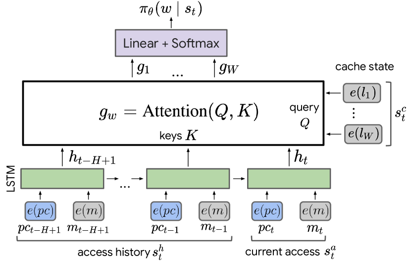
Figure 1: The analyzed caching model [Liu et al., 2020].

The Caching Model Figure 1 shows an overview of the model’s architecture. The model has an LSTM layer, an attention layer, followed by a final fully connected layer. The model’s input is a time series of cache accesses. Each access is encoded using an embedding of the program counter $e(p)$ and the memory address $e(m)$. To make an eviction decision, the model calculates an eviction score. First, the cached address embedding is used as attention key and the LSTM’s hidden state as attention query and value. Based on the attention output, a fully connected layer then computes the score. The item with the highest score is evicted. The model is trained using imitation learning to replicate the optimal policy during training, based on memory traces from the SPEC2006 benchmarks [Henning, 2006] The work trains a separate model for each execution trace (see [Liu et al., 2020] for details).

3 Analyzing the Caching Model

Explaining and characterizing the model’s abstraction level can be done in different ways. As a start, we analyze the memory address trace and the model’s performance statistics.

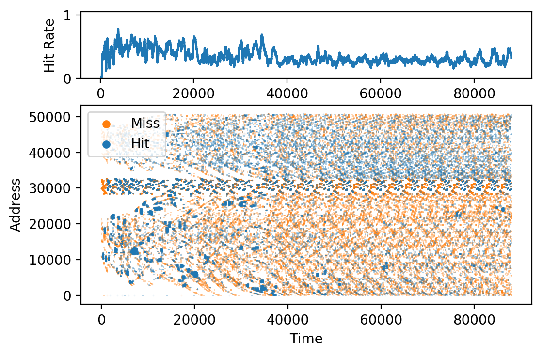
(a) astar

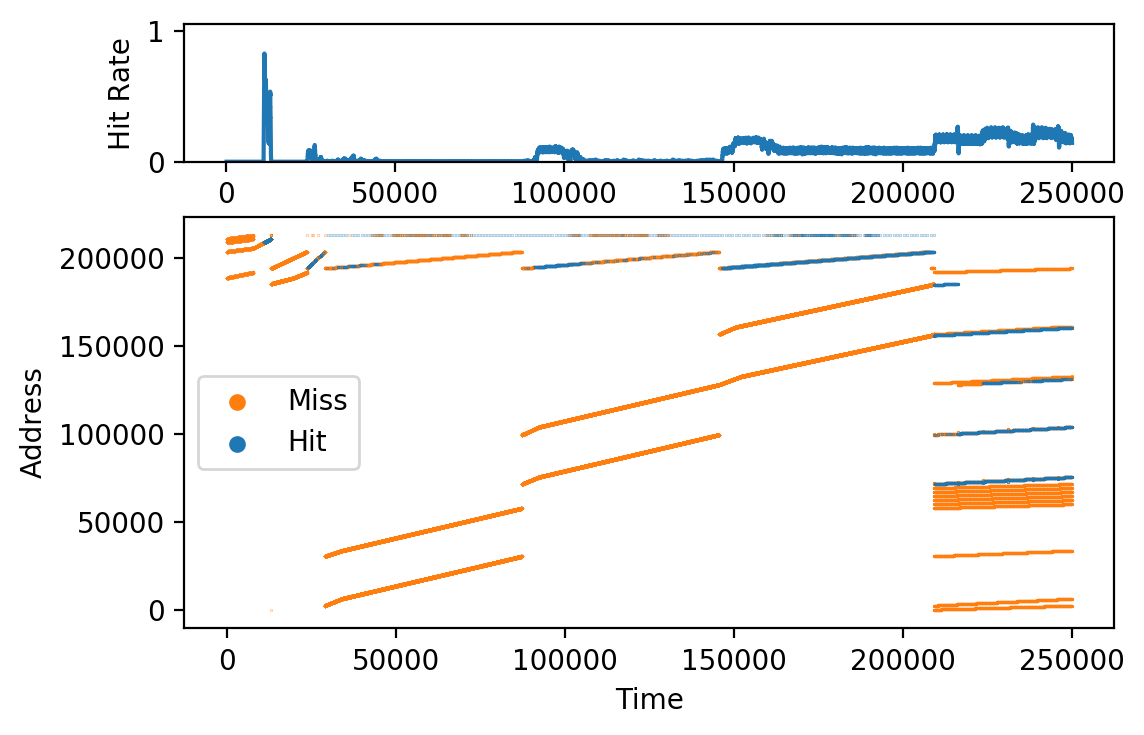
(b) bwaves

(c) bzip

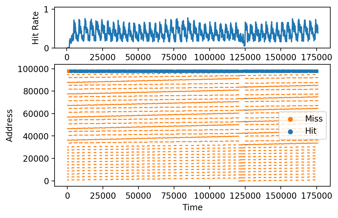
(d) cactusadm

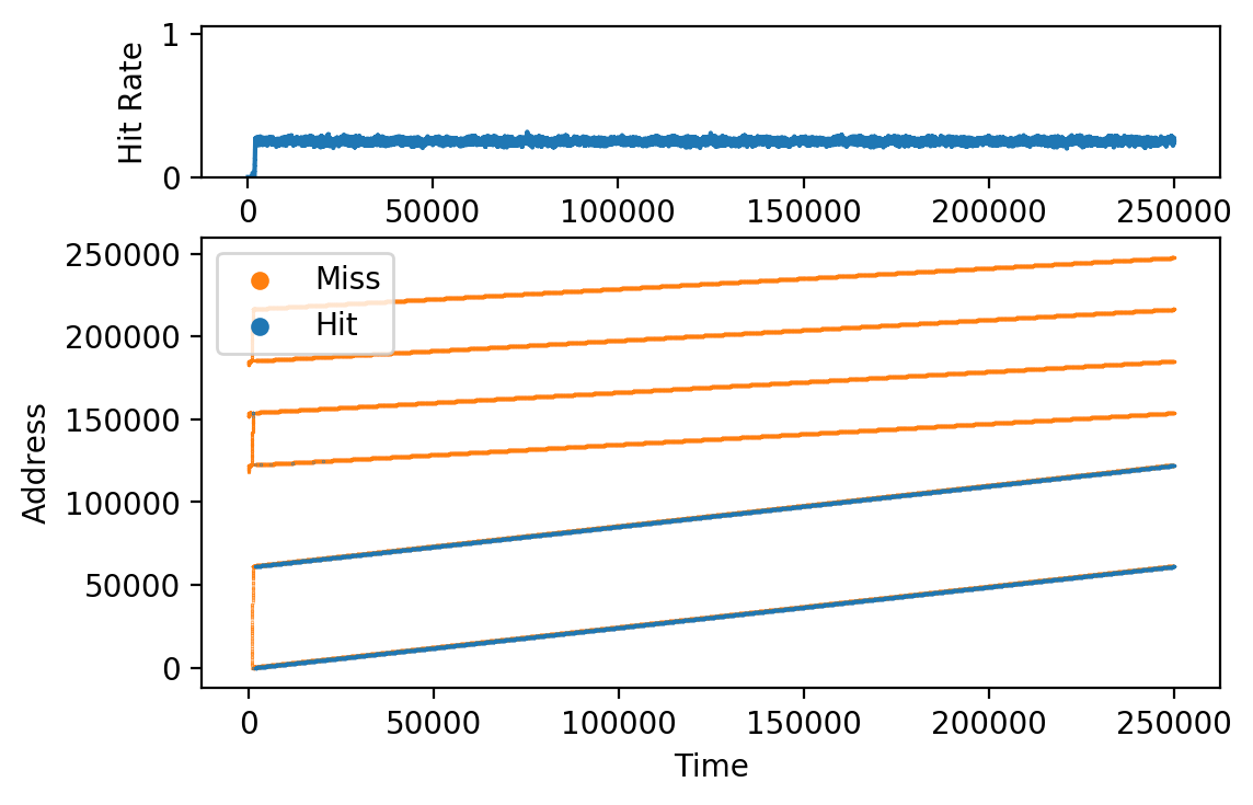
(e) gems

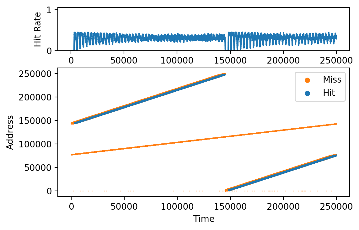
(f) lbm

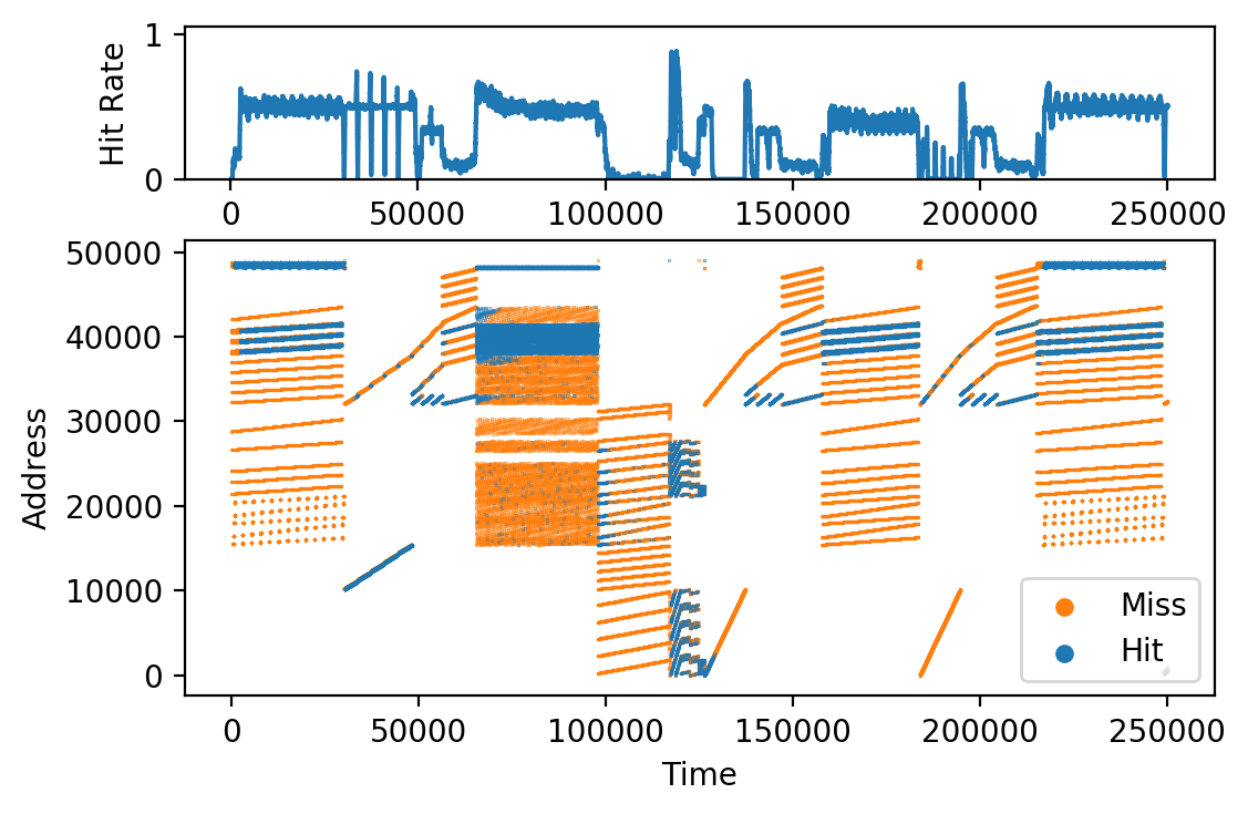
(g) leslie3d

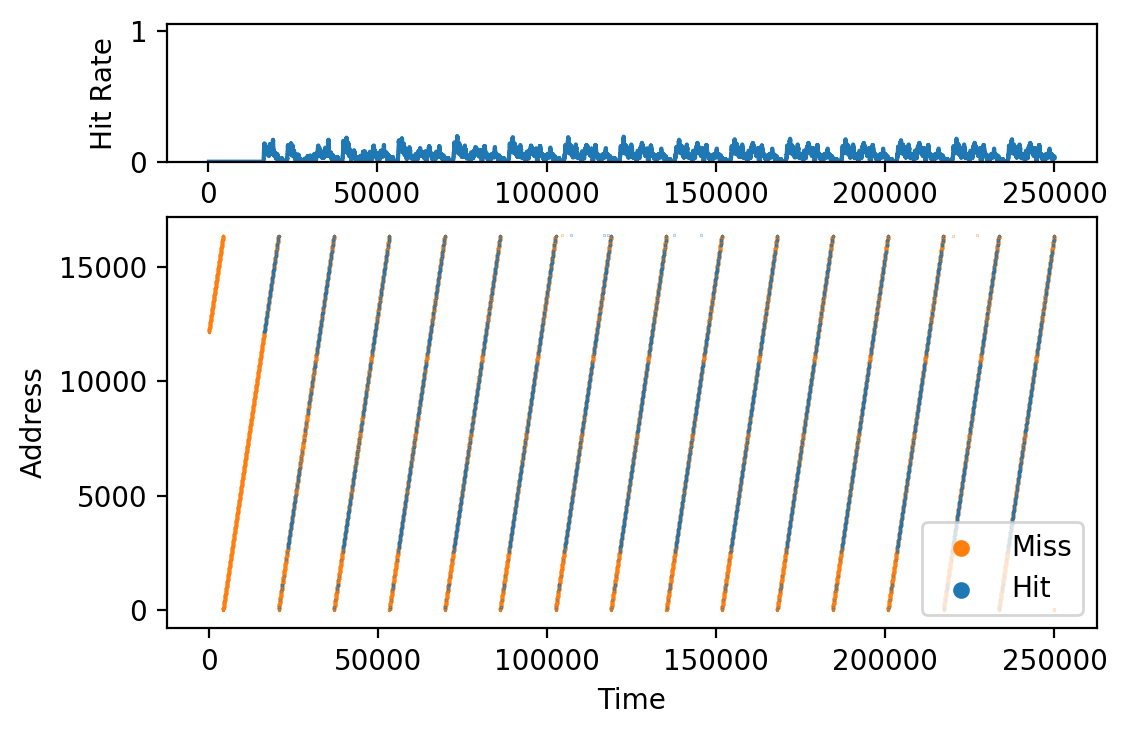
(h) libq

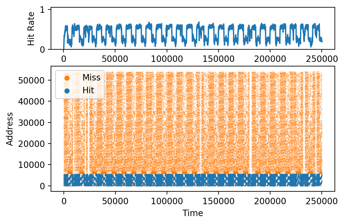
(i) mcf

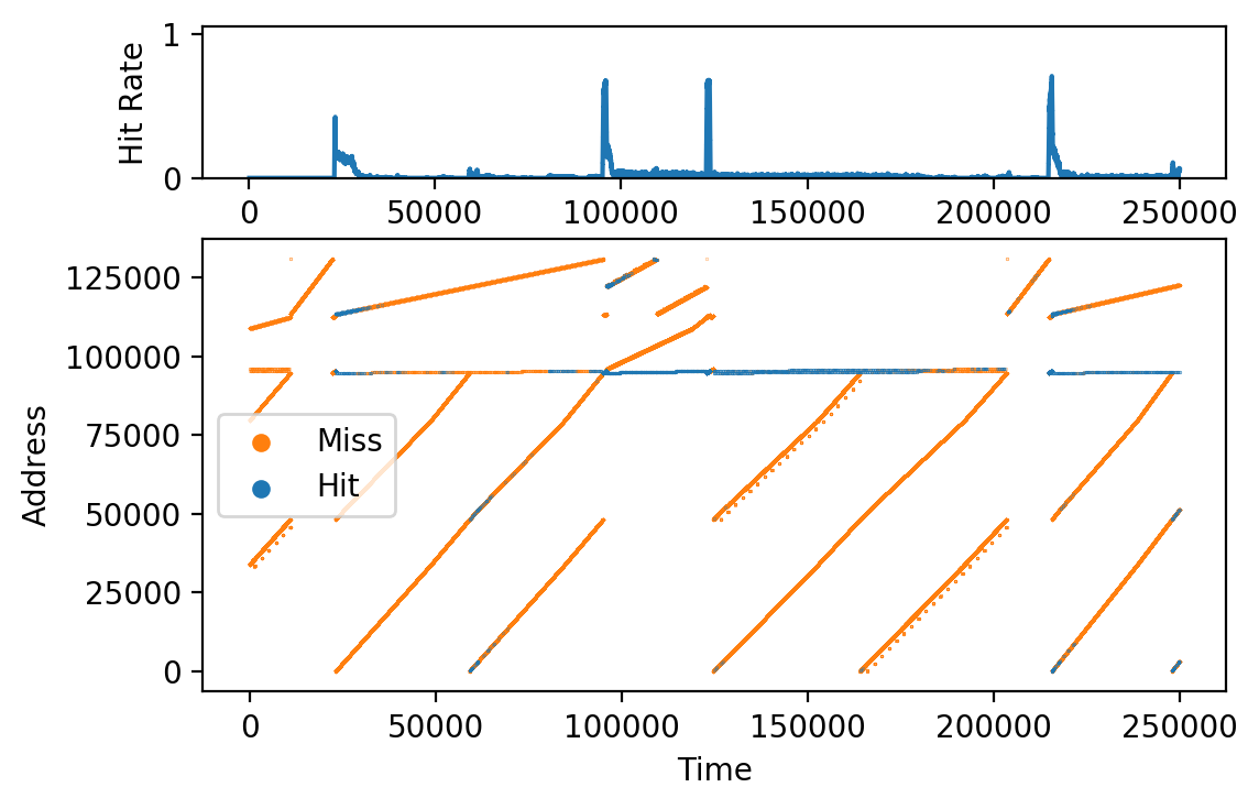
(j) milc

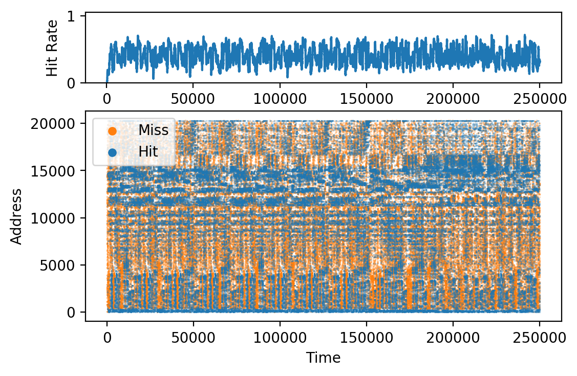
(k) omnetpp

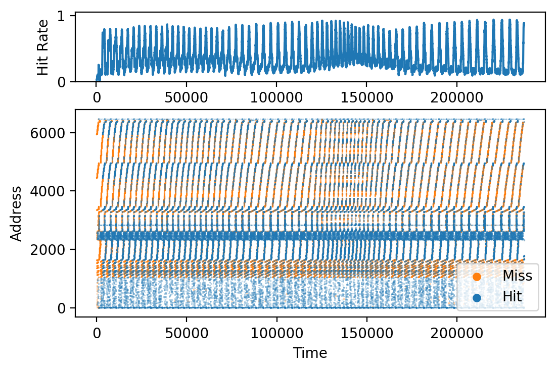
(l) sphinx3

(m) xalanc

Figure 6: Cache hits and misses of the learned policy

Visualising the Execution and Performance Statistics For each time step, we plot the accessed address and whether it was a hit or a miss. The hit rate can be visualised using a rolling mean (see Figure 2 and Appendix Figure 6). Inspecting these visual diagrams provides a first impression about the behaviour of the model on the different traces. For example, the hit rate is almost constant for lbm and gems. The executions for bzip and leslie3d are separated into repeating phases. High frequency oscillations happen on cactusadm, sphinx3, and mcf. bwaves, libq, milc are difficult to cache and their the hit rates are zero most of the time.

Table 1: (H1) Cache hit rates for different policies. Bélády is the optimal policy. For the Address & Phase baseline, we used a lookup-table per address and phase and evict an address based on its frequency. Entries where the baseline performs close to the model are shown in bold.

Policies	astar	bwaves	bzip	cact.	gems	lbm	leslie3d	libq	mcf	milc	omne.	sphinx3	xalanc
Belady	43.5	8.7	78.4	38.8	26.5	31.3	31.9	5.8	46.8	2.4	45.1	38.2	33.3
Model	34.3	7.8	64.5	38.7	26.2	30.8	31.8	5.1	41.1	2.1	40.3	36.6	30.4
Address & Phase	27.7	1.3	62.1	35.1	6.9	0.1	21.0	0.0	37.9	0.4	28.2	34.4	22.4

Information encoded in the address embedding In a further analysis, we look at possible limitations of the network architecture. Here, the address embedding stands out as it might limit generalization. Each memory address is assigned a unique embedding vector. However, the memory layout can be very different between two runs of the identical program (modern OSs employ address space randomization). We would therefore like to test which information is encoded in the memory address embedding.

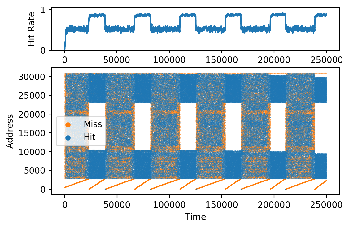
Figure 2: Hits and misses. Per time step, we plot the access memory address and if it was a hit or misses. on the top, the hit rate of the model is shown.

Experiment: We apply Principal Component Analysis (PCA) on the address embeddings. The first several Principal Components (PCs) account for the most variance and are thus a good proxy for the encoded information in the embedding.

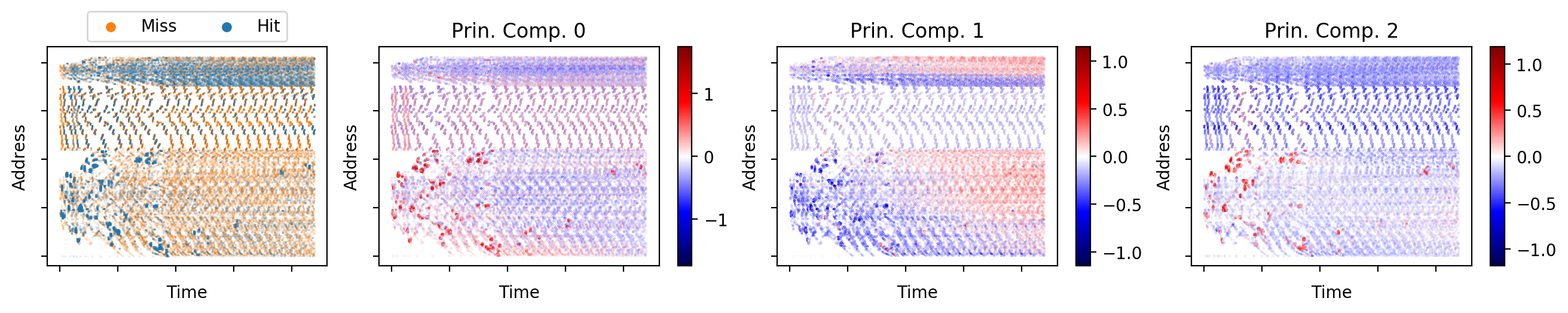
(a) astar

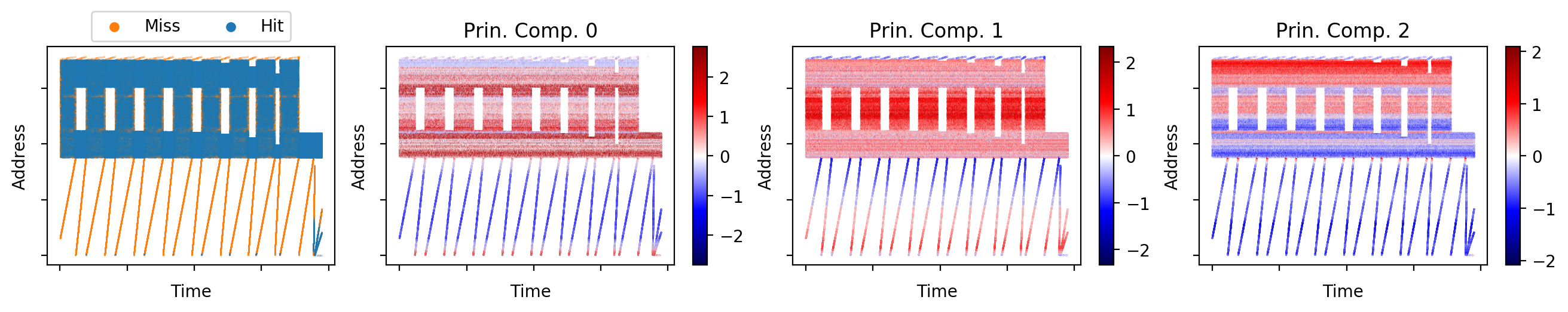
(b) bzip

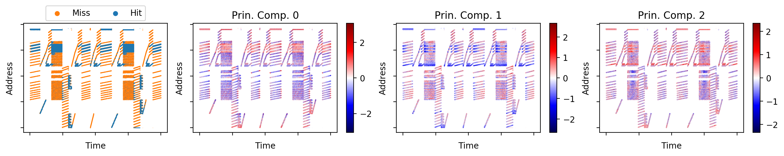
(c) leslie3d

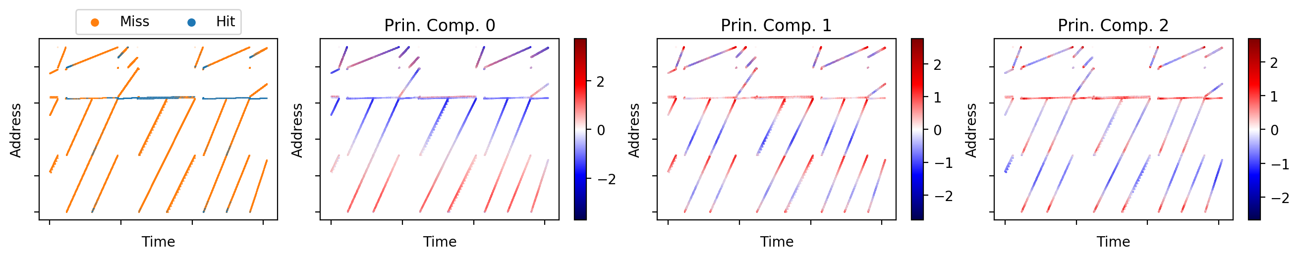
(d) milc

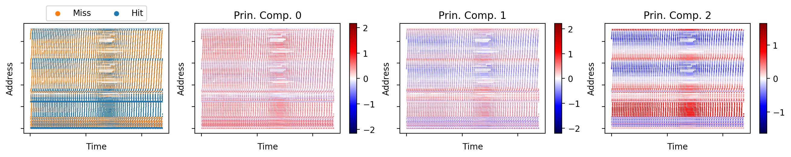
(e) sphinx3

Figure 7: PCA of address embeddings. First, the hit rates are shown, then the top-3 principal components. The principal components (PC) correlate with the hits and misses.

Result: In Figure 7, we display the hits and misses along with the first three principal components of the address embeddings. We see that trace-specific features are encoded in the address embedding. For example, PC2 (principal component 2) of bzip changes in tandem with distinct sequential access patterns in the lower address space. The results from the other benchmarks also support the claim that the address embeddings encode trace-specific features. For example, for astar the PC0 and PC2 seem to encode addresses that lead to cache hits. The trace-specific embedding means that a model cannot generalize to new traces if the memory is allocated at a different location.

A simple baseline for caching based on simple statistics As the address embedding encodes trace-specific information, a natural explanation of the model’s behavior would be that it memorizes which addresses to cache based on the current execution state. To test this hypothesis, we construct a policy based on a simple lookup table and compare the model’s performance to it. We also include the optimal Bélády policy as reference. If a lookup policy performs similarly to the model, we would conclude that no high-level reasoning is needed.

Experiment: We construct a simple caching policy based on how often each address occurs per ”phase”-type. A phase is a reoccurring pattern within the execution. We isolate these phases from the trace using a hierarchical clustering based on statistics of the program counter and reuse distance (i.e., the time until an address is used again; see Appendix A for details). The lookup table policy always evicts the least-used addresses given the current phase. We then compare the hit rates between the simple lookup table, the Bélády’s policy, and the model.

Result: For most of the benchmarks, the simple policy using the frequency of access alone is insufficient to achieve similar performance to the model (see Table 1). Therefore, the model must use a representation beyond these simple statistics.

Inter-phase variability As we invalidated the lookup table hypothesis, we can reasonably conclude that the model is capable of more complex reasoning than a simple lookup table of frequency statistics and phases. However, what is the specific difference? Has the model a finer resolution than phases? Which additional information does the model encode that is not included in simple statistics?

Experiment: To answer these questions, we inspect the model’s internal state by applying PCA to the LSTM’s hidden state. We use the hidden state as it is central to the model’s behavior. Any variation in model output is grounded either in the embeddings or the hidden state, as they represent the attention queries, keys, and values. PCA is the natural choice to describe the main directions of variance and can be used without any labels. Generally, the lack of labels is also the largest drawback of PCA, as the PCs do not have to correspond to semantically meaningful concepts. By looking at the top-5 principal components, we can understand whether the model’s activation varies within a phase or not.

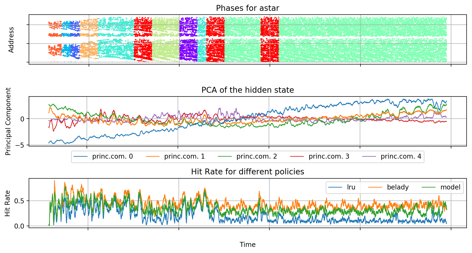
(a) astar

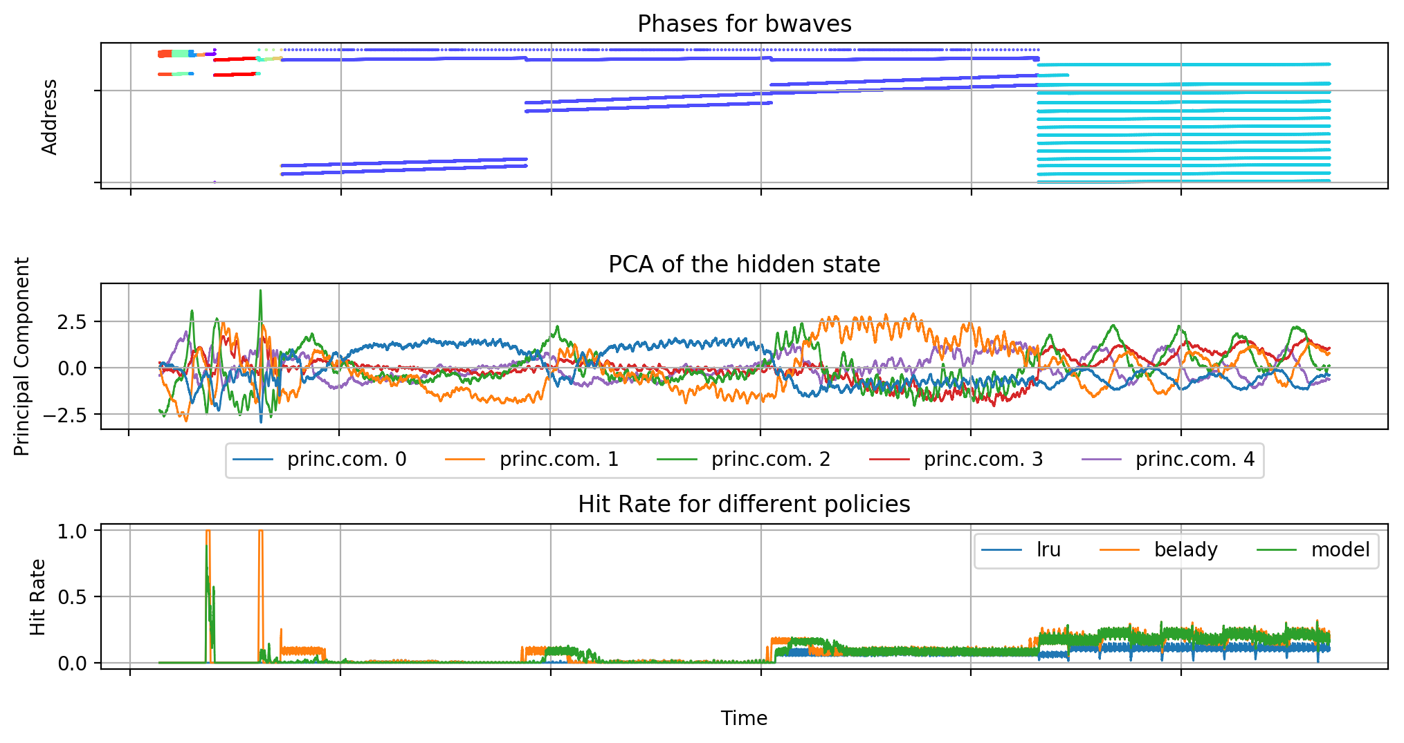
(b) bwaves

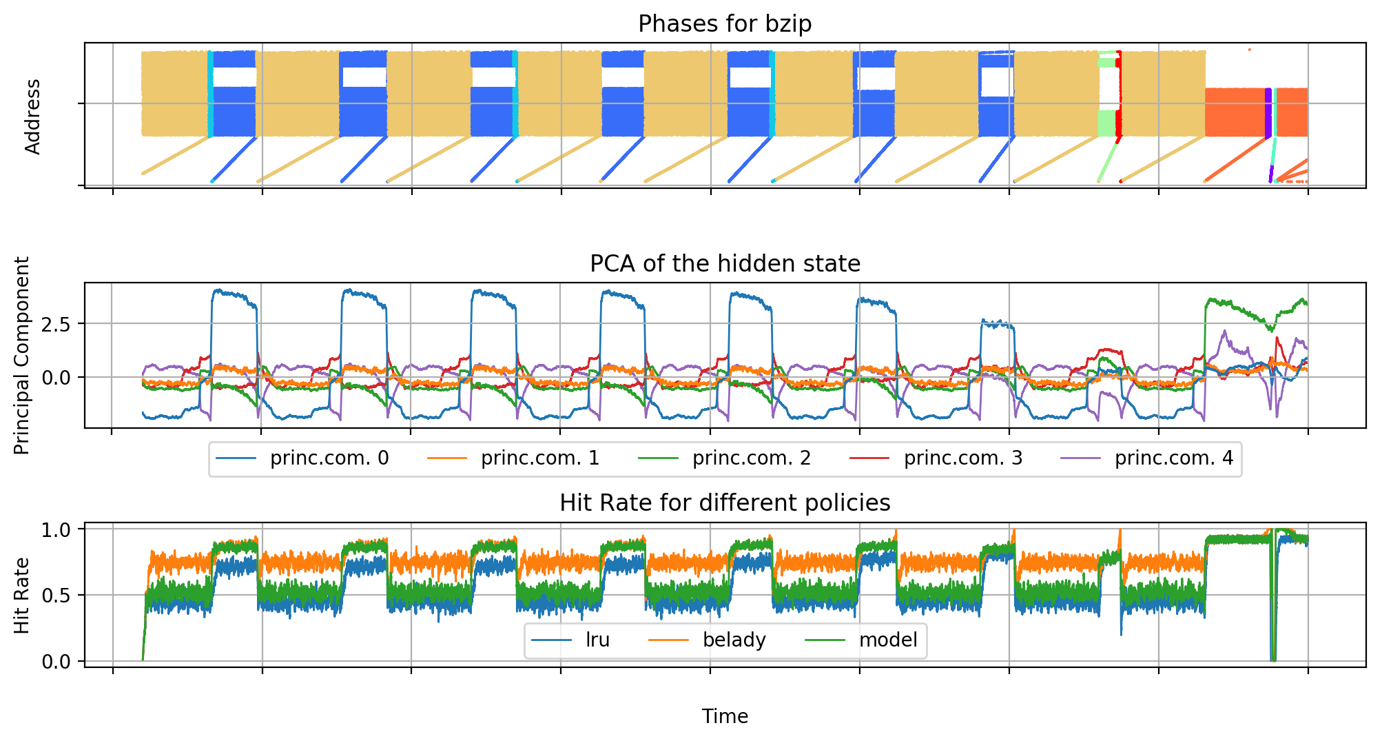
(c) bzip

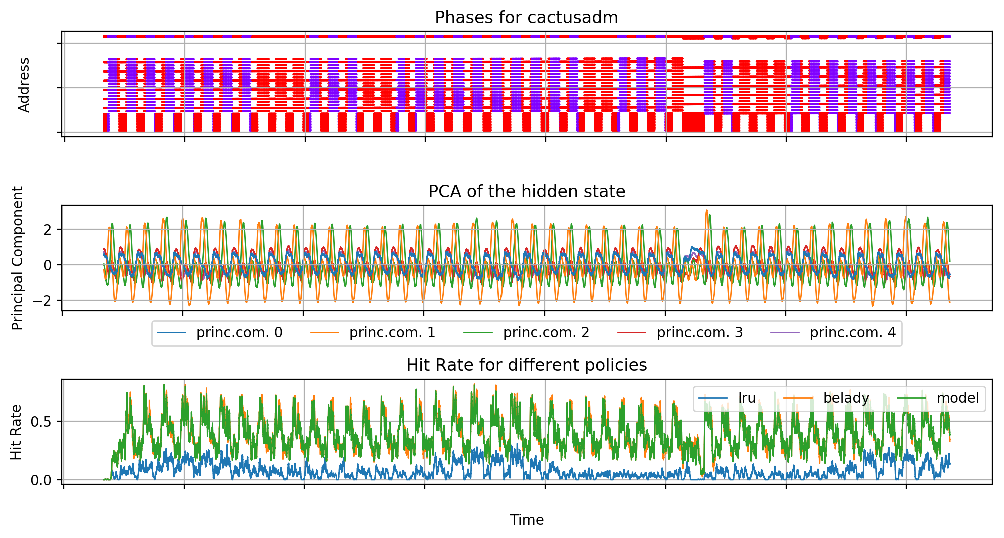
(d) cactusadm

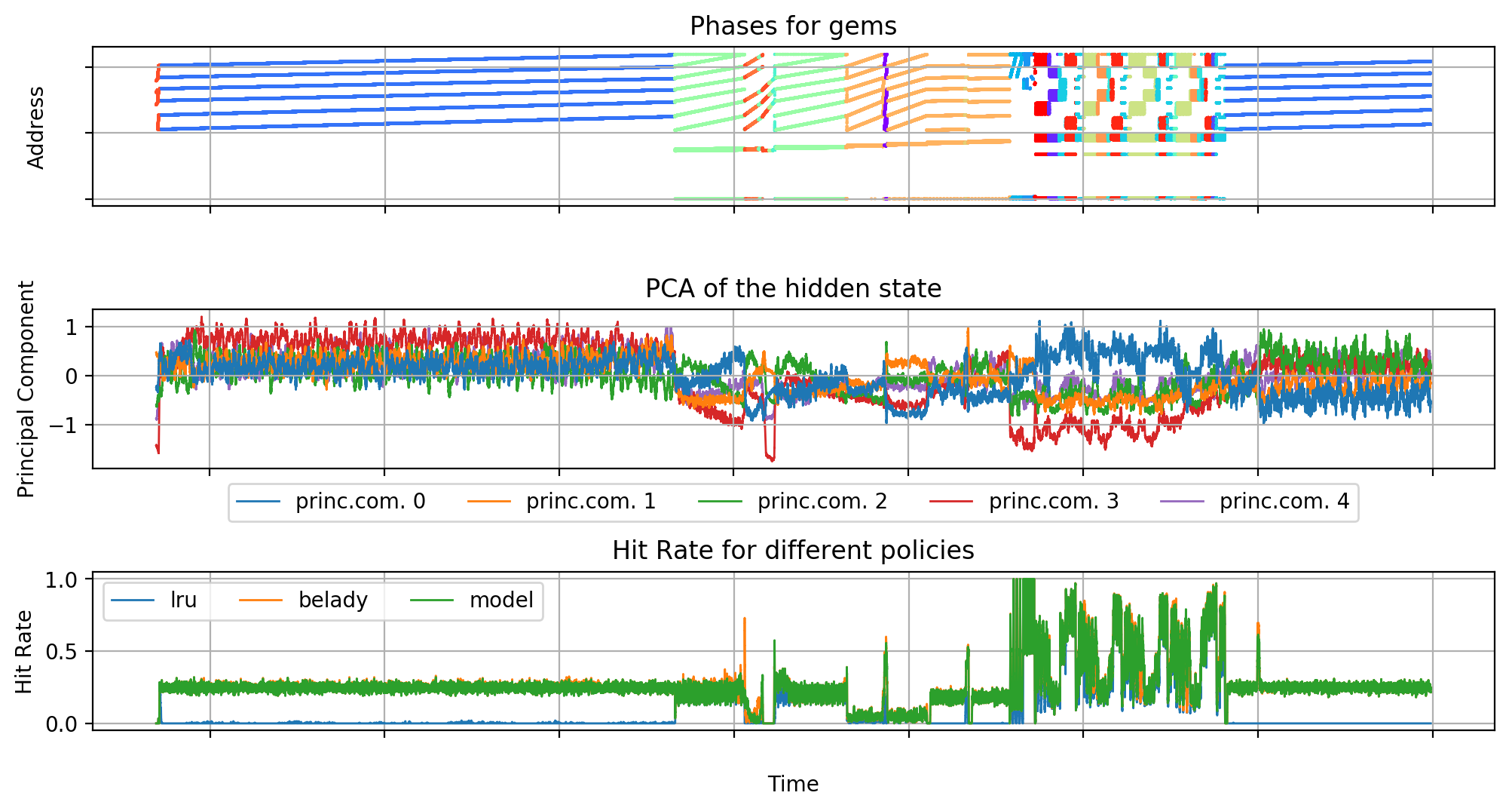
(e) gems

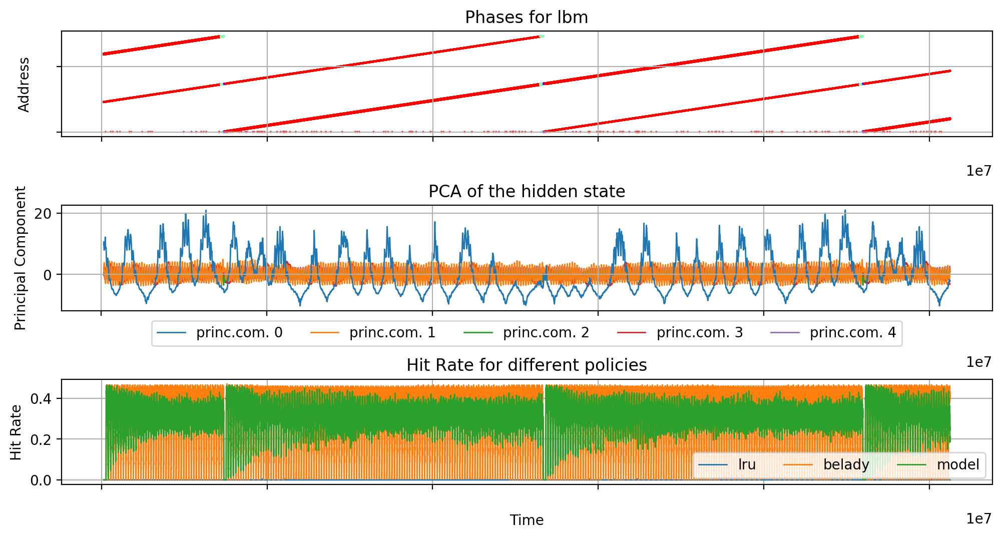
(f) lbm

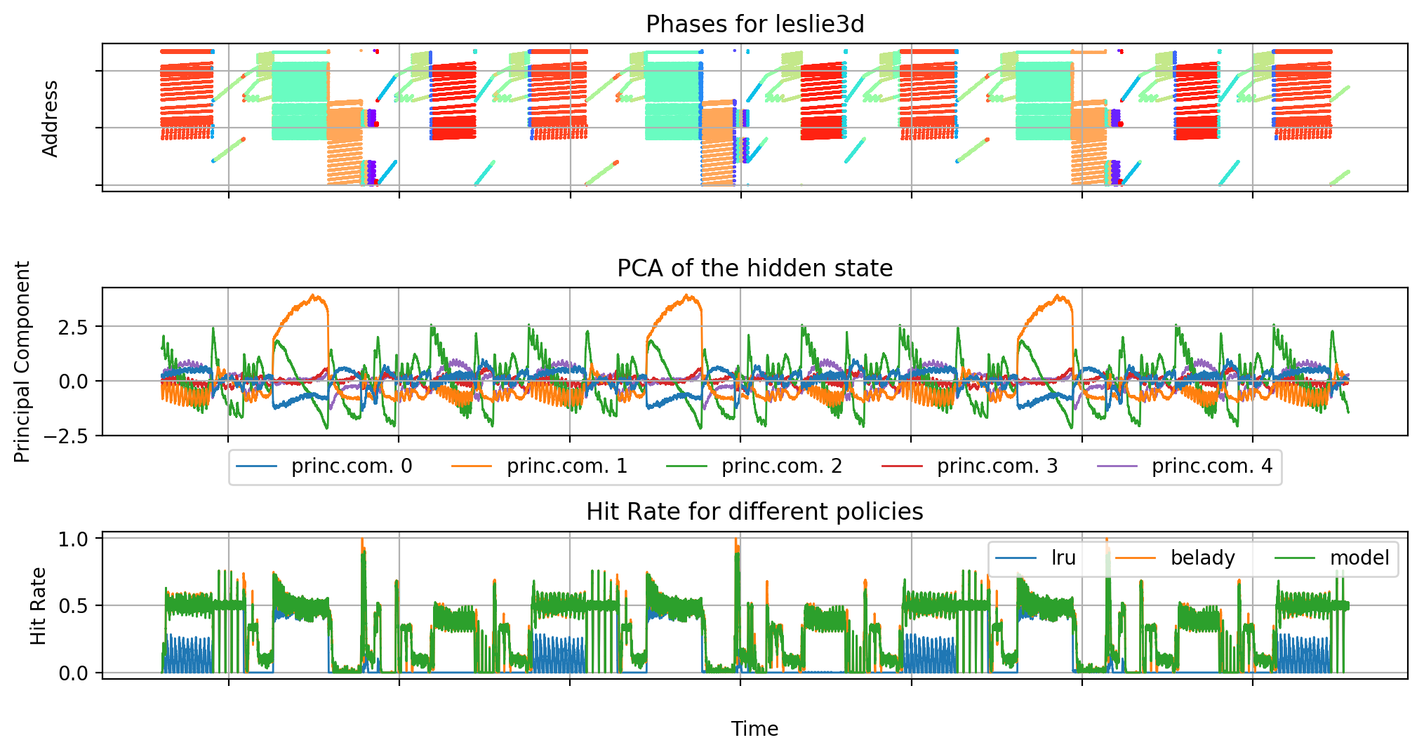
(g) leslie3d

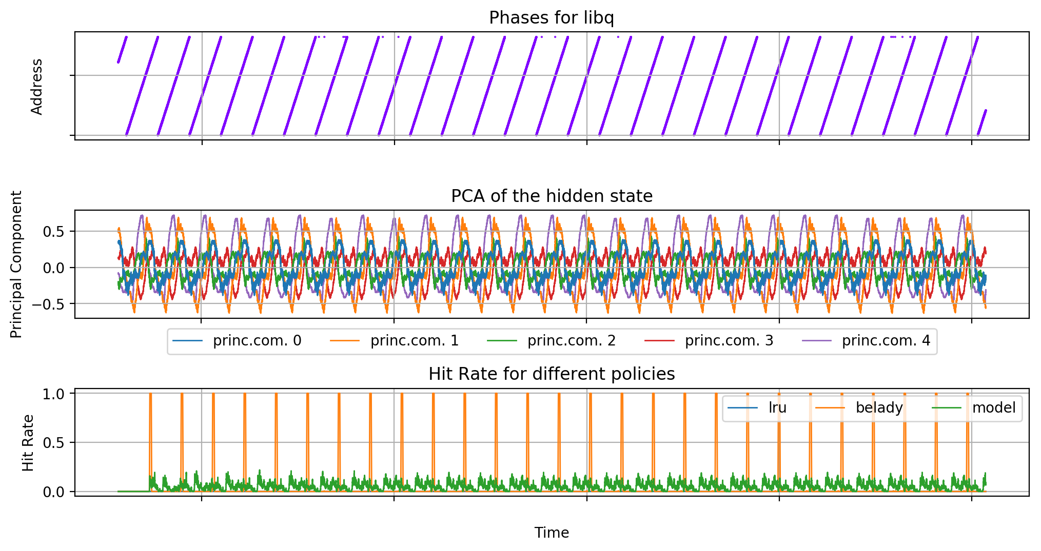
(h) libq

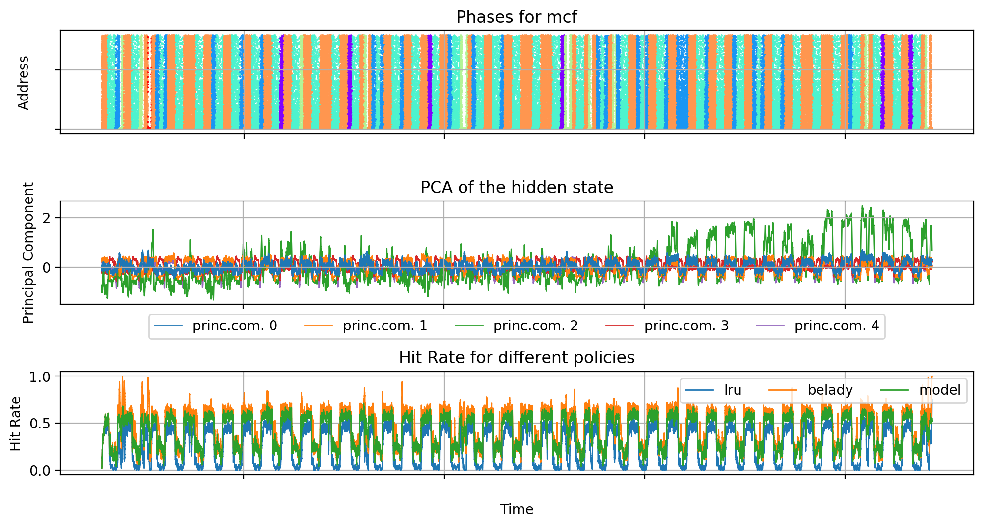
(i) mcf

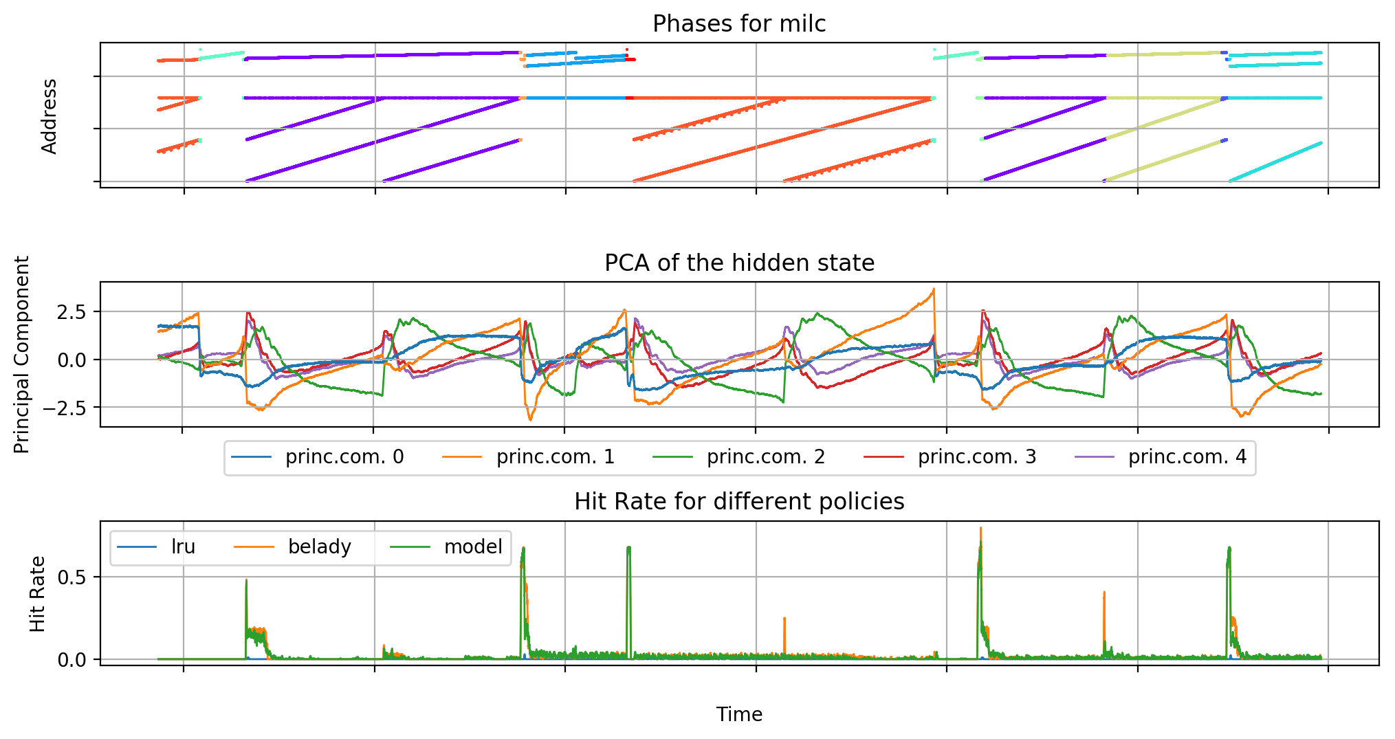
(j) milc

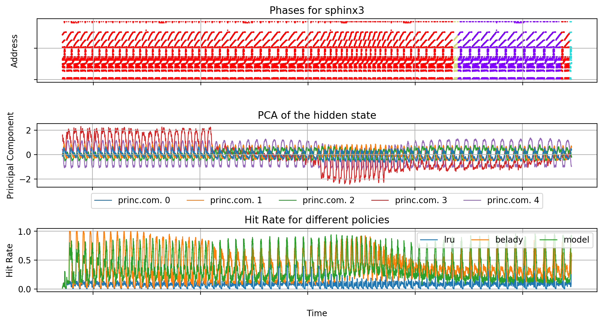
(k) sphinx3

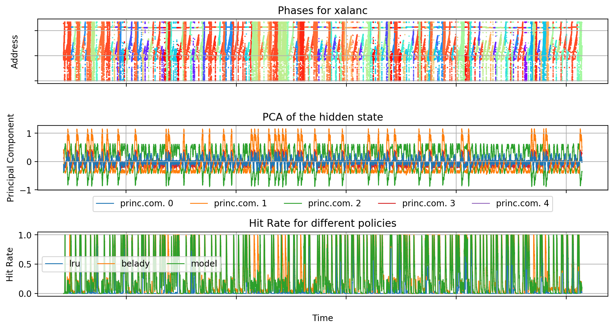
(l) xalanc

Figure 8: On the top, discovered phases. In the middle, the PCA of the hidden state. On the bottom, the hit rates of the learned policy, LRU and Bélády.

Result: As seen in Figure 3(a), the principal components change within each phase in bzip. While the first principal component is strongly correlated with the two main phases (r=0.89 and -0.83), other principal components vary within each phase. Some of these changes seem to be correlated with semantically meaningful changes. For example, a jump in four out of five top principal components just before the end of the red phase in Figure 3(a) may indicate that the jump encodes the end of the red phase – a reasonable behaviour for models since some addresses are not needed in the next phase. On other programs, we can see similar behaviors. For example, leslie3d also exhibits strong inter-phase variations (see PC1 in Figure 8(g)). These results indicate that the hidden state of the model has no simple interpretation and varies within each phase. This rules out simple explanations that would allow an engineer to reason about the model in terms of phases and ignore individual accesses.

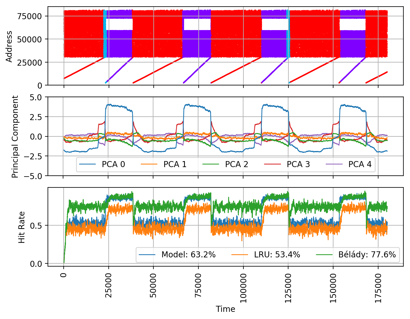
(a) Original bzip memory trace

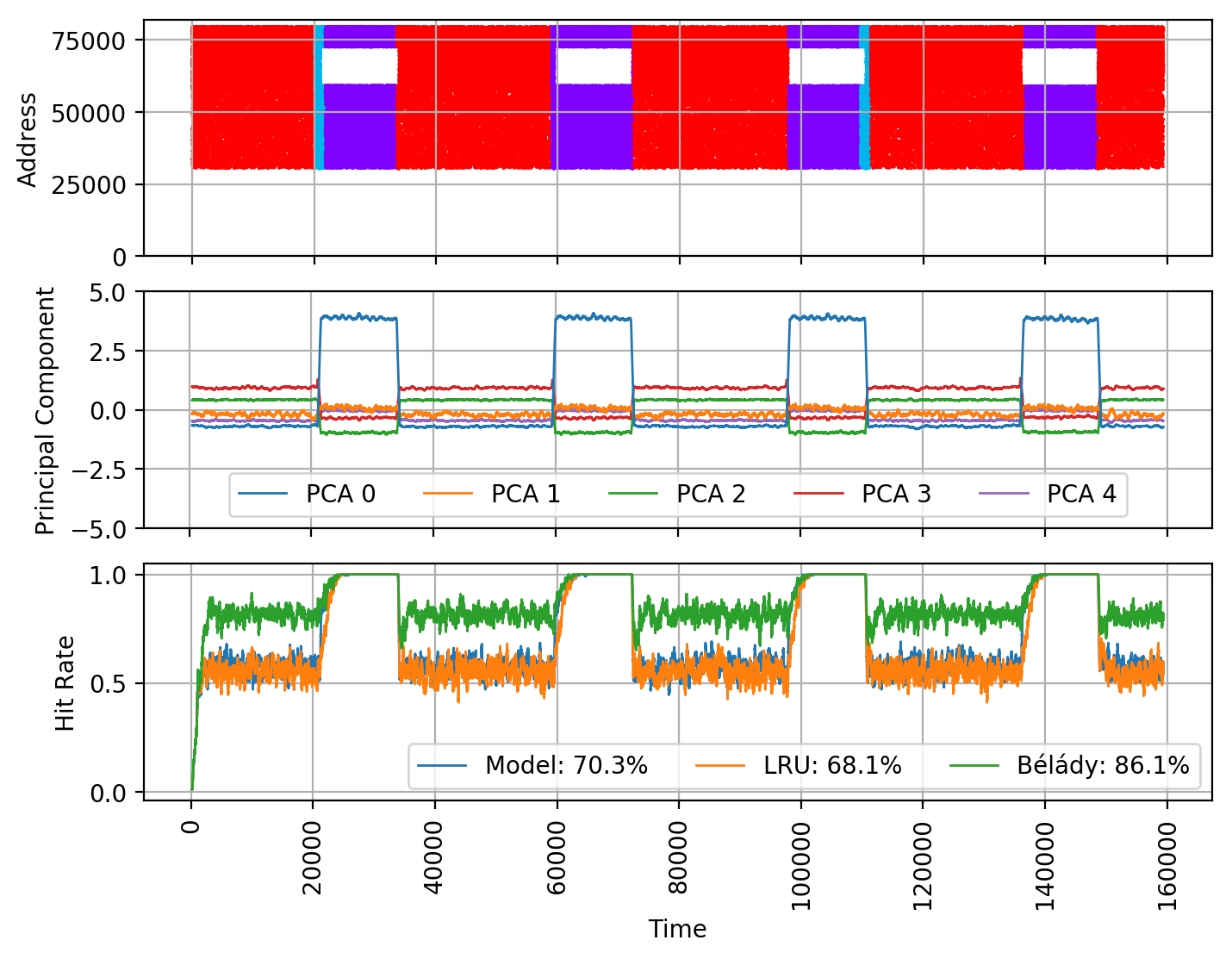
(b) Lower streams removed

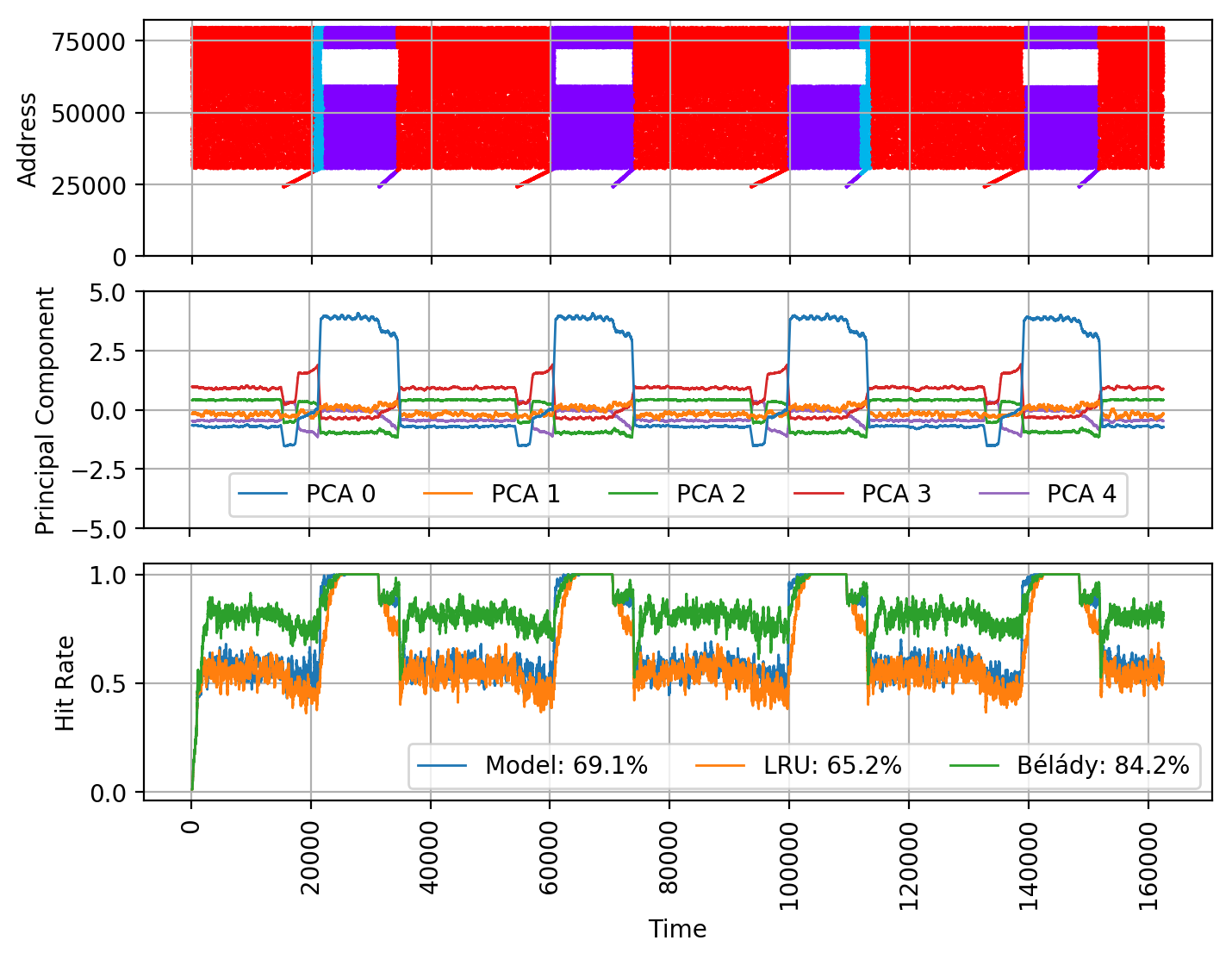
(c) End part of lower stream included

Figure 3: On top, the memory trace of bzip with sequential access patterns (streams) at the lower end of the address space. In the middle, the top-5 principal components. On the bottom, the hit rates of the model, LRU and Bélády. (a) the original trace. A distinct jump in PCA componenents can be seen at at end of the red phase. (b) when the streams are removed, all variability with a phase disappears – showing that the streams are responsible for encoding differences within a phase. (c) Including only the end part of the lower stream still shows the distinct jump – suggesting that the model’s behavior depends on specific memory addresses.

Modifications of Streams The previous experiment suggests that the model encodes phases and also variations within a phase. This calls to analyze which patterns cause the variations. In particular, we test what happens if a stream (a sequential access pattern) is removed. A stream corresponds to a linearly increasing memory addresses that are accessed in sequence, e.g by looping over an array. An example can be seen in the lower lines in Figure 2. Both phases and streams are more abstract, or high-level, concepts than raw individual memory addresses. The question is: Is the model aware of these concepts?

Experiment: We remove streams and see how the model behavior changes. If the model encodes streams, we would expect to see changes in the hidden activations.

Result (bzip): Figure 3(b) shows the results of removing the streams on bzip. Removing the streams erases almost all variability in principal components. Before erasing, PC0, PC2, PC3, PC4 make a distinctive jump before the end of the red phase (see Figure 3(a)). Once the streams are erased, the jumps are gone. Therefore, the model relies on the streams to encode the near ending of the phase.

Result (milc): The milc program has a phase with 4 different streams (orange in Figure 5(a)). The principal component 2 (green) switch its sign when the two smaller orange streams switch. One could assume that as PC2 correlates with the streams it also encodes information about them. However, this is not the case. When the streams are removed PC2 bearly changes (see Figure 5(b)). In contrast, if the larger stream is removed, than PC2 does change (see Figure 5(c)).

4 Conclusion

We have provided a first set of analyses towards the interpretability of a caching model. Specifically, we examined the level of abstraction at which the caching model operates. We learned that while the address embedding memorizes trace-specific information, the model learns higher-level behaviour and can represent different phases and their transitions. It turned out that the concept of streams is particular relevant for encoding these transitions. The conducted analysis shed some light into the typical behaviour of the model and the benefit of using concept-based explanations in caching models. Nevertheless, further analysis is required to close the gap between the way humans reason about programs and the caching model’s low-level inputs. An interesting research direction for future work would be to create a model that combines the two worlds of low-level machine behavior and high-level information, e.g., memory addresses or machine code with a summary of the source code.

Appendix A Extraction of Program Phases

Many execution traces show recurring patterns. Examples include bzip, which has two distinct phases, or leslie3d. (see Figure 4). These phases typically correspond to different parts of code in a program that execute one after another, such as loading an input file and performing an operation on it.

Phase Finding The goal of the phase finding algorithm is to extract highly similar phases using the input features of the trace. Existing methods [Shen et al., 2018, Sherwood et al., 2002] find phases using k-means. We decided against using them. Besides having to select the number of clusters, k-means also has the disadvantage that a data point can be far away from the cluster center as long as it is the closest center, which can lead to very high variability within a phase. However, we require a phases to be very uniform. If we characterize the model using phases, we do not want to have to account for inter-phase variability.

The phase finding algorithm performs clustering based on Reuse Distance Vectors [Shen et al., 2018]. Reuse Distance Vectors compute a histogram over the distance between accesses to the same address. The reuse distance is closely related to cacheability. As an additional feature, we use the histograms of the delta of program counters. The delta in program counters captures program execution at a mechanical level (e.g., 1 means that the program stepped to the next instruction, a short positive jump indicates a branch, and a long jump in any direction indicates a function call). In Figure 4, we show the two histograms used as features to the phase finding.

We rely on the assumption that a trace will remain in each phase for a meaningful amount of time. We therefore first split a trace into small slices and then merge neighbouring slices if they are highly similar. As metric, we use the L1-distance between the histograms of the reuse distance and the deltas of the program counters computed per slice. Once no more neighbouring slices are merged together, we find globally similar phases using the same metric. We select the hyperparameters conservatively to ensure only highly similar execution parts are merged together.

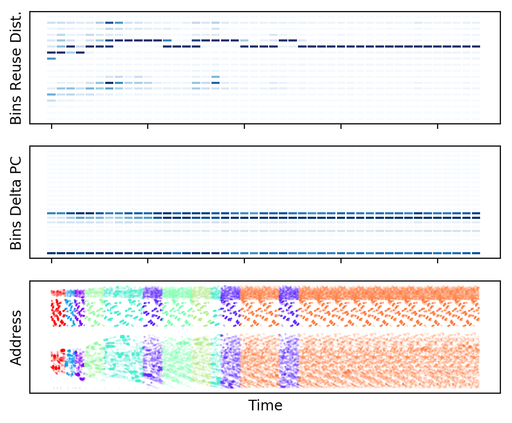
(a) astar

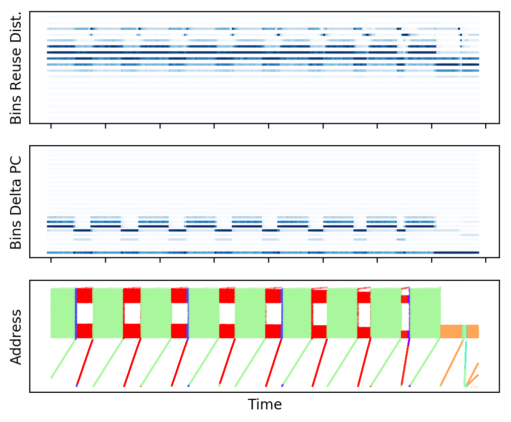
(b) bzip

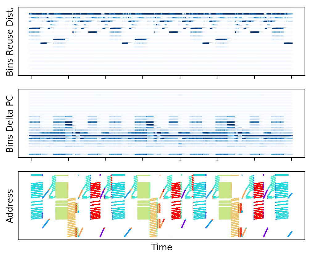
(c) leslie3d

Figure 4: Features used for finding the phases, and the phases themselves. On top, the histograms of the Reuse Distance. Below, the histogram of the delta program counter. On the bottom, the discovered phases.

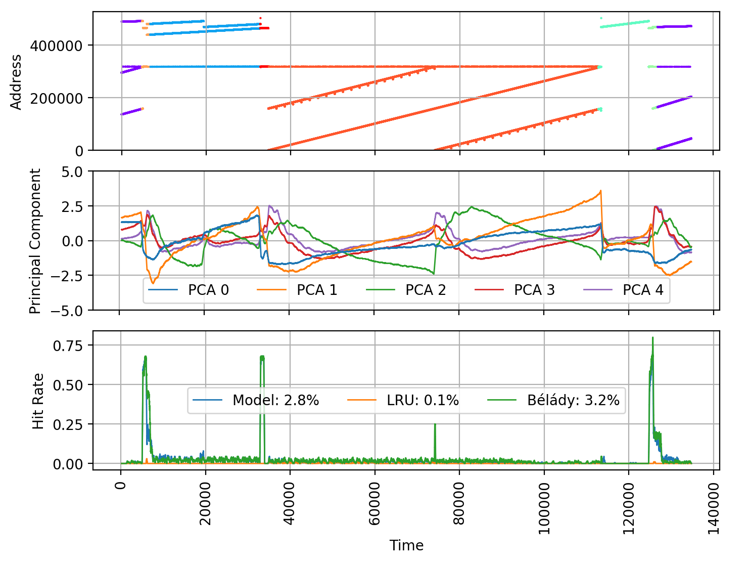
(a) Original milc trace

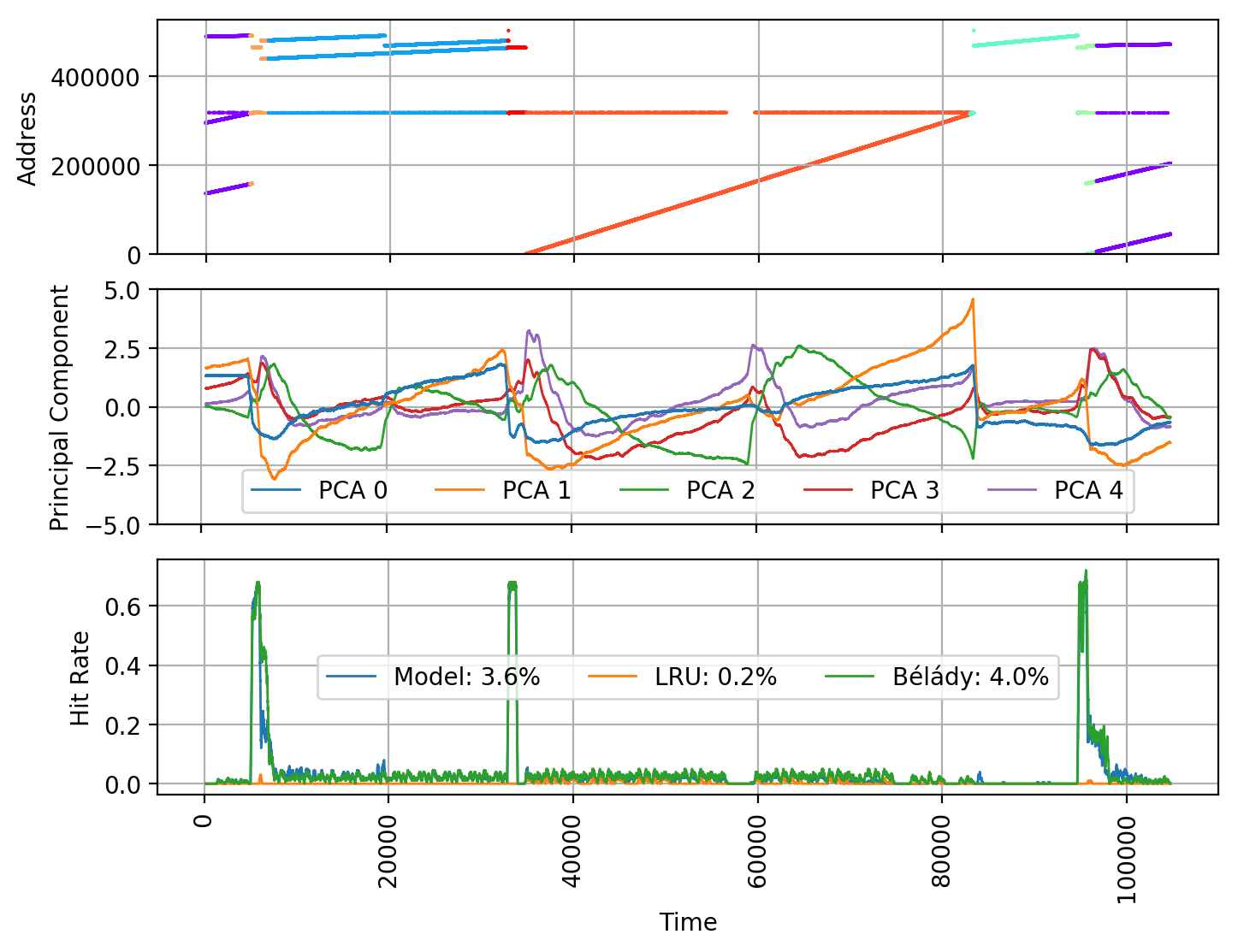
(b) Milc after removing two streams

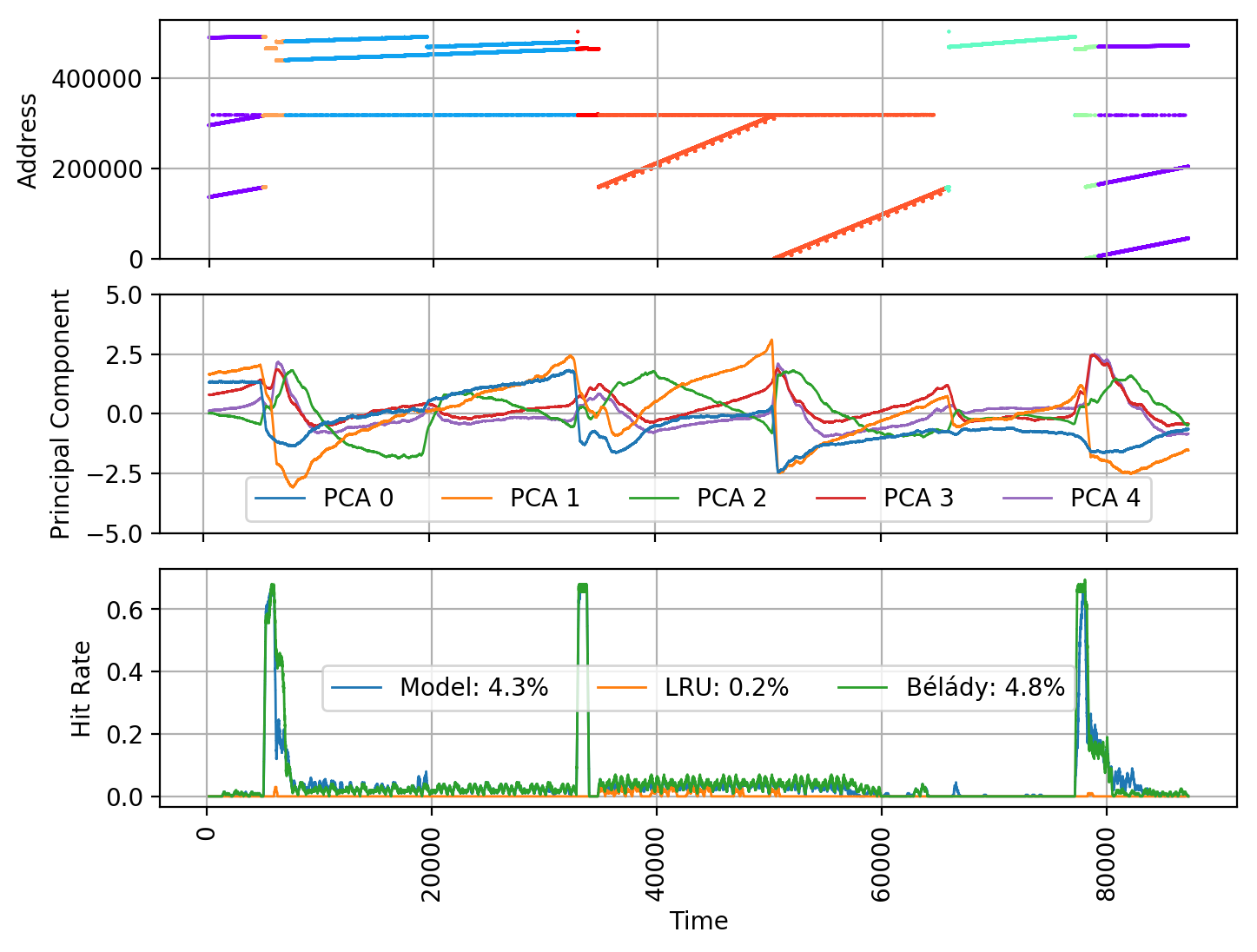
(c) Milc after removing long stream

Figure 5: The milc program has a phase with 4 different streams: in orange (a). The sign switch of the principal component 2 (green) co-occurs with the switch of the two smaller streams. However, removing them in (b) does not change the flip. Indeed, the PCs’ magnitude barely changed (mean abs. difference: 0.075). When the long stream is deleted (c), the green PCA2 changes to show less variability (mean abs. diff: 0.571). Additionally, the orange PCA1 switches sign. As the streams access the same memory, their differences has to come from the program counters. And indeed, each stream can be traced back to different program counters accessing the same memory.

References

- Bélády [1966] L. A. Bélády. A study of replacement algorithms for a virtual-storage computer. IBM Systems Journal, 5(2):78–101, 1966. doi: 10.1147/sj.52.0078.
- Cen et al. [2020] L. Cen, R. Marcus, H. Mao, J. Gottschlich, M. Alizadeh, and T. Kraska. Learned garbage collection. In Proceedings of the 4th ACM SIGPLAN International Workshop on Machine Learning and Programming Languages, pages 38––44, New York, NY, USA, 2020. Association for Computing Machinery.
- Cohn and Singh [1997] D. A. Cohn and S. P. Singh. Predicting lifetimes in dynamically allocated memory. In M. C. Mozer, M. I. Jordan, and T. Petsche, editors, Advances in Neural Information Processing Systems 9, pages 939–945. MIT Press, 1997.
- Hashemi et al. [2018] M. Hashemi, K. Swersky, J. Smith, G. Ayers, H. Litz, J. Chang, C. Kozyrakis, and P. Ranganathan. Learning memory access patterns. In Proceedings of the 35th International Conference on Machine Learning, volume 80 of Proceedings of Machine Learning Research, pages 1919–1928, Stockholmsmässan, Stockholm Sweden, 10–15 Jul 2018. PMLR.
- Henning [2006] J. L. Henning. Spec cpu2006 benchmark descriptions. SIGARCH Comput. Archit. News, 34(4):1–17, Sept. 2006. ISSN 0163-5964. doi: 10.1145/1186736.1186737. URL https://doi.org/10.1145/1186736.1186737.
- Liu et al. [2020] E. Liu, M. Hashemi, K. Swersky, P. Ranganathan, and J. Ahn. An imitation learning approach for cache replacement. In International Conference on Machine Learning, pages 6237–6247. PMLR, 2020.
- Maas [2020] M. Maas. A taxonomy of ml for systems problems. IEEE Micro, 40(5):8–16, 2020.
- Maas et al. [2020] M. Maas, D. G. Andersen, M. Isard, M. M. Javanmard, K. S. McKinley, and C. Raffel. Learning-based memory allocation for c++ server workloads. In Proceedings of the Twenty-Fifth International Conference on Architectural Support for Programming Languages and Operating Systems, ASPLOS ’20, pages 541–556, New York, NY, USA, 2020. Association for Computing Machinery.
- Mao et al. [2019] H. Mao, M. Schwarzkopf, S. B. Venkatakrishnan, Z. Meng, and M. Alizadeh. Learning scheduling algorithms for data processing clusters. In Proceedings of the ACM Special Interest Group on Data Communication, SIGCOMM ’19, pages 270––288, New York, NY, USA, 2019. Association for Computing Machinery.
- Shen et al. [2018] S. Shen, M. Ling, Y. Zhang, and L. Shi. Detecting the phase behavior on cache performance using the reuse distance vectors. Journal of Systems Architecture, 90:85 – 93, 2018. ISSN 1383-7621. doi: https://doi.org/10.1016/j.sysarc.2018.09.001. URL http://www.sciencedirect.com/science/article/pii/S1383762118302248.
- Sherwood et al. [2002] T. Sherwood, E. Perelman, G. Hamerly, and B. Calder. Automatically characterizing large scale program behavior. In Proceedings of the 10th International Conference on Architectural Support for Programming Languages and Operating Systems, ASPLOS X, page 45–57, New York, NY, USA, 2002. Association for Computing Machinery. ISBN 1581135742. doi: 10.1145/605397.605403. URL https://doi.org/10.1145/605397.605403.
- Song et al. [2020] Z. Song, D. S. Berger, K. Li, and W. Lloyd. Learning relaxed belady for content distribution network caching. In 17th USENIX Symposium on Networked Systems Design and Implementation (NSDI 20), pages 529–544, Santa Clara, CA, 2020. USENIX Association.
- Zhou and Maas [2021] G. Zhou and M. Maas. Learning on distributed traces for data center storage systems. In A. Smola, A. Dimakis, and I. Stoica, editors, Proceedings of Machine Learning and Systems, volume 3, pages 350–364, 2021. URL https://proceedings.mlsys.org/paper/2021/file/82161242827b703e6acf9c726942a1e4-Paper.pdf.
- Zhou et al. [2001] Y. Zhou, J. Philbin, and K. Li. The multi-queue replacement algorithm for second level buffer caches. In Proceedings of the General Track: 2001 USENIX Annual Technical Conference, page 91–104, USA, 2001. USENIX Association. ISBN 188044609X.