Effective-one-body multipolar waveforms for eccentric binary black holes with non-precessing spins

Abstract

We construct an inspiral-merger-ringdown eccentric gravitational-wave (GW) model for binary black holes with non-precessing spins within the effective-one-body formalism. This waveform model, SEOBNRv4EHM, extends the accurate quasi-circular SEOBNRv4HM model to eccentric binaries by including recently computed eccentric corrections up to 2PN order in the gravitational waveform modes, notably the $(l,|m|)=(2,2),(2,1),(3,3),(4,4),(5,5)$ multipoles. The waveform model reproduces the zero eccentricity limit with an accuracy comparable to the underlying quasi-circular model, with the unfaithfulness of $\lesssim 1\%$ against quasi-circular numerical-relativity (NR) simulations. When compared against 28 public eccentric NR simulations from the Simulating eXtreme Spacetimes catalog with initial orbital eccentricities up to $e\simeq 0.3$ and dimensionless spin magnitudes up to $+0.7$, the model provides unfaithfulness $<1\%$, showing that both the $(2,|2|)$-modes and the higher-order modes are reliably described without calibration to NR datasets in the eccentric sector. The waveform model SEOBNRv4EHM is able to qualitatively reproduce the phenomenology of dynamical captures, and can be extended to include spin-precession effects. It can be employed for upcoming observing runs with the LIGO-Virgo-KAGRA detectors and used to re-analyze existing GW catalogs to infer the eccentricity parameters for binaries with $e\lesssim 0.3$ (at 20 Hz or lower) and spins up to $\lesssim 0.9-0.95$. The latter is a promising region of the parameter space where some astrophysical formation scenarios of binaries predict mild eccentricity in the ground-based detectors’ bandwidth. Assessing the accuracy and robustness of the eccentric waveform model SEOBNRv4EHM for larger eccentricities and spins will require comparisons with, and, likely, calibration to eccentric NR waveforms in a larger region of the parameter space.

I Introduction

Most inspiraling binaries observed by ground-based gravitational-wave (GW) detectors are likely to form via isolated binary evolution Bethe and Brown (1998); Belczynski et al. (2001); Dominik et al. (2013); Belczynski et al. (2014); Mennekens and Vanbeveren (2014); Spera et al. (2015); Belczynski et al. (2016); Eldridge and Stanway (2016); Marchant et al. (2016); Mapelli et al. (2017); Mapelli and Giacobbo (2018); Stevenson et al. (2017); Giacobbo and Mapelli (2018); Kruckow et al. (2018, 2018) and are expected to circularize Peters (1964) by the time they enter the detector frequency band. However, a small fraction of binaries may have non-negligible orbital eccentricity in the LIGO, Virgo or KAGRA Aasi et al. (2015); Acernese et al. (2015); Akutsu et al. (2019) frequency band if they form through dynamical captures and interactions in dense stellar environments, such as globular clusters Portegies Zwart and McMillan (2000); Miller and Hamilton (2002a, b); Gultekin et al. (2004, 2006); O’Leary et al. (2006); Sadowski et al. (2008); Downing et al. (2010, 2011); Samsing et al. (2014); Rodriguez et al. (2015); Askar et al. (2017); Rodriguez et al. (2016a, b); Samsing and Ramirez-Ruiz (2017); Samsing (2018); Rodriguez et al. (2018); Rodriguez and Loeb (2018); Fragione and Kocsis (2018); Zevin et al. (2019); Gondán and Kocsis (2020) or galactic nuclei O’Leary et al. (2009); Antonini and Perets (2012); Tsang (2013); Antonini and Rasio (2016); Petrovich and Antonini (2017); Stone et al. (2017a, b); Rasskazov and Kocsis (2019), and through the Kozai-Lidov mechanism Kozai (1962); Lidov (1962) in triple systems Wen (2003); VanLandingham et al. (2016); Rodriguez et al. (2016c); Antonini et al. (2017); Fragione and Bromberg (2019); Fragione et al. (2019); Fragione and Kocsis (2019). Thus, measuring eccentricity in the GW signal from merging binaries provides key information about the origin and the properties of the population of such binaries Mandel and O’Shaughnessy (2010); Abbott et al. (2016); Farr et al. (2017); Abbott et al. (2019a); Zevin et al. (2021); LIG (2021).

So far, the observed GW events detected by LIGO and Virgo Abbott et al. (2019b, 2021a, 2021b) are consistent with quasi-circular binary coalescences. Nevertheless, there are increasing efforts to search for eccentricity signatures in the current GW events Abbott et al. (2019c); Romero-Shaw et al. (2019); Nitz et al. (2019); Romero-Shaw et al. (2020); Gayathri et al. (2020); Favata et al. (2021); O’Shea and Kumar (2021); Romero-Shaw et al. (2021). With upcoming upgrades of ground-based detectors and third-generation detectors like the Einstein Telescope or the Cosmic Explorer Punturo et al. (2010); Abbott et al. (2017); Reitze et al. (2019a, b), as well as future space-borne detectors like LISA and TianQin Amaro-Seoane et al. (2017); Luo et al. (2016), the fraction of GW events with non-negligible orbital eccentricity is expected to significantly increase Sesana (2010); Breivik et al. (2016); Samsing and D’Orazio (2018); Cardoso et al. (2021). Therefore, developing accurate waveform models that include the effects of eccentricity is essential to detect eccentric binaries, infer their properties, and provide information on their astrophysical origin.

Gravitational waveforms from inspiraling eccentric binaries have been developed within the post-Newtonian (PN) formalism Gopakumar and Iyer (1997, 2002); Damour et al. (2004); Konigsdorffer and Gopakumar (2006); Arun et al. (2008a, b, 2009); Memmesheimer et al. (2004); Yunes et al. (2009); Huerta et al. (2014); Mishra et al. (2015); Loutrel and Yunes (2017); Klein et al. (2018); Moore et al. (2018); Moore and Yunes (2019); Tanay et al. (2019); Tiwari and Gopakumar (2020). Numerical-relativity (NR) simulations for eccentric binary black holes (BBHs) were produced in Refs. Hinder et al. (2010); Huerta et al. (2019); Lewis et al. (2017); Habib and Huerta (2019); Ramos-Buades et al. (2020a); Gayathri et al. (2020); Islam et al. (2021), but they are still limited to a small region of the binary’s parameter space and do not cover the entire bandwidth of ground-based detectors (unless the binary total mass is larger than $\sim 70M_{\odot}$ Islam et al. (2021)). Under the assumption that the binary circularizes before merger, inspiral-merger-ringdown (IMR) (hybrid) waveforms, in time or frequency-domain, have been developed in Refs. Hinder et al. (2018); Huerta et al. (2018); Ramos-Buades et al. (2020a) by combining the inspiral phase from PN with the merger and ringdown signal from either NR or the effective-one-body (EOB) formalism. Recently, NR surrogate models for equal-mass non-spinning eccentric binaries were built in Refs. Islam et al. (2021) by directly interpolating NR simulations. Guided by comparisons with NR simulations, Ref. Setyawati and Ohme (2021) has proposed a method to include eccentricity effects in existing quasi-circular IMR waveform models for low eccentricity. Regarding systems with matter content, like binary neutron stars or neutron-star–black-hole binaries, there have been also efforts to produce eccentric NR simulations Gold et al. (2012); East et al. (2012); Yang et al. (2018), as well as analytical work studying the coupling between eccentricity and tidal effects Chirenti et al. (2017); Samsing et al. (2017); Yang (2019). However, complete eccentric IMR waveform models including matter effects have not been developed, yet.

Within the efforts to model IMR waveforms for eccentric BBHs, the EOB formalism Buonanno and Damour (1999, 2000) has recently seen a lot of progress Hinderer and Babak (2017); Cao and Han (2017); Liu et al. (2020); Chiaramello and Nagar (2020); Liu et al. (2021); Nagar et al. (2021a); Nagar and Rettegno (2021); Albanesi et al. (2021); Khalil et al. (2021); Placidi et al. (2021). The EOB formalism is a framework that combines information from PN theory, NR and BH perturbation theory to accurately describe the inspiral, merger and ringdown of a binary coalescence (see e.g., Refs. Damour et al. (2009); Pan et al. (2011a, 2014); Taracchini et al. (2014); Bohé et al. (2017); Nagar et al. (2018); Cotesta et al. (2018); Babak et al. (2017); Nagar and Rettegno (2019); Ossokine et al. (2020); Riemenschneider et al. (2021); Mihaylov et al. (2021); Nagar and Rettegno (2021); Gamba et al. (2021a)). The current eccentric EOB waveform models are constructed by improving the EOB description of the eccentric inspiral and plunge, but they still employ a quasi-circular merger-ringdown model Liu et al. (2021); Chiaramello and Nagar (2020); Nagar et al. (2021a); Nagar and Rettegno (2021); Placidi et al. (2021). Nevertheless, this approach has been able to construct EOB waveforms that are faithful to existing, although limited, (public) NR waveforms from the Simulating eXtreme Spacetimes (SXS) catalog with eccentricity smaller than $\leavevmode\nobreak\ 0.3$ and mild spins.

In this paper, we develop a multipolar eccentric EOB waveform model that builds on the quasi-circular SEOBNRv4HM model Cotesta et al. (2018) for BBHs with aligned spins and includes recently derived eccentric corrections up to 2PN order Khalil et al. (2021), including spin-orbit and spin-spin interactions, in the $(l,|m|)=(2,2),(2,1),(3,3),(4,4),(5,5)$ multipoles. This eccentric waveform model, henceforth SEOBNRv4EHM, has comparable accuracy to the quasi-circular SEOBNRv4HM model in the zero eccentricity limit when compared to quasi-circular NR waveforms, and produces unfaithfulness $<1\%$ against eccentric NR simulations Hinder et al. (2018) from the SXS collaboration. When restricting to the $(2,|2|)$-modes we refer to the model as SEOBNRv4E, in analogy to the quasi-circular case, which corresponds to the SEOBNRv4 model in Ref. Bohé et al. (2017). Furthermore, we develop generic initial conditions for elliptical orbits including two eccentric parameters. We also implement hyperbolic-orbit initial conditions, and we briefly show the ability of the model to reproduce the phenomenology of hyperbolic encounters, thus paving the path to the description of generic BBH coalescences.

This paper is structured as follows. In Sec. II, we outline our multipolar eccentric EOB waveforms, and describe how the eccentricity effects are introduced in each building block of the model, notably the conservative and dissipative dynamics and the gravitational waveform modes. We also develop initial conditions for elliptic orbits including two eccentric parameters. In Sec. III, we assess the accuracy of the multipolar eccentric waveform model by comparing it against 141 NR waveforms in the quasi-circular limit, and to 28 public eccentric NR waveforms from the SXS waveform catalog Boyle et al. (2019); SXS . We develop an algorithm to estimate the best matching parameters between the eccentric EOB and NR waveforms, analyze the robustness of the model across parameter space and start to estimate for which source’s parameters and eccentricity, we could anticipate biases in inference studies if quasi-circular–orbit waveforms were used. In Sec. IV, we summarize our main conclusions and discuss future work. Finally, in Appendix A we list the eccentric corrections to the waveform modes obtained in Ref. Khalil et al. (2021), in Appendix B we describe details of the implementation of the eccentric waveforms modes, and in Appendix C we provide the expressions of the dynamical quantities needed for calculating the initial conditions for eccentric orbits.

In this paper, we use geometric units, setting $G=c=1$ unless otherwise specified.

II Eccentric effective-one-body waveform model

Here, we develop the multipolar eccentric aligned-spin SEOBNRv4EHM waveform model building on the quasi-circular aligned-spin SEOBNRv4HM model Cotesta et al. (2018), which has been used by LIGO and Virgo to detect GW signals and infer binary properties Abbott et al. (2019b, 2021a, 2021b). More specifically, we provide a brief description of the (conservative) dynamics in Sec. II.1, waveform modes in Sec. II.2, and initial conditions in Sec. II.3.

The EOB formalism maps the two-body dynamics of objects with masses $m_{i}$ and spins $\bm{S}_{i}$, with $i=1,2$, into an effective dynamics of a test-spin with mass $\mu=m_{1}m_{2}/(m_{1}+m_{2})$ and spin $\bm{S}_{*}$ moving in a deformed Kerr metric with mass $M=m_{1}+m_{2}$ and spin $\bm{S}_{\text{Kerr}}$. The deformation parameter is the (dimensionless) symmetric mass ratio $\nu=\mu/M$. As we are limiting to spins aligned to the orbital angular momentum, the only (dimensionless) spin component on which the dynamics and the waveform depend is $\chi_{i}=\bm{S}_{i}\cdot\hat{\bm{L}}/m_{i}^{2}$, where $\hat{\bm{L}}$ is the unit vector in the direction perpendicular to the orbital plane.

II.1 Effective-one-body dynamics

The EOB conservative dynamics is governed by the EOB Hamiltonian, calculated from the effective Hamiltonian through the energy map Buonanno and Damour (1999)

$$H_{\text{EOB}}=M\sqrt{1+2\nu\left(\frac{H_{\text{eff}}}{\mu}-1\right)}\,.$$ (1)

When both spins are aligned with the orbital angular momentum, the motion is restricted to a plane. This implies that the dynamical variables entering the Hamiltonian are the (dimensionless) radial separation $r\equiv R/M$, the orbital phase $\phi$, and their (dimensionless) conjugate momenta $p_{r}\equiv P_{r}/\mu$ and $p_{\phi}\equiv P_{\phi}/\mu$. We use the same effective Hamiltonian, $H_{\text{eff}}$, as described in Refs. Barausse and Buonanno (2011); Taracchini et al. (2014), augmented with the parameters $(K,d_{\text{SO}},d_{\text{SS}},\Delta t^{22}_{\text{peak}})$ calibrated to NR waveforms from Ref. Bohé et al. (2017).

The dissipative dynamics within the EOB formalism is described by a radiation-reaction (RR) force $\mathcal{F}$, which enters the Hamilton equations of motion, as Pan et al. (2011b, 2014)

$$\dot{r} =\xi(r)\frac{\partial\hat{H}_{\text{EOB}}}{\partial p_{r_{*}}}(r,p_{r_{*}},p_{\phi}),$$

$$\dot{\phi} =\frac{\partial\hat{H}_{\text{EOB}}}{\partial p_{\phi}}(r,p_{r_{*}},p_{\phi}),$$

$$\dot{p}_{r_{*}} =-\xi(r)\frac{\partial\hat{H}_{\text{EOB}}}{\partial r}(r,p_{r_{*}},p_{\phi})+\hat{\mathcal{F}}_{r},$$

$$\dot{p}_{\phi} =\hat{\mathcal{F}}_{\phi},$$ (2)

where the dot represents the time derivative $d/d\hat{t}$, with respect to the dimensionless time $\hat{t}\equiv T/M$, $\hat{H}_{\text{EOB}}\equiv H_{\text{EOB}}/\mu$, and $\hat{\mathcal{F}}_{\phi}\equiv\mathcal{F}_{\phi}/M$. The equations are expressed in terms of $p_{r_{*}}\equiv p_{r}\,\xi(r)$, which is the conjugate momentum to the tortoise-coordinate $r_{*}$, and $\xi(r)\equiv dr/dr_{*}$ can be expressed in terms of the potentials of the effective Hamiltonian Pan et al. (2011b).

In the case of the SEOBNRv4HM waveform model, the components of the RR force are computed using the following relations Buonanno and Damour (2000); Buonanno et al. (2006)

$$\hat{\mathcal{F}}_{\phi}=-\frac{\Phi_{E}}{\omega},\quad\hat{\mathcal{F}}_{r}=\hat{\mathcal{F}}_{\phi}\frac{p_{r}}{p_{\phi}},\\$$ (3)

where $\omega=\dot{\phi}$ is the (dimensionless) orbital frequency, and $\Phi_{E}$ is the energy flux for quasi-circular orbits written as a sum over waveform modes using Damour et al. (2009); Pan et al. (2011a)

$$\Phi_{E}=\frac{\omega^{2}}{16\pi}\sum_{l=2}^{8}\sum_{m=-l}^{l}m^{2}\left|\frac{D_{L}}{M}h_{lm}\right|^{2},$$ (4)

where $D_{L}$ is the luminosity distance between the binary system and the observer. The above relation is only valid for quasi-circular orbits as it assumes the relation between energy and angular-momentum fluxes $\Phi_{E}=\omega\Phi_{J}$, which is only valid for quasi-circular orbits.

We note that in the SEOBNRv4HM model, eccentric effects are already partially included in the radial component of the RR force $\hat{\mathcal{F}}_{r}$ since it is proportional to $p_{r}$, whereas the tangential component of the RR force $\hat{\mathcal{F}}_{\phi}$ does not contain eccentric corrections. Recently, Ref. Khalil et al. (2021) derived the eccentric corrections of the RR force up to 2PN order, including spin-orbit and spin-spin interactions, in a factorized form Damour et al. (2009); Pan et al. (2011a). We have explored adding those corrections to both components of the RR force in the SEOBNRv4HM model. However, we find, when doing it, that the late-inspiral dynamics can lead to differences with respect to the one of the SEOBNRv4HM model, affecting the inclusion of the merger-ringdown signal that is inherited from the SEOBNRv4HM model. This in turn, can lead to differences between our new model and SEOBNRv4HM in the quasi-circular orbit limit, and, for some binary configurations, to the degradation of the model performance when compared to quasi-circular NR simulations. Since the goal of this paper is to develop an eccentric waveform model that reduces to the SEOBNRv4HM model in the quasi-circular limit and is faithful to the current (public) SXS NR eccentric waveforms (which have eccentricity smaller than $0.3$), we choose to retain the conservative and dissipative dynamics of the SEOBNRv4HM model and introduce the eccentric corrections of Ref. Khalil et al. (2021) only in the gravitational modes. The latter are not used to compute the fluxes employed to construct the RR force. We leave the inclusion of the eccentric corrections to the RR force for the next generation of EOBNR models Ossokine et al. (2022), which will be recalibrated to quasi-circular NR simulations.

II.2 Effective-one-body gravitational waveforms

As in previous EOBNR models, we represent the inspiral-plunge signal of the SEOBNRv4EHM waveforms as:

$$h_{lm}^{\text{insp-plunge}}=h^{\text{ecc}}_{lm}\,N_{lm},$$ (5)

where the $h^{\text{ecc}}_{lm}$’s are the factorized EOB gravitational modes Damour et al. (2009); Pan et al. (2011a), including the 2PN eccentric corrections derived in Ref. Khalil et al. (2021), while the $N_{lm}$’s are the so-called nonquasi-circular (NQC) terms. More specifically, the $h^{\text{ecc}}_{lm}$ terms are written as:

$$h^{\text{ecc}}_{lm}=h^{\text{N}}_{lm}\,S_{\text{eff}}\,(T^{\text{qc}}_{lm}+T^{\text{ecc}}_{lm})\,(f^{\text{qc}}_{lm}+f^{\text{ecc}}_{lm})\,e^{i\delta_{lm}},$$ (6)

where $h^{\text{N}}_{lm}$ is the Newtonian (leading-order) quasi-circular (qc) term, $S_{\text{eff}}$ is an effective source term, $T^{\text{qc}}_{lm}$ resums the leading logarithms in the tail effects, while $\delta_{lm}$ contains phase corrections, and $f^{\text{qc}}_{lm}$ ensures that the PN expansion of $h^{\text{qc}}_{lm}$ agrees with the PN expressions for the modes in the quasi-circular orbit limit. The explicit expressions for the above terms can be found in Refs. Pan et al. (2011a); Taracchini et al. (2012); Bohé et al. (2017); Cotesta et al. (2018). Furthermore, the term $T^{\text{ecc}}_{lm}$ includes eccentric corrections to the leading-order hereditary part, while $f^{\text{ecc}}_{lm}$ contains the eccentric corrections to the 2PN instantaneous part, including the Newtonian (leading-order) term. Note that the eccentric corrections are not introduced in $\delta_{\ell m}$. We note that the eccentric-orbit terms are provided in the Supplemental Material of Ref. Khalil et al. (2021), and for completeness, we write them in Appendix A for the $(l,|m|)=\{(2,2),(2,1),(3,3),(4,4),(5,5)\}$ modes.

We use the same expression of the NQC correction as in the SEOBNRv4HM model, that is Bohé et al. (2017); Cotesta et al. (2018)

$$\begin{split}N_{lm}&=\left[1+\frac{p^{2}_{r_{*}}}{(r\omega)^{2}}\left(a_{1}^{lm}+\frac{a_{2}^{lm}}{r}+\frac{a_{3}^{lm}}{r^{3/2}}\right)\right]\\ &\times\exp\left[i\left(b_{1}^{lm}\frac{p_{r_{*}}}{r\omega}+b_{2}^{lm}\frac{p^{3}_{r_{*}}}{r\omega}\right)\right],\end{split}$$ (7)

where the coefficients $(a^{lm}_{1},a^{lm}_{2},a^{lm}_{3},b_{1}^{lm},b_{2}^{lm})$ are fixed by requiring that the amplitude, its first and second derivatives, as well as the GW frequency and its first derivative agree for every $(l,m)$-mode with values extracted from NR waveforms Cotesta et al. (2018) (i.e., the NR input values). However, as we shall discuss below, we orbit-average the NQC corrections (7) in the eccentric SEOBNRv4HM waveform model.

Both the eccentric corrections to the waveform and the NQC terms are designed to improve the accuracy of the EOB waveforms. However, we find that modifications to both have to be introduced in order to improve the faithfulness of the EOB model to NR simulations. The eccentric corrections to the modes are derived from PN and EOB theory, thus they increase the accuracy of the inspiral part of the eccentric model. Nonetheless, in the strong-field regime, very close to the merger-ringdown attachment time Bohé et al. (2017); Cotesta et al. (2018), we found that they can lead to high unfaithfulness with respect to NR waveforms. This is due to the fact that they can modify by orders of magnitude the NR input values (in particular the amplitude, frequency and their derivatives) used to compute the coefficients in the NQC terms. To mitigate this effect, we introduce a sigmoid function that makes the eccentric corrections, $f^{\text{ecc}}_{lm}$ and $T^{\text{ecc}}_{lm}$, vanish at merger,

$$w(\beta,t_{\beta};t)=\frac{1}{1+e^{-\beta(t-t_{\beta})}},$$ (8)

where we choose $\beta=0.09$ and $t_{\beta}\equiv t^{\omega}_{\text{peak}}-300$, being $t^{\omega}_{\text{peak}}$ the time when the peak of $\omega\equiv\dot{\phi}$ occurs.

Moreover, the NQC corrections to the waveform defined in Eq. (7) become highly oscillatory during an eccentric inspiral, as all the dynamical quantities composing its ansatz have increasing oscillations with increasing eccentricity. One approach to circumvent the oscillatory behaviour of the NQC function is the application of a window function Liu et al. (2021); Nagar et al. (2021a); Nagar and Rettegno (2021); Placidi et al. (2021), like the sigmoid in Eq. (8), close to merger. This window function forces the NQC function to approach unity during the inspiral, and have significant effects only near merger.

Here we develop an alternative approach, which consists in orbit averaging the dynamical quantities entering the ansatz of the NQC corrections, so that it is a monotonic function during the whole evolution. The rationale is that the genuine oscillations due to the orbital eccentricity are already included in Eq. (6), thus the role of the NQC corrections is merely to improve the GW amplitude and frequency of the EOB model during plunge and merger using inputs from NR.

Any dynamical quantity $X(t)$ can be orbit-averaged at the $i^{\text{th}}$-orbit passage as follows,

$$\overline{X}_{i}=\frac{1}{t_{i+1}-t_{i}}\int^{t_{i+1}}_{t_{i}}X_{i}(t)dt,$$ (9)

where $(t_{i},t_{i+1})$ correspond to times defining the complete orbits. We note that in order to perform the orbit average calculation, we need to identify the times, $t_{i}$, which define successive orbits. In practice, we can choose either the maxima or the minima of any orbital quantity to identify the orbits. In the case of the orbital separation, these times correspond to the turning points, either apastron or periastron passages. We decide to use the time of the maxima to perform the orbit average in Eq. (9), and we associate each orbit average value to an intermediate time defined as $\overline{t}_{i}=(t_{i+1}+t_{i})/2$ Lewis et al. (2017). From Eq. (7) it can be seen that the dynamical quantities entering the NQC corrections are $r(t)$, ${p}_{r_{*}}(t)$ and $\omega(t)$. Thus, the NQC corrections implemented in the model can be expressed in terms of the orbit-average quantities as,

$$\begin{split}\overline{N}_{lm}&=\left[1+\frac{\overline{p}_{r_{*}}^{2}}{\overline{r}^{2}\overline{\omega}^{2}}\left(a_{1}^{lm}+\frac{a_{2}^{lm}}{\overline{r}}+\frac{a_{3}^{lm}}{\overline{r}^{3/2}}\right)\right]\\ &\times\exp\left[i\left(b_{1}^{lm}\frac{\overline{p}_{r_{*}}}{\overline{r}\,\overline{\omega}}+b_{2}^{lm}\frac{\overline{p}_{r_{*}}^{3}}{\overline{r}\,\overline{\omega}}\right)\right],\end{split}$$ (10)

where the coefficients $(a^{lm}_{1},a^{lm}_{2},a^{lm}_{3},b_{1}^{lm},b_{2}^{lm})$ are computed as in Eq. (7). Hence, the modes in SEOBNRv4EHM can be expressed as follows,

$$\overline{h}_{lm}^{\text{insp-plunge}} =h^{\text{N}}_{lm}\,S_{\text{eff}}\,T_{lm}\,f_{lm}\,e^{i\delta_{lm}}\,\overline{N}_{lm},$$ (11)

$$T_{lm} =T^{\text{qc}}_{lm}+\left[1-w(\beta,t_{\beta};t)\right]T^{\text{ecc}}_{lm},$$ (12)

$$f_{lm} =f^{\text{qc}}_{lm}+\left[1-w(\beta,t_{\beta};t)\right]f^{\text{ecc}}_{lm}.$$ (13)

where the NQC terms $\overline{N}_{lm}$ are given by Eq. (10). The full details of the orbit averaging procedure can be found in the Appendix B.

The procedure described above ensures that during an eccentric inspiral there are no unphysical oscillations coming from the oscillatory nature of the dynamical variables in the NQC correction, while the windowing applied to the eccentric terms close to merger ensures that the circularization hypothesis at merger is fulfilled, making the input values of the eccentric model closer to the ones of the underlying quasi-circular model. In Sec. III.4, we quantify the validity in parameter space of the approximations used to treat the NQC corrections. Furthermore, in Secs. III.2 and III.3, we show that this procedure provides a quasi-circular limit with an accuracy comparable to the underlying quasi-circular SEOBNRv4HM model, and a high faithfulness when compared to eccentric NR simulations.

II.3 Eccentric initial conditions

We now complete the eccentric waveform model with the specification of the initial conditions for elliptical orbits and hyperbolic orbits.

The gravitational signal emitted by an aligned-spin eccentric BBH system is described by 6 intrinsic parameters: the component masses $m_{1}$ and $m_{2}$ (or equivalently mass ratio $q=m_{1}/m_{2}$ and total mass $M=m_{1}+m_{2}$), the dimensionless spin components $\chi_{1}$ and $\chi_{2}$ introduced at the beginning of Sec. II, the orbital eccentricity $e$, and a radial phase parameter $\zeta$. For the parameter describing the position of a point on an ellipse, several options with different physical meaning are possible: mean anomaly, relativistic anomaly, true anomaly, etc.. Here, we adopt the relativistic anomaly. In General Relativity, for BBH systems, the total mass is just a scale parameter that can be set to 1. Thus, the initial conditions for the EOB evolution of the SEOBNRv4EHM model depend only on 5 parameters, which have to be specified at a certain starting frequency $\omega_{0}$.

Since the eccentricity parameter $e$ is gauge dependent, we can choose a measure of the eccentricity that is as convenient as possible for the numerical implementation. The only requirement is that, in the zero eccentricity limit, we recover the quasi-circular initial conditions Buonanno et al. (2006) used in the SEOBNRv4HM model. Reference Khalil et al. (2021) derived such initial conditions for eccentric orbits assuming the periastron as the starting point. Here, we generalize those initial conditions to start from an arbitrary point on the orbit, thus making the eccentric initial conditions depend on both $e$ and $\zeta$.

We use the eccentricity $e$ defined in the Keplerian parametrization of the orbit

$$r=\frac{1}{u_{p}(1+e\cos\zeta)}\,,$$ (14)

where $u_{p}$ is the inverse semilatus rectum, and $\zeta$ the relativistic anomaly, which equals $0$ at periastron and $\pi$ at apastron. Given the initial orbital frequency $\omega_{0}$, eccentricity $e_{0}$, relativistic anomaly $\zeta_{0}$, masses, and spins, we obtain the initial conditions for $r_{0}$ and ${p_{\phi}}_{0}$ in absence of radiation reaction by solving the following equations:

$$\left[\frac{\partial\hat{H}_{\text{EOB}}}{\partial r}\right]_{0}=-\left[\dot{p}_{r}(p_{\phi},e,\zeta)\right]_{0},\qquad\left[\frac{\partial\hat{H}_{\text{EOB}}}{\partial p_{\phi}}\right]_{0}=\omega_{0},$$ (15)

with $p_{r}(p_{\phi},e,\zeta)$ and $\dot{p}_{r}(p_{\phi},e,\zeta)$ given by the 2PN-order expressions given in Eqs. (C) and (C) of the Appendix C.

Using the solution for $r_{0}$ and ${p_{\phi}}_{0}$, we obtain the initial condition for $p_{r_{0}}$ by numerically solving

$$\left[\frac{\partial\hat{H}_{\text{EOB}}}{\partial p_{r}}\right]_{0}=\left[\dot{r}^{(0)}+\dot{r}^{(1)}\right]_{0},$$ (16)

where $\dot{r}^{(0)}$ is the 2PN-order expression for $\dot{r}$ at zeroth order in the RR effects (see Eq. (C)), while $\dot{r}^{(1)}$ is the first-order term in the RR part of $\dot{r}$, for which we use the quasi-circular expression derived in Ref. Buonanno et al. (2006)

$$\dot{r}^{(1)}=-\frac{\Phi_{E}^{\text{qc}}}{\omega}\frac{\partial^{2}\hat{H}_{\text{EOB}}/\partial r\partial p_{\phi}}{\partial^{2}\hat{H}_{\text{EOB}}/\partial r^{2}},$$ (17)

being $\Phi_{E}^{\text{qc}}$ the quasi-circular energy flux given in Eq. (4). Finally, the initial value $p_{r_{0}}$ is converted into the tortoise-coordinate conjugate momentum ${p_{r_{*}}}_{0}$, using the relations in Sec. II.1, so that together with $r_{0}$ and ${p_{\phi}}_{0}$, it can be introduced in Eqs. (2) to evolve the EOB equations of motion.

It is worth to compare our initial orbital eccentricity $e^{\text{IC}}_{0}$, with the eccentricity measured directly from the orbital frequency, $e_{\omega_{\text{orb}}}$, and the eccentricity computed from the frequency of the $(2,2)$ mode, $e_{\omega_{22}}$, by using the following eccentricity estimator Mora and Will (2002); Ramos-Buades et al. (2020a)

$$e_{\omega}=\frac{\omega^{1/2}_{p}-\omega^{1/2}_{a}}{\omega^{1/2}_{p}+\omega^{1/2}_{a}},$$ (18)

where $\omega_{a}$ and $\omega_{p}$ correspond to the frequency, either the orbital or $(2,2)$-mode frequency, at apastron and periastron, respectively.

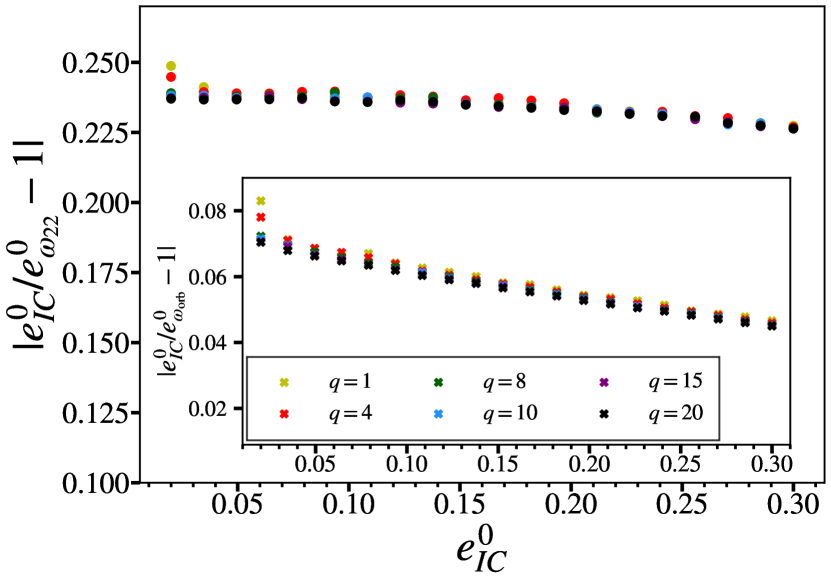
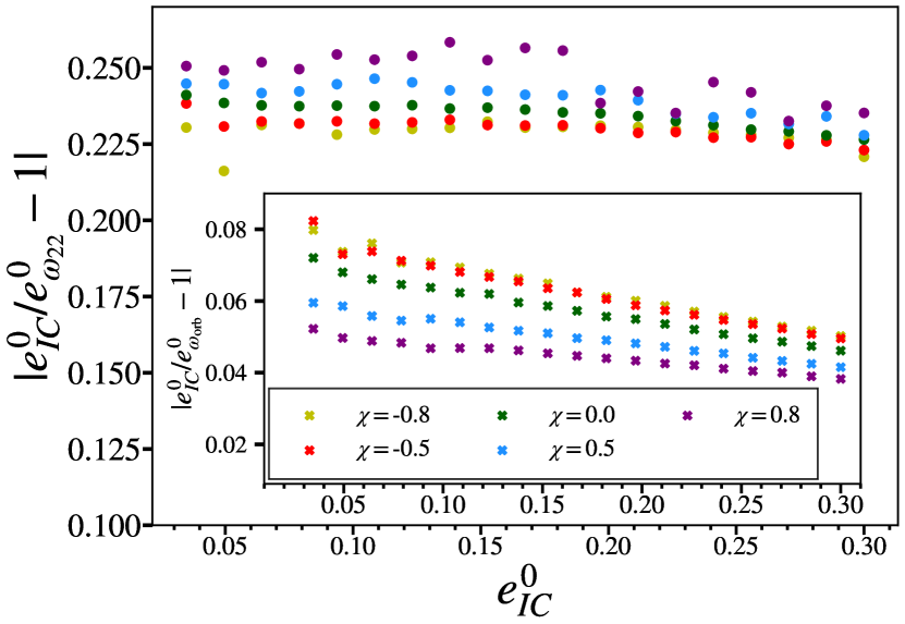
Figure 1: Top panel: Relative difference between the initial eccentricity from the initial conditions of SEOBNRv4EHM, $e^{0}_{IC}$, and the initial eccentricity computed from the frequency of the $(2,2)$ mode, $e^{0}_{\omega_{22}}$, of SEOBNRv4EHM as a function of $e^{0}_{IC}$ in the range $[0.02,0.3]$ for non-spinning configurations with mass ratios $q=\{1,4,8,10,15,20\}$. Lower panel: Same quantity as in the upper panel for a configuration with fixed mass ratio $q=2$, same range of $e^{0}_{IC}$, and distinct equal-spin values $\chi_{1}=\chi_{2}=\{-0.8,-0.5,0,0.5,0.8\}$. The insets of both panels show the relative difference between $e^{0}_{IC}$ and the eccentricity measured from the orbital frequency of SEOBNRv4EHM $e^{0}_{\omega_{\text{orb}}}$, for the same configurations as in the larger panels.

Starting at periastron ($\zeta=0$), we produce a sample of $5\times 10^{5}$ points randomly distributed in the parameter space $q\in[1,20]$, $\chi_{1,2}\in[-0.9,0.9]$ and $e^{\text{IC}}_{0}\in[0.01,0.3]$, and compute the relative difference between $e^{0}_{IC}$ and $e^{0}_{\omega_{22}}$ or $e^{0}_{\omega_{\text{orb}}}$. In the upper panel of Fig. 1, we show the relative difference between $e^{\text{IC}}_{0}$ and $e^{0}_{\omega_{22}}$ for some non-spinning configurations with mass ratios $q=\{1,4,8,10,15,20\}$. For the same cases we show in the inset of Fig. 1 the relative difference between $e^{0}_{IC}$ and $e^{0}_{\omega_{\text{orb}}}$. We observe that the relative difference for $e^{0}_{\omega_{22}}$ is $\sim 24\%$, while for $e^{0}_{\omega_{\text{orb}}}$ is significantly lower $\sim 6\%$. Moreover, the dependence on mass ratio is smaller than $1\%$, in relative difference, with the exception of the lower eccentricity cases where the measurement of the eccentricity has also a larger error, which we estimate to be $\sim 3\%$. We also note that with increasing values of $e^{0}_{IC}$ the relative differences decrease, especially for the eccentricity measured from the orbital frequency.

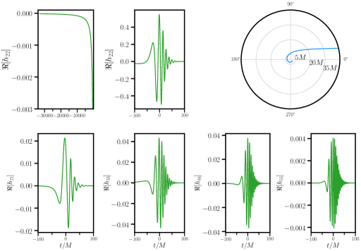
Figure 2: Waveform characteristics for a mass ratio $q=1.5$ non-spinning configuration with initial parameters $r_{0}=10^{4}M$, ${p_{\phi}}_{0}=3.97$ and $E_{0}/M=1.012$. Top row: From left to right, the two first panels show the real part of the 22-mode waveform in time domain, the first plot displays the full domain of the waveform while the second one zooms in into the merger part. The third panel displays the trajectory $r(\varphi)$ in polar coordinates. Each circle corresponds to a constant value of the orbital separation, which is marked on the figure. Bottom row: From left to right, the real part of the $(2,1),(3,3),(4,4),(5,5)$ modes in time domain zooming in close to the merger and ringdown regions.

In the lower panel of Fig. 1, we fix the mass ratio $q=2$, and vary the spin values $\chi_{1}=\chi_{2}=\{-0.8,-0.5,0,0.5,0.8\}$ for the same range of initial eccentricities as in the upper panel. The results show that the relative error between $e^{0}_{\omega_{22}}$ and $e^{0}_{IC}$ is $\sim 22\mbox{--}25\%$ when varying the spin values. These variations are quite similar to the results obtained when varying the mass ratios. The relative error between $e^{0}_{\omega_{\text{orb}}}$ and $e^{0}_{IC}$ is $\sim 5\mbox{--}8\%$, which is also very close in magnitude to the non-spinning case. However, in the lower panel of Fig. 1, one can appreciate that the relative errors vary more with spins than with mass ratio, specifically for positive spins the relative errors with respect to $e^{0}_{\omega_{22}}$ are $1\mbox{--}2\%$ larger than for negative spins, while the relative errors for $e^{0}_{\omega_{\text{orb}}}$ follow the inverse dependence with spins.

When considering the larger dataset of $5\times 10^{5}$ configurations, we find that the relative error between $e^{\text{IC}}_{0}$ and $e^{0}_{\omega_{22}}$ has an average of $\sim 30\%$ error, with the largest difference of $40\%$ for low eccentricities, where the errors in measuring the eccentricity are also larger due to the difficulties in determining the maxima and minima. For the relative error between $e^{\text{IC}}_{0}$ and $e^{0}_{\omega_{\text{orb}}}$, the average value is $\sim 6\%$, reaching up to $\sim 14\%$ for low values of the eccentricities. The results show a better agreement between $e^{0}_{IC}$ and $e^{0}_{\omega_{\text{orb}}}$ than between $e^{0}_{IC}$ and $e^{0}_{\omega_{22}}$. The relation between these different definitions of eccentricity can be derived using PN theory, and it will be presented in future work Ramos-Buades (In preparation.).

We note that the results reported in Fig. 1 quantify differences between the eccentricity specified in the SEOBNRv4EHM model and two other possible definitions of the eccentricity. We remark that even though there is no unique definition of the eccentricity, this kind of quantitative analysis will be required in future parameter-estimation analysis of eccentric GW sources with the LIGO, Virgo and KAGRA detectors in order to reliably compare the results among different eccentric waveform models.

Finally, we have also implemented hyperbolic-orbit initial conditions for the SEOBNRv4EHM model. The hyperbolic initial conditions are specified by the initial energy $E_{0}$ and angular momentum ${p_{\phi}}_{0}$ at infinity, which in practice we take at an initial orbital separation $r_{0}=10^{4}M$. We fix a value of the angular momentum ${p_{\phi}}_{0}$, and choose a value of the initial energy $E_{0}/M$. The choice of $E_{0}/M$ is typically done between the energy with zero radial momentum $E_{\text{min}}=H_{\text{EOB}}(r_{0},{p_{\phi}}_{0},{p_{r_{*}}}_{0}=0)$ and the energy at the last stable circular orbit (LSO) $E_{\text{max}}=H_{\text{EOB}}(r_{\text{LSO}},{p_{\phi}}^{\text{LSO}},{p_{r^{*}}^{\text{LSO}}})$ Damour et al. (2014); Nagar et al. (2021b); Gamba et al. (2021b). Then, we solve the following equation for $p_{{r_{*}}_{0}}$,

$$E_{0}\equiv H_{\text{EOB}}(r_{0},{p_{\phi}}_{0},{p_{r_{*}}}_{0}).$$ (19)

This procedure to set the initial conditions for hyperbolic orbits is very similar to the one used in the literature Damour et al. (2014); Nagar et al. (2021b), although we note that others are possible, for instance, one could express the initial conditions in terms of the initial velocity and impact parameter Bini et al. (2017); Cho et al. (2018); Mukherjee et al. (2021). In Fig. 2, we show the trajectory of a dynamical capture, as well as, the real part of the different multipoles in the SEOBNRv4EHM model. Although the model is able to reproduce the behavior of dynamical captures and hyperbolic encounters, we focus in this paper on the eccentric bound orbit case, and leave a thorough and quantitative analysis of the hyperbolic orbits, including comparison to NR results to the future.

III Performance of the multipolar eccentric effective-one-body waveform model

In this section, we first assess the accuracy of the multipolar eccentric waveform model SEOBNRv4EHM against the quasi-circular and eccentric NR waveforms at our disposal, using the faithfulness function, which is a metric introduced to quantify the closeness of two waveforms. Then, we explore the robustness and validity of the SEOBNRv4EHM model in the region of parameter space where we do not yet have NR waveforms. Finally, we evaluate the unfaithfulness between IMR eccentric waveforms and quasi-circular ones to estimate in which part of the parameter space and for which values of the eccentricity we expect large biases in recovering the source’s properties if quasi-circular orbit waveforms were used.

III.1 Faithfulness function

The GW signal emitted by an eccentric aligned-spin BBH system depends on 13 parameters. In Sec. II.3, we have introduced the $6$ intrinsic parameters describing the source properties of such a system. There are 7 additional parameters which relate the source and detector frames, notably the angular position of the line of sight measured in the source frame ($\iota$, $\varphi_{0}$), the sky location of the source in the detector frame $(\theta,\phi)$, the polarization angle $\psi$, the luminosity distance of the source $D_{L}$ and the time of arrival $t_{c}$.

The signal measured by the detector takes the form:

$$\begin{split}h(t)=&F_{+}(\theta,\phi,\psi)h_{+}(\iota,\varphi_{0},D_{L},\bm{\Theta},t_{c};t)\\ &+F_{\times}(\theta,\phi,\psi)h_{\times}(\iota,\varphi_{0},D_{L},\bm{\Theta},t_{c};t),\end{split}$$ (20)

where $\bm{\Theta}=\{m_{1,2},\chi_{1,2},e,\zeta\}$, and $F_{+}(\theta,\phi,\psi)$ and $F_{\times}(\theta,\phi,\psi)$ are the antenna-pattern functions Sathyaprakash and Dhurandhar (1991); Finn and Chernoff (1993). Equation (20) can be written in terms of an effective polarization angle $\kappa(\theta,\phi,\psi)$ as

$$h(t)=\mathcal{A}(\theta,\phi)\left[h_{+}\cos\kappa+h_{+}\sin\kappa\right],$$ (21)

where the definition of $\mathcal{A}(\theta,\phi)$ can be found in Refs. Cotesta et al. (2018); Ossokine et al. (2020), and we have removed the dependences of $\kappa$, $h_{+}$ and $h_{\times}$ to ease the notation. The GW polarizations can be decomposed as

$$h_{+}-ih_{\times}=\sum^{\infty}_{l=2}\sum_{m=-l}^{m=+l}{}_{-2}Y_{lm}(\varphi,\iota)\,h_{lm}(\bm{\Theta};t),$$ (22)

where $h_{lm}(\bm{\Theta};t)$ represents the gravitational waveform modes, and $Y^{-2}_{lm}(\varphi,\iota)$ are the -2 spin-weighted spherical harmonics.

We introduce the inner product between two waveforms $h_{1}$ and $h_{2}$ Sathyaprakash and Dhurandhar (1991); Finn and Chernoff (1993) as

$$\langle h_{1}|h_{2}\rangle=4\Re\int^{f_{\text{max}}}_{f_{\text{min}}}\frac{\hat{h}_{1}(f)\hat{h}^{*}_{2}(f)}{S_{n}(f)}df,$$ (23)

where the star denotes complex conjugate, the hat the Fourier transform, and $S_{n}(f)$ is the one-sided power-spectral density (PSD) of the detector noise. In this work we use the Advanced LIGO’s zero-detuned high-power design sensitivity curve Barsotti et al. (2018). When both waveforms are in band, we use $f_{\text{min}}=10$Hz and $f_{\text{max}}=2048$Hz, as the lower and upper bounds of the integral. For NR waveforms where this is not the case, we set $f_{\text{min}}=1.05f_{\text{start}}$, where $f_{\text{start}}$ is the starting frequency of the NR waveform.

The agreement between two waveforms — for example, the signal, $h_{s}$, and the template, $h_{t}$, observed by a detector, can be assessed by computing the faithfulness function Cotesta et al. (2018); Ossokine et al. (2020),

$$\mathcal{F}(M_{\textrm{s}},\iota_{\textrm{s}},{\varphi_{0}}_{\textrm{s}},\kappa_{\textrm{s}})=\max_{t_{c},{\varphi_{0}}_{t},\kappa_{t}}\left[\left.\frac{\langle h_{s}|h_{t}\rangle}{\sqrt{\langle h_{s}|h_{s}\rangle\langle h_{t}|h_{t}\rangle}}\right|_{\begin{subarray}{c}\iota_{\mathrm{s}}=\iota_{t}\\ \bm{\Theta}_{\mathrm{s}}(t_{\mathrm{s}}=t_{0_{\mathrm{s}}})=\bm{\Theta}_{t}(t_{t}=t_{0_{\mathrm{t}}})\end{subarray}}\right].$$ (24)

In Eq. (24) the inclination angle of the signal and the template are set to be the same, while the coalescence time, azimuthal angle and effective polarization angle of the template $(t_{0_{t}},\varphi_{0_{t}},\kappa_{t})$, are adjusted to maximize the faithfulness of the template. This is a typical choice made when comparing waveforms with higher-order modes Cotesta et al. (2018); Ossokine et al. (2020); García-Quirós et al. (2020). It is convenient to introduce the sky-and-polarization averaged faithfulness to reduce the dimensionality of the faithfulness function and express it in a more compact form Cotesta et al. (2018); Ossokine et al. (2020),

$$\overline{\mathcal{F}}(M_{\textrm{s}})=\frac{1}{8\pi^{2}}\int^{1}_{-1}d{(\cos\iota_{\textrm{s}})}\int^{2\pi}_{0}d{\varphi_{0}}_{\textrm{s}}\int^{2\pi}_{0}d\kappa_{\textrm{s}}\mathcal{F}(M_{\textrm{s}},\iota_{\textrm{s}},{\varphi_{0}}_{\textrm{s}},\kappa_{\textrm{s}}).$$ (25)

Another useful metric to assess the closeness between waveforms is the signal-to-noise (SNR)-weighted faithfulness Ossokine et al. (2020)

$$\overline{\mathcal{F}}_{\mathrm{SNR}}(M_{\mathrm{s}})=\sqrt[3]{\frac{\int^{1}_{-1}d{(\cos\iota_{\textrm{s}})}\int_{0}^{2\pi}d\kappa_{\mathrm{s}}\int_{0}^{2\pi}d{\varphi_{0}}_{\mathrm{s}}\ \mathcal{F}^{3}(M_{\textrm{s}},\iota_{\textrm{s}},{\varphi_{0}}_{\textrm{s}},\kappa_{\textrm{s}})\ \mathrm{SNR}^{3}(\iota_{\textrm{s}},{\varphi_{0}}_{\textrm{s}},\kappa_{\textrm{s}})}{\int^{1}_{-1}d{(\cos\iota_{\textrm{s}})}\int_{0}^{2\pi}d\kappa_{\mathrm{s}}\int_{0}^{2\pi}d{\varphi_{0}}_{\mathrm{s}}\ \mathrm{SNR}^{3}(\iota_{\textrm{s}},{\varphi_{0}}_{\textrm{s}},\kappa_{\textrm{s}})}},$$ (26)

where the SNR is defined as

$$\mathrm{SNR}(\iota_{\textrm{s}},{\varphi_{0}}_{\textrm{s}},\theta_{\textrm{s}},\phi_{\textrm{s}},\kappa_{\textrm{s}},{D_{\mathrm{L}}}_{\mathrm{s}},\bm{\Theta}_{\mathrm{s}},{t_{c}}_{\mathrm{s}})\equiv\sqrt{\left(h_{\mathrm{s}},h_{\mathrm{s}}\right)}.$$ (27)

In Eq. (26) the weighting by the SNR takes into account the dependence on the phase and effective polarization of the signal at a fixed distance. Finally, we introduce the unfaithfulness or mismatch as

$$\overline{\mathcal{M}}=1-\overline{\mathcal{F}}.$$ (28)

III.2 Comparison against quasi-circular numerical-relativity waveforms

We begin by assessing the accuracy of the SEOBNRv4EHM waveform model in the zero eccentricity limit, focusing on the unfaithfulness against the set of quasi-circular NR waveforms used to calibrate and validate the SEOBNRv4HM model. The public NR waveforms are available in the SXS waveform catalog Boyle et al. (2019) produced with the Spectral Einstein code (SpEC) SpE . The parameters of the public and non-public 141 NR waveforms are listed in the Appendix F of Ref. Cotesta et al. (2018).

In order to simplify our analysis, we restrict first to the $(2,|2|)$-modes waveforms, and then include higher order modes. For the dominant $(2,|2|)$-modes the faithfulness can be simplified with respect to Eq. (24) as the inclination angle of the signal is not usually considered due to the angular dependence of the ${}_{-2}Y_{2\pm 2}$ harmonics, and the fact that $\kappa$, $\iota$ and $\varphi$ are degenerate  Capano et al. (2014). Therefore, the faithfulness function for the quasi-circular $(2,|2|)$-modes waveforms can be expressed as

$$\mathcal{F}_{22}(M_{\textrm{s}},{\varphi_{0}}_{\textrm{s}})=\max_{t_{c},{\varphi_{0}}_{t}}\left[\left.\frac{\langle h_{s}|h_{t}\rangle}{\sqrt{\langle h_{s}|h_{s}\rangle\langle h_{t}|h_{t}\rangle}}\right|_{\begin{subarray}{c}\bm{\Theta}_{\mathrm{s}}(t_{\mathrm{s}}=t_{0_{\mathrm{s}}})=\bm{\Theta}_{t}(t_{t}=t_{0_{\mathrm{t}}})\end{subarray}}\right].$$ (29)

In practice, we remove the dependence of the faithfulness on the azimuthal angle of the signal by evaluating Eq. (29) in a grid of 8 values for ${\varphi_{0}}_{\textrm{s}}\in[0,2\pi]$, and averaging the result to obtain $\overline{\mathcal{F}}_{22}$. The optimization over the coalescence time of the signal is efficiently computed by applying an inverse Fourier Transform Allen et al. (2012) and we analytically optimize over the coalescence phase of the template Capano et al. (2014). From Eq. (29) one can define the mismatch or unfaithfulness as,

$$\overline{\mathcal{M}}_{22}=1-\overline{\mathcal{F}}_{22}.$$ (30)

The condition $\bm{\Theta}_{\mathrm{s}}(t_{\mathrm{s}}=t_{0_{\mathrm{s}}})=\bm{\Theta}_{t}(t_{t}=t_{0_{\mathrm{t}}})$ in Eq. (29) enforces that the intrinsic parameters of both the template and the signal are the same at the start of the waveform $t=t_{0}$. This implies that the component masses $m_{1,2}$, or equivalently the mass ratio $q=m_{1}/m_{2}\geq 1$ and the total mass $M=m_{1}+m_{2}$, and the dimensionless spins $\chi_{1,2}$ of the signal and the template are identical at $t_{0}$ Ossokine et al. (2020).

For the calculation of the unfaithfulness we consider a total-mass range of $20M_{\odot}\leq M\leq 200M_{\odot}$. We show in Fig. 3 the $22-$mode unfaithfulness maximized over the total-mass range for the SEOBNRv4 and SEOBNRv4E models. We remind that the SEOBNRv4 model was calibrated requiring an unfaithfulness for the $22$-mode against the 141 NR waveforms of at most of $1\%$. It is interesting to note that the SEOBNRv4E eccentric model achieves a similar accuracy, with the median of the distribution slightly larger than the one of the SEOBNRv4 model. This is due to the fact that the SEOBNRv4E model contains eccentric corrections, which were not available when calibrating the SEOBNRv4 model to NR in the quasi-circular limit.

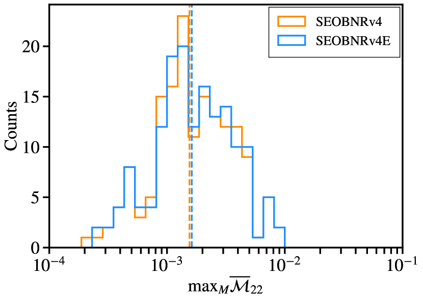
Figure 3: Distribution of the maximum unfaithfulness of SEOBNRv4 (orange) Bohé et al. (2017) and the new SEOBNRv4E (blue) against the public 141 quasi-circular NR simulations of Ref. Bohé et al. (2017). The total mass range considered is $20M_{\odot}\leq M\leq 200M_{\odot}$. The calculations are done with the Advanced LIGO’s zero-detuned high-power design sensitivity curve Barsotti et al. (2018). The vertical dashed orange (blue) lines correspond to the median values of the SEOBNRv4 (SEOBNRv4E) distributions.

The higher order multipoles included in SEOBNRv4EHM are the same as in SEOBNRv4HM (i.e., $(l,|m|)=\{(2,1),(3,3),(4,4),(5,5)\}$). When computing the unfaithfulness of the models with higher modes against NR, we include in the NR waveforms all the modes with $l\leq 5$ as done in Ref. Cotesta et al. (2018). To ease the visualization of the results, we compute the SNR-weighted mismatches defined in Eq. (26), and average over the signal inclination, azimuthal and effective polarization angles. In practice, the average is performed over three different inclination angles of the signal $\iota_{s}=\{0,\pi/3,\pi/2\}$, and for each inclination angle we make a grid of $8\times 8$ for $\kappa_{s},\varphi_{0s}\in[0,2\pi]$. In Fig. 4, we show the SNR-weighted mismatches for the SEOBNRv4HM and SEOBNRv4EHM models against the quasi-circular NR waveforms at our disposal. Again, we note that the mismatches of the SEOBNRv4EHM model are very similar to the ones of the SEOBNRv4HM model. There are a few cases at high total masses for which both models have unfaithfulness above $1\%$, but not larger than $1.5\%$, as reported also in Ref. Cotesta et al. (2018). This indicates that the higher-order modes in the eccentric model have a comparable accuracy to the ones of the underlying quasi-circular model in the zero eccentricity limit.

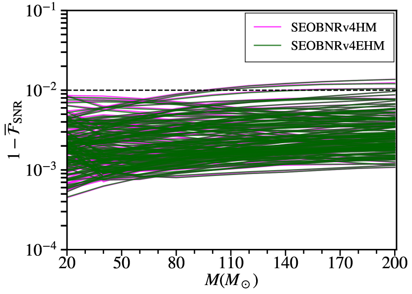
Figure 4: SNR-weighted unfaithfulness, as defined in Eq. (28), as a function of the total mass, in the range $20M_{\odot}\leq M\leq 200M_{\odot}$, between the SEOBNRv4HM (pink) and SEOBNRv4EHM (green) models and the SXS quasi-circular NR waveforms used in Ref. Cotesta et al. (2018). The calculations are done with the Advanced LIGO’s zero-detuned high-power design-sensitivity curve Barsotti et al. (2018), which is an estimate for the upcoming O4 run. The horizontal black dashed line indicates the $1\%$ unfaithfulness value.

III.3 Comparison against eccentric numerical-relativity waveforms

The calculation of the unfaithfulness assumes that the intrinsic parameters of both template and signal are identical at the start of the evolution, that is we use the condition $\bm{\Theta}_{\mathrm{s}}(t_{\mathrm{s}}=t_{0_{\mathrm{s}}})=\bm{\Theta}_{t}(t_{t}=t_{0_{\mathrm{t}}})$ in Eq. (24). In the eccentric case, this would imply that the mass ratio, $q$, total mass, $M$, dimensionless spins, $\chi_{1,2}$, eccentricity, $e$ and relativistic anomaly, $\zeta$, of both the signal and the template are the same at the start of the waveform. While the spins and mass parameters are uniquely fixed in the non-precessing spinning case, the eccentricity and relativistic anomaly cannot be uniquely identified with respect to the NR waveforms. Consequently, when comparing a waveform model against eccentric NR waveforms , an optimization over the initial eccentricity and relativistic anomaly has to be performed to take into account the different definition of eccentricity between the model and the NR waveforms.

In the case of the SEOBNRv4EHM model, to reduce the dimensionality of the parameter space, we use the initial conditions for eccentric orbits starting at periastron ($\zeta=0$), and we compute the eccentric EOB waveforms by specifying the initial eccentricity, $e_{0}$, and starting frequency, $\omega_{0}$. Thus, when computing the faithfulness of the model against eccentric NR waveforms we have to maximize over $e_{0}$ and $\omega_{0}$. Furthermore, here we compute the unfaithfulness using also another publicly available eccentric EOB model, TEOBResumSE  Chiaramello and Nagar (2020); Nagar et al. (2021a); Nagar and Rettegno (2021); Placidi et al. (2021), for which we also specify initial conditions at periastron, and optimize over the initial eccentricity and starting frequency of the model. We note that although the TEOBResumSE can include higher-order modes, we use here only the $(2,|2|)$-modes, as we have found that in the presence of eccentricity some of the higher-order modes develop unphysical behaviors close to merger and ringdown. These features are likely due the treatment of the NQC corrections in the eccentric case, as already reported in Ref. Nagar and Rettegno (2021).

First, we focus on the $(2,|2|)$-modes only waveforms. We define the eccentric faithfulness function as follows,

$$\mathcal{F}^{\text{ecc}}_{22}(M_{\textrm{s}},{\varphi_{0}}_{\textrm{s}})=\max_{t_{0_{t}},{\varphi_{0}}_{t},e_{0},\omega_{0}}\left[\left.\frac{\langle h_{s}|h_{t}\rangle}{\sqrt{\langle h_{s}|h_{s}\rangle\langle h_{t}|h_{t}\rangle}}\right|_{\begin{subarray}{c}\bm{\Theta}_{\mathrm{s}}(t_{\mathrm{s}}=t_{0_{\mathrm{s}}})=\bm{\Theta}_{t}(t_{t}=t_{0_{\mathrm{t}}})\end{subarray}}\right].$$ (31)

For completeness, we introduce here also the unfaithfulness function as

$$\overline{\mathcal{M}}^{\text{ecc}}_{22}=1-\overline{\mathcal{F}}^{\text{ecc}}_{22}.$$ (32)

From Eq. (31) one observes that in the eccentric case two additional numerical optimizations have to be performed, as compared to the quasi-circular case (see Eq. (29)). The main difficulty of estimating such optimal values arises from the fact that the two additional optimizations cannot be easily performed with standard optimization algorithms, as the unfaithfulness has a highly oscillatory behavior as a function of these parameters. This can be observed in Fig. 5 where we show the unfaithfulness of the SEOBNRv4E waveform against the SXS:BBH:1355 waveform as function of the starting frequency. In Fig. 5, the mismatch is computed for a total mass of $20M_{\odot}$ and at fixed initial eccentricity $e_{0}=0.09$ for the SEOBNRv4E model. The high number of local maxima and minima in the unfaithfulness function makes standard optimization algorithms quite inefficient, and it increases substantially the computational cost of such procedure.

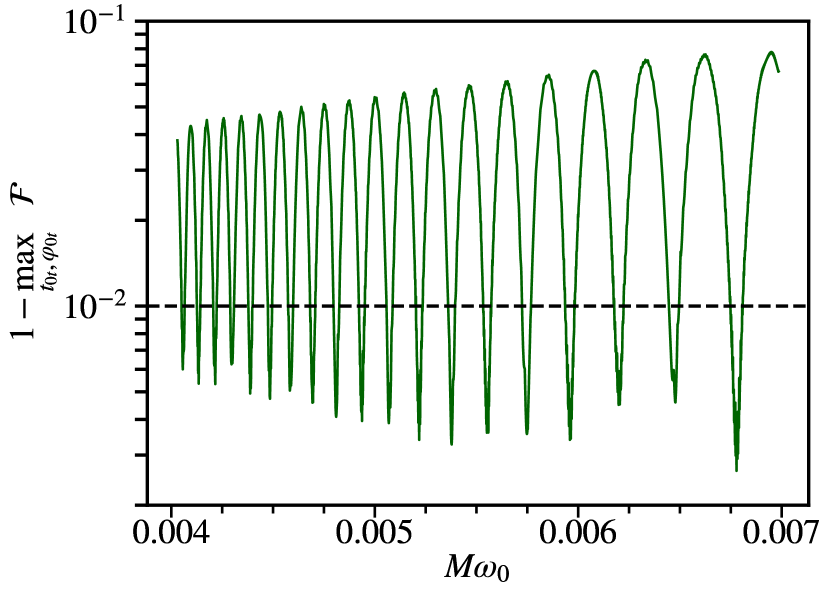
Figure 5: Unfaithfulness of the SEOBNRv4E waveform model against the SXS:BBH:1355 waveform at a fixed initial eccentricity, $e_{0}=0.09$, as a function of the starting frequency of the model $M\omega_{0}$. The unfaithfulness is computed at a fixed total mass of $20M_{\odot}$, maximizing over the coalescence time, $t_{0_{t}}$, and azimuthal angle, $\varphi_{0_{t}}$, of the model.

In order to overcome this problem, different eccentric EOB models use different approaches to estimate the optimal values for $e_{0}$ and $\omega_{0}$. In the case of the SEOBNREHM model Cao and Han (2017); Liu et al. (2020, 2021) (not to be confused with our SEOBNRv4EHM model here), the starting frequency is set to the frequency when the eccentricity is estimated from the NR waveforms, and then the initial eccentricity is varied to get the best match against the NR waveforms. While for the TEOBResumSE model, the eccentricity and starting frequency are varied manually to get the lowest unfaithfulness against NR Nagar et al. (2021a).

Here, we develop an automatic procedure to perform the two optimizations over $e_{0}$ and $\omega_{0}$. The procedure is as follows:

• Fix the total mass to the lower bound of the total mass range used, that is $20M_{\odot}$. In this way, we ensure that more inspiral part of the NR waveform is in the frequency band of the mismatch calculation.

• Create a grid in eccentricity of $N_{e}$ values around the value of the eccentricity as measured from the NR orbital frequency using Eq. (18), $e^{\text{NR}}_{\omega_{\text{orb}}}$, such that $e_{0}\in[e^{\text{NR}}_{\omega_{\text{orb}}}-\delta e,e^{\text{NR}}_{\omega_{\text{orb}}}+\delta e]$. The value of $\delta e$ determines the eccentricity interval. In the case $e^{\text{NR}}_{\omega_{\text{orb}}}-\delta e<0$, we take the lower bound to be zero.

• For each value of the eccentricity, generate a grid of $N_{\omega}$ values of starting frequency. The upper bound is determined by the frequency at which the EOB waveform equals the length $l$ of the eccentric NR waveform, $\omega^{l_{\text{NR}}=l_{\text{EOB}}}_{0}$, while the lower bound is determined by a chosen $\delta\omega$. Thus, the frequency grid is $\omega_{0}\in[\omega^{l_{\text{NR}}=l_{\text{EOB}}}_{0}-\delta\omega,\omega^{l_{\text{NR}}=l_{\text{EOB}}}_{0}]$.

• For each point in the grid, compute the unfaithfulness optimizing over the time shift and phase offset of the template as in Eq. (29).

• Store the values $(e^{\text{opt}}_{0},\omega^{\text{opt}}_{0})$ which provide the lowest unfaithfulness.

• In order to reduce the computational cost, we use the optimal values, $(e^{\text{opt}}_{0},\omega^{\text{opt}}_{0})$ at $20M_{\odot}$ for the whole mass range.

For the results in this paper we choose $N_{e}=200$, $N_{f}=500$, an eccentricity interval, $\delta e=0.1$, and a starting frequency interval of $\delta f=10$Hz at $20M_{\odot}$, which translates into $\delta\omega=0.006$.

The above optimization procedure is tested by computing the unfaithfulness against the eccentric NR waveforms publicly available in the SXS catalog Hinder et al. (2018); Boyle et al. (2019). In Table 1 we summarize the main properties of the NR simulations used in this work, the optimal values of initial eccentricity and starting frequency of the SEOBNRv4E and TEOBResumSE models, and the maximum value over total mass range of the unfaithfulness of the models against the NR simulations. We note that there is a particular simulation SXS:BBH:1169 for which the optimization procedure leads to zero initial eccentricity for TEOBResumSE. This is a NR simulation with very low eccentricity for which the quasi-circular waveform has already a very low mismatch of $0.78\%$. The reported value of the unfaithfulness of TEOBResumSE for this case in Table 1 is slightly lower than that reported in Refs. Nagar et al. (2021a); Nagar and Rettegno (2021). We have checked modifications of the grid parameters in the eccentricity and starting frequency grids for the optimization procedure, particularly increasing the resolution up to $N_{e}=300$ and $N_{f}=1000$, but this optimal eccentricity value of zero still remains unchanged. While it is possible that further increasing the resolution could lead to a slightly lower unfaithfulness, it also significantly increases the computational cost and therefore we opt to use the already calculated value. We also note that for this particular case (which has low eccentricity and high spins) the optimization procedure may be affected by the slight discontinuity of the TEOBResumSE model for small eccentricities as already noted in Ref. O’Shea and Kumar (2021).

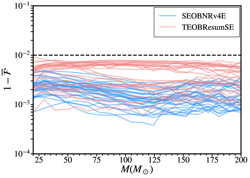
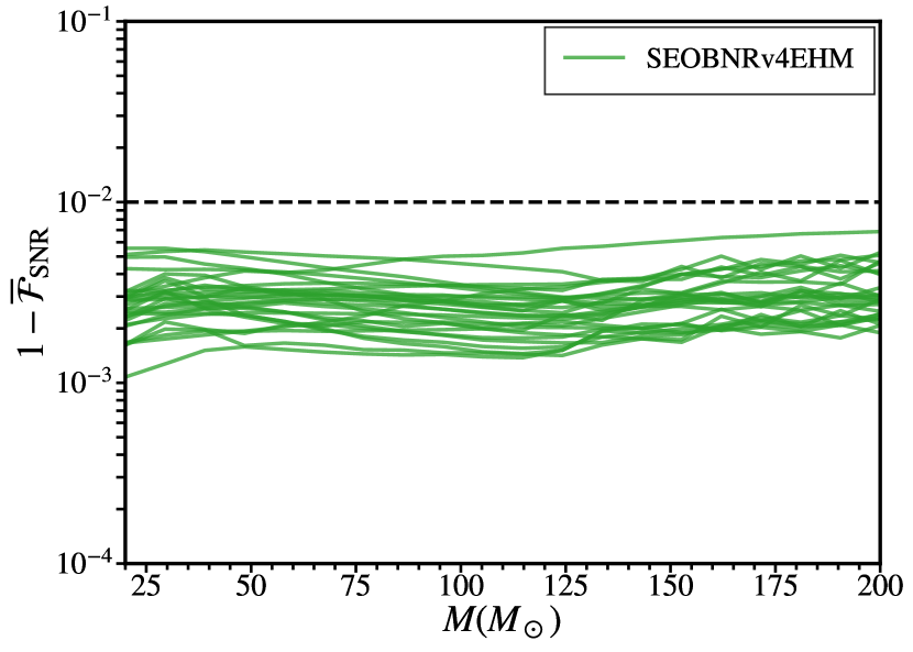
Figure 6: Upper panel: Unfaithfulness of the SEOBNRv4E and TEOBResumSE models against the 28 eccentric public SXS simulations listed in Table 1. The calculations are performed optimizing over the initial eccentricity and starting frequency at periastron. Lower panel: Unfaithfulness of SEOBNRv4EHM model against the same NR waveforms as in the upper panel, but including all modes with $l\leq 5$ in the NR waveforms. The calculations are performed using the optimal values of eccentricity and starting frequency obtained from the unfaithfulness computed with SEOBNRv4E. The horizontal dashed lines in both panels indicate the $1\%$ value of unfaithfulness.

The unfaithfulness of the SEOBNRv4E and TEOBResumSE models against the dataset of eccentric NR waveforms described in Table 1 are shown in the upper panel of Fig. 6. We note that the unfaithfulness curves are always below $1\%$ for the whole dataset and total mass ranges. These results also indicate that the approximation in step 6) of using the same optimal values for $(e^{\text{opt}}_{0},\omega^{\text{opt}}_{0})$ for the whole total mass range is reasonable, as the unfaithfulness does not significantly increase with the total mass range. The bulk of the unfaithfulness curves for the SEOBNRv4E model is below the ones of the TEOBResumSE model for the NR dataset considered here. We note that the values of the unfaithfulness for the TEOBResumSE model reported here are similar to the ones in Ref. Nagar et al. (2021a). However, in recent publications Nagar and Rettegno (2021); Placidi et al. (2021), lower unfaithfulnesses are reported for the TEOBResumSE model, driven by recalibrating it to quasi-circular NR waveforms, and by better computing the Fourier transform of the time-domain waveforms, as remarked in Refs. Nagar and Rettegno (2021); Placidi et al. (2021). (This improved model is not public.) As a consequence of those improvements, the main bulk of the unfaithfulness curves is closer to $10^{-3}$ values, and thus, at a similar level as the SEOBNRv4E model in Fig. 6. We remark that in order to better assess the accuracy of both models, comparisons against larger datasets of eccentric NR simulations are required. Eventually, Bayesian inference analyses will be needed to assess biases in the recovered parameters.

The calculation of the unfaithfulness including higher order modes requires three numerical optimizations (initial eccentricity, starting frequency and azimuthal angle of the template) and an analytical optimization over the effective polarization angle for each single point in the sky of the signal. Consequently, computing SNR-weighted unfaithfulness averaged over the sky-positions, orientations and inclinations of the signal becomes computationally prohibitive. In order to reduce the computational cost, we assume that the optimal values for the initial eccentricity and starting frequency of the SEOBNRv4EHM model are the same as the ones obtained for the SEOBNRv4E model, $(e^{\text{opt}}_{0},\omega^{\text{opt}}_{0})$, and we compute the unfaithfulness as in the quasi-circular case, numerically optimizing over the azimuthal angle of the template, and analytically over the effective polarization angle of the template.

We apply this approximation and compute the unfaithfulness between the SEOBNRv4EHM waveforms and the eccentric NR waveforms, which include all the modes with $l\leq 5$. We show the results in the lower panel of Fig. 6. We can observe that the curves of the SNR-weighted unfaithfulness for the multipolar model are always below $1\%$. This indicates that the approximation of using the optimal values of $(e^{\text{opt}}_{0},\omega^{\text{opt}}_{0})$ obtained from the unfaithfulness of the SEOBNRv4E model is a good approximation. When comparing the unfaithfulness of the SEOBNRv4EHM model against the SEOB model developed in Ref. Liu et al. (2021) (SEOBNREHM), we find that the unfaithfulness of SEOBNRv4EHM are always smaller than $1\%$, which is not the case for the SEOBNREHM model, which presents some cases with unfaithfulness as large as $2\%$ Liu et al. (2021). We also note that the unfaithfulness for the SEOBNRv4EHM model is overall larger than that for the SEOBNRv4E model, this may indicate that the higher-order modes in the multipolar model are not as accurately modeled as the dominant $(2,2)$ mode. However, we remark that the procedure to compute the unfaithfulness for the model with higher-order modes is suboptimal as the values of $(e^{\text{opt}}_{0},\omega^{\text{opt}}_{0})$ are obtained from the SEOBNRv4E model, thus the unfaithfulness results for SEOBNRv4EHM are a conservative estimate. Furthermore, some higher-order modes in the dataset of the eccentric NR waveforms are affected by numerical noise, which may also affect the unfaithfulness values. This can also be seen in Fig. 7 where the different multipoles of the SEOBNRv4EHM waveform model for the optimal values of $(e^{\text{opt}}_{0},\omega^{\text{opt}}_{0})$, and of the NR waveform SXS:BBH:1364 are shown. We note that the higher-order modes of the model have very good agreement with respect to NR, and that the early inspiral of the NR (5,5)-mode is dominated by numerical noise. Thus, larger datasets of more accurate eccentric NR waveforms are required in order to better assess and improve the accuracy of multipolar eccentric EOB waveform models.

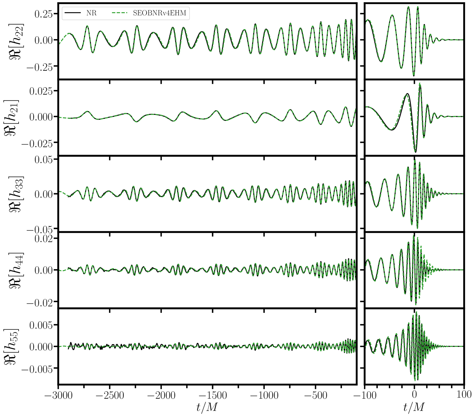
Figure 7: From top to bottom, real part of the (2,2),(2,1), (3,3), (4,4) and (5,5) modes in the time domain. The black curve corresponds to the NR simulation SXS:BBH:1369, which has mass ratio $q=2$, zero spins, and eccentricity $e_{\omega_{\text{orb,p}}}=0.257$, while the green curve corresponds to the SEOBNRv4EHM model for the values of eccentricity and starting frequency that lead to the lowest unfaithfulness for the (2,2) mode.

III.4 Robustness of the model across parameter space

Having assessed the accuracy of the model against the NR waveforms at our disposal, we now explore the region of validity of the SEOBNRv4EHM waveform model and identify the regions of parameter space where the model can be robustly generated.

One important property of a waveform model is its smoothness under small perturbations of the intrinsic parameters. In order to test this property, we compute the unfaithfulness between the SEOBNRv4E waveforms perturbing the eccentricity parameter by $\delta e=10^{-7}$. We perform this test using the pycbc_faithsim function in the PyCBC software Nitz et al. (2020) and employ for $10^{6}$ waveforms randomly distributed in the following parameter space: $\chi_{1,2}\in[-0.99,0.99]$, $q\in[1,20]$, $M\in[10,100]M_{\odot}$, $e_{0}\in[0,0.3]$. We choose $19$Hz for the starting frequency of the waveforms, and $20$Hz for the overlap calculations. We find that only a few cases have unfaithfulness above $10^{-8}$, with the maximum mismatch being $0.3\%$ and the median mismatch being $0$, indicating that the waveform model behaves smoothly under changes of the eccentricity parameter.

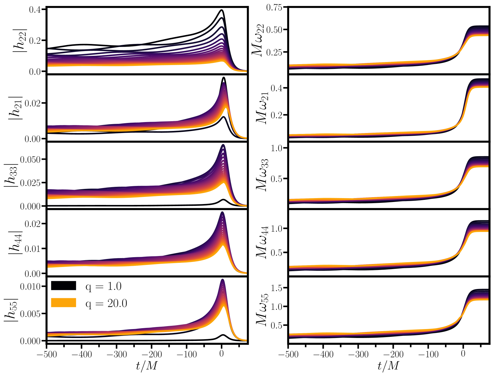
Figure 8: From top to bottom amplitudes (left panels) and frequencies (right panels) of the $(2,2)$, $(2,1)$, $(3,3)$, $(4,4)$ and $(5,5)$ modes of SEOBNRv4EHM versus time, aligned at merger, for a configuration with initial eccentricity $e_{0}=0.25$, spins $(\chi_{1},\chi_{2})=(0.5,-0.75)$, starting frequency $20$Hz and total mass $60M_{\odot}$, for a mass ratio range $q\in[1,20]$.

As an example, we show in Fig. 8 the amplitude and frequency of the multipoles in the SEOBNRv4EHM model (i.e., $(l,m)=\{(2,2),(2,1),(3,3),(4,4),(5,5)\}$ modes), as function of time and aligned at the merger time, for different values of the mass ratio, for a configuration with initial eccentricity $e_{0}=0.25$, spins $(\chi_{1},\chi_{2})=(0.5,-0.75)$, starting frequency $20$Hz and with total mass $60M_{\odot}$. As can be seen, the modes of the SEOBNRv4EHM model have a smooth behaviour in amplitude and frequency under variation of the mass ratio $q=1\mbox{--}20$. We note that, during the inspiral, in the equal-mass case, the amplitude of the odd-m modes (except the $(2,1)$ mode) is very small compared to the unequal-mass configurations. The same behavior is present in the amplitudes of the quasi-circular orbit SEOBNRv4HM model. As discussed in Ref. Cotesta et al. (2018) (see Fig. 2 and text around), this is due to the fact that this binary configuration has a relatively large asymmetric-spin parameter $\chi_{A}=(\chi_{1}-\chi_{2})/2=0.5$, for which, in the equal-mass (or nearly equal-mass) case the odd-m modes (except the $(2,1)$-mode) have very small amplitude during the inspiral, as predicted by PN theory.

We find that the orbit averaging procedure that we apply to the NQC function works quite well from large negative spins to mild positive spins, but binary’s configurations with large-positive spins and small initial separation (or large dimensionless orbital frequency) can challenge this procedure due to the last periastron passage occurring very close to merger (see the Appendix B). This can cause oscillations in the dynamical quantities in the late inspiral. In order to test the smoothness of the waveform model in the large-spin region, we compute the unfaithfulness between two waveforms varying the spins in the region $\chi_{1,2}\in[0.8,0.99]$ for 100 mass ratios $q\in[1,50]$. For each mass ratio, we compute the unfaithfulness between a waveform with $\chi_{1}=\chi_{2}=0.8$, initial eccentricity $0.3$ at starting frequency of 20Hz and total mass $100M_{\odot}$ and waveforms with the same parameters but varying both $\chi_{1,2}\in[0.8,0.99]$. This choice of total mass, starting frequency and eccentricity implies smaller initial separations of $r/M\sim 11$, and thus corresponds to a challenging case for the quasi-circular assumption of the merger-ringdown signal. The results from such a test show an oscillatory unfaithfulness surface across parameter space without sharp features. We also observe that for $\chi_{1,2}\gtrsim 0.9\mbox{--}0.95$ the frequency of the (2,2)-mode can have small spurious oscillations, thus, the model should be used with caution in this region of parameter space. Nevertheless, the model does not show prominent features in the waveform, and therefore, we recommend that it is used up to spins $0.99$, eccentricity $0.3$ and initial frequency up to $20$ Hz. We plan to improve the model in the transition from plunge to merger for large spins, as soon as we will have access to NR eccentric waveforms with large spins.

Figure 9: Plus gravitational polarization versus time for a $q=2$ non-spinning configuration computed with SEOBNRv4EHM for four different initial eccentricities $e_{0}=[0,0.3,0.5,0.8]$, and total mass $M=100M_{\odot}$. All the configurations have a starting frequency of $20$Hz at periastron. We note that for $e_{0}=0.8$ the waveform reproduces the burst-like features produced at the periastron passages.

We note that whereas we have probed the validity of the model through comparisons to the public SXS eccentric waveforms and internal consistency tests mostly for mass ratios $q\in[1,20]$ and eccentricities $e\in[0,0.3]$ at 20Hz, we can also generate SEOBNRv4EHM waveforms at higher eccentricities and mass ratios, as illustrated in Fig. 9, where we show the plus polarization $h_{+}$ for a non-spinning BBH with mass-ratio 2 and different initial eccentricities $e_{0}=[0,0.3,0.5,0.8]$. These configurations are produced with a starting frequency of 20Hz defined at periastron, so that, at that time, there are no frequencies in the inspiral higher than the starting frequency. In fact, we have checked that the model can be robustly generated at higher eccentricities by producing a large set of ($10^{6}$) waveforms randomly distributed in mass ratios $q\in[1,50]$, spins $\chi_{1,2}\in[-0.99,0.99]$, initial eccentricity $e_{0}\in[0.3,0.9]$ at a starting frequency of $20$Hz for binaries with total mass $80M_{\odot}$. In the generation of such dataset we do not find any waveform generation failure. However, lacking NR waveforms to compare against, we are not able to assess the accuracy and robustness of the model in this much larger region of the parameter space, so we recommend to use the model with caution for $e_{0}>0.3$.

Finally, we note that the region of parameter space with eccentricity up to $0.3$ at 20 Hz is is of significant astrophysical interest. In fact, it is expected that most of the GW events detected with ground-based detectors, such as LIGO, Virgo and KAGRA, have small eccentricities $\lesssim 0.1$ Wen (2003); Samsing (2018); Rodriguez et al. (2018); Zevin et al. (2021), which are typically defined at 10Hz.

The studies discussed in this section provide just a glance of all the internal checks performed to validate and implement the SEOBNRv4EHM waveform model in LALSuite The LIGO Scientific Collaboration (2015), so that it is available to the large GW community as a tool to carry out inference studies of GW signals.

Table 1: Summary of the eccentric NR simulations used in this work Hinder et al. (2018); Boyle et al. (2019). Each simulation is specified by the mass ratio $q=m_{1}/m_{2}\geq 1$, z-component of the dimensionless spin vectors, $\chi_{1,2}$, the NR orbital frequency $\omega_{\text{orb,p}}$, the eccentricity measured from the NR orbital frequency $e_{\omega_{\text{orb,p}}}$, the $(2,2)$-mode frequency $\omega_{22,p}$, and the eccentricity measured from the $(2,2)$-mode frequency $e_{\omega_{22,p}}$, all evaluated at first periastron passage. For each simulation we report also the optimal values of the starting orbital frequency and eccentricity at periastron, ($\omega_{p}$, $e_{\omega_{p}}$), for the SEOBNRv4E and TEOBResumSE waveform models, as well as the maximum mismatch over the total mass range using such optimal values against the NR waveforms.

	Numerical-relativity simulations							SEOBNRv4E			TEOBResumSE
ID	q	$\chi_{1}$	$\chi_{2}$	$\omega_{\text{orb,p}}$	$e_{\omega_{\text{orb,p}}}$	$\omega_{\text{22,p}}$	$e_{\omega_{\text{22,p}}}$	$\omega_{p}$	$e_{\omega_{p}}$	$1-\bar{\mathcal{F}}_{\text{max}}[\%]$	$\omega_{p}$	$e_{\omega_{p}}$	$1-\bar{\mathcal{F}}_{\text{max}}[\%]$
SXS:BBH:0089	1	-0.5	0.0	0.0128	0.06	0.025	0.048	0.0123	0.064	0.15	0.0111	0.064	0.64
SXS:BBH:0321	1	0.33	-0.44	0.0204	0.06	0.04	0.05	0.0196	0.07	0.22	0.0176	0.067	0.67
SXS:BBH:0322	1	0.33	-0.44	0.0223	0.075	0.0434	0.061	0.0224	0.086	0.35	0.0198	0.085	0.63
SXS:BBH:0323	1	0.33	-0.44	0.0235	0.126	0.045	0.102	0.0226	0.143	0.24	0.022	0.143	0.72
SXS:BBH:0324	1	0.33	-0.44	0.0303	0.246	0.0554	0.172	0.0299	0.297	0.3	0.0287	0.286	0.8
SXS:BBH:1136	1	-0.75	-0.75	0.0244	0.09	0.0475	0.076	0.0231	0.113	0.31	0.0209	0.113	0.24
SXS:BBH:1149	3	0.7	0.6	0.0197	0.048	0.0385	0.037	0.0189	0.045	0.3	0.0164	0.046	0.27
SXS:BBH:1169	3	-0.7	-0.6	0.0156	0.045	0.0306	0.037	0.016	0.046	0.39	0.0115	0.0	0.79
SXS:BBH:1355	1	0.0	0.0	0.0216	0.073	0.0421	0.059	0.0208	0.086	0.23	0.0189	0.07	0.79
SXS:BBH:1356	1	0.0	0.0	0.0182	0.127	0.0347	0.1	0.0179	0.145	0.24	0.0172	0.145	0.66
SXS:BBH:1357	1	0.0	0.0	0.0238	0.139	0.0453	0.112	0.0231	0.162	0.24	0.0224	0.159	0.74
SXS:BBH:1358	1	0.0	0.0	0.0243	0.137	0.0464	0.111	0.0237	0.164	0.14	0.0226	0.148	0.74
SXS:BBH:1359	1	0.0	0.0	0.0247	0.136	0.0472	0.111	0.0238	0.158	0.17	0.0234	0.162	0.69
SXS:BBH:1360	1	0.0	0.0	0.0278	0.192	0.0522	0.156	0.0272	0.232	0.2	0.0259	0.218	0.78
SXS:BBH:1361	1	0.0	0.0	0.028	0.194	0.0528	0.162	0.0277	0.239	0.24	0.0262	0.221	0.7
SXS:BBH:1362	1	0.0	0.0	0.0319	0.255	0.0584	0.193	0.0313	0.308	0.4	0.0305	0.309	0.73
SXS:BBH:1363	1	0.0	0.0	0.0321	0.257	0.0596	0.221	0.0313	0.304	0.48	0.0305	0.307	0.74
SXS:BBH:1364	2	0.0	0.0	0.0215	0.059	0.0421	0.048	0.0203	0.059	0.49	0.0185	0.066	0.46
SXS:BBH:1365	2	0.0	0.0	0.0215	0.083	0.0418	0.067	0.021	0.101	0.25	0.0191	0.101	0.29
SXS:BBH:1366	2	0.0	0.0	0.0239	0.134	0.0456	0.111	0.0233	0.158	0.2	0.0226	0.152	0.29
SXS:BBH:1367	2	0.0	0.0	0.0251	0.125	0.048	0.102	0.028	0.126	0.5	0.0264	0.113	0.92
SXS:BBH:1368	2	0.0	0.0	0.0244	0.132	0.0466	0.107	0.0236	0.151	0.32	0.0233	0.157	0.33
SXS:BBH:1369	2	0.0	0.0	0.0309	0.257	0.0573	0.191	0.0305	0.304	0.35	0.0299	0.308	0.39
SXS:BBH:1370	2	0.0	0.0	0.0315	0.25	0.0585	0.144	0.0312	0.301	0.31	0.0301	0.296	0.45
SXS:BBH:1371	3	0.0	0.0	0.0213	0.078	0.0414	0.063	0.0191	0.101	0.16	0.0191	0.093	0.15
SXS:BBH:1372	3	0.0	0.0	0.0237	0.13	0.0454	0.107	0.0233	0.153	0.19	0.0228	0.153	0.26
SXS:BBH:1373	3	0.0	0.0	0.0239	0.129	0.0458	0.104	0.0234	0.151	0.29	0.0229	0.149	0.21
SXS:BBH:1374	3	0.0	0.0	0.0306	0.248	0.0562	0.206	0.0304	0.294	0.33	0.0296	0.293	0.31

III.5 Unfaithfulness between eccentric and quasi-circular waveforms

The impact of eccentricity in GW data analysis — for example Bayesian inference or GW searches — has been investigated in the literature Martel and Poisson (1999); Huerta and Brown (2013); Abbott et al. (2019c); Romero-Shaw et al. (2019); Nitz et al. (2019); Romero-Shaw et al. (2020); Gayathri et al. (2020); Ramos-Buades et al. (2020b); Favata et al. (2021); O’Shea and Kumar (2021); Romero-Shaw et al. (2021); Nitz and Wang (2021); Lenon et al. (2021), but it is mostly restricted to inspiral-only eccentric waveforms. Here, we start to extend these studies to IMR eccentric waveforms, exploring the region of parameter space in which we expect biases in estimating the source’s properties if quasi-circular–orbit waveforms were employed.

Using the SEOBNRv4EHM model, we compute the SNR-weighted unfaithfulness, averaged over the effective polarization angle and azimuthal angle of the signal, for an inclination angle of the source $\iota_{s}=\pi/3$ (Eq. (26)), against the quasi-circular SEOBNRv4HM model in the following parameter space: $q\in[1,20]$, $\chi_{1,2}\in[-0.95,0.95]$, and $e_{0}\in[0,0.3]$. As an example, we consider a total mass of $70M_{\odot}$ and starting frequency of 20Hz. We fix the initial conditions at periastron $(\zeta_{0}=0)$ to reduce the dimensionality of the parameter space, and we set the starting frequency of the SEOBNRv4HM waveform, so that the length of the quasi-circular waveform is the same as the eccentric one produced with SEOBNRv4EHM.

The unfaithfulness results are shown in Fig. 10. As expected, we observe that the unfaithfulness becomes increasingly large with eccentricity. We also appreciate a dependence of the results on the mass ratio and the effective-spin parameter. In the latter case, we observe that the unfaithfulness can be as large as $\sim 70\%$ for large negative spins, while for positive spins the largest values occur at $\chi_{\text{eff}}\sim 0.95$. The unfaithfulness also shows a dependence on the mass ratio, with values up to $\sim 70\%$ for $q\sim 20$, while for comparable masses the unfaithfulness can be as large as $30\%$.

We note that large values of the unfaithfulness can imply large biases in source’s parameters, if the quasi-circular models were employed in inference studies against eccentric GW signals. Moreover, large unfaithfulness can also lead to a loss in SNR, which can make the GW modeled searches suboptimal Martel and Poisson (1999); Huerta and Brown (2013). The weighting of the unfaithfulness by the SNR (see Eq. (26)), provides a conservative estimate of the upper limit of the fraction of detection volume lost. However, the unfaithfulness results presented here cannot be translated into an estimate of the sensitivity of a matched-filter search pipeline. This is because in a matched-filter search, the signal is compared against templates with different intrinsic parameters Allen et al. (2012); Privitera et al. (2014); Usman et al. (2016); Messick et al. (2017), which is not the case of our unfaithfulness study, where we have fixed the intrinsic parameters of the signal and the template to be the same. More comprehensive studies with GW signals that cover a large portion of the parameter space should be pursued in the future to assess the sensitivity of modeled searches to eccentric signals from BBHs with non-precessing spins, and quantify the biases in the estimation of the parameters if quasi-circular–orbit models were employed.

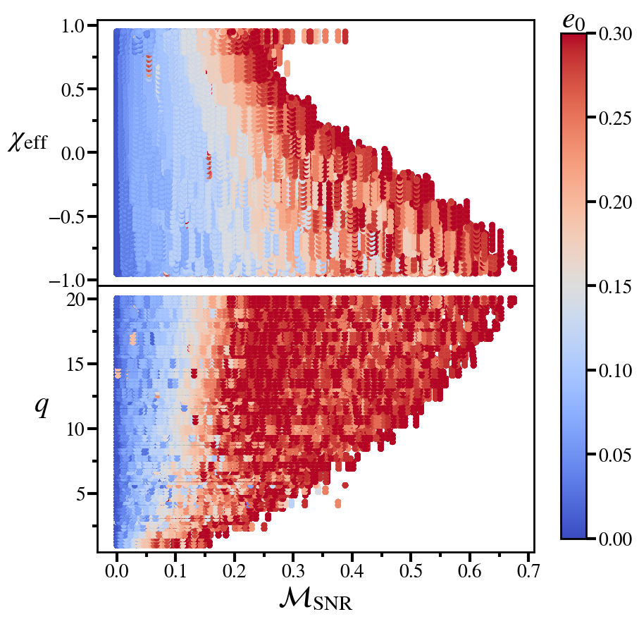
Figure 10: SNR-weighted unfaithfulness, $\mathcal{M}_{\text{SNR}}=1-\mathcal{F}_{\text{SNR}}$, averaged over the effective polarization angle and azimuthal angle of the signal for an inclination angle of the signal $\iota_{s}=\pi/3$ as described in Eq. (26), between SEOBNRv4EHM and SEOBNRv4HM in the parameter space: $q\in[1,20]$, $\chi_{1,2}\in[-0.95,0.95]$, and $e_{0}\in[0,0.3]$. The total mass considered here is $70M_{\odot}$, and the starting frequency is 20Hz. The calculations are done with the Advanced LIGO’s zero-detuned high-power design sensitivity curve Barsotti et al. (2018). In the upper panel, we show the effective spin parameter, $\chi_{\text{eff}}$, defined in Eq. (47), as a function of SNR-weighted unfaithfulness. In the lower panel, we show the same quantity as in the upper one, but using mass ratio, $q$, in the $y$-axis. The color bar indicates the value of the initial eccentricity, $e_{0}$.

IV Conclusions

Working within the EOB framework, we have developed the multipolar eccentric waveform model SEOBNRv4EHM for BBHs with non-precessing spins and multipoles $(l,|m|)=\{(2,2),(2,1),(3,3),(4,4),(5,5)\}$. The eccentric waveform model is built upon the multipolar quasi-circular SEOBNRv4HM model Bohé et al. (2017); Cotesta et al. (2018). The inspiral waveform model SEOBNRv4EHM includes recently computed eccentric corrections up to the 2PN order Khalil et al. (2021), including the spin-orbit and spin-spin interactions, in the factorized GW modes. By contrast the merger and ringdown description of the SEOBNRv4EHM model is not modified with respect to the one in the quasi-circular orbit case. Thus, we assume that the binary circularizes by the time it merges, and this is in agreement with NR simulations for mild eccentricities Hinder et al. (2008, 2018).

We have generalized the eccentric initial conditions introduced in Ref. Khalil et al. (2021) to include two eccentric parameters, the initial eccentricity $e_{0}$, and the initial relativistic anomaly $\zeta_{0}$. Both parameters are specified at a certain starting frequency $\omega_{0}$ along the elliptical orbit. We note that when the binary starts its evolution at periastron or apastron, one only needs to specify $(e_{0},\omega_{0})$, and this is the choice made in other eccentric EOB waveform models in the literature  Liu et al. (2021); Chiaramello and Nagar (2020); Nagar et al. (2021a); Nagar and Rettegno (2021); Placidi et al. (2021). The relativistic anomaly is degenerate with variations of the initial orbital frequency $\omega_{0}$ at fixed $e_{0}$. This fact is used to reduce the dimensionality of the parameter space when comparing EOB and NR waveforms in Sec. III.3. For applications like Bayesian-inference studies, having generic initial conditions becomes essential as the parameters of a binary system are inferred at a fixed reference frequency Abbott et al. (2021a). Thus, for parameter-estimation studies, the starting frequency would be fixed, and the degeneracy between $\omega_{0}$ and $\zeta_{0}$ can no longer be used to accurately sample the eccentric parameter space.

We have also implemented the initial conditions for hyperbolic encounters and dynamical-capture systems, expressing them in terms of the initial angular momentum and energy at infinity Damour et al. (2014). As an example we have shown that the SEOBNRv4EHM model can qualitatively reproduce the behavior of dynamical captures. We leave to the future a quantitative and detailed study of the accuracy of the model for hyperbolic encounters, including comparisons with NR simulations of unbound systems.

Regarding the accuracy of our model, in the quasi-circular limit we have found that the unfaithfulness between the (2,2)-mode only model, SEOBNRv4E, and the publicly available NR waveforms used to construct and validate the underlying quasi-circular waveform model, SEOBNRv4 Bohé et al. (2017), is always smaller than $1\%$. When we include the higher order multipoles, $(l,|m|)=\{(2,1),(3,3),(4,4),(5,5)\}$, the unfaithfulness averaged over sky positions, orientations and inclinations between SEOBNRv4EHM and the same NR dataset used to validate SEOBNRv4HM, is overall below $1\%$, with few configurations above that threshold, but below $1.5\%$, as in the case of SEOBNRv4HM Cotesta et al. (2018). Thus, the multipolar eccentric model has an accuracy comparable to the underlying quasi-circular model in the zero eccentricity limit.

To asses the accuracy of the model in the eccentric case, we have developed a maximization procedure of the unfaithfulness to estimate the optimal values of eccentricity and starting frequency. For the $(2,2)$-mode waveforms, we have found that the unfaithfulness of the SEOBNRv4E model against the eccentric NR waveforms at our disposal, which have eccentricity $\lesssim 0.3$, is always smaller than $1\%$. We have also used another eccentric EOB waveform model TEOBResumSE to compute the unfaithfulness against eccentric NR waveforms, and we have found that the unfaithfulness is also always $<1\%$. Overall we find that the unfaithfulness of SEOBNRv4E model is smaller than the public version of the TEOBResumSE model, at the time of this publication, for the NR dataset at our disposal. We note that in order to set more stringent constraints on the accuracy of both models, comparisons against larger datasets of eccentric NR simulations are required.

Considering that the accuracy of the SEOBNRv4EHM model against NR simulations can currently be investigated only up to eccentricity $0.3$, we have assessed the smoothness and robustness of the SEOBNRv4EHM model in the parameter space $\chi_{1,2}\in[0.,0.99]$, $q\in[1,50]$ and $e=\in[0,0.3]$. We have found that some configurations when the spins are large and positive, notably in the range $\chi_{1,2}\in[0.95,0.99]$, lead to spurious oscillations in the amplitude and frequency close to merger. This is due to the suboptimal procedure used by the SEOBNRv4EHM model to transit from the late inspiral to the merger and ringdown. Furthermore, the SEOBNRv4EHM can be generated also for eccentricity larger than $0.3$, however we caution its use for large eccentricities, especially beyond the inspiral phase, since the model has been built under the assumption that the binary circularizes. We emphasize that current GW detectors, such as LIGO, Virgo and KAGRA will be able to detect eccentric GW events with mild eccentricities  Samsing (2018); Rodriguez et al. (2018). Thus, having a waveform model that can grasp the main characteristic of eccentric signals up to eccentricity $0.3$ is valuable — for example the SEOBNRv4EHM model could be employed to search for eccentric signals in the LIGO and Virgo data and to infer the properties of the eccentric sources.

We remark that in this first eccentric EOBNR model, we have only included the eccentric corrections up to 2PN order derived in Ref. Khalil et al. (2021) to the factorized GW modes, while we have kept the conservative and dissipative dynamics the same as in the quasi-circular SEOBNRv4HM model. Preliminary comparisons with a larger set of NR simulations are indicating that better accuracy can be achieved when including the eccentric corrections Khalil et al. (2021) also in the RR forces. These improvements will be included in the next generation of the EOBNR waveform models currently under construction, that is the SEOBNRv5 model.

We leave to the near future the development of a reduced-order-model (ROM) Pürrer (2014); Yun et al. (2021) version of the SEOBNRv4EHM model, so that it can efficiently be used for inference studies on current GW catalogs and future observations with the LIGO, Virgo and KAGRA detectors. We also plan to extend the SEOBNRv4EHM model to precessing binaries, including the eccentric corrections to the waveform modes of the quasi-circular spin-precessing SEOBNRv4PHM model Pan et al. (2014); Babak et al. (2017); Ossokine et al. (2020).

Appendix A Eccentric corrections to the waveform modes

In this appendix, we list the eccentric corrections to the waveform modes obtained in Ref. Khalil et al. (2021). These corrections are written in terms of the dynamical quantities $r,p_{r}$ and $\dot{p}_{r}$. To ease the notation, we define

$$v_{\dot{\phi}}\equiv\frac{(\dot{p}_{r}r^{2}+1)^{1/6}}{\sqrt{r}},$$ (33)

which is $(\dot{\phi})^{1/3}$ at leading PN order for generic orbits, and it reduces to $v_{\omega}\equiv\omega^{1/3}$ in the circular-orbit limit. We also define the anti-symmetric mass ratio $\delta\equiv(m_{1}-m_{2})/M$ and the spin combinations

$$\chi_{S}=\frac{1}{2}(\chi_{1}+\chi_{2}),\qquad\chi_{A}=\frac{1}{2}(\chi_{1}-\chi_{2}).$$ (34)

We expand the eccentric part of the leading-order tail term, $T_{lm}^{\text{ecc}}$, in Eq. (6), in powers of the eccentricity up to $\mathcal{O}(e^{6})$, and express it in terms of the dynamical quantities $p_{r}$ and $\dot{p}_{r}$ as described in Ref. Khalil et al. (2021) using the Keplerian parametrization. For the $\{(2,2),(2,1),(3,3)\}$ modes, we obtain through 2PN order

$$T_{22}^{\text{ecc}} =-\frac{\pi}{4c^{3}r}\bigg{[}\left(4r^{3/2}\dot{p}_{r}+6ip_{r}\right)+\left(2\sqrt{r}p_{r}^{2}+ir^{2}p_{r}\dot{p}_{r}\right)+\left(\frac{5}{4}r^{5/2}p_{r}^{2}\dot{p}_{r}+\frac{1}{12}r^{11/2}\dot{p}_{r}^{3}-\frac{3}{4}ir^{4}p_{r}\dot{p}_{r}^{2}+\frac{5}{12}irp_{r}^{3}\right)$$

$$\qquad+\left(\frac{5}{4}r^{3/2}p_{r}^{4}-r^{9/2}p_{r}^{2}\dot{p}_{r}^{2}-\frac{1}{4}r^{15/2}\dot{p}_{r}^{4}+\frac{1}{8}ir^{6}p_{r}\dot{p}_{r}^{3}-\frac{15}{8}ir^{3}p_{r}^{3}\dot{p}_{r}\right)$$

$$\qquad+\left(-\frac{115}{48}r^{7/2}p_{r}^{4}\dot{p}_{r}+\frac{101}{96}r^{13/2}p_{r}^{2}\dot{p}_{r}^{3}+\frac{29}{120}r^{19/2}\dot{p}_{r}^{5}-\frac{11}{96}ir^{8}p_{r}\dot{p}_{r}^{4}+\frac{53}{24}ir^{5}p_{r}^{3}\dot{p}_{r}^{2}-\frac{589}{480}ir^{2}p_{r}^{5}\right)$$

$$\qquad+\left(-\frac{329}{480}r^{5/2}p_{r}^{6}+\frac{83}{32}r^{11/2}p_{r}^{4}\dot{p}_{r}^{2}-\frac{257}{192}r^{17/2}p_{r}^{2}\dot{p}_{r}^{4}-\frac{7}{36}r^{23/2}\dot{p}_{r}^{6}+\frac{223}{960}ir^{10}p_{r}\dot{p}_{r}^{5}-\frac{181}{72}ir^{7}p_{r}^{3}\dot{p}_{r}^{3}+\frac{111}{64}ir^{4}p_{r}^{5}\dot{p}_{r}\right)$$

$$\qquad+\mathcal{O}(p_{r},\dot{p}_{r})^{8}\bigg{]},$$ (35)

$$T_{21}^{\text{ecc}} =-\frac{\pi}{4c^{4}r}\bigg{[}8ip_{r}+\left(-r^{7/2}\dot{p}_{r}^{2}-2ir^{2}p_{r}\dot{p}_{r}+\sqrt{r}p_{r}^{2}\right)+\left(\frac{3}{2}r^{5/2}p_{r}^{2}\dot{p}_{r}+\frac{5}{6}r^{11/2}\dot{p}_{r}^{3}+\frac{2}{3}irp_{r}^{3}\right)$$

$$\qquad+\left(\frac{7}{16}r^{3/2}p_{r}^{4}-\frac{9}{4}r^{9/2}p_{r}^{2}\dot{p}_{r}^{2}-\frac{7}{16}r^{15/2}\dot{p}_{r}^{4}+\frac{5}{4}ir^{6}p_{r}\dot{p}_{r}^{3}-\frac{5}{4}ir^{3}p_{r}^{3}\dot{p}_{r}\right)$$

$$\qquad+\left(-\frac{79}{96}r^{7/2}p_{r}^{4}\dot{p}_{r}+2r^{13/2}p_{r}^{2}\dot{p}_{r}^{3}+\frac{33}{160}r^{19/2}\dot{p}_{r}^{5}-\frac{11}{8}ir^{8}p_{r}\dot{p}_{r}^{4}+\frac{19}{12}ir^{5}p_{r}^{3}\dot{p}_{r}^{2}-\frac{19}{120}ir^{2}p_{r}^{5}\right)$$

$$\qquad+\left(-\frac{59}{320}r^{5/2}p_{r}^{6}+\frac{145}{384}r^{11/2}p_{r}^{4}\dot{p}_{r}^{2}-\frac{487}{384}r^{17/2}p_{r}^{2}\dot{p}_{r}^{4}-\frac{161r^{23/2}\dot{p}_{r}^{6}}{1440}+\frac{511}{480}ir^{10}p_{r}\dot{p}_{r}^{5}-\frac{115}{144}ir^{7}p_{r}^{3}\dot{p}_{r}^{3}+\frac{61}{160}ir^{4}p_{r}^{5}\dot{p}_{r}\right)$$

$$\qquad+\mathcal{O}(p_{r},\dot{p}_{r})^{8}\bigg{]},$$ (36)

$$T_{33}^{\text{ecc}} =-\frac{\pi}{81c^{4}r}\bigg{[}\left(90r^{3/2}\dot{p}_{r}+180ip_{r}\right)+\left(-11r^{7/2}\dot{p}_{r}^{2}+22ir^{2}p_{r}\dot{p}_{r}+56\sqrt{r}p_{r}^{2}\right)+\left(2r^{5/2}p_{r}^{2}\dot{p}_{r}+\frac{331}{36}r^{11/2}\dot{p}_{r}^{3}-\frac{8}{3}ir^{4}p_{r}\dot{p}_{r}^{2}+\frac{34}{9}irp_{r}^{3}\right)$$

$$\qquad+\left(\frac{26161r^{3/2}p_{r}^{4}}{5184}+\frac{10895}{864}r^{9/2}p_{r}^{2}\dot{p}_{r}^{2}-\frac{33191r^{15/2}\dot{p}_{r}^{4}}{5184}-\frac{2383ir^{6}p_{r}\dot{p}_{r}^{3}}{1296}+\frac{14671ir^{3}p_{r}^{3}\dot{p}_{r}}{1296}\right)$$

$$\qquad+\left(\frac{3165361r^{7/2}p_{r}^{4}\dot{p}_{r}}{93312}-\frac{1286269r^{13/2}p_{r}^{2}\dot{p}_{r}^{3}}{46656}+\frac{2170663r^{19/2}\dot{p}_{r}^{5}}{466560}+\frac{17347ir^{8}p_{r}\dot{p}_{r}^{4}}{2916}-\frac{252673ir^{5}p_{r}^{3}\dot{p}_{r}^{2}}{5832}+\frac{590461ir^{2}p_{r}^{5}}{58320}\right)$$

$$\qquad+\bigg{(}\frac{269913797r^{5/2}p_{r}^{6}}{16796160}-\frac{1192721r^{11/2}p_{r}^{4}\dot{p}_{r}^{2}}{15552}+\frac{49153087r^{17/2}p_{r}^{2}\dot{p}_{r}^{4}}{1119744}-\frac{6543119r^{23/2}\dot{p}_{r}^{6}}{1679616}-\frac{10372969ir^{10}p_{r}\dot{p}_{r}^{5}}{933120}$$

$$\quad\qquad+\frac{63206059ir^{7}p_{r}^{3}\dot{p}_{r}^{3}}{839808}-\frac{27211231ir^{4}p_{r}^{5}\dot{p}_{r}}{559872}\bigg{)}+\mathcal{O}(p_{r},\dot{p}_{r})^{8}\bigg{]}.$$ (37)

For the eccentric term $f_{lm}^{\text{ecc}}$ in Eq. (6), and the modes $\{(2,2),(2,1),(3,3),(4,4),(5,5)\}$, we obtain

$$f_{22}^{\text{ecc}} =\frac{1-rp_{r}^{2}+r^{3}v_{\dot{\phi}}^{6}-2rv_{\dot{\phi}}^{2}}{2rv_{\dot{\phi}}^{2}}+irv_{\dot{\phi}}p_{r}+\frac{1}{84c^{2}r^{5}v_{\dot{\phi}}^{8}}\bigg{\{}-14(\nu+1)+ir^{2}v_{\dot{\phi}}^{3}p_{r}\left[14(\nu+1)+r^{3}v_{\dot{\phi}}^{6}\left(-101\nu+(41\nu-37)r^{3}v_{\dot{\phi}}^{6}-209\right)\right]$$

$$\qquad+r^{2}p_{r}^{4}\left[(29-10\nu)r^{3}v_{\dot{\phi}}^{6}-7(\nu-3)\right]+r^{3}v_{\dot{\phi}}^{6}\left[63\nu+r^{2}v_{\dot{\phi}}^{4}\left(-110\nu+(31\nu-8)r^{4}v_{\dot{\phi}}^{8}+(30\nu-59)rv_{\dot{\phi}}^{2}+172\right)-91\right]$$

$$\qquad+p_{r}^{2}r\left[21\nu+3r^{3}v_{\dot{\phi}}^{6}\left(3\nu+7(\nu+1)r^{3}v_{\dot{\phi}}^{6}+62\right)-7\right]+ir^{3}v_{\dot{\phi}}^{3}p_{r}^{3}\left[(41\nu-37)r^{3}v_{\dot{\phi}}^{6}-7(\nu-3)\right]\bigg{\}}$$

$$\quad+\frac{1}{6048c^{4}r^{9}v_{\dot{\phi}}^{14}}\bigg{\{}3i(103\nu^{2}-700\nu+127)r^{14}v_{\dot{\phi}}^{27}p_{r}+6r^{12}v_{\dot{\phi}}^{24}\left[318-4\nu(96\nu+265)+(40\nu^{2}+20\nu-71)rp_{r}^{2}\right]$$

$$\qquad+6ir^{11}v_{\dot{\phi}}^{21}p_{r}\left[80+1531\nu-640\nu^{2}+(349-143\nu^{2}-724\nu)rp_{r}^{2}\right]+24(55\nu-86)r^{8}v_{\dot{\phi}}^{16}\left[1-\nu+(\nu+1)rp_{r}^{2}\right]$$

$$\qquad+6r^{9}v_{\dot{\phi}}^{18}\left[-616+955\nu-409\nu^{2}+(17\nu^{2}+193\nu-340)r^{2}p_{r}^{4}-(1181\nu^{2}+1277\nu+279)rp_{r}^{2}\right]$$

$$\qquad-105ir^{2}v_{\dot{\phi}}^{3}p_{r}\left[(\nu-3)rp_{r}^{2}-2(\nu+1)\right]^{2}+24(55\nu-86)r^{5}v_{\dot{\phi}}^{10}\left[(\nu-3)rp_{r}^{2}-2(\nu+1)\right]$$

$$\qquad+ir^{8}v_{\dot{\phi}}^{15}p_{r}\left[13\nu(3598-517\nu)-3(389\nu^{2}+748\nu-571)r^{2}p_{r}^{4}+12(281\nu^{2}-349\nu+803)rp_{r}^{2}-9221\right]$$

$$\qquad+6ir^{5}v_{\dot{\phi}}^{9}p_{r}\left[50\nu^{2}-872\nu+(22\nu^{2}+55\nu-216)r^{2}p_{r}^{4}-(69\nu^{2}+674\nu+953)rp_{r}^{2}-166\right]$$

$$\qquad+6r^{3}v_{\dot{\phi}}^{6}\left[28(17\nu-16\nu^{2}+6)+(43\nu^{2}+13\nu-279)r^{3}p_{r}^{6}-(243\nu^{2}+325\nu+1253)r^{2}p_{r}^{4}+2(269\nu^{2}-446\nu+237)rp_{r}^{2}\right]$$

$$\qquad+6r^{6}v_{\dot{\phi}}^{12}\left[2\nu(733\nu-620)+(80\nu^{2}+130\nu-277)r^{3}p_{r}^{6}+\left(-294\nu^{2}+380\nu-1963\right)r^{2}p_{r}^{4}-2(205\nu^{2}+2604\nu+93)rp_{r}^{2}+26\right]$$

$$\qquad-168\left(rp_{r}^{2}-1\right)\left[(\nu-3)rp_{r}^{2}-2(\nu+1)\right]^{2}+6(103\nu^{2}-43\nu-8)r^{15}v_{\dot{\phi}}^{30}+24(\nu+1)(55\nu-86)r^{11}v_{\dot{\phi}}^{22}\bigg{\}}$$

$$\quad+\frac{1}{6c^{3}r^{4}v_{\dot{\phi}}^{5}}\bigg{\{}\chi_{S}\left[2-\nu+i(5\nu-8)r^{2}v_{\dot{\phi}}^{3}p_{r}+(\nu-2)rp_{r}^{2}+r^{3}v_{\dot{\phi}}^{6}\left(9\nu-8(\nu-1)rv_{\dot{\phi}}^{2}-10\right)\right]$$

$$\qquad-2\delta\chi_{A}\left[-1+4ir^{2}v_{\dot{\phi}}^{3}p_{r}+rp_{r}^{2}+r^{3}v_{\dot{\phi}}^{6}\left(5-4rv_{\dot{\phi}}^{2}\right)\right]\bigg{\}}$$

$$\quad+\frac{1}{6c^{4}r^{6}v_{\dot{\phi}}^{8}}\bigg{\{}2\delta\chi_{A}\chi_{S}\bigg{[}i(2\nu-1)r^{3}v_{\dot{\phi}}^{3}p_{r}^{3}+rp_{r}^{2}\left(\nu+5(2\nu-1)r^{3}v_{\dot{\phi}}^{6}+1\right)+(2\nu-1)r^{2}p_{r}^{4}-3ip_{r}\left(2(2\nu-1)r^{5}v_{\dot{\phi}}^{9}-\nu r^{2}v_{\dot{\phi}}^{3}\right)$$

$$\quad\qquad-3\left(r^{3}v_{\dot{\phi}}^{6}-1\right)\left((2\nu+1)r^{3}v_{\dot{\phi}}^{6}-\nu\right)\bigg{]}+\chi_{S}^{2}\bigg{[}rp_{r}^{2}\left(-2\nu^{2}+2\nu-5(1-2\nu)^{2}r^{3}v_{\dot{\phi}}^{6}+1\right)-i(1-2\nu)^{2}r^{3}v_{\dot{\phi}}^{3}p_{r}^{3}-(1-2\nu)^{2}r^{2}p_{r}^{4}$$

$$\quad\qquad+6ip_{r}\left((1-2\nu)^{2}r^{5}v_{\dot{\phi}}^{9}-(\nu-1)\nu r^{2}v_{\dot{\phi}}^{3}\right)+3\left(r^{3}v_{\dot{\phi}}^{6}-1\right)\left((4\nu^{2}-4\nu-1)r^{3}v_{\dot{\phi}}^{6}-2(\nu-1)\nu\right)\bigg{]}$$

$$\qquad+\chi_{A}^{2}(4\nu-1)r\left[-6ir^{4}v_{\dot{\phi}}^{9}p_{r}+p_{r}^{2}\left(5r^{3}v_{\dot{\phi}}^{6}-1\right)+ir^{2}v_{\dot{\phi}}^{3}p_{r}^{3}+rp_{r}^{4}+3r^{2}v_{\dot{\phi}}^{6}\left(r^{3}v_{\dot{\phi}}^{6}-1\right)\right]\bigg{\}}+\mathcal{O}\left(\frac{1}{c^{5}}\right),$$ (38)

$$f_{21}^{\text{ecc}} =\frac{1-r^{2}v_{\dot{\phi}}^{4}}{r^{2}v_{\dot{\phi}}^{4}}-\frac{1}{42c^{2}r^{6}v_{\dot{\phi}}^{10}}\left\{28(\nu+1)+3i(12\nu-83)r^{5}v_{\dot{\phi}}^{9}p_{r}+r^{3}v_{\dot{\phi}}^{6}\left(82-52\nu+(19\nu+106)rp_{r}^{2}\right)-14(\nu-3)rp_{r}^{2}+2(12\nu-55)r^{6}v_{\dot{\phi}}^{12}\right\}$$

$$\quad+\frac{1}{4c\delta r^{4}v_{\dot{\phi}}^{7}}\left[\chi_{A}\left(6r^{4}v_{\dot{\phi}}^{8}-6\right)+6\delta\left(r^{4}v_{\dot{\phi}}^{8}-1\right)\chi_{S}\right]+\frac{1}{336c^{3}\delta r^{8}v_{\dot{\phi}}^{13}}\bigg{\{}\chi_{A}\bigg{[}588(\nu+1)+24i(104\nu-147)r^{5}v_{\dot{\phi}}^{9}p_{r}+42(\nu-1)r^{7}v_{\dot{\phi}}^{14}$$

$$\quad\qquad-6p_{r}^{2}\left(7(\nu+1)r^{8}v_{\dot{\phi}}^{14}+7(\nu-3)r^{5}v_{\dot{\phi}}^{8}-(141\nu+203)r^{4}v_{\dot{\phi}}^{6}+49(\nu-3)r\right)-42(\nu+1)r^{10}v_{\dot{\phi}}^{20}-4(131\nu+427)r^{8}v_{\dot{\phi}}^{16}$$

$$\quad\qquad+30(121\nu-35)r^{6}v_{\dot{\phi}}^{12}+84(\nu+1)r^{4}v_{\dot{\phi}}^{8}+2(1085-1889\nu)r^{3}v_{\dot{\phi}}^{6}\bigg{]}-2\delta\chi_{S}\bigg{[}-294(\nu+1)+36i(2\nu+49)r^{5}v_{\dot{\phi}}^{9}p_{r}$$

$$\quad\qquad+3p_{r}^{2}\left(7(\nu+1)r^{8}v_{\dot{\phi}}^{14}+7(\nu-3)r^{5}v_{\dot{\phi}}^{8}-(69\nu+203)r^{4}v_{\dot{\phi}}^{6}+49(\nu-3)r\right)+21(\nu+1)r^{10}v_{\dot{\phi}}^{20}+2(79\nu+427)r^{8}v_{\dot{\phi}}^{16}$$

$$\quad\qquad-21(\nu-1)r^{7}v_{\dot{\phi}}^{14}+15(35-33\nu)r^{6}v_{\dot{\phi}}^{12}-42(\nu+1)r^{4}v_{\dot{\phi}}^{8}+(673\nu-1085)r^{3}v_{\dot{\phi}}^{6}\bigg{]}\bigg{\}}+\mathcal{O}\left(\frac{1}{c^{4}}\right),$$ (39)

$$f_{33}^{\text{ecc}} =\frac{2}{9rv_{\dot{\phi}}^{3}}\left[3ir^{3}v_{\dot{\phi}}^{6}p_{r}-3r^{2}v_{\dot{\phi}}^{3}p_{r}^{2}-irp_{r}^{3}+2ip_{r}+r^{4}v_{\dot{\phi}}^{9}-rv_{\dot{\phi}}^{3}\right]+\frac{1}{162c^{2}r^{5}v_{\dot{\phi}}^{9}}\bigg{\{}-36(\nu-2)r^{6}v_{\dot{\phi}}^{9}p_{r}^{4}+6r^{5}v_{\dot{\phi}}^{9}p_{r}^{2}\left[18\nu-(\nu-11)r^{3}v_{\dot{\phi}}^{6}+57\right]$$

$$\qquad+6irp_{r}^{3}\left[6(\nu-1)+r^{3}v_{\dot{\phi}}^{6}\left(-4\nu+2(5\nu-1)r^{3}v_{\dot{\phi}}^{6}+35\right)\right]+3r^{4}v_{\dot{\phi}}^{9}\left[56\nu+r^{3}v_{\dot{\phi}}^{6}\left(42\nu+2(5\nu-1)r^{3}v_{\dot{\phi}}^{6}-39\right)+27(7-4\nu)rv_{\dot{\phi}}^{2}-148\right]$$

$$\qquad+ip_{r}\left[r^{3}v_{\dot{\phi}}^{6}\left(100\nu+9r^{3}v_{\dot{\phi}}^{6}\left(-23\nu+(7\nu-5)r^{3}v_{\dot{\phi}}^{6}-29\right)-218\right)-36(\nu+1)\right]-3ir^{2}p_{r}^{5}\left[3(\nu-3)+(\nu-11)r^{3}v_{\dot{\phi}}^{6}\right]\bigg{\}}$$

$$\quad\frac{1}{18c^{3}\delta r^{4}v_{\dot{\phi}}^{6}}\bigg{\{}\chi_{A}\left[2ip_{r}\left(-16\nu+(101\nu-24)r^{3}v_{\dot{\phi}}^{6}+4\right)+2(6-25\nu)r^{2}v_{\dot{\phi}}^{3}p_{r}^{2}+4i(4\nu-1)rp_{r}^{3}-4(5\nu-1)rv_{\dot{\phi}}^{3}\left(r^{3}v_{\dot{\phi}}^{6}-1\right)\right]$$

$$\qquad+2\delta\chi_{S}\left[ip_{r}\left(-2\nu+(17\nu-24)r^{3}v_{\dot{\phi}}^{6}+4\right)+2(3-2\nu)r^{2}v_{\dot{\phi}}^{3}p_{r}^{2}+i(\nu-2)rp_{r}^{3}-(3\nu-2)rv_{\dot{\phi}}^{3}\left(r^{3}v_{\dot{\phi}}^{6}-1\right)\right]\bigg{\}}+\mathcal{O}\left(\frac{1}{c^{4}}\right),$$ (40)

$$f_{44}^{\text{ecc}} =\frac{1}{64r^{2}v_{\dot{\phi}}^{4}}\left\{7+r\left[24ir^{4}v_{\dot{\phi}}^{9}p_{r}+3r^{2}v_{\dot{\phi}}^{6}\left(17-12rp_{r}^{2}\right)-6irv_{\dot{\phi}}^{3}p_{r}\left(4rp_{r}^{2}-9\right)+6p_{r}^{2}\left(rp_{r}^{2}-3\right)+6r^{5}v_{\dot{\phi}}^{12}-64rv_{\dot{\phi}}^{4}\right]\right\}$$

$$\quad+\frac{1}{42240(3\nu-1)c^{2}r^{6}v_{\dot{\phi}}^{10}}\bigg{\{}-3r^{9}v_{\dot{\phi}}^{18}\left[60\nu(889-636\nu)+20(\nu(321\nu-926)+238)rp_{r}^{2}-10481\right]$$

$$\qquad+120i(267\nu^{2}-278\nu+49)r^{11}v_{\dot{\phi}}^{21}p_{r}+6ir^{8}v_{\dot{\phi}}^{15}p_{r}\left[8033-5\nu(4551\nu+3622)+1320(\nu+1)(3\nu-1)rp_{r}^{2}\right]$$

$$\qquad+r^{6}v_{\dot{\phi}}^{12}\left[-780\nu(234\nu-289)-60(519\nu^{2}-794\nu+172)r^{2}p_{r}^{4}+6(10\nu(2265\nu+1882)-9847)rp_{r}^{2}-46063\right]$$

$$\qquad-6ir^{5}v_{\dot{\phi}}^{9}p_{r}\left[5\nu(12748-2727\nu)+20(69\nu^{2}-410\nu+115)r^{2}p_{r}^{4}+(10277-5\nu(525\nu+5294))rp_{r}^{2}-20789\right]$$

$$\qquad+20r^{3}v_{\dot{\phi}}^{6}\left[3315\nu^{2}-2644\nu-3(15\nu^{2}+238\nu-74)r^{3}p_{r}^{6}+3(339\nu^{2}-1274\nu+422)r^{2}p_{r}^{4}-2(1797\nu^{2}-4910\nu+1510)rp_{r}^{2}+553\right]$$

$$\qquad-330i(3\nu-1)r^{2}v_{\dot{\phi}}^{3}p_{r}\left(4rp_{r}^{2}-9\right)\left[(\nu-3)rp_{r}^{2}-2(\nu+1)\right]+220(3\nu-1)\left[6r\left(rp_{r}^{2}-3\right)p_{r}^{2}+7\right]\left[(\nu-3)rp_{r}^{2}-2(\nu+1)\right]$$

$$\qquad+60(183\nu^{2}-106\nu+8)r^{12}v_{\dot{\phi}}^{24}\bigg{\}}+\mathcal{O}\left(\frac{1}{c^{3}}\right),$$ (41)

$$f_{55}^{\text{ecc}} =\frac{1}{625r^{2}v_{\dot{\phi}}^{5}}\bigg{\{}120ir^{6}v_{\dot{\phi}}^{12}p_{r}+3r^{4}v_{\dot{\phi}}^{9}\left(143-80rp_{r}^{2}\right)-48ir^{3}v_{\dot{\phi}}^{6}p_{r}\left(5rp_{r}^{2}-13\right)+4rv_{\dot{\phi}}^{3}\left(30r^{2}p_{r}^{4}-99rp_{r}^{2}+43\right)+24r^{7}v_{\dot{\phi}}^{15}-625r^{2}v_{\dot{\phi}}^{5}$$

$$\qquad+2ip_{r}\left[12r\left(rp_{r}^{2}-4\right)p_{r}^{2}+41\right]\bigg{\}}+\mathcal{O}\left(\frac{1}{c}\right).$$ (42)

For binaries of equal masses ($\delta=0,\,\nu=1/4$), the leading-PN order of the odd-$m$ modes is proportional to $\delta$, which cancels with the denominator of $\chi_{A}/\delta$ in the above expressions for the $(2,1)$ and $(3,3)$ modes, leading to

$$f_{21}^{\text{ecc},\delta=0} =\frac{3\chi_{A}}{2cv_{\dot{\phi}}^{7}}\left(v_{\dot{\phi}}^{8}-\frac{1}{r^{4}}\right)$$

$$+\frac{\chi_{A}}{224c^{3}r^{8}v_{\dot{\phi}}^{13}}\bigg{[}rp_{r}^{2}\left(35r^{7}v_{\dot{\phi}}^{14}-77r^{4}v_{\dot{\phi}}^{8}-953r^{3}v_{\dot{\phi}}^{6}-539\right)$$

$$\quad+1936ir^{5}v_{\dot{\phi}}^{9}p_{r}+35r^{10}v_{\dot{\phi}}^{20}+1226r^{8}v_{\dot{\phi}}^{16}+21r^{7}v_{\dot{\phi}}^{14}$$

$$\quad+95r^{6}v_{\dot{\phi}}^{12}-70r^{4}v_{\dot{\phi}}^{8}-817r^{3}v_{\dot{\phi}}^{6}-490\bigg{]},$$ (43)

$$f_{33}^{\text{ecc},\delta=0} =\frac{\chi_{A}}{36c^{3}r^{3}v_{\dot{\phi}}^{3}}\left[2-r\left(-5irv_{\dot{\phi}}^{3}p_{r}+p_{r}^{2}+2r^{2}v_{\dot{\phi}}^{6}\right)\right].$$ (44)

Since the eccentric correction to the $(5,5)$-mode does not depend on spin at this order, it goes to zero for equal masses.

Appendix B Implementation of the orbit averaging procedure

In this appendix, we describe in detail the orbit averaging procedure that we have applied in Sec. II.2 to the instantaneous NQC functions of the waveform.

According to Eq. (9), to orbit average a dynamical quantity we need to define the times, $t_{i}$, which identify successive orbits in the evolution. In our implementation, we use the local maxima and employ a simple algorithm that compares each element of the time series with the two closest neighbors. However, these values may strongly depend on the specified time step, thus, in order to reduce such dependence we further compute the parabola passing through these three points $\{(t_{i-1},X_{i-1}),(t_{i},X_{i}),(t_{i+1},X_{i+1})\}$, and obtain its maxima analytically,

$$\begin{split}f(t)&=at^{2}+bt+c,\quad t_{\text{max}}=-b/2a,\\ \Delta&=(t_{i}-t_{i+1})(t_{i}-t_{i-1})(t_{i+1}-t_{i-1})\\ a&=\frac{1}{\Delta}\left[X_{i-1}(t_{i}-t_{i+1})+X_{i}(t_{i+1}-t_{i-1})+X_{i+1}(-t_{i}+t_{i-1}))\right],\\ b&=\frac{1}{\Delta}\left[X_{i-1}(-t_{i}^{2}+t_{i+1}^{2})+X_{i+1}(t_{i}^{2}-t_{i-1}^{2})+X_{i}(-t_{i+1}^{2}+t_{i-1}^{2})\right],\\ c&=\frac{1}{\Delta}\left[(X_{i-1}(t_{i}-t_{i+1})t_{i}t_{i+1}+X_{i}(t_{i+1}-t_{i-1})t_{i-1}t_{i+1}\right.\\ &\left.+X_{i+1}t_{i}t_{i-1}(-t_{i}+t_{i-1}))\right],\end{split}$$ (45)

where $t_{\text{max}}$ is the solution of $df(t)/dt=0$. The found maxima, and their corresponding times, $\{t_{i},X_{i}\}$, are then used in Eq. (9) to compute the orbit-average quantity $\overline{X}_{i}$, and the intermediate times, $\overline{t}_{i}=(t_{i+1}+t_{i})/2$ Lewis et al. (2017), are associated to each $\overline{X}_{i}$.

As our dynamical quantity, we use $p_{r_{*}}$, but when the eccentricity $e_{0}<0.1$, we switch to $\dot{p}_{r*}$, because we find that we can reliably extract the maxima in this quantity even for very small eccentricities ($e_{0}<0.01$). This is due to the fact that the time derivative enhances the effects of the eccentric oscillations.

The orbit averaging procedure also requires the introduction of boundary conditions at the start and at the end of the inspiral . At the start of the inspiral, we simply use the the time of the first maximum, $t^{\text{first-max}}$. The impact of this choice is negligible because at this point of the evolution the orbit-average NQC function is quite smooth. Meanwhile, at the end of the inspiral, we need to reproduce the plunging behavior of the dynamical quantities $r,\omega,p_{r_{*}}$ to accurately compute the NQC function, as done in the quasi-circular case. To achieve this goal, we impose that from a certain time, $t^{\text{average-end}}$, the orbit-average dynamical quantities follow the non-orbit–average dynamics. In Fig. 11, we show how the orbit-average $\omega$ and $p_{r_{*}}$ are constructed from the instantaneous eccentric dynamics for a particular eccentric configuration, $q=3,\quad\chi_{1}=0.5,\quad\chi_{2}=0.25,\quad e_{0}=0.3$. Additionally, the evolution of the quasi-circular quantities is included in Fig. 11, showing that the orbit-average curves for $\omega$ and $p_{r_{*}}$ agree remarkably well with the ones corresponding to the quasi-circular evolution.

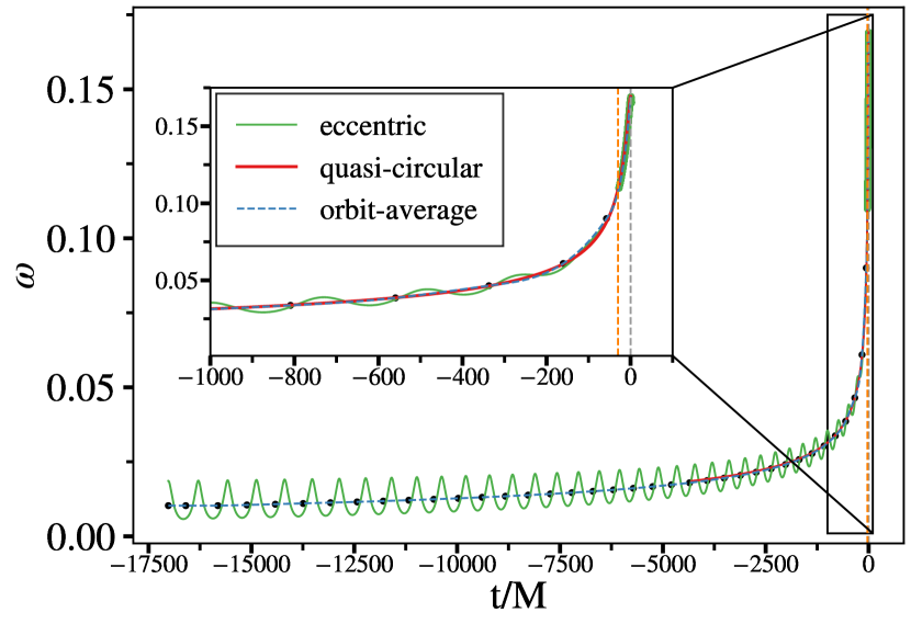
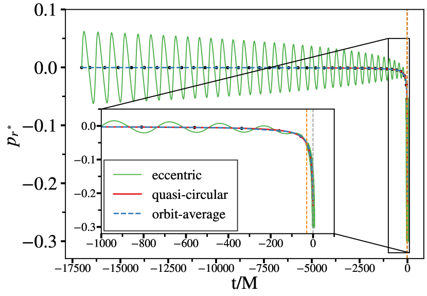
Figure 11: Time evolution of the orbital frequency $\omega$ (upper panel), and the radial momentum $p_{r*}$ (lower panel), for a configuration with $q=3$, $\chi_{1}=0.5$, $\chi_{2}=0.25$. For this configuration, we show the quasi-circular dynamical quantities (red solid line), the eccentric quantities with initial eccentricity $e_{0}=0.3$ (solid green line) and the orbit-average curves (blue dashed line). The black dots, on the left of the orange vertical line, represent the $\{\overline{t}_{i},\overline{X}_{i}\}$ points used to construct the orbit-average curve, the orange vertical line represents the time $t^{\text{average-end}}=-30M$ from which the instantaneous quantities are used to construct the orbit-average curve, and the gray vertical line corresponds to time at which the inspiral ends, that is $t^{\text{inspiral-end}}$. The green dots, on the right of the vertical orange line, corresponds to values of the instantaneous eccentric quantities, which are used together with the black dots to generate the interpolated function representing the orbit-average curve. The insets in both panels zoom into the last $1000M$ of evolution to better show the behavior of the orbit average curves at the end of the inspiral.

In Fig. 11, the orange vertical line corresponds to $t^{\text{average-end}}$, from which the values of the instantaneous, eccentric dynamical variables (green dots on the right of the orange vertical line) are attached, and together with the orbit-average values (black dots on the left of the orange vertical line) form the orbit-average curve, which is then interpolated. Thus, between the time of the last found maximum, $t^{\text{last-max}}$ (the closest black dot to the orange vertical line), and the value of $t^{\text{average-end}}$ there are no points to use. If the distance between $t^{\text{last-max}}$ and $t^{\text{average-end}}$ is too large, one can get unphysical oscillations coming from interpolation artefacts due to a too large interpolated interval without points. By contrast if $t^{\text{average-end}}$ is very close to $t^{\text{last-max}}$ one could introduce residual oscillations due to eccentricity, or spurious oscillations due to the artefacts of the interpolation method, as at plunge the change of behavior of the dynamical quantities, especially $p_{r^{*}}$, challenges the interpolation procedure. Furthermore, we note that the position of $t^{\text{last-max}}$ depends substantially on the spins of the binary. For instance, for high-negative spins $t^{\text{last-max}}$ typically occurs far from the merger ($t^{\omega_{\text{peak}}}-t^{\text{last-max}}\gtrsim 100M$), while for high-positive spins $t^{\text{last-min}}$ can be very close to merger $t^{\omega_{\text{peak}}}-t^{\text{last-max}}\lesssim 50M$. We use the following phenomenological prescription for the dependence of $t^{\text{average-end}}$ with spins,

$$\begin{split}&t_{\chi}^{\text{average-end}}(t_{j}^{\text{average-end}},\chi_{\text{low}},\chi_{\text{high}},\beta_{\chi};\chi_{\text{eff}})=\\ &\quad\qquad t^{\text{average-end}}_{0}\times\left[1-w(\beta_{\chi},\chi_{\text{low}};\chi_{\text{eff}})\right]\\ &\qquad+t^{\text{average-end}}_{1}\times\left[1-w(\beta_{\chi},\chi_{\text{high}};\chi_{\text{eff}})\right]\\ &\qquad+t_{2}^{\text{average-end}}\times w(\beta_{\chi},\chi_{\text{high}};\chi_{\text{eff}}),\end{split}$$ (46)

where the function $w$ is the sigmoid defined in Eq. (8), and, the effective spin parameter is defined as,

$$\chi_{\text{eff}}=\frac{m_{1}\chi_{1}+m_{2}\chi_{2}}{M}.$$ (47)

In Eq. (46) the indices takes the values $j=0,1,2$, while $\beta_{\chi}=50$, $\{\chi_{\text{low}},\chi_{\text{high}}\}=\{-0.5,0.95\}$ and $(t^{\text{average-end}}_{0},t^{\text{average-end}}_{1},t^{\text{average-end}}_{2})=(60M,30M,20M)$. In Fig. 12 the dependence of $t^{\chi}_{\text{average-end}}$ on the effective spin parameter is illustrated. The values of the parameters $\{t^{\text{average-end}}_{0},t^{\text{average-end}}_{1},t^{\text{average-end}}_{2},\chi_{\text{low}},\chi_{\text{high}}\}$ are chosen after evaluating the model in a grid of points in parameter space $q=[1-20]$, $\chi_{\text{eff}}=[-0.99,0.99]$, $e=[0,0.3]$ with $t_{\text{append}}=[10,100]$, and imposing that the frequency of the (2,2)-mode does not have oscillations above $20\%$ with respect to the (2,2)-mode frequency of the quasi-circular SEOBNRv4 model in the last 100M prior to the peak of the (2,2)-mode amplitude. We note that the current prescription for the $t^{\text{average-end}}$ parameter is independent of the mass ratio, because we find that the spin effects are dominant for the mass ratios we consider here.

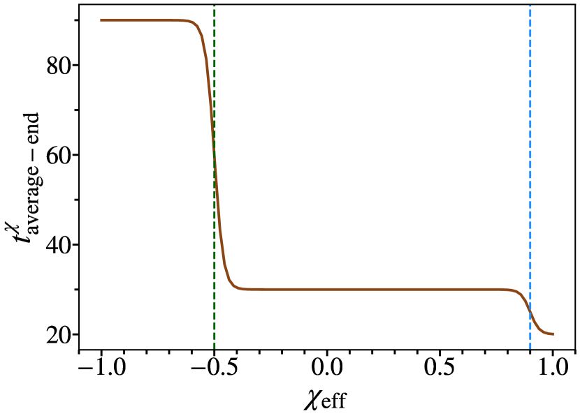
Figure 12: Dependence of the $t_{\chi}^{\text{average-end}}$ parameter defined in Eq. (47) on the effective spin parameter. The green (blue) dashed vertical line corresponds to $\chi_{\text{low}}=-0.5$ ($\chi_{\text{high}}=0.95)$ values used to construct $t_{\chi}^{\text{average-end}}$.

We note that the orbit averaging procedure fails when eccentricity goes to zero due to the absence of maxima in the orbital quantities, as they become non-oscillatory functions. Hence, in order to have a smooth transition to the quasi-circular limit, we need a new metric to measure the distance between the time of the last found maxima, $t^{\text{last-max}}$, and the time corresponding to $t^{\text{average-end}}_{\chi}$. This is due to the fact that the smaller the eccentricity, the earlier $t^{\text{last-max}}$ occurs in the inspiral, and thus, the larger the region without points over which the orbit-average quantities would be interpolated. In practice, we find that one can use the time at which the inspiral ends, $t^{\text{inspiral-end}}$ (dashed gray vertical line in Fig. 11), instead of $t^{\text{average-end}}_{\chi}$, because for low eccentricities a difference of $\sim 30-100M$ has negligible impact in the orbit averaging procedure. Hence, we impose that $t^{\text{average-end}}$ depends on

$$\begin{split}\Delta t=t^{\text{inspiral-end}}-t^{\text{last-max}},\end{split}$$ (48)

such that the final expression for the $t^{\text{average-end}}$ reads as follows,

$$\begin{split}t^{\text{average-end}}(\Delta t,\chi_{\text{eff}})&=t_{\chi}^{\text{average-end}}(\chi_{\text{eff}})\times[1-w(\beta_{t},\Delta t_{0};\Delta t)]\\ &+\alpha_{t}\times w(\beta_{t},\Delta t_{0};\Delta t)\times\Delta t,\end{split}$$ (49)

where $\beta_{t}=0.1$, $\Delta t_{0}=350M$ and $\alpha_{t}=0.75$. This choice of parameters ensures that $t^{\text{average-end}}$ increases as the time at which the last maximum is found occurs at earlier times in the inspiral for low-initial eccentricities, thus smoothly increasing the region in which the instantaneous variables are used to construct the orbit-average quantities. These values were set after testing and evaluating more than $10^{4}$ waveforms for initial eccentricities $e<0.1$ in the parameter space $q=[1,20]$, $\chi_{\text{eff}}=[-0.9,0.9]$. Finally, we only consider the orbit averaging procedure when at least three maxima are found during the inspiral, otherwise we use the instantaneous dynamics to construct the NQC function in Eq. (7).

Appendix C PN expressions for dynamical quantities in the Keplerian parametrization

In this appendix, we provide the expressions of the dynamical quantities $p_{r},\dot{p}_{r},$ and $\dot{r}$ in the Keplerian parametrization. They are needed for calculating the initial conditions for eccentric orbits, as discussed in Sec. II.3.

In the Keplerian parametrization we have:

$$r=\frac{1}{u_{p}(1+e\cos\zeta)}\,,$$ (50)

where $u_{p}$ is the inverse semilatus rectum and $\zeta$ is the relativistic anomaly. Inverting the Hamiltonian at periastron and apastron, $r_{\pm}=[u_{p}(1\pm e)]^{-1}$, and solving for the energy $E$ and $u_{p}$ through to 2PN order, we obtain

$$E =\frac{e^{2}-1}{2p_{\phi}^{2}}+\frac{1-e^{2}}{8c^{2}p_{\phi}^{4}}\left[e^{2}(\nu-7)-\nu-9\right]+\frac{e^{2}-1}{16c^{4}p_{\phi}^{6}}\left[e^{4}(\nu^{2}-7\nu+33)-2e^{2}(\nu^{2}+9\nu-71)+(\nu-7)\nu+81\right]$$

$$\quad+\frac{1-e^{4}}{c^{3}p_{\phi}^{5}}\left[2\delta\chi_{A}-(\nu-2)\chi_{S}\right]+\frac{1-e^{2}}{2c^{4}L^{6}}\left\{\chi_{S}^{2}\left[e^{2}\left(-8\nu^{2}+8\nu-3\right)-1\right]+\chi_{A}^{2}\left(3e^{2}+1\right)(4\nu-1)+2\delta\chi_{A}\chi_{S}\left[e^{2}(4\nu-3)-1\right]\right\},$$

$$u_{p} =\frac{1}{p_{\phi}^{2}}+\frac{e^{2}+3}{c^{2}p_{\phi}^{4}}+\frac{e^{2}+3}{c^{4}p_{\phi}^{6}}\left(2e^{2}-\nu+6\right)+\frac{e^{2}+3}{c^{3}p_{\phi}^{5}}\left[-2\delta\chi_{A}+(\nu-2)\chi_{S}\right]$$

$$\quad+\frac{2}{c^{4}p_{\phi}^{6}}\left\{\chi_{S}^{2}\left[e^{2}\left(3\nu^{2}-3\nu+1\right)+\nu^{2}-\nu+1\right]-\chi_{A}^{2}\left(e^{2}+1\right)(4\nu-1)-\delta\chi_{A}\chi_{S}\left[e^{2}(3\nu-2)+\nu-2\right]\right\}.$$ (51)

Inverting the Hamiltonian to obtain $p_{r}(E,p_{\phi},r)$, then substituting Eqs. (50) and (C), yields $p_{r}(p_{\phi},e,\zeta)$, which is given by the 2PN expansion

$$p_{r} =\frac{e\sin\zeta}{p_{\phi}}+\frac{e\sin\zeta}{c^{2}p_{\phi}^{3}}\left(e^{2}+e\cos\zeta+2\right)+\frac{e^{2}\sin\zeta(e-\cos\zeta)\left[-2\delta\chi_{A}+(\nu-2)\chi_{S}\right]}{c^{3}p_{\phi}^{4}}+\frac{e\sin\zeta}{4c^{4}p_{\phi}^{5}}\bigg{\{}8e^{4}+e^{2}(43-10\nu)-12\nu+22$$

$$\quad+\left[8e^{3}+e(12-20\nu)\right]\cos\zeta+e^{2}(3-6\nu)\cos(2\zeta)+\chi_{A}^{2}\left[e^{2}(8\nu-2)\cos(2\zeta)+e^{2}(4-16\nu)+e(48\nu-12)\cos\zeta+24\nu-6\right]$$

$$\quad+\chi_{S}^{2}\left[-2e^{2}(1-2\nu)^{2}\cos(2\zeta)+e^{2}(8(\nu-1)\nu+4)+e(-40(\nu-1)\nu-12)\cos\zeta-6(1-2\nu)^{2}\right]$$

$$\quad-\delta\chi_{A}\chi_{S}\left[e^{2}(4-8\nu)\cos(2\zeta)+8e^{2}(\nu-1)+e(24-40\nu)\cos\zeta-24\nu+12\right]\bigg{\}}.$$ (52)

Substituting $r$ and $p_{r}$ from Eqs. (50) and (C) into $\dot{p}_{r}=-\partial\hat{H}_{\text{EOB}}/\partial r$, and expanding yields

$$\dot{p}_{r} =\frac{e\cos\zeta(e\cos\zeta+1)^{2}}{p_{\phi}^{4}}-\frac{e(e\cos\zeta+1)^{2}\left[\left(e^{2}(\nu-5)-\nu-7\right)\cos\zeta+e(\cos(2\zeta)+3)\right]}{2c^{2}p_{\phi}^{6}}+\frac{e(e\cos\zeta+1)^{2}\left[-2\delta\chi_{A}+(\nu-2)\chi_{S}\right]}{2c^{3}p_{\phi}^{7}}$$

$$\qquad\times\left[6\left(e^{2}+1\right)\cos\zeta-e(3\cos(2\zeta)+1)\right]+\frac{e(e\cos\zeta+1)^{2}}{8c^{4}p_{\phi}^{8}}\bigg{\{}2e\left[\left(e^{2}(\nu-7)-7\nu-41\right)\cos(2\zeta)+3e^{2}(\nu-7)-6e\nu\cos(3\zeta)+11\nu-59\right]$$

$$\qquad+\left[e^{4}(3\nu^{2}-17\nu+55)-6e^{2}(\nu^{2}+3\nu-39)+3\nu^{2}-\nu+95\right]\cos\zeta\bigg{\}}$$

$$\quad+\frac{e(e\cos\zeta+1)^{2}}{4c^{4}p_{\phi}^{8}}\bigg{\{}2\delta\chi_{A}\chi_{S}\left[\left(e^{2}(19-26\nu)+12\nu\right)\cos(\zeta)+3e^{2}(2\nu-1)\cos(3\zeta)+2e(11\nu-7)\cos(2\zeta)+2e(\nu-1)\right]$$

$$\qquad+\chi_{S}^{2}\left[\left(e^{2}\left(52\nu^{2}-52\nu+19\right)-24(\nu-1)\nu\right)\cos(\zeta)-e\left(3e(1-2\nu)^{2}\cos(3\zeta)+2\left(22\nu^{2}-22\nu+7\right)\cos(2\zeta)+4\nu^{2}-4\nu+2\right)\right]$$

$$\qquad+\chi_{A}^{2}e(4\nu-1)[-19e\cos\zeta+3e\cos(3\zeta)+14\cos(2\zeta)+2]\bigg{\}}.$$ (53)

Similarly, for $\dot{r}=\partial\hat{H}_{\text{EOB}}/\partial p_{r}$, we obtain

$$\dot{r} =\frac{e\sin\zeta}{p_{\phi}}+\frac{e\sin\zeta}{2c^{2}p_{\phi}^{3}}\left[e^{2}(-(\nu-1))-6e\cos\zeta+\nu-3\right]+\frac{e^{2}\sin\zeta(\cos\zeta-e)}{c^{3}p_{\phi}^{4}}\left[2\delta\chi_{A}+(2-\nu)\chi_{S}\right]$$

$$\quad+\frac{e}{8c^{4}p_{\phi}^{5}}\left\{2e\left(3e^{2}(\nu-3)+11\nu-29\right)\sin(2\zeta)+3e^{2}(2\nu+1)\sin(3\zeta)+\left[e^{4}(3(\nu-3)\nu+7)+e^{2}\left(-6\nu^{2}+4\nu+25\right)+3\nu^{2}+27\nu-81\right]\sin\zeta\right\}$$

$$\quad+\frac{e}{2c^{4}p_{\phi}^{5}}\bigg{\{}\chi_{A}^{2}\sin\zeta(4\nu-1)\left[-3e^{2}+2e\cos\zeta+1\right]+\chi_{S}^{2}\sin\zeta\left[e^{2}\left(8\nu^{2}-8\nu+3\right)-2e\left(2\nu^{2}-2\nu+1\right)\cos\zeta-(1-2\nu)^{2}\right]$$

$$\qquad+2\delta\chi_{A}\chi_{S}\sin\zeta\left[e^{2}(3-4\nu)+2e(\nu-1)\cos\zeta+2\nu-1\right]\bigg{\}}.$$ (54)

References

- Bethe and Brown (1998) Hans A. Bethe and G. E. Brown, “Evolution of binary compact objects which merge,” Astrophys. J. 506, 780–789 (1998), arXiv:astro-ph/9802084 .
- Belczynski et al. (2001) Krzysztof Belczynski, Vassiliki Kalogera, and Tomasz Bulik, “A Comprehensive study of binary compact objects as gravitational wave sources: Evolutionary channels, rates, and physical properties,” Astrophys. J. 572, 407–431 (2001), arXiv:astro-ph/0111452 .
- Dominik et al. (2013) Michal Dominik, Krzysztof Belczynski, Christopher Fryer, Daniel E. Holz, Emanuele Berti, Tomasz Bulik, Ilya Mandel, and Richard O’Shaughnessy, “Double Compact Objects II: Cosmological Merger Rates,” Astrophys. J. 779, 72 (2013), arXiv:1308.1546 [astro-ph.HE] .
- Belczynski et al. (2014) Krzysztof Belczynski, Alessandra Buonanno, Matteo Cantiello, Chris L. Fryer, Daniel E. Holz, Ilya Mandel, M. Coleman Miller, and Marek Walczak, “The Formation and Gravitational-Wave Detection of Massive Stellar Black-Hole Binaries,” Astrophys. J. 789, 120 (2014), arXiv:1403.0677 [astro-ph.HE] .
- Mennekens and Vanbeveren (2014) Nicki Mennekens and Dany Vanbeveren, “Massive double compact object mergers: gravitational wave sources and r-process element production sites,” Astronomy & Astrophysics 564, A134 (2014).
- Spera et al. (2015) Mario Spera, Michela Mapelli, and Alessandro Bressan, “The mass spectrum of compact remnants from the parsec stellar evolution tracks,” Monthly Notices of the Royal Astronomical Society 451, 4086–4103 (2015).
- Belczynski et al. (2016) Krzysztof Belczynski, Daniel E. Holz, Tomasz Bulik, and Richard O’Shaughnessy, “The first gravitational-wave source from the isolated evolution of two 40-100 Msun stars,” Nature 534, 512 (2016), arXiv:1602.04531 [astro-ph.HE] .
- Eldridge and Stanway (2016) J. J. Eldridge and E. R. Stanway, “BPASS predictions for Binary Black-Hole Mergers,” Mon. Not. Roy. Astron. Soc. 462, 3302–3313 (2016), arXiv:1602.03790 [astro-ph.HE] .
- Marchant et al. (2016) Pablo Marchant, Norbert Langer, Philipp Podsiadlowski, Thomas M. Tauris, and Takashi J. Moriya, “A new route towards merging massive black holes,” Astron. Astrophys. 588, A50 (2016), arXiv:1601.03718 [astro-ph.SR] .
- Mapelli et al. (2017) Michela Mapelli, Nicola Giacobbo, Emanuele Ripamonti, and Mario Spera, “The cosmic merger rate of stellar black hole binaries from the Illustris simulation,” Mon. Not. Roy. Astron. Soc. 472, 2422–2435 (2017), arXiv:1708.05722 [astro-ph.GA] .
- Mapelli and Giacobbo (2018) Michela Mapelli and Nicola Giacobbo, “The cosmic merger rate of neutron stars and black holes,” Mon. Not. Roy. Astron. Soc. 479, 4391–4398 (2018), arXiv:1806.04866 [astro-ph.HE] .
- Stevenson et al. (2017) Simon Stevenson, Alejandro Vigna-Gómez, Ilya Mandel, Jim W. Barrett, Coenraad J. Neijssel, David Perkins, and Selma E. de Mink, “Formation of the first three gravitational-wave observations through isolated binary evolution,” Nature Commun. 8, 14906 (2017), arXiv:1704.01352 [astro-ph.HE] .
- Giacobbo and Mapelli (2018) Nicola Giacobbo and Michela Mapelli, “The progenitors of compact-object binaries: impact of metallicity, common envelope and natal kicks,” Mon. Not. Roy. Astron. Soc. 480, 2011–2030 (2018), arXiv:1806.00001 [astro-ph.HE] .
- Kruckow et al. (2018) Matthias U. Kruckow, Thomas M. Tauris, Norbert Langer, Michael Kramer, and Robert G. Izzard, “Progenitors of gravitational wave mergers: Binary evolution with the stellar grid-based code ComBinE,” Mon. Not. Roy. Astron. Soc. 481, 1908–1949 (2018), arXiv:1801.05433 [astro-ph.SR] .
- Peters (1964) P. C. Peters, “Gravitational Radiation and the Motion of Two Point Masses,” Phys. Rev. 136, B1224–B1232 (1964).
- Aasi et al. (2015) J. Aasi et al. (LIGO Scientific), “Advanced LIGO,” Class. Quant. Grav. 32, 074001 (2015).
- Acernese et al. (2015) F. Acernese et al. (VIRGO), “Advanced Virgo: a second-generation interferometric gravitational wave detector,” Class. Quant. Grav. 32, 024001 (2015).
- Akutsu et al. (2019) T. Akutsu et al. (KAGRA), “KAGRA: 2.5 Generation Interferometric Gravitational Wave Detector,” Nature Astron. 3, 35–40 (2019), arXiv:1811.08079 [gr-qc] .
- Portegies Zwart and McMillan (2000) Simon F. Portegies Zwart and Stephen McMillan, “Black hole mergers in the universe,” Astrophys. J. Lett. 528, L17 (2000), arXiv:astro-ph/9910061 .
- Miller and Hamilton (2002a) M. Coleman Miller and Douglas P. Hamilton, “Production of intermediate-mass black holes in globular clusters,” Mon. Not. Roy. Astron. Soc. 330, 232 (2002a), arXiv:astro-ph/0106188 .
- Miller and Hamilton (2002b) M. Coleman Miller and Douglas P. Hamilton, “Four-body effects in globular cluster black hole coalescence,” Astrophys. J. 576, 894 (2002b), arXiv:astro-ph/0202298 .
- Gultekin et al. (2004) Kayhan Gultekin, M. Coleman Miller, and Douglas P. Hamilton, “Growth of intermediate - mass black holes in globular clusters,” Astrophys. J. 616, 221–230 (2004), arXiv:astro-ph/0402532 .
- Gultekin et al. (2006) Kayhan Gultekin, M. Coleman Miller, and Douglas P. Hamilton, “Three-body dynamics with gravitational wave emission,” Astrophys. J. 640, 156–166 (2006), arXiv:astro-ph/0509885 .
- O’Leary et al. (2006) Ryan M. O’Leary, Frederic A. Rasio, John M. Fregeau, Natalia Ivanova, and Richard W. O’Shaughnessy, “Binary mergers and growth of black holes in dense star clusters,” Astrophys. J. 637, 937–951 (2006), arXiv:astro-ph/0508224 .
- Sadowski et al. (2008) Aleksander Sadowski, Krzysztof Belczynski, Tomasz Bulik, Natalia Ivanova, Frederic A. Rasio, and Richard W. O’Shaughnessy, “The Total Merger Rate of Compact Object Binaries In The Local Universe,” Astrophys. J. 676, 1162 (2008), arXiv:0710.0878 [astro-ph] .
- Downing et al. (2010) JMB Downing, MJ Benacquista, M Giersz, and R Spurzem, “Compact binaries in star clusters–i. black hole binaries inside globular clusters,” Monthly Notices of the Royal Astronomical Society 407, 1946–1962 (2010).
- Downing et al. (2011) JMB Downing, MJ Benacquista, M Giersz, and R Spurzem, “Compact binaries in star clusters–ii. escapers and detection rates,” Monthly Notices of the Royal Astronomical Society 416, 133–147 (2011).
- Samsing et al. (2014) Johan Samsing, Morgan MacLeod, and Enrico Ramirez-Ruiz, “The Formation of Eccentric Compact Binary Inspirals and the Role of Gravitational Wave Emission in Binary-Single Stellar Encounters,” Astrophys. J. 784, 71 (2014), arXiv:1308.2964 [astro-ph.HE] .
- Rodriguez et al. (2015) Carl L. Rodriguez, Meagan Morscher, Bharath Pattabiraman, Sourav Chatterjee, Carl-Johan Haster, and Frederic A. Rasio, “Binary Black Hole Mergers from Globular Clusters: Implications for Advanced LIGO,” Phys. Rev. Lett. 115, 051101 (2015), [Erratum: Phys.Rev.Lett. 116, 029901 (2016)], arXiv:1505.00792 [astro-ph.HE] .
- Askar et al. (2017) Abbas Askar, Magdalena Szkudlarek, Dorota Gondek-Rosińska, Mirek Giersz, and Tomasz Bulik, “MOCCA-SURVEY Database – I. Coalescing binary black holes originating from globular clusters,” Mon. Not. Roy. Astron. Soc. 464, L36–L40 (2017), arXiv:1608.02520 [astro-ph.HE] .
- Rodriguez et al. (2016a) Carl L. Rodriguez, Sourav Chatterjee, and Frederic A. Rasio, “Binary Black Hole Mergers from Globular Clusters: Masses, Merger Rates, and the Impact of Stellar Evolution,” Phys. Rev. D 93, 084029 (2016a), arXiv:1602.02444 [astro-ph.HE] .
- Rodriguez et al. (2016b) Carl L. Rodriguez, Carl-Johan Haster, Sourav Chatterjee, Vicky Kalogera, and Frederic A. Rasio, “Dynamical Formation of the GW150914 Binary Black Hole,” Astrophys. J. Lett. 824, L8 (2016b), arXiv:1604.04254 [astro-ph.HE] .
- Samsing and Ramirez-Ruiz (2017) Johan Samsing and Enrico Ramirez-Ruiz, “On the Assembly Rate of Highly Eccentric Binary Black Hole Mergers,” Astrophys. J. Lett. 840, L14 (2017), arXiv:1703.09703 [astro-ph.HE] .
- Samsing (2018) Johan Samsing, “Eccentric Black Hole Mergers Forming in Globular Clusters,” Phys. Rev. D 97, 103014 (2018), arXiv:1711.07452 [astro-ph.HE] .
- Rodriguez et al. (2018) Carl L. Rodriguez, Pau Amaro-Seoane, Sourav Chatterjee, and Frederic A. Rasio, “Post-Newtonian Dynamics in Dense Star Clusters: Highly-Eccentric, Highly-Spinning, and Repeated Binary Black Hole Mergers,” Phys. Rev. Lett. 120, 151101 (2018), arXiv:1712.04937 [astro-ph.HE] .
- Rodriguez and Loeb (2018) Carl L. Rodriguez and Abraham Loeb, “Redshift Evolution of the Black Hole Merger Rate from Globular Clusters,” Astrophys. J. Lett. 866, L5 (2018), arXiv:1809.01152 [astro-ph.HE] .
- Fragione and Kocsis (2018) Giacomo Fragione and Bence Kocsis, “Black hole mergers from an evolving population of globular clusters,” Phys. Rev. Lett. 121, 161103 (2018), arXiv:1806.02351 [astro-ph.GA] .
- Zevin et al. (2019) Michael Zevin, Johan Samsing, Carl Rodriguez, Carl-Johan Haster, and Enrico Ramirez-Ruiz, “Eccentric Black Hole Mergers in Dense Star Clusters: The Role of Binary–Binary Encounters,” Astrophys. J. 871, 91 (2019), arXiv:1810.00901 [astro-ph.HE] .
- Gondán and Kocsis (2020) László Gondán and Bence Kocsis, “High Eccentricities and High Masses Characterize Gravitational-wave Captures in Galactic Nuclei as Seen by Earth-based Detectors,” (2020), 10.1093/mnras/stab1722, arXiv:2011.02507 [astro-ph.HE] .
- O’Leary et al. (2009) Ryan M. O’Leary, Bence Kocsis, and Abraham Loeb, “Gravitational waves from scattering of stellar-mass black holes in galactic nuclei,” Mon. Not. Roy. Astron. Soc. 395, 2127–2146 (2009), arXiv:0807.2638 [astro-ph] .
- Antonini and Perets (2012) Fabio Antonini and Hagai B. Perets, “Secular evolution of compact binaries near massive black holes: Gravitational wave sources and other exotica,” Astrophys. J. 757, 27 (2012), arXiv:1203.2938 [astro-ph.GA] .
- Tsang (2013) David Tsang, “Shattering Flares During Close Encounters of Neutron Stars,” Astrophys. J. 777, 103 (2013), arXiv:1307.3554 [astro-ph.HE] .
- Antonini and Rasio (2016) Fabio Antonini and Frederic A. Rasio, “Merging black hole binaries in galactic nuclei: implications for advanced-LIGO detections,” Astrophys. J. 831, 187 (2016), arXiv:1606.04889 [astro-ph.HE] .
- Petrovich and Antonini (2017) Cristobal Petrovich and Fabio Antonini, “Greatly enhanced merger rates of compact-object binaries in non-spherical nuclear star clusters,” Astrophys. J. 846, 146 (2017), arXiv:1705.05848 [astro-ph.HE] .
- Stone et al. (2017a) Nicholas C. Stone, Brian D. Metzger, and Zoltán Haiman, “Assisted inspirals of stellar mass black holes embedded in AGN discs: solving the ‘final au problem’,” Mon. Not. Roy. Astron. Soc. 464, 946–954 (2017a), arXiv:1602.04226 [astro-ph.GA] .
- Stone et al. (2017b) Nicholas C. Stone, Andreas H. W. Küpper, and Jeremiah P. Ostriker, “Formation of Massive Black Holes in Galactic Nuclei: Runaway Tidal Encounters,” Mon. Not. Roy. Astron. Soc. 467, 4180–4199 (2017b), arXiv:1606.01909 [astro-ph.GA] .
- Rasskazov and Kocsis (2019) Alexander Rasskazov and Bence Kocsis, “The rate of stellar mass black hole scattering in galactic nuclei,” Astrophys. J. 881, 20 (2019), arXiv:1902.03242 [astro-ph.HE] .
- Kozai (1962) Yoshihide Kozai, “Secular perturbations of asteroids with high inclination and eccentricity,” Astron. J. 67, 591–598 (1962).
- Lidov (1962) M.L. Lidov, “The evolution of orbits of artificial satellites of planets under the action of gravitational perturbations of external bodies,” AIAA Journal 9, 719–759 (1962).
- Wen (2003) Linqing Wen, “On the eccentricity distribution of coalescing black hole binaries driven by the Kozai mechanism in globular clusters,” Astrophys. J. 598, 419–430 (2003), arXiv:astro-ph/0211492 .
- VanLandingham et al. (2016) John H. VanLandingham, M. Coleman Miller, Douglas P. Hamilton, and Derek C. Richardson, “The Role of the Kozai–lidov Mechanism in Black Hole Binary Mergers in Galactic Centers,” Astrophys. J. 828, 77 (2016), arXiv:1604.04948 [astro-ph.HE] .
- Rodriguez et al. (2016c) Carl L. Rodriguez, Michael Zevin, Chris Pankow, Vasilliki Kalogera, and Frederic A. Rasio, “Illuminating Black Hole Binary Formation Channels with Spins in Advanced LIGO,” Astrophys. J. Lett. 832, L2 (2016c), arXiv:1609.05916 [astro-ph.HE] .
- Antonini et al. (2017) Fabio Antonini, Silvia Toonen, and Adrian S. Hamers, “Binary black hole mergers from field triples: properties, rates and the impact of stellar evolution,” Astrophys. J. 841, 77 (2017), arXiv:1703.06614 [astro-ph.GA] .
- Fragione and Bromberg (2019) Giacomo Fragione and Omer Bromberg, “Eccentric binary black hole mergers in globular clusters hosting intermediate-mass black holes,” Mon. Not. Roy. Astron. Soc. 488, 4370–4377 (2019), arXiv:1903.09659 [astro-ph.GA] .
- Fragione et al. (2019) Giacomo Fragione, Evgeni Grishin, Nathan W. C. Leigh, Hagai. B. Perets, and Rosalba Perna, “Black hole and neutron star mergers in galactic nuclei,” Mon. Not. Roy. Astron. Soc. 488, 47–63 (2019), arXiv:1811.10627 [astro-ph.GA] .
- Fragione and Kocsis (2019) Giacomo Fragione and Bence Kocsis, “Black hole mergers from quadruples,” Mon. Not. Roy. Astron. Soc. 486, 4781–4789 (2019), arXiv:1903.03112 [astro-ph.GA] .
- Mandel and O’Shaughnessy (2010) Ilya Mandel and Richard O’Shaughnessy, “Compact Binary Coalescences in the Band of Ground-based Gravitational-Wave Detectors,” Class. Quant. Grav. 27, 114007 (2010), arXiv:0912.1074 [astro-ph.HE] .
- Abbott et al. (2016) B. P. Abbott et al. (LIGO Scientific, Virgo), “Astrophysical Implications of the Binary Black-Hole Merger GW150914,” Astrophys. J. Lett. 818, L22 (2016), arXiv:1602.03846 [astro-ph.HE] .
- Farr et al. (2017) Will M. Farr, Simon Stevenson, M. Coleman Miller, Ilya Mandel, Ben Farr, and Alberto Vecchio, “Distinguishing Spin-Aligned and Isotropic Black Hole Populations With Gravitational Waves,” Nature 548, 426 (2017), arXiv:1706.01385 [astro-ph.HE] .
- Abbott et al. (2019a) B. P. Abbott et al. (LIGO Scientific, Virgo), “Binary Black Hole Population Properties Inferred from the First and Second Observing Runs of Advanced LIGO and Advanced Virgo,” Astrophys. J. Lett. 882, L24 (2019a), arXiv:1811.12940 [astro-ph.HE] .
- Zevin et al. (2021) Michael Zevin, Isobel M. Romero-Shaw, Kyle Kremer, Eric Thrane, and Paul D. Lasky, “Implications of Eccentric Observations on Binary Black Hole Formation Channels,” (2021), arXiv:2106.09042 [astro-ph.HE] .
- LIG (2021) “The population of merging compact binaries inferred using gravitational waves through GWTC-3,” (2021), arXiv:2111.03634 [astro-ph.HE] .
- Abbott et al. (2019b) B. P. Abbott et al. (LIGO Scientific, Virgo), “GWTC-1: A Gravitational-Wave Transient Catalog of Compact Binary Mergers Observed by LIGO and Virgo during the First and Second Observing Runs,” Phys. Rev. X9, 031040 (2019b), arXiv:1811.12907 [astro-ph.HE] .
- Abbott et al. (2021a) R. Abbott et al. (LIGO Scientific, Virgo), “GWTC-2: Compact Binary Coalescences Observed by LIGO and Virgo During the First Half of the Third Observing Run,” Phys. Rev. X 11, 021053 (2021a), arXiv:2010.14527 [gr-qc] .
- Abbott et al. (2021b) R. Abbott et al. (LIGO Scientific, VIRGO, KAGRA), “GWTC-3: Compact Binary Coalescences Observed by LIGO and Virgo During the Second Part of the Third Observing Run,” (2021b), arXiv:2111.03606 [gr-qc] .
- Abbott et al. (2019c) B. P. Abbott et al. (LIGO Scientific, Virgo), “Search for Eccentric Binary Black Hole Mergers with Advanced LIGO and Advanced Virgo during their First and Second Observing Runs,” Astrophys. J. 883, 149 (2019c), arXiv:1907.09384 [astro-ph.HE] .
- Romero-Shaw et al. (2019) Isobel M. Romero-Shaw, Paul D. Lasky, and Eric Thrane, “Searching for Eccentricity: Signatures of Dynamical Formation in the First Gravitational-Wave Transient Catalogue of LIGO and Virgo,” Mon. Not. Roy. Astron. Soc. 490, 5210–5216 (2019), arXiv:1909.05466 [astro-ph.HE] .
- Nitz et al. (2019) Alexander H. Nitz, Amber Lenon, and Duncan A. Brown, “Search for Eccentric Binary Neutron Star Mergers in the first and second observing runs of Advanced LIGO,” Astrophys. J. 890, 1 (2019), arXiv:1912.05464 [astro-ph.HE] .
- Romero-Shaw et al. (2020) Isobel M. Romero-Shaw, Paul D. Lasky, Eric Thrane, and Juan Calderon Bustillo, “GW190521: orbital eccentricity and signatures of dynamical formation in a binary black hole merger signal,” Astrophys. J. Lett. 903, L5 (2020), arXiv:2009.04771 [astro-ph.HE] .
- Gayathri et al. (2020) V. Gayathri, J. Healy, J. Lange, B. O’Brien, M. Szczepanczyk, I. Bartos, M. Campanelli, S. Klimenko, C. Lousto, and R. O’Shaughnessy, “GW190521 as a Highly Eccentric Black Hole Merger,” (2020), arXiv:2009.05461 [astro-ph.HE] .
- Favata et al. (2021) Marc Favata, Chunglee Kim, K. G. Arun, JeongCho Kim, and Hyung Won Lee, “Constraining the orbital eccentricity of inspiralling compact binary systems with Advanced LIGO,” (2021), arXiv:2108.05861 [gr-qc] .
- O’Shea and Kumar (2021) Eamonn O’Shea and Prayush Kumar, “Correlations in parameter estimation of low-mass eccentric binaries: GW151226 & GW170608,” (2021), arXiv:2107.07981 [astro-ph.HE] .
- Romero-Shaw et al. (2021) Isobel M. Romero-Shaw, Paul D. Lasky, and Eric Thrane, “Signs of eccentricity in two gravitational-wave signals may indicate a sub-population of dynamically assembled binary black holes,” (2021), arXiv:2108.01284 [astro-ph.HE] .
- Punturo et al. (2010) M. Punturo et al., “The Einstein Telescope: A third-generation gravitational wave observatory,” Class. Quant. Grav. 27, 194002 (2010).
- Abbott et al. (2017) Benjamin P Abbott et al. (LIGO Scientific), “Exploring the Sensitivity of Next Generation Gravitational Wave Detectors,” Class. Quant. Grav. 34, 044001 (2017), arXiv:1607.08697 [astro-ph.IM] .
- Reitze et al. (2019a) David Reitze et al., “The US Program in Ground-Based Gravitational Wave Science: Contribution from the LIGO Laboratory,” Bull. Am. Astron. Soc. 51, 141 (2019a), arXiv:1903.04615 [astro-ph.IM] .
- Reitze et al. (2019b) David Reitze et al., “Cosmic Explorer: The U.S. Contribution to Gravitational-Wave Astronomy beyond LIGO,” Bull. Am. Astron. Soc. 51, 035 (2019b), arXiv:1907.04833 [astro-ph.IM] .
- Amaro-Seoane et al. (2017) Pau Amaro-Seoane et al., “Laser interferometer space antenna,” (2017), arXiv:1702.00786 [astro-ph.IM] .
- Luo et al. (2016) Jun Luo et al. (TianQin), “TianQin: a space-borne gravitational wave detector,” Class. Quant. Grav. 33, 035010 (2016), arXiv:1512.02076 [astro-ph.IM] .
- Sesana (2010) Alberto Sesana, “Self consistent model for the evolution of eccentric massive black hole binaries in stellar environments: implications for gravitational wave observations,” Astrophys. J. 719, 851–864 (2010), arXiv:1006.0730 [astro-ph.CO] .
- Breivik et al. (2016) Katelyn Breivik, Carl L. Rodriguez, Shane L. Larson, Vassiliki Kalogera, and Frederic A. Rasio, “Distinguishing Between Formation Channels for Binary Black Holes with LISA,” Astrophys. J. Lett. 830, L18 (2016), arXiv:1606.09558 [astro-ph.GA] .
- Samsing and D’Orazio (2018) Johan Samsing and Daniel J. D’Orazio, “Black Hole Mergers From Globular Clusters Observable by LISA I: Eccentric Sources Originating From Relativistic -body Dynamics,” Mon. Not. Roy. Astron. Soc. 481, 5445–5450 (2018), arXiv:1804.06519 [astro-ph.HE] .
- Cardoso et al. (2021) Vitor Cardoso, Caio F. B. Macedo, and Rodrigo Vicente, “Eccentricity evolution of compact binaries and applications to gravitational-wave physics,” Phys. Rev. D 103, 023015 (2021), arXiv:2010.15151 [gr-qc] .
- Gopakumar and Iyer (1997) A. Gopakumar and Bala R. Iyer, “Gravitational waves from inspiralling compact binaries: Angular momentum flux, evolution of the orbital elements and the wave form to the second postNewtonian order,” Phys. Rev. D 56, 7708–7731 (1997), arXiv:gr-qc/9710075 .
- Gopakumar and Iyer (2002) A. Gopakumar and Bala R. Iyer, “Second postNewtonian gravitational wave polarizations for compact binaries in elliptical orbits,” Phys. Rev. D 65, 084011 (2002), arXiv:gr-qc/0110100 .
- Damour et al. (2004) Thibault Damour, Achamveedu Gopakumar, and Bala R. Iyer, “Phasing of gravitational waves from inspiralling eccentric binaries,” Phys. Rev. D 70, 064028 (2004), arXiv:gr-qc/0404128 .
- Konigsdorffer and Gopakumar (2006) Christian Konigsdorffer and Achamveedu Gopakumar, “Phasing of gravitational waves from inspiralling eccentric binaries at the third-and-a-half post-Newtonian order,” Phys. Rev. D 73, 124012 (2006), arXiv:gr-qc/0603056 .
- Arun et al. (2008a) K. G. Arun, Luc Blanchet, Bala R. Iyer, and Moh’d S. S. Qusailah, “Tail effects in the 3PN gravitational wave energy flux of compact binaries in quasi-elliptical orbits,” Phys. Rev. D 77, 064034 (2008a), arXiv:0711.0250 [gr-qc] .
- Arun et al. (2008b) K. G. Arun, Luc Blanchet, Bala R. Iyer, and Moh’d S. S. Qusailah, “Inspiralling compact binaries in quasi-elliptical orbits: The Complete 3PN energy flux,” Phys. Rev. D 77, 064035 (2008b), arXiv:0711.0302 [gr-qc] .
- Arun et al. (2009) K. G. Arun, Luc Blanchet, Bala R. Iyer, and Siddhartha Sinha, “Third post-Newtonian angular momentum flux and the secular evolution of orbital elements for inspiralling compact binaries in quasi-elliptical orbits,” Phys. Rev. D 80, 124018 (2009), arXiv:0908.3854 [gr-qc] .
- Memmesheimer et al. (2004) Raoul-Martin Memmesheimer, Achamveedu Gopakumar, and Gerhard Schaefer, “Third post-Newtonian accurate generalized quasi-Keplerian parametrization for compact binaries in eccentric orbits,” Phys. Rev. D70, 104011 (2004), arXiv:gr-qc/0407049 [gr-qc] .
- Yunes et al. (2009) Nicolas Yunes, K. G. Arun, Emanuele Berti, and Clifford M. Will, “Post-Circular Expansion of Eccentric Binary Inspirals: Fourier-Domain Waveforms in the Stationary Phase Approximation,” Phys. Rev. D 80, 084001 (2009), [Erratum: Phys.Rev.D 89, 109901 (2014)], arXiv:0906.0313 [gr-qc] .
- Huerta et al. (2014) E. A. Huerta, Prayush Kumar, Sean T. McWilliams, Richard O’Shaughnessy, and Nicolás Yunes, “Accurate and efficient waveforms for compact binaries on eccentric orbits,” Phys. Rev. D 90, 084016 (2014), arXiv:1408.3406 [gr-qc] .
- Mishra et al. (2015) Chandra Kant Mishra, K. G. Arun, and Bala R. Iyer, “Third post-Newtonian gravitational waveforms for compact binary systems in general orbits: Instantaneous terms,” Phys. Rev. D 91, 084040 (2015), arXiv:1501.07096 [gr-qc] .
- Loutrel and Yunes (2017) Nicholas Loutrel and Nicolás Yunes, “Eccentric Gravitational Wave Bursts in the Post-Newtonian Formalism,” Class. Quant. Grav. 34, 135011 (2017), arXiv:1702.01818 [gr-qc] .
- Klein et al. (2018) Antoine Klein, Yannick Boetzel, Achamveedu Gopakumar, Philippe Jetzer, and Lorenzo de Vittori, “Fourier domain gravitational waveforms for precessing eccentric binaries,” Phys. Rev. D 98, 104043 (2018), arXiv:1801.08542 [gr-qc] .
- Moore et al. (2018) Blake Moore, Travis Robson, Nicholas Loutrel, and Nicolas Yunes, “Towards a Fourier domain waveform for non-spinning binaries with arbitrary eccentricity,” Class. Quant. Grav. 35, 235006 (2018), arXiv:1807.07163 [gr-qc] .
- Moore and Yunes (2019) Blake Moore and Nicolás Yunes, “A 3PN Fourier Domain Waveform for Non-Spinning Binaries with Moderate Eccentricity,” Class. Quant. Grav. 36, 185003 (2019), arXiv:1903.05203 [gr-qc] .
- Tanay et al. (2019) Sashwat Tanay, Antoine Klein, Emanuele Berti, and Atsushi Nishizawa, “Convergence of Fourier-domain templates for inspiraling eccentric compact binaries,” Phys. Rev. D 100, 064006 (2019), arXiv:1905.08811 [gr-qc] .
- Tiwari and Gopakumar (2020) Srishti Tiwari and Achamveedu Gopakumar, “Combining post-circular and Padé approximations to compute Fourier domain templates for eccentric inspirals,” Phys. Rev. D 102, 084042 (2020), arXiv:2009.11333 [gr-qc] .
- Hinder et al. (2010) Ian Hinder, Frank Herrmann, Pablo Laguna, and Deirdre Shoemaker, “Comparisons of eccentric binary black hole simulations with post-Newtonian models,” Phys. Rev. D 82, 024033 (2010), arXiv:0806.1037 [gr-qc] .
- Huerta et al. (2019) E. A. Huerta et al., “Physics of eccentric binary black hole mergers: A numerical relativity perspective,” Phys. Rev. D 100, 064003 (2019), arXiv:1901.07038 [gr-qc] .
- Lewis et al. (2017) Adam G. M. Lewis, Aaron Zimmerman, and Harald P. Pfeiffer, “Fundamental frequencies and resonances from eccentric and precessing binary black hole inspirals,” Class. Quant. Grav. 34, 124001 (2017), arXiv:1611.03418 [gr-qc] .
- Habib and Huerta (2019) Sarah Habib and E. A. Huerta, “Characterization of numerical relativity waveforms of eccentric binary black hole mergers,” Phys. Rev. D 100, 044016 (2019), arXiv:1904.09295 [gr-qc] .
- Ramos-Buades et al. (2020a) Antoni Ramos-Buades, Sascha Husa, Geraint Pratten, Héctor Estellés, Cecilio García-Quirós, Maite Mateu-Lucena, Marta Colleoni, and Rafel Jaume, “First survey of spinning eccentric black hole mergers: Numerical relativity simulations, hybrid waveforms, and parameter estimation,” Phys. Rev. D 101, 083015 (2020a), arXiv:1909.11011 [gr-qc] .
- Islam et al. (2021) Tousif Islam, Vijay Varma, Jackie Lodman, Scott E. Field, Gaurav Khanna, Mark A. Scheel, Harald P. Pfeiffer, Davide Gerosa, and Lawrence E. Kidder, “Eccentric binary black hole surrogate models for the gravitational waveform and remnant properties: comparable mass, nonspinning case,” Phys. Rev. D 103, 064022 (2021), arXiv:2101.11798 [gr-qc] .
- Hinder et al. (2018) Ian Hinder, Lawrence E. Kidder, and Harald P. Pfeiffer, “Eccentric binary black hole inspiral-merger-ringdown gravitational waveform model from numerical relativity and post-Newtonian theory,” Phys. Rev. D 98, 044015 (2018), arXiv:1709.02007 [gr-qc] .
- Huerta et al. (2018) E. A. Huerta et al., “Eccentric, nonspinning, inspiral, Gaussian-process merger approximant for the detection and characterization of eccentric binary black hole mergers,” Phys. Rev. D 97, 024031 (2018), arXiv:1711.06276 [gr-qc] .
- Setyawati and Ohme (2021) Yoshinta Setyawati and Frank Ohme, “Adding eccentricity to quasicircular binary-black-hole waveform models,” Phys. Rev. D 103, 124011 (2021), arXiv:2101.11033 [gr-qc] .
- Gold et al. (2012) Roman Gold, Sebastiano Bernuzzi, Marcus Thierfelder, Bernd Brugmann, and Frans Pretorius, “Eccentric binary neutron star mergers,” Phys. Rev. D 86, 121501 (2012), arXiv:1109.5128 [gr-qc] .
- East et al. (2012) William E. East, Frans Pretorius, and Branson C. Stephens, “Eccentric black hole-neutron star mergers: effects of black hole spin and equation of state,” Phys. Rev. D 85, 124009 (2012), arXiv:1111.3055 [astro-ph.HE] .
- Yang et al. (2018) Huan Yang, William E. East, Vasileios Paschalidis, Frans Pretorius, and Raissa F. P. Mendes, “Evolution of Highly Eccentric Binary Neutron Stars Including Tidal Effects,” Phys. Rev. D 98, 044007 (2018), arXiv:1806.00158 [gr-qc] .
- Chirenti et al. (2017) Cecilia Chirenti, Roman Gold, and M. Coleman Miller, “Gravitational waves from f-modes excited by the inspiral of highly eccentric neutron star binaries,” Astrophys. J. 837, 67 (2017), arXiv:1612.07097 [astro-ph.HE] .
- Samsing et al. (2017) Johan Samsing, Morgan MacLeod, and Enrico Ramirez-Ruiz, “Formation of Tidal Captures and Gravitational Wave Inspirals in Binary-Single Interactions,” Astrophys. J. 846, 36 (2017), arXiv:1609.09114 [astro-ph.HE] .
- Yang (2019) Huan Yang, “Inspiralling eccentric binary neutron stars: Orbital motion and tidal resonance,” Phys. Rev. D 100, 064023 (2019), arXiv:1904.11089 [gr-qc] .
- Buonanno and Damour (1999) A. Buonanno and T. Damour, “Effective one-body approach to general relativistic two-body dynamics,” Phys. Rev. D59, 084006 (1999), arXiv:gr-qc/9811091 [gr-qc] .
- Buonanno and Damour (2000) Alessandra Buonanno and Thibault Damour, “Transition from inspiral to plunge in binary black hole coalescences,” Phys. Rev. D62, 064015 (2000), arXiv:gr-qc/0001013 [gr-qc] .
- Hinderer and Babak (2017) Tanja Hinderer and Stanislav Babak, “Foundations of an effective-one-body model for coalescing binaries on eccentric orbits,” Phys. Rev. D 96, 104048 (2017), arXiv:1707.08426 [gr-qc] .
- Cao and Han (2017) Zhoujian Cao and Wen-Biao Han, “Waveform model for an eccentric binary black hole based on the effective-one-body-numerical-relativity formalism,” Phys. Rev. D 96, 044028 (2017), arXiv:1708.00166 [gr-qc] .
- Liu et al. (2020) Xiaolin Liu, Zhoujian Cao, and Lijing Shao, “Validating the Effective-One-Body Numerical-Relativity Waveform Models for Spin-aligned Binary Black Holes along Eccentric Orbits,” Phys. Rev. D 101, 044049 (2020), arXiv:1910.00784 [gr-qc] .
- Chiaramello and Nagar (2020) Danilo Chiaramello and Alessandro Nagar, “Faithful analytical effective-one-body waveform model for spin-aligned, moderately eccentric, coalescing black hole binaries,” Phys. Rev. D 101, 101501 (2020), arXiv:2001.11736 [gr-qc] .
- Liu et al. (2021) Xiaolin Liu, Zhoujian Cao, and Zong-Hong Zhu, “A higher-multipole gravitational waveform model for an eccentric binary black holes based on the effective-one-body-numerical-relativity formalism,” (2021), arXiv:2102.08614 [gr-qc] .
- Nagar et al. (2021a) Alessandro Nagar, Alice Bonino, and Piero Rettegno, “Effective one-body multipolar waveform model for spin-aligned, quasicircular, eccentric, hyperbolic black hole binaries,” Phys. Rev. D 103, 104021 (2021a), arXiv:2101.08624 [gr-qc] .
- Nagar and Rettegno (2021) Alessandro Nagar and Piero Rettegno, “Next generation: Impact of high-order analytical information on effective one body waveform models for noncircularized, spin-aligned black hole binaries,” Phys. Rev. D 104, 104004 (2021), arXiv:2108.02043 [gr-qc] .
- Albanesi et al. (2021) Simone Albanesi, Alessandro Nagar, and Sebastiano Bernuzzi, “Effective one-body model for extreme-mass-ratio spinning binaries on eccentric equatorial orbits: Testing radiation reaction and waveform,” Phys. Rev. D 104, 024067 (2021), arXiv:2104.10559 [gr-qc] .
- Khalil et al. (2021) Mohammed Khalil, Alessandra Buonanno, Jan Steinhoff, and Justin Vines, “Radiation-reaction force and multipolar waveforms for eccentric, spin-aligned binaries in the effective-one-body formalism,” Phys. Rev. D 104, 024046 (2021), arXiv:2104.11705 [gr-qc] .
- Placidi et al. (2021) Andrea Placidi, Simone Albanesi, Alessandro Nagar, Marta Orselli, Sebastiano Bernuzzi, and Gianluca Grignani, “Exploiting Newton-factorized, 2PN-accurate, waveform multipoles in effective-one-body models for spin-aligned noncircularized binaries,” (2021), arXiv:2112.05448 [gr-qc] .
- Damour et al. (2009) Thibault Damour, Bala R. Iyer, and Alessandro Nagar, “Improved resummation of post-Newtonian multipolar waveforms from circularized compact binaries,” Phys. Rev. D 79, 064004 (2009), arXiv:0811.2069 [gr-qc] .
- Pan et al. (2011a) Yi Pan, Alessandra Buonanno, Ryuichi Fujita, Etienne Racine, and Hideyuki Tagoshi, “Post-Newtonian factorized multipolar waveforms for spinning, non-precessing black-hole binaries,” Phys. Rev. D 83, 064003 (2011a), [Erratum: Phys.Rev.D 87, 109901 (2013)], arXiv:1006.0431 [gr-qc] .
- Pan et al. (2014) Yi Pan, Alessandra Buonanno, Andrea Taracchini, Lawrence E. Kidder, Abdul H. Mroué, Harald P. Pfeiffer, Mark A. Scheel, and Béla Szilágyi, “Inspiral-merger-ringdown waveforms of spinning, precessing black-hole binaries in the effective-one-body formalism,” Phys. Rev. D89, 084006 (2014), arXiv:1307.6232 [gr-qc] .
- Taracchini et al. (2014) Andrea Taracchini et al., “Effective-one-body model for black-hole binaries with generic mass ratios and spins,” Phys. Rev. D 89, 061502 (2014), arXiv:1311.2544 [gr-qc] .
- Bohé et al. (2017) Alejandro Bohé et al., “Improved effective-one-body model of spinning, nonprecessing binary black holes for the era of gravitational-wave astrophysics with advanced detectors,” Phys. Rev. D95, 044028 (2017), arXiv:1611.03703 [gr-qc] .
- Nagar et al. (2018) Alessandro Nagar et al., “Time-domain effective-one-body gravitational waveforms for coalescing compact binaries with nonprecessing spins, tides and self-spin effects,” Phys. Rev. D 98, 104052 (2018), arXiv:1806.01772 [gr-qc] .
- Cotesta et al. (2018) Roberto Cotesta, Alessandra Buonanno, Alejandro Bohé, Andrea Taracchini, Ian Hinder, and Serguei Ossokine, “Enriching the Symphony of Gravitational Waves from Binary Black Holes by Tuning Higher Harmonics,” Phys. Rev. D 98, 084028 (2018), arXiv:1803.10701 [gr-qc] .
- Babak et al. (2017) Stanislav Babak, Andrea Taracchini, and Alessandra Buonanno, “Validating the effective-one-body model of spinning, precessing binary black holes against numerical relativity,” Phys. Rev. D 95, 024010 (2017), arXiv:1607.05661 [gr-qc] .
- Nagar and Rettegno (2019) Alessandro Nagar and Piero Rettegno, “Efficient effective one body time-domain gravitational waveforms,” Phys. Rev. D 99, 021501 (2019), arXiv:1805.03891 [gr-qc] .
- Ossokine et al. (2020) Serguei Ossokine et al., “Multipolar Effective-One-Body Waveforms for Precessing Binary Black Holes: Construction and Validation,” Phys. Rev. D 102, 044055 (2020), arXiv:2004.09442 [gr-qc] .
- Riemenschneider et al. (2021) Gunnar Riemenschneider, Piero Rettegno, Matteo Breschi, Angelica Albertini, Rossella Gamba, Sebastiano Bernuzzi, and Alessandro Nagar, “Assessment of consistent next-to-quasicircular corrections and postadiabatic approximation in effective-one-body multipolar waveforms for binary black hole coalescences,” Phys. Rev. D 104, 104045 (2021), arXiv:2104.07533 [gr-qc] .
- Mihaylov et al. (2021) Deyan P. Mihaylov, Serguei Ossokine, Alessandra Buonanno, and Abhirup Ghosh, “Fast post-adiabatic waveforms in the time domain: Applications to compact binary coalescences in LIGO and Virgo,” (2021), arXiv:2105.06983 [gr-qc] .
- Gamba et al. (2021a) Rossella Gamba, Sarp Akçay, Sebastiano Bernuzzi, and Jake Williams, “Effective-one-body waveforms for precessing coalescing compact binaries with post-Newtonian Twist,” (2021a), arXiv:2111.03675 [gr-qc] .
- Boyle et al. (2019) Michael Boyle et al., “The SXS Collaboration catalog of binary black hole simulations,” Class. Quant. Grav. 36, 195006 (2019), arXiv:1904.04831 [gr-qc] .
- (142) “The SXS binary black hole simulations catalog,” https://data.black-holes.org/waveforms.
- Barausse and Buonanno (2011) Enrico Barausse and Alessandra Buonanno, “Extending the effective-one-body Hamiltonian of black-hole binaries to include next-to-next-to-leading spin-orbit couplings,” Phys. Rev. D 84, 104027 (2011), arXiv:1107.2904 [gr-qc] .
- Pan et al. (2011b) Yi Pan, Alessandra Buonanno, Michael Boyle, Luisa T. Buchman, Lawrence E. Kidder, Harald P. Pfeiffer, and Mark A. Scheel, “Inspiral-merger-ringdown multipolar waveforms of nonspinning black-hole binaries using the effective-one-body formalism,” Phys. Rev. D84, 124052 (2011b), arXiv:1106.1021 [gr-qc] .
- Buonanno et al. (2006) Alessandra Buonanno, Yanbei Chen, and Thibault Damour, “Transition from inspiral to plunge in precessing binaries of spinning black holes,” Phys. Rev. D74, 104005 (2006).
- Ossokine et al. (2022) Serguei Ossokine et al., in preparation (2022).
- Taracchini et al. (2012) Andrea Taracchini, Yi Pan, Alessandra Buonanno, Enrico Barausse, Michael Boyle, Tony Chu, Geoffrey Lovelace, Harald P. Pfeiffer, and Mark A. Scheel, “Prototype effective-one-body model for nonprecessing spinning inspiral-merger-ringdown waveforms,” Phys. Rev. D86, 024011 (2012), arXiv:1202.0790 [gr-qc] .
- Mora and Will (2002) Thierry Mora and Clifford M. Will, “Numerically generated quasiequilibrium orbits of black holes: Circular or eccentric?” Phys. Rev. D 66, 101501 (2002).
- Ramos-Buades (In preparation.) Antoni Ramos-Buades, (In preparation.).
- Damour et al. (2014) Thibault Damour, Federico Guercilena, Ian Hinder, Seth Hopper, Alessandro Nagar, and Luciano Rezzolla, “Strong-Field Scattering of Two Black Holes: Numerics Versus Analytics,” Phys. Rev. D 89, 081503 (2014), arXiv:1402.7307 [gr-qc] .
- Nagar et al. (2021b) Alessandro Nagar, Piero Rettegno, Rossella Gamba, and Sebastiano Bernuzzi, “Effective-one-body waveforms from dynamical captures in black hole binaries,” Phys. Rev. D 103, 064013 (2021b), arXiv:2009.12857 [gr-qc] .
- Gamba et al. (2021b) Rossella Gamba, Matteo Breschi, Gregorio Carullo, Piero Rettegno, Simone Albanesi, Sebastiano Bernuzzi, and Alessandro Nagar, “GW190521: A dynamical capture of two black holes,” (2021b), arXiv:2106.05575 [gr-qc] .
- Bini et al. (2017) Donato Bini, Andrea Geralico, and Justin Vines, “Hyperbolic scattering of spinning particles by a Kerr black hole,” Phys. Rev. D 96, 084044 (2017), arXiv:1707.09814 [gr-qc] .
- Cho et al. (2018) Gihyuk Cho, Achamveedu Gopakumar, Maria Haney, and Hyung Mok Lee, “Gravitational waves from compact binaries in post-Newtonian accurate hyperbolic orbits,” Phys. Rev. D 98, 024039 (2018), arXiv:1807.02380 [gr-qc] .
- Mukherjee et al. (2021) Sajal Mukherjee, Sanjit Mitra, and Sourav Chatterjee, “Gravitational Wave observatories may be able to detect hyperbolic encounters of Black Holes,” Mon. Not. Roy. Astron. Soc. 508, 5064–5073 (2021), arXiv:2010.00916 [gr-qc] .
- Sathyaprakash and Dhurandhar (1991) B. S. Sathyaprakash and S. V. Dhurandhar, “Choice of filters for the detection of gravitational waves from coalescing binaries,” Phys. Rev. D 44, 3819–3834 (1991).
- Finn and Chernoff (1993) Lee Samuel Finn and David F. Chernoff, “Observing binary inspiral in gravitational radiation: One interferometer,” Phys. Rev. D 47, 2198–2219 (1993), arXiv:gr-qc/9301003 .
- Barsotti et al. (2018) Lisa Barsotti, Peter Fritschel, Matthew Evans, and Slawomir Gras (LIGO Collaboration), “Updated advanced ligo sensitivity design curve,” (2018), LIGO Document T1800044-v5.
- García-Quirós et al. (2020) Cecilio García-Quirós, Marta Colleoni, Sascha Husa, Héctor Estellés, Geraint Pratten, Antoni Ramos-Buades, Maite Mateu-Lucena, and Rafel Jaume, “Multimode frequency-domain model for the gravitational wave signal from nonprecessing black-hole binaries,” Phys. Rev. D 102, 064002 (2020), arXiv:2001.10914 [gr-qc] .
- (160) https://www.black-holes.org/SpEC.html.
- Capano et al. (2014) Collin Capano, Yi Pan, and Alessandra Buonanno, “Impact of higher harmonics in searching for gravitational waves from nonspinning binary black holes,” Phys. Rev. D 89, 102003 (2014).
- Allen et al. (2012) Bruce Allen, Warren G. Anderson, Patrick R. Brady, Duncan A. Brown, and Jolien D. E. Creighton, “FINDCHIRP: An Algorithm for detection of gravitational waves from inspiraling compact binaries,” Phys. Rev. D 85, 122006 (2012), arXiv:gr-qc/0509116 .
- Nitz et al. (2020) Alex Nitz, Ian Harry, Duncan Brown, Christopher M. Biwer, Josh Willis, Tito Dal Canton, Collin Capano, Larne Pekowsky, Thomas Dent, Andrew R. Williamson, Soumi De, Gareth Davies, Miriam Cabero, Duncan Macleod, Bernd Machenschalk, Steven Reyes, Prayush Kumar, Thomas Massinger, Francesco Pannarale, dfinstad, Márton Tápai, Stephen Fairhurst, Sebastian Khan, Leo Singer, Sumit Kumar, Alex Nielsen, shasvath, idorrington92, Amber Lenon, and Hunter Gabbard, “gwastro/pycbc: Pycbc release v1.15.4,” (2020).
- The LIGO Scientific Collaboration (2015) The LIGO Scientific Collaboration, “LALSuite: LSC Algorithm Library Suite,” https://www.lsc-group.phys.uwm.edu/daswg/projects/lalsuite.html (2015).
- Martel and Poisson (1999) Karl Martel and Eric Poisson, “Gravitational waves from eccentric compact binaries: Reduction in signal-to-noise ratio due to nonoptimal signal processing,” Phys. Rev. D 60, 124008 (1999), arXiv:gr-qc/9907006 .
- Huerta and Brown (2013) E. A. Huerta and Duncan A. Brown, “Effect of eccentricity on binary neutron star searches in Advanced LIGO,” Phys. Rev. D 87, 127501 (2013), arXiv:1301.1895 [gr-qc] .
- Ramos-Buades et al. (2020b) Antoni Ramos-Buades, Shubhanshu Tiwari, Maria Haney, and Sascha Husa, “Impact of eccentricity on the gravitational wave searches for binary black holes: High mass case,” Phys. Rev. D 102, 043005 (2020b), arXiv:2005.14016 [gr-qc] .
- Nitz and Wang (2021) Alexander H. Nitz and Yi-Fan Wang, “Search for gravitational waves from the coalescence of sub-solar mass and eccentric compact binaries,” (2021), 10.3847/1538-4357/ac01d9, arXiv:2102.00868 [astro-ph.HE] .
- Lenon et al. (2021) Amber K. Lenon, Duncan A. Brown, and Alexander H. Nitz, “Eccentric binary neutron star search prospects for Cosmic Explorer,” Phys. Rev. D 104, 063011 (2021), arXiv:2103.14088 [astro-ph.HE] .
- Privitera et al. (2014) Stephen Privitera, Satyanarayan R. P. Mohapatra, Parameswaran Ajith, Kipp Cannon, Nickolas Fotopoulos, Melissa A. Frei, Chad Hanna, Alan J. Weinstein, and John T. Whelan, “Improving the sensitivity of a search for coalescing binary black holes with nonprecessing spins in gravitational wave data,” Phys. Rev. D 89, 024003 (2014), arXiv:1310.5633 [gr-qc] .
- Usman et al. (2016) Samantha A. Usman et al., “The PyCBC search for gravitational waves from compact binary coalescence,” Class. Quant. Grav. 33, 215004 (2016), arXiv:1508.02357 [gr-qc] .
- Messick et al. (2017) Cody Messick, Kent Blackburn, Patrick Brady, Patrick Brockill, Kipp Cannon, Romain Cariou, Sarah Caudill, Sydney J Chamberlin, Jolien DE Creighton, Ryan Everett, et al., “Analysis framework for the prompt discovery of compact binary mergers in gravitational-wave data,” Physical Review D 95, 042001 (2017).
- Hinder et al. (2008) Ian Hinder, Birjoo Vaishnav, Frank Herrmann, Deirdre Shoemaker, and Pablo Laguna, “Universality and final spin in eccentric binary black hole inspirals,” Phys. Rev. D 77, 081502 (2008), arXiv:0710.5167 [gr-qc] .
- Pürrer (2014) Michael Pürrer, “Frequency domain reduced order models for gravitational waves from aligned-spin compact binaries,” Class. Quant. Grav. 31, 195010 (2014), arXiv:1402.4146 [gr-qc] .
- Yun et al. (2021) Qianyun Yun, Wen-Biao Han, Xingyu Zhong, and Carlos A. Benavides-Gallego, “Surrogate model for gravitational waveforms of spin-aligned binary black holes with eccentricities,” Phys. Rev. D 103, 124053 (2021), arXiv:2104.03789 [gr-qc] .
- Galassi (2018) M. et al Galassi, “Gnu scientific library reference manual,” (2018).