HEALPix Alchemy: Fast All-Sky Geometry and Image Arithmetic in a Relational Database for Multimessenger Astronomy Brokers

Abstract

Efficient searches for electromagnetic counterparts to gravitational wave, high-energy neutrino, and gamma-ray burst events demand rapid processing of image arithmetic and geometry set operations in a database to cross-match galaxy catalogs, observation footprints, and all-sky images. Here we introduce HEALPix Alchemy, an open-source, pure Python implementation of a set of methods that enables rapid all-sky geometry calculations. HEALPix Alchemy is built upon HEALPix, a spatial indexing strategy that is widely used in astronomical databases as well as the native format of LIGO-Virgo-KAGRA gravitational-wave sky localization maps. Our approach leverages new multirange types built into the PostgreSQL 14 database engine. This enables fast all-sky queries against probabilistic multimessenger event localizations and telescope survey footprints. Questions such as “What are the galaxies contained within the 90% credible region of an event?” and “What is the rank-ordered list of the fields within an observing footprint with the highest probability of containing the event?” can be performed in less than a few seconds on commodity hardware using off-the-shelf cloud-managed database implementations without server-side database extensions. Common queries scale roughly linearly with the number of telescope pointings. As the number of fields grows into the hundreds or thousands, HEALPix Alchemy is orders of magnitude faster than other implementations. HEALPix Alchemy is now used as the spatial geometry engine within SkyPortal, which forms the basis of the Zwicky Transient Facility transient marshal, called Fritz.

2022 April 12

1 Introduction

The multimessenger view of astrophysical transients expands our understanding of the origin and nature of compact objects, relativistic outflows, and nucleosynthesis. However, the discovery and study of electromagnetic (EM) counterparts associated with gravitational wave (GW) events, high-energy neutrino sources, and GRBs has proven challenging given the wide localizations of such events relative to the narrow fields of view of optical and radio follow-up facilities: the position uncertainties for GW, GRB, and neutrino events are typically tens to thousands of square degrees (Connaughton et al., 2015; Aartsen et al., 2017; Abbott et al., 2018; Petrov et al., 2022), whereas the FOVs of optical telescopes that are sensitive to the EM counterparts are rarely more than tens of square degrees.

Thankfully, innovations in automation, scheduling, and coordination have made it feasible to observe and then reobserve wide swaths of the sky to search for variability. Survey telescopes such as the Zwicky Transient Facility (ZTF; Bellm et al. 2019; Graham et al. 2019; Masci et al. 2019; Dekany et al. 2020) and the upcoming Vera C. Rubin Observatory (Ivezić et al., 2019) provide wide-field, deep, semiautonomous rapidly slewing observing capabilities. Such facilities have been able to cover entire localization regions in hours to days following an event (e.g., Kasliwal et al., 2020). Smaller FOV facilities have been used to selectively target nearby galaxies in event localization regions. Alert brokers have been developed to ingest transient detection alerts in real time in order to filter, collate, and present alerts according to user-programmable filtering rules (e.g., Nordin et al., 2019; Smith et al., 2019; Förster et al., 2021; Matheson et al., 2021; Möller et al., 2021; Raen, 2021). Scientists submit targets for further observations on other facilities using a target observation manager (TOM; Las Cumbres Observatory 2019). Marshal applications may be used to analyze, view, and collaborate on all of the observations related to one or a collection of objects under study (e.g., Kasliwal et al., 2019; van der Walt et al., 2019). Science working groups can select different targets of interest to feed to robotic follow-up networks like Las Cumbres Observatory (LCO; Brown et al. 2013), queue-scheduled 8m-class observatories like Gemini, and future very large aperture telescopes.

While most of the software and hardware components are already in place to enable EM follow-up, large position uncertainties require multimessenger astronomy brokers and marshals to support special kinds of spatial queries that are not common for other science cases (e.g., Coughlin, 2020; Wyatt et al., 2020). Localizations of GW events from the Laser Interferometer Observatory (LIGO; LIGO Scientific Collaboration et al. 2015), Virgo (Acernese et al., 2015), and the KAmioka GRAvitational–wave observatory (KAGRA; Akutsu et al. 2021), and of GRBs from the Fermi Gamma-ray Burst Monitor (GBM; Meegan et al. 2009; Goldstein et al. 2020) take the form of all-sky probability map images. To plan a tiled target of opportunity (ToO) search for the EM counterpart, brokers need to be able to rapidly calculate the probability contained within the footprint of an observation or the union of many tiled observations. To rank potential candidates, marshals need to be able to cross-match catalogs of point sources with the probability maps. In short, multimessenger applications require cross-matches of points, regions, and images.

1.1 HEALPix

Several technologies are widely used to accelerate geometry processing of points and regions in astronomical information systems. The Hierarchical Equal Area isoLatitude Pixelization (HEALPix; Górski et al. 2005) has been especially influential in this area. Hierarchical Equal Area isoLatitude Pixelization (HEALPix) is an all-sky projection and spatial indexing method that was originally designed for cosmic microwave background (CMB) analysis, where uniform sky sampling without artifacts at projection boundaries is essential. One of the authors of this work (Singer & Price, 2016) later introduced HEALPix to the GW community as the standard format for GW localizations for similar reasons.

At any given resolution, HEALPix tessellates the unit sphere and addresses each tile with an integer pixel index. HEALPix subdivides the unit sphere into a multi-resolution tree of nested pixels, much like a quadtree subdivides a bounded region of a 2D plane or an octree subdivides a bounded region of 3D space in classic computer graphics and numerical astrophysics applications. The carefully designed algebraic properties of HEALPix indices are such that tiles that are siblings in the HEALPix tree have adjacent pixel indices. Because spatially neighboring tiles tend to have neighboring addresses, HEALPix indices are readily useful as database indices to speed up spatial queries.

These properties (Reinecke & Hivon, 2015) are central to how GW probability maps are produced and stored. GW sky maps are sampled on an adaptively refined HEALPix grid, with pixel density roughly proportional to probability density (Singer & Price 2016; see Fig 1 for an example). This saves a substantial amount of time when generating GW sky maps and a significant amount of bandwidth and storage when broadcasting the localizations to astronomers.

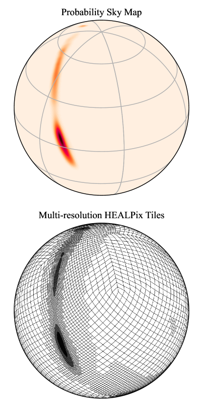
Figure 1: An example of the multi-resolution HEALPix sampling scheme that is used in GW localizations. The top panel shows the localization of LIGO/Virgo event GW200115_042309 (Abbott et al. 2021; GraceDB ID S200115j) as a heat map image; darker, deeper colors represent higher probability density. The bottom panel shows the boundaries of the multi-resolution HEALPix tiles on which the sky map was sampled.

The serialization format for GW sky maps is based upon multi-order coverage maps (MOCs; Fernique et al. 2014, 2019), an International Virtual Observatory Alliance (IVOA) specification for encoding footprints of observations or surveys as multi-resolution HEALPix bit masks to enable fast spatial unions and intersections. multi-order coverage maps are used extensively in the Aladin sky atlas (Bonnarel et al., 2000; Boch & Fernique, 2014) and many other Virtual Observatory (VO) tools and platforms. Greco et al. (2019) brought MOCs to prominence in the GW community by adding MOC contouring of GW probability maps and cross-matching with catalogs to Aladin. The hierarchical nature of HEALPix also underlies the IVOA hierarchical progressive surveys (HiPS) standard (Fernique et al., 2015, 2017), an astronomy map tile technology that enables interactive panning and zooming, similar to Google Maps, in Aladin.

1.2 HEALPix and Spatial Indices in Databases

There are a multitude of software packages that add HEALPix or similar spatial indices to common relational databases, including H3C (Landais et al., 2013), pg_healpix (Koposov, 2020), Q3C (Koposov & Bartunov, 2006, 2019), Hierarchical Triangular Mesh (HTM; Szalay et al. 2007), and pgSphere (Chilingarian et al., 2004). There is significant technological overlap with geospatial packages like PostGIS (Obe & Hsu, 2021). However, with the exception of PostGIS, these extensions and technologies do not naturally handle the image queries and arithmetic needed for directly processing multimessenger localizations.

Furthermore, all of these software packages are binary database extensions that must be specially installed or enabled on the server, making them difficult to deploy on robust, fault-tolerant, fully managed database services in the cloud, like Amazon Relational Database Service (RDS) (https://aws.amazon.com/rds/), Google Cloud SQL (https://cloud.google.com/sql), and Microsoft Azure Database for PostgreSQL (https://azure.microsoft.com/services/postgresql/). Out of all of the extensions listed above, only PostGIS is supported by these managed database services.

1.3 HEALPix in Python

There are many high-quality Python implementations of HEALPix. We list a few relevant ones here.

Healpy (Zonca et al., 2019) wraps the official HEALPix (Górski et al., 2005) C++ library as a NumPy (Harris et al., 2020) C extension. It is available as a stand-alone Python package from the Python Package Index, but is also included in the official polyglot HEALPix bundle. Healpy is the tool of choice for CMB analysis in Python because it exposes the underlying C++ library’s capability to transform HEALPix data sets to and from the space of spherical harmonics.

The astropy-healpix (Robitaille et al., 2020) project is a BSD-licensed Astropy-coordinated package with a high-level object-oriented interface and excellent integration with Astropy coordinates and units (Astropy Collaboration et al., 2013, 2018). Notably, astropy-healpix is used by the Astropy-coordinated reproject package to provide high-quality image reprojection between HEALPix and World Coordinate Systems (WCSs; Calabretta & Greisen 2002; Greisen & Calabretta 2002). Behind the scenes, astropy-healpix wraps a C implementation of HEALPix adapted from Astrometry.net (Lang et al., 2010).

MOCPy (Boch, 2019), developed at the Centre de Données astronomiques de Strasbourg (CDS), is an Astropy-affiliated package that provides fast manipulation of MOCs in Python, also with a high-level object-oriented interface. Its HEALPix support comes from the cdshealpix Python package, which wraps CDS’s implementation of HEALPix in the Rust programming language.

The most recent addition is mhealpy (Martinez-Castellanos et al., 2021), which combines some of the best features of Healpy, astropy-healpix, and MOCPy. The mhealpy package provides a unified object-oriented interface for conventional fixed-resolution HEALPix data sets (like Healpy and astropy-healpix) and multi-resolution data sets (like MOCPy). For MOCs, mhealpy supports not only region operations but also multi-resolution image arithmetic with a variety of options for normalization, making it a great choice for handling multi-resolution GW and GRB probability sky maps.

1.4 HEALPix Alchemy

One of several equivalent concrete data structures that can be used to encode multi-resolution HEALPix geometry is an interval set or range set (Reinecke & Hivon, 2015) consisting of a set of disjoint ranges of integer pixel indices. In the range set representation, calculating the union or intersection of any number of spatial regions reduces to simply merging sorted lists of integers. The range set data structure cuts across many areas of data science, from GWs (the authors acknowledge Kipp Cannon’s influential and elegant ligo-segments package, which has been one of the unsung heroes behind LIGO and Virgo observational results for years; see Cannon 2021) to bioinformatics (Alekseyenko & Lee, 2007; Stovner & Sætrom, 2019), not to mention obvious applications in business software. Because of the multitude of applications (frankly, in fields that are better funded than astronomy), there is a wealth of software for fast, general-purpose processing of range sets. PostgreSQL 14 was recently released with a new built-in multirange column type that maps perfectly onto the concept of HEALPix range sets.

In this paper, we introduce HEALPix Alchemy, a pure Python package that extends the popular SQLAlchemy database toolkit for Python (Bayer, 2012) to add fast multi-resolution HEALPix geometry on top of a PostgreSQL database using PostgreSQL 14 multiranges. HEALPix Alchemy accelerates queries involving cross-matches of points, regions, and images. Unlike traditional spatial indexing strategies, HEALPix Alchemy works with an unmodified PostgreSQL database service without any server-side extensions. HEALPix Alchemy can evaluate bulk queries involving unions of large numbers of regions ($\gtrsim$10) orders of magnitude faster than conventional, non-database multi-order HEALPix implementations like MOCPy. HEALPix Alchemy facilitates fast queries of GW sky maps by directly exploiting their native multi-resolution sampling.

The organization of the paper is as follows. In Section 2, we review the fundamentals and algebraic properties of HEALPix. In Section 3, we summarize the new multirange support in PostgreSQL. In Section 4, we explain the design, interface, and usage of HEALPix Alchemy. In Section 5, our sample code illustrates how to perform a variety of spatial queries that are important to a multimessenger broker or marshal application. Finally, in Section 6, our benchmarks show that the HEALPix Alchemy approach is fast and scalable. The code is open source and publicly available on GitHub (https://github.com/skyportal/healpix-alchemy) and Zenodo (Singer et al., 2021).

2 HEALPix Fundamentals

We begin by summarizing Górski et al. (2005) to provide a brief overview of HEALPix. HEALPix is both an all-sky map projection and a spatial indexing method. HEALPix divides and covers the unit sphere with equal-area tiles.

HEALPix may be thought of as a tree in which each node except for the root node has four children (see Fig. 2). At the lowest level in the tree, $l=0$, there are 12 base tiles, assigned integer indices $i=0,1,\dots,11$. At level $l=1$, each of the 12 base tiles is subdivided into 4 new tiles. Every subsequent level divides each of the preceding level’s tiles into 4 new tiles. At a given level $l$, each of the base tiles has been divided into $4^{l}$ tiles, i.e., $n_{\mathrm{side}}=2^{l}$ pixels on each side. Thus there are $n_{\mathrm{pix}}=12(4^{l})=12(n_{\mathrm{side}})^{2}$ pixels at a given resolution, assigned integer indices from $i=0,1,\dots,n_{\mathrm{pix}}-1$.

The angular size of HEALPix pixels varies from 59°at $l=0$, all the way down to 0.39 mas at $l=29$, the highest level at which the pixel index can be stored as a 64 bit signed integer without overflow.

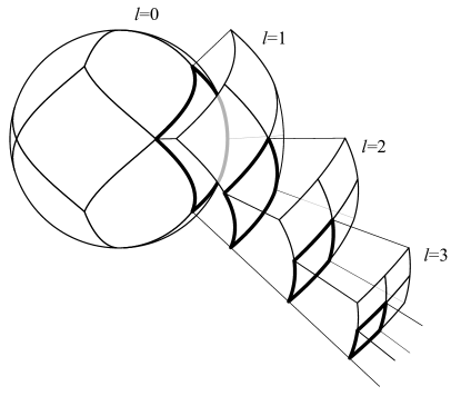
Figure 2: Illustration of the nested nature of HEALPix. Level 0 divides the unit sphere into 12 equal-area tiles. In each subsequent level, every tile is divided equally into four new tiles.

2.1 RING and NESTED Ordering

There are two conventional HEALPix pixel-ordering schemes, called RING and NESTED (see Fig. 3). At level $l=0$, the two ordering schemes are identical, but they differ at all higher orders. In the RING scheme, the pixel index $i$ advances first with R.A. from west to east and then with decl. from north to south. In the NESTED scheme, pixels that are siblings of one another in the HEALPix tree have consecutive values of pixel index.

Thus a HEALPix tile at any resolution is fully specified by a tuple of three values: the indexing scheme (RING or NESTED), the resolution level $l$ (or equivalently, $n_{\mathrm{side}}$), and the pixel index $i$. HEALPix software libraries typically provide two functions, one to convert from pixel index to R.A. and decl., and one to do the reverse. In Healpy (Zonca et al., 2019) these are called pix2ang and ang2pix respectively. In astropy-healpix (Robitaille et al., 2020), these are called healpix_to_lonlat and lonlat_to_healpix.

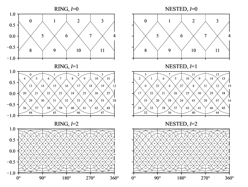
Figure 3: The first three levels of the HEALPix RING and NESTED indexing schemes. In each panel, the horizontal axis is R.A., and the vertical axis is the sine of the decl. After Górski et al. (2005).

The NESTED scheme has the delightful property that the base 4 digits of the pixel index $i$ encode the path all the way from the root of the HEALPix tree to the leaf tile. We may write a pixel index at any level $l^{*}$ in the mixed-radix form

$$i=\underbrace{(i_{0})_{12}}_{l=0}\underbrace{(i_{1})_{4}}_{l=1}\underbrace{(i_{2})_{4}}_{l=2}\dots\underbrace{(i_{l^{*}})_{4}}_{l=l^{*}},$$

which expands to

$$i=4^{(l^{*})}i_{0}+4^{(l^{*}-1)}i_{1}+4^{(l^{*}-2)}i_{2}+\dots+i_{l^{*}}.$$

There is yet a third pixel encoding called UNIQ (Reinecke & Hivon, 2015), which packs the resolution and the NESTED pixel index into a single integer:

$$u=i+4^{l+1}=i+4(n_{\mathrm{side}})^{2}.$$

The pixel index and resolution can be recovered from the UNIQ representation using bitwise operations.

2.2 HEALPix Image and Region Formats

Conventionally, the in-memory or on-disk (e.g., FITS file format; Pence et al. 2010) representation of an all-sky HEALPix image is a 1D array of length $n_{\mathrm{pix}}$. The $i$th value of the array is simply the value of the image sampled at the center of the pixel (or perhaps the value of the image integrated over the area of the pixel, depending on the application) with pixel index $i$. The ordering (RING or NESTED) and the uniform HEALPix resolution $n_{\mathrm{nside}}$ are stored as metadata. This flat-resolution format is prevalent in CMB applications and dust maps, and up through ’s and ’s second observing run (O2) was used as the native format for GW probability maps.

It is also possible to store a region on the sphere—for example, the footprint of an observation or of a survey—as a set of HEALPix pixels. Fig. 4 shows the footprint of the 47 deg² Zwicky Transient Facility (ZTF) camera as a MOC, consisting of a list of HEALPix tiles of mixed resolutions that are inside the region. The on-disk representation of a MOC in the Flexible Image Transport System (FITS) format is simply a 1D array of UNIQ indices. A MOC is typically a much more compact representation than a flat, fixed-resolution pixel mask: much of the interior of the region can be encoded using a small number of low-resolution tiles, and high-resolution tiles are only needed near the region’s boundary.

Figure 4: The 47 deg² footprint of the ZTF camera as a HEALPix MOC, refined to a maximum level of $l=10$. The left panel shows the footprint as a collection of filled polygons: each of the small filled squares is one CCD quadrant, each $2\times 2$ cluster of quadrants comprise a CCD, and the $4\times 4$ grid of CCDs comprise the entire focal plane. The middle panel shows the outlines of the multi-resolution HEALPix tiles that comprise the MOC. The inset panel at right shows a small portion of the MOC, with each pixel labeled with its resolution level $l$ and its nested pixel index $i$.

From ’s and ’s third observing run (O3) onward, the native format of GW probability sky maps is a multi-resolution FITS format based on the MOC format: it is table with one column containing the UNIQ pixel indices of each HEALPix tile, and additional columns containing floating-point values associated with each tile (see Fig. 1). Because GW sky maps are generated using an adaptive HEALPix mesh refinement scheme, devoting higher resolution to regions of higher probability density (Singer & Price, 2016), the savings in memory is substantial.

2.3 Range Sets

A final representation of a set of multi-resolution HEALPix tiles is as a range set. This is often the most computationally convenient form, and is the most important for this paper. One first selects a fixed maximum resolution level, typically $l_{\mathrm{max}}=29$ because it is the highest level at which pixel indices can fit in signed 64 bit integers. (Although unsigned 64 bit integers can hold $l_{\mathrm{max}}=30$ pixel indices, they are seldom used because most HEALPix libraries use the pixel index -1 to represent error conditions.) Now observe that a given HEALPix tile of level $l$ and pixel index $i$ contains all of the descendant pixels at level $l_{\mathrm{max}}$, such that their indices $i_{\mathrm{max}}$ are in the right-half-open interval,

$$\left[4^{(l_{\mathrm{max}}-l)}i,\,4^{(l_{\mathrm{max}}-l)}(i+1)\right).$$

Each tile in a MOC may be described by such an interval, and the MOC as a whole can be described by the integer set consisting of a union of disjoint intervals. That collection is called an interval set or a range set. Table 1 lists the pixels that are visible within the inset panel of Fig 4 as a range set.

HEALPix range sets are advantageous because the complicated problem of combining (e.g., taking the union or intersection of) multiple regions and merging overlapping tiles simplifies to the easier problem of combining sets of integer ranges. There is a straightforward algorithm to merge any number of range sets. In pseudocode:

1. Concatenate all of the range sets into a single list of ranges.

2. Sort the list of ranges by their lower bounds, breaking ties by their upper bounds.

3. Walk through the list element-by-element and merge overlapping endpoints.

Some MOC implementations like MOCPy provide only a binary union operator to merge a pair of range sets; if there are $k$ range sets and a total of $n$ ranges, then applying the above algorithm pairwise and recursively costs $O(nk\log n)$ time. However, the algorithm as written above supports an arbitrary number of ranges sets; it is dominated by the sort in Step 2 and costs only $O(n\log n)$ time. If there are $k$ range sets and they are presorted, then Steps 1 and 2 can be replaced by a $k$-way merge, and the algorithm completes in $O(n\log k)$ time (Mehlhorn & Sanders, 2008). If all of the intervals in all of the range sets are stored in a single presorted list to begin with (if, for example, they are stored in a single table in a relational database, with different range sets distinguished by a foreign key), then the element-by-element traversal in Step 3 dominates, and the algorithm completes in only $O(n)$ time.

This is a crucial point: we can evaluate unions of large numbers of regions ($k\gtrsim 10$) orders of magnitude faster if we store all of the ranges of all of the range sets in a single sorted data structure, in one table of a PostgreSQL database. The speedup is remarkable in the following example. There are $k=1830$ standard ZTF fields. The ZTF footprint with quadrant-level detail in Fig. 4 contains 826 HEALPix tiles down to $l=10$, for a total of $n\approx 1830\times 826=1{,}511{,}580$ HEALPix tiles. In this example, the database approach requires $k\log_{2}n\approx 4\times 10^{4}$ times fewer comparisons than the naive pairwise union approach, $\log_{2}n\approx 20$ times fewer comparisons than a naive $k$-way union approach, and $\log_{2}n/\log_{2}k\approx 2$ times fewer comparisons than an algorithm that does a $k$-way sorted merge.

There is also an efficient algorithm to test if a point is within a MOC, provided the range set is presorted. Calculate the level $l_{\mathrm{max}}$ pixel index of the point, then simply perform a bisection search to find a matching interval (or no matching interval) in $O(\log n)$ time.

Table 1: Range Set Example for the Inset from Fig. 4

$l$	$i$	UNIQ	Range Set (at $l=l_{\mathrm{max}}=29$)
⋮	⋮	⋮	⋮
8	300883	563027	[1323297428400504832, 1323301826447015936)
8	300892	563036	[1323337010819104768, 1323341408865615872)
⋮	⋮	⋮	⋮
9	1203525	2252101	[1323289731819110400, 1323290831330738176)
9	1203526	2252102	[1323290831330738176, 1323291930842365952)
9	1203527	2252103	[1323291930842365952, 1323293030353993728)
9	1203529	2252105	[1323294129865621504, 1323295229377249280)
9	1203557	2252133	[1323324916191199232, 1323326015702827008)
⋮	⋮	⋮	⋮
10	4808638	9002942	[1321788348691382272, 1321788623569289216)
⋮	⋮	⋮	⋮
10	4814093	9008397	[1323287807673761792, 1323288082551668736)
10	4814094	9008398	[1323288082551668736, 1323288357429575680)
10	4814095	9008399	[1323288357429575680, 1323288632307482624)
10	4814097	9008401	[1323288907185389568, 1323289182063296512)
10	4814098	9008402	[1323289182063296512, 1323289456941203456)
10	4814099	9008403	[1323289456941203456, 1323289731819110400)
10	4814113	9008417	[1323293305231900672, 1323293580109807616)
10	4814115	9008419	[1323293854987714560, 1323294129865621504)
10	4814124	9008428	[1323296328888877056, 1323296603766784000)
10	4814125	9008429	[1323296603766784000, 1323296878644690944)
10	4814127	9008431	[1323297153522597888, 1323297428400504832)
10	4814224	9008528	[1323323816679571456, 1323324091557478400)
10	4814225	9008529	[1323324091557478400, 1323324366435385344)
10	4814227	9008531	[1323324641313292288, 1323324916191199232)
10	4814236	9008540	[1323327115214454784, 1323327390092361728)
10	4814237	9008541	[1323327390092361728, 1323327664970268672)
10	4814239	9008543	[1323327939848175616, 1323328214726082560)
10	4814304	9008608	[1323345806912126976, 1323346081790033920)
⋮	⋮	⋮	⋮

3 PostgreSQL and Multiranges

PostgreSQL (Stonebraker & Rowe, 1986) is an established, popular, open-source, relational database management system with a Structured Query Language (SQL) interface. It is repackaged and sold by a variety of cloud providers as part of their flagship managed database services in Amazon RDS, Google Cloud SQL, Azure Database, and so on. It is a common choice of database for back ends of web applications, especially science applications and particularly astronomy brokers, target observation managers, and marshals.

One of many reasons for PostgreSQL’s popularity in the sciences is its wide variety of built-in data types. It may come as no surprise that PostgreSQL has supported range types since version 9.2.0, released in 2012. Specifically, the INT8RANGE type is ideal for storing ranges of 64 bit, 8 byte, $l_{\mathrm{max}}=29$ HEALPix indices, as described in the previous section. PostgreSQL defines many Boolean comparison operations on ranges: it can test if one range contains another, if one range overlaps another, if a range contains a scalar, etc. These operations are accelerated on columns that are indexed using the Generalized Search Tree (GiST; Hellerstein et al. 1995) or space-partitioned GiST (SP-GiST; Aref & Ilyas 2001) methods.

PostgreSQL 14.0, released on 2021 September 30, added two features that together make it possible to perform HEALPix MOC queries directly within the database. The first feature is a new multirange type, consisting of an array of ranges. The INT8MULTIRANGE type corresponds to HEALPix range sets described in the previous section. The second feature is the range_agg aggregate function, which takes ranges as its input and returns their union as a multirange.

4 HEALPix Alchemy

In all but the simplest web applications, it is common to generate database queries using a high-level abstraction layer rather than issuing hard-coded query statements directly. One of the more popular database abstraction libraries for Python is SQLAlchemy (Bayer, 2012), which allows one to express queries using Python syntax and provides a degree of independence between the code and the choice of database engine.

We have written HEALPix Alchemy, a Python package that extends SQLAlchemy to make it easy to work with multi-resolution HEALPix geometry. The match between HEALPix range sets and PostgreSQL multiranges is so perfect that HEALPix Alchemy consists of barely 100 lines of code (as measured using cloc; Danial 2021). We summarize the design of HEALPix Alchemy below.

4.1 Column Types

HEALPix Alchemy adds two custom SQLAlchemy column types (type decorators) that wrap the database’s own built-in SQL types: healpix_alchemy.Point and healpix_alchemy.Tile. For both column types, if a column is declared with the index=True keyword argument, HEALPix Alchemy automatically selects the space-partitioned GiST (SP-GiST) indexing method for that column.

4.1.1 The healpix_alchemy.Point Class

This class represents an infinitesimal point with no area, stored as a HEALPix NESTED pixel index at $l=l_{\mathrm{max}}=29$. A table containing a column of this type could hold a catalog of distant galaxies or a list of optical transients. It maps to the built-in PostgreSQL BIGINT type, a signed 64 bit integer. Values for healpix_alchemy.Point columns can be initialized from any of the following Python objects:

• an instance of astropy.coordinates.SkyCoord;

• a sequence of two astropy.units.Quantity instances with angle units, which will be interpreted as the R.A. and decl. of the point; or

• an integer representing the HEALPix NESTED index of the point at $l=l_{\mathrm{max}}=29$.

4.1.2 The healpix_alchemy.Tile Class

This class represents a multi-resolution HEALPix tile with finite area stored as a right-half-open interval of HEALPix NESTED pixel indices at $l=l_{\mathrm{max}}=29$. It maps to the built-in PostgreSQL INT8RANGE type, which is the range type corresponding to BIGINT. A table containing a column of this type could store MOCs or GW probability maps. Values for healpix_alchemy.Tile columns can be initialized from any of the following Python objects:

• a single integer that will be interpreted as the address of the tile in the UNIQ indexing scheme;

• a sequence of two integers like (1234, 5678), which will be interpreted as the lower and upper bounds of the right-half-open pixel index interval at $l=l_{\mathrm{max}}=29$; or

• a string like '[1234,5678)', which is the canonical string representation of an INT8RANGE in PostgreSQL.

There is also a factory method healpix_alchemy.Tile.tiles_from that returns a collection of Python values suitable for initializing multiple healpix_alchemy.Tile values. It accepts either of the following Python objects:

• an instance of astropy.coordinates.SkyCoord containing a vector of coordinates representing the vertices of a spherical polygon, which is converted to a MOC with a default refinement level of $l=10$ using MOCPy (Boch, 2019); or

• an instance of mocpy.MOC.

The healpix_alchemy.Tile class provides the following properties:

• healpix_alchemy.Tile.lower, returning the left (closed) bound of the interval;

• healpix_alchemy.Tile.upper, returning the right (open) bound of the interval;

• healpix_alchemy.Tile.length, returning the difference of the right and left bounds; and

• healpix_alchemy.Tile.area, returning the area of the tile in steradians.

Note that we do not provide a type decorator for the INT8MULTIRANGE type itself because in most applications it should be more efficient to store ranges rather than multiranges in tables.

4.2 Aggregate Functions

HEALPix Alchemy provides the function healpix_alchemy.func.union to find the union of HEALPix ranges. Because it involves a SQL aggregate function, generally it should be used in a subquery (examples to follow). The Python expression healpix_alchemy.func.union(x) maps to the SQL expression unnest(range_agg(x)).

5 Sample Code

In this section, we provide some Python sample code using HEALPix Alchemy to perform the most common queries that one needs in a multimessenger astronomy broker or marshal.

5.1 Installation

HEALPix Alchemy requires Python 3.7 or later. To install HEALPix Alchemy and all of its Python dependencies from the Python Package Index using the pip package manager, simply run the following command in a terminal:

⬇

pip install healpix-alchemy

5.2 Imports and Setup

We begin with some imports:

⬇

import sqlalchemy as sa

from sqlalchemy.ext.declarative import (

as_declarative, declared_attr)

import healpix_alchemy as ha

SQLAlchemy needs to know the name for each table. You could provide the name by setting the __tablename__ attribute in each Python model class, but it is common practice to create a base class that generates the table name automatically from the Python class name:

⬇

@as_declarative()

class Base:

@declared_attr

def __tablename__(cls):

return cls.__name__.lower()

5.3 Model Classes

Next, we declare Python classes that will correspond to tables in the database. Each row of the Galaxy table represents a point in a galaxy catalog:

⬇

class Galaxy(Base):

id = sa.Column(

sa.Text, primary_key=True)

hpx = sa.Column(

ha.Point, index=True, nullable=False)

Each row of the Field table represents the footprint of a ZTF standard field:

⬇

class Field(Base):

id = sa.Column(

sa.Integer, primary_key=True)

tiles = sa.orm.relationship(

lambda: FieldTile)

Each row of the FieldTile table represents a multi-resolution HEALPix tile that is contained within the corresponding field. There is a one-to-many mapping between Field and FieldTile.

⬇

class FieldTile(Base):

id = sa.Column(

sa.ForeignKey(Field.id), primary_key=True)

hpx = sa.Column(

ha.Tile, primary_key=True, index=True)

Each row of the Skymap table represents a GW HEALPix localization map:

⬇

class Skymap(Base):

id = sa.Column(

sa.Integer, primary_key=True)

tiles = sa.orm.relationship(

lambda: SkymapTile)

Each row of the SkymapTile table represents a multi-resolution HEALPix tile with an associated probability density within a GW localization map. There is a one-to-many mapping between Skymap and SkymapTile.

⬇

class SkymapTile(Base):

id = sa.Column(

sa.ForeignKey(Skymap.id),

primary_key=True)

hpx = sa.Column(

ha.Tile, primary_key=True, index=True)

probdensity = sa.Column(

sa.Float, nullable=False)

Finally, connect to the database, create all the tables, and start a session (replacing user, password, host, and database with the username, password, hostname, and database name respectively that you use to connect to your PostgreSQL database:

⬇

url = 'postgresql://user:password@host/database'

engine = sa.create_engine(url)

Base.metadata.create_all(engine)

session = sa.orm.Session(engine)

5.4 Populate with Sample Data

Now we populate the tables with some sample data. First, we load the Two Micron All Sky Survey (2MASS) Redshift Survey (Huchra et al., 2012) into the Galaxy table. This catalog contains 44,599 galaxies. (It may take up to a minute for this to finish. Advanced users may speed this up significantly by vectorizing the conversion from SkyCoord to HEALPix indices and using SQLAlchemy bulk insertion.)

⬇

from astropy.coordinates import SkyCoord

from astroquery.vizier import Vizier

catalog_name = 'J/ApJS/199/26/table3'

columns = ['SimbadName', 'RAJ2000', 'DEJ2000']

vizier = Vizier(columns=columns, row_limit=-1)

cat, = vizier.get_catalogs(catalog_name)

coords = SkyCoord(cat['RAJ2000'], cat['DEJ2000'])

for name, coord in zip(cat['SimbadName'], coords):

session.add(Galaxy(id=name, hpx=coord))

session.commit()

Next, we load the footprints of the ZTF standard fields into the Field and FieldTile tables. (It may take up to a minute for this to finish too. Advanced users may speed this up significantly by using SQLAlchemy bulk insertion.)

⬇

from astropy.table import Table

from astropy.coordinates import SkyCoord

from astropy import units as u

url = 'https://raw.githubusercontent.com/ZwickyTransientFacility/ztf_information/master/field_grid/ztf_field_corners.csv'

for row in Table.read(url):

id = int(row['field'])

ras = row['ra1', 'ra2', 'ra3', 'ra4']

decs = row['dec1', 'dec2', 'dec3', 'dec4']

corners = SkyCoord(ras, decs, unit=u.deg)

tiles = [

FieldTile(hpx=hpx)

for hpx in ha.Tile.tiles_from(corners)]

session.add(Field(id=id, tiles=tiles))

session.commit()

Lastly, we load a sky map for LIGO/Virgo event GW200115_042309 (Abbott et al. 2021; GraceDB ID S200115j) into the Skymap and SkymapTile tables.

⬇

url = 'https://gracedb.ligo.org/apiweb/superevents/S200115j/files/bayestar.multiorder.fits'

data = Table.read(url)

tiles = [

SkymapTile(

hpx=row['UNIQ'],

probdensity=row['PROBDENSITY'])

for row in data]

session.add(Skymap(id=1, tiles=tiles))

session.commit()

5.5 Example Queries

Now we provide some examples of common queries that would occur in a multimessenger astronomy broker or marshal. (In all of the examples below, we limit the result set to 5 rows to avoid generating a large amount of terminal output.)

5.5.1 What Is the Area of Each Field?

The area of a region is simply the sum of the area of all of the HEALPix tiles that belong to the region. The following query:

⬇

query = session.query(

FieldTile.id, sa.func.sum(FieldTile.hpx.area)

).group_by(

FieldTile.id

).limit(

5

)

for id, area in session.execute(query):

print(f'Field {id} has area {area:.3g} sr')

produces this output:

⬇

Field 199 has area 0.0174 sr

Field 200 has area 0.0174 sr

Field 201 has area 0.0174 sr

Field 202 has area 0.0174 sr

Field 203 has area 0.0174 sr

5.5.2 How Many Galaxies Are in Each Field?

For this query, we need to introduce the contains comparison function, which tests if a healpix_alchemy.Tile contains a healpix_alchemy.Point. Behind the scenes, this simply maps to the built-in PostgreSQL @> comparison operator. The following query:

⬇

count = sa.func.count(Galaxy.id)

query = session.query(

FieldTile.id, count

).filter(

FieldTile.hpx.contains(Galaxy.hpx)

).group_by(

FieldTile.id

).order_by(

count.desc()

).limit(

5

)

for id, n in session.execute(query):

print(f'Field {id} contains {n} galaxies')

produces this output:

⬇

Field 1739 contains 343 galaxies

Field 699 contains 336 galaxies

Field 700 contains 311 galaxies

Field 225 contains 303 galaxies

Field 1740 contains 289 galaxies

5.5.3 What Is the Probability Density at the Position of Each Galaxy?

Since sky map tiles and region tiles are represented using the same healpix_alchemy.Tile column type; this is just a minor variation on the previous query. The following:

⬇

query = session.query(

Galaxy.id, SkymapTile.probdensity

).filter(

SkymapTile.id == 1,

SkymapTile.hpx.contains(Galaxy.hpx)

).order_by(

SkymapTile.probdensity.desc()

).limit(

5

)

for id, p in session.execute(query):

print(f'{id} has prob. density {p:.5g}/sr')

produces this output:

⬇

2MASX J02532153+0632222 has prob. density 20.701/sr

2MASX J02530482+0555431 has prob. density 20.695/sr

2MASX J02533119+0628252 has prob. density 20.669/sr

2MASX J02524584+0639206 has prob. density 20.656/sr

2MASX J02534120+0615562 has prob. density 20.567/sr

5.5.4 What Is the Probability Contained within Each Field?

For this query, we need to introduce the overlaps comparison function, which tests if one healpix_alchemy.Tile overlaps another. Behind the scenes, this simply maps to the built-in PostgreSQL && comparison operator. We also need the * operator, which returns a new tile that is the intersection of two tiles. The following query:

⬇

area = (FieldTile.hpx * SkymapTile.hpx).area

prob = sa.func.sum(SkymapTile.probdensity * area)

query = session.query(

FieldTile.id, prob

).filter(

SkymapTile.id == 1,

FieldTile.hpx.overlaps(SkymapTile.hpx)

).group_by(

FieldTile.id

).order_by(

prob.desc()

).limit(

5

)

for id, prob in session.execute(query):

print(f'Field {id} probability is {prob:.3g}')

produces this output:

⬇

Field 1499 probability is 0.165

Field 1446 probability is 0.156

Field 452 probability is 0.154

Field 505 probability is 0.0991

Field 401 probability is 0.0962

5.5.5 What Is the Combined Area of Fields 1000 through 2000?

In the next two examples, we introduce healpix_alchemy.func.union(), which finds the union of a set of tiles. Because it is an aggregate function, it should generally be used in a subquery. The following:

⬇

union = session.query(

ha.func.union(FieldTile.hpx).label('hpx')

).filter(

FieldTile.id.between(1000, 2000)

).subquery()

query = session.query(

sa.func.sum(union.columns.hpx.area)

)

result = session.execute(query).scalar_one()

print(f'{result:.3g} sr')

produces this output:

⬇

9.33 sr

5.5.6 What Is the Integrated Probability Contained within Fields 1000 through 2000?

This is a minor variation on the previous query. The following:

⬇

union = session.query(

ha.func.union(FieldTile.hpx).label('hpx')

).filter(

FieldTile.id.between(1000, 2000)

).subquery()

area = (union.columns.hpx * SkymapTile.hpx).area

prob = sa.func.sum(SkymapTile.probdensity * area)

query = session.query(

prob

).filter(

SkymapTile.id == 1,

union.columns.hpx.overlaps(SkymapTile.hpx)

)

result = session.execute(query).scalar_one()

print(f'{result:.3g}')

produces this output:

⬇

0.837

5.5.7 What Is the Area of the 90% Credible Region?

The 90% credible region of a GW probability sky map is defined as the region with the smallest area that has a 90% probability of containing the true location of the GW source. To find the HEALPix tiles that are within the 90% credible region, we have to rank the tiles by descending probability density, then calculate the cumulative sum of their probability (probability density times area), and then search for the tile that has a cumulative probability of 0.9.

In SQL, a cumulative is expressed as a window expression, using an over clause. This query involves such a clause as well as a subquery. The following:

⬇

# Assemble the expression representing the

# cumulative area of credible levels

cum_area = sa.func.sum(

SkymapTile.hpx.area

).over(

order_by=SkymapTile.probdensity.desc()

).label(

'cum_area'

)

# Assemble the expression representing the

# cumulative probability of credible levels

cum_prob = sa.func.sum(

SkymapTile.probdensity * SkymapTile.hpx.area

).over(

order_by=SkymapTile.probdensity.desc()

).label(

'cum_prob'

)

# Query cumulative area and probability of

# credible levels

subquery = session.query(

cum_area, cum_prob

).filter(

SkymapTile.id == 1

).subquery()

# Find cumulative area at which

# cumulative probability reaches 90%

query = session.query(

sa.func.max(subquery.columns.cum_area)

).filter(

subquery.columns.cum_prob <= 0.9

)

result = session.execute(query).scalar_one()

print(f'{result:.3g} sr')

produces this output:

⬇

0.277 sr

5.5.8 Which Galaxies Are within the 90% Credible Region?

This is just a minor variation on the previous query. The following:

⬇

# Assemble the expression representing the

# cumulative probability of credible levels

cum_prob = sa.func.sum(

SkymapTile.probdensity * SkymapTile.hpx.area

).over(

order_by=SkymapTile.probdensity.desc()

).label(

'cum_prob'

)

# Query probability density

# and cumulative probability

subquery = session.query(

SkymapTile.probdensity, cum_prob

).filter(

SkymapTile.id == 1

).subquery()

# Find probability density at which

# cumulative probablity reaches 90%

min_probdensity = session.query(

sa.func.min(subquery.columns.probdensity)

).filter(

subquery.columns.cum_prob <= 0.9

).scalar_subquery()

# Query galaxies that have probability density

# great than or equal to that on boundary of

# the 90% credible level

query = session.query(

Galaxy.id

).filter(

SkymapTile.id == 1,

SkymapTile.hpx.contains(Galaxy.hpx),

SkymapTile.probdensity >= min_probdensity

).limit(

5

)

for galaxy_id, in session.execute(query):

print(galaxy_id)

produces this output:

⬇

2MASX J02424077-0000478

2MASX J02352772-0921216

2MASX J02273746-0109226

2MASX J02414523+0026354

2MASX J20095408-4822462

6 Performance

To measure the performance of HEALPix Alchemy, we populated a test database with a $N_{\mathrm{gal}}=40\mathrm{k}$ randomly and isotropically distributed galaxies, a randomly subdivided sky map with $N_{\mathrm{skymap}}=20\mathrm{k}$ HEALPix tiles, and $N_{\mathrm{field}}$=1–10k random and isotropically distributed square fields with the dimensions of the ZTF camera.

We measured the performance of a few representative queries based on those in the previous section:

1. Find area of union: Find the area in steradians of all $N_{\mathrm{field}}$ fields.

2. Cross-match with 40k galaxies: Count the number of galaxies within each of the $N_{\mathrm{field}}$ fields.

3. Find fields in 90% cred. region: Count how many of the $N_{\mathrm{field}}$ fields are within the 90% credible region of the sky map.

(Queries 2 and 3 count the number of matching galaxies or fields rather than listing in order to limit the amount of output sent back to the client while still causing PostgreSQL to enumerate all of the matching rows.)

To gather benchmarks on Amazon Web Services (AWS), we configured a PostgreSQL 14 database in the RDS Database Preview Environment on one db.m5.xlarge instance. We installed Ubuntu 20.04 LTS (“Focal Fossa”) and HEALPix Alchemy on an Elastic Compute Cloud (EC2) instance in the same availability zone as the database. Both the RDS and the EC2 instances ran on Intel Xeon Platinum 8000 series CPUs and had 4 virtual cores and 16 GiB of memory (Amazon, 2021).

For small numbers of fields, we find that HEALPix Alchemy queries are comparable in run time to equivalent Python code using MOCPy. However, as the number of fields grows into the hundreds or thousands, HEALPix Alchemy is orders of magnitude faster than MOCPy, because in the database the tiles belonging to all of the MOCs are indexed and presorted as a single table.

Fig. 5 plots the run time in seconds of all three queries as a function of the number of fields, $N_{\mathrm{field}}$. Within the domain of this plot, all three queries exhibit roughly linear scaling. There are $N_{\mathrm{field}}=1830$ standard ZTF fields. Reading off of the plot, for this database size all three queries complete within about a second—suitable for use in an interactive web application.

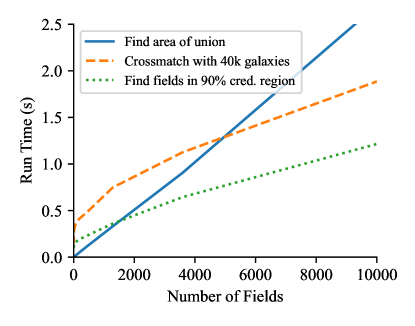
Figure 5: Run time on AWS as a function of the number of fields of three representative queries in HEALPix Alchemy.

7 Conclusion

The new multirange type in PostgreSQL 14 is perfect for storing HEALPix range sets, facilitating spatial region and image queries that are the bread and butter of a multimessenger astronomy broker or marshal. We have provided the minimalist HEALPix Alchemy package to make it easier to express these queries in Python.

HEALPix Alchemy is built on the solid foundations of several existing high-quality open-source HEALPix and MOC implementations in Python. Specifically, HEALPix Alchemy integrates with Astropy and MOCPy to populate PostgreSQL tables from a variety of Python types. However, once spatial data are within the database, HEALPix Alchemy queries significantly outperform MOCPy for bulk operations on large numbers of MOCs because PostgreSQL can store all of the HEALPix tiles for all of the regions or sky maps in a single, coherently indexed table.

Our technique works with a stock PostgreSQL 14 server without any patches or extensions—an important feature because web applications often demand the robustness of a fully managed cloud database service. At the time of this writing, PostgreSQL 14 is supported by all three major cloud providers: Amazon RDS (Amazon, 2022), Google Cloud SQL (Google, 2022), and (in some regions) Microsoft Azure Database (Erdogan, 2021).

HEALPix Alchemy provides spatial indexing for SkyPortal (van der Walt et al., 2019), a general-purpose astronomical data portal, of which the ZTF follow-up marshal, Fritz, is an instance. We are currently working on consolidating the multimessenger functionality of the GROWTH ToO Marshal (Anand et al., 2021) into SkyPortal using HEALPix Alchemy for greatly improved performance. We expect that the HEALPix Alchemy technique will be widely applicable to science portals in the multimessenger astronomy era, including NASA’s recently proposed Multimessenger Astrophysics Support Center (Sambruna et al., 2021).

References

- Aartsen et al. (2017) Aartsen, M. G., Ackermann, M., Adams, J., et al. 2017, Astroparticle Physics, 92, 30, doi: 10.1016/j.astropartphys.2017.05.002
- Abbott et al. (2018) Abbott, B. P., Abbott, R., Abbott, T. D., et al. 2018, Living Reviews in Relativity, 21, 3, doi: 10.1007/s41114-018-0012-9
- Abbott et al. (2021) Abbott, R., Abbott, T. D., Abraham, S., et al. 2021, ApJ, 915, L5, doi: 10.3847/2041-8213/ac082e
- Acernese et al. (2015) Acernese, F., Agathos, M., Agatsuma, K., et al. 2015, Classical and Quantum Gravity, 32, 024001, doi: 10.1088/0264-9381/32/2/024001
- Akutsu et al. (2021) Akutsu, T., Ando, M., Arai, K., et al. 2021, Progress of Theoretical and Experimental Physics, 2021, 05A101, doi: 10.1093/ptep/ptaa125
- Alekseyenko & Lee (2007) Alekseyenko, A. V., & Lee, C. J. 2007, Bioinformatics, 23, 1386, doi: 10.1093/bioinformatics/btl647
- Amazon (2021) Amazon. 2021, Amazon EC2 M5 Instances. https://aws.amazon.com/ec2/instance-types/m5/
- Amazon (2022) —. 2022, PostgreSQL on Amazon RDS. https://web.archive.org/web/20220318061718/https://docs.aws.amazon.com/AmazonRDS/latest/UserGuide/CHAP_PostgreSQL.html
- Anand et al. (2021) Anand, S., Andreoni, I., Goldstein, D. A., et al. 2021, in Revista Mexicana de Astronomia y Astrofisica Conference Series, Vol. 53, Revista Mexicana de Astronomia y Astrofisica Conference Series, 91–99, doi: 10.22201/ia.14052059p.2021.53.20
- Aref & Ilyas (2001) Aref, W., & Ilyas, I. 2001, J. Intell. Inf. Syst., 17, 215, doi: 10.1023/A:1012809914301
- Astropy Collaboration et al. (2013) Astropy Collaboration, Robitaille, T. P., Tollerud, E. J., et al. 2013, A&A, 558, A33, doi: 10.1051/0004-6361/201322068
- Astropy Collaboration et al. (2018) Astropy Collaboration, Price-Whelan, A. M., Sipőcz, B. M., et al. 2018, AJ, 156, 123, doi: 10.3847/1538-3881/aabc4f
- Bayer (2012) Bayer, M. 2012, in The Architecture of Open Source Applications Volume II: Structure, Scale, and a Few More Fearless Hacks, ed. A. Brown & G. Wilson (aosabook.org). http://aosabook.org/en/sqlalchemy.html
- Bellm et al. (2019) Bellm, E. C., Kulkarni, S. R., Graham, M. J., et al. 2019, PASP, 131, 018002, doi: 10.1088/1538-3873/aaecbe
- Boch (2019) Boch, T. 2019, in Astronomical Society of the Pacific Conference Series, Vol. 521, Astronomical Data Analysis Software and Systems XXVI, ed. M. Molinaro, K. Shortridge, & F. Pasian, 487
- Boch & Fernique (2014) Boch, T., & Fernique, P. 2014, in Astronomical Society of the Pacific Conference Series, Vol. 485, Astronomical Data Analysis Software and Systems XXIII, ed. N. Manset & P. Forshay, 277
- Bonnarel et al. (2000) Bonnarel, F., Fernique, P., Bienaymé, O., et al. 2000, A&AS, 143, 33, doi: 10.1051/aas:2000331
- Brown et al. (2013) Brown, T. M., Baliber, N., Bianco, F. B., et al. 2013, PASP, 125, 1031, doi: 10.1086/673168
- Calabretta & Greisen (2002) Calabretta, M. R., & Greisen, E. W. 2002, A&A, 395, 1077, doi: 10.1051/0004-6361:20021327
- Cannon (2021) Cannon, K. 2021, ligo-segments. https://git.ligo.org/lscsoft/ligo-segments
- Chilingarian et al. (2004) Chilingarian, I., Bartunov, O., Richter, J., & Sigaev, T. 2004, in Astronomical Society of the Pacific Conference Series, Vol. 314, Astronomical Data Analysis Software and Systems (ADASS) XIII, ed. F. Ochsenbein, M. G. Allen, & D. Egret, 225
- Connaughton et al. (2015) Connaughton, V., Briggs, M. S., Goldstein, A., et al. 2015, ApJS, 216, 32, doi: 10.1088/0067-0049/216/2/32
- Coughlin (2020) Coughlin, M. W. 2020, Nature Astronomy, 4, 550, doi: 10.1038/s41550-020-1130-3
- Danial (2021) Danial, A. 2021, cloc: v1.92, v1.92, Zenodo, doi: 10.5281/zenodo.5760077
- Dekany et al. (2020) Dekany, R., Smith, R. M., Riddle, R., et al. 2020, PASP, 132, 038001, doi: 10.1088/1538-3873/ab4ca2
- Erdogan (2021) Erdogan, O. 2021, How We Shipped PostgreSQL 14 on Azure Within One Day of its Release, Microsoft. https://techcommunity.microsoft.com/t5/azure-database-for-postgresql/how-we-shipped-postgresql-14-on-azure-within-one-day-of-its/ba-p/2801300
- Fernique et al. (2014) Fernique, P., Boch, T., Donaldson, T., et al. 2014, MOC - HEALPix Multi-Order Coverage map Version 1.0, IVOA Recommendation 02 June 2014, doi: 10.5479/ADS/bib/2014ivoa.spec.0602F
- Fernique et al. (2019) —. 2019, MOC - HEALPix Multi-Order Coverage map Version 1.1, IVOA Recommendation 07 October 2019
- Fernique et al. (2015) Fernique, P., Allen, M. G., Boch, T., et al. 2015, A&A, 578, A114, doi: 10.1051/0004-6361/201526075
- Fernique et al. (2017) Fernique, P., Allen, M., Boch, T., et al. 2017, HiPS - Hierarchical Progressive Survey Version 1.0, IVOA Recommendation 19 May 2017, doi: 10.5479/ADS/bib/2017ivoa.spec.0519F
- Förster et al. (2021) Förster, F., Cabrera-Vives, G., Castillo-Navarrete, E., et al. 2021, AJ, 161, 242, doi: 10.3847/1538-3881/abe9bc
- Ginsburg et al. (2019) Ginsburg, A., Sipőcz, B. M., Brasseur, C. E., et al. 2019, AJ, 157, 98, doi: 10.3847/1538-3881/aafc33
- Goldstein et al. (2020) Goldstein, A., Fletcher, C., Veres, P., et al. 2020, ApJ, 895, 40, doi: 10.3847/1538-4357/ab8bdb
- Google (2022) Google. 2022, Database versions and version policies. https://web.archive.org/web/20220119055010/https://cloud.google.com/sql/docs/postgres/db-versions
- Górski et al. (2005) Górski, K. M., Hivon, E., Banday, A. J., et al. 2005, ApJ, 622, 759, doi: 10.1086/427976
- Graham et al. (2019) Graham, M. J., Kulkarni, S. R., Bellm, E. C., et al. 2019, PASP, 131, 078001, doi: 10.1088/1538-3873/ab006c
- Greco et al. (2019) Greco, G., Branchesi, M., Chassande-Mottin, E., et al. 2019, in Proceedings of The New Era of Multi-Messenger Astrophysics — PoS(Asterics2019), Vol. 357, 031, doi: 10.22323/1.357.0031
- Greisen & Calabretta (2002) Greisen, E. W., & Calabretta, M. R. 2002, A&A, 395, 1061, doi: 10.1051/0004-6361:20021326
- Harris et al. (2020) Harris, C. R., Millman, K. J., van der Walt, S. J., et al. 2020, Nature, 585, 357, doi: 10.1038/s41586-020-2649-2
- Hellerstein et al. (1995) Hellerstein, J. M., Naughton, J. F., & Pfeffer, A. 1995, in Proceedings of the 21th International Conference on Very Large Data Bases, VLDB ’95 (San Francisco, CA, USA: Morgan Kaufmann Publishers Inc.), 562–573
- Huchra et al. (2012) Huchra, J. P., Macri, L. M., Masters, K. L., et al. 2012, ApJS, 199, 26, doi: 10.1088/0067-0049/199/2/26
- Hunter (2007) Hunter, J. D. 2007, Computing in Science and Engineering, 9, 90, doi: 10.1109/MCSE.2007.55
- Ivezić et al. (2019) Ivezić, Ž., Kahn, S. M., Tyson, J. A., et al. 2019, ApJ, 873, 111, doi: 10.3847/1538-4357/ab042c
- Kasliwal et al. (2019) Kasliwal, M. M., Cannella, C., Bagdasaryan, A., et al. 2019, PASP, 131, 038003, doi: 10.1088/1538-3873/aafbc2
- Kasliwal et al. (2020) Kasliwal, M. M., Anand, S., Ahumada, T., et al. 2020, ApJ, 905, 145, doi: 10.3847/1538-4357/abc335
- Koposov (2020) Koposov, S. 2020, pg_healpix. https://github.com/segasai/pg_healpix
- Koposov & Bartunov (2006) Koposov, S., & Bartunov, O. 2006, in Astronomical Society of the Pacific Conference Series, Vol. 351, Astronomical Data Analysis Software and Systems XV, ed. C. Gabriel, C. Arviset, D. Ponz, & S. Enrique, 735
- Koposov & Bartunov (2019) Koposov, S., & Bartunov, O. 2019, Q3C: A PostgreSQL package for spatial queries and cross-matches of large astronomical catalogs. http://ascl.net/1905.008
- Landais et al. (2013) Landais, G., Ochsenbein, F., & Simon, A. 2013, in Astronomical Society of the Pacific Conference Series, Vol. 475, Astronomical Data Analysis Software and Systems XXII, ed. D. N. Friedel, 227
- Lang et al. (2010) Lang, D., Hogg, D. W., Mierle, K., Blanton, M., & Roweis, S. 2010, AJ, 139, 1782, doi: 10.1088/0004-6256/139/5/1782
- Las Cumbres Observatory (2019) Las Cumbres Observatory. 2019, in TOM Toolkit Workshop. https://lco.global/workshops/tom-toolkit-community-workshop/
- LIGO Scientific Collaboration et al. (2015) LIGO Scientific Collaboration, Aasi, J., Abbott, B. P., et al. 2015, Classical and Quantum Gravity, 32, 074001, doi: 10.1088/0264-9381/32/7/074001
- Martinez-Castellanos et al. (2021) Martinez-Castellanos, I., Singer, L. P., Burns, E., et al. 2021, arXiv e-prints, arXiv:2111.11240. https://arxiv.org/abs/2111.11240
- Masci et al. (2019) Masci, F. J., Laher, R. R., Rusholme, B., et al. 2019, PASP, 131, 018003, doi: 10.1088/1538-3873/aae8ac
- Matheson et al. (2021) Matheson, T., Stubens, C., Wolf, N., et al. 2021, AJ, 161, 107, doi: 10.3847/1538-3881/abd703
- Meegan et al. (2009) Meegan, C., Lichti, G., Bhat, P. N., et al. 2009, ApJ, 702, 791, doi: 10.1088/0004-637X/702/1/791
- Mehlhorn & Sanders (2008) Mehlhorn, K., & Sanders, P. 2008, Algorithms and Data Structures: The Basic Toolbox, SpringerLink: Springer e-Books (Springer Berlin Heidelberg). https://books.google.com/books?id=H2BDafez-A0C
- Möller et al. (2021) Möller, A., Peloton, J., Ishida, E. E. O., et al. 2021, MNRAS, 501, 3272, doi: 10.1093/mnras/staa3602
- Nordin et al. (2019) Nordin, J., Brinnel, V., van Santen, J., et al. 2019, A&A, 631, A147, doi: 10.1051/0004-6361/201935634
- Obe & Hsu (2021) Obe, R., & Hsu, L. 2021, PostGIS in Action, Third Edition (Manning). https://books.google.com/books?id=6PY8EAAAQBAJ
- Pence et al. (2010) Pence, W. D., Chiappetti, L., Page, C. G., Shaw, R. A., & Stobie, E. 2010, A&A, 524, A42, doi: 10.1051/0004-6361/201015362
- Petrov et al. (2022) Petrov, P., Singer, L. P., Coughlin, M. W., et al. 2022, ApJ, 924, 54, doi: 10.3847/1538-4357/ac366d
- Raen (2021) Raen, T. 2021, Pitt-Google Alert Broker. https://github.com/mwvgroup/Pitt-Google-Broker
- Reinecke & Hivon (2015) Reinecke, M., & Hivon, E. 2015, A&A, 580, A132, doi: 10.1051/0004-6361/201526549
- Robitaille et al. (2020) Robitaille, T., Deil, C., & Ginsburg, A. 2020, reproject: Python-based astronomical image reprojection. http://ascl.net/2011.023
- Sambruna et al. (2021) Sambruna, R. M., Schlieder, J. E., Kocevski, D., et al. 2021, arXiv e-prints, arXiv:2109.10841. https://arxiv.org/abs/2109.10841
- Singer et al. (2021) Singer, L., Goldstein, D., Crellin-Quick, A., Parazin, B., & Coughlin, M. 2021, skyportal/healpix-alchemy: Version 1.0.1, v1.0.1, Zenodo, doi: 10.5281/zenodo.5768564
- Singer & Price (2016) Singer, L. P., & Price, L. R. 2016, Phys. Rev. D, 93, 024013, doi: 10.1103/PhysRevD.93.024013
- Singer et al. (2016) Singer, L. P., Chen, H.-Y., Holz, D. E., et al. 2016, ApJ, 829, L15, doi: 10.3847/2041-8205/829/1/L15
- Smith et al. (2019) Smith, K. W., Williams, R. D., Young, D. R., et al. 2019, Research Notes of the American Astronomical Society, 3, 26, doi: 10.3847/2515-5172/ab020f
- Stonebraker & Rowe (1986) Stonebraker, M., & Rowe, L. A. 1986, in Proceedings of the 1986 ACM SIGMOD International Conference on Management of Data, SIGMOD ’86 (New York, NY, USA: Association for Computing Machinery), 340–355, doi: 10.1145/16894.16888
- Stovner & Sætrom (2019) Stovner, E. B., & Sætrom, P. 2019, Bioinformatics, 36, 918, doi: 10.1093/bioinformatics/btz615
- Szalay et al. (2007) Szalay, A. S., Gray, J., Fekete, G., et al. 2007, arXiv e-prints, cs/0701164. https://arxiv.org/abs/cs/0701164
- van der Walt et al. (2019) van der Walt, S., Crellin-Quick, A., & Bloom, J. 2019, The Journal of Open Source Software, 4, 1247, doi: 10.21105/joss.01247
- Wyatt et al. (2020) Wyatt, S. D., Tohuvavohu, A., Arcavi, I., et al. 2020, ApJ, 894, 127, doi: 10.3847/1538-4357/ab855e
- Zonca et al. (2019) Zonca, A., Singer, L., Lenz, D., et al. 2019, The Journal of Open Source Software, 4, 1298, doi: 10.21105/joss.01298