Mixed leptonic and hadronic corrections to the
anomalous magnetic moment of the muon

Abstract

Higher-order hadronic corrections to the anomalous magnetic moment of the muon have been evaluated including next-to-next-to-leading-order insertions of hadronic vacuum polarization and next-to-leading-order corrections to hadronic light-by-light scattering. This leaves a set of mixed leptonic and hadronic corrections in the form of double-bubble topologies as the only remaining hadronic effect at $\mathcal{O}(\alpha^{4})$. Here, we estimate these contributions by analyzing the respective cuts of the diagrams, suggesting that the impact is limited to $\lesssim 1\times 10^{-11}$ and thus negligible at the level of the final precision of the Fermilab $g-2$ experiment.

Introduction.— The main uncertainty in the Standard-Model prediction for the anomalous magnetic moment of the muon Aoyama et al. (2020, 2012, 2019); Czarnecki et al. (2003); Gnendiger et al. (2013); Davier et al. (2017); Keshavarzi et al. (2018); Colangelo et al. (2019); Hoferichter et al. (2019); Davier et al. (2020); Keshavarzi et al. (2020a); Hoid et al. (2020); Kurz et al. (2014a); Melnikov and Vainshtein (2004); Colangelo et al. (2014a, b); Colangelo et al. (2015); Masjuan and Sánchez-Puertas (2017); Colangelo et al. (2017a, b); Hoferichter et al. (2018a, b); Gérardin et al. (2019); Bijnens et al. (2019); Colangelo et al. (2020a, b); Blum et al. (2020); Colangelo et al. (2014c)

$$a_{\mu}^{\text{SM}}=116\,591\,810(43)\times 10^{-11}$$ (1)

comes from the leading hadronic corrections: hadronic vacuum polarization (HVP) at $\mathcal{O}(\alpha^{2})$ in the expansion in the fine-structure constant $\alpha$ and hadronic light-by-light scattering (HLbL) at $\mathcal{O}(\alpha^{3})$. In addition, to achieve the required precision, higher-order corrections that include the insertion of the leading-order (LO) hadronic matrix elements have to be considered at next-to-leading order (NLO) Calmet et al. (1976) and even next-to-next-to-leading order (NNLO) Kurz et al. (2014a). Reference Aoyama et al. (2020) includes the following contributions

$$a_{\mu}^{\text{HVP, LO}} =6\,931(40)\times 10^{-11} \!\mathcal{O}(\alpha^{2}) \!\!\text{\cite[cite]{\@@bibref{Authors Phrase1YearPhrase2}{Davier:2017zfy,Keshavarzi:2018mgv,Colangelo:2018mtw,Hoferichter:2019gzf,Davier:2019can,Keshavarzi:2019abf,Hoid:2020xjs}{\@@citephrase{(}}{\@@citephrase{)}}}},$$

$$a_{\mu}^{\text{HVP, NLO}} =-98.3(7)\times 10^{-11} \!\mathcal{O}(\alpha^{3}) \!\!\text{\cite[cite]{\@@bibref{Authors Phrase1YearPhrase2}{Keshavarzi:2019abf}{\@@citephrase{(}}{\@@citephrase{)}}}},$$

$$a_{\mu}^{\text{HVP, NNLO}} =12.4(1)\times 10^{-11} \!\mathcal{O}(\alpha^{4}) \!\!\text{\cite[cite]{\@@bibref{Authors Phrase1YearPhrase2}{Kurz:2014wya}{\@@citephrase{(}}{\@@citephrase{)}}}},$$

$$a_{\mu}^{\text{HLbL}} =90(17)\times 10^{-11} \!\mathcal{O}(\alpha^{3}) \!\!\text{\cite[cite]{\@@bibref{Authors Phrase1YearPhrase2}{Melnikov:2003xd,Colangelo:2014dfa,Colangelo:2014pva,Colangelo:2015ama,Masjuan:2017tvw,Colangelo:2017qdm,Colangelo:2017fiz,Hoferichter:2018dmo,Hoferichter:2018kwz,Gerardin:2019vio,Bijnens:2019ghy,Colangelo:2019lpu,Colangelo:2019uex,Pauk:2014rta,Danilkin:2016hnh,Jegerlehner:2017gek,Knecht:2018sci,Eichmann:2019bqf,Roig:2019reh,Blum:2019ugy}{\@@citephrase{(}}{\@@citephrase{)}}}},$$

$$a_{\mu}^{\text{HLbL, NLO}} =2(1)\times 10^{-11} \!\mathcal{O}(\alpha^{4}) \!\!\text{\cite[cite]{\@@bibref{Authors Phrase1YearPhrase2}{Colangelo:2014qya}{\@@citephrase{(}}{\@@citephrase{)}}}},$$ (2)

where we indicated the order in $\alpha$ at which each term arises. These numbers should be compared to the current experimental world average Bennett et al. (2006); Abi et al. (2021); Albahri et al. (2021a, b, c)

$$a_{\mu}^{\text{exp}}=116\,592\,061(41)\times 10^{-11},$$ (3)

as well as the final precision $\Delta a_{\mu}^{\text{exp}}\text{[E989]}=16\times 10^{-11}$ projected for the Fermilab experiment Grange et al. (2015). Further experiments are planned at J-PARC Abe et al. (2019) and, potentially, at the proposed high-intensity-muon-beam facility at PSI Aiba et al. (2021), but in either case it appears challenging to move beyond a precision of $1\times 10^{-10}$.

The comparison to Eq. (Mixed leptonic and hadronic corrections to the anomalous magnetic moment of the muon) shows that while the uncertainties are well under control, even $\mathcal{O}(\alpha^{4})$ contributions do need to be included, given that the HVP contributions at NNLO are at the same level as $\Delta a_{\mu}^{\text{exp}}\text{[E989]}$. This surprising finding in Ref. Kurz et al. (2014a) can be understood from enhancements that trace back to both large logarithms $\log\frac{m_{\mu}}{m_{e}}$ from electron loops and large numerical prefactors, as, e.g., expected from leptonic light-by-light topologies. The former also arises for NLO corrections to HLbL scattering, but in this case the corresponding enhancement does not counteract the suppression in $\alpha$ to the same extent Colangelo et al. (2014c).

In this Letter we address the remaining class of $\mathcal{O}(\alpha^{4})$ hadronic corrections, so-called double-bubble topologies shown in Fig. 1. These contributions are subtle, in that care is required to avoid double counting with contributions that already enter LO HVP, given that purely hadronic cuts (and, possibly, to some extent mixed hadronic and leptonic cuts) are included in the measured $e^{+}e^{-}\to\text{hadrons}$ cross section. Numerically, potentially relevant effects are again expected from electron loops, and the subtleties in the definition of the LO HVP contribution further motivate a careful study of the different cuts to ensure that no sizable effects are overlooked. To this end, we first analyze the virtual (two-particle cut) and real (four-particle cut) contributions in QED, following the methods developed in the context of higher-order corrections to heavy-quark production Teubner (1995); Hoang (1995); Hoang et al. (1994a, b, 1995a, 1995b); Brodsky et al. (1995); Chetyrkin et al. (1996); Hoang and Teubner (1998), and then generalize the results to scalar QED to estimate the corrections originating from the leading hadronic channel $e^{+}e^{-}\to\pi^{+}\pi^{-}$. This strategy allows us to calculate complicated four-loop contributions in an efficient and transparent manner, since the spectral functions that emerge at intermediate steps directly correspond to physical cross sections.

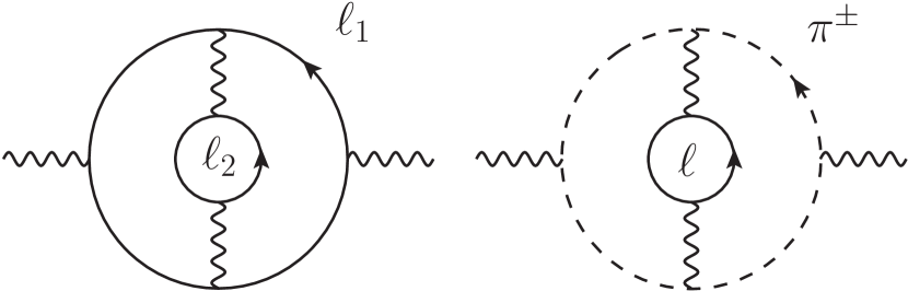
Figure 1: Left: double-bubble topology in QED, for outer lepton $\ell_{1}$ and inner lepton $\ell_{2}$. Right: example for a hadronic manifestation of the same topology with quarks in the outer loop and lepton $\ell$ in the inner loop. The opposite case (lepton outer loop, hadrons inner loop) is irrelevant numerically, see main text. Similar diagrams with inner-bubble insertions on the same side of the outer loop are not shown, nor are additional diagrams in scalar QED.

QED.—The vacuum polarization (VP) diagrams in Fig. 1 produce a contribution to $a_{\mu}$ via

$$a_{\mu}=\frac{\alpha}{\pi}\int_{0}^{1}dx(1-x)\bar{\Pi}(s_{x}),\quad s_{x}=-\frac{x^{2}m_{\mu}^{2}}{1-x},$$ (4)

where $\bar{\Pi}(s)$ is the renormalized scalar VP function in the sign convention that the fine-structure constant runs as $\alpha(s)=\alpha(0)/(1-\bar{\Pi}(s))$. We will evaluate Eq. (4) via the dispersion relation

$$\bar{\Pi}(s)=\frac{s}{\pi}\int_{s_{\text{thr}}}^{\infty}ds^{\prime}\frac{\text{Im}\,\Pi(s^{\prime})}{s^{\prime}(s^{\prime}-s)},$$ (5)

since $\text{Im}\,\Pi(s)$ can be directly related to the cuts of the diagrams. To be explicit, one has the relation

$$\text{Im}\,\Pi(s)=-\frac{\alpha}{3}R(s),$$ (6)

where the $R$-ratio is defined as

$$R(s)=\frac{\sigma(e^{+}e^{-}\to\text{hadrons})}{\sigma_{0}},\qquad\sigma_{0}=\frac{4\pi\alpha^{2}}{3s}.$$ (7)

Of course, the same formula also works for leptonic final states, so that the left diagram in Fig. 1 can be reconstructed from the $\ell_{1}^{+}\ell_{1}^{-}$ cut, starting at $s_{\text{thr}}=4m_{\ell_{1}}^{2}$, and the $\ell_{1}^{+}\ell_{1}^{-}\ell_{2}^{+}\ell_{2}^{-}$ cut, starting at $s_{\text{thr}}=(2m_{\ell_{1}}+2m_{\ell_{2}})^{2}$. As a first step, we work out the results for the cases $\{\ell_{1}\ell_{2}\}=\{ee,\mu e,e\mu\}$, since the separation into the two cuts, referred to as virtual and real contributions, respectively, will allow us to draw first conclusions on the hadronic case.

To this end, we introduce the notation

$$R^{(2)}_{\ell_{1}\ell_{2}}(s)=\bigg{(}\frac{\alpha}{\pi}\bigg{)}^{2}\big{(}\rho^{V}_{\ell_{1}\ell_{2}}(s)+\rho^{R}_{\ell_{1}\ell_{2}}(s)\big{)}$$ (8)

for the two-loop contribution to $R(s)$ and separate the scaling in $\alpha/\pi$ to obtain the spectral functions $\rho^{V,R}_{\ell_{1}\ell_{2}}$ for the virtual and real parts.

The virtual spectral function can be calculated by yet another dispersion relation,

$$\rho^{V}_{\ell_{1}\ell_{2}}(s) =(3-\beta_{1}^{2})\beta_{1}\text{Re}\,F_{1}^{\ell_{1}\ell_{2}}(s)+3\beta_{1}\text{Re}\,F_{2}^{\ell_{1}\ell_{2}}(s),$$

$$F_{i}^{\ell_{1}\ell_{2}}(s) =\frac{1}{3}\int_{4m_{2}^{2}}^{\infty}\frac{d\lambda^{2}}{\lambda^{2}}F_{i}^{\ell_{1}\lambda}(s,\lambda^{2})R_{\ell_{2}}(\lambda^{2}),$$ (9)

where

$$R_{\ell}(s)=\sqrt{1-\frac{4m_{\ell}^{2}}{s}}\bigg{(}1+\frac{2m_{\ell}^{2}}{s}\bigg{)}$$ (10)

is the spectral function for the inner lepton $\ell_{2}$ and we wrote $m_{i}=m_{\ell_{i}}$ as well as $\beta_{i}=\sqrt{1-4m_{i}^{2}/s}$. The $F_{i}^{\ell_{1}\lambda}(s,\lambda^{2})$ are the one-loop QED Dirac and Pauli form factors, but calculated for a finite photon mass $\lambda$ Hoang et al. (1995a); Hoang and Teubner (1998), see Eq. (A) for the explicit expressions app . The resulting integral representation (Mixed leptonic and hadronic corrections to the anomalous magnetic moment of the muon) works well for $\ell_{1}=\mu$, leading to the result shown in Table 1. For $\ell_{1}=\ell_{2}=e$ one can use the analytic result Teubner (1995); Hoang (1995), reproduced in Eq. (19), while for $\ell_{1}=e$, $\ell_{2}=\mu$ in most of the integration range in Eq. (5) the approximation $m_{1}=0$ is sufficient. The exception is the region very close to threshold, where a double expansion (A) in $\beta_{1}$ and $m_{1}^{2}/\lambda^{2}$ should be used instead. Finally, the known real spectral function from the four-particle cut is given in Eq. (A).

	virtual	real	total	Refs. Aoyama et al. (2012); Nio (2021)
$\ell_{1}=\ell_{2}=e$	$-3.56$	$5.00$	$1.44$	$1.4407623(330)$
$\ell_{1}=\mu,\ell_{2}=e$	$-0.11$	$0.27$	$0.16$	$0.1619701(214)$
$\ell_{1}=e,\ell_{2}=\mu$	$0.02$	$0.002$	$0.02$	$0.0215813(40)$
$\ell=e$	$-0.13$	$0.25$	$0.12$

Table 1: Contributions to $a_{\mu}$ in units of $(\alpha/\pi)^{4}\simeq 2.9\times 10^{-11}$. The upper panel refers to the QED diagrams (left in Fig. 1), the last line to an estimate of the $\pi^{+}\pi^{-}$ contribution in scalar QED (right in Fig. 1). The virtual and real parts correspond to the two- and four-particle cuts, respectively.

The sum of the real and virtual contributions reproduces the total results from Refs. Aoyama et al. (2012); Nio (2021), see Table 1. We see that by far the dominant contribution arises from $\ell_{1}=\ell_{2}=e$, as expected given the additional light loop compared to the other two cases. Moreover, we observe that (i) the configuration with an outer electron and inner muon comes out much smaller than the opposite case and (ii) the cancellation of the leading logarithms is most visible for $\ell_{1}=\ell_{2}=e$, with a milder effect already for $\ell_{1}=\mu$, $\ell_{2}=e$.

Since the muon mass is similar to the hadronic scales, e.g., close to the mass of the pion, these observations provide some first insights for the corresponding diagrams with hadronic degrees of freedom. First, we can ignore the case of on outer electron and inner hadronic loop, since the muon example shows that this configuration contributes only $\lesssim 10^{-12}$ to $a_{\mu}$. Second, virtual corrections will be included in the $e^{+}e^{-}\to\text{hadrons}$ data in LO HVP, unless removed by hand through the application of higher-order radiative corrections or in Monte Carlo simulations. This implies that the only potentially missing effect concerns the real radiation of an $e^{+}e^{-}$ pair together with hadronic states. In the muon case, this effect amounts to $\Delta a_{\mu}\simeq 0.8\times 10^{-11}$, which would be negligible for the time being. To corroborate this estimate, we consider a $\pi^{+}\pi^{-}$ loop in scalar QED, as a realistic example of the hadronic realization of a quark loop, see right diagram in Fig. 1.

Scalar QED.—To estimate the potentially missing hadronic contributions more quantitatively, we consider the $e^{+}e^{-}\to\pi^{+}\pi^{-}$ cross section parameterized via the pion vector form factor $F_{\pi}^{V}(s)$,

$$\sigma(e^{+}e^{-}\to\pi^{+}\pi^{-})=\frac{\pi\alpha^{2}}{3s}\beta_{\pi}^{3}\big{|}F_{\pi}^{V}(s)\big{|}^{2},$$ (11)

with $\beta_{\pi}=\sqrt{1-4M_{\pi}^{2}/s}$, and evaluate the virtual and real corrections in scalar QED. This strategy is analogous to the calculation of $\pi\pi\gamma$ radiative corrections Hoefer et al. (2002); Czyż et al. (2005); Gluza et al. (2003); Bystritskiy et al. (2005) and captures the infrared enhanced effects, for which the pion can be approximated as a point-like particle.

The calculation of the virtual contribution proceeds in analogy to Eq. (Mixed leptonic and hadronic corrections to the anomalous magnetic moment of the muon),

$$\rho_{\pi\ell}^{V}(s) =\frac{1}{2}\beta_{\pi}^{3}\big{|}F_{\pi}^{V}(s)\big{|}^{2}\text{Re}\,F^{\pi\ell}(s),$$

$$F^{\pi\ell}(s) =\frac{1}{3}\int_{4m_{\ell}^{2}}^{\infty}\frac{d\lambda^{2}}{\lambda^{2}}F^{\pi\lambda}(s,\lambda^{2})R_{\ell}(\lambda^{2}),$$ (12)

where the form factor $F^{\pi\lambda}(s,\lambda^{2})$ fulfills the dispersion relation

$$F^{\pi\lambda}(s,\lambda^{2})=\frac{s}{\pi}\int_{4M_{\pi}^{2}}^{\infty}ds^{\prime}\frac{\text{Im}\,F^{\pi\lambda}(s^{\prime},\lambda^{2})}{s^{\prime}(s^{\prime}-s)}.$$ (13)

From the explicit scalar QED calculation we obtain the compact analytic expression

$$F^{\pi\lambda}(s,\lambda^{2}) =-\frac{1}{4\beta}\bigg{[}1+\beta^{2}+\frac{2+\beta^{2}-3\beta^{4}}{4\beta^{2}}l+\frac{(1-\beta^{2})^{2}}{8\beta^{2}}l^{2}\bigg{]}\psi(p,l)-\bigg{[}\frac{1}{2\beta^{2}}+\frac{1+\beta^{2}}{8\beta^{2}}l-\frac{1}{4}\bigg{]}\phi(l)$$

$$-\frac{1}{16\beta^{2}}\bigg{[}1+\beta^{2}+\frac{(1-\beta^{2})^{2}}{2\beta}\log p\bigg{]}l^{2}\log l-\frac{1}{16\beta^{2}}\bigg{[}4-6\beta^{2}+\frac{2+\beta^{2}-3\beta^{4}}{\beta}\log p\bigg{]}l\log l-\frac{(1-\beta^{2})^{2}\log^{2}p}{64\beta^{3}}l^{2}$$

$$+\frac{1}{4}\bigg{[}1-\frac{1-\beta^{2}}{8\beta^{3}}\log p\Big{(}4\beta^{2}+(2+3\beta^{2})\log p\Big{)}\bigg{]}l-\frac{1}{2}\bigg{[}1+\frac{1+\beta^{2}}{2\beta}\log p\bigg{]}\log l-\frac{\log p}{8\beta}(1+\beta^{2})(4+\log p)-1$$

$$+i\pi\Bigg{\{}-\frac{1}{2\beta}\bigg{[}1+\beta^{2}+\frac{1-\beta^{2}}{4}l\bigg{]}+\frac{1}{4\beta}\bigg{[}1+\beta^{2}+\frac{2+\beta^{2}-3\beta^{4}}{4\beta^{2}}l+\frac{(1-\beta^{2})^{2}}{8\beta^{2}}l^{2}\bigg{]}\log\bigg{[}1+\frac{(1-p)^{2}}{lp}\bigg{]}\Bigg{\}},$$ (14)

where $\beta=\beta_{\pi}$, $p=\frac{1-\beta}{1+\beta}$, $l=\lambda^{2}/M_{\pi}^{2}$, and

$$\phi(l) =\begin{cases}\frac{1}{2}\sqrt{l^{2}-4l}\log\frac{l-\sqrt{l^{2}-4l}}{l+\sqrt{l^{2}-4l}}\qquad\text{for}\quad l>4\\ \sqrt{4l-l^{2}}\arctan\frac{\sqrt{4l-l^{2}}}{l}\qquad\text{for}\quad 0<l<4\end{cases},$$

$$\psi(p,l) =\frac{1}{2}\log^{2}\bigg{(}\frac{1}{2}\Big{[}l-2+\sqrt{l^{2}-4l}\Big{]}\bigg{)}+\text{Li}_{2}\bigg{(}1+\frac{p}{2}\Big{[}-2+l+\sqrt{l^{2}-4l}\Big{]}\bigg{)}+\text{Li}_{2}\bigg{(}1+\frac{p}{2}\Big{[}-2+l-\sqrt{l^{2}-4l}\Big{]}\bigg{)}$$

$$+\begin{cases}-\frac{\pi^{2}}{2}+i\pi\log\Big{(}(1-p)^{2}+pl\Big{)}\qquad\text{for}\quad l>4\\ -\frac{3}{2}\pi^{2}+4\pi\arctan\frac{\sqrt{4l-l^{2}}}{l}+2\pi\arctan\frac{2p+l-2}{\sqrt{4l-l^{2}}}\qquad\text{for}\quad 0<l<4\end{cases}.$$ (15)

Similarly, real radiation from the scalar QED subprocess leads to the spectral function

$$\rho^{R}_{\pi\ell}(s) =\frac{4}{3}\big{|}F_{\pi}^{V}(s)\big{|}^{2}\int_{y_{-}}^{y_{+}}dy\int_{z_{-}}^{z_{+}}\frac{dz}{z}\bigg{(}1+\frac{2m_{\ell}^{2}}{sz}\bigg{)}\sqrt{1-\frac{4m_{\ell}^{2}}{sz}}\Bigg{[}\sqrt{1-\frac{4M_{\pi}^{2}}{sy}}\lambda^{1/2}(1,y,z)\Bigg{(}\frac{1}{8}+\frac{\Big{(}\frac{4M_{\pi}^{2}}{s}-1\Big{)}\Big{(}\frac{4M_{\pi}^{2}}{s}-z\Big{)}}{32\big{(}z+\frac{M_{\pi}^{2}}{sy}\lambda(1,y,z)\big{)}}\Bigg{)}$$

$$+\frac{\frac{16M_{\pi}^{4}}{s^{2}}-\frac{4M_{\pi}^{2}}{s}(2y+z+1)+2y(z+1)+z}{16(y-z-1)}\log\frac{1-y+z-\sqrt{1-\frac{4M_{\pi}^{2}}{sy}}\lambda^{1/2}(1,y,z)}{1-y+z+\sqrt{1-\frac{4M_{\pi}^{2}}{sy}}\lambda^{1/2}(1,y,z)}\Bigg{]},$$ (16)

where $\lambda(x,y,z)=x^{2}+y^{2}+z^{2}-2(xy+xz+yz)$ and

$$y_{-} =\frac{4M_{\pi}^{2}}{s}, y_{+} =\bigg{(}1-\frac{2m_{\ell}}{\sqrt{s}}\bigg{)}^{2},$$

$$z_{-} =\frac{4m_{\ell}^{2}}{s}, z_{+} =\big{(}1-\sqrt{y}\big{)}^{2}.$$ (17)

Both $F^{\pi\lambda}(s,\lambda^{2})$ and $\rho^{R}_{\pi\ell}(s)$ are new results.

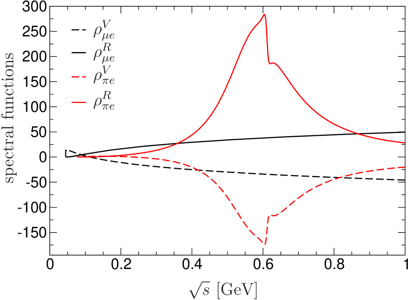
Figure 2: Spectral functions for an inner electron and an outer muon or pion. The figure illustrates how the larger fermionic spectral functions close to threshold and for large $s$ are compensated by the $\rho(770)$ peak in between.

The numerical evaluation gives the result in the last line of Table 1, supporting the conclusions already indicated by the muon example: again, the contribution from the real radiation of $e^{+}e^{-}$ pairs together with final-state $\pi^{+}\pi^{-}$ corresponds to an effect in $a_{\mu}$ of less than $1\times 10^{-11}$. We stress that, while the muon loop is expected to produce results similar to hadronic degrees of freedom given the scales involved, the extent to which the effects in $a_{\mu}$ agree is largely coincidental. As shown in Fig. 2, the fermionic spectral functions tend to be larger near threshold (due to the $P$-wave suppression of the $\pi^{+}\pi^{-}$ channel) and for large $s$ (where $F_{\pi}^{V}\simeq 1/s$ leads to a suppression), which is then compensated by the $\rho(770)$ peak at intermediate energies.

Conclusions.—In this Letter we addressed a missing class of hadronic corrections to the anomalous magnetic moment of the muon at $\mathcal{O}(\alpha^{4})$, represented by the double-bubble topologies shown in Fig. 1. As a first step we reproduced the QED configurations involving electron loops by means of the two- and four-particle cuts of these diagrams, and showed that indeed the known results are recovered when adding the virtual and real contributions. In particular, configurations in which the inner loop does not correspond to an electron prove negligible.

Since virtual corrections should be included in the measured $e^{+}e^{-}\to\text{hadrons}$ cross section, we concluded that the only potentially missed contribution could originate from hadronic final states accompanied by $e^{+}e^{-}$ pair emission. To estimate this effect, we argued that the case with an outer muon should provide a first indication, and then calculated the analog in scalar QED for a charged-pion loop. Both results are remarkably close, albeit to a large extent by coincidence, see Fig. 2, and translate to an effect in $a_{\mu}$ of $\lesssim 1\times 10^{-11}$. One would thus need a significant enhancement due to experimental cuts or misidentification of $e^{+}e^{-}$ pairs to produce a relevant effect. It might be interesting to verify in experimental analyses that indeed no enhanced effects from $e^{+}e^{-}$ radiation can occur, but absent such a scenario we conclude that this class of mixed leptonic and hadronic corrections is negligible at the level required for the final precision of the Fermilab $g-2$ experiment.

Acknowledgments.—We thank Makiko Nio for providing the flavor breakdown of the results from Ref. Aoyama et al. (2012), and acknowledge valuable discussions at the workshop Abbiendi et al. (2022). Financial support by the SNSF under Project No. PCEFP2_181117 (M.H.) and the STFC Consolidated Grant ST/T000988/1 (T.T.) is gratefully acknowledged.

Appendix A QED spectral functions

The QED form factors for finite $\lambda^{2}$ are

$$F_{1}^{\ell\lambda} =-\frac{1}{4\beta}\bigg{[}1+\beta^{2}+\frac{1-\beta^{2}}{\beta^{2}}l\bigg{(}1+\frac{(3-2\beta^{2})(1-\beta^{2})}{8\beta^{2}}l\bigg{)}\bigg{]}\psi(p,l)+\bigg{[}\frac{-1+2\beta^{2}}{2\beta^{2}}+\frac{-3+7\beta^{2}+2\beta^{4}}{8\beta^{4}}l+\frac{3}{l-4}\bigg{]}\phi(l)$$

$$+\frac{1}{16\beta^{4}}\bigg{[}-3+7\beta^{2}+2\beta^{4}+\frac{(1-\beta^{2})^{2}(-3+2\beta^{2})}{2\beta}\log p\bigg{]}l^{2}\log l-\frac{1}{2\beta^{2}}\bigg{[}1+\frac{1-\beta^{2}}{2\beta}\log p\bigg{]}l\log l$$

$$-\bigg{[}\frac{1}{2}+\frac{1+\beta^{2}}{4\beta}\log p\bigg{]}\log l+\frac{(1-\beta^{2})^{2}(-3+2\beta^{2})\log^{2}p}{64\beta^{5}}l^{2}-\frac{1}{4\beta^{2}}\bigg{[}1+2\beta^{2}+\frac{1-\beta^{2}}{2\beta}\log p\Big{(}3-2\beta^{2}+\log p\Big{)}\bigg{]}l$$

$$-\frac{\log p}{8\beta}\bigg{[}2(1+2\beta^{2})+(1+\beta^{2})\log p\bigg{]}-1$$

$$+i\pi\Bigg{\{}-\frac{1+2\beta^{2}}{4\beta}+\frac{(1-\beta^{2})(-3+2\beta^{2})}{8\beta^{3}}l+\frac{1}{4\beta}\bigg{[}1+\beta^{2}+\frac{1-\beta^{2}}{\beta^{2}}l+\frac{(3-2\beta^{2})(1-\beta^{2})^{2}}{8\beta^{4}}l^{2}\bigg{]}\log\bigg{[}1+\frac{(1-p)^{2}}{lp}\bigg{]}\Bigg{\}},$$

$$F_{2}^{\ell\lambda} =\frac{(1-\beta^{2})^{2}}{4\beta^{3}}\bigg{[}1+\frac{3(1-\beta^{2})}{8\beta^{2}}l\bigg{]}l\,\psi(p,l)+\frac{1-\beta^{2}}{2\beta^{2}}\bigg{[}1+\frac{3-5\beta^{2}}{4\beta^{2}}l\bigg{]}\phi(l)$$

$$+\frac{(1+\beta)^{2}(1-\beta^{2})}{16\beta^{4}}\bigg{[}\frac{3-5\beta^{2}}{(1+\beta)^{2}}+\frac{3(1-\beta)^{2}}{2\beta}\log p\bigg{]}l^{2}\log l+\frac{1-\beta^{2}}{2\beta^{2}}\bigg{[}1+\frac{1-\beta^{2}}{2\beta}\log p\bigg{]}l\log l+\frac{3(1-\beta^{2})^{3}}{64\beta^{5}}l^{2}\log^{2}p$$

$$+\frac{1-\beta^{2}}{4\beta^{2}}\bigg{[}1+\frac{1-\beta^{2}}{2\beta}\log p(3+\log p)\bigg{]}l+\frac{1-\beta^{2}}{4\beta}\log p$$

$$+i\pi\Bigg{\{}\frac{1-\beta^{2}}{4\beta}+\frac{3(1-\beta^{2})^{2}}{8\beta^{3}}l-\frac{(1-\beta^{2})^{2}}{4\beta^{3}}\bigg{[}1+\frac{3(1-\beta^{2})}{8\beta^{2}}l\bigg{]}l\,\log\bigg{[}1+\frac{(1-p)^{2}}{lp}\bigg{]}\Bigg{\}},$$ (18)

where $\beta=\sqrt{1-\frac{4m_{\ell}^{2}}{s}}$, $p=\frac{1-\beta}{1+\beta}$, $l=\lambda^{2}/m_{\ell}^{2}$, and $\phi(l)$, $\psi(p,l)$ as in Eq. (Mixed leptonic and hadronic corrections to the anomalous magnetic moment of the muon). In the equal-mass case $\ell_{1}=\ell_{2}=\ell$ also compact expressions for the integral (Mixed leptonic and hadronic corrections to the anomalous magnetic moment of the muon) exist Teubner (1995); Hoang (1995),

$$\text{Re}\,F_{1}^{\ell\ell} =\frac{1}{12\beta^{2}}\Bigg{[}\frac{(2\beta^{2}-1)(9-6\beta^{2}+5\beta^{4})}{24\beta^{3}}\log^{3}p+\frac{31-23\beta^{2}+30\beta^{4}}{12\beta^{2}}\log^{2}p$$ (19)

$$+\bigg{(}\frac{267-238\beta^{2}+236\beta^{4}}{18\beta}+\frac{(1-2\beta^{2})(9-6\beta^{2}+5\beta^{4})\zeta(2)}{2\beta^{3}}\bigg{)}\log p+\frac{(9-21\beta^{2}-10\beta^{4})\zeta(2)}{\beta^{2}}+\frac{147+236\beta^{2}}{9}\Bigg{]},$$

$$\text{Re}\,F_{2}^{\ell\ell} =\frac{1-\beta^{2}}{4\beta^{2}}\Bigg{[}\frac{(1-\beta^{2})^{2}}{8\beta^{3}}\log^{3}p-\frac{11-9\beta^{2}}{12\beta^{2}}\log^{2}p-\bigg{(}\frac{93-68\beta^{2}}{18\beta}+\frac{3(1-\beta^{2})^{2}\zeta(2)}{2\beta^{3}}\bigg{)}\log p+\frac{(5\beta^{2}-3)\zeta(2)}{\beta^{2}}-\frac{17}{3}\Bigg{]}.$$

In the case $\ell_{1}=e$, $\ell_{2}=\mu$ the approximation $m_{1}=0$ is useful for most of the integration range, leading to

$$\rho^{V}_{\ell_{1}\ell_{2}}\big{|}_{m_{1}=0} =\frac{2}{3}\big{(}1-6x^{2}\big{)}\Big{[}\text{Li}_{3}\big{(}A^{2}\big{)}-\zeta(3)-2\zeta(2)\log A+\frac{2}{3}\log^{3}A\Big{]}+\frac{19+46x}{9}\sqrt{1+4x}\Big{[}\text{Li}_{2}\big{(}A^{2}\big{)}-\zeta(2)+\log^{2}A\Big{]}$$

$$+\frac{5}{36}\bigg{(}\frac{53}{3}+44x\bigg{)}\log x+\frac{3355}{648}+\frac{119}{9}x,\qquad A=\frac{\sqrt{1+4x}-1}{\sqrt{4x}},\qquad x=\frac{m_{2}^{2}}{s},$$ (20)

while close to threshold the following double expansion in $\beta=\beta_{1}$ and $l=\lambda^{2}/m_{1}^{2}$ applies:

$$\text{Re}\,F_{1}^{\ell\lambda} =\frac{1}{10395l}\bigg{[}19635-8085\beta^{2}-8085\beta^{4}-9933\beta^{6}-11517\beta^{8}-12837\beta^{10}-13957\beta^{12}+6930\log l\,\sum\limits_{i=0}^{6}\beta^{2i}\bigg{]}$$

$$+\frac{1}{3780l^{2}}\bigg{[}525(29-5\beta^{2})+14805\beta^{4}+23835\beta^{6}+31857\beta^{8}+39735\beta^{10}+47693\beta^{12}-1260\log l\,\sum_{i=0}^{6}(2i+5)\beta^{2i}\bigg{]}$$

$$+\mathcal{O}\Big{(}\beta^{14}l^{-1}\log l,l^{-3}\log l\Big{)},$$

$$\text{Re}\,F_{2}^{\ell\lambda} =\frac{1}{3780l^{2}}\bigg{[}1785-1050\beta^{2}-6090\beta^{4}-7770\beta^{6}-8778\beta^{8}-9498\beta^{10}-10058\beta^{12}-1260\log l+2520\log l\,\sum_{i=1}^{6}\beta^{2i}\bigg{]}$$

$$+\frac{1}{3l}+\mathcal{O}\Big{(}\beta^{14}l^{-2}\log l,l^{-3}\log l\Big{)}.$$ (21)

The four-particle cut leads to the spectral function

$$\rho^{R}_{\ell_{1}\ell_{2}} =\frac{4}{3}\int_{y_{-}}^{y_{+}}dy\int_{z_{-}}^{z_{+}}\frac{dz}{z}\bigg{(}1+\frac{2m_{2}^{2}}{sz}\bigg{)}\sqrt{1-\frac{4m_{2}^{2}}{sz}}\Bigg{[}\sqrt{1-\frac{4m_{1}^{2}}{sy}}\lambda^{1/2}(1,y,z)\Bigg{(}\frac{\frac{2m_{1}^{2}}{s}+\frac{4m_{1}^{4}}{s^{2}}+\Big{(}1+\frac{2m_{1}^{2}}{s}\Big{)}z}{\Big{(}1-\frac{4m_{1}^{2}}{sy}\Big{)}\lambda(1,y,z)-(1-y+z)^{2}}-\frac{1}{4}\Bigg{)}$$

$$+\frac{\frac{2m_{1}^{4}}{s^{2}}+\frac{m_{1}^{2}}{s}(1-y+z)-\frac{1}{4}(1-y+z)^{2}-\frac{1}{2}(1+z)y}{1-y+z}\log\frac{1-y+z-\sqrt{1-\frac{4m_{1}^{2}}{sy}}\lambda^{1/2}(1,y,z)}{1-y+z+\sqrt{1-\frac{4m_{1}^{2}}{sy}}\lambda^{1/2}(1,y,z)}\Bigg{]},$$ (22)

where

$$y_{-}=\frac{4m_{1}^{2}}{s},\qquad y_{+}=\bigg{(}1-\frac{2m_{2}}{\sqrt{s}}\bigg{)}^{2},\qquad z_{-}=\frac{4m_{2}^{2}}{s},\qquad z_{+}=\big{(}1-\sqrt{y}\big{)}^{2}.$$ (23)

References

• Aoyama et al. (2020) T. Aoyama et al., Phys. Rept. 887, 1 (2020), eprint 2006.04822.
• Aoyama et al. (2012) T. Aoyama, M. Hayakawa, T. Kinoshita, and M. Nio, Phys. Rev. Lett. 109, 111808 (2012), eprint 1205.5370.
• Aoyama et al. (2019) T. Aoyama, T. Kinoshita, and M. Nio, Atoms 7, 28 (2019).
• Czarnecki et al. (2003) A. Czarnecki, W. J. Marciano, and A. Vainshtein, Phys. Rev. D 67, 073006 (2003), [Erratum: Phys. Rev. D 73, 119901 (2006)], eprint hep-ph/0212229.
• Gnendiger et al. (2013) C. Gnendiger, D. Stöckinger, and H. Stöckinger-Kim, Phys. Rev. D 88, 053005 (2013), eprint 1306.5546.
• Davier et al. (2017) M. Davier, A. Hoecker, B. Malaescu, and Z. Zhang, Eur. Phys. J. C 77, 827 (2017), eprint 1706.09436.
• Keshavarzi et al. (2018) A. Keshavarzi, D. Nomura, and T. Teubner, Phys. Rev. D 97, 114025 (2018), eprint 1802.02995.
• Colangelo et al. (2019) G. Colangelo, M. Hoferichter, and P. Stoffer, JHEP 02, 006 (2019), eprint 1810.00007.
• Hoferichter et al. (2019) M. Hoferichter, B.-L. Hoid, and B. Kubis, JHEP 08, 137 (2019), eprint 1907.01556.
• Davier et al. (2020) M. Davier, A. Hoecker, B. Malaescu, and Z. Zhang, Eur. Phys. J. C 80, 241 (2020), [Erratum: Eur. Phys. J. C 80, 410 (2020)], eprint 1908.00921.
• Keshavarzi et al. (2020a) A. Keshavarzi, D. Nomura, and T. Teubner, Phys. Rev. D 101, 014029 (2020a), eprint 1911.00367.
• Hoid et al. (2020) B.-L. Hoid, M. Hoferichter, and B. Kubis, Eur. Phys. J. C 80, 988 (2020), eprint 2007.12696.
• Kurz et al. (2014a) A. Kurz, T. Liu, P. Marquard, and M. Steinhauser, Phys. Lett. B 734, 144 (2014a), eprint 1403.6400.
• Melnikov and Vainshtein (2004) K. Melnikov and A. Vainshtein, Phys. Rev. D 70, 113006 (2004), eprint hep-ph/0312226.
• Colangelo et al. (2014a) G. Colangelo, M. Hoferichter, M. Procura, and P. Stoffer, JHEP 09, 091 (2014a), eprint 1402.7081.
• Colangelo et al. (2014b) G. Colangelo, M. Hoferichter, B. Kubis, M. Procura, and P. Stoffer, Phys. Lett. B 738, 6 (2014b), eprint 1408.2517.
• Colangelo et al. (2015) G. Colangelo, M. Hoferichter, M. Procura, and P. Stoffer, JHEP 09, 074 (2015), eprint 1506.01386.
• Masjuan and Sánchez-Puertas (2017) P. Masjuan and P. Sánchez-Puertas, Phys. Rev. D 95, 054026 (2017), eprint 1701.05829.
• Colangelo et al. (2017a) G. Colangelo, M. Hoferichter, M. Procura, and P. Stoffer, Phys. Rev. Lett. 118, 232001 (2017a), eprint 1701.06554.
• Colangelo et al. (2017b) G. Colangelo, M. Hoferichter, M. Procura, and P. Stoffer, JHEP 04, 161 (2017b), eprint 1702.07347.
• Hoferichter et al. (2018a) M. Hoferichter, B.-L. Hoid, B. Kubis, S. Leupold, and S. P. Schneider, Phys. Rev. Lett. 121, 112002 (2018a), eprint 1805.01471.
• Hoferichter et al. (2018b) M. Hoferichter, B.-L. Hoid, B. Kubis, S. Leupold, and S. P. Schneider, JHEP 10, 141 (2018b), eprint 1808.04823.
• Gérardin et al. (2019) A. Gérardin, H. B. Meyer, and A. Nyffeler, Phys. Rev. D 100, 034520 (2019), eprint 1903.09471.
• Bijnens et al. (2019) J. Bijnens, N. Hermansson-Truedsson, and A. Rodríguez-Sánchez, Phys. Lett. B 798, 134994 (2019), eprint 1908.03331.
• Colangelo et al. (2020a) G. Colangelo, F. Hagelstein, M. Hoferichter, L. Laub, and P. Stoffer, Phys. Rev. D 101, 051501 (2020a), eprint 1910.11881.
• Colangelo et al. (2020b) G. Colangelo, F. Hagelstein, M. Hoferichter, L. Laub, and P. Stoffer, JHEP 03, 101 (2020b), eprint 1910.13432.
• Blum et al. (2020) T. Blum, N. Christ, M. Hayakawa, T. Izubuchi, L. Jin, C. Jung, and C. Lehner, Phys. Rev. Lett. 124, 132002 (2020), eprint 1911.08123.
• Colangelo et al. (2014c) G. Colangelo, M. Hoferichter, A. Nyffeler, M. Passera, and P. Stoffer, Phys. Lett. B 735, 90 (2014c), eprint 1403.7512.
• Calmet et al. (1976) J. Calmet, S. Narison, M. Perrottet, and E. de Rafael, Phys. Lett. B 61, 283 (1976).
• Pauk and Vanderhaeghen (2014) V. Pauk and M. Vanderhaeghen, Eur. Phys. J. C 74, 3008 (2014), eprint 1401.0832.
• Danilkin and Vanderhaeghen (2017) I. Danilkin and M. Vanderhaeghen, Phys. Rev. D 95, 014019 (2017), eprint 1611.04646.
• Jegerlehner (2017) F. Jegerlehner, Springer Tracts Mod. Phys. 274, 1 (2017).
• Knecht et al. (2018) M. Knecht, S. Narison, A. Rabemananjara, and D. Rabetiarivony, Phys. Lett. B 787, 111 (2018), eprint 1808.03848.
• Eichmann et al. (2020) G. Eichmann, C. S. Fischer, and R. Williams, Phys. Rev. D 101, 054015 (2020), eprint 1910.06795.
• Roig and Sánchez-Puertas (2020) P. Roig and P. Sánchez-Puertas, Phys. Rev. D 101, 074019 (2020), eprint 1910.02881.
• Borsanyi et al. (2021) S. Borsanyi et al., Nature 593, 51 (2021), eprint 2002.12347.
• Lehner and Meyer (2020) C. Lehner and A. S. Meyer, Phys. Rev. D 101, 074515 (2020), eprint 2003.04177.
• Crivellin et al. (2020) A. Crivellin, M. Hoferichter, C. A. Manzari, and M. Montull, Phys. Rev. Lett. 125, 091801 (2020), eprint 2003.04886.
• Keshavarzi et al. (2020b) A. Keshavarzi, W. J. Marciano, M. Passera, and A. Sirlin, Phys. Rev. D 102, 033002 (2020b), eprint 2006.12666.
• Malaescu and Schott (2021) B. Malaescu and M. Schott, Eur. Phys. J. C 81, 46 (2021), eprint 2008.08107.
• Colangelo et al. (2021a) G. Colangelo, M. Hoferichter, and P. Stoffer, Phys. Lett. B 814, 136073 (2021a), eprint 2010.07943.
• Hoferichter and Stoffer (2020) M. Hoferichter and P. Stoffer, JHEP 05, 159 (2020), eprint 2004.06127.
• Lüdtke and Procura (2020) J. Lüdtke and M. Procura, Eur. Phys. J. C 80, 1108 (2020), eprint 2006.00007.
• Bijnens et al. (2020) J. Bijnens, N. Hermansson-Truedsson, L. Laub, and A. Rodríguez-Sánchez, JHEP 10, 203 (2020), eprint 2008.13487.
• Bijnens et al. (2021) J. Bijnens, N. Hermansson-Truedsson, L. Laub, and A. Rodríguez-Sánchez, JHEP 04, 240 (2021), eprint 2101.09169.
• Zanke et al. (2021) M. Zanke, M. Hoferichter, and B. Kubis, JHEP 07, 106 (2021), eprint 2103.09829.
• Chao et al. (2021) E.-H. Chao, R. J. Hudspith, A. Gérardin, J. R. Green, H. B. Meyer, and K. Ottnad, Eur. Phys. J. C 81, 651 (2021), eprint 2104.02632.
• Danilkin et al. (2021) I. Danilkin, M. Hoferichter, and P. Stoffer, Phys. Lett. B 820, 136502 (2021), eprint 2105.01666.
• Colangelo et al. (2021b) G. Colangelo, F. Hagelstein, M. Hoferichter, L. Laub, and P. Stoffer, Eur. Phys. J. C 81, 702 (2021b), eprint 2106.13222.
• Bennett et al. (2006) G. W. Bennett et al. (Muon $g-2$), Phys. Rev. D 73, 072003 (2006), eprint hep-ex/0602035.
• Abi et al. (2021) B. Abi et al. (Muon $g-2$), Phys. Rev. Lett. 126, 141801 (2021), eprint 2104.03281.
• Albahri et al. (2021a) T. Albahri et al. (Muon $g-2$), Phys. Rev. D 103, 072002 (2021a), eprint 2104.03247.
• Albahri et al. (2021b) T. Albahri et al. (Muon $g-2$), Phys. Rev. A 103, 042208 (2021b), eprint 2104.03201.
• Albahri et al. (2021c) T. Albahri et al. (Muon $g-2$), Phys. Rev. Accel. Beams 24, 044002 (2021c), eprint 2104.03240.
• Grange et al. (2015) J. Grange et al. (Muon $g-2$) (2015), eprint 1501.06858.
• Abe et al. (2019) M. Abe et al., PTEP 2019, 053C02 (2019), eprint 1901.03047.
• Aiba et al. (2021) M. Aiba et al. (2021), eprint 2111.05788.
• Teubner (1995) T. Teubner (1995), PhD thesis, Karlsruhe.
• Hoang (1995) A. H. Hoang (1995), PhD thesis, Karlsruhe.
• Hoang et al. (1994a) A. H. Hoang, M. Jeżabek, J. H. Kühn, and T. Teubner, Phys. Lett. B 325, 495 (1994a), [Erratum: Phys. Lett. B 327, 439 (1994)], eprint hep-ph/9401283.
• Hoang et al. (1994b) A. H. Hoang, M. Jeżabek, J. H. Kühn, and T. Teubner, Phys. Lett. B 338, 330 (1994b), eprint hep-ph/9407338.
• Hoang et al. (1995a) A. H. Hoang, J. H. Kühn, and T. Teubner, Nucl. Phys. B 452, 173 (1995a), eprint hep-ph/9505262.
• Hoang et al. (1995b) A. H. Hoang, J. H. Kühn, and T. Teubner, Nucl. Phys. B 455, 3 (1995b), eprint hep-ph/9507255.
• Brodsky et al. (1995) S. J. Brodsky, A. H. Hoang, J. H. Kühn, and T. Teubner, Phys. Lett. B 359, 355 (1995), eprint hep-ph/9508274.
• Chetyrkin et al. (1996) K. G. Chetyrkin, A. H. Hoang, J. H. Kühn, M. Steinhauser, and T. Teubner, Phys. Lett. B 384, 233 (1996), eprint hep-ph/9603313.
• Hoang and Teubner (1998) A. H. Hoang and T. Teubner, Nucl. Phys. B 519, 285 (1998), eprint hep-ph/9707496.
• (67) The appendix summarizes the QED spectral functions.
• Nio (2021) M. Nio (2021), private communication.
• Laporta (1993) S. Laporta, Phys. Lett. B 312, 495 (1993), eprint hep-ph/9306324.
• Kinoshita and Nio (2006) T. Kinoshita and M. Nio, Phys. Rev. D 73, 013003 (2006), eprint hep-ph/0507249.
• Kataev (2012) A. L. Kataev, Phys. Rev. D 86, 013010 (2012), eprint 1205.6191.
• Kurz et al. (2014b) A. Kurz, T. Liu, P. Marquard, and M. Steinhauser, Nucl. Phys. B 879, 1 (2014b), eprint 1311.2471.
• Kurz et al. (2015) A. Kurz, T. Liu, P. Marquard, A. V. Smirnov, V. A. Smirnov, and M. Steinhauser, Phys. Rev. D 92, 073019 (2015), eprint 1508.00901.
• Kurz et al. (2016) A. Kurz, T. Liu, P. Marquard, A. Smirnov, V. Smirnov, and M. Steinhauser, Phys. Rev. D 93, 053017 (2016), eprint 1602.02785.
• Hoefer et al. (2002) A. Hoefer, J. Gluza, and F. Jegerlehner, Eur. Phys. J. C 24, 51 (2002), eprint hep-ph/0107154.
• Czyż et al. (2005) H. Czyż, A. Grzelińska, J. H. Kühn, and G. Rodrigo, Eur. Phys. J. C 39, 411 (2005), eprint hep-ph/0404078.
• Gluza et al. (2003) J. Gluza, A. Hoefer, S. Jadach, and F. Jegerlehner, Eur. Phys. J. C 28, 261 (2003), eprint hep-ph/0212386.
• Bystritskiy et al. (2005) Y. M. Bystritskiy, E. A. Kuraev, G. V. Fedotovich, and F. V. Ignatov, Phys. Rev. D 72, 114019 (2005), eprint hep-ph/0505236.
• Abbiendi et al. (2022) G. Abbiendi et al. (2022), eprint 2201.12102.