Dynamical approximations for composite quantum systems: Assessment of error estimates for a separable ansatz

Abstract.

Numerical studies are presented to assess error estimates for a separable (Hartree) approximation for dynamically evolving composite quantum systems which exhibit distinct scales defined by their mass and frequency ratios. The relevant error estimates were formally described in our previous work [I. Burghardt, R. Carles, C. Fermanian Kammerer, B. Lasorne, C. Lasser, J. Phys. A. 54, 414002 (2021)]. Specifically, we consider a representative two-dimensional tunneling system where a double well and a harmonic coordinate are cubically coupled. The time-dependent Hartree approximation is compared with a fully correlated solution, for different parameter regimes. The impact of the coupling and the resulting correlations are quantitatively assessed in terms of a time-dependent reaction probability along the tunneling coordinate. We show that the numerical error is correctly predicted on moderate time scales by a theoretically derived error estimate.

1. Introduction

The time-dependent Hartree (TDH) approximation, also termed time-dependent self-consistent field method [1, 2, 3], which represents the time propagation of composite quantum systems within a separable (Hartree) approximation, is ubiquitous in quantum and classical statistical physics. This approximation is based on a mean-field description and often works well if the relevant subspaces are weakly coupled, and if a separation of scales is given due to disparities in masses and/or frequencies. The TDH approximation is also a natural starting point for including correlations in terms of sums of products, i.e., using a correlated multiconfigurational (MC) ansatz that leads to a Multiconfiguration Time-Dependent Hartree (MCTDH) [4, 5] form of the wavefunction. Related tensor representations of multidimensional wavefunctions are cast in the form of matrix product states [6, 7]. A variational setting [5, 8] is generally employed to obtain generalized, multiconfigurational mean-field equations for such correlated wavefunctions. The TDH and MCTDH representations can be straightforwardly adapted to fermionic or bosonic systems. In the present context, we refer to distinguishable particles for simplicity.

Despite the importance of the TDH ansatz, an explicit error analysis of this approach is not often reported in the literature. In a recent formal paper [9], we therefore presented error estimates for the time propagation of composite quantum systems within the TDH approximation. We also compared different types of approximate product wavefunctions, i.e., based on Taylor expansion (collocation) or else on the TDH mean-field approach, and we further considered a semiclassical approximation within a quantum-classical type treatment. Such semiclassical, or quantum-classical approximations are especially useful if the system is composite – or structured – in a physical sense such that the subsystems exhibit different time and/or energy scales. In the present paper, we follow up on this previous work and carry out numerical simulations to assess the previously derived error estimates for a realistic, anharmonically coupled system exhibiting a separation of scales defined by the relevant mass and frequency ratios. As in the formal paper mentioned above, the present study is meant to be a first step towards a general analysis of scale separation in the context of multiconfigurational, tensorized wavefunction representations.

Specifically, we consider numerical simulations for a two-dimensional tunneling system where a double-well potential is anharmonically coupled to a harmonic coordinate. As in Ref. [9], a cubic coupling is considered (i.e., linear in the tunneling coordinate and quadratic in the harmonic coordinate). Numerical TDH calculations for different parameter regimes are compared with correlated MCTDH calculations that can be considered as numerically exact for the present system. The impact of the coupling and the resulting correlations are quantitatively assessed in terms of a time-dependent reaction probability along the tunneling coordinate.

A time-dependent error estimate is expressed quantitatively in terms of the relevant parameters of the Hamiltonian, leading to insight into the “small” parameters to be considered to gauge the validity of the TDH approximation. This leads us to question the conventional viewpoint that mass ratios are decisive; indeed, within our present analysis, it is the frequency ratio that is found to play a more important role.

The present study paves the way for a more general treatment including the effects of fluctuations and dissipation, which are expected to have a non-trivial effect on the tunneling dynamics [10, 11].

The paper is organized as follows. Section 2 presents the model Hamiltonian under consideration and gives a detailed account of the relevant parameters and their scaling properties. Section 3 addresses the TDH approximation and Section 4 details the formulation of time-dependent error estimates. Section 5 presents the numerical results and Section 6 concludes.

2. Model system

In line with our previous work [9], we consider a two-dimensional model system which is of system-bath type and exhibits anharmonicities both within the system subspace and in the system-bath coupling. Specifically, a double-well potential is chosen in the system subspace, which is coupled to a harmonic bath coordinate via a cubic (quadratic times linear) coupling term. As pointed out in our previous analysis [9], a cubic coupling is a non-trivial case which is relevant for the description of vibrational dephasing [12, 13] and Fermi resonances [14] in a molecular physics context.

Here and in the following, we adhere to a system-bath terminology despite the low-dimensional nature of the model system, due to the fact that the low-frequency harmonic vibration coupled to the dominant tunneling coordinate essentially acts as a bath mode. From a more rigorous viewpoint, the single bath coordinate under consideration carries non-Markovian effects that emerge from a decomposition of memory effects in terms of effective-mode chains [15, 16]. Following this description, we recently considered a related two-dimensional tunneling system where a single effective bath mode is augmented by a Markovian master equation [17]. Likewise, the present treatment can be augmented such as to yield a full system-bath treatment. However, the purpose of the present work is to investigate dynamical approximations for the effective bath mode that is accounted for explicitly.

From a complementary viewpoint, the present system can be considered as a typical example of multi-dimensional tunneling which is frequently encountered in polyatomic molecular systems [18] and has been extensively investigated, both experimentally and theoretically [19, 20, 21, 22]. Multi-dimensional tunneling involves multiple time scales, resonance effects, vibrational mode selectivity, and non-statistical energy redistribution. The present system, even though comparatively simple, falls into a typical parameter regime of such molecular systems, and will be shown to exhibit some of the features mentioned above, specifically the observation of multiple time scales and the interference of seemingly passive spectator modes with the tunneling process.

2.1. Hamiltonian in physical scaling

In system-bath form, the Hamiltonian is written as follows,

$${\mathcal{H}}=H_{X}+H_{Y}+W(X,Y),$$

with the subspace Hamiltonians

$$H_{X}=-\frac{\hbar^{2}}{2\mu_{1}}\Delta_{X}+V_{1}(X),\qquad\qquad H_{Y}=-\frac{\hbar^{2}}{2\mu_{2}}\Delta_{Y}+V_{2}(Y),$$

where $V_{1}(X)$ corresponds to a double-well potential and $V_{2}(Y)$ is a harmonic form,

$$V_{1}(X)=\frac{1}{2}k^{0}_{1}X^{2}\left(\frac{X}{2L}-1\right)^{2},\qquad\qquad V_{2}(Y)=\frac{1}{2}k^{0}_{2}Y^{2}.$$

The system potential $V_{1}(X)$ represents a symmetric double well with two equivalent minima at $X=0$ and $X=2L$ that can be taken to correspond to the “reactant” vs. “product” in the context of a reactive process [18]. The energy at the barrier $X=L$ amounts to $D_{1}=k_{1}^{0}L^{2}/8$.

The coupling $W(X,Y)$ is given as a cubic term, i.e., linear in $X$ and quadratic in $Y$,

$$W(X,Y)=\frac{1}{2}\eta^{0}XY^{2}.$$

Viewed from a different angle, $V_{2}(Y)$ and $W(X,Y)$ can be combined into an effective potential for the $Y$ coordinate,

$$V_{2}^{\rm eff}=V_{2}(Y)+W(X,Y)=\frac{1}{2}\left(k^{0}_{2}+\eta^{0}X\right)Y^{2}\equiv\frac{1}{2}k_{2}(X)Y^{2},$$

whose curvature is $X$-dependent, i.e., the local force constant is given as $k_{2}(X)=k_{2}^{0}+\eta^{0}X$. We denote the ratio of the curvature along $Y$, taken at the product versus reactant minima in $X$, by

(1) $$\alpha=\frac{k_{2}(X=2L)}{k_{2}(X=0)}=1+2\frac{\eta^{0}}{k_{2}^{0}}L.$$

The reduced parameter $\alpha$ gives a direct measure of the relative coupling strength upon characterizing how much the local curvature for $Y$ changes as $X$ varies from $0$ (reactant minimum) to $2L$ (product minimum).

Yet from a different perspective, an adiabatic regime can be considered whose “fast” subsystem ($X$) coordinate is coupled to a “slow” bath ($Y$) coordinate. An effective subsystem Hamiltonian can then be defined as follows,

$$H_{1}^{\rm eff}=-\frac{\hbar^{2}}{2\mu_{1}}\Delta_{X}+V(X,Y)\qquad V(X,Y)=V_{1}(X)+V_{2}(Y)+W(X,Y).$$

Which perspective is most appropriate depends on the physical time scales under study, as will be detailed below.

Finally, we note that the extension of this model to multivariate coordinates $X$ and $Y$ is straightforward, such that the present model is suitable to address general multidimensional tunneling situations.

2.2. Parameter choice

In the present work, we exclusively consider negative values of the coupling parameter $\eta^{0}$ such that the curvature ratio defined in Eq. (1) satisfies $\alpha<1$. This ensures that the ground eigenstate of the full $(X,Y)$-system is localized around the product well ($X=2L>0$), while nonstationary dynamics will start from an initial condition (or, in mathematical language, an initial datum) localized around the reactant well ($X=0$). In other words, we reverse localization in order to create an initial nonstationary state.

The cubic coupling potential $W(X,Y)$ has to be handled with some care. It causes the potential energy to be unbounded from below beyond the controllable subquadratic regime. This is likely to induce numerical issues and renders the Hamiltonian ${\mathcal{H}}$ only formally self-adjoint. One might therefore either add a contribution to the potential energy that is quartically confining with respect to $Y$ or multiply the coupling potential with a cut-off function in $X$. Here we have chosen another simple approach: There exists a critical value $X=X_{\mathrm{c}}=\frac{2L}{1-\alpha}>0$ where $k_{2}(X=X_{\mathrm{c}})=0$, which is called a valley-ridge inflection point [23]. Despite its relevance in terms of bifurcation aspects, this is not the situation that we want to address here. A simple cure is to ensure that such a critical point occurs far enough from $X=2L$ that the potential energy at this point, $V(X=X_{\mathrm{c}},Y=0)=V_{1}(X_{\mathrm{c}})$, is large enough compared to the barrier height, $D_{1}=k_{1}^{0}L^{2}/8$. As will be shown below, we choose our reference model such that $\alpha=\frac{1}{3}$ and $X_{\mathrm{c}}=3L$, which implies that $V_{1}(X_{\mathrm{c}})$ is nine times larger than $D_{1}$. The most “precarious” case we considered is $\alpha=\frac{1}{4}$ and $X_{\mathrm{c}}=\frac{8L}{3}$, which implies that we have $V_{1}(X_{\mathrm{c}})=\frac{256}{81}D_{1}\approx 3.2D_{1}$. Such a range of values for the onset of unboundedness in the potential energy seems a priori far enough that our low-energy wavepackets will be vanishing in critical regions, which is what we also observed in practice.

2.3. Representation in scaled coordinates

In order to transform the Hamiltonian to a suitably scaled representation, we introduce the (angular) frequencies and the corresponding natural length scales of the harmonic approximations for $X$ and $Y$ around the origin,

$$\omega_{i}^{0}=\sqrt{k_{i}^{0}/\mu_{i}},\quad a_{i}^{0}=\sqrt{\hbar/(\mu_{i}\omega_{i}^{0})}$$

for $i=1,2$. The corresponding natural energy and time scales are

$$E_{i}^{0}=\frac{\hbar^{2}}{\mu_{i}(a_{i}^{0})^{2}}=k_{i}^{0}(a_{i}^{0})^{2}=\hbar\omega_{i}^{0},\quad t_{i}^{0}=\frac{\hbar}{E_{i}^{0},}.$$

Note that, e.g., $\{\mu_{1},a_{1}^{0},t_{1}^{0}\}$ can serve as a consistent and complete set of mechanical units for all quantities built on powers of [M][L][T], whereby $\hbar$ is numerically equal to unity due to the relationship between the energy unit $E_{1}^{0}$ and the time unit $t_{1}^{0}$ (much as when considering atomic units). In the spirit of semiclassical scaling, we further introduce a typical parameter defined as the square root of the mass ratios,

$$\varepsilon=\sqrt{\frac{\mu_{1}}{\mu_{2}}}.$$

Scaling both coordinates with respect to the natural length scale of the system coordinate, while the bath coordinate is additionally scaled by $\varepsilon$, we set

$$(x,y)=\left(\frac{1}{a_{1}^{0}}X,\frac{1}{a_{1}^{0}\varepsilon}Y\right),\quad\ell=\frac{L}{a_{1}^{0}}.$$

We thus obtain a scaled Hamiltonian

$$\mathcal{H}=E_{1}^{0}H,$$

where the dimensionless part reads

$$H=-\frac{1}{2}\Delta_{x}-\frac{1}{2}\Delta_{y}+v(x,y),$$

with potential energy

$$v(x,y)=v_{1}(x)+v_{2}(y)+w(x,y),$$

with contributions from the system (double well) and the harmonic bath mode

$$v_{1}(x)=\frac{1}{2}x^{2}\left(\frac{x}{2\ell}-1\right)^{2},\quad v_{2}(y)=\frac{1}{2}\varpi^{2}y^{2},$$

where $\varpi=\omega_{2}^{0}/\omega_{1}^{0}$ denotes the frequency ratio of the bath versus the system. The coupling potential $w(x,y)=\frac{1}{2}\eta xy^{2}$ features the rescaled coupling constant

$$\eta=\frac{(a_{1}^{0})^{3}\varepsilon^{2}}{E_{1}^{0}}\,\eta^{0}.$$

Let us denote the physical time $T$ and the rescaled time $t$, where

$$t=\frac{T}{t_{1}^{0}}=\frac{E_{1}^{0}}{\hbar}T.$$

We can absorb both $E_{1}^{0}$ and $\hbar$ into $t_{1}^{0}$ and recast the time-dependent Schrödinger equation,

$$i\hbar\partial_{T}\Psi(T,X,Y)=\mathcal{H}\Psi(T,X,Y),$$

into dimensionless form as

$$i\partial_{t}\psi(t,x,y)=H\psi(t,x,y).$$

We observe that the curvature ratio defined in Eq. (1) is invariant under the performed linear coordinate scaling. It is related to the coupling constant according to

$$\alpha=1+2\frac{\eta}{\varpi^{2}}\ell\quad\mbox{resp.}\quad\eta=\varpi^{2}\frac{\alpha-1}{2\ell}.$$

The parametrization in terms of the frequency ratio $\varpi$ and the curvature ratio $\alpha$ fully characterizes the interaction of the system and bath via the potential energy. The parameter $\varepsilon$, which represents the mass ratio, only appears indirectly, through the scaling of the $Y$ coordinate and of the $\eta$ parameter.

2.4. Relevant parameter regime and initial data

In view of the numerical simulation results reported below, we now specify the parameter regime which was considered in these simulations. First, a reference model was constructed by the following choice of parameters,

$$\varepsilon_{*}=\frac{1}{4},\ \varpi_{*}=\frac{1}{100},\ \alpha_{*}=\frac{1}{3}.$$

We note that the mass ratio $\varepsilon_{*}$ is moderate, but representative of chemically relevant systems. The frequency ratio $\varpi_{*}$, however, takes a value that is significantly smaller, and will be demonstrated to play an important role in the error estimates to be discussed below.

In the simulations reported below, we explore the dynamics of several variations of this reference model (i.e., cases 0 to 8, while the reference model is denoted case *, see Table 1). Relevant ranges of values for $\alpha$ have been discussed above. As already pointed out, reducing $\alpha$ below values of about $\frac{1}{4}$ could entail issues related to the unboundedness within the space explored by the wavepacket. Note also that “case 3” appeared in our simulations as the most sensitive situation, bringing much larger errors between correlated and uncorrelated descriptions. We suspect that this may reflect the fact that the corresponding time scale of the $Y$ dynamics, now shorter, enters the realm of the time scale of $X$ motion (see Sec. 5 for further discussion), thus making system-bath separability less justified.

In all cases, we chose the initial data to be the approximate Gaussian quasi-coherent ground state localized in the “reactant well”, as illustrated in Fig. 1,

(2) $$\psi(t=0,x,y)=\chi_{0}(x)\phi_{0}(y)=(2\pi)^{-1/2}\varpi^{-1/4}\exp\left(-\frac{1}{2}x^{2}-\frac{\varpi}{2}y^{2}\right).$$

We note that both minima of the potential energy have equal energies, but the zero-point energy is higher in the left reactant well because the curvature for $y$ is higher there. The squeezing in the $y$ direction, due to the $\varpi$ factor in the coherent state width, reflects that this coordinate tends to the classical limit.

Case	$\varepsilon$	$\varpi$	$\alpha$
*	$\varepsilon_{*}$	$\varpi_{*}$	$\alpha_{*}$	reference
0	$\varepsilon_{*}$	$\varpi_{*}$	$1$	no coupling
1	$2\varepsilon_{*}$	$\varpi_{*}$	$\alpha_{*}$
2	$\frac{1}{2}\varepsilon_{*}$	$\varpi_{*}$	$\alpha_{*}$
3	$\varepsilon_{*}$	$4\varpi_{*}$	$\alpha_{*}$	most sensitive
4	$\varepsilon_{*}$	$\frac{1}{4}\varpi_{*}$	$\alpha_{*}$
5	$\varepsilon_{*}$	$\varpi_{*}$	$\frac{3}{4}\alpha_{*}$
6	$\varepsilon_{*}$	$\varpi_{*}$	$\frac{3}{2}\alpha_{*}$
7	$\varepsilon_{*}$	$\varpi_{*}$	$2\alpha_{*}$
8	$\varepsilon_{*}$	$\varpi_{*}$	$\frac{9}{4}\alpha_{*}$

Table 1. Parameter variations of the reference model, that is defined by the values $(\varepsilon_{*},\varpi_{*},\alpha_{*})=(\frac{1}{4},\frac{1}{100},\frac{1}{3})$. These parameters determine the square root of the mass ratio, the frequency ratio, and the curvature ratio, respectively.

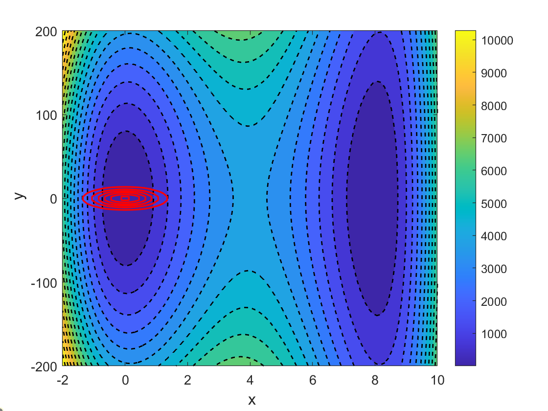
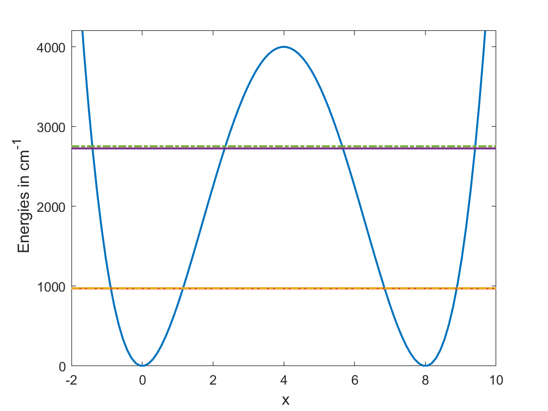
Figure 1. Upper panel: Contour plot of the two-dimensional potential energy surface (reference model *) and coherent-state initial condition according to Eq. (2). As explained in the text, the initial condition corresponds to a non-stationary state localized in the less stable left (“reactant”) well. Lower panel: One-dimensional cut at $y=0$ through the potential and eigenenergies of the ground-state and first excited-state tunneling pairs. The energies are $972$ and $976$ cm^-1 for the ground pair, $2726$ and $2753$ cm^-1 for the excited pair. The splitting of the even and odd energy levels is barely visible on the energy scale set by the potential.

3. Time-dependent Hartree approximation

We compare the numerical solution of the full Schrödinger equation with separable, normalized initial datum

$$\left\{\begin{array}[]{l}i\partial_{t}\psi(t,x,y)=H\psi(t,x,y),\\ \psi(t=0,x,y)=\chi_{0}(x)\phi_{0}(y),\end{array}\right.$$

with the one of the TDH approximation subject to the same initial condition,

$$\left\{\begin{array}[]{l}i\partial_{t}u(t,x,y)=H^{\rm eff}_{u}(t)u(t,x,y),\\ u(t=0,x,y)=\chi_{0}(x)\phi_{0}(y).\end{array}\right.$$

The effective TDH Hamiltonian

$$H^{\rm eff}_{u}(t)=\langle H\rangle_{\phi}^{(x)}(t)+\langle H\rangle_{\chi}^{(y)}(t)-\langle H\rangle_{u}(t),$$

is additive with respect to the coordinates and thus preserves the product structure of the initial datum, i.e., we have

$$u(t,x,y)=a(t)\,\chi(t,x)\,\phi(t,y),$$

where $a(t)$ is a complex number of absolute value one, acting as a suitably chosen gauge factor. The individual product wavefunctions satisfy the coupled equations of motion

$$i\partial_{t}\chi(t,x)=\langle H\rangle_{\phi}(t)\chi(t,x),$$

$$i\partial_{t}\phi(t,y)=\langle H\rangle_{\chi}(t)\phi(t,y),$$

while the gauge factor

$$a(t)=\exp\left(i\int_{0}^{t}\langle H\rangle_{u}(s\,)ds\right)$$

depends on the full energy expectation with respect to the Hartree product. Our system-bath type Hamiltonian is of the form

$$H=H_{x}+H_{y}+w(x,y),$$

with $H_{x}=-\frac{1}{2}\Delta_{x}+v_{1}(x)$ and $H_{y}=-\frac{1}{2}\Delta_{y}+v_{2}(y)$. In this situation, the effective Hartree Hamiltonian is of the form

$$H^{\rm eff}_{u}(t)=H_{x}+H_{y}+w_{u}^{\rm eff}(t,x,y),$$

and differs from the true Hamiltonian only with respect to the effective coupling potential

(5) $$w^{\rm eff}_{u}(t,x,y)=\langle w\rangle_{\phi}(t,x)+\langle w\rangle_{\chi}(t,y)-\langle w\rangle_{u}(t),$$

so the above effective Hamiltonians can be rewritten as

$$\langle H\rangle_{\phi}=H_{x}+\langle w\rangle_{\phi}(t,x),\quad\langle H\rangle_{\chi}=H_{y}+\langle w\rangle_{\chi}(t,y).$$

4. Error estimates

For analyzing the approximation error

$$e(t,x,y)=\psi(t,x,y)-u(t,x,y),$$

we use a standard stability estimate, see Lemma 2 in Ref. [9] Differentiating the error with respect to time we obtain a Schrödinger-type equation

$$\left\{\begin{array}[]{l}i\partial_{t}e(t,x,y)=He(t,x,y)+\Sigma_{u}(t,x,y),\\ e(t=0,x,y)=0,\end{array}\right.$$

with source term

$$\Sigma_{u}(t,x,y) =\left(H-H^{\rm eff}_{u}(t)\right)u(t,x,y)=\left(w(x,y)-w^{\rm eff}_{u}(t,x,y)\right)u(t,x,y).$$

By the variation of constants formula (aka the Duhamel principle), we write the error as a time-integral,

(7) $$e(t,x,y)=\frac{1}{i}\int_{0}^{t}\exp(-iH(t-s))\Sigma_{u}(s,x,y)\,ds.$$

Since the time-evolution associated with the Hamiltonian $H$ is unitary, we now estimate

$$\|e(t)\|_{L^{2}}\leqslant\int_{0}^{t}\|\Sigma_{u}(s)\|_{L^{2}}\,ds$$

for the $L^{2}$-norm of the error.

4.1. Formula for the source term

The cubic coupling potential of our system-bath type Hamiltonian is of product form

$$w(x,y)=w_{1}(x)w_{2}(y).$$

Therefore, the coupling potential of the Hartree approximation, see Eq. (5), takes the special form

$$w^{\rm eff}_{u}(t,x,y)=w_{1}(x)\,\langle w_{2}\rangle_{\phi}(t)+\langle w_{1}\rangle_{\chi}(t)\,w_{2}(y)-\langle w_{1}\rangle_{\chi}(t)\,\langle w_{2}\rangle_{\phi}(t).$$

This implies for the difference of the coupling potentials

$$\delta w_{u}(t,x,y) =w(x,y)-w^{\rm eff}_{u}(t,x,y)$$

$$=\left(w_{1}(x)-\langle w_{1}\rangle_{\chi}(t)\right)\left(w_{2}(y)-\langle w_{2}\rangle_{\phi}(t)\right).$$

We provide a detailed computation of the local-in-time error given in Example 3 of Ref. [9]. We calculate the norm of the source term $\Sigma_{u}(t)=\delta w_{u}(t)u(t)$ according to

$$\|\Sigma_{u}(t)\|_{L^{2}}^{2} =\langle\delta w^{2}\rangle_{u}(t)$$

$$=\left\langle\left[w_{1}(x)-\langle w_{1}\rangle_{\chi}(t)\right]^{2}\right\rangle_{\chi}\,\left\langle\left[w_{2}(y)-\langle w_{2}\rangle_{\phi}(t)\right]^{2}\right\rangle_{\phi}$$

$$=\left(\langle w_{1}^{2}\rangle_{\chi}(t)-\langle w_{1}\rangle_{\chi}(t)^{2}\right)\left(\langle w_{2}^{2}\rangle_{\phi}(t)-\langle w_{2}\rangle_{\phi}(t)^{2}\right).$$

From a probabilistic point of view, we can interpret this formula as the product of the variances of $w_{1}$ and $w_{2}$. Applying this formula to the cubic coupling model, we then obtain the error estimate

$$\|\psi(t)-u(t)\|_{L^{2}}\leqslant\frac{1}{2}|\eta|\int_{0}^{t}\sqrt{\left(\langle x^{2}\rangle_{\chi}(s)-\langle x\rangle_{\chi}^{2}(s)\right)\left(\langle y^{4}\rangle_{\phi}(s)-\langle y^{2}\rangle_{\phi}^{2}(s)\right)}\ ds.$$

4.2. Dimension analysis

This formula is given here in terms of dimensionless energy, space, and time variables; its proof is not affected by scaling considerations, and it directly translates into physical units, $(X,Y,T)$, as

$$\|\Psi(T)-U(T)\|_{L^{2}}\leqslant\frac{1}{2}|\eta^{0}|\times$$

(8) $$\frac{1}{\hbar}\int_{0}^{T}\sqrt{\left(\langle X^{2}\rangle_{X}(S)-\langle X\rangle_{X}^{2}(S)\right)\left(\langle Y^{4}\rangle_{Y}(S)-\langle Y^{2}\rangle_{Y}^{2}(S)\right)}\ dS.$$

From $\eta^{0}=\frac{E_{1}^{0}}{(a_{1}^{0})^{3}\varepsilon^{2}}\,\eta$, recalling $E_{1}^{0}=\frac{\hbar}{t_{1}^{0},}$, and $\eta=\varpi^{2}\varsigma$, where

$$\varsigma=\frac{\alpha-1}{2\ell},$$

the upper bound of the previous estimate can be recast in terms of dimensionless ratios as

$$\frac{\varpi^{2}|\varsigma|}{2t_{1}^{0}}\int_{0}^{T}\sqrt{\frac{\langle X^{2}\rangle_{X}(S)-\langle X\rangle_{X}^{2}(S)}{(a_{1}^{0})^{2}}\frac{\langle Y^{4}\rangle_{Y}(S)-\langle Y^{2}\rangle_{Y}^{2}(S)}{\epsilon^{4}(a_{1}^{0})^{4}}}\ dS$$

$$=\frac{\varpi^{2}|\varsigma|}{2t_{1}^{0}}\int_{0}^{T}\sqrt{\frac{\langle X^{2}\rangle_{X}(S)-\langle X\rangle_{X}^{2}(S)}{(a_{1}^{0})^{2}}\frac{\langle Y^{4}\rangle_{Y}(S)-\langle Y^{2}\rangle_{Y}^{2}(S)}{\varpi^{2}(a_{2}^{0})^{4}}}\ dS$$

$$=\frac{\varpi|\varsigma|}{2t_{1}^{0}}\int_{0}^{T}\sqrt{\frac{\langle X^{2}\rangle_{X}(S)-\langle X\rangle_{X}^{2}(S)}{(a_{1}^{0})^{2}}\frac{\langle Y^{4}\rangle_{Y}(S)-\langle Y^{2}\rangle_{Y}^{2}(S)}{(a_{2}^{0})^{4}}}\ dS,$$

where we used

$$\frac{a_{2}^{0}}{a_{1}^{0}}=\frac{\varepsilon}{\sqrt{\varpi}},$$

and eliminated the somewhat artificial dependence on $\varepsilon$ (noting that different values of $\varepsilon$ only bring homothetic dynamics with respect to $Y$). As a crucial consequence, we removed one power order of $\varpi$ regarding natural orders of magnitude and effective “smallness”.

4.3. Linearization of the upper bound

From an operational point of view, the purpose of rescaling essentially consists in determining relevant orders of magnitude for the values of the various factors entering the relevant formulae. Since we specifically chose initial data to be quasi-coherent states (within a harmonic approximation around the origin), we know that the product of $X$ and $Y^{2}$ standard deviations expressed in their respective natural units satisfy

$$\sqrt{\frac{\langle X^{2}\rangle_{X}(T=0)-\langle X\rangle_{X}^{2}(T=0)}{(a_{1}^{0})^{2}}}\times\sqrt{\frac{\langle Y^{4}\rangle_{Y}(T=0)-\langle Y^{2}\rangle_{Y}^{2}(T=0)}{(a_{2}^{0})^{4}}}=\frac{1}{2},$$

and will not change dramatically over time, which is the incentive for considering a rescaling based on natural units. We can thus further propose a sort of “rough” linear estimate for short times as follows,

(9) $$\|\Psi(T)-U(T)\|_{L^{2}}\lesssim\frac{1}{4}\varpi|\varsigma|\frac{T}{t_{1}^{0}}.$$

where $\lesssim$ here is to be understood as preceding an approximate upper bound. Such an approximation is not aimed at being precise beyond very short times (although we shall see later on that it works surprisingly well at later times) but it presents the great advantage of providing an easy estimate of relevant orders of magnitude before performing any actual propagation. In the present situation, the initial widths along $X$ and $Y$ were chosen to vary as little as possible over time (quasi-coherent initial datum); however, it is not so difficult to make a rough prediction of the time evolution of standard deviations in more general cases (especially oscillatory breathing behaviors with harmonic half periods).

It is worth noticing that we have identified the prefactor $\varpi\varsigma=({\eta}/{\varpi})$ that appears in Eq. (9) as an objective measure of the impact of the coupling on the rate of growth of the error with respect to time. This was not evident at first sight when starting from $\eta^{0}$ as in Eq. (8) written with physical units. It required the dimension analysis presented above so as to get rid of dimensioned quantities and identify what will take values close to unity. The parameter $\varsigma$ only affects the coupling between the system and the bath but can only be varied moderately. In contrast, $\varpi$ can span a large range; however, changing its value affects both the coupling and the relative timescales between system and bath.

We also emphasize that the error in the norm of the difference between two normalized wavefunctions is limited by a strict upper bound, a “maximum maximorum”, which is $\sqrt{2}$ (in the worst and undesired case of strict orthogonality between the solution and its approximation). The intersection of our estimate with this value gives a maximal time of relevance for the estimate, but also a predictive rough order of magnitude of the time beyond which an uncorrelated approximation is definitely at risk.

5. Results and discussion

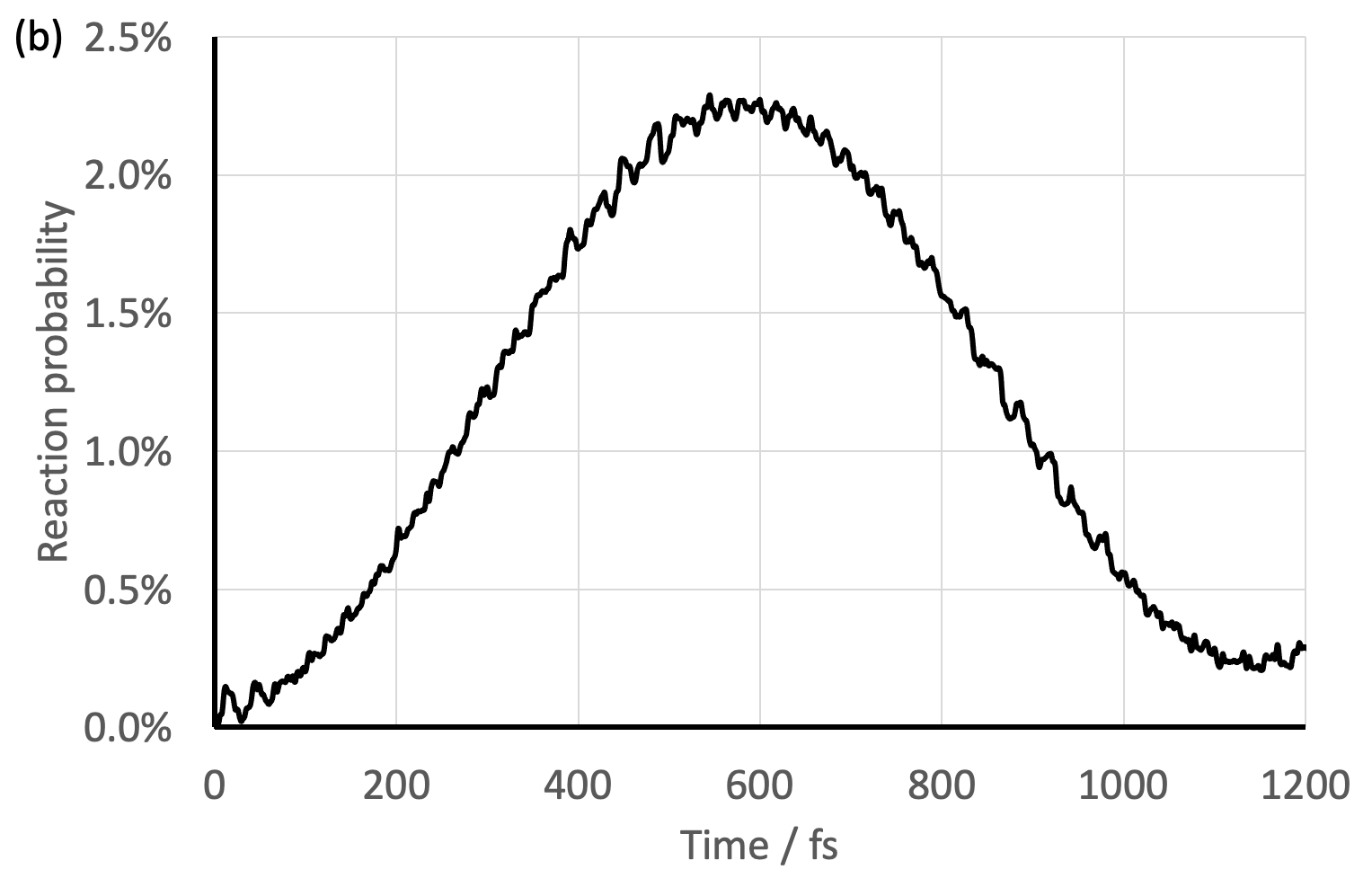
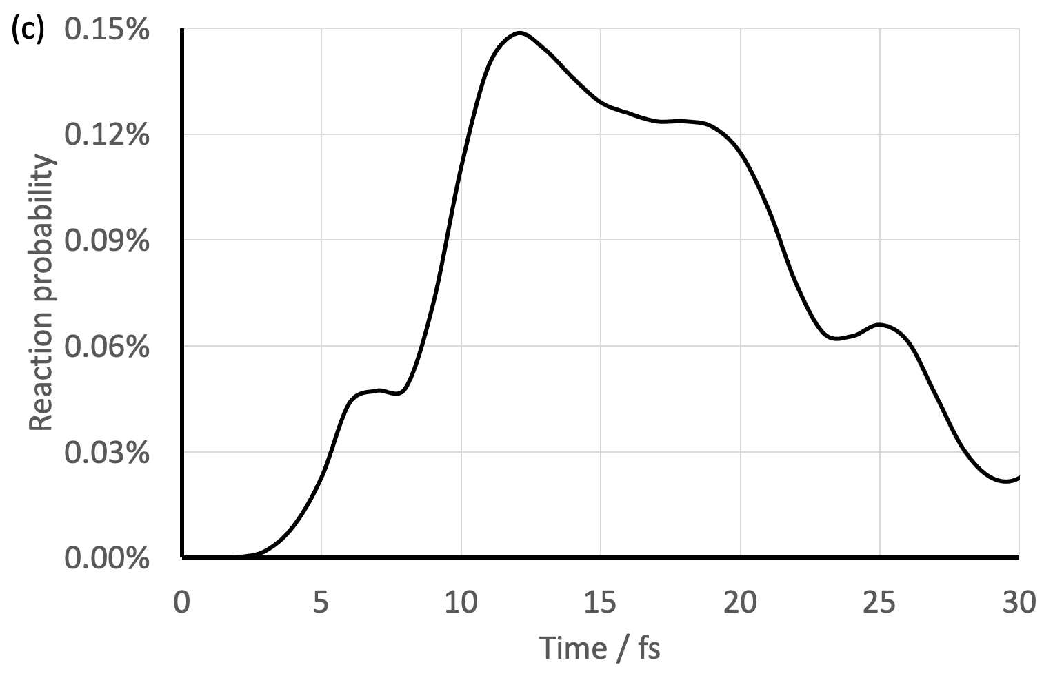
Figure 2. Fully correlated (MCTDH) propagation: Time evolution of the reaction probability, $R(T)$, in the uncoupled model (case 0) ; (a) long times (ground-state tunneling); (b) medium times (excited-state tunneling); (c) short times (quasiharmonic).

All simulations presented below were computed with the Quantics software [24]. Reference simulations denoted as “fully correlated” in the following refer to converged MCTDH calculations where correlated system-bath states are propagated under variational equations of motion [4, 5, 8]. In the specific case of two degrees of freedom, the MCTDH wavefunction ansatz reads as follows, as a generalization of the TDH ansatz,

(10) $$\psi(t,x,y)=\sum_{j_{1}=1}^{n}\sum_{j_{2}=1}^{n}A_{j_{1}j_{2}}(t)\varphi_{j_{1}}(t,x)\chi_{j_{2}}(t,y)$$

The convergence of the multiconfigurational expansion is measured in terms of the so-called natural weights (natural orbital populations) [5]. Typically, expansions up to $n=3$ single-particle functions (orbitals) were necessary in order to achieve convergence for the present systems. We achieved numerically converged situations over long times with natural weights of about 99 %, 1 %, and less than 0.1 % for both degrees of freedom. Further computational details and convergence analysis are provided in the Supplementary Material [LINK]. Related MCTDH calculations for two-dimensional tunneling situations are reported, e.g., in Ref. [17].

5.1. Characteristic times of dynamical simulations

For reference, we first consider the uncoupled model (case $0$; see Table 1). The characteristics of our model are such that we can distinguish three very different time scales, all separated by two orders of magnitude, for the $X$ subsystem dynamics: long, short, and medium times. The long time scale $\sim$100 ps relates to “ground-state tunneling” (induced by the energy splitting between the ground-state tunneling pair); the medium time scale $\sim$ 1 ps is “excited-state tunneling” (first excited tunneling pair splitting); the short time $\sim$ 0.01 ps is due to “quasiharmonic” motion (vibration around the local minimum).

Our preferred observable for monitoring the dynamics will be the “reaction probability”, $R(T)=\langle H_{L}\rangle(T)$. It is defined as the expectation value of the Heaviside step distribution centered at $X=L$, such that it provides a measure of the probability for the system to be in the product region ($X>L$) at any given time.

In the uncoupled case, the time evolution of $R(T)$ shows a perfect tunneling quantum beat between the “reactant” ($X=0$) and “product” ($X=2L$) wells. It oscillates between 0 and 1 with a long period of about 88 ps; see Fig. 2. There is a clear modulation (around 2%) with a medium period of about 1.2 ps. One also notices an extra modulation (around 0.1%) with a short pseudoperiod of about 30 fs and even shorter convoluted temporal structures.

These typical times can be rationalized in terms of the eigenstate decomposition of the initial datum, which corresponds almost perfectly (with 49$\%$) to a one-to-one mixture of the even vs. odd members of the ground-state tunneling pair. As a result, the initial wavepacket is localized on the “reactant” side. The corresponding eigenenergies are 975.92 cm^-1 and 976.30 cm^-1 (wavenumbers will be used as customary energy equivalents within this vibrational context). The tunneling energy splitting of 0.38 cm^-1 corresponds to a ground-state tunneling period of 88.0 ps, as indeed observed and reported above (long time scale). Note that the single-well harmonic approximation of the zero-point energy around the origin is at 1010 cm^-1 (the first tunneling pair is redshifted by about 24 cm^-1 due to the anharmonicity of the double well). The initial wavepacket also contains to some extent a contribution of the next tunneling pair with respect to $X$: i.e., a 1$\%$ component of both members of the excited-state tunneling pair, at 2728 cm^-1 and 2757 cm^-1, split by 29 cm^-1. This induces a medium time scale pertaining to the excited tunneling period of 1.2 ps, as indeed observed. The shorter times are more subtle to interpret. The harmonic approximation around the origin (with an energy quantum of 2000 cm^-1) would induce a harmonic period of 17 fs. The actual difference between the average eigenergies of the first two tunneling pairs is a bit lower, at 1767 cm^-1 with a time of 19 fs, on the same order of magnitude as what we identified as a short pseudoperiod of 30 fs, which can be termed a “quasiharmonic” time. The overall dynamics thus appears to be governed by a four-level eigensystem organized as a “pair of pairs”. Note that the harmonic period for $Y$ is 1.7 ps (with an energy quantum of 20 cm^-1), hence, slightly larger than the medium timescale.

Apart from the details of the interpretation, the present setting is ideal for our study, as we are dealing with three typical timescales that are well separated from each other by about two orders of magnitude.

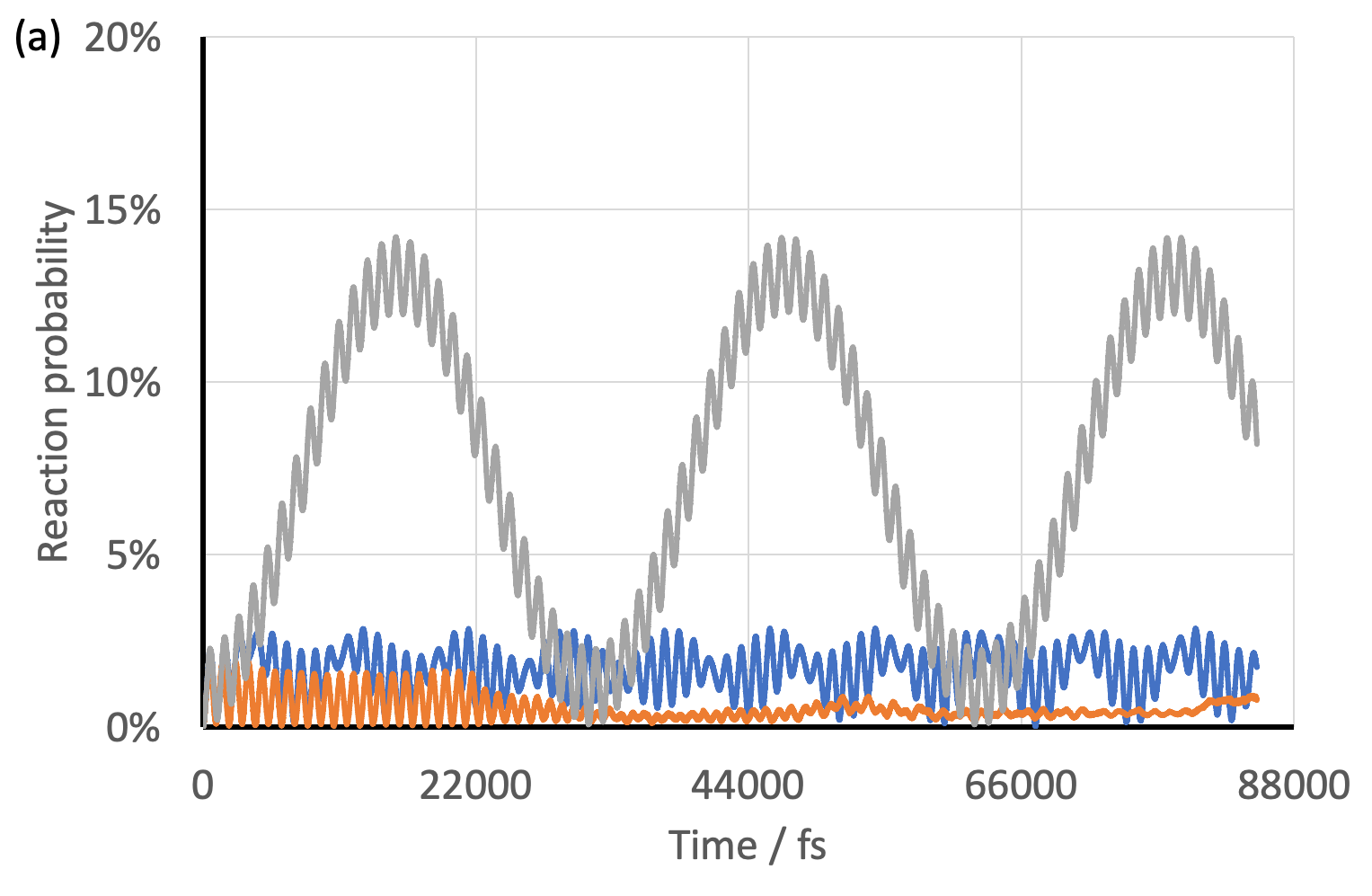
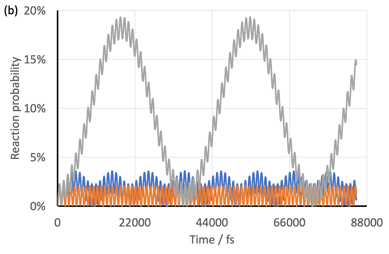
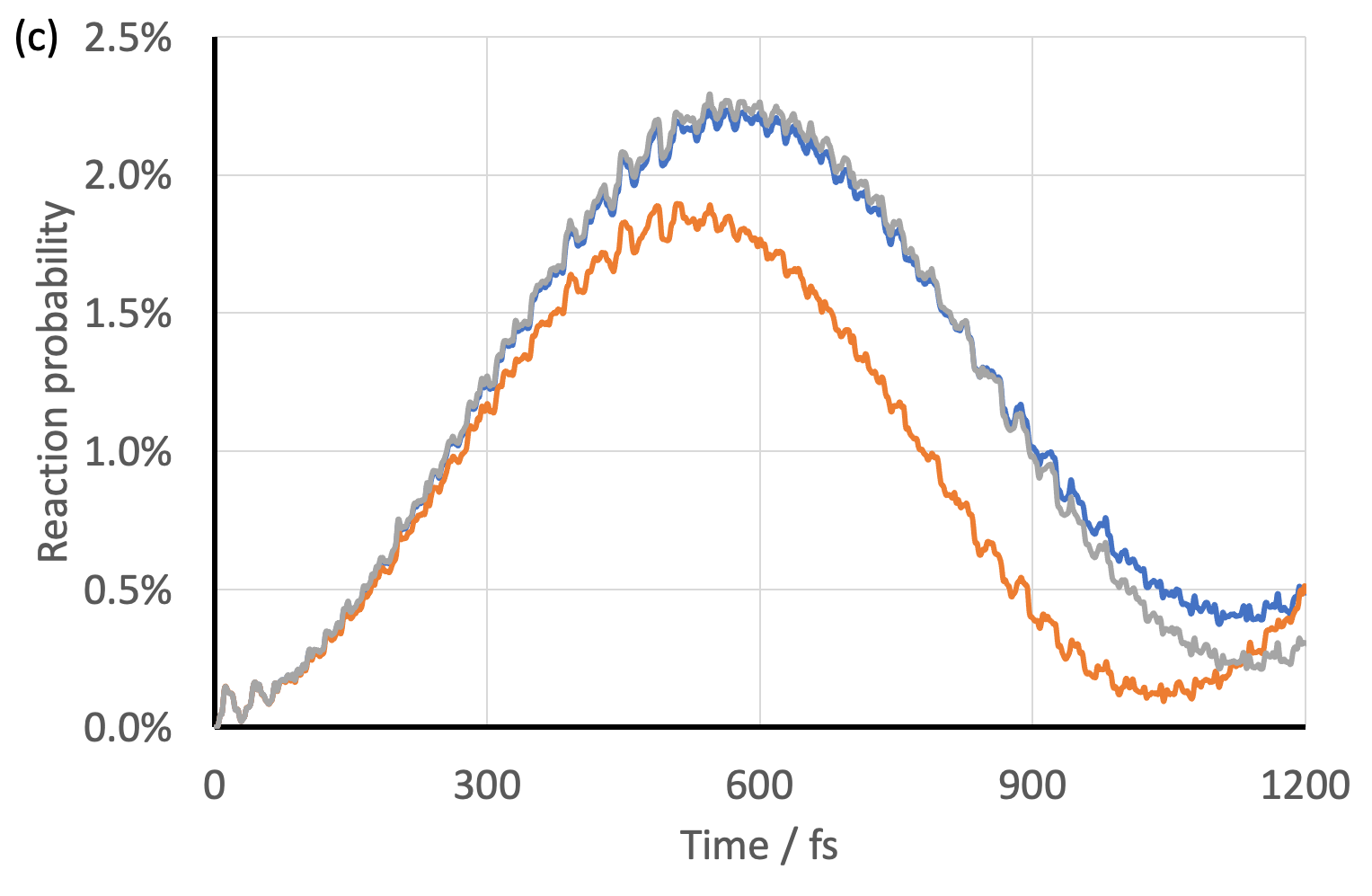
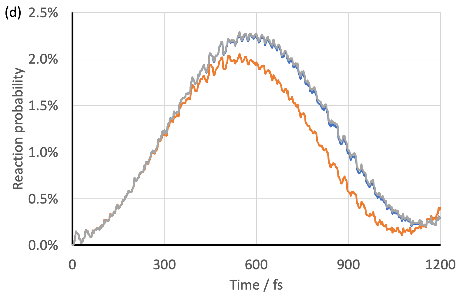
Figure 3. Fully correlated (MCTDH) vs. TDH propagation: Time evolution of the reaction probability, $R(T)$, in three coupled cases (blue: case *; orange: case 3; grey: case 4 – see Table 1); the two left panels show fully correlated (MCTDH), the two right panels TDH propagation; (a, b) long times (ground-state tunneling); (c, d) medium times (excited-state tunneling).

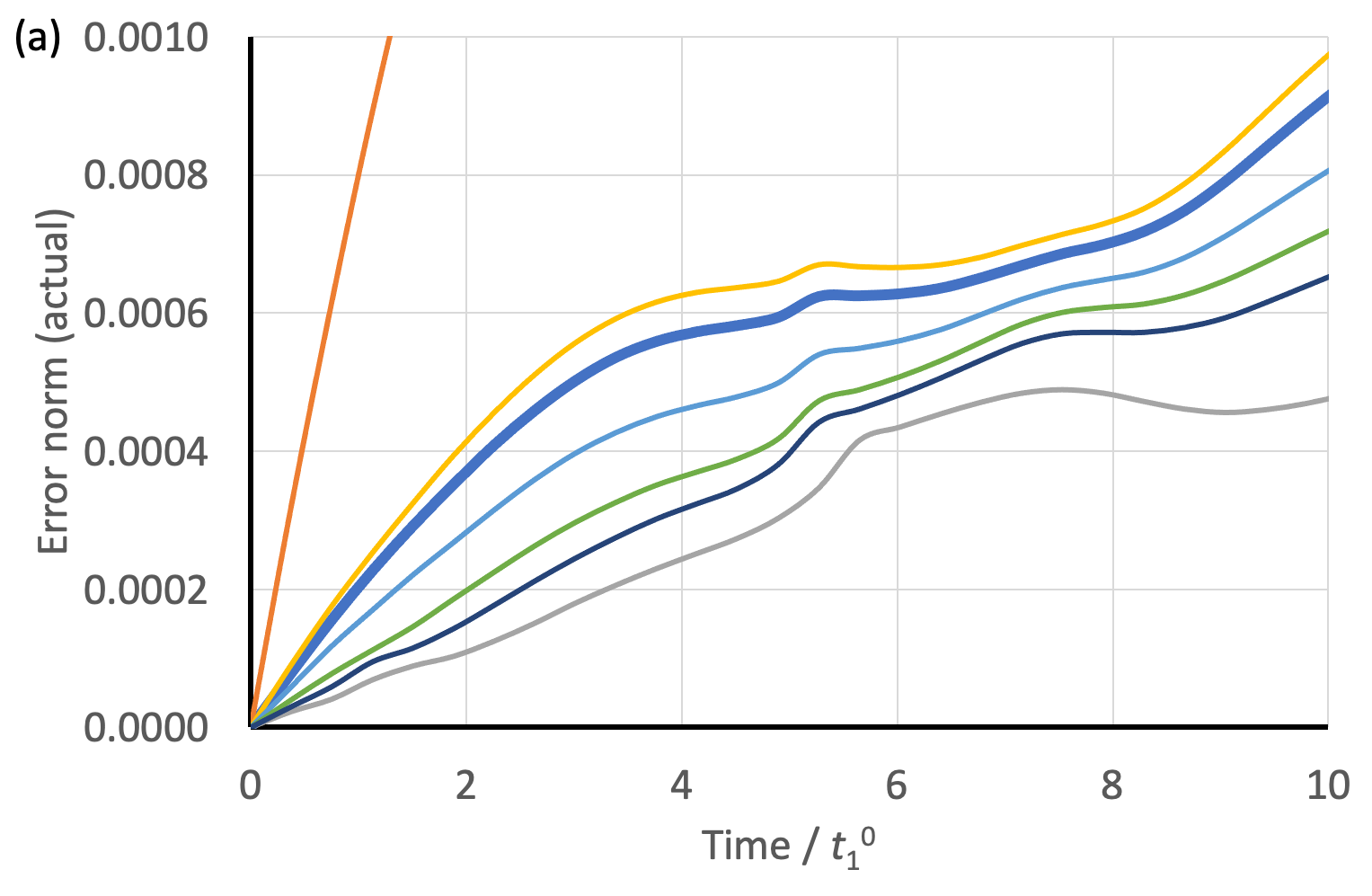
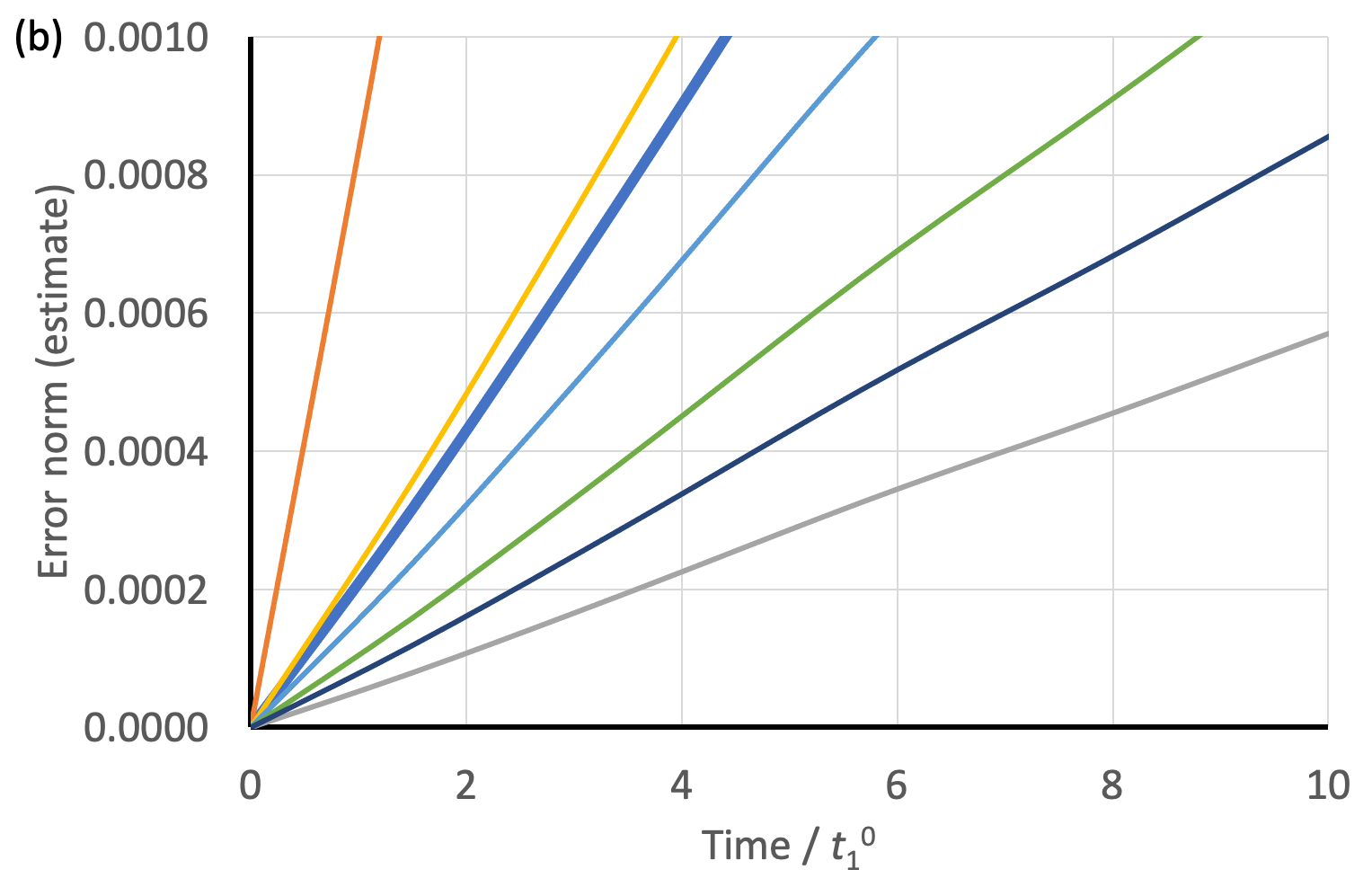
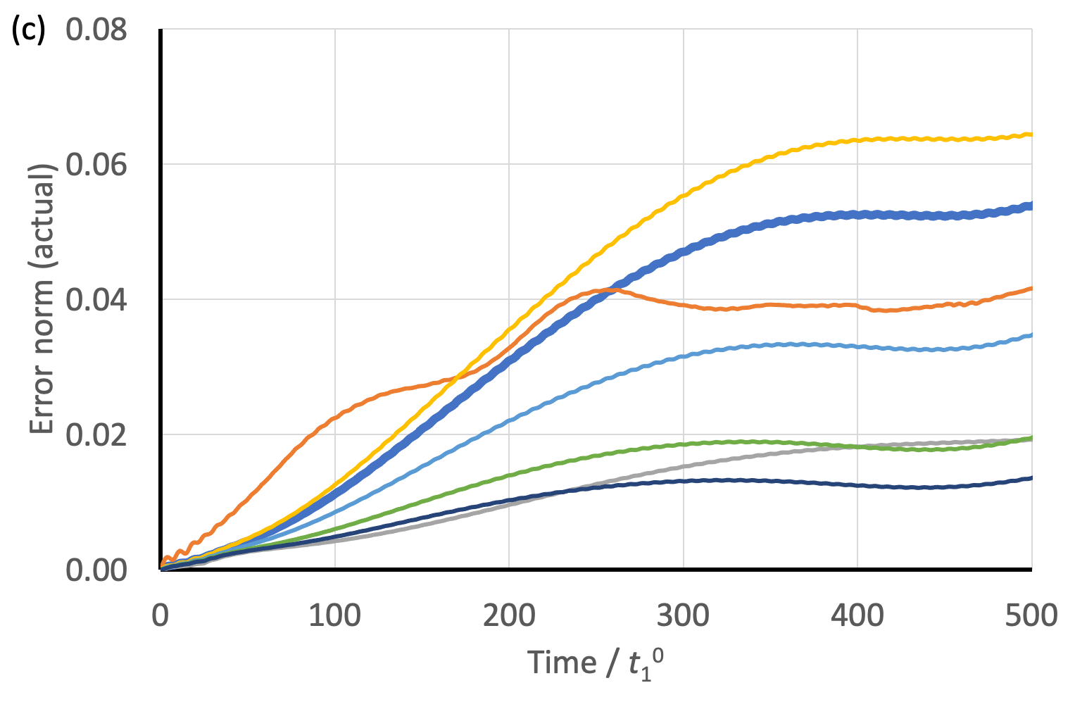
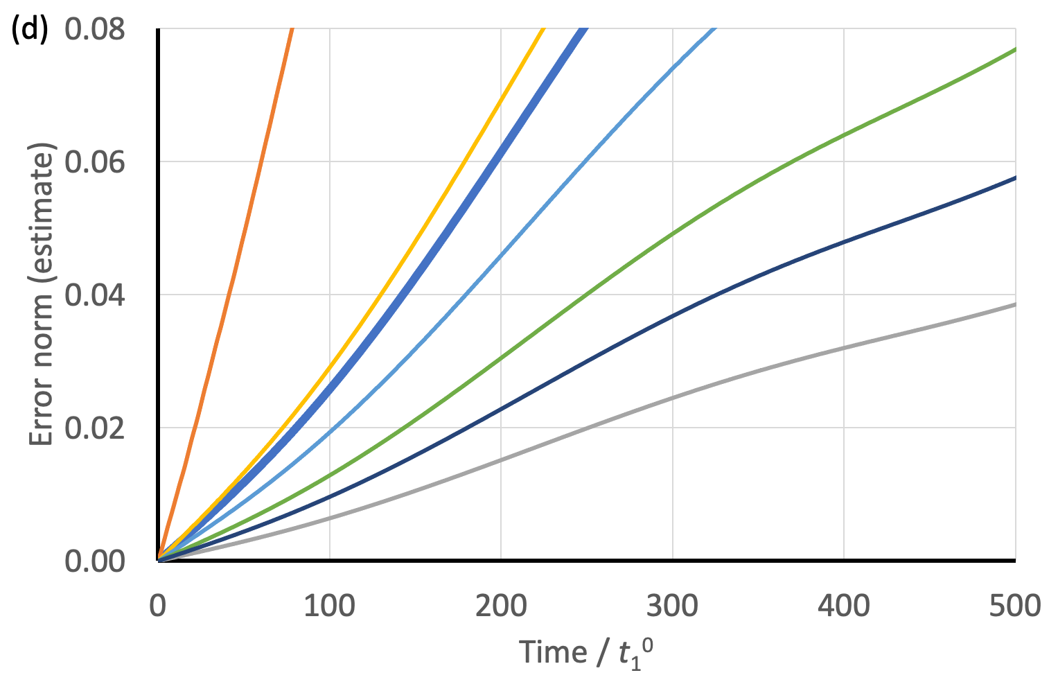
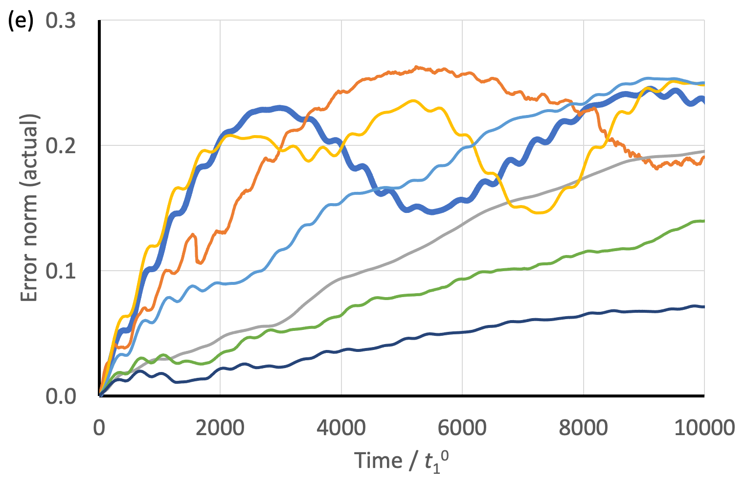
Figure 4. Time evolution of the norm $\|\Psi(T)-U(T)\|_{L^{2}}$ of the actual error and of the error estimate – see Eq. (8) – in seven coupled cases (thick blue: case *; orange: case 3; grey: case 4; yellow: case 5; light blue: case 6; green: case 7; dark blue: case 8 – see Table 1); the three left panels show the actual error, the three right ones the estimate; (a, b) short times; (c, d) medium times; (e, f) long times.

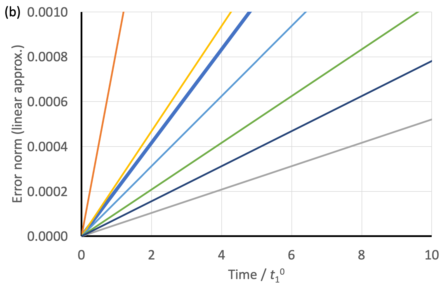
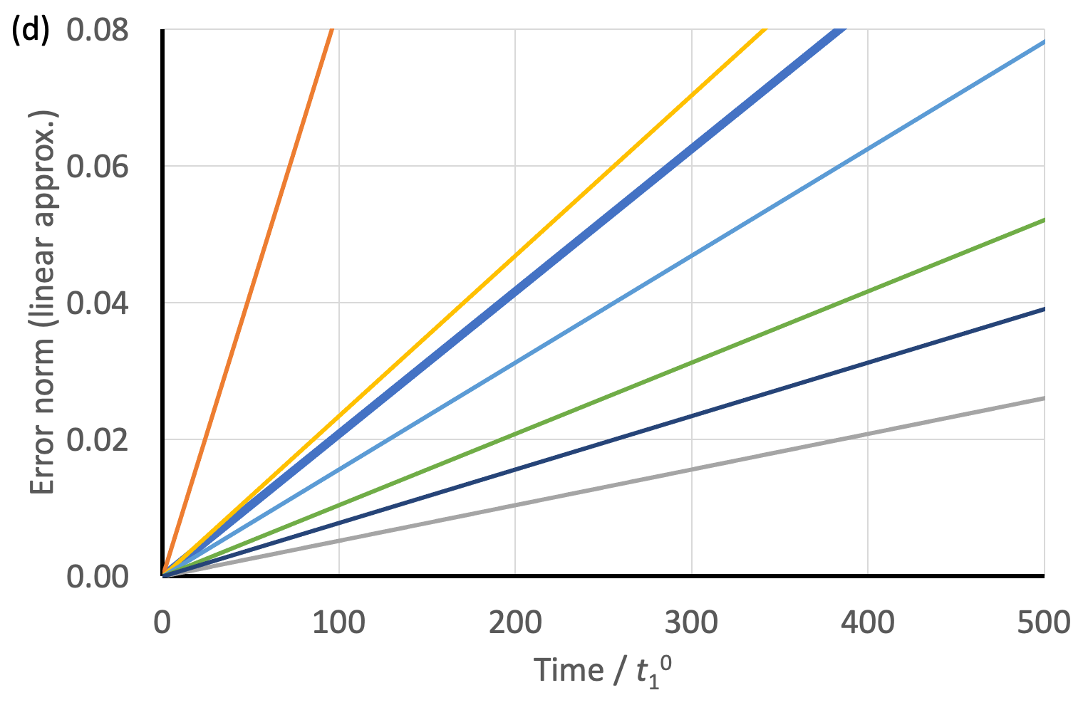
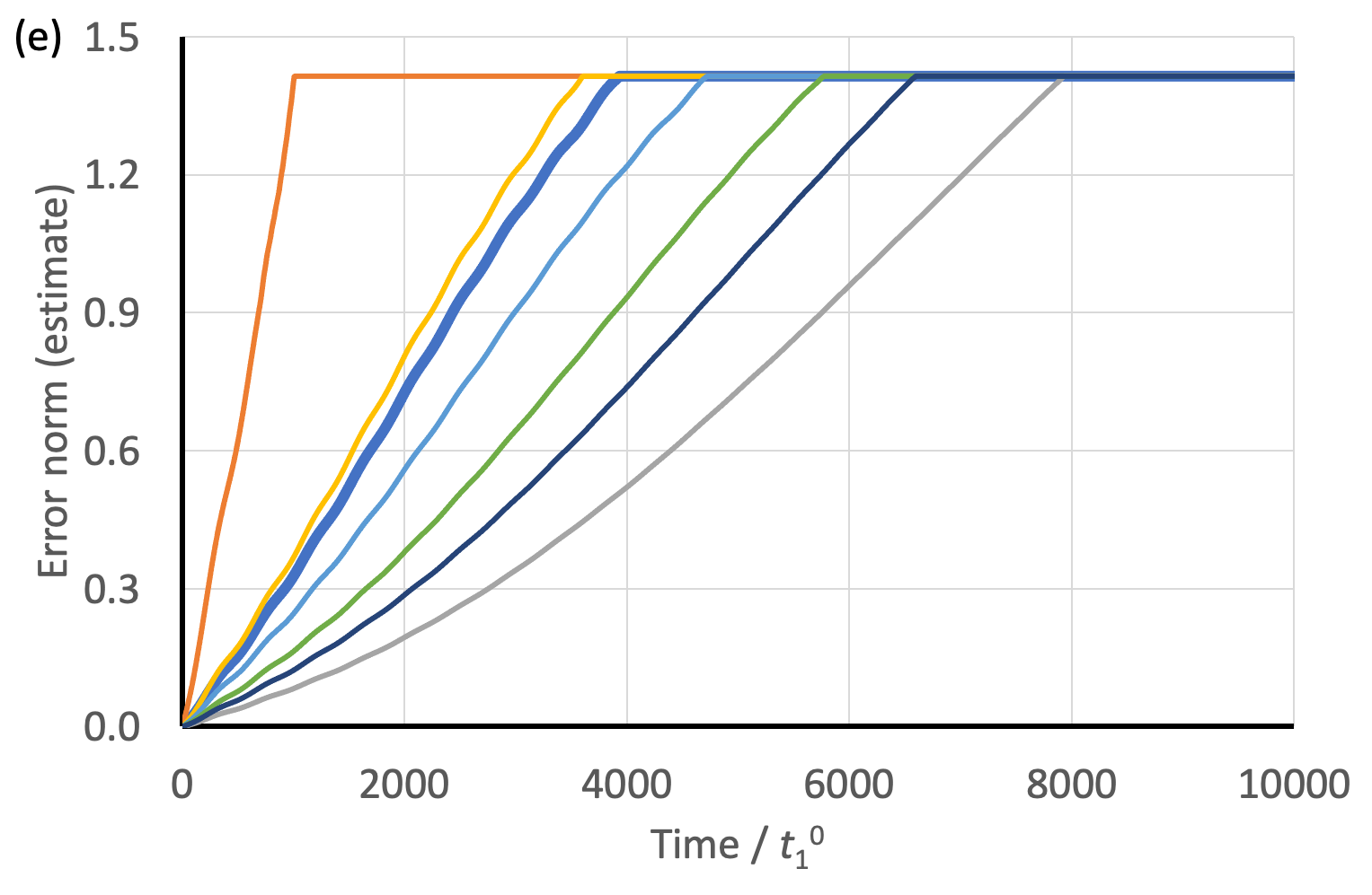
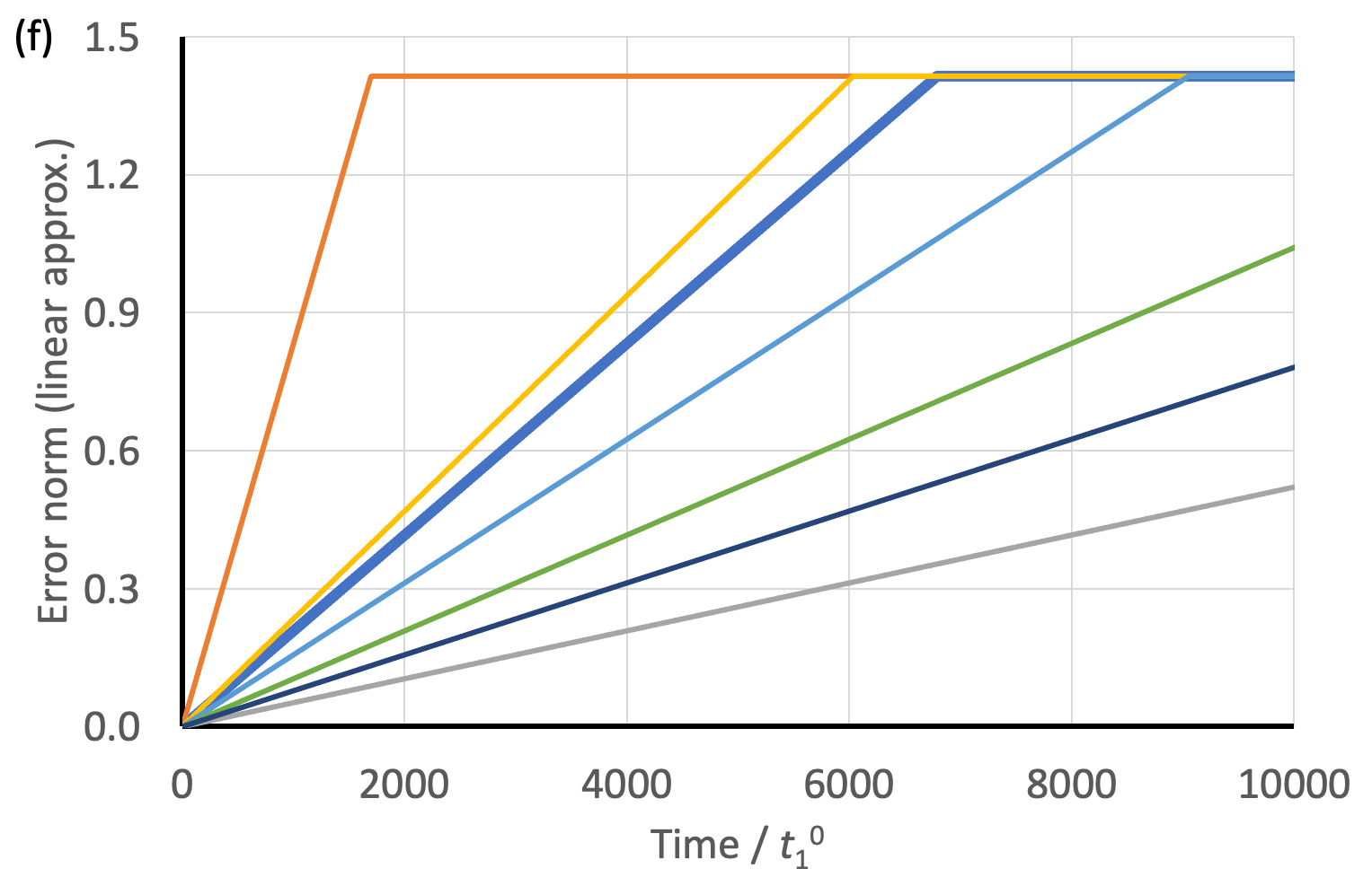
Figure 5. Time evolution of the error estimate – see Eq. (8) – and the linear approximation – see Eq. (9) – in seven coupled cases (thick blue: case *; orange: case 3; grey: case 4; yellow: case 5; light blue: case 6; green: case 7; dark blue: case 8 – see Table 1); the three left panels show the error estimate, the three right ones the linearization; (a, b) short times; (c, d) medium times; (e, f) long times.

We calculated the reaction probability for all cases given in Table 1. Results for the reference model ($*$) and cases 3 and 4 are presented in Fig. 3, for long and medium times both with the fully correlated (MCTDH) and TDH methods. Short-time results are not shown, since these are all virtually identical to the uncoupled case (the dynamics is still uncorrelated).

Upon comparing the left and right panels in Fig. 3, we observe significant differences between fully correlated (MCTDH) and TDH results at long times: (i) the reaction probabilities obtained with TDH do not experience any oscillation damping as opposed to the fully correlated calculations; (ii) the TDH population transfer is slower (smaller rate); (iii) the net transfer is bigger (larger yield).

From a local comparison in time, the error could be considered as very large. However, from a global perspective, the dynamical behavior is qualitatively similar and the orders of magnitude are correct. For example, taking case 4 (grey curves), the tunneling period is 31 ps (fully correlated) vs. 37 ps (TDH) and the rate is 14% (fully correlated) vs. 19% (TDH). Let us now turn to a more detailed analysis of the error in the time-dependent wavefunction.

5.2. Numerical assessment of error estimates

We calculated the actual norm of the error between fully correlated (MCTDH) and TDH wavepackets at all times, $\|\Psi(T)-U(T)\|_{L^{2}}$, in the seven coupled cases given in Table 1 (let us remind that cases 1 and 2 are identical to case * up to within homothetic dynamics in $Y$). These are shown in the left panels of Fig. 4. We also calculated the error estimate given in Eq. (8), as well as its linear approximation defined in Eq. (9), see Fig. 5.

The error estimate given in Eq. (8) appears to be almost exact over dimensionless times $\sim$ 100 $t^{0}_{1}$ where $t^{0}_{1}=$ 2.65 fs (natural time for $X$). It is still dominated by a linear growth with time, as illustrated by its strong similarity with its linear approximation (Eq. (9)). The latter stays quite identical to the former up to about 100 $t^{0}_{1}$ (compare both panels (b) in Figs 5). This reflects small variations of the various moments, consistent with using a quasi-coherent state as initial datum.

Both rigorous and approximate error estimates keep cases ordered over time (no crossing between curves) according to the value of the linear prefactor, $\varpi\varsigma$, while the actual error starts to become more complicated, showing various types of oscillations and some rough saturation around 0.2 to 0.3.

Our estimates keep increasing and stop becoming relevant at $\sim$ 1000 $t^{0}_{1}$; they still can be viewed as upper bounds, though. Note that they finally lose any significance when they reach the critical value $\sqrt{2}$, where orthogonality between the approximate and exact solutions sets in.

6. Conclusions and outlook

Following up on the recently presented mathematical framework for error estimation in the context of composite quantum systems [9], we presented here a first application to a non-trivial two-dimensional system where tunneling motion (i.e., a “reactive subsystem”) is coupled to a quasi-harmonic degree of freedom via a cubic coupling. The values of our system Hamiltonian parameters (frequencies, masses, tunneling length and barrier; see Supplementary Material [LINK]) were chosen so as to correspond to realistic molecular situations. As it occurs, they allow for significant quantum effects, in particular an interesting tunneling process that exhibits three distinct characteristic time scales.

For reference, the reliability of a separable time-dependent Hartree ansatz for the time-evolving wavepacket was assessed by comparison with converged multiconfigurational (MCTDH) calculations that can be considered as numerically exact. The relevant space of system parameters was explored with respect to the coupling strength as well as the relative timescales of the subsystem and the bath.

In the parameter regimes we considered, the TDH approximation represents a good zeroth-order approximation which requires corrections such as to account for correlations. In line with this, tunneling rates and yields differ by no more than a factor of two from the exact result. Yet, the quantitative error is non-negligible, such that the error estimates developed in Ref. [9] are relevant. In the present study, this error is numerically computed and compared with our rigorous mathematical estimates [9]. These estimates were shown to provide a good approximation to the numerically exact error, and yield an almost exact result in the early regime of near-linear growth of the error with time before saturation.

Against the background of a detailed scaling analysis, we further introduced a linearization approach by which an expression for the short-time error estimate was derived, which is found to depend on the frequency ratio of the subsystems. This emphasizes that from the vantage point of the TDH approximation, the frequency ratio rather than the mass ratio of the subsystems is of crucial importance. Again, the linearization estimate was found to provide a valid approximation, even beyond the shortest time scale.

The present work paves the way for extensions of error analysis to other types of wavefunction ansatz, such as multiconfigurational forms of MCTDH type [5, 25], and especially Gaussian-based hybrid wavefunctions such as employed in the G-MCTDH method [26, 27]. The model that we used showed moderate failures of TDH that have observable consequences on, for example, the reaction probability. It could thus be useful for benchmarking a hierarchy of methods of various sophistication.

Finally, as mentioned in Sec. 2, the present treatment can be generalized to a genuine system-bath situation where the subsystems are subject to external fluctuations inducing dissipation [28, 29]. In this context, the present perspective immediately connects to a non-Markovian treatment of structured environments which can be decomposed in terms of effective environmental modes [15, 16]. From this viewpoint, the system-bath boundary can be shifted such as to include a set of environmental modes as additional subsystems in an explicit treatment, while a residual bath is included by a Markovian approximation. This type of approach has been recently employed in the context of two-dimensional molecular tunneling dynamics [17], in a similar parameter range as specified in the present model. These models permit to further investigate fluctuation-induced enhancement or reduction of tunneling, localization effects, and decoherence, which are ubiquitous effects far beyond the molecular tunneling situation considered here. Including fluctuations and dissipation is obviously of general importance in quantum metastable systems [10, 11, 30]. This direction provides a natural extension to the treatment employed in the present work.

References

- [1] P. A. M. Dirac. Note on exchange phenomena in the thomas atom. Mathematical Proceedings of the Cambridge Philosophical Society, 26(3), 1930.
- [2] R. B. Gerber, V. Buch, and M. A. Ratner. Time-dependent self-consistent field approximation for intramolecular energy transfer: I. Formulation and application to dissociation of van der Waals molecules. J. Chem. Phys., 77:3022, 1982.
- [3] R. B. Gerber and M. A. Ratner. Mean-field models for molecular states and dynamics: new developments. J. Phys. Chem., 92(11):3252–3260, 1988.
- [4] H.-D. Meyer, U. Manthe, and L. S. Cederbaum. The multi-configurational time-dependent Hartree approach. Chem. Phys. Lett., 165(1):73–78, 1990.
- [5] M.H. Beck, A. Jäckle, G.A. Worth, and H.-D. Meyer. The multiconfiguration time-dependent Hartree (MCTDH) method: a highly efficient algorithm for propagating wavepackets. Physics Reports, 324(1):1–105, 2000.
- [6] F. Schroeder and A. W Chin. Simulating open quantum dynamics with time-dependent variational matrix product states: towards microscopic correlation of environment dynamics and reduced system evolution. Phys. Rev. B, 93:075105, 2016.
- [7] A. Strathearn, P. Kirton, D. Kilda, J. Keeling, and B. W. Lovett. Efficient non-Markovian quantum dynamics using time-evolving matrix product operators. Nature Communications, 9:3322, 2018.
- [8] C. Lubich. From quantum to classical molecular dynamics: reduced models and numerical analysis. European Mathematical Society (EMS), Zürich, 2008.
- [9] I. Burghardt, R. Carles, C. Fermanian Kammerer, B. Lasorne, and C. Lasser. Separation of scales: dynamical approximations for composite quantum systems. J. Phys. A, 54(41):Paper No. 414002, 36, 2021.
- [10] U. Weiss. Quantum dissipative systems, 4th Ed. World Scientific, Singapore, 2012.
- [11] H.-P. Breuer and F. Petruccione. The theory of open quantum systems. Oxford University Press, Oxford, 2002.
- [12] A. M. Levine, M. Shapiro, and E. Pollak. Hamiltonian theory for vibrational dephasing rates of small molecules in liquids. J. Chem. Phys., 88:1959, 1988.
- [13] M. Gruebele. Quantum dynamics and control of vibrational dephasing. J. Phys.: Condens. Matter, 16:R1057, 2004.
- [14] P. R. Bunker and P. Jensen. Molecular symmetry and spectroscopy. NRC Research Press, Ottawa, 2006.
- [15] R. Martinazzo, K. H. Hughes, and I. Burghardt. Unraveling a Brownian particle’s memory with effective mode chains. Phys. Rev. E, 84:030102, 2011.
- [16] R. Martinazzo, B. Vacchini, K. H. Hughes, and I. Burghardt. Communication: Universal Markovian reduction of Brownian particle dynamics. J. Chem. Phys., 134:011101, 2011.
- [17] D. Picconi and I. Burghardt. Open system dynamics using Gaussian-based multiconfigurational time-dependent Hartree wavefunctions: Application to environment-modulated tunneling. J. Chem. Phys., 150:224106, 2019.
- [18] H. Nakamura and G. Milnikov. Quantum Mechanical Tunneling in Chemical Physics. CRC Press, 1st edition, 2013.
- [19] N. Shida, P. F. Barbara, and J. E. Almlöf. A theoretical study of multidimensional nuclear tunneling in malonaldehyde. J. Chem. Phys., 91:4061, 1989.
- [20] T. N. Wassermann, D. Luckhaus, S. Coussan, and M. A. Suhm. Proton tunneling estimates for malonaldehyde vibrations from supersonic jet and matrix quenching experiments. Phys. Chem. Chem. Phys., 8(20):2344, 2006.
- [21] K. C. Woo and S. K. Kim. Multidimensional H Atom Tunneling Dynamics of Phenol: Interplay between Vibrations and Tunneling. J. Phys. Chem. A, 123(8):1529–1537, 2019.
- [22] C. Qu, P. L. Houston, R. Conte, A. Nandi, and J. M. Bowman. MULTIMODE Calculations of Vibrational Spectroscopy and 1d Interconformer Tunneling Dynamics in Glycine Using a Full-Dimensional Potential Energy Surface. J. Phys. Chem. A, 125(24):5346–5354, 2021.
- [23] B. Lasorne, G. Dive, D. Lauvergnat, and M. Desouter-Lecomte. Wave packet dynamics along bifurcating reaction paths. J. Chem. Phys., 118(13):5831–5840, 2003.
- [24] G. A. Worth, K. Giri, G. W. Richings, I. Burghardt, M. H. Beck, A. Jäckle, and H.-D. Meyer. Quantics package, version 2.0, 2020.
- [25] F. Gatti, B. Lasorne, H.-D. Meyer, and A. Nauts. Applications of Quantum Dynamics in Chemistry. Lectures Notes in Chemistry. Springer International Publishing, 2017.
- [26] I. Burghardt, H.-D. Meyer, and L. S. Cederbaum. Approaches to the approximate treatment of complex molecular systems by the multiconfiguration time-dependent Hartree method. J. Chem. Phys., 111:2927, 1999.
- [27] S. Römer and I. Burghardt. Towards a variational formulation of mixed quantum-classical molecular dynamics. Molecular Physics, 111(22-23):3618–3624, 2013.
- [28] A. O. Caldeira and A. J. Leggett. Influence of Dissipation on Quantum Tunneling in Macroscopic Systems. Phys. Rev. Lett., 46(4):211, 1981.
- [29] A. J. Leggett, S. Chakravarty, A. T. Dorsey, Matthew P. A. Fisher, Anupam Garg, and W. Zwerger. Dynamics of the dissipative two-state system. Rev. Mod. Phys., 59:1–85, 1987.
- [30] B. Spagnolo, A. Carollo, and D. Valenti. Enhancing metastability by dissipation and driving in an asymmetric bistable quantum system. Entropy, 20(4):226, 2018.