DenseGAP: Graph-Structured Dense Correspondence Learning with Anchor Points

Abstract

Establishing dense correspondence between two images is a fundamental computer vision problem, which is typically tackled by matching local feature descriptors. However, without global awareness, such local features are often insufficient for disambiguating similar regions. And computing the pairwise feature correlation across images is both computation-expensive and memory-intensive. To make the local features aware of the global context and improve their matching accuracy, we introduce DenseGAP, a new solution for efficient Dense correspondence learning with a Graph-structured neural network conditioned on Anchor Points. Specifically, we first propose a graph structure that utilizes anchor points to provide sparse but reliable prior on inter- and intra-image context and propagates them to all image points via directed edges. We also design a graph-structured network to broadcast multi-level contexts via light-weighted message-passing layers and generate high-resolution feature maps at low memory cost. Finally, based on the predicted feature maps, we introduce a coarse-to-fine framework for accurate correspondence prediction using cycle consistency. Our feature descriptors capture both local and global information, thus enabling a continuous feature field for querying arbitrary points at high resolution. Through comprehensive ablative experiments and evaluations on large-scale indoor and outdoor datasets, we demonstrate that our method advances the state-of-the-art of correspondence learning on most benchmarks.

I Introduction

Image correspondence is the foundation of many computer vision tasks, such as geometric matching [1, 2, 3], pose estimation [4, 5], visual localization [6], and optical flow [1, 2, 3, 7]. Although being long explored, it remains an open question, especially for images under large appearance or view changes, or containing textureless or repetitive regions. The classic solution is based on keypoint detection and matching [8, 9, 5]. This line of methods is highly efficient but limited by the missing-detection issue [10]. Thus, the more recent works eliminate the dependency on keypoint detection by considering every point for building dense correspondence.

Recent works on dense correspondence learning build 4D correlations between images using local features extracted for each point, followed by a neighbor consensus filtering strategy to select confident matches [11, 10, 12, 13]. These methods are effective in finding denser matches but still suffer from two major limitations: (1) computing full points correlation is expensive and memory-intensive, especially on high-resolution images; (2) the extracted local features lack global context, making them indistinguishable in textureless or repetitive regions. The follow-up methods [12, 14] adopt coarse-to-fine frameworks to reduce the computational cost but struggle with the small receptive fields. To overcome them, we propose to utilize sparse correspondences as a bridge to connect every point in the global context, inspired by that humans typically use global information constructed by a few salient points to distinguish similar regions in a scene.

In this paper, we present a novel way of introducing sparse priors to dense correspondence learning using anchor points, a set of paired salient points corresponded across images. With these anchor points, we propose to learn a context-aware feature field for querying correspondence at arbitrary image positions. We adopt a graph representation that connects the anchor points to every image position so as to model different levels of context and propagate them to the whole graph. Based on this representation, to integrate the global information into the local features, we further design three simple but effective message-passing layers: the inter-points layer binds anchor points to introduce the inter-image correlation, the intra-points layer aggregates information among anchor points within an image and builds the intra-image context, and the point-to-image layer broadcasts the above global contexts to every point and fuses it with the local features. Utilizing the predicted features, we finally present a coarse-to-fine framework to learn accurate dense correspondence based on cycle consistency. Extensive ablative experiments and comparisons show that our learned feature descriptors effectively boost the performance of dense correspondence prediction. In particular, our approach can help in complex tasks such as surface normal prediction, depth estimation, and object detection, where global context plays a critical role in extracting point-level information.

Our main contributions are summarised as follows: Firstly, we propose to use anchor points as priors for dense correspondence learning in a graph structure, which connects all local points in a global context. Secondly, we design a network based on the graph representation with three light-weighted message-passing layers for propagating and aggregating multi-level context information. Finally, our novel dense correspondence prediction pipeline achieves state-of-the-art (SOTA) performance, which supports arbitrary correspondence query for high-resolution input images and effectively embeds the global context to the local feature descriptors.

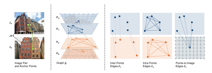
Figure 1: Illustration of the concept. From left to right: (1) Showcase of how anchor points guide our model to find dense correspondences; (2) Visualization of our designed graph; (3) Three types of edges in our graph.

II Related Work

Image Correspondence

The well-adopted pipeline for establishing image correspondence usually consists of feature detection [8, 15, 16, 17, 18], description [19, 20, 21, 22, 23, 24, 25, 26, 27, 28], and matching [5]. The typical drawback of these detector-based methods is the missing-detection problem, which limits the accuracy and the number of matches. To address this problem, detector-free approaches are explored. Some achieve feature matching by extracting features on a dense grid across the images [11] and use coarse-to-fine frameworks to reduce memory footprint and improve fine-level matching  [10, 12, 6]. However, these frameworks require heavy computation of inter-image correlation and neglect the contextual cues. Another line of the detection-free methods [1, 2, 3, 29] aims to generate pixel-level correspondence and bridge correspondence learning and optical flow estimation. They work well for continuous frames but are inadequate to handle image pairs with large displacements. Recently, the concurrent works [4, 7] involve global context between matches by using transformers [30] which achieve great success in many NLP and vision tasks [31, 32, 33] using the attention mechanism. Different from them, we propose to adopt sparse correspondence as prior and design light-weighted network layers to efficiently propagate the contextual information to all image points, allowing predicting dense correspondence for arbitrary points.

Graph-Structured Network

The graph-structured representation is applied in various domains, such as image [34, 35], video [36], skeleton [37, 38] and mesh [39, 40] thanks to the flexibility of this data structure. Meanwhile, more interests has put into relating graph representation with neural networks. The framework of graph neural network (GNN) is first proposed in [41], which formulates as node, edges, message-passing layers to assemble information from a graph structure. Inspired by GNN, some methods apply graph networks to vision tasks such as image recognition [42], object detection [43], point cloud learning [44] and so on. Our work introduces anchor points to bring the graph representation into correspondence learning. The graph representation is inspired by SuperGlue [5] which proposes a graph neural network for matching sparse keypoints between images. Different from SuperGlue [5], we propose a more sophisticated graph to model multi-level contexts using sparse correspondence as prior and develop a general architecture to infuse the contextual information into local features. We follow the attention-based mechanism of Transformer [30] to implement message-passing layers in the graph network, while Transformer [30] is also used by recent works [4, 7] in a different way.

III Method

III-A Anchor Points

We propose to solve the problem of finding dense correspondence between a pair of images by first extracting a feature descriptor for arbitrary query points in one image and then using it to compute the correspondence in the other image. To efficiently encode the global information (e.g. inter- and intra-image context) in the feature descriptor, we introduce anchor points to bridge all the points across images. The anchor points are a set of corresponding points from a pair of images that usually specify spatial locations of the salient features (e.g. blobs, corners). They can be obtained by off-the-shelf sparse matching algorithms (e.g. [5, 24]), serving as reliable priors and modeling global contexts. Then we build a graph with anchor points and image points as nodes, connecting them with directed edges. By applying the message-passing mechanism [45], we achieve the information propagation in the graph and aggregation for each node.

Given a pair of images $(I_{a},I_{b})$, and a normalized pixel coordinate $x\in[0,1]^{2}$ in $I_{a}$ as the query point, our target is to find its correspondence $y\in[0,1]^{2}$ in $I_{b}$. To achieve it, we adopt the approach introduced in [14] by extracting feature descriptors $F_{a}$ and $F_{b}$ of both images and computing $y$ as the expectation of the correlation-based distribution over $I_{b}$:

$$y=\sum_{y\in I_{b}}y\cdot\text{Softmax}_{y}(F_{a}(x)^{T}F_{b}(y)).$$ (1)

Note that $x\in[0,1]^{2}$ means a continuous coordinate and $x\in I_{a}$ indicates the pixel of $I_{a}$. To learn $F_{a}$ and $F_{b}$, we use anchor points, $\mathcal{A}_{a}\subset[0,1]^{2}$, $\mathcal{A}_{b}\subset[0,1]^{2}$ and their one-to-one correspondence ${\mathcal{A}}=\{(x,y)|x\in\mathcal{A}_{a},y\in\mathcal{A}_{b}\}$ as prior. We connect them with the image points in a directed graph ${\mathcal{G}}$, as shown in Fig. 1. In ${\mathcal{G}}$, we first build nodes for ${\mathcal{A}}$, i.e., ${\mathcal{V}}_{x}=\{v_{x}|x\in{\mathcal{A}_{a}}\}$ and ${\mathcal{V}}_{y}=\{v_{y}|y\in{\mathcal{A}_{b}}\}$, and nodes for all image points of $I_{a}$ and $I_{b}$, i.e., ${\mathcal{V}}_{a}=\{v_{x}|x\in I_{a}\}$ and ${\mathcal{V}}_{b}=\{v_{y}|y\in I_{b}\}$. Then we connect them by three types of directed edges which we denote as $(v_{s},v_{r})$:

$$\begin{split}{\mathcal{E}}_{c}&=\{(v_{s},v_{r})|(s,r)\in{\mathcal{A}}\}\cup\{(v_{r},v_{s})|(s,r)\in{\mathcal{A}}\},\\ {\mathcal{E}}_{s}&=\{(v_{s},v_{r})|v_{s},v_{r}\in{\mathcal{V}}_{x}\}\cup\{(v_{s},v_{r})|v_{s},v_{r}\in{\mathcal{V}}_{y}\},\\ {\mathcal{E}}_{i}&=\{(v_{s},v_{r})|v_{s}\in{\mathcal{V}}_{x},v_{r}\in{\mathcal{V}}_{a}\}\cup\\ &\quad\{(v_{s},v_{r})|v_{s}\in{\mathcal{V}}_{y},v_{r}\in{\mathcal{V}}_{b}\}.\end{split}$$ (2)

${\mathcal{E}}_{c}$ indicate inter-points edges between anchor points from both images for inter-image communication; ${\mathcal{E}}_{s}$ represent intra-points edges between anchor points within the same image for intra-image communication; ${\mathcal{E}}_{i}$ are points-to-image edges from anchor points to image points, used to broadcast the information from anchor points to everywhere. Thus, the graph is represented as ${\mathcal{G}}=\left({\mathcal{V}}=\{{\mathcal{V}}_{a},{\mathcal{V}}_{b},{\mathcal{V}}_{x},{\mathcal{V}}_{y}\},{\mathcal{E}}=\{{\mathcal{E}}_{c},{\mathcal{E}}_{s},{\mathcal{E}}_{i}\}\right)$.

We build a neural network based on this graph structure. Inspired by message-passing concept in graphical models, we design a message-passing layer for each type of edges ${\mathcal{E}}^{\prime}\in{\mathcal{E}}$:

$$\begin{split}z^{a}_{r}&=\sum_{(v_{s},v_{r})\in\mathcal{E^{\prime}}}\alpha_{\mathcal{E}^{\prime}}(z^{in}_{s})\cdot\beta_{\mathcal{E}^{\prime}}(z^{in}_{s},z^{in}_{r}),\\ z^{out}_{r}&=\rho_{\mathcal{E}^{\prime}}(z^{in}_{r},z^{a}_{r}).\end{split}$$ (3)

In detail, the message-passing layer first reprojects the input node attributes $z_{s}^{in}$ by $\alpha_{\mathcal{E}^{\prime}}$, and then calculates the messages passed through the edges $(v_{s},v_{r})$ by $\beta_{\mathcal{E}^{\prime}}$. Finally, it aggregates all information sent to the target node $v_{r}$ (denoted as $z_{r}^{a}$) and outputs the updated attributes by a feed-forward function ${\rho_{\mathcal{E}^{\prime}}}$. All the functions in Eq. 3 vary according to the edge types.

III-B Message-Passing Layers

Inter-Points Message-Passing Layer

This layer updates the features of anchor points using their counterparts in the other image through the edges ${\mathcal{E}}_{c}$. The anchor points are connected in a bipartite subgraph by edges ${\mathcal{E}}_{c}$. In this subgraph, all nodes have indegree and outdegree of $1$ as they are one-to-one paired. For this particular structure, we build a simple but effective layer by assigning the functions in Eq. 3:

$$\begin{split}\alpha_{\mathcal{E}_{c}}(z_{s})&=1,\\ \beta_{\mathcal{E}_{c}}(z_{s},z_{r})&=\mathcal{F}_{corr}(z_{s}\odot z_{r}),\\ \rho_{\mathcal{E}_{c}}(z_{r},z_{a})&=z_{r}+z_{a},\end{split}$$ (4)

where $\odot$ means concatenation. The function first concatenates input features in a specified order (i.e. $s$ first and then $r$), and then applies a two-layer multilayer perceptron (MLP) $\mathcal{F}_{corr}$ to get the aggregated information as the residual. The edges $(x_{s},x_{r})\in\mathcal{E}_{c}$ are existing in pairs, and thus this layer updates the features for anchor points in a symmetric way.

Intra-Points Message-Passing Layer

This layer updates the feature descriptors of anchor points by aggregating messages across the edges ${\mathcal{E}}_{s}$. Each node is connected to all the others by ${\mathcal{E}}_{s}$ within the image, forming a complete subgraph. We update the node attribute based on the multi-head attention (MHA) used in [30], which has been proved a highly effective neural architecture in various mainstream vision tasks [32, 31], including building sparse correspondence [5]. In our setting, each node is updated based on a weighted sum over its neighbours during the aggregation step (Fig. 2). For each node $v_{r}$ connected by a set of incoming edges $(v_{s},v_{r})$, the first step is to generate the query vector $Q^{h}_{r}$ from $z_{r}$, and the key $K^{h}_{s}$ and value vector $V^{h}_{s}$ from $z_{s}$ for each head $h$. As in Eq. 5, in each head, we sum up the value of all $z_{s}$ weighted by the attention $A^{h}_{s,r}$ calculated using the query and key vectors. Finally, we concatenate the aggregated value of all heads and use a feed-forward network $\mathcal{F}_{out}$ to refine the output.

$$\begin{split}Q^{h}_{r}&=\textbf{W}^{h}_{q}z_{r},[K^{h}_{s},V^{h}_{s}]=[\textbf{W}^{h}_{k},\textbf{W}^{h}_{v}]z_{s},\\ A^{h}_{s,r}&=\text{Softmax}_{s}\left((K^{h}_{s})^{T}Q^{h}_{r}/\sqrt{d_{k}}\right),\\ V^{h}_{r}&=\sum_{s}A^{h}_{s,r}\cdot V^{h}_{s},\\ z_{r}^{out}&=\mathcal{F}_{out}(z_{r}+\textbf{W}_{out}(V^{0}_{r}\odot V^{1}_{r}\odot\ldots\odot V^{h}_{r})),\end{split}$$ (5)

where $\textbf{W}_{q},\textbf{W}_{k},\textbf{W}_{v},\textbf{W}_{out}$ are weight matrices, and $d_{k}$ is the dimension of $K^{h}_{s}$.

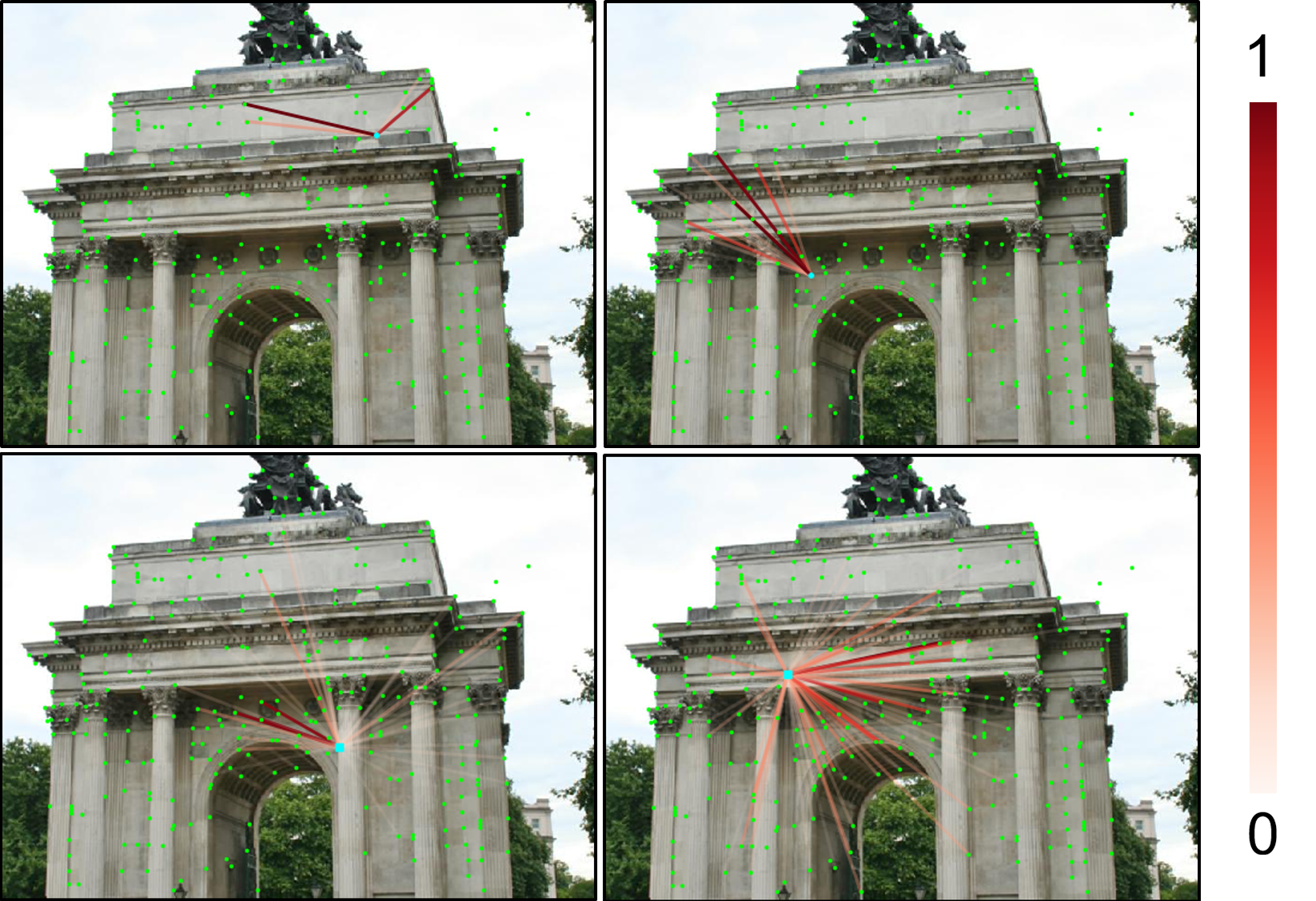
Figure 2: Visualization of attention. Row 1: Attention in intra-points message-passing layer; Row 2: Attention in point-to-image message-passing layer.

We adapt this attention model to our message-passing layer, where the functions in Eq. 3 for this layer are defined as:

$$\begin{split}\alpha^{h}_{\mathcal{E}_{s}}(z_{s})&=V^{h}_{s},\\ \beta^{h}_{\mathcal{E}_{s}}(z_{s},z_{r})&=A^{h}_{s,r},\\ \rho_{\mathcal{E}_{s}}(z_{r},z_{a})&=\mathcal{F}_{out}(z_{r}+\textbf{W}_{out}(z^{0}_{a}\odot z^{1}_{a}\odot\ldots\odot z^{h}_{a})).\\ \end{split}$$ (6)

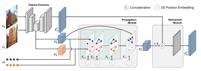
Figure 3: Overview of the framework. Given two images and anchor points, we first extract the coarse and fine feature maps of each image. Then we obtain the features of anchor points from the coarse feature maps as input to the Propagation Module. The output of the module is updated coarse feature maps, and is then fed with the fine feature maps to the Refinement Module. This module finally generates the updated fine feature maps.

Points-to-Image Message-Passing Layer

This layer is designed to propagate the information learned by anchor points to all image points along the edges ${\mathcal{E}_{i}}$. Each pair of anchor point and image point are connected by only one directed edge in ${\mathcal{E}_{i}}$ and form a complete bipartite subgraph. The functions for ${\mathcal{E}_{i}}$ are the same as ones for ${\mathcal{E}_{s}}$ (Eq. 6), while only the image points have their features updated in this layer by aggregating the updates from anchor points.

III-C Graph-Structured Network

Based on the graph structure, we design a network to learn feature descriptors conditioned on the input images ($I_{a}$ and $I_{b}$) and anchor points (${\mathcal{A}}_{a}$ and $\mathcal{A}_{b}$). The network contains two modules and updates the features in a coarse-to-fine manner. The propagation module integrates all message-passing layers and updates the features at the coarse level with larger receptive fields, which effectively reduces the computation cost while efficiently capturing global priors. The refinement module combines the updated coarse features and the local features at fine level to preserve the local structure details.

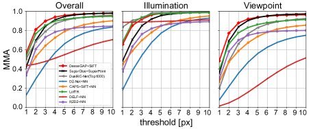
Method #Correspondences D2-Net [27]+NN 2.8K DELF [46]+NN 1.9K R2D2 [26]+NN 1.8K CAPS [14]+SIFT [8]+NN 1.5K DualRC-Net [12](Top1000) 1.0K SuperGlue [5]+SuperPoint [47] 0.9K LofTR [4] 1.8K DenseGAP+SIFT 1.9K

Figure 4: HPatches evaluation. Left: MMA comparison with previous work. Right: The mean number of correspondences for different methods.

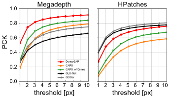
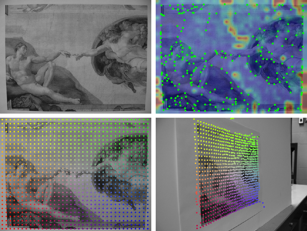
(a) PCK Evaluation	(b) Qualitative Results

Figure 5: Dense geometric matching evaluation. (a) Comparison of PCK scores. (b) Qualitative results on HPatches. Row 1: Left: Input Image, Right: Error map of dense correspondences, and anchor points (colored in green) generated by SuperGlue [5]. We calculate the reprojection errors of each query point and generate the error map using bilinear interpolation. Row 2: Correspondences between two images (indicated by different colors). The error bar on the right is only used for the error map. Note that we use the officially released pretrained model of GOCor [3] and GLU-Net [2] in this experiment.

As shown in Fig. 3, we first initialize local features at coarse and fine levels using a typical convolutional neural network (CNN), denoted as $F^{c}$ and $F^{f}$. Then we compute the features of anchor points by bilinearly interpolating $F^{c}$ and obtain the features $F^{c}_{{\mathcal{A}}_{a}}$ and $F^{c}_{\mathcal{A}_{b}}$ for anchor points in $I_{a}$ and $I_{b}$ respectively. Together with $F^{c}_{a}$ and $F^{c}_{b}$, they form the input of the propagation module, indicating the initial attributes of the nodes in ${\mathcal{V}}_{x}$, ${\mathcal{V}}_{y}$, ${\mathcal{V}}_{a}$, ${\mathcal{V}}_{b}$, which will be updated by the message-passing layers. The propagation module consists of $N_{l}$ intra-points message-passing layers and $N_{l}$ inter-points message-passing layers, followed by one point-to-image message-passing layer. We alternate the inter- and intra-points message-passing layers, starting with one inter-points message-passing layer. In addition, in each of the message-passing layers, we concatenate the node attributes with 2D position embeddings, which are calculated by the 2D sinusoidal position encoding method proposed in [32]. With the unique positional information, the learned features are position-dependent and more robust against matching ambiguity in indistinctive or textureless regions. This module finally outputs two updated coarse features ${F^{c}_{a}}^{\prime}$ and ${F^{c}_{b}}^{\prime}$, and feed them to the refinement module. In the refinement module, we bilinearly upsample ${F^{c}_{a}}^{\prime}$ and ${F^{c}_{b}}^{\prime}$ to fine level, concatenate them with the corresponding fine features and finally feed them to one convolutional layer to generate the result ${F^{f}_{a}}^{\prime}$ and ${F^{f}_{b}}^{\prime}$.

III-D Coarse-to-Fine Training Strategy

Since our network predicts both coarse- and fine-level feature maps, we use a coarse-to-fine matching strategy introduced by [14] to compute the correspondence at a lower resolution followed by a local refinement at a finer scale. Given a query point $x$ in $I_{a}$, we first find its coarse correspondence $y_{c}$ using ${F^{c}_{b}}^{\prime}$ and then crop a local window centered at $y_{c}$ in ${F^{f}_{b}}^{\prime}$, extracting the final correspondence $y$ within the window.

Losses

To train the model given an image pair, we randomly sample the query point $x$ from the pixels that can find ground-truth correspondences on the other image. For the set of training pairs $\mathcal{Q}=\{(x,y_{gt})\}$, the loss function is defined as the error between the established matches and ground-truth correspondence:

$$\mathcal{L}=\sum_{(x,y_{gt})\in\mathcal{Q}}\frac{1}{\sigma_{y}}({\left\lVert y_{gt}-y_{c}\right\rVert}_{2}+{\left\lVert y_{gt}-y\right\rVert}_{2}),$$ (7)

where $\sigma_{y}$ is the uncertainty of the prediction proposed in [14]. Besides, the anchor points are also randomly sampled from the points with known ground-truth correspondence. Meanwhile, we design a grid filter to make them evenly distributed. For more details, please refer to the supplementary material.

Adaptive Position Embedding

When training with fixed-size images, the learned model will degrade when testing with size-free images. To address this problem, we propose a simple and efficient method to augment the pixel coordinates with a random scale for each image. Specifically, in every training iteration, we assign a scale $r_{a}=(r_{a1},r_{a2})$ for $I_{a}$, and $r_{b}=(r_{b1},r_{b2})$ for $I_{b}$. Then, for every point $x=(x_{1},x_{2})$ from $I_{a}$, we scale it to $(x_{1}\cdot r_{a1},x_{2}\cdot r_{a2})$ before feeding it to the position encoder, and apply to $I_{b}$ in the same way. This method significantly improves the result in size-free evaluations.

III-E Runtime Correspondence Prediction

At inference, we first extract anchor points for both input images, and then feed them to our graph-structured network to generate the feature maps. For any query point in $I_{a}$, we use the coarse-to-fine method same as training to compute its correspondence in $I_{b}$. Although the ground-truth correspondence anchor points are used for training, our model adapts well to the anchor points generated by other sparse matching methods when testing. In our experiments, we use SuperGlue [5] to efficiently provide reliable anchor points. Moreover, for any query point, we propose a metric based on cycle consistency to measure the confidence of its correspondence, which is used to filter the matches. The cycle consistency is defined as the euclidean distance between $x$ and $x^{\prime}$ where $x$ is the query point in $I_{a}$ with its correspondence $y$ searched in $I_{b}$ and $x^{\prime}$ is the matching point of $y$ when searching back in $I_{a}$.

IV Experiments

This section starts with training datasets and implementation details, followed by the evaluations of our approach on diverse tasks. Finally, we conduct a comprehensive ablation study of the proposed network structure. For training details and more results, please refer to the supplementary material.

Datasets

Our model is trained with MegaDepth [48] and ScanNet [49] for outdoor and indoor scenes respectively. MegaDepth [48] consists of over 600,000 preprocessed image pairs introduced by CAPS [14]. We follow the same split of 130 scenes for training and 37 for validation. ScanNet is a large-scale indoor dataset, which is split into 1,513 training scenes and 100 testing scenes, same as [5].

Implementation Details

We adopt a modified ResNet-18 [50] as backbone to extract feature maps. We set the number of layers $N_{l}$ to 4 and attention heads to 4 as well. When searching the correspondence in fine-level features, we set the window size as $1/8$ of the feature map size.

IV-A Image Matching

Datasets and Metrics

HPatches is a benchmark dataset with 108 image sequences for evaluating the image matching accuracy. Each sequence contains one query image and five reference images with either changing illumination or viewpoints (52 for illumination and 56 for viewpoint). We use mean matching accuracy (MMA) [27] for evaluating, which is calculated as the percentage of corrected matches in sampled query points within a threshold against ground truth matching.

Results

We use keypoints extracted by SIFT [8] as our query points, filter out all correspondences with cycle consistency larger than 5 pixels, and select top 2,000 matches for each image pair. We compare with R2D2 [26], D2-Net [27], CAPS [14], SuperGlue [5], LofTR [4] and DualRC-Net [12] and show that our model achieves the best overall performance with a large number of correspondences in Fig. 4.

IV-B Geometric Matching

Datasets and Metrics

Both HPatches [51] (viewpoint sequences only) and MegaDepth [48] are used for this evaluation. We use the percentage of correct keypoints (PCK) as the evaluation metric. A correspondence is considered correct if it is close enough (e.g. within a given threshold) to the ground truth. Following  [14], we densely sample correspondences between test image pairs and evaluate the PCK on them.

TABLE I: Pose Estimation Evaluation on the outdoor and indoor datasets. The * indicates the model trained on MegaDepth [48].

Method AUC(5) AUC(10) AUC(20) MegaDepth [48] DualRC-Net [12] 32.56 47.60 61.40 SP [47]+SuperGlue [5] 34.81 50.46 64.43 DenseGAP 41.17 56.87 70.22 ScanNet [49] DualRC-Net [12]* 6.94 17.06 29.58 SP [47]+SuperGlue [5] 16.16 33.81 51.84 DenseGAP* 16.93 34.85 53.16 DenseGAP 17.01 36.07 55.66

Results

We show the results of our model compared to the SOTA methods (GOCor [3], GLU-Net [2] and CAPS [14]) in Fig. 5. For a fair comparison, we also train CAPS  [14] using our loss function, and test it separately (labeled as CAPS w/ Dense). Our model (DenseGAP) significantly outperforms other methods on MegaDepth and achieves a comparable result on HPatches with GOCor [3] and GLU-Net [2]. Both methods we think are naturally well-fit to predict displacements that can be interpolated bilinearly, such as the Homography space in HPatches. However, in a more general scenario with real-world non-planar objects (MegaDepth), DenseGAP outperforms by learning the distinctive features of each query point. Furthermore, while CAPS [14] also uses a similar coarse-to-fine strategy to generate correspondences, DenseGAP achieves significant improvements thanks to the effectiveness of our graph-structured network.

IV-C Relative Pose Estimation

Datasets and Metrics

We evaluate the model using pose estimation on MegaDepth [48] for outdoor scenes and ScanNet [49] for indoor scenes. We randomly select 2,459 image pairs from the validation dataset of MegaDepth and use 1,500 image pairs of ScanNet [49] provided by [5]. We adopt the same evaluation metric as [5], which calculates the area under cumulative error curve (AUC) of pose error up to thresholds ($5^{\circ}$, $10^{\circ}$, $20^{\circ}$). The relative pose is estimated by applying RANSAC [52] on the correspondences.

Results

We compare with the SOTA dense correspondence method DualRC-Net [12] and the SOTA sparse matching method SuperGlue [5] in Tab. I. We use 500 matching pairs of the SuperGlue output as the anchor points, and query the SIFT [8] keypoints and dense points following the same sampling strategy as in Sec IV-B. We filter the matches by selecting the top 8,000 correspondences from the predicted correspondences with cycle consistency larger than 5 pixels. Compared to SuperGlue, our model significantly boosts the performance using denser matches. We attribute this improvement to successfully getting dense correspondences based on sparse priors, which allows us to extract pixel-level image information and fuse them with contextual information from anchor points, thus leading to less biased results.

IV-D Ablation Study

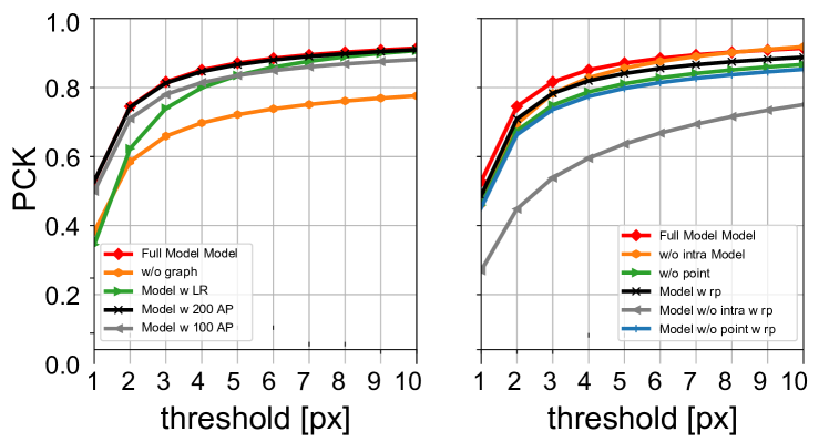
Figure 6: Our model in different settings (left) and using different combinations of message-passing layers (right).

We conduct two ablation studies on MegaDepth with the PCK metric in Fig. 6. We first study the performance of the proposed model under different settings (left). It consists of four variants: (1) Model w/o graph removes the graph-structured representations and only preserves the local feature extractor; (2) Model w/ lower resolution (LR) changes the resolution of feature maps to $1/4$ and $1/16$ of the image size; and (3)&(4) Models w/ 200/100 anchor points(AP) reduce the number of anchor points to 200 and 100, to show the performance of limited anchor points. The first two variants decrease the score in different patterns, which indicates the feasibility and inevitability of our design. Reducing the number of anchor points does not have much effect on the results unless the number is too low, indicating that our model is robust to the number of anchor points. Then we explore the effectiveness of our message-passing layers using two variants of our model under the original setting (right in Fig. 6): (1) Model w/o intra removes the intra-points layer; and (2) Model w/o point removes both intra-points and inter-points layers. Additionally, we test them with a more challenging setting where the locations of $60\%$ of anchor points are interfered with Gaussian noise with standard deviation of 50 pixels (i.e., Model w/o intra w/ rp, Model w/o point w/ rp, Full Model w/ rp). We observe that without the intra-points layer, the model performance is close to the full model in the original setting, but substantially degrades as the outliers increase. The model without inter- and intra-points layers performs obviously worse than the full model due to the lack of cross-image context.

V Conclusion

We propose a novel dense correspondence learning approach that utilizes anchor points with a graph-structured network. The feature descriptors fusing contextual information introduced by anchor points with local information serve for correspondence establishment for any query point and significantly improve the performance on diverse tasks. This model has the potential to generalize to other tasks such as normal estimation, optical flow, etc. An end-to-end solution will be an interesting future direction that jointly optimizes anchor points and dense correspondence.

References

- [1] Iaroslav Melekhov, Aleksei Tiulpin, Torsten Sattler, Marc Pollefeys, Esa Rahtu, and Juho Kannala. Dgc-net: Dense geometric correspondence network. In IEEE Winter Conference on Applications of Computer Vision, WACV 2019, pages 1034–1042. IEEE, 2019.
- [2] Prune Truong, Martin Danelljan, and Radu Timofte. Glu-net: Global-local universal network for dense flow and correspondences. In 2020 IEEE/CVF Conference on Computer Vision and Pattern Recognition, CVPR 2020, pages 6257–6267. IEEE, 2020.
- [3] Prune Truong, Martin Danelljan, Luc Van Gool, and Radu Timofte. Gocor: Bringing globally optimized correspondence volumes into your neural network. In Advances in Neural Information Processing Systems 33: Annual Conference on Neural Information Processing Systems 2020, NeurIPS 2020, 2020.
- [4] Jiaming Sun, Zehong Shen, Yuang Wang, Hujun Bao, and Xiaowei Zhou. LoFTR: Detector-free local feature matching with transformers. CVPR, 2021.
- [5] Paul-Edouard Sarlin, Daniel DeTone, Tomasz Malisiewicz, and Andrew Rabinovich. Superglue: Learning feature matching with graph neural networks. In 2020 IEEE/CVF Conference on Computer Vision and Pattern Recognition, CVPR 2020, pages 4937–4946. IEEE, 2020.
- [6] Qunjie Zhou, Torsten Sattler, and Laura Leal-Taixé. Patch2pix: Epipolar-guided pixel-level correspondences. CoRR, abs/2012.01909, 2020.
- [7] Wei Jiang, Eduard Trulls, Jan Hosang, Andrea Tagliasacchi, and Kwang Moo Yi. COTR: correspondence transformer for matching across images. In 2021 IEEE/CVF International Conference on Computer Vision, ICCV 2021, Montreal, QC, Canada, October 10-17, 2021, pages 6187–6197. IEEE, 2021.
- [8] David G. Lowe. Distinctive image features from scale-invariant keypoints. Int. J. Comput. Vis., 60(2):91–110, 2004.
- [9] Miguel Lourenço, João Pedro Barreto, and Francisco Vasconcelos. srd-sift: Keypoint detection and matching in images with radial distortion. IEEE Trans. Robotics, 28(3):752–760, 2012.
- [10] Ignacio Rocco, Relja Arandjelovic, and Josef Sivic. Efficient neighbourhood consensus networks via submanifold sparse convolutions. In Computer Vision - ECCV 2020, volume 12354 of Lecture Notes in Computer Science, pages 605–621. Springer, 2020.
- [11] Ignacio Rocco, Mircea Cimpoi, Relja Arandjelovic, Akihiko Torii, Tomás Pajdla, and Josef Sivic. Neighbourhood consensus networks. In Advances in Neural Information Processing Systems 31: Annual Conference on Neural Information Processing Systems 2018, NeurIPS 2018, pages 1658–1669, 2018.
- [12] Xinghui Li, Kai Han, Shuda Li, and Victor Prisacariu. Dual-resolution correspondence networks. In Advances in Neural Information Processing Systems 33: Annual Conference on Neural Information Processing Systems 2020, NeurIPS 2020, 2020.
- [13] Shuda Li, Kai Han, Theo W. Costain, Henry Howard-Jenkins, and Victor Prisacariu. Correspondence networks with adaptive neighbourhood consensus. In 2020 IEEE/CVF Conference on Computer Vision and Pattern Recognition, CVPR 2020, Seattle, WA, USA, June 13-19, 2020, pages 10193–10202. IEEE, 2020.
- [14] Qianqian Wang, Xiaowei Zhou, Bharath Hariharan, and Noah Snavely. Learning feature descriptors using camera pose supervision. In Computer Vision - ECCV 2020, volume 12346 of Lecture Notes in Computer Science, pages 757–774. Springer, 2020.
- [15] Axel Barroso Laguna, Edgar Riba, Daniel Ponsa, and Krystian Mikolajczyk. Key.net: Keypoint detection by handcrafted and learned CNN filters. In 2019 IEEE/CVF International Conference on Computer Vision, ICCV 2019, pages 5835–5843. IEEE, 2019.
- [16] Karel Lenc and Andrea Vedaldi. Learning covariant feature detectors. In Computer Vision - ECCV 2016 Workshops, volume 9915 of Lecture Notes in Computer Science, pages 100–117, 2016.
- [17] Dmytro Mishkin, Filip Radenovic, and Jiri Matas. Repeatability is not enough: Learning affine regions via discriminability. In Computer Vision - ECCV 2018, volume 11213 of Lecture Notes in Computer Science, pages 287–304. Springer, 2018.
- [18] Yannick Verdie, Kwang Moo Yi, Pascal Fua, and Vincent Lepetit. TILDE: A temporally invariant learned detector. In IEEE Conference on Computer Vision and Pattern Recognition, CVPR 2015, pages 5279–5288. IEEE Computer Society, 2015.
- [19] Herbert Bay, Tinne Tuytelaars, and Luc Van Gool. SURF: speeded up robust features. In Computer Vision - ECCV 2006, volume 3951 of Lecture Notes in Computer Science, pages 404–417. Springer, 2006.
- [20] Ethan Rublee, Vincent Rabaud, Kurt Konolige, and Gary R. Bradski. ORB: an efficient alternative to SIFT or SURF. In IEEE International Conference on Computer Vision, ICCV 2011, pages 2564–2571. IEEE Computer Society, 2011.
- [21] Stefan Leutenegger, Margarita Chli, and Roland Siegwart. BRISK: binary robust invariant scalable keypoints. In IEEE International Conference on Computer Vision, ICCV 2011, pages 2548–2555. IEEE Computer Society, 2011.
- [22] Kwang Moo Yi, Eduard Trulls, Vincent Lepetit, and Pascal Fua. LIFT: learned invariant feature transform. In Computer Vision - ECCV 2016, volume 9910, pages 467–483. Springer, 2016.
- [23] Anastasya Mishchuk, Dmytro Mishkin, Filip Radenovic, and Jiri Matas. Working hard to know your neighbor’s margins: Local descriptor learning loss. In Advances in Neural Information Processing Systems 30: Annual Conference on Neural Information Processing Systems 2017, pages 4826–4837, 2017.
- [24] Zixin Luo, Tianwei Shen, Lei Zhou, Jiahui Zhang, Yao Yao, Shiwei Li, Tian Fang, and Long Quan. Contextdesc: Local descriptor augmentation with cross-modality context. In IEEE Conference on Computer Vision and Pattern Recognition, CVPR 2019, Long Beach, CA, USA, June 16-20, 2019, pages 2527–2536. Computer Vision Foundation / IEEE, 2019.
- [25] Zixin Luo, Tianwei Shen, Lei Zhou, Siyu Zhu, Runze Zhang, Yao Yao, Tian Fang, and Long Quan. Geodesc: Learning local descriptors by integrating geometry constraints. In Computer Vision - ECCV 2018, volume 11213 of Lecture Notes in Computer Science, pages 170–185. Springer, 2018.
- [26] Jérôme Revaud, César Roberto de Souza, Martin Humenberger, and Philippe Weinzaepfel. R2D2: reliable and repeatable detector and descriptor. In Advances in Neural Information Processing Systems 32: Annual Conference on Neural Information Processing Systems 2019, NeurIPS 2019, pages 12405–12415, 2019.
- [27] Mihai Dusmanu, Ignacio Rocco, Tomás Pajdla, Marc Pollefeys, Josef Sivic, Akihiko Torii, and Torsten Sattler. D2-net: A trainable CNN for joint description and detection of local features. In IEEE Conference on Computer Vision and Pattern Recognition, CVPR 2019, pages 8092–8101. Computer Vision Foundation / IEEE, 2019.
- [28] Daniel DeTone, Tomasz Malisiewicz, and Andrew Rabinovich. Superpoint: Self-supervised interest point detection and description. In 2018 IEEE Conference on Computer Vision and Pattern Recognition Workshops, CVPR Workshops 2018, Salt Lake City, UT, USA, June 18-22, 2018, pages 224–236. IEEE Computer Society, 2018.
- [29] Prune Truong, Martin Danelljan, Luc Van Gool, and Radu Timofte. Learning accurate dense correspondences and when to trust them. In IEEE Conference on Computer Vision and Pattern Recognition, CVPR 2021, virtual, June 19-25, 2021, pages 5714–5724. Computer Vision Foundation / IEEE, 2021.
- [30] Ashish Vaswani, Noam Shazeer, Niki Parmar, Jakob Uszkoreit, Llion Jones, Aidan N. Gomez, Lukasz Kaiser, and Illia Polosukhin. Attention is all you need. In Advances in Neural Information Processing Systems 30: Annual Conference on Neural Information Processing Systems 2017, December 4-9, 2017, Long Beach, CA, USA, pages 5998–6008, 2017.
- [31] Alexey Dosovitskiy, Lucas Beyer, Alexander Kolesnikov, Dirk Weissenborn, Xiaohua Zhai, Thomas Unterthiner, Mostafa Dehghani, Matthias Minderer, Georg Heigold, Sylvain Gelly, Jakob Uszkoreit, and Neil Houlsby. An image is worth 16x16 words: Transformers for image recognition at scale. CoRR, abs/2010.11929, 2020.
- [32] Nicolas Carion, Francisco Massa, Gabriel Synnaeve, Nicolas Usunier, Alexander Kirillov, and Sergey Zagoruyko. End-to-end object detection with transformers. In Computer Vision - ECCV 2020, volume 12346 of Lecture Notes in Computer Science, pages 213–229. Springer, 2020.
- [33] Fuzhi Yang, Huan Yang, Jianlong Fu, Hongtao Lu, and Baining Guo. Learning texture transformer network for image super-resolution. In 2020 IEEE/CVF Conference on Computer Vision and Pattern Recognition, CVPR 2020, pages 5790–5799. IEEE, 2020.
- [34] Ruiyu Li, Makarand Tapaswi, Renjie Liao, Jiaya Jia, Raquel Urtasun, and Sanja Fidler. Situation recognition with graph neural networks. In IEEE International Conference on Computer Vision, ICCV 2017, pages 4183–4192. IEEE Computer Society, 2017.
- [35] Ching-Yao Chuang, Jiaman Li, Antonio Torralba, and Sanja Fidler. Learning to act properly: Predicting and explaining affordances from images. In 2018 IEEE Conference on Computer Vision and Pattern Recognition, CVPR 2018, pages 975–983. IEEE Computer Society, 2018.
- [36] Paul Vicol, Makarand Tapaswi, Lluís Castrejón, and Sanja Fidler. Moviegraphs: Towards understanding human-centric situations from videos. In 2018 IEEE Conference on Computer Vision and Pattern Recognition, CVPR 2018, pages 8581–8590. IEEE Computer Society, 2018.
- [37] Sijie Yan, Yuanjun Xiong, and Dahua Lin. Spatial temporal graph convolutional networks for skeleton-based action recognition. In Proceedings of the Thirty-Second AAAI Conference on Artificial Intelligence, (AAAI-18), pages 7444–7452. AAAI Press, 2018.
- [38] Kfir Aberman, Peizhuo Li, Dani Lischinski, Olga Sorkine-Hornung, Daniel Cohen-Or, and Baoquan Chen. Skeleton-aware networks for deep motion retargeting. ACM Trans. Graph., 39(4):62, 2020.
- [39] Nanyang Wang, Yinda Zhang, Zhuwen Li, Yanwei Fu, Wei Liu, and Yu-Gang Jiang. Pixel2mesh: Generating 3d mesh models from single RGB images. In Computer Vision - ECCV 2018, volume 11215 of Lecture Notes in Computer Science, pages 55–71. Springer, 2018.
- [40] Chao Wen, Yinda Zhang, Zhuwen Li, and Yanwei Fu. Pixel2mesh++: Multi-view 3d mesh generation via deformation. In 2019 IEEE/CVF International Conference on Computer Vision, ICCV 2019, pages 1042–1051. IEEE, 2019.
- [41] Franco Scarselli, Marco Gori, Ah Chung Tsoi, Markus Hagenbuchner, and Gabriele Monfardini. The graph neural network model. IEEE Trans. Neural Networks, 20(1):61–80, 2009.
- [42] Xiaolong Wang, Yufei Ye, and Abhinav Gupta. Zero-shot recognition via semantic embeddings and knowledge graphs. In 2018 IEEE Conference on Computer Vision and Pattern Recognition, CVPR 2018, pages 6857–6866. IEEE Computer Society, 2018.
- [43] Han Hu, Jiayuan Gu, Zheng Zhang, Jifeng Dai, and Yichen Wei. Relation networks for object detection. In 2018 IEEE Conference on Computer Vision and Pattern Recognition, CVPR 2018, pages 3588–3597. IEEE Computer Society, 2018.
- [44] Yue Wang, Yongbin Sun, Ziwei Liu, Sanjay E. Sarma, Michael M. Bronstein, and Justin M. Solomon. Dynamic graph CNN for learning on point clouds. ACM Trans. Graph., 38(5):146:1–146:12, 2019.
- [45] Peter W. Battaglia, Jessica B. Hamrick, Victor Bapst, Alvaro Sanchez-Gonzalez, Vinícius Flores Zambaldi, Mateusz Malinowski, Andrea Tacchetti, David Raposo, Adam Santoro, Ryan Faulkner, Çaglar Gülçehre, H. Francis Song, Andrew J. Ballard, Justin Gilmer, George E. Dahl, Ashish Vaswani, Kelsey R. Allen, Charles Nash, Victoria Langston, Chris Dyer, Nicolas Heess, Daan Wierstra, Pushmeet Kohli, Matthew Botvinick, Oriol Vinyals, Yujia Li, and Razvan Pascanu. Relational inductive biases, deep learning, and graph networks. CoRR, abs/1806.01261, 2018.
- [46] Hyeonwoo Noh, Andre Araujo, Jack Sim, Tobias Weyand, and Bohyung Han. Large-scale image retrieval with attentive deep local features. In IEEE International Conference on Computer Vision, ICCV 2017, pages 3476–3485. IEEE Computer Society, 2017.
- [47] Daniel DeTone, Tomasz Malisiewicz, and Andrew Rabinovich. Superpoint: Self-supervised interest point detection and description. In Proceedings of the IEEE Conference on Computer Vision and Pattern Recognition (CVPR) Workshops, June 2018.
- [48] Zhengqi Li and Noah Snavely. Megadepth: Learning single-view depth prediction from internet photos. In 2018 IEEE Conference on Computer Vision and Pattern Recognition, CVPR 2018, pages 2041–2050. IEEE Computer Society, 2018.
- [49] Angela Dai, Angel X. Chang, Manolis Savva, Maciej Halber, Thomas A. Funkhouser, and Matthias Nießner. Scannet: Richly-annotated 3d reconstructions of indoor scenes. In 2017 IEEE Conference on Computer Vision and Pattern Recognition, CVPR 2017, pages 2432–2443. IEEE Computer Society, 2017.
- [50] Kaiming He, Xiangyu Zhang, Shaoqing Ren, and Jian Sun. Deep residual learning for image recognition. In 2016 IEEE Conference on Computer Vision and Pattern Recognition, CVPR 2016, pages 770–778. IEEE Computer Society, 2016.
- [51] Vassileios Balntas, Karel Lenc, Andrea Vedaldi, and Krystian Mikolajczyk. Hpatches: A benchmark and evaluation of handcrafted and learned local descriptors. In 2017 IEEE Conference on Computer Vision and Pattern Recognition, CVPR 2017, pages 3852–3861. IEEE Computer Society, 2017.
- [52] Martin A. Fischler and Robert C. Bolles. Random sample consensus: A paradigm for model fitting with applications to image analysis and automated cartography. Commun. ACM, 24(6):381–395, 1981.