HVH: Learning a Hybrid Neural Volumetric Representation for
Dynamic Hair Performance Capture

Abstract

Capturing and rendering life-like hair is particularly challenging due to its fine geometric structure, the complex physical interaction and its non-trivial visual appearance. Yet, hair is a critical component for believable avatars. In this paper, we address the aforementioned problems: 1) we use a novel, volumetric hair representation that is composed of thousands of primitives. Each primitive can be rendered efficiently, yet realistically, by building on the latest advances in neural rendering. 2) To have a reliable control signal, we present a novel way of tracking hair on the strand level. To keep the computational effort manageable, we use guide hairs and classic techniques to expand those into a dense hood of hair. 3) To better enforce temporal consistency and generalization ability of our model, we further optimize the 3D scene flow of our representation with multiview optical flow, using volumetric raymarching. Our method can not only create realistic renders of recorded multi-view sequences, but also create renderings for new hair configurations by providing new control signals. We compare our method with existing work on viewpoint synthesis and drivable animation and achieve state-of-the-art results. Please check out our project website at https://ziyanw1.github.io/hvh/.

1 Introduction

Although notable progress has been made towards the realism of human avatars, cephalic hair is still one of the hardest parts of the human body to capture and render: with usually more than a hundred-thousand components, with complex physical interaction among them and with complex interaction with light, which is extraordinarily hard to model. However, it is an important part of our appearance and identity: hair styles can convey everything from religious beliefs to mood or activity. Hence, hair is critically important to make virtual avatars believable and universally usable.

Previous work on mesh based representations [26, 58, 59, 21, 69, 53, 3] has shown promising results on modeling the face and skin. However, they suffer when modeling hair, because meshes are not well suited for representing hair geometry. Recent volumetric representations [27, 36] have high DoF which allows modeling of a changing geometric structure. They have achieved impressive results in 3D scene acquisition and rendering from multi-view photometric information. Compared to other geometric representations like multi-plane images [57, 77, 35, 2, 5] or point-based representations [1, 66, 34, 20, 50], volumetric representations support a larger range of camera motion for view extrapolation and do not suffer from holes when rendering dynamic geometry like point-based representations. Furthermore, they can be learned from multi-view RGB data using differentiable volumetric ray marching, without additional MVS methods.

However, one major flaw of volumetric representations is their cubic memory complexity. This problem is particularly significant for hair, where high resolution is a requirement. NeRF [36] circumvents the $O(n^{3})$ memory complexity problem by parameterizing a volumetric radiance field using an MLP. Given the implicit form, the MLP-based implicit function is not limited by spatial resolution. A hierarchical structure with a coarse and fine level radiance function is used and an importance resampling based on the coarse level radiance field is utilized for boosting sample resolution. Although promising empirical results have been shown, they come with at the advance of high rendering time and the quality is still limited by the coarse level sampling resolution. Another limitation of NeRFs is that they were initially designed for static scenes. There is some recent work [60, 42, 23, 22, 68, 47, 64, 43, 75] that extends the original NeRF concept to modeling dynamic scenes. However, they are still limited to relatively small motions, do not support drivable animation or are not efficient for rendering.

We present a hybrid representation: by using many volumetric primitives, we focus the resolution of the model onto the relevant regions of the 3D space. For each of the volumes, we construct a neural representation that captures the local appearance of the hair in great detail, similar to [25, 64, 48, 28] . However, without explicitly modeling the dynamics and structure of hair, it would be hard for the model to learn these properties solely through the indirect supervision of the multi-view appearance. Given that the model learns to position primitives in an unsupervised manner, the model is also prone to overfitting as a result of not incorporating any temporal consistency during training. We address the problem of spatio-temporal modeling of dynamic upper head and hair by explicitly modeling hair dynamics at the coarse level and by enforcing temporal consistency of the model by multi-view optical flow at the fine level.

Procedurally, we first perform hair strand tracking at a coarse level by lifting multi-view optical flow to a 3D scene flow. To constrain the hair geometry and reduce the impact of the noise in multi-view optical flow, we also make sure the tracked hair strands preserve geometric properties like shape, length and curvature across time. As a second step, we attach volumes to hair strands to model the dynamic scene which can be optimized using differentiable volumetric raymarching. The volumes that are attached to the hair strands are regressed using a decoder that takes per-hair-strand features and a global latent code as input and is aware of the hair specific structure. Additionally, we further enforce fine 3D flow consistency by rendering the 3D scene flow of our model into 2D and compare it with the corresponding ground truth optical flow. This step is essential for making the model generalize better to unseen motions. To summarize, the contributions of this work are

• A hybrid neural volumetric representation that binds volumes to guide hair strands for hair performance capture.

• A hair tracking algorithm that utilizes multiview optical flow and per-frame hair strand reconstruction while preserving specific geometric properties like hair strand length and curvature.

• A volumetric ray marching algorithm on 3D scene flow which enables optimization of the position and orientation of each volumetric primitive through multiview 2D optical flow.

• A hair specific volumetric decoder for hair volume regression and with awareness of hair structure.

2 Related Work

In this section, we discuss the most closely related classical hair dynamic and shape modeling methods. We then discuss learning-based approaches that use either volumetric or non-volumetric scene representations for spatio-temporal modeling.

Image-based Hair Geometry Acquisition is challenging due to the complicated hair geometry, massive number of strands, severe self occlusion and collision and view-dependent appearance. Paris et al. [40, 39] and Wei et al. [65] reconstruct 3D hair geometry from 2D/3D orientation fields using multi-view images. Luo et al. [30, 32] further improve the 3D reconstruction by refining the point cloud from traditional MVS with structure-aware aggregation and strand-based refinement. Luo et al. [31] and Hu et al. [12] progressively fit hair specific structures like ribbons and wisps to the point cloud. Recently, Nam et al. [37] substitute the plane assumption in the conventional MVS by a line-based structure to reconstruct 3D line clouds. Sun et al. [56] use OLAT images for more efficient reconstruction of line-based MVS and develop an inverse rendering pipeline for hair that reasons about hair specific reflectance. However, none of those methods explicitly model temporal consistency for a time series capture.

Dynamic Hair Capture. Compared to the vast body of work on hair geometry acquisition, the work on hair dynamics [11, 76, 70, 72] acquisition is much less. Zhang et al. [76] uses hair simulation to enforce better temporal consistency over a per-frame hair reconstruction result. Hu et al. [11] solves the physics parameters of a hair dynamics model by running parallel processes under different simulation parameters and adopting the one that best matches the visual observation. Xu et al. [70] performs visual tracking by aligning per-frame reconstruction of hair strands with motion paths of hair strands on a horizontal slice of a video volume. Yang et al. [72] developed a deep learning framework for hair tracking using indirect supervision from 2D hair segmentation and a digital 3D hair dataset. However those methods mainly focus on geometry modeling and are not photometrically accurate or do not support drivable animation.

Non-Volumetric Representations are widely studied in the literature of spatio-temporal modeling Mesh-based representations [26, 58, 59, 21, 69, 3] are a perfect fit for modeling surfaces and highly efficient to render. However, they have limitations for modeling complex geometries like hair. Multi-plane images [57, 77, 35, 2, 5] are good at modeling continuous shapes similar to volumetric representations, but are limited to a constrained set of viewing angles. Point cloud representations [1, 66, 34, 20, 50] can model various geometries with high fidelity. When used for appearance modeling, however, point-based representations might suffer from their innate sparseness which might result in holes. Thus image-level rendering techniques [49] are often accompanied with such representations for completeness.

Volumetric Representations are highly flexible and thus can model many different objects. They are designed for geometric completeness given their dense grid-like structure. Many previous works have demonstrated the strength of such representations in geometry modeling [9, 67, 15, 61, 78, 8, 62]. Some recent works [54, 27, 45] have also shown their effectiveness in modeling appearance. DeepVoxels [54] learn a 3D grid of features as the scene representation. Neural volumes [27] learns a grid of discrete color and density values via volumetric raymarching. Neural body [45] incorporates SMPL [29] with Neural Volumes [27] for body modeling. Nevertheless, the rendering quality, efficiency and memory footprint of those volumetric representations is still limited by the voxel resolutions. To conquer this major drawback of volumetric methods, MVP [28] proposes a hybrid representation for efficient and high-fidelity rendering. It attaches a set of local volumetric primitives to a tracked head mesh and employs a tailored volumetric raymarching algorithm that is developed for fast rendering via a BVH [16]. The tracked mesh provides a good initialization for the positions and rotations of the primitives that are jointly learned. Still, finding the globally optimal positions and rotations purely based on a photometric reconstruction loss is highly challenging due to many local minima in the energy formulation.

Coordinate-based Representations have been the major focus of recent literature in 3D learning due to their low memory footprint and ability to dynamically assign the model capacity to the correct regions of 3D space. Many works have demonstrated their ability to reconstruct high fidelity geometry [41, 51, 6, 52, 14, 10, 33, 44] or to generate photo-realistic rendering results [55, 38, 73, 36, 25, 74]. NeRF [36] learns a volumetric radiance field of a static scene from multi-view photometric supervision using a differentiable raymarcher, but comes with a large rendering time. Several works [25, 74, 48, 24] have improved the rendering efficiency of NeRF on static scene. Among all those approaches, the most related to ours are spatio-temporal modeling techniques  [60, 42, 23, 22, 68, 47, 64, 43]. Non-rigid NeRF [60], D-NeRF [47] and Nerfies [42] introduce a dynamic modeling framework with a canonical radiance field and per-frame warpings. Some works [22, 68, 23, 64, 75, 63] model a 3D video by additionally conditioning the radiance field on temporally varying latent codes or an additional time index. Xian et al. [68] further leverages depth as an extra source of supervision. STaR [75] models scenes that consist of a background and one dynamic rigid object. NSFF [23] also combines a static and dynamic NeRF pipeline and uses optical flow to constrain the 3D scene flow derived from the NeRF model of adjacent time frames. Wang et al. [64] introduce a grid of local animation codes for better generalization and improved rendering efficiency. However, these methods are still limited by either sampling resolution or ability to model complex motions and do not generalize well to unseen motions.

3 Method

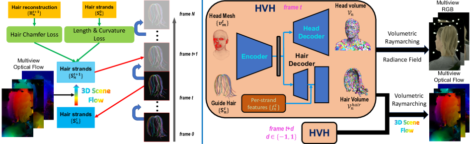
Figure 1: Pipeline. Our method consists of two stages: in the first stage, we perform guide hair tracking with multiview optical flow as well as per-frame hair reconstruction. In the second stage, we further amplify the sparse guide hair strands by attaching volumetric neural rendering primitives and optimizing them by using the multiview RGB and optical flow data.

In this section, we introduce our hybrid neural volumetric representation for hair performance capture. Our representation combines both, the drivability of guide hair strands and the completeness of volumetric primitives. Additionally, the guide hair strands serve as an efficient coarse level geometry for volumetric primitives to attach to, avoiding unnecessary computational expense on empty space. As a result of guide hair strand tracking as well as dense 3D scene flow refinement, our model is temporally consistent with better generalization over unseen motions. As illustrated in Fig. 1, the whole pipeline contains two major steps which we will explain separately. In the first step, we perform strand-level tracking that leverages multi-view optical flow information and propagates information about a subset of tracked hair strands into future frames. To save computation time, we track only guide hairs instead of tracking all hair strands. This is a widely used technique in hair animation and simulation [13, 46, 7], which leads to a significant boost in run time performance. However, getting the guide hairs tracked is not enough to model the hair motion and appearance or to animate all the hairs due to the sparseness of the guide hairs. To circumvent this, we combine it with a volumetric representation by attaching volumetric primitives to the nodes on the guide hairs. This hybrid representation has good localization of hairs in an explicit way and has full coverage of all the hairs, making use of the benefits of both representations. Another advantage is that the introduction of volumes allows optimizing hair shape and appearance by multi-view dense photometric information via differentiable volumetric ray marching. In the second step, we use the attached volumetric primitives to model the hairs that are surrounding the guide hair strands to achieve dense hair appearance, shape and motion acquisition. A hair specific volume decoder is designed for regressing those volumes, conditioning on both a global latent vector and hair strand feature vectors with hair structure awareness. Additionally, we develop a volumetric raymarching algorithm for 3D scene flow that facilitates the learning from multi-view 2D optical flow. We show in the experiments that the introduction of additional optical flow supervision yields better temporal consistency and generalization of the model.

3.1 Guide Hair Tracking

We frame the guide hair tracking process as an optimization problem. Given the guide hair strands and multi-view optical flow at the current frame $t$, we unproject and fuse optical flow under different camera poses into 3D flow and use that to infer the next possible position of the guide hairs at the next frame $t+1$.

Data Setup and Notation. In our setting, we perform hair tracking using multi-view video data. We use a multi-camera system with around 100 synchronized color cameras that produces $2048\times 1334$ resolution images at 30 Hz. The cameras are focused at the center of the capture system and distributed spherically at a distance of one meter to provide as many viewpoints as possible. Camera intrinsics and extrinsics are calibrated in an offline process. We generate multi-view optical flow between adjacent frames for each camera, using the OpenCV [4] implementation of [19]. We acquire per-frame hair geometry by running [37]. We parameterize guide hairs as connected point clouds. Given a specific hair strand $\mathbf{S}^{t}$ at time frame $t$, we denote the Euclidean coordinate of the $\mathbf{n}$th node on hair strand $\mathbf{S}^{t}$ as $\mathbf{S}^{t}_{n}$. Similarly, we have the future position of $\mathbf{S}^{t}_{n}$ at time frame $t+1$ as $\mathbf{S}^{t+1}_{n}$. Next we introduce the notations for multi-view camera related information. We denote $\Pi_{i}(\cdot)$ as the camera transformation matrix of camera $i$ which projects a 3D point into 2D image coordinate. We denote $\mathbf{I}_{of,i}$ and $\mathbf{I}_{d,i}$ as 2D matrix of optical flow and depth of camera $i$ respectively. We denote $\mathbf{H}^{t}_{n}$ as the reconstructed point cloud with direction from [37, 56]. Unless otherwise stated, all bold lower case symbols denote vectors.

Tracking Objectives. Given camera $i$, we could project a 3D point into 2D to retrieve its 2D image index. The camera projection is defined as

$$\mathbf{\hat{p}}^{t}_{s,i}=\begin{bmatrix}\mathbf{p}^{t}_{s,i}\\ \mathbf{1}\end{bmatrix}=\Pi_{i}(\mathbf{S}^{t}_{n}),$$

where $\mathbf{\hat{p}}^{t}_{s,i}$ is the homogeneous coordinate of $\mathbf{p}^{t}_{s,i}$. Given the camera projection formulation, we formulate the first data-term objective based on optical flow as follows:

$$\mathcal{L}_{of} =\sum_{n,i}\mathbf{\omega}_{n,i}||\mathbf{S}^{t+1}_{n}-\mathbf{Z}_{i}(\mathbf{S}^{t+1}_{n})\Pi_{i}^{-1}(\mathbf{p}^{t}_{s,i}+\delta_{\mathbf{p}})||^{2}_{2},$$

$$\mathbf{\omega}_{n,i} =exp(-\sigma||\mathbf{Z}_{i}(\mathbf{S}^{t}_{n})-\mathbf{I}_{d,i}(\mathbf{p}^{t}_{s,i})||^{2}_{2}),$$

$$\delta_{\mathbf{p}} =\mathbf{I}_{of,i}(\mathbf{p}^{t}_{s,i}),$$

where we denote $\mathbf{Z}_{i}(\cdot)$ as the function that represents the depth of a certain point under camera $i$ and $\omega_{i}$ serves as a weighting factor for view selection where a smaller value means larger mismatch of projected depth and real depth under the $i$th camera pose. We use a $\sigma=0.01$.

In parallel with the data-term objective on optical flow, we add another data-term objective to facilitate geometry preserved tracking, which compares the Chamfer distance between tracked guide hair strands and the per-frame hair reconstruction from [37]. This loss is designed to make sure that the guide hair geometry point cloud will not deviate too much from the true hair geometry. Unlike the conventional Chamfer loss, we also penalize the cosine distance between the directions of $\mathbf{S}^{t}_{n}$ and the direction of its closest $k=10$ neighbors as $\mathcal{H}(\mathbf{S}^{t+1}_{n})\subsetneq\{\mathbf{H}^{t+1}_{n}\}$; the losses are defined as:

$$\mathcal{L}_{hdir} =\sum_{n,\mathbf{h}\in\mathcal{H}(\mathbf{S}^{t+1}_{n})}\omega_{n,\mathbf{h}}^{d}(1-|\cos(\mathbf{dir}(\mathbf{S}^{t+1}_{n}),\mathbf{dir}(\mathbf{h}))|),$$

$$\mathcal{L}_{hpos} =\sum_{n,\mathbf{h}\in\mathcal{H}(\mathbf{S}^{t+1}_{n})}\omega_{n,\mathbf{h}}^{r}||\mathbf{S}^{t+1}_{n}-\mathbf{h}||^{2}_{2},$$

where $\omega_{n,\mathbf{h}}^{d}=exp(-\sigma||\mathbf{S}^{t+1}_{n}-\mathbf{h}||^{2}_{2})$ is a spatial weighting, $cos(\cdot,\cdot)$ is a cosine distance function between two vectors and $\mathbf{dir}(\mathbf{S}^{t+1}_{n})=\mathbf{S}^{t+1}_{n+1}-\mathbf{S}^{t+1}_{n}$ is a first order approximation of the hair direction at $\mathbf{S}^{t+1}_{n}$. $\omega_{n,\mathbf{h}}^{r}=cos(\mathbf{dir}(\mathbf{S}^{t+1}_{n}),\mathbf{dir}(\mathbf{h}))$ is a weighting factor that aims at describing the direction similarity between $\mathbf{S}^{t+1}_{n}$ and $\mathbf{h}$. With $\mathcal{L}_{hdir}$, we could groom the guide hairs $\mathbf{S}^{t+1}_{n}$ to have similar direction to its closest $k=10$ neighbors in $\mathcal{H}(\mathbf{S}^{t+1}_{n})$, resulting in a more consistent guide hair direction distribution. Alternatively, $\mathcal{L}_{hpos}$ guarantees that the tracked guide hairs do not deviate too much from the reconstructed hair shapes.

However, with just the data-term loss, the tracked guide hairs might overfit to noise in the data terms. To prevent this, we further introduce several model-term objectives for hair shape regularization.

$$\mathcal{L}_{len}= \sum_{n}(||\mathbf{dir}(\mathbf{S}^{t+1}_{n})||_{2}-||\mathbf{dir}(\mathbf{S}^{0}_{n})||_{2})^{2},$$

$$\mathcal{L}_{tang}= \sum_{n}((\mathbf{S}^{t+1}_{n+1}-\mathbf{S}^{t+1}_{n}-\mathbf{S}^{t}_{n+1}+\mathbf{S}^{t}_{n})\cdot\mathbf{dir}(S^{t}_{n}))^{2}+$$

$$((\mathbf{S}^{t}_{n+1}-\mathbf{S}^{t}_{n}-\mathbf{S}^{t+1}_{n+1}+\mathbf{S}^{t+1}_{n})\cdot\mathbf{dir}(S^{t+1}_{n}))^{2},$$

$$\mathcal{L}_{cur}= \sum_{n}(\mathbf{cur}(\mathbf{S}^{t+1}_{n})-\mathbf{cur}(\mathbf{S}^{0}_{n})),$$

where $\mathbf{cur}(\mathbf{S}^{t}_{n})$ is a numerical approximation of curvature at point $\mathbf{S}^{t}_{n}$ and is defined as:

$$\sqrt{\frac{24(||\mathbf{dir}(\mathbf{S}^{t}_{n})||_{2}+||\mathbf{dir}(\mathbf{S}^{t}_{n})||_{2}-||\mathbf{S}^{t}_{n}-\mathbf{S}^{t}_{n+2}||_{2})}{||\mathbf{S}^{t}_{n}-\mathbf{S}^{t}_{n+2}||_{2}^{3}}}.$$

We optimize all loss terms together to solve $\{\mathbf{S}^{t+1}_{n}\}$ given $\{\mathbf{S}^{t}_{n}\}$ with:

$$\mathcal{L}_{hair}= \mathcal{L}_{of}+\omega_{hdir}\mathcal{L}_{hdir}+\omega_{hpos}\mathcal{L}_{hpos}$$

$$+\omega_{len}\mathcal{L}_{len}+\omega_{tang}\mathcal{L}_{tang}+\omega_{cur}\mathcal{L}_{cur}.$$

By utilizing momentum information across the temporal axis, we can provide a better initialization of $\mathbf{S}^{t+1}_{n}$ given its trajectory and intialize $\mathbf{S}^{t+1}_{n}$ as

$$\mathbf{S}^{t+1}_{n}=3\mathbf{S}^{t}_{n}-3\mathbf{S}^{t-1}_{n}+\mathbf{S}^{t-2}_{n}.$$

3.2 HVH

Background. Similar to MVP, we define volumetric primitives $\mathcal{V}_{n}=\{\mathbf{t}_{n},\mathbf{R}_{n},\mathbf{s}_{n},\mathbf{V}_{n}\}$ to model a volume of local 3D space each, where $\mathbf{R}_{n}\in SO(3),\mathbf{t}_{n}\in\mathbb{R}^{3}$ describes the volume-to-world transformation, $\mathbf{s}_{n}\in\mathbb{R}^{3}$ are the per-axis scale factors and $\mathbf{V}_{n}=[\mathbf{V}_{c},\mathbf{V}_{\alpha}]\in\mathbb{R}^{4\times M\times M\times M}$ is a volumetric grid that stores three channel color and opacity information. The volumes are placed on a UV-map that are unwrapped from a head tracked mesh and are regressed from a 2D CNN. Using an optimized BVH implementation, we can efficiently determine how the rays intersect each volume and find hit boxes. For each ray $\mathbf{r}_{p}(t)=\mathbf{o}_{p}+t\mathbf{d}_{p}$, we denote $(t_{min},t_{max})$ as the start and end point for ray integration. Then, the differentiable aggregation of those volumetric primitives is defined as:

$$\mathcal{I}_{p} =\int_{t_{min}}^{t_{max}}\mathbf{V}_{c}(\mathbf{r}_{p}(t))\frac{dT(t)}{dt}dt,$$

$$T(t) =min(\int_{t_{min}}^{t}\mathbf{V}_{\alpha}(\mathbf{r}_{p}(t))dt,1).$$

We composite the rendered image as $\mathcal{\tilde{I}}_{p}=\mathcal{I}_{p}+(1-\mathcal{A}_{p})I_{p,bg}$ where $\mathcal{A}_{p}=T(t_{max})$ and $I_{p,bg}$ is the background image.

Encoder. The encoder uses the driving signal of a specific point in time and outputs a global latent code $\bm{\mathit{z}}\in\mathbb{R}^{256}$. We use the tracked guide hairs $\{\mathbf{S}_{n}^{t}\}$ and tracked head mesh vertices $\{\bm{v}^{t}_{m}\}$ to define the driving signal. Symmetrically, we learn another decoder in parallel with the encoder in an auto-encoding way that regresses the tracked guide hairs $\{\mathbf{S}_{n}^{t}\}$ and head mesh vertices $\{\bm{v}^{t}_{m}\}$ from the global latent code $\bm{\mathit{z}}$. The architecture of the encoder is an MLP that regresses the parameter of a normal distribution $\mathcal{N}(\bm{\mu},\bm{\sigma}),\bm{\mu},\bm{\sigma}\in\mathcal{R}^{256}$. We use the reparameterization trick from [18] to sample $\bm{\mathit{z}}$ from $\mathcal{N}(\bm{\mu},\bm{\sigma})$ in a differentiable way.

Hair Volume Decoder. Besides the volumes that are attached to the tracked mesh $\{\bm{v}^{t}_{m}\}$, we define additional hair volume $\mathcal{V}_{n}^{hair}$ that are associated with guide hair nodes $\mathbf{S}^{t}_{n}$. The position $\mathbf{t}_{n}=\mathbf{\hat{t}}_{n}+\delta_{\mathbf{t}_{n}}$, orientation $\mathbf{R}_{n}=\delta_{\mathbf{R}_{n}}\cdot\mathbf{\hat{R}}_{n}$ and scale $\mathbf{s}_{n}=\mathbf{\hat{s}}_{n}+\delta_{\mathbf{s}_{n}}$ of each hair volume are determined by the base hair transformation $(\mathbf{\hat{t}}_{n},\mathbf{\hat{R}}_{n},\mathbf{\hat{s}}_{n})$ and regressed hair relative transformation $(\delta_{\mathbf{t}_{n}},\delta_{\mathbf{R}_{n}},\delta_{\mathbf{s}_{n}})$. The base translation $\mathbf{\hat{t}}_{n}$ of each hair node is directly its position $\mathbf{S}_{n}^{t}$. The base rotation $\mathbf{\hat{R}}_{n}$ is derived from the hair tangential direction and the hair-head relative position. We denote $\tau_{n}$ as the hair tnagential direction at position $\mathbf{S}_{n}^{t}$ and $\nu^{\prime}_{n}$ as the direction pointing to the tracked head center starting from $S_{n}^{t}$. Then, the base rotation is $\mathbf{\hat{R}}_{n}=[\tau_{n}^{T};\rho_{n}^{T};\nu_{n}^{T}]$, where $\rho_{n}=\tau_{n}\times\nu^{\prime}_{n},\nu_{n}=\rho_{n}\times\tau_{n}$.

The geometry of hair can not be simply described by a surface. Therefore, we design a 2D CNN that convolves along the hair growing direction and the rough hair spatial position separately. Specifically, in the each layer of the 2D CNN, we seperate a $k\times k$ filter into two $k\times 1$ and $1\times k$ filters and apply convolution along two orthogonal directions respectively, similar to [71]. To learn a more consistent hair shape and appearance model, we optimize per-strand hair features $\{f_{n}^{t}\}$ that are shared across all time frames besides the temporally varying global latent code $\bm{\mathit{z}}$. For each node $\mathbf{S_{n}^{t}}$ on a hair strand $\mathbf{S}^{t}$, we assign an unique feature vector $f^{t}_{n}$. The shared per-strand hair features and the temporal varying latent code $\bm{\mathit{z}}$ are fused to serve as the input to the hair volume decoder, which is shown in Fig. 12.

Figure 2: Architecture of the hair decoder. The hair decoder takes both the global latent code $z$ and the per-strand hair features $\{f_{n}^{t}\}$ as inputs. $z$ is first deconvolved into a 2D feature tensor. It is then padded and concatenated with $\{f_{n}^{t}\}$. In the following operation, the 2D convolution layers are applied along the hair growing direction and the hair spatial position seperately.

Differentiable Volumetric Raymarching of 3D Scene Flow. Learning a volumetric scene representation by multi-view photometric information is sufficient for high fidelity rendering and novel view synthesis. However, it is challenging for the model to reason about motion given the limited supervision and the results have poor temporal consistency, especially on unseen sequences. To better enforce temporal consistency, we develop a differentiable volumetric ray marching algorithm of 3D scene flow which enables training via multi-view 2D optical flow.

Given the transformations of each primitive as $(\mathbf{t}_{n},\mathbf{R}_{n},\mathbf{s}_{n})$, we express the coordinate of each node on a volumetric grid at frame $u$ as $\mathbf{V}_{xyz}^{u}=\mathbf{s}_{t}\mathbf{R}_{t}\mathbf{V}_{tpl}+\mathbf{t}_{n}$, where $\mathbf{V}_{tpl}$ are the coordinates of a 3D mesh grid ranging between $[-1,1]$. Given that the 3D scene flow from frame $u$ to $u+\delta$ can be expressed by each volumetric primitives as $\{\mathbf{\delta V}_{xyz}^{u,u+\epsilon}=\mathbf{V}_{xyz}^{u+\epsilon}-\mathbf{V}_{xyz}^{u}\}$ and rendered into 2D flow as:

$$\mathcal{I}_{p,flow}^{u,u+\delta} =\int_{t_{min}}^{t_{max}}(\mathbf{\delta V}_{xyz}^{u,u+\epsilon}(\mathbf{r}_{p}(t)))\frac{dT(t)}{dt}dt,$$

$$T(t) =min(\int_{t_{min}}^{t_{max}}\mathbf{V}_{\alpha}^{u}(\mathbf{r}_{p}(t))dt,1).$$

Training Objectives. We train our model in an end-to-end manner with the following loss:

$$\mathcal{L}= \mathcal{L}_{pho}+\lambda_{flow}\mathcal{L}_{flow}+\lambda_{geo}\mathcal{L}_{geo}$$

$$+\lambda_{vol}\mathcal{L}_{vol}+\lambda_{cub}\mathcal{L}_{cub}+\lambda_{KL}\mathcal{L}_{KL}.$$

The first term $\mathcal{L}_{pho}$ is the photometric loss that compares the difference between the rendered image $\mathcal{\tilde{I}}_{p}$ and ground truth image $I_{p}$ on all sampled pixels $p\in\mathcal{P}$,

$$\mathcal{L}_{pho}=\sum_{p\in\mathcal{P}}||I_{p,gt}-\mathcal{\tilde{I}}_{p}||^{2}_{2}.$$

The second term $\mathcal{L}_{flow}$ aims to enforce temporal consistency of volumetric primitives from frame $u$ and its adjacent frame $u+\epsilon$ by minimizing the projected 2D flow and ground truth optical flow $I_{p,flow}^{u,u+\epsilon}$,

$$\mathcal{L}_{flow}=\sum_{p\in\mathcal{P}}\mathcal{A}_{p}||I_{p,of}^{u,u+\epsilon}-\mathcal{I}_{p,flow}^{u,u+\epsilon}||^{2}_{2},$$

where $\epsilon\in\{-1,1\}$. It is important to note that we use $\mathcal{A}_{p}$ to mask out the background part and we do not back propagate the errors from $\mathcal{L}_{flow}$ to $\mathcal{A}_{p}$ in order to get rid of the background noise in optical flows. To better enforce hair and head primitives moving with the tracked head mesh and guide hair strands, $\mathcal{L}_{geo}$ is designed to measure the difference between the mesh/strand vertices and their corresponding regressed value.

$$\mathcal{L}_{geo}=\sum_{n}||\bm{S}^{t}_{n}-\bm{S}^{t}_{n,gt}||^{2}_{2}+\sum_{m}||\bm{v}^{t}_{m}-\bm{v}^{t}_{m,gt}||^{2}_{2},$$

where $\bm{S}_{n}^{t}$ and $\bm{v}_{m}^{t}$ are the coordinate of the $n$th node of the tracked guide hair and tracked head mesh at frame $t$ and the $X_{gt}$ denotes the corresponding ground truth value.

We also add several regularization terms to inform the layout of the volumetric primitives:

$$\mathcal{L}_{vol} =\sum_{i=1,\cdots,N_{p}}\prod_{j\in\{x,y,z\}}s_{i}^{j},$$

$$\mathcal{L}_{cub} =\sum_{i=1,\cdots,N_{p}}||max(s_{i}^{x},s_{i}^{y},s_{i}^{z})-min(s_{i}^{x},s_{i}^{y},s_{i}^{z})||,$$

where $N_{p}$ stands for the total number of volumetric primitives and $s_{i}^{x},s_{i}^{y},s_{i}^{z}$ are the three entries of each volumetric primitive’s scale $\bm{s}_{j}$. The two regularization terms aim to prevent each primitive from growing too big while preserving the aspect ratio so that they remain approximately cubic. The last term is the Kullback-Leibler divergence loss $\mathcal{L}_{KL}$ which makes the learnt distribution of latent code $\bm{z}$ smooth and enforces similarity with a normal distribution $\mathcal{N}(0,1)$.

4 Experiments

4.1 Dataset

For each video recorded with our multi camera system, we hold out approximately a quarter of the time frames as test sequence and the rest as training sequence. The test sequence will be used for conducting test experiments of drivable animation. This results in roughly 300 frames for training sequence and 100 frames for testing sequence. Additionally, on the training sequence, we hold out 7 cameras that are distributed around the rear and side view of the head. The captured images are downsampled to $1024\times 667$ resolution for training and testing. We train our model exclusively on the training portion of each sequence with $m=93$ training views.

4.2 Novel View Synthesis

Seq01 Seq02 Seq03 MSE SSIM PSNR MSE SSIM PSNR MSE SSIM PSNR PFNeRF 51.25 0.9269 31.16 103.41 0.8659 28.15 76.59 0.9000 29.50 NSFF 50.13 0.9346 31.21 90.06 0.8885 28.75 83.18 0.8936 29.1 NRNeRF 56.78 0.9231 30.78 132.16 0.8549 27.13 79.83 0.8987 29.33 MVP 47.54 0.9476 31.6 77.23 0.9088 29.62 73.78 0.9224 29.66 Ours 41.89 0.9543 32.17 59.84 0.9275 30.69 71.58 0.9314 29.81

Seq01 Seq02 Seq03 MSE SSIM PSNR MSE SSIM PSNR MSE SSIM PSNR MVP 47.54 0.9476 31.6 77.23 0.9088 29.62 73.78 0.9224 29.66 MVP w/ $\mathcal{L}_{flow}$ 46.49 0.9473 31.69 71.07 0.9107 29.93 75.13 0.9240 29.58 Ours w/o $\mathcal{L}_{flow}$ 43.82 0.9508 31.99 65.98 0.9186 30.27 69.97 0.9359 29.93 Ours 41.89 0.9543 32.17 59.84 0.9275 30.69 71.58 0.9314 29.81 MVP 75.68 0.9200 29.49 85.10 0.9039 29.62 83.76 0.9086 29.16 MVP w/ $\mathcal{L}_{flow}$ 67.86 0.9276 30.00 83.11 0.9037 29.93 80.96 0.9086 29.16 Ours w/o $\mathcal{L}_{flow}$ 71.90 0.9223 29.74 72.74 0.9137 30.27 78.34 0.9198 29.44 Ours 65.96 0.9280 30.09 67.75 0.9208 30.69 75.66 0.9222 29.57

Table 1: Novel view synthesis. On the left, we compare our method with both NeRF stemmed methods like NSFF[23], NRNeRF [60] and a per-frame NeRF(PFNeRF) baseline, and a volumetric method like MVP [28]. On the right, we further compare our method and different variants of our methods with MVP on novel views of both seen (top) and unseen (bottom) sequences.

We show both qualitative and quantitative comparisons with other methods [28, 60, 23] on the novel view synthesis task. In the left of Tab. 1, we show the mean squared error(MSE), SSIM and PSNR between predicted images and ground truth images from the novel views of the training sequences. Qualitative results are shown in Fig. 3. Our method has smaller image prediction errors and is able to generate sharper results, especially on the hair regions.

NSFF [23]	NRNeRF [60]	MVP [28]	Ours	Ground Truth

Figure 3: Comparison on novel view synthesis between different methods. Please see supplementary material for a bigger version of this figure.

4.3 Ablation Studies

Temporal consistency. To test the effects of the temporal consistency and the tracked guide hair, we also conduct a novel view synthesis task on the test portion of our captured sequence. Note that our model is not trained using any part of the test sequence data. On the right of Tab. 1, we report MSE, SSIM, PSNR on novel views of both seen and unseen sequences. As we can see, having the coarse level guide hair strands tracked and without flow supervision gives us better rendering quality. With flow supervision, the results are improved further. This improvement is because the tracking information helps the volumetric primitives to better localize the hair region with higher consistency. While the improvement for seen motions is relatively small, both our model and MVP are notably improved for unseen sequences with novel hair motion when flow supervision is added. Rendering results on unseen sequences are shown in Fig. 4. In Fig. 5, we visualize the volumetric primitives of the hairs of our model with and without flow supervision. Including flow supervision produces notably better disentanglement between the hair and shoulder.

MVP

MVP w/ flow

Ours w/o flow

Ours

Ground Truth

Figure 4: Ablation of temporal consistency. We compare our method and MVP w/ and w/o flow supervision. With flow supervision, better temporal consistency and generalization for unseen sequence can be observed. Please see supplementary for a bigger version of this figure.

w/o flow sup.

w/ flow sup.

Ground truth

Figure 5: Ablation on flow supervision. We further compare the volumetric primitives of the models w/ and w/o flow supervision. We see that model with additional flow supervision yields a consistent and reasonable shape for hair and yields better hair shoulder disentanglement.

Hair tracking analysis. We first study the impact of different objectives $\mathcal{L}_{len}+\mathcal{L}_{tang}$ and $\mathcal{L}_{cur}$ in hair tracking. As in Fig. 6, when both $\mathcal{L}_{cur}$ and $\mathcal{L}_{len}+\mathcal{L}_{tang}$ are applied, the tracking results are more smooth and without kinks. We observe that, when using the loss $\mathcal{L}_{len}+\mathcal{L}_{tang}$ as the only regularization term, the length of each hair strand segments are already preserved but could cause some kinks without awareness of the correct hair strand curvatures. $\mathcal{L}_{cur}$ itself does not help and exaggerates the error when the hair strand length is not correct, but yields smooth results when combined with $\mathcal{L}_{len}+\mathcal{L}_{tang}$. This is because curvature computation is agnostic to absolute length of the hair and only controls the relative length ratio.

w/o $\mathcal{L}_{cur}$ $\mathcal{L}_{len}+\mathcal{L}_{tang}$	w/o $\mathcal{L}_{len}+\mathcal{L}_{tang}$	w/o $\mathcal{L}_{cur}$	w/ $\mathcal{L}_{cur}$ $\mathcal{L}_{len}+\mathcal{L}_{tang}$

Figure 6: Effects of $\mathcal{L}_{len}+\mathcal{L}_{tang}$ and $\mathcal{L}_{cur}$. We show how the shape and curvature of tracked hair strands are preserved with both $\mathcal{L}_{len}+\mathcal{L}_{tang}$ and $\mathcal{L}_{cur}$.

We show the impact of different initialization for hair tracking in Fig. 7. When no momentum information from previous frames is used, there is more obvious drifting on some of the strands happening, while the drifting is less severe when we take advantage of the motion information from previous frames.

	frame 118	frame 119	frame 120	frame 121	frame 122
no mm.
1st ord. mm.
2nd ord. mm.

Figure 7: Ablation of different initialization in hair tracking. We show tracking results of our methods with different initializations. From top to bottom, we use no momentum information, first and second order momentum information for tracking initialization. Please note the brown and orange strands. As we can see, the hairs are better tracked when we utilize the dynamic information from previous frames. Better view in color version.

5 Applications and Limitations

One major application that is enabled by our neural volumetric scene representation is novel view synthesis as we have shown in Sec. 4.2. Our neural volumetric representation is also animatable with a sparse driving signals like guide hair strands. Given that we have explicitly modeled hair in the form of guide strands, our method allows modifying the guide hairs directly. In Fig. 8, we show four snapshots of different configurations of hair positions. Please see more results and details in the supplementary material.

Figure 8: Hair position editing. We create a new animation by direct editing on the guide hair strands. As we can see the volumes of hair are driven by the lifted guide hair to create a new hair motion. Please see supplementary material for video results.

There are several limitations of our work which we plan to address in the future: 1) Our method requires the help from artist to prepare guide hair at the first frame and some flyaway hair might be excluded. 2) We currently do not consider physics based interactions between hair and other objects like the shoulder or the chair. 3) Although we achieved certain level of disentanglement between hair and other objects without any human labeling, it is still not perfect. We only showed results on blonde hair which could be better distinguished from a dark background. Our method might be limited by other hairstyles. Future directions like incorporating a physics aware module or leveraging additional supervision from semantic information for disentanglement could be interesting.

6 Discussion

In this paper, we present a hybrid neural volumetric representation for hair dynamic performance capture. Our representation leverages the efficiency of guide hair representation in hair simulation by attaching volumetric primitives to them as well as the high DoF of volumetric representation. With both hair tracking and 3D scene flow refinement, our model enjoys better temporal consistency. We empirically show that our method generates sharper and higher quality results on hair and our method achieves better generalization. Our model also supports multiple applications like drivable animation and hair editing.

7 Appendix

7.1 Dataset and Capture system

We use a multi-camera system with around 100 synchronized color cameras that produces $2048\times 1334$ resolution images at 30 Hz. The cameras are focused at the center of the capture system and distributed spherically at a distance of one meter to provide as many viewpoints as possible. Camera intrinsics and extrinsics are calibrated in an offline process. We captured three sequences of different hair styles and hair motions. In the first sequence, we have one actor with a short high pony tail performing nodding and rotating. In the second sequence, we have one actor with a curly long releasing style hair and leaning her head towards four directions(left, right, up and down) and rotating. In the third sequence, we have one actor with a long high pony tail performing nodding and rotating.

7.2 Baselines

We compare against several volume-based or implicit function based baseline methods [28, 60, 23] for spatio-temporal modeling.

MVP[28] presents an efficient 4D representation for dynamic scenes with humans which is capable of doing animation and novel view synthesis. It combines explicitly tracked head mesh with volumetric primitives to model the human appearance and geometry with better completeness. The volumetric primitives can be aligned onto an unwrapped 2D UV-map from a tracked head mesh and can be regressed from a 2D convolutional neural network that leverages shared spatially computation. Similar to Neural Volumes [27], a differentiable volumetric ray marching algorithm is designed to render 2D rgb images on MVP in real time. We use $N_{p}=4096$ volumetric primitives with a voxel resolution $8\times 8\times 8$ on each sequence with a ray marching step size around $dt=1mm$. We use a global latent size of $256$.

Non-rigid NeRF[60] presents an implicit function based representation for dynamic scene reconstruction and novel view synthesis based on NeRF [36]. It utilizes a hierarchical model by disentangling a dynamic scene into a canonical frame NeRF and its corresponding deformation field which is parameterized by another MLP. In our experiments, we use 128 sampling points for both coarse and fine level sampling. We use the original implementation from the authors  here. We train different models for each sequences and each model is trained for at least 300k iterations until convergence.

NSFF[23] is another implicit function based representation for dynamic scenes that is also based on NeRF [36]. It learns a per-frame NeRF that is additionally conditioned on the time index. It brings optical flow as additional supervision and learns a 3D scene flow in parallel with the per-frame NeRF for enforcing temporal consistency. NSFF is able to perform both spatial and temporal interpolation on a given video sequence. We use a setting of 256 sampling points in our experiments, using [19] as a substitute for generating optical flow. We use the original implementation from the authors  here. We train different models for each sequences and each model is trained for at least 300k iterations until convergence.

7.3 Training Details

For both tracking optimization and HVH training, We deploy Adam [17] for optimization. For hair tracking, we use a learning rate of $1$. We set the weighting coefficients of each losses as $\omega_{hdir}=3$, $\omega_{hpos}=1$, $\omega_{len}=3$, $\omega_{tang}=3$ and $\omega_{cur}=1e4$. For each time step, 100 iterations are taken for optimization to solve the possible hair strands at next frame out. For HVH, we set weighting parameters for each objective as $\lambda_{flow}=1$. $\lambda_{geo}=0.1$, $\lambda_{vol}=0.01$, $\lambda_{cub}=0.01$ and $\lambda_{KL}=0.001$. All models are trained with approximately 100-150k iterations. We use a latent code size of 256 and per-strand hair code size of 256, raymarching step size around $dt=1mm$ and around $N_{p}=5500$ volumetric primitives with a voxel resolution $8\times 8\times 8$ for each sequence depending on the number of guide hairs. For each sequence, we have roughly 30 strands for guide hair and we sample 50 points on each strands.

7.4 Novel View Synthesis

We show a larger version of comparison figure between different methods in Figure 9. For completeness, we also include visualizations from a perframe NeRF model which takes a perframe temporal code as input liker non-rigid NeRF [60].

Perframe NeRF

NSFF [23]

Non-rigid NeRF [60]

MVP [28]

Ours

Ground Truth

Figure 9: Comparison on novel view synthesis between different methods.

7.5 Ablation Studies

Temporal Consistency. We show a bigger version of rendering results on unseen sequence in Figure 10.

MVP

MVP w/ flow

Ours w/o flow

Ours

Ground Truth

Figure 10: Ablation of temporal consistency. We compare MVP [28] and ours with different variations.

Hair Decoder structure. As part of the hair decoder ablation, we compare our method with a naive decoder that uses the same volume decoder as MVP [28] for hair volumes. There are two major differences: 1) the naive decoder does not take the per-strand hair feature as input; 2) The design of the naive decoder does not take into account the hair specific structure where it regresses the same slab as for head tracked mesh and we take the first $N_{hair}$ volumes as the output. In this way, the naive decoder discards all intrinsic geometric structural information while doing convolutions in each layers. We show the hair volumes layout in Figure 11. In the naive design, the hair strands are randomly squeezed into a square UV-map which could break the inner connections of each hair. In our design, we groom the hair strands into the their directions which could preserve the hair specific geometric structure. We compare different designs of decoder on Seq01. As in Table 2, our hair structure aware decoder produces a smaller image reconstruction error and better SSIM, a result of inductive bias of the designed hair decoder.

decoder	MSE	SSIM	PSNR
naive	45.68/75.15	0.9549/0.9220	31.83/29.54
early fus.	43.75/71.08	0.9533/0.9259	31.97/29.82
late fus.	41.89/65.96	0.9543/0.9280	32.17/30.09

Table 2: Decoder structure. We compare different designs of the hair decoder. We report all metrics on both training and testing and we use a to separate them where on the left are the results of novel synthesis on training sequence.

Naive Decoder	Our Decoder

Figure 11: Hair volumes layout. We show the hair volume layout of both naive decoder and ours.

We additionally compare two different designs of the hair decoder where we do late and early fusion of the per-strand hair feature and the global latent feature. We show two different designs in Figure 12. Table 2 shows that the late fusion model performs better than early fusion model. This could be because the late fusion model transfers the 1d global latent code into a spatially varying feature tensor which is a more expressive form of feature representation.

Figure 12: Architecture of the hair decoder. We show late fusion on the top and early fusion on the bottom. The late fusion model first deconvolves the 1D global latent code into a 2D feature map and then concatenate it with the per-strand hair features. A 2D CNN is used afterwards to generate the hair volumes. The early fusion model first repeat the 1D global latent vector spatially and then concatenate the repeated feature map with per-strand hair features. The concatenated features are than fed into a deeper 2D CNN to generate the hair volumes.

7.6 Visualization of Flow

Please see Figure 13 for a visualization of the rendered flow from our representation. Compared to the optical flow from  [19], our rendered 2D flow has less noise on the background. This is because that we only define our 3D scene flow on the volumetric primitives instead of the whole space. With the help of the coarse level geometry like the hair strands and head tracked mesh, the scene flow of most part of the empty space will naturally be zero. This could help us eliminate the noise from the background optical flow to certain degree.

Run Time Analysis. We report the rendering time of one iamge at resolution $1024\times 667$ for each methods here. MVP [28] takes 0.223s. Ours takes 0.254s. NSFF takes 28.68s. NRNeRF [60] takes 41.29s. All tests are conducted under a single Nvidia Tesla V100 GPU.

Flow from ours

Flow from  [19]

Ground truth

Figure 13: Visualization of flow. We show the rendered 3D scene flow into 2D flow in the first column and the openCV optical flow [19] in the second column. The last column shows the ground truth image as reference.

7.7 Hair Tracking Analysis

In Figure 14, we plot different hair properties over time. We report four different metrics describing how well the tracked hairs fit the per-frame reconstruction and how well it preserves its length and curvature. In the first two rows, we report the MSE between the tracked hair and the tracked hair at first frame in terms of curvature and length. In the last two rows, we report the cosine distance between the direction of each nodes on the tracked guide hair and the direction of its neighbor from the reconstruction and the Chamfer distance between the tracked guide hair nodes and the reconstruction. As we can see the length and curvature are relatively preserved across frames and the affinity between the per-frame reconstruction and the tracked guide hair is relatively high.

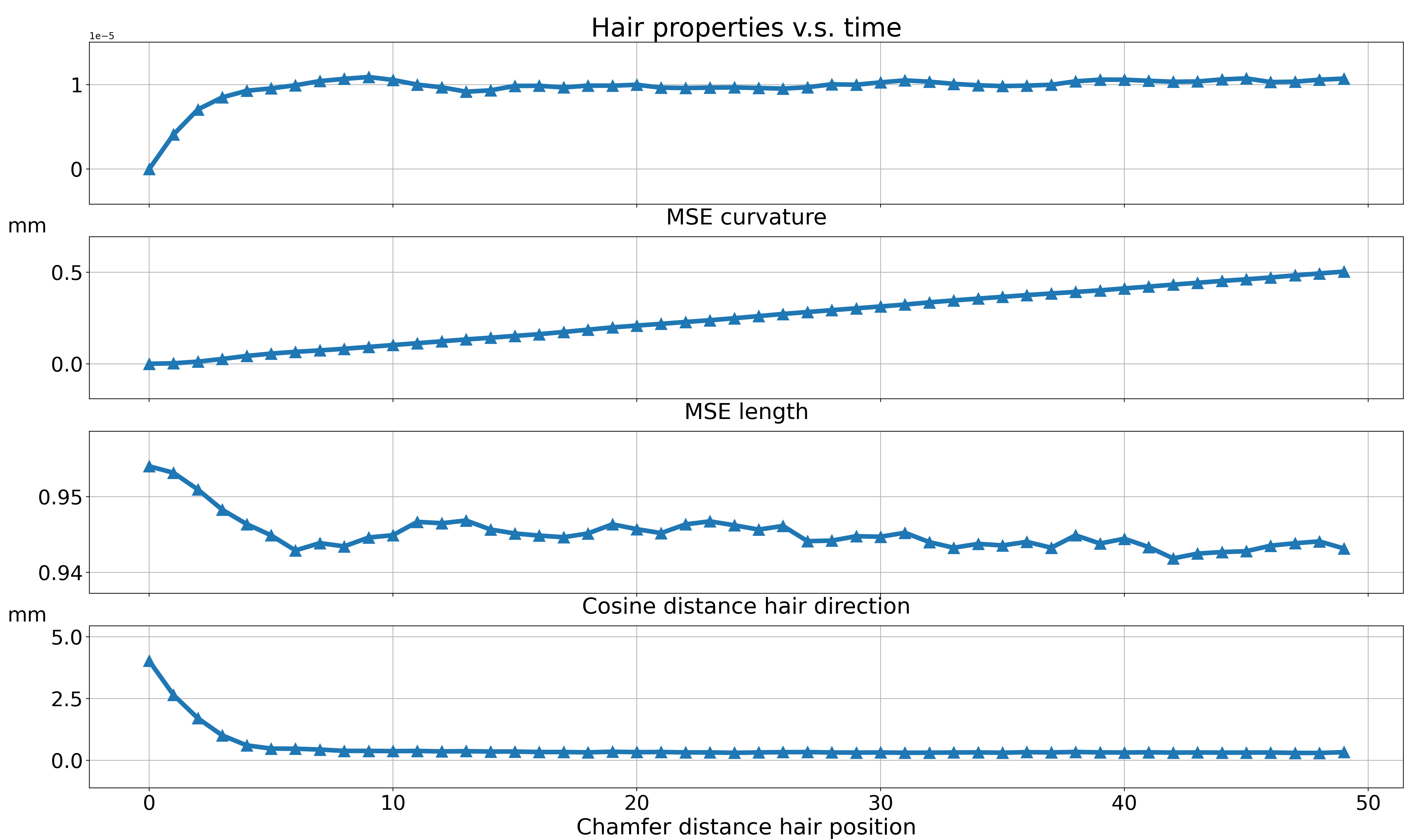
Figure 14: Plot of tracked hair properties v.s. time. As we can see, the hair properties like length and curvature are not changing too much across time and hair Chamfer distance are relatively small.

8 Video Results

Please see all the video results at appended html page: $./video\_navigation/index.html$

References

- [1] Kara-Ali Aliev, Artem Sevastopolsky, Maria Kolos, Dmitry Ulyanov, and Victor Lempitsky. Neural point-based graphics. In European conference on computer vision, pages 696–712. Springer, 2020.
- [2] Benjamin Attal, Selena Ling, Aaron Gokaslan, Christian Richardt, and James Tompkin. Matryodshka: Real-time 6dof video view synthesis using multi-sphere images. In European Conference on Computer Vision, pages 441–459. Springer, 2020.
- [3] Timur Bagautdinov, Chenglei Wu, Tomas Simon, Fabian Prada, Takaaki Shiratori, Shih-En Wei, Weipeng Xu, Yaser Sheikh, and Jason Saragih. Driving-signal aware full-body avatars. ACM Transactions on Graphics (TOG), 40(4):1–17, 2021.
- [4] Gary Bradski. The opencv library. Dr. Dobb’s Journal: Software Tools for the Professional Programmer, 25(11):120–123, 2000.
- [5] Michael Broxton, John Flynn, Ryan Overbeck, Daniel Erickson, Peter Hedman, Matthew Duvall, Jason Dourgarian, Jay Busch, Matt Whalen, and Paul Debevec. Immersive light field video with a layered mesh representation. ACM Transactions on Graphics (TOG), 39(4):86–1, 2020.
- [6] Rohan Chabra, Jan E Lenssen, Eddy Ilg, Tanner Schmidt, Julian Straub, Steven Lovegrove, and Richard Newcombe. Deep local shapes: Learning local sdf priors for detailed 3d reconstruction. In European Conference on Computer Vision, pages 608–625. Springer, 2020.
- [7] Menglei Chai, Changxi Zheng, and Kun Zhou. Adaptive skinning for interactive hair-solid simulation. IEEE transactions on visualization and computer graphics, 23(7):1725–1738, 2016.
- [8] Ricson Cheng, Ziyan Wang, and Katerina Fragkiadaki. Geometry-aware recurrent neural networks for active visual recognition. In S. Bengio, H. Wallach, H. Larochelle, K. Grauman, N. Cesa-Bianchi, and R. Garnett, editors, Advances in Neural Information Processing Systems, volume 31. Curran Associates, Inc., 2018.
- [9] Christopher B Choy, Danfei Xu, JunYoung Gwak, Kevin Chen, and Silvio Savarese. 3d-r2n2: A unified approach for single and multi-view 3d object reconstruction. In European conference on computer vision, pages 628–644. Springer, 2016.
- [10] Kyle Genova, Forrester Cole, Avneesh Sud, Aaron Sarna, and Thomas Funkhouser. Local deep implicit functions for 3d shape. In Proceedings of the IEEE/CVF Conference on Computer Vision and Pattern Recognition, pages 4857–4866, 2020.
- [11] Liwen Hu, Derek Bradley, Hao Li, and Thabo Beeler. Simulation-ready hair capture. In Computer Graphics Forum, volume 36, pages 281–294. Wiley Online Library, 2017.
- [12] Liwen Hu, Chongyang Ma, Linjie Luo, and Hao Li. Robust hair capture using simulated examples. ACM Transactions on Graphics (TOG), 33(4):1–10, 2014.
- [13] Hayley Iben, Mark Meyer, Lena Petrovic, Olivier Soares, John Anderson, and Andrew Witkin. Artistic simulation of curly hair. In Proceedings of the 12th ACM SIGGRAPH/Eurographics Symposium on Computer Animation, pages 63–71, 2013.
- [14] Chiyu Jiang, Avneesh Sud, Ameesh Makadia, Jingwei Huang, Matthias Nießner, Thomas Funkhouser, et al. Local implicit grid representations for 3d scenes. In Proceedings of the IEEE/CVF Conference on Computer Vision and Pattern Recognition, pages 6001–6010, 2020.
- [15] Abhishek Kar, Christian Häne, and Jitendra Malik. Learning a multi-view stereo machine. arXiv preprint arXiv:1708.05375, 2017.
- [16] Tero Karras and Timo Aila. Fast parallel construction of high-quality bounding volume hierarchies. In Proceedings of the 5th High-Performance Graphics Conference, pages 89–99, 2013.
- [17] Diederik P Kingma and Jimmy Ba. Adam: A method for stochastic optimization. arXiv preprint arXiv:1412.6980, 2014.
- [18] Diederik P Kingma and Max Welling. Auto-encoding variational bayes. arXiv preprint arXiv:1312.6114, 2013.
- [19] Till Kroeger, Radu Timofte, Dengxin Dai, and Luc Van Gool. Fast optical flow using dense inverse search. In European Conference on Computer Vision, pages 471–488. Springer, 2016.
- [20] Christoph Lassner and Michael Zollhöfer. Pulsar: Efficient sphere-based neural rendering. In IEEE/CVF Conference on Computer Vision and Pattern Recognition (CVPR), June 2021.
- [21] Tianye Li, Timo Bolkart, Michael J Black, Hao Li, and Javier Romero. Learning a model of facial shape and expression from 4d scans. ACM Trans. Graph., 36(6):194–1, 2017.
- [22] Tianye Li, Mira Slavcheva, Michael Zollhoefer, Simon Green, Christoph Lassner, Changil Kim, Tanner Schmidt, Steven Lovegrove, Michael Goesele, and Zhaoyang Lv. Neural 3d video synthesis. arXiv preprint arXiv:2103.02597, 2021.
- [23] Zhengqi Li, Simon Niklaus, Noah Snavely, and Oliver Wang. Neural scene flow fields for space-time view synthesis of dynamic scenes. In Proceedings of the IEEE/CVF Conference on Computer Vision and Pattern Recognition, pages 6498–6508, 2021.
- [24] David B Lindell, Julien NP Martel, and Gordon Wetzstein. Autoint: Automatic integration for fast neural volume rendering. In Proceedings of the IEEE/CVF Conference on Computer Vision and Pattern Recognition, pages 14556–14565, 2021.
- [25] Lingjie Liu, Jiatao Gu, Kyaw Zaw Lin, Tat-Seng Chua, and Christian Theobalt. Neural sparse voxel fields. In H. Larochelle, M. Ranzato, R. Hadsell, M. F. Balcan, and H. Lin, editors, Advances in Neural Information Processing Systems, volume 33, pages 15651–15663. Curran Associates, Inc., 2020.
- [26] Stephen Lombardi, Jason Saragih, Tomas Simon, and Yaser Sheikh. Deep appearance models for face rendering. ACM Trans. Graph., 37(4), July 2018.
- [27] Stephen Lombardi, Tomas Simon, Jason Saragih, Gabriel Schwartz, Andreas Lehrmann, and Yaser Sheikh. Neural volumes: Learning dynamic renderable volumes from images. ACM Trans. Graph., 38(4), July 2019.
- [28] Stephen Lombardi, Tomas Simon, Gabriel Schwartz, Michael Zollhoefer, Yaser Sheikh, and Jason Saragih. Mixture of volumetric primitives for efficient neural rendering. ACM Trans. Graph., 40(4), July 2021.
- [29] Matthew Loper, Naureen Mahmood, Javier Romero, Gerard Pons-Moll, and Michael J Black. Smpl: A skinned multi-person linear model. ACM transactions on graphics (TOG), 34(6):1–16, 2015.
- [30] Linjie Luo, Hao Li, Sylvain Paris, Thibaut Weise, Mark Pauly, and Szymon Rusinkiewicz. Multi-view hair capture using orientation fields. In 2012 IEEE Conference on Computer Vision and Pattern Recognition, pages 1490–1497. IEEE, 2012.
- [31] Linjie Luo, Hao Li, and Szymon Rusinkiewicz. Structure-aware hair capture. ACM Transactions on Graphics (TOG), 32(4):1–12, 2013.
- [32] Linjie Luo, Cha Zhang, Zhengyou Zhang, and Szymon Rusinkiewicz. Wide-baseline hair capture using strand-based refinement. In Proceedings of the IEEE Conference on Computer Vision and Pattern Recognition, pages 265–272, 2013.
- [33] Lars Mescheder, Michael Oechsle, Michael Niemeyer, Sebastian Nowozin, and Andreas Geiger. Occupancy networks: Learning 3d reconstruction in function space. In Proceedings of the IEEE/CVF Conference on Computer Vision and Pattern Recognition, pages 4460–4470, 2019.
- [34] Moustafa Meshry, Dan B Goldman, Sameh Khamis, Hugues Hoppe, Rohit Pandey, Noah Snavely, and Ricardo Martin-Brualla. Neural rerendering in the wild. In Proceedings of the IEEE/CVF Conference on Computer Vision and Pattern Recognition, pages 6878–6887, 2019.
- [35] Ben Mildenhall, Pratul P Srinivasan, Rodrigo Ortiz-Cayon, Nima Khademi Kalantari, Ravi Ramamoorthi, Ren Ng, and Abhishek Kar. Local light field fusion: Practical view synthesis with prescriptive sampling guidelines. ACM Transactions on Graphics (TOG), 38(4):1–14, 2019.
- [36] Ben Mildenhall, Pratul P Srinivasan, Matthew Tancik, Jonathan T Barron, Ravi Ramamoorthi, and Ren Ng. Nerf: Representing scenes as neural radiance fields for view synthesis. In European conference on computer vision, pages 405–421. Springer, 2020.
- [37] Giljoo Nam, Chenglei Wu, Min H Kim, and Yaser Sheikh. Strand-accurate multi-view hair capture. In Proceedings of the IEEE/CVF Conference on Computer Vision and Pattern Recognition, pages 155–164, 2019.
- [38] Michael Niemeyer, Lars Mescheder, Michael Oechsle, and Andreas Geiger. Differentiable volumetric rendering: Learning implicit 3d representations without 3d supervision. In Proceedings of the IEEE/CVF Conference on Computer Vision and Pattern Recognition, pages 3504–3515, 2020.
- [39] Sylvain Paris, Hector M Briceno, and François X Sillion. Capture of hair geometry from multiple images. ACM transactions on graphics (TOG), 23(3):712–719, 2004.
- [40] Sylvain Paris, Will Chang, Oleg I Kozhushnyan, Wojciech Jarosz, Wojciech Matusik, Matthias Zwicker, and Frédo Durand. Hair photobooth: geometric and photometric acquisition of real hairstyles. ACM Trans. Graph., 27(3):30, 2008.
- [41] Jeong Joon Park, Peter Florence, Julian Straub, Richard Newcombe, and Steven Lovegrove. Deepsdf: Learning continuous signed distance functions for shape representation. In Proceedings of the IEEE/CVF Conference on Computer Vision and Pattern Recognition, pages 165–174, 2019.
- [42] Keunhong Park, Utkarsh Sinha, Jonathan T Barron, Sofien Bouaziz, Dan B Goldman, Steven M Seitz, and Ricardo Martin-Brualla. Nerfies: Deformable neural radiance fields. In Proceedings of the IEEE/CVF International Conference on Computer Vision, pages 5865–5874, 2021.
- [43] Keunhong Park, Utkarsh Sinha, Peter Hedman, Jonathan T. Barron, Sofien Bouaziz, Dan B Goldman, Ricardo Martin-Brualla, and Steven M. Seitz. Hypernerf: A higher-dimensional representation for topologically varying neural radiance fields. arXiv preprint arXiv:2106.13228, 2021.
- [44] Songyou Peng, Michael Niemeyer, Lars Mescheder, Marc Pollefeys, and Andreas Geiger. Convolutional occupancy networks. In Computer Vision–ECCV 2020: 16th European Conference, Glasgow, UK, August 23–28, 2020, Proceedings, Part III 16, pages 523–540. Springer, 2020.
- [45] Sida Peng, Yuanqing Zhang, Yinghao Xu, Qianqian Wang, Qing Shuai, Hujun Bao, and Xiaowei Zhou. Neural body: Implicit neural representations with structured latent codes for novel view synthesis of dynamic humans. In Proceedings of the IEEE/CVF Conference on Computer Vision and Pattern Recognition, pages 9054–9063, 2021.
- [46] Lena Petrovic, Mark Henne, and John Anderson. Volumetric methods for simulation and rendering of hair. Tech. Rep. Pixar Animation Studios, 2(4), 2005.
- [47] Albert Pumarola, Enric Corona, Gerard Pons-Moll, and Francesc Moreno-Noguer. D-nerf: Neural radiance fields for dynamic scenes. In Proceedings of the IEEE/CVF Conference on Computer Vision and Pattern Recognition, pages 10318–10327, 2021.
- [48] Christian Reiser, Songyou Peng, Yiyi Liao, and Andreas Geiger. Kilonerf: Speeding up neural radiance fields with thousands of tiny mlps. In International Conference on Computer Vision (ICCV), 2021.
- [49] Olaf Ronneberger, Philipp Fischer, and Thomas Brox. U-net: Convolutional networks for biomedical image segmentation. In International Conference on Medical image computing and computer-assisted intervention, pages 234–241. Springer, 2015.
- [50] Darius Rückert, Linus Franke, and Marc Stamminger. Adop: Approximate differentiable one-pixel point rendering. arXiv preprint arXiv:2110.06635, 2021.
- [51] Shunsuke Saito, Zeng Huang, Ryota Natsume, Shigeo Morishima, Angjoo Kanazawa, and Hao Li. Pifu: Pixel-aligned implicit function for high-resolution clothed human digitization. In Proceedings of the IEEE/CVF International Conference on Computer Vision, pages 2304–2314, 2019.
- [52] Shunsuke Saito, Tomas Simon, Jason Saragih, and Hanbyul Joo. Pifuhd: Multi-level pixel-aligned implicit function for high-resolution 3d human digitization. In Proceedings of the IEEE/CVF Conference on Computer Vision and Pattern Recognition, pages 84–93, 2020.
- [53] Shunsuke Saito, Jinlong Yang, Qianli Ma, and Michael J Black. Scanimate: Weakly supervised learning of skinned clothed avatar networks. In Proceedings of the IEEE/CVF Conference on Computer Vision and Pattern Recognition, pages 2886–2897, 2021.
- [54] Vincent Sitzmann, Justus Thies, Felix Heide, Matthias Nießner, Gordon Wetzstein, and Michael Zollhofer. Deepvoxels: Learning persistent 3d feature embeddings. In Proceedings of the IEEE/CVF Conference on Computer Vision and Pattern Recognition, pages 2437–2446, 2019.
- [55] Vincent Sitzmann, Michael Zollhöfer, and Gordon Wetzstein. Scene representation networks: Continuous 3d-structure-aware neural scene representations. arXiv preprint arXiv:1906.01618, 2019.
- [56] Tiancheng Sun, Giljoo Nam, Carlos Aliaga, Christophe Hery, and Ravi Ramamoorthi. Human hair inverse rendering using multi-view photometric data. 2021.
- [57] Richard Szeliski and Polina Golland. Stereo matching with transparency and matting. In 6th International Conference on Computer Vision, pages 517–524. IEEE, 1998.
- [58] Ayush Tewari, Michael Zollhofer, Hyeongwoo Kim, Pablo Garrido, Florian Bernard, Patrick Perez, and Christian Theobalt. Mofa: Model-based deep convolutional face autoencoder for unsupervised monocular reconstruction. In Proceedings of the IEEE International Conference on Computer Vision Workshops, pages 1274–1283, 2017.
- [59] Luan Tran and Xiaoming Liu. Nonlinear 3d face morphable model. In Proceedings of the IEEE conference on computer vision and pattern recognition, pages 7346–7355, 2018.
- [60] Edgar Tretschk, Ayush Tewari, Vladislav Golyanik, Michael Zollhöfer, Christoph Lassner, and Christian Theobalt. Non-rigid neural radiance fields: Reconstruction and novel view synthesis of a dynamic scene from monocular video. In IEEE International Conference on Computer Vision (ICCV). IEEE, 2021.
- [61] Shubham Tulsiani, Tinghui Zhou, Alexei A Efros, and Jitendra Malik. Multi-view supervision for single-view reconstruction via differentiable ray consistency. In Proceedings of the IEEE conference on computer vision and pattern recognition, pages 2626–2634, 2017.
- [62] Hsiao-Yu Fish Tung, Ricson Cheng, and Katerina Fragkiadaki. Learning spatial common sense with geometry-aware recurrent networks. In Proceedings of the IEEE/CVF Conference on Computer Vision and Pattern Recognition, pages 2595–2603, 2019.
- [63] Chaoyang Wang, Ben Eckart, Simon Lucey, and Orazio Gallo. Neural trajectory fields for dynamic novel view synthesis, 2021.
- [64] Ziyan Wang, Timur Bagautdinov, Stephen Lombardi, Tomas Simon, Jason Saragih, Jessica Hodgins, and Michael Zollhofer. Learning compositional radiance fields of dynamic human heads. In Proceedings of the IEEE/CVF Conference on Computer Vision and Pattern Recognition (CVPR), pages 5704–5713, June 2021.
- [65] Yichen Wei, Eyal Ofek, Long Quan, and Heung-Yeung Shum. Modeling hair from multiple views. In ACM SIGGRAPH 2005 Papers, pages 816–820. 2005.
- [66] Olivia Wiles, Georgia Gkioxari, Richard Szeliski, and Justin Johnson. Synsin: End-to-end view synthesis from a single image. In Proceedings of the IEEE/CVF Conference on Computer Vision and Pattern Recognition, pages 7467–7477, 2020.
- [67] Jiajun Wu, Chengkai Zhang, Tianfan Xue, William T Freeman, and Joshua B Tenenbaum. Learning a probabilistic latent space of object shapes via 3d generative-adversarial modeling. In Proceedings of the 30th International Conference on Neural Information Processing Systems, pages 82–90, 2016.
- [68] Wenqi Xian, Jia-Bin Huang, Johannes Kopf, and Changil Kim. Space-time neural irradiance fields for free-viewpoint video. In Proceedings of the IEEE/CVF Conference on Computer Vision and Pattern Recognition, pages 9421–9431, 2021.
- [69] Donglai Xiang, Fabian Prada, Chenglei Wu, and Jessica Hodgins. Monoclothcap: Towards temporally coherent clothing capture from monocular rgb video. In 2020 International Conference on 3D Vision (3DV), pages 322–332. IEEE, 2020.
- [70] Zexiang Xu, Hsiang-Tao Wu, Lvdi Wang, Changxi Zheng, Xin Tong, and Yue Qi. Dynamic hair capture using spacetime optimization. To appear in ACM TOG, 33:6, 2014.
- [71] Gengshan Yang and Deva Ramanan. Volumetric correspondence networks for optical flow. In H. Wallach, H. Larochelle, A. Beygelzimer, F. d'Alché-Buc, E. Fox, and R. Garnett, editors, Advances in Neural Information Processing Systems, volume 32. Curran Associates, Inc., 2019.
- [72] Lingchen Yang, Zefeng Shi, Youyi Zheng, and Kun Zhou. Dynamic hair modeling from monocular videos using deep neural networks. ACM Transactions on Graphics (TOG), 38(6):1–12, 2019.
- [73] Lior Yariv, Yoni Kasten, Dror Moran, Meirav Galun, Matan Atzmon, Ronen Basri, and Yaron Lipman. Multiview neural surface reconstruction by disentangling geometry and appearance. arXiv preprint arXiv:2003.09852, 2020.
- [74] Alex Yu, Ruilong Li, Matthew Tancik, Hao Li, Ren Ng, and Angjoo Kanazawa. Plenoctrees for real-time rendering of neural radiance fields. arXiv preprint arXiv:2103.14024, 2021.
- [75] Wentao Yuan, Zhaoyang Lv, Tanner Schmidt, and Steven Lovegrove. Star: Self-supervised tracking and reconstruction of rigid objects in motion with neural rendering. In Proceedings of the IEEE/CVF Conference on Computer Vision and Pattern Recognition, pages 13144–13152, 2021.
- [76] Qing Zhang, Jing Tong, Huamin Wang, Zhigeng Pan, and Ruigang Yang. Simulation guided hair dynamics modeling from video. In Computer Graphics Forum, volume 31, pages 2003–2010. Wiley Online Library, 2012.
- [77] Tinghui Zhou, Richard Tucker, John Flynn, Graham Fyffe, and Noah Snavely. Stereo magnification: Learning view synthesis using multiplane images. ACM Trans. Graph., 37(4), July 2018.
- [78] Rui Zhu, Hamed Kiani Galoogahi, Chaoyang Wang, and Simon Lucey. Rethinking reprojection: Closing the loop for pose-aware shape reconstruction from a single image. In Proceedings of the IEEE Conference on Computer Vision and Pattern Recognition, pages 57–65, 2017.