Bounds on quantum adiabaticity in driven many-body systems
from generalized orthogonality catastrophe and quantum speed limit

Abstract

We provide two inequalities for estimating adiabatic fidelity in terms of two other more handily calculated quantities, i.e., generalized orthogonality catastrophe and quantum speed limit. As a result of considering a two-dimensional subspace spanned by the initial ground state and its orthogonal complement, our method leads to stronger bounds on adiabatic fidelity than those previously obtained. One of the two inequalities is nearly sharp when the system size is large, as illustrated using a driven Rice-Mele model, which represents a broad class of quantum many-body systems whose overlap of different instantaneous ground states exhibits orthogonality catastrophe.

Introduction.— The celebrated quantum adiabatic theorem (QAT) is a fundamental theorem in quantum mechanics Born (1927); Born and Fock (1928); Kato (1950); Messiah (2014), which has many applications ranging from the Gell-Mann and Low formula in quantum field theory Nenciu and Rasche (1989); Fetter and Walecka (2003), Born-Oppenheimer approximation in atomic physics Born and Oppenheimer (1927); Ziman (2001); Car and Parrinello (1985), and adiabatic transport in solid-state physics Thouless (1983); Berry (1984); Avron et al. (1988); Avron (1995) to adiabatic quantum computation Farhi et al. (2000); Roland and Cerf (2002); Albash and Lidar (2018) and adiabatic quantum state manipulation Ivanov (2001); Budich and Trauzettel (2013) in quantum technology. In its simplest form, the QAT states that if the initial state of a quantum system is one of the eigenstates of a time-dependent Hamiltonian, which describes the system, and if the time variation of the Hamiltonian is slow enough, then the state of the system at a later time will still be close to the instantaneous eigenstate of the Hamiltonian. To be more specific, we are interested in the time-dependent Hamiltonian $H^{\,}_{\lambda}$ whose dependence on time $t$ is through an implicit function $\lambda(t).$ For each $\lambda,$ the instantaneous ground state $|\Phi^{\,}_{\lambda}\rangle$ obeys the instantaneous eigenvalue equation of $H^{\,}_{\lambda}$,

$$H^{\,}_{\lambda}|\Phi^{\,}_{\lambda}\rangle=E^{(0)}_{\lambda}|\Phi^{\,}_{\lambda}\rangle,$$ (1)

with $E^{(0)}_{\lambda}$ being the instantaneous ground state energy, whereas the physical state $|\Psi^{\,}_{\lambda}\rangle$ is the solution to the scaled time-dependent Schrödinger equation ($\hbar\equiv 1$),

$$\mathrm{i}\Gamma\frac{\partial}{\partial\lambda}|\Psi^{\,}_{\lambda}\rangle=H^{\,}_{\lambda}|\Psi^{\,}_{\lambda}\rangle,$$ (2)

with $|\Psi^{\,}_{0}\rangle=|\Phi^{\,}_{0}\rangle$ by preparing the initial state, $|\Psi^{\,}_{0}\rangle$, to be the same as the ground state of $H^{\,}_{\lambda=0}$, $|\Phi^{\,}_{0}\rangle.$ Here, $\Gamma\,\raisebox{0.85pt}{.}\raisebox{2.85pt}{.}\!\!=\,\partial^{\,}_{t}\lambda$ is the driving rate.

Mathematically, the QAT states that for however small $\epsilon>0$ and arbitrary value of $\lambda$, there exists a driving rate $\Gamma$ small enough such that

$$1-\mathcal{F}(\lambda)\,<\,\epsilon,$$ (3)

where the fidelity of adiabatic evolution (for short, adiabatic fidelity),

$$\mathcal{F}(\lambda)=|\langle\Phi^{\,}_{\lambda}|\Psi^{\,}_{\lambda}\rangle|^{2},$$ (4)

is the fidelity between the physical state $|\Psi^{\,}_{\lambda}\rangle$ and the instantaneous ground state $|\Phi^{\,}_{\lambda}\rangle$. The QAT is a powerful asymptotic statement. However, in certain contexts, it is not sufficient because one would like to know how quickly $\mathcal{F}(\lambda)$ approaches unity with decreasing the driving rate. This is generally a hard problem since it is difficult to compute the adiabatic fidelity (4) for generic quantum many-body systems by directly solving the instantaneous eigenvalue equation (1) and the time-dependent Schrödinger equation (2). Moreover, most of the existing literature merely proves the existence of the QAT in various settings Kato (1950); Avron et al. (1987); Avron and Elgart (1999); Jansen et al. (2007); Bachmann et al. (2017) but rarely provides useful and practical tools for computing the adiabatic fidelity (4) quantitatively.

To make further progress, an insight proposed in Ref. Lychkovskiy et al. (2017) is to compare the physical state $|\Psi^{\,}_{\lambda}\rangle$ and the instantaneous ground state $|\Phi^{\,}_{\lambda}\rangle$ for a given $\lambda$ with their common initial state $|\Psi^{\,}_{0}\rangle=|\Phi^{\,}_{0}\rangle.$ We now introduce these two extra ingredients in turn. First, the fidelity between the instantaneous ground state $|\Phi^{\,}_{\lambda}\rangle$ and its initial state $|\Phi^{\,}_{0}\rangle$,

$$\mathcal{C}(\lambda)\,\raisebox{0.85pt}{.}\raisebox{2.85pt}{.}\!\!=\,|\langle\Phi^{\,}_{\lambda}|\Phi^{\,}_{0}\rangle|^{2},$$ (5)

is referred to as generalized orthogonality catastrophe. This name is motivated by Anderson’s orthogonality catastrophe Anderson (1967); Gebert et al. (2014), which states that the overlap between ground states in Fermi gases with and without local scattering potentials vanishes as the system size approaches infinity. In a later section, we are interested in a wide range of classes of time-dependent many-body Hamiltonians whose generalized orthogonality catastrophe $\mathcal{C}(\lambda)$ decays exponentially with the system size and $\lambda^{2}$. Second, the fidelity between the physical state $|\Psi^{\,}_{\lambda}\rangle$ and its initial state $|\Psi^{\,}_{0}\rangle$,

$$F(\Psi^{\,}_{\lambda},\Psi^{\,}_{0})\,\raisebox{0.85pt}{.}\raisebox{2.85pt}{.}\!\!=\,|\langle\Psi^{\,}_{\lambda}|\Psi^{\,}_{0}\rangle|^{2},$$ (6)

is another useful quantity since the corresponding Bures angle $D(\Psi^{\,}_{\lambda},\Psi^{\,}_{0})$ Nielsen and Chuang (2010); Bengtsson and Życzkowski (2017),

$$D(\Psi^{\,}_{\lambda},\Psi^{\,}_{0})\,\raisebox{0.85pt}{.}\raisebox{2.85pt}{.}\!\!=\,\frac{2}{\pi}\arccos\sqrt{F(\Psi^{\,}_{\lambda},\Psi^{\,}_{0})},$$ (7)

is upper bounded by using a version of the quantum speed limit Pfeifer (1993); Pfeifer and Fröhlich (1995) ,

$$\frac{\pi}{2}D(\Psi^{\,}_{\lambda},\Psi^{\,}_{0})\leq\min\left(\mathcal{R}(\lambda),\frac{\pi}{2}\right)\equiv\widetilde{\mathcal{R}}(\lambda),$$ (8a)

where

$$\mathcal{R}(\lambda)\,\raisebox{0.85pt}{.}\raisebox{2.85pt}{.}\!\!=\,\int^{\lambda}_{0}\frac{\mathrm{d}\lambda^{\prime}}{|\partial^{\,}_{t}\lambda^{\prime}|}\Delta E^{\,}_{0}(\lambda^{\prime}),$$ (8b)

$$\Delta E^{\,}_{0}(\lambda^{\prime})\,\raisebox{0.85pt}{.}\raisebox{2.85pt}{.}\!\!=\,\sqrt{\langle\Psi^{\,}_{0}|H^{2}_{\lambda^{\prime}}|\Psi^{\,}_{0}\rangle-\langle\Psi^{\,}_{0}|H^{\,}_{\lambda^{\prime}}|\Psi^{\,}_{0}\rangle^{2}}.$$ (8c)

Note that in Eq. (8a) we have taken into account the fact that the Bures angle $D\left(\Psi^{\,}_{\lambda},\Psi^{\,}_{0}\right)\in[0,1]$ by its definition as the function $\mathcal{R}(\lambda)$ defined in Eq. (8b) is not guaranteed to be upper bounded by $\pi/2.$ The quantum speed limit is essentially a measure of how fast a quantum system can evolve. Since the Bures angle $D(\Psi^{\,}_{\lambda},\Psi^{\,}_{0})$ measures a distance between two states, the quantum uncertainty $\Delta E^{\,}_{0}(\lambda^{\prime})$ in Eq. (8) plays the role of speed. Although there is not one single quantum speed limit, we work with the version shown in Eq. (8b) that enables its computation by knowing merely the Hamiltonian and the initial state. It is worth mentioning that a recent theoretical study del Campo (2021) suggests that quantum speed limits can be probed in cold-atom experiments.

Utilizing the generalized orthogonality catastrophe (5) and the quantum speed limit (8) as additional ingredients, the main result of Ref. Lychkovskiy et al. (2017) is an inequality providing an upper bound for the difference between the adiabatic fidelity $\mathcal{F}(\lambda)$ (4) and the generalized orthogonality catastrophe $\mathcal{C}(\lambda)$ (5),

$$\left|\mathcal{F}(\lambda)-\mathcal{C}(\lambda)\right| \;\leq\;\widetilde{\mathcal{R}}(\lambda),$$ (9)

where $\widetilde{\mathcal{R}}(\lambda)$ is defined in Eq. (8a). In this work, we derive two improved inequalities that are stronger than the inequality (9). A schematic summary of our main results is illustrated in Fig. 1.

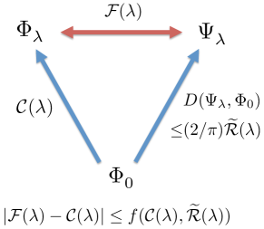
Figure 1: (Color online) Schematic illustration of the relation between the physical state $|\Psi^{\,}_{\lambda}\rangle$, the instantaneous ground state $|\Phi^{\,}_{\lambda}\rangle,$ and the initial state $|\Psi^{\,}_{0}\rangle=|\Phi^{\,}_{0}\rangle.$ The central object is the fidelity between $|\Psi^{\,}_{\lambda}\rangle$ and $|\Phi^{\,}_{\lambda}\rangle$, i.e., $\mathcal{F}(\lambda)$ (4), which can be estimated through $\left|\mathcal{F}(\lambda)-\mathcal{C}(\lambda)\right|\leq f(\mathcal{C}(\lambda),\widetilde{\mathcal{R}}(\lambda)),$ where $f(\mathcal{C}(\lambda),\widetilde{\mathcal{R}}(\lambda))\in$ $\{\widetilde{\mathcal{R}}(\lambda),\;\sin\widetilde{\mathcal{R}}(\lambda),g(\lambda)\}$ from Eqs. (9), (20), and (22).

Derivation of improved inequalities.— In this section, we develop an approach involving two orthonormal vectors to derive inequalities that are stronger than the one in Eq. (9). Observe that for every given $\lambda$, there are three state vectors involved (see also Fig. 1), i.e., $|\Phi^{\,}_{0}\rangle,$ $|\Psi^{\,}_{\lambda}\rangle,$ and $|\Phi^{\,}_{\lambda}\rangle.$ Of which, only $|\Phi^{\,}_{0}\rangle$ is time independent and is still present at a different value of $\lambda$. Therefore, a natural strategy is to decompose the other two states, $|\Psi^{\,}_{\lambda}\rangle$ and $|\Phi^{\,}_{\lambda}\rangle$, into the initial ground state $|\Phi^{\,}_{0}\rangle$ and its orthogonal complement (think of the Gram-Schmidt process). Let $|\Phi^{\perp}_{0}(\lambda)\rangle$ be a $\lambda$-dependent normalized state that is orthogonal to the initial state $|\Phi^{\,}_{0}\rangle,$ i.e., $\langle\Phi^{\,}_{0}|\Phi^{\perp}_{0}(\lambda)\rangle=0,$ we then decompose the physical state $|\Psi^{\,}_{\lambda}\rangle$ in terms of these two orthonormal states,

$$|\Psi^{\,}_{\lambda}\rangle=e^{\mathrm{i}\varphi^{\,}_{\lambda}}\cos\theta^{\,}_{\lambda}|\Phi^{\,}_{0}\rangle+\sin\theta^{\,}_{\lambda}|\Phi^{\perp}_{0}(\lambda)\rangle,$$ (10)

where $\theta^{\,}_{\lambda}\in[0,\pi/2]$ and $\varphi^{\,}_{\lambda}\in[0,2\pi]$ with the subscript $\lambda$ indicates that both $\theta^{\,}_{\lambda}$ and $\varphi^{\,}_{\lambda}$ are a function of $\lambda=\lambda(t)$. Notice that, by construction,

$$|\langle\Phi^{\,}_{0}|\Psi^{\,}_{\lambda}\rangle|=\cos\theta^{\,}_{\lambda}\quad\Leftrightarrow\quad\theta^{\,}_{\lambda}=\frac{\pi}{2}D(\Psi^{\,}_{\lambda},\Psi^{\,}_{0}),$$ (11a)

$$\langle\Phi^{\perp}_{0}(\lambda)|\Psi^{\,}_{\lambda}\rangle=\sin\theta^{\,}_{\lambda}=\sin\left(\frac{\pi}{2}D(\Psi^{\,}_{\lambda},\Psi^{\,}_{0})\right).$$ (11b)

Similarly, the instantaneous ground state $|\Phi^{\,}_{\lambda}\rangle$ can be decomposed into the initial state $|\Phi^{\,}_{0}\rangle$ and another $\lambda$-dependent orthogonal complement $|\widetilde{\Phi}^{\perp}_{0}(\lambda)\rangle$ [which need not be the same as $|\Phi^{\perp}_{0}(\lambda)\rangle$ introduced in Eq. (10)],

$$|\Phi^{\,}_{\lambda}\rangle=\langle\Phi^{\,}_{0}|\Phi^{\,}_{\lambda}\rangle|\Phi^{\,}_{0}\rangle+\langle\widetilde{\Phi}^{\perp}_{0}(\lambda)|\Phi^{\,}_{\lambda}\rangle|\widetilde{\Phi}^{\perp}_{0}(\lambda)\rangle.$$ (12)

The normalization condition, $1=\langle\Phi^{\,}_{\lambda}|\Phi^{\,}_{\lambda}\rangle$, then implies

$$|\langle\widetilde{\Phi}^{\perp}_{0}(\lambda)|\Phi^{\,}_{\lambda}\rangle|=\sqrt{1-|\langle\Phi^{\,}_{0}|\Phi^{\,}_{\lambda}\rangle|^{2}}=\sqrt{1-\mathcal{C}(\lambda)},$$ (13)

where $\mathcal{C}(\lambda)$ is defined in Eq. (5).

Since the components of the physical state $|\Psi^{\,}_{\lambda}\rangle$ (10) are entirely determined by the Bures angle, $D(\Psi^{\,}_{\lambda},\Psi^{\,}_{0})=(2/\pi)\theta^{\,}_{\lambda}$, and that of the instantaneous ground state $|\Phi^{\,}_{\lambda}\rangle$ (12) by the generalized orthogonality catastrophe, $\mathcal{C}(\lambda),$ it is then obvious that their overlap, the adiabatic fidelity $\mathcal{F}(\lambda)$ (4), should be wholly determined by both $\theta^{\,}_{\lambda}$ and $\mathcal{C}(\lambda)$, as will be seen shortly.

We are in a position to compute the adiabatic fidelity $\mathcal{F}(\lambda)$ (4) using Eq. (10),

$$\mathcal{F}(\lambda)=\cos^{2}\theta^{\,}_{\lambda}|\langle\Phi^{\,}_{\lambda}|\Phi^{\,}_{0}\rangle|^{2}+\sin^{2}\theta^{\,}_{\lambda}|\langle\Phi^{\,}_{\lambda}|\Phi^{\perp}_{0}(\lambda)\rangle|^{2}$$

$$+\Re\Big{(}e^{\mathrm{i}\varphi^{\,}_{\lambda}}\sin(2\theta^{\,}_{\lambda})\langle\Phi^{\,}_{\lambda}|\Phi^{\,}_{0}\rangle\langle\Phi^{\perp}_{0}(\lambda)|\Phi^{\,}_{\lambda}\rangle\Big{)}.$$ (14)

The main object of interest, $|\mathcal{F}(\lambda)-\mathcal{C}(\lambda)|,$ can then be computed using (i) Eq. (14), (ii) the triangle inequality for absolute value, and (iii) the inequality $\Re(z)\leq|z|$ for $z\in\mathbb{C}$,

$$\left|\mathcal{F}(\lambda)-\mathcal{C}(\lambda)\right|$$

$$\stackrel{{\scriptstyle\rm(i)}}{{=}} \,\Big{|}\sin^{2}\theta^{\,}_{\lambda}\left(-|\langle\Phi^{\,}_{\lambda}|\Phi^{\,}_{0}\rangle|^{2}+|\langle\Phi^{\,}_{\lambda}|\Phi^{\perp}_{0}(\lambda)\rangle|^{2}\right)$$

$$+\Re\Big{(}e^{\mathrm{i}\varphi^{\,}_{\lambda}}\sin(2\theta^{\,}_{\lambda})\langle\Phi^{\,}_{\lambda}|\Phi^{\,}_{0}\rangle\langle\Phi^{\perp}_{0}(\lambda)|\Phi^{\,}_{\lambda}\rangle\Big{)}\Big{|}$$

$$\stackrel{{\scriptstyle\rm(ii)}}{{\leq}} \,\Big{|}\sin^{2}\theta^{\,}_{\lambda}\left(-|\langle\Phi^{\,}_{\lambda}|\Phi^{\,}_{0}\rangle|^{2}+|\langle\Phi^{\,}_{\lambda}|\Phi^{\perp}_{0}(\lambda)\rangle|^{2}\right)\Big{|}$$

$$+\Big{|}\Re\Big{(}e^{\mathrm{i}\varphi^{\,}_{\lambda}}\sin(2\theta^{\,}_{\lambda})\langle\Phi^{\,}_{\lambda}|\Phi^{\,}_{0}\rangle\langle\Phi^{\perp}_{0}(\lambda)|\Phi^{\,}_{\lambda}\rangle\Big{)}\Big{|}$$

$$\stackrel{{\scriptstyle\rm(iii)}}{{\leq}} \,\Big{|}\sin^{2}\theta^{\,}_{\lambda}\left(-|\langle\Phi^{\,}_{\lambda}|\Phi^{\,}_{0}\rangle|^{2}+|\langle\Phi^{\,}_{\lambda}|\Phi^{\perp}_{0}(\lambda)\rangle|^{2}\right)\Big{|}$$

$$+\sin(2\theta^{\,}_{\lambda})\left|\langle\Phi^{\,}_{\lambda}|\Phi^{\,}_{0}\rangle\right|\left|\langle\Phi^{\perp}_{0}(\lambda)|\Phi^{\,}_{\lambda}\rangle\right|$$

$$\leq \,\Big{|}\sin^{2}\theta^{\,}_{\lambda}\left(-|\langle\Phi^{\,}_{\lambda}|\Phi^{\,}_{0}\rangle|^{2}+|\langle\Phi^{\,}_{\lambda}|\widetilde{\Phi}^{\perp}_{0}(\lambda)\rangle|^{2}\right)\Big{|}$$

$$+\sin(2\theta^{\,}_{\lambda})\left|\langle\Phi^{\,}_{\lambda}|\Phi^{\,}_{0}\rangle\right|\left|\langle\widetilde{\Phi}^{\perp}_{0}(\lambda)|\Phi^{\,}_{\lambda}\rangle\right|,$$ (15)

where the last expression is obtained after using the following inequality,

$$|\langle\Phi^{\perp}_{0}(\lambda)|\Phi^{\,}_{\lambda}\rangle|\;\leq\;|\langle\widetilde{\Phi}^{\perp}_{0}(\lambda)|\Phi^{\,}_{\lambda}\rangle|,$$ (16)

which is a result of Eq. (12) with $|\langle\Phi^{\perp}_{0}(\lambda)|\widetilde{\Phi}^{\perp}_{0}(\lambda)\rangle|\leq 1$.

Making use of Eq. (13) to express $|\langle\Phi^{\,}_{\lambda}|\Phi^{\,}_{0}\rangle|$ and $|\langle\Phi^{\,}_{\lambda}|\widetilde{\Phi}^{\perp}_{0}(\lambda)\rangle|$ in terms of $\sqrt{\mathcal{C}(\lambda)}$ and $\sqrt{1-\mathcal{C}(\lambda)}$, respectively, the inequality (15) then reads

$$\left|\mathcal{F}(\lambda)-\mathcal{C}(\lambda)\right|\quad\leq\quad g(\mathcal{C}(\lambda),\theta^{\,}_{\lambda}),$$ (17a)

where we have introduced an auxiliary function $$g(\mathcal{C},\theta)$$ for later convenience,

$$g(\mathcal{C},\theta)\,\raisebox{0.85pt}{.}\raisebox{2.85pt}{.}\!\!=\,\sin^{2}\theta\left|1-2\mathcal{C}\right|+\sin(2\theta)\sqrt{\mathcal{C}}\sqrt{1-\mathcal{C}}.$$ (17b)

Note that the right side of Eq. (17a) depends on only two independent variables, i.e., $\mathcal{C}(\lambda)$ and $\theta^{\,}_{\lambda},$ as claimed previously.

It remains to find upper bounds on the function $g(\mathcal{C},\theta)$ (17b). To this end, treating it as a function of $\mathcal{C}$ alone, one finds two degenerate global maxima of $g(\mathcal{C},\theta)$ occur when $\mathcal{C}=(1\pm\sin\theta)/2$ and yields

$$\max_{0\leq\mathcal{C}\leq 1}g(\mathcal{C},\theta)=\sin\theta.$$ (18)

Therefore, an upper bound for the right side of Eq. (17a) is obtained as

$$\left|\mathcal{F}(\lambda)-\mathcal{C}(\lambda)\right|\;\leq\;\max_{0\leq\mathcal{C}(\lambda)\leq 1}g(\mathcal{C}(\lambda),\theta^{\,}_{\lambda})\;=\;\sin\theta^{\,}_{\lambda}.$$ (19)

Note that the inequality $\left|\mathcal{F}(\lambda)-\mathcal{C}(\lambda)\right|\leq\sin\theta^{\,}_{\lambda}$ (19) can also be proved alternatively using a fairly elementary method explained in Supplemental Material S2, which seems to first appear in Refs. Rastegin (2002, 2003). Upon using the bound from the quantum speed limit (8) [recall the relation $\theta^{\,}_{\lambda}=\frac{\pi}{2}D(\Psi^{\,}_{\lambda},\Psi^{\,}_{0})$ from Eq. (11a)] and considering the fact that $\sin x$ is a monotonically increasing function for $x\in[0,\pi/2],$ the rightmost side in Eq. (19) can be further bounded from above by $\sin\widetilde{\mathcal{R}}(\lambda),$

$$\left|\mathcal{F}(\lambda)-\mathcal{C}(\lambda)\right|\;\leq\;\sin\theta^{\,}_{\lambda}\;\leq\;\sin\widetilde{\mathcal{R}}(\lambda).$$ (20)

This is the first improved inequality mentioned in the Introduction. It is evident that this inequality (20) provides a stronger bound compared to the previous inequality (9) since $\sin x\leq x$ for $x\in[0,\pi/2].$

One may wonder whether it is possible to obtain an upper bound that is stronger than $\sin\widetilde{\mathcal{R}}(\lambda)$ (20) by manipulating the function $g(\mathcal{C}(\lambda),\theta^{\,}_{\lambda})$ defined in Eq. (17b). The answer is affirmative provided an upper bound on the $\sin(2\theta^{\,}_{\lambda})$ term of Eq. (17) can be found. To show this, recall that $\theta^{\,}_{\lambda}=\frac{\pi}{2}D(\Psi^{\,}_{\lambda},\Psi^{\,}_{0})$ is upper bounded by using the quantum speed limit (8), $\theta^{\,}_{\lambda}\leq\widetilde{\mathcal{R}}(\lambda).$ It then follows that $\sin\theta^{\,}_{\lambda}\leq\sin\widetilde{\mathcal{R}}(\lambda)$ and $\sin(2\theta^{\,}_{\lambda})\leq\sin(2\widetilde{\widetilde{\mathcal{R}}}(\lambda))$ for $\theta^{\,}_{\lambda}\leq\widetilde{\mathcal{R}}(\lambda)\leq\pi/2,$ where

$$\widetilde{\widetilde{\mathcal{R}}}(\lambda)\,\raisebox{0.85pt}{.}\raisebox{2.85pt}{.}\!\!=\,\min\left(\mathcal{R}(\lambda),\frac{\pi}{4}\right).$$ (21)

Using these facts, one may further bound the right side of Eq. (17a) from above

$$\left|\mathcal{F}(\lambda)-\mathcal{C}(\lambda)\right| \leq g(\lambda),$$ (22)

where the function $g(\lambda)$ reads

$$g(\lambda)\,\raisebox{0.85pt}{.}\raisebox{2.85pt}{.}\!\!=\,g^{\,}_{1}(\lambda)+g^{\,}_{2}(\lambda),$$ (23a)

$$g^{\,}_{1}(\lambda)\,\raisebox{0.85pt}{.}\raisebox{2.85pt}{.}\!\!=\,\sin^{2}\widetilde{\mathcal{R}}(\lambda)\left|1-2\mathcal{C}(\lambda)\right|,$$ (23b)

$$g^{\,}_{2}(\lambda)\,\raisebox{0.85pt}{.}\raisebox{2.85pt}{.}\!\!=\,\sin(2\widetilde{\widetilde{\mathcal{R}}}(\lambda))\sqrt{\mathcal{C}(\lambda)}\sqrt{1-\mathcal{C}(\lambda)},$$ (23c)

where $\widetilde{\mathcal{R}}(\lambda)$ and $\widetilde{\widetilde{\mathcal{R}}}(\lambda)$ are defined in Eqs. (8a) and (21), respectively. The inequality (22) is the second improved inequality mentioned in the Introduction.

We want to emphasize that the two improved inequalities, Eqs. (20) and (22), are applicable to any quantum system, no matter whether the system size is large or small. Nevertheless, as is demonstrated in a later section, the second improved inequality (22) is particularly powerful when the system size is large.

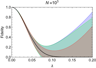
(a) (b)

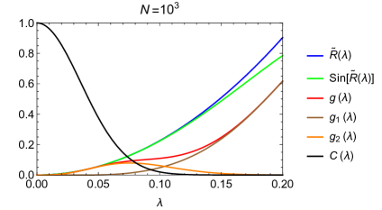
Figure 2: (Color online) Adiabatic fidelity $\mathcal{F}(\lambda)$ and generalized orthogonality catastrophe $\mathcal{C}(\lambda)$ described by the Hamiltonian (Bounds on quantum adiabaticity in driven many-body systems from generalized orthogonality catastrophe and quantum speed limit) with the parametrization (29) for $N=10^{3}$ sites. (a) Comparison between the old inequality (9) and the two improved inequalities (20) and (22). The black curve is for $\mathcal{C}(\lambda),$ which is, however, indistinguishable from $\mathcal{F}(\lambda)$ in the plot. The blue-shaded (resp., green- and red-shaded) region is the bound for $\mathcal{F}(\lambda)$ from $\widetilde{\mathcal{R}}(\lambda)$ (9) [resp., from $\sin\widetilde{\mathcal{R}}(\lambda)$ in Eq. (20) and from $g(\lambda)$ in Eq. (22)]. The red-shaded (resp., green-shaded) area is about 59% (resp., 95%) of the blue-shaded area. (b) Behavior of the functions $\widetilde{\mathcal{R}}(\lambda)$, $\sin\widetilde{\mathcal{R}}(\lambda)$, and $g(\lambda)=g^{\,}_{1}(\lambda)+g^{\,}_{2}(\lambda)$ (23) as a function of $\lambda.$ For comparison, $\mathcal{C}(\lambda)$ is also depicted. Refer to the main text for further explanation.

Setup of driven many-body systems.— Before considering a specific example in the next section, we follow Ref. Lychkovskiy et al. (2017) to specify a wide range of quantum systems that share general properties which the specific example possesses. The time-dependent Hamiltonian $H^{\,}_{\lambda}$ in which we are interested has a typical form,

$$H^{\,}_{\lambda}=H^{\,}_{0}+\lambda V,$$ (24)

where $H^{\,}_{0}$ is a time-independent Hamiltonian with the lowest energy eigenstate $|\Phi^{\,}_{0}\rangle$ and $V$ is a driving potential. We also assume that the driving rate $\Gamma=\partial^{\,}_{t}\lambda$ is a constant in $\lambda.$ It then follows that $\mathcal{R}(\lambda)$ [(8b)], the time integral of quantum uncertainty, reads

$$\mathcal{R}(\lambda) =\frac{\lambda^{2}}{2\Gamma}\delta V^{\,}_{N},\quad\delta V^{\,}_{N}\,\raisebox{0.85pt}{.}\raisebox{2.85pt}{.}\!\!=\,\sqrt{\langle\Phi^{\,}_{0}|V^{2}|\Phi^{\,}_{0}\rangle-\langle\Phi^{\,}_{0}|V|\Phi^{\,}_{0}\rangle^{2}}.$$ (25)

In other words, $\mathcal{R}(\lambda)$ is a monotonically increasing function in $\lambda^{2}$.

We further restrict ourselves to a broad class of time-dependent Hamiltonians whose generalized orthogonality catastrophe $\mathcal{C}(\lambda)$ (5) has the following simple exponentially decaying form when the system size, $N$, is large,

$$\ln\mathcal{C}(\lambda)=-C^{\,}_{N}\lambda^{2}+r(N,\lambda),\quad\lim_{N\to\infty}C^{\,}_{N}=\infty,$$ (26)

where the residual $r$ satisfies $\lim^{\,}_{N\to\infty}r(N,C^{-1/2}_{N})=0.$

Example: driven Rice-Mele model.— In order to demonstrate the validity of the improved inequalities, Eqs. (20) and (22), we consider the spinless Rice-Mele model on a half-filled one-dimensional bipartite lattice with the Hamiltonian Rice and Mele (1982); Nakajima et al. (2016)

$$H^{\,}_{\mathrm{RM}}= \sum^{N}_{j=1}\left[-(J+U)a^{{\dagger}}_{j}b^{\,}_{j}-(J-U)a^{{\dagger}}_{j}b^{\,}_{j+1}+\mathrm{h.c.}\right]$$

$$+\sum^{N}_{j=1}\Delta\left(a^{{\dagger}}_{j}a^{\,}_{j}-b^{{\dagger}}_{j}b^{\,}_{j}\right),$$ (27)

where $a^{\,}_{j}$ and $b^{\,}_{j}$ are the fermion annihilation operators on the $a$ and $b$ sublattices, respectively. Here, $N$ is the number of lattice sites. For the case of $J=U=\mathrm{const}$ and $\Delta=\lambda E^{\,}_{\mathrm{R}},$ where $\lambda=\Gamma t$ and $E^{\,}_{\mathrm{R}}$ is a recoil energy, it is shown in Ref. Lychkovskiy et al. (2017) that the exponent $C^{\,}_{N}$ defined in Eq. (26) and the quantum uncertainty $\delta V^{\,}_{N}$ defined in Eq. (25) read as follows:

$$C^{\,}_{N}=\frac{NE^{2}_{\mathrm{R}}}{16JU},\quad\delta V^{\,}_{N}=\sqrt{N}E^{\,}_{\mathrm{R}}.$$ (28)

Equation (28) with the chosen value of the parameters from Ref. Lychkovskiy et al. (2017),

$$(J,\;U,\;\Delta,\;\Gamma)=(0.4E^{\,}_{\mathrm{R}},\;0.4E^{\,}_{\mathrm{R}},\;\lambda E^{\,}_{\mathrm{R}},\;0.7E^{\,}_{\mathrm{R}}),$$ (29)

gives the following expressions for $\mathcal{C}(\lambda)$ (26) and $\mathcal{R}(\lambda)$ (25):

$$\mathcal{C}(\lambda)=e^{-N\lambda^{2}/(1.6)^{2}},\quad\mathcal{R}(\lambda)=\frac{\sqrt{N}\lambda^{2}}{1.4}.$$ (30)

Provided with Eq. (30), we present in Fig. 2 the comparison of bounds on the adiabatic fidelity $\mathcal{F}(\lambda)$ using the old inequality (9) and the two improved inequalities, Eqs. (20) and (22), for $N=10^{3}.$ Specifically, given the second improved inequality (22) and noting that $\mathcal{F}(\lambda)\in[0,1]$ by its definition, the following two-sided bound on the adiabatic fidelity $\mathcal{F}(\lambda)$ is obtained,

$$\max\left(\mathcal{C}(\lambda)-g(\lambda),\;0\right)\leq\mathcal{F}(\lambda)\leq\min\left(\mathcal{C}(\lambda)+g(\lambda),\;1\right).$$

Similar expressions apply to the old inequality (9) and the first improved inequality (20) with $g(\lambda)$ being replaced by $\widetilde{\mathcal{R}}(\lambda)$ and $\sin\widetilde{\mathcal{R}}(\lambda)$, respectively. Figure 2(a) shows that the second improved inequality (22) (as represented by the red-shaded region) greatly improves the estimate for $\mathcal{F}(\lambda)$ compared to the previous estimate (9) (as represented by the blue-shaded region). Figure 2(b) shows the behavior of functions $\widetilde{\mathcal{R}}(\lambda)$, $\sin\widetilde{\mathcal{R}}(\lambda)$, and $g(\lambda)=g^{\,}_{1}(\lambda)+g^{\,}_{2}(\lambda)$ (23) as a function of $\lambda.$ The function $g(\lambda)$ is dominated by $g^{\,}_{2}(\lambda)$ when $\lambda$ is small and is dominated by $g^{\,}_{1}(\lambda)$ when $\lambda$ is large. It can be understood from Eq. (23) that, for large $\lambda,$ $\mathcal{C}(\lambda)\approx 0,$ so that $g(\lambda)\approx g^{\,}_{1}(\lambda)\approx\sin^{2}\mathcal{R}(\lambda)$. Similarly, for small $\lambda$, $\sin(2\mathcal{R}(\lambda))\gg\sin^{2}\mathcal{R}(\lambda),$ so that $g(\lambda)\approx g^{\,}_{2}(\lambda).$

Clearly, the upper boundary of each shaded region in Fig. 2(a) is determined by $\mathcal{C}(\lambda)+\widetilde{\mathcal{R}}(\lambda)$ for the blue-shaded region, by $\mathcal{C}(\lambda)+\sin\widetilde{\mathcal{R}}(\lambda)$ for the green-shaded region, and by $\mathcal{C}(\lambda)+g(\lambda)$ for the red-shaded region. Observe from Fig. 2(b) that the function $\mathcal{C}(\lambda)$ is an exponentially decaying function in $\lambda,$ whereas the functions $\widetilde{\mathcal{R}}(\lambda)$, $\sin\widetilde{\mathcal{R}}(\lambda)$, and $g(\lambda)$ are monotonically increasing function in $\lambda$. As a result, the upper boundary of each shaded region in Fig. 2(a) has a valley when $\mathcal{C}(\lambda)$ is too small and then monotonically increases as $\lambda$ increases. Similarly, the bottom boundary of each shaded region in Fig. 2(a) is determined by $\mathcal{C}(\lambda)-\widetilde{\mathcal{R}}(\lambda)$, $\mathcal{C}(\lambda)-\sin\widetilde{\mathcal{R}}(\lambda)$, and $\mathcal{C}(\lambda)-g(\lambda),$ respectively. The bottom boundary is at zero when $\mathcal{C}(\lambda)\leq\left\{\widetilde{\mathcal{R}}(\lambda),\;\sin\widetilde{\mathcal{R}}(\lambda),\;g(\lambda)\right\}.$

To further investigate the effect of increasing system size on the bounds for the adiabatic fidelity $\mathcal{F}(\lambda)$, we plot in Fig. 3 the cases of $N=10^{4}$ and $N=10^{5}.$ For both cases, the green-shaded area is almost identical to the blue-shaded area, whereas the red-shaded area is about 34% (resp., 23%) of the blue-shaded area for $N=10^{4}$ (resp, for $N=10^{5}$). This indicates that the second improved inequality (22) is much stronger than the old inequality (9) as the number of lattice sites, $N$, increases. This fact can be understood by noticing that $\mathcal{C}(\lambda)$ (30), the generalized orthogonality catastrophe, decays quicker with increasing $N$; we are then forced to concentrate on the region of smaller $\lambda$. Consequently, it renders a smaller $g(\lambda)$, so that the bounds, $\mathcal{C}(\lambda)\pm g(\lambda)$, are tighter as $N$ increases.

Implication on adiabaticity breakdown.— This section discusses an implication from the second improved inequality (22) on the time scale for adiabaticity breakdown in generic driven many-body systems that possess the following asymptotic property,

$$\lim^{\,}_{N\to\infty}\frac{\delta V^{\,}_{N}}{C^{\,}_{N}}=0,$$ (31)

where $\delta V^{\,}_{N}$ is the quantum uncertainty of the driving potential (25) and $C^{\,}_{N}$ is the exponent of the generalized orthogonality catastrophe (26). As was pointed out in Ref. Lychkovskiy et al. (2017) using a general scaling argument, the asymptotic form (31) is obeyed by a wide range of Hamiltonians .

Now, combining the adiabaticity condition (3) and the bound on the adiabatic fidelity $\mathcal{F}(\lambda)$ from the second improved inequality (22) yields

$$1-\epsilon-\mathcal{C}(\lambda)\leq g(\lambda).$$ (32)

This inequality has to be satisfied if adiabaticity is established.

We follow the discussion of Ref. Lychkovskiy et al. (2017) to define the adiabatic mean free path $\lambda^{\,}_{*}$ as a solution to $\mathcal{F}(\lambda^{\,}_{*})=1/e.$ The leading asymptotic of $\lambda^{\,}_{*}$ reads

$$\lambda^{\,}_{*}=C^{-1/2}_{N}.$$ (33)

Observe that if the driving rate $\Gamma$ is independent of the system size $N$, then Eq. (31) indicates that $\mathcal{R}(\lambda=\lambda^{\,}_{*})$ (25) vanishes under the limit of large $N$,

$$\lim_{N\to\infty}\mathcal{R}(\lambda^{\,}_{*})=\frac{1}{2\Gamma}\lim_{N\to\infty}\frac{\delta V^{\,}_{N}}{C^{\,}_{N}}=0.$$ (34)

Consequently, under the same large $N$ limit, the asymptotic behavior (34) causes the function $g(\lambda)$ (23) to vanish when $\lambda\geq\lambda^{\,}_{*}$. If so, the inequality (32) with $\lambda=\lambda^{\,}_{*}$ reads $1-\epsilon-e^{-1}\leq 0$ as $N\to\infty.$ This means $\epsilon$ cannot be arbitrarily small; thus, adiabaticity fails.

In order to avoid the adiabaticity breakdown, one has to allow the driving rate $\Gamma$ to scale down with increasing system size $N$, $\Gamma=\Gamma^{\,}_{N}.$ Here, $\Gamma^{\,}_{N}$ is determined by setting $\lambda=\lambda^{\,}_{*}$ in the inequality (32) and approximating $\sin\mathcal{R}(\lambda^{\,}_{*})\approx\mathcal{R}(\lambda^{\,}_{*}).$ One finds

$$\Gamma^{\,}_{N}\leq\frac{1}{2}\frac{\delta V^{\,}_{N}}{C^{\,}_{N}}\frac{1}{1-\epsilon-e^{-1}}M,$$ (35)

where the multiplicative factor $M=e^{-1/2}\left(1-e^{-1}\right)^{1/2}+\left(1-e^{-1}-e^{-2}\right)^{1/2}\approx 1.187.$ Note that applying the same reasoning to the old inequality (9) delivers the multiplicative factor $M=1$ in Eq. (35), as was shown in Refs. Lychkovskiy et al. (2017, 2018). That is to say, compared to the old inequality (9), the improved inequality (22) does not affect the scaling form of the driving rate $\Gamma^{\,}_{N}$, but merely increases the multiplicative constant.

(a)

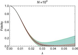
(b)

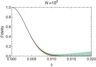
Figure 3: (Color online) Same as in Fig. 2 but with $N=10^{4}$ in panel (a) and $N=10^{5}$ in panel (b).

Summary and outlook.— In conclusion, we have derived two improved inequalities to bound the adiabatic fidelity using generalized orthogonality catastrophe and the quantum speed limit. These two inequalities are stronger than the previous result and are applicable to any quantum system. In particular, one of the two improved inequalities is nearly sharp when the system size is large.

In addition to quantum many-body systems, our method could also be applied to other fields in which bounds on adiabatic evolution are important, such as adiabatic quantum computation Farhi et al. (2000); Roland and Cerf (2002); Albash and Lidar (2018); Lychkovskiy (2018); Suzuki and Takahashi (2020) and adiabatic quantum control Rosenfeld and Zur (1996); Leghtas et al. (2011); Brif et al. (2014); Meister et al. (2014); Augier et al. (2018).

Acknowledgments. This work is part of the project Adiabatic Protocols in Extended Quantum Systems, Project No 680-91-130, which is funded by the Dutch Research Council (NWO).

S1 Derivation of the quantum speed limit (8)

This section provides an alternative derivation for the inequality of quantum speed limit (8). Our approach described below, inspired by Ref. Vaidman (1992), is pretty elementary as compared with the original proof given in Refs. Pfeifer (1993); Pfeifer and Fröhlich (1995) (see also the supplemental material of Ref. Lychkovskiy et al. (2017)).

We start by mentioning a simple formula. For any Hermitian operator $A$ and any quantum state $|\psi\rangle,$ there is a decomposition for $A|\psi\rangle$ taking the following form Aharonov and Vaidman (1990)

$$A|\psi\rangle=\langle A\rangle|\psi\rangle+\Delta A|\psi^{\,}_{\perp}\rangle,\qquad\langle\psi|\psi^{\,}_{\perp}\rangle=0,$$ (S1)

where $|\psi^{\,}_{\perp}\rangle$ is a vector orthogonal to $|\psi\rangle$, $\langle A\rangle=\langle\psi|A|\psi\rangle$ and $\Delta A=\sqrt{\langle A^{2}\rangle-\langle A\rangle^{2}}.$

We are given a time-dependent Hamiltonian $H^{\,}_{\lambda(t)}$ and the scaled time-dependent Schrödinger equation (2). The first step is to calculate the rate of the change of the fidelity $F(\Psi^{\,}_{\lambda},\Psi^{\,}_{0})$ (6) and use the scaled time-dependent Schrödinger equation (2) ($\hbar$ is restored in this section),

$$\frac{\partial}{\partial\lambda}F(\Psi^{\,}_{\lambda},\Psi^{\,}_{0})=\frac{\partial}{\partial\lambda}\Big{(}\langle\Psi^{\,}_{\lambda}|\Psi^{\,}_{0}\rangle\langle\Psi^{\,}_{0}|\Psi^{\,}_{\lambda}\rangle\Big{)}=2\Re\left(\left(\frac{\partial}{\partial\lambda}\langle\Psi^{\,}_{\lambda}|\right)|\Psi^{\,}_{0}\rangle\langle\Psi^{\,}_{0}|\Psi^{\,}_{\lambda}\rangle\right)=\frac{2}{\hbar\,\partial^{\,}_{t}\lambda}\Re\Big{(}\mathrm{i}\langle\Psi^{\,}_{\lambda}|H^{\,}_{\lambda}|\Psi^{\,}_{0}\rangle\langle\Psi^{\,}_{0}|\Psi^{\,}_{\lambda}\rangle\Big{)}.$$ (S2)

Next, the most crucial step is to decompose $H^{\,}_{\lambda}|\Psi^{\,}_{0}\rangle$ in Eq. (S2) using the formula (S1),

$$H^{\,}_{\lambda}|\Psi^{\,}_{0}\rangle=\langle H^{\,}_{\lambda}\rangle^{\,}_{0}|\Psi^{\,}_{0}\rangle+\Delta E^{\,}_{0}(\lambda)|\Psi^{\perp}_{0}\rangle,$$ (S3)

where $\langle H^{\,}_{\lambda}\rangle^{\,}_{0}=\langle\Psi^{\,}_{0}|H^{\,}_{\lambda}|\Psi^{\,}_{0}\rangle$ and $\Delta E^{\,}_{0}(\lambda)$ is defined in Eq. (8c). Substituting this decomposition into Eq. (S2) yields

$$\frac{\partial}{\partial\lambda}F(\Psi^{\,}_{\lambda},\Psi^{\,}_{0})=\frac{2\langle H^{\,}_{\lambda}\rangle^{\,}_{0}}{\hbar\,\partial^{\,}_{t}\lambda}\underbrace{\Re\Big{(}\mathrm{i}|\langle\Psi^{\,}_{\lambda}|\Psi^{\,}_{0}\rangle|^{2}\Big{)}}^{\,}_{=0}+\frac{2\Delta E^{\,}_{0}}{\hbar\,\partial^{\,}_{t}\lambda}\Re\Big{(}\mathrm{i}\langle\Psi^{\,}_{\lambda}|\Psi^{\perp}_{0}\rangle\langle\Psi^{\,}_{0}|\Psi^{\,}_{\lambda}\rangle\Big{)}.$$ (S4)

Upon taking absolute value for both sides and using the inequality $|\Re(z)|\leq|z|$ for $z\in\mathbb{C}$, the above equation reads

$$\left|\frac{\partial}{\partial\lambda}F(\Psi^{\,}_{\lambda},\Psi^{\,}_{0})\right|=\frac{2\Delta E^{\,}_{0}}{\hbar}\left|\frac{1}{\partial^{\,}_{t}\lambda}\Re\Big{(}\mathrm{i}\langle\Psi^{\,}_{\lambda}|\Psi^{\perp}_{0}\rangle\langle\Psi^{\,}_{0}|\Psi^{\,}_{\lambda}\rangle\Big{)}\right|\leq\frac{2\Delta E^{\,}_{0}}{\hbar|\partial^{\,}_{t}\lambda|}\left|\langle\Psi^{\,}_{\lambda}|\Psi^{\perp}_{0}\rangle\right|\left|\langle\Psi^{\,}_{0}|\Psi^{\,}_{\lambda}\rangle\right|.$$ (S5)

Now, recall that the physical state $|\Psi^{\,}_{\lambda}\rangle$ can be decomposed in terms of $|\Psi^{\,}_{0}\rangle$ and $|\Psi^{\perp}_{0}\rangle$ as in Eq. (10), the normalization condition of $|\Psi^{\,}_{\lambda}\rangle$ then implies $|\langle\Psi^{\,}_{\lambda}|\Psi^{\perp}_{0}\rangle|=\sqrt{1-|\langle\Psi^{\,}_{\lambda}|\Psi^{\,}_{0}\rangle|^{2}}=\sqrt{1-F(\Psi^{\,}_{\lambda},\Psi^{\,}_{0})}.$ Therefore, Eq. (S5) can be written as

$$\left|\frac{\partial}{\partial\lambda}F(\Psi^{\,}_{\lambda},\Psi^{\,}_{0})\right|\leq\frac{2\Delta E^{\,}_{0}}{\hbar|\partial^{\,}_{t}\lambda|}\sqrt{1-F(\Psi^{\,}_{\lambda},\Psi^{\,}_{0})}\sqrt{F(\Psi^{\,}_{\lambda},\Psi^{\,}_{0})}.$$ (S6)

After introducing the Bures angle (7), the above equation reads

$$\left|\frac{\pi}{2}\frac{\partial}{\partial\lambda}D(\Psi^{\,}_{\lambda},\Psi^{\,}_{0})\right|\leq\frac{\Delta E^{\,}_{0}}{\hbar|\partial^{\,}_{t}\lambda|}\qquad\Rightarrow\qquad-\frac{\Delta E^{\,}_{0}}{\hbar|\partial^{\,}_{t}\lambda|}\leq\frac{\pi}{2}\frac{\partial}{\partial\lambda}D(\Psi^{\,}_{\lambda},\Psi^{\,}_{0})\leq\frac{\Delta E^{\,}_{0}}{\hbar|\partial^{\,}_{t}\lambda|},$$ (S7)

which can be integrated over $\lambda$ to obtain (recall $D(\Psi^{\,}_{\lambda},\Psi^{\,}_{0})\geq 0$ by definition)

$$\frac{\pi}{2}D(\Psi^{\,}_{\lambda},\Psi^{\,}_{0})\leq\frac{1}{\hbar}\int^{\lambda}_{0}\frac{\mathrm{d}\lambda^{\prime}}{|\partial^{\,}_{t}\lambda^{\prime}|}\Delta E^{\,}_{0}(\lambda^{\prime}).$$ (S8)

Hence, the proof of Eq. (8) is complete.

Note that in Eq. (S2), if we instead apply the key formula (S1) to $\langle\Psi^{\,}_{\lambda}|H^{\,}_{\lambda}$, we shall obtain the following version of the quantum speed limit

$$\frac{\pi}{2}D(\Psi^{\,}_{\lambda},\Psi^{\,}_{0})\leq\frac{1}{\hbar}\int^{\lambda}_{0}\frac{\mathrm{d}\lambda^{\prime}}{|\partial^{\,}_{t}\lambda^{\prime}|}\Delta E(\lambda^{\prime}),$$ (S9)

where $\Delta E(\lambda)=\sqrt{\langle\Psi^{\,}_{\lambda}|H^{2}_{\lambda}|\Psi^{\,}_{\lambda}\rangle-\langle\Psi^{\,}_{\lambda}|H^{\,}_{\lambda}|\Psi^{\,}_{\lambda}\rangle^{2}}$ is the quantum uncertainty of $H^{\,}_{\lambda}$ with respect to $|\Psi^{\,}_{\lambda}\rangle.$ For a time-independent Hamiltonian, Eq. (S9) is identical to Eq. (S8). This type of quantum speed limit is known as Mandelstam-Tamm inequality in literature Mandelstam and Tamm (1945); Deffner and Campbell (2017).

S2 Direct proof of the inequality (19)

In this section, we want to prove the inequality (19) using an elementary method. In terms of the fidelity (6) and the Bures angle (7), the inequality (19) reads

$$\left|F\left(\Phi^{\,}_{\lambda},\Psi^{\,}_{\lambda}\right)-F\left(\Phi^{\,}_{\lambda},\Phi^{\,}_{0}\right)\right|\quad\leq\quad\sin\left(\frac{\pi}{2}D(\Psi^{\,}_{\lambda},\Psi^{\,}_{0})\right).$$ (S10)

Indeed, this inequality is an instance of the following lemma Rastegin (2002, 2003):

Lemma 1.

For each triplet $\{|\psi^{\,}_{1}\rangle,|\psi^{\,}_{2}\rangle,|\psi^{\,}_{3}\rangle\}$ of states, the following inequality holds:

$$\left|F\left(\psi^{\,}_{1},\psi^{\,}_{2}\right)-F\left(\psi^{\,}_{1},\psi^{\,}_{3}\right)\right|\leq\sin\left(\frac{\pi}{2}D(\psi^{\,}_{2},\psi^{\,}_{3})\right),$$ (S11)

where $F(.,.)$ is the fidelity (6) and $D(.,.)$ is the Bures angle (7).

Proof.

Apply the following triangle inequality

$$D(\psi^{\,}_{2},\psi^{\,}_{3})\leq D(\psi^{\,}_{1},\psi^{\,}_{2})+D(\psi^{\,}_{1},\psi^{\,}_{3}),$$ (S12)

and the trigonometric formula, $\cos^{2}x-\cos^{2}y=\sin(x+y)\sin(y-x)$, to the left side of Eq. (S11)

$$F\left(\psi^{\,}_{1},\psi^{\,}_{2}\right)-F\left(\psi^{\,}_{1},\psi^{\,}_{3}\right) =\cos^{2}\left(\frac{\pi}{2}D(\psi^{\,}_{1},\psi^{\,}_{2})\right)-\cos^{2}\left(\frac{\pi}{2}D(\psi^{\,}_{1},\psi^{\,}_{3})\right)$$

$$\leq\cos^{2}\left(\frac{\pi}{2}D(\psi^{\,}_{2},\psi^{\,}_{3})-\frac{\pi}{2}D(\psi^{\,}_{1},\psi^{\,}_{3})\right)-\cos^{2}\left(\frac{\pi}{2}D(\psi^{\,}_{1},\psi^{\,}_{3})\right)$$

$$=\sin\left(\frac{\pi}{2}D(\psi^{\,}_{2},\psi^{\,}_{3})\right)\sin\left(\pi D(\psi^{\,}_{1},\psi^{\,}_{3})-\frac{\pi}{2}D(\psi^{\,}_{2},\psi^{\,}_{3})\right)$$

$$\leq\sin\left(\frac{\pi}{2}D(\psi^{\,}_{2},\psi^{\,}_{3})\right).$$ (S13)

Exchange the role of $|\psi^{\,}_{2}\rangle$ and $|\psi^{\,}_{3}\rangle$ in Eq. (S13) yields

$$F\left(\psi^{\,}_{1},\psi^{\,}_{3}\right)-F\left(\psi^{\,}_{1},\psi^{\,}_{2}\right) =\cos^{2}\left(\frac{\pi}{2}D(\psi^{\,}_{1},\psi^{\,}_{3})\right)-\cos^{2}\left(\frac{\pi}{2}D(\psi^{\,}_{1},\psi^{\,}_{2})\right)$$

$$\leq\sin\left(\frac{\pi}{2}D(\psi^{\,}_{2},\psi^{\,}_{3})\right).$$ (S14)

Upon combing Eqs. (S13) and (S14), the proof of Eq. (S11) is therefore complete. ∎