Understanding the surface wave characteristics using 2D particle-in-cell simulation and deep neural network

Abstract

The characteristics of the surface waves along the interface between a plasma and a dielectric material have been investigated using kinetic Particle-In-Cell (PIC) simulations. A microwave source of GHz frequency has been used to trigger the surface wave in the system. The outcome indicates that the surface wave gets excited along the interface of plasma and the dielectric tube and appears as light and dark patterns in the electric field profiles. The dependency of radiation pressure on the dielectric permittivity and supplied input frequency has been investigated. Further, we assessed the capabilities of neural networks to predict the radiation pressure for a given system. The proposed Deep Neural Network model is aimed at developing accurate and efficient data-driven plasma surface wave devices.

I Introduction

Waves in the bounded plasma have gained considerable interest in the last few decades. While studying the interaction of an electromagnetic field with the plasma, along with bulk wave modes, it is also important to consider the wave mode concentrated at the surface.Such modes are known as surface waves. Such waves play a very crucial role in understanding plasma turbulence in the divertor of laboratory fusion deviceslee2021collisional , torus of fluidnovkoski2021experimental , plasma diagnostics, laser physicsluo2013laser , communication, atomic spectroscopyhubert1996atomic , high-density plasma generations, and even in plasma processing. Furthermore, in astrophysical plasma, surface wave energy transport has an important role in understanding the magnetosphere and solar corona problems gordon1983collisional ; shu1992volume ; roth2010surface ; buti1990solar . Steinolfson et al.steinolfson1986viscous found that at higher frequencies, the viscous damping of surface waves can cause the heating of the solar corona. Even in quantum plasma, surface wave study has made quite good imprints. To name a few, Lazar et al.lazar2007surface investigated the dispersion properties of the surface wave by incorporating the quantum statistical pressure as well as the quantum tunneling effects and observed that these effects make it easier for the electrostatic surface waves to propagate in plasma. Shahmansouri et al.shahmansouri2017exchange , investigated the influences of Coulomb interaction along with other quantum forces and the external magnetic field to understand the properties of ion-acoustic surface waves.

The surface wave is an electromagnetic wave localized at the surface, which propagates along with the interface of mediums having different permittivity. The name comes from the notion of carrying energy, mainly in the near interface region, and decays exponentially away from the interface. Such nature of a wave is also known as an evanescent wave. In plasma physics, the surface wave propagation takes place only if the dielectric permittivity of the medium is negative briggs:1970 . For cold plasma approximation, the permittivity is described as $\epsilon_{p}=1-\omega_{pe}^{2}/\omega^{2}$, where $\omega_{pe}$ is the plasma frequency and $\omega$ is the wave frequency. When such a medium with negative permittivity is surrounded by a dielectric of positive permittivity, $\epsilon_{d}$, the propagation takes place along the interface with frequency $\omega$ $\leq$ $\omega_{pe}/(1+\epsilon_{d})^{1/2},$ where $\epsilon_{d}$ is the relative permittivity of glassmoisan1975small . Upon satisfaction of the given condition, plasma can sustain the surface wave with an evanescent field on both the sideslandau1960 . Such nature of the wave aids in dumping the energy into the system, resulting in rapid ionization in the plasma medium. Plasma surface waves were first observed experimentally by Trivelpiece and Gould trivelpiece1959space using a cylindrical plasma column bounded by dielectric. After that, the surface wave has been investigated considering the interface separating the media of two different dielectricsjanaki1998surface ; Mishra_2018 ; cramer1996alfven ; ivanova1993radiophysics ; Mishra_void . For many early years, high-frequency discharges have been maintained between the metal electrodes or the resonant cavities. However, the method was very complex to maintain the discharge. Then a new way of plasma production was proposed that can reduce some complexity of already existing devices based on RF and microwave frequencies. The new method uses electromagnetic (EM) surface waves to sustain the dischargemoisan1975small . Eventually, the interest in such waves attracted researchers to use in sustaining plasma columns. Therefore, in the 1970s, a simple, compact, and well-organized device named surfatron was developed, which uses electromagnetic surface waves to generate plasma columns at microwave frequenciesmoisan1975small ; moisan1991plasma . It does not require any external magnetic field along the column (plasma) axis or other additional devices to sustain the plasma, like other devices. As the electrodes are not required for the wave excitation, the problem of gas contamination and the corrosion of the electrodes due to interaction with the plasma gets reduced. Apart from the ease of plasma sustainability, such systems have amazing applications in the field of communication technology as plasma antennas. A plasma antenna is the best alternative for a traditional metal antenna with re-configurable input capability. Several articles reported the theoretical and experimental investigation of the surface wave and its characteristicskaw1970 ; margot1993 ; Baruthram1993 ; lee1995 ; lee2000 in the context of its usage as antenna. However, there are still open questions regarding surface wave physics yet to be answered that would provide a new perspective about the field.ott:2008 ; omelchenko:2012

Besides the laboratory and industrial investigation, several authors have studied surface waves using different numerical simulation techniques. To begin with, Kousaka et al.kousaka2002numerical studied the propagation of electromagnetic waves along the plasma dielectric interface wave using the 2D finite difference time domain (FDTD) approximation. Igarashi et al.igarashi2004finite investigated the plasma surface wave using the finite element method. Kabouzi et al.kabouzi2007modeling used a self-consistent two-dimensional fluid-plasma model coupled with the Maxwell equations for surface wave sustained argon plasma discharge. Despite all these investigations described above, we believe that there is a significant gap in understanding regarding the kinetic properties of plasma in support of the surface wave propagation.

In the present work, we have investigated surface waves and their kinetic characteristics. There are various factors on which the surface wave propagation depends. Parameters like plasma density, source frequency, and surface material permittivity are a few of the important ones among those factors. Out of which, we have considered the source frequency and the material permittivity to study the surface wave characteristics. To quantify the impact of the aforementioned parameters, we have observed the radiation pressure pattern in the presence of surface waves. The work is performed using particle-in-cell (PIC) simulation birdsall1991plasma of an argon plasma with XOOPICverboncoeur1995object . The code uses the Monte Carlo collision algorithm vahedi1995monte to model collisions with neutrals in the system. The result presented in this work is believed to add new physical aspects of the surface wave sustained plasma column to aid future experimental investigations and innovations.

One of the unique aspects of the present work comes in the form of application of Deep Neural Network (DNN) to predict the radiation characteristics of a given system. Deep Learning is a sub-field of machine learning in Artificial intelligence (A.I.) that deals with algorithms inspired by biological neurons. It uses sophisticated mathematical modeling to process data in complex ways. DNN consists of neural networks that have an input layer, an output layer, and at least one hidden layer in between. In the neural network, the input layer is the first layer that accepts the external information or data and passes it into the input layer’s units. The output layer is the last layer of the neural network that produces outputs for the model. It provides the outcome or prediction of the data fed into the input layer. Hidden layers are the intermediate layer between the input and output layers. There can be either one or more hidden layers in a network. Being a combination of neural network and machine learning, DNN provides a perfect tool to leverage deep learning for all machine learning tasks and expect better performance with surplus data availability. With the advent of cost-effective computing power and data storage, deep learning has been embraced in every digital corner of our everyday life. However, there is a big gap in research-based physical models as of now. The usability of DNN is unlimited if a user can train such a model with physics-based parameters. In recent studies, it has shown promising outcomes in terms of accurate prediction of physical quantitiescheng2021deep ; raissi2019physics ; lagaris1998artificial ; adhikari:2021 . The need for such a model appears due to computationally expensive kinetic codes such as PIC. For example, a typical run of XOOPIC with the presented system configuration takes 10-12 hours (wall-time) depending on the number of particles used. In order to reduce statistical noise, that number can ever go up to 36-40 hours. Now, this is why a consolidated artificially trained model is essential such that prediction of radiation data becomes numerically cheap. In the present work, we have built a DNN model comprising a complex neural network of several layers to predict estimated radiation data for a given plasma system. Additionally, we have made it open-source, such that people can contribute their data to improve the accuracy of their model and experimental facilities.
The paper has been organized as follows. Section II presents the simulation model for the study, followed by results and discussion of the work in section III. Section IV describes the implementation and usage of the Deep Neural Network (DNN) in the present work. Lastly, we conclude the work in section V.

II Simulation method and modeling

In the present work, the interaction of plasma with an electromagnetic field inside a dielectric tube has been studied using a Particle-in-Cell simulation code (XOOPICverboncoeur1995object ). It is an X-Windows version of OOPIC, which is a two-dimensional relativistic electromagnetic object-oriented particle-in-cell code written in the C++ programming language. . The PIC method is preferred over others to better understand the non-linear properties of plasma and kinetic behavior. It models a plasma system consisting of a large number of superparticles (having the same charge to mass ratio as the real plasma particles) distributed in a spatial domain. The charge and current densities are calculated using the superparticle’s position and velocity data in a spatial domain. Maxwell’s equations are solved at each time step for discrete mesh points, and particles are moved by the resulting forces calculated on the particles. A detailed description of the algorithm of XOOPIC code can be found in a paper written by Verboncoeur et al. verboncoeur1995object . It has features of modeling two spatial dimensions in both Cartesian (x,y) and cylindrical(r,z) geometry, including all three velocity components. The applicability of this code ranges from plasma discharges, such as glow and RF discharges, to microwave-beam devices. The code can handle an arbitrary number of species and includes Monte Carlo Collision (MCC) algorithms for modeling intra-species collisions of charged particles as well as collisions with the neutral background gas.

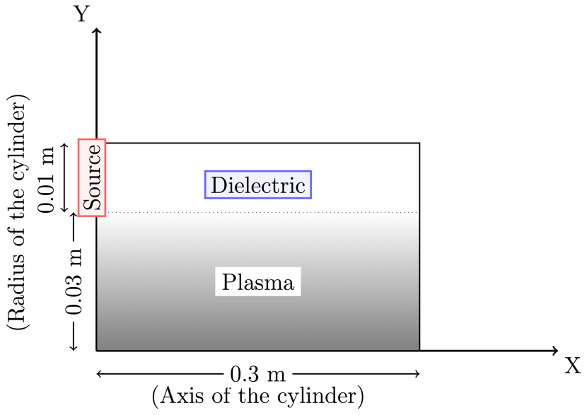
Figure 1: Schematic of our simulation model. Length of the tube in x, and y direction are 0.3 m and 0.03 m respectively. The thickness of the dielectric tube is 0.01 m. Source of microwave frequency 2.45 GHz is placed at the left top of portion of the model. The left and right boundary of the system is considered to be absorbing.

The model is developed considering the symmetric half of the cylinder on Cartesian geometry. The schematic of our model is given in fig. 1. The length of the cylinder is considered to be $0.3$ m in the x-direction and $0.03$ m in the y-direction. The top boundary is a dielectric material with a thickness $0.01$ m. The left and right boundaries of the plasma system are considered to be nearly perfect conductors (for the fields) and to absorb the incident particles. Particles (electrons and Argon ions) are loaded uniformly throughout the domain from Maxwellian distributions with respective temperatures $T_{e}$ and $T_{i}$ (see table 1). The plasma density is sustained by ionization via collision with the constant background neutrals (pressure of $0.1$ Torr). However, the ionization of the second and higher-order argon atoms is neglected. A source of microwave frequency ($f_{source}$) at $2.45$ GHz is added using a wave port (at the left top portion of the model). The dielectric constant ($\epsilon_{r}$) of the surrounding material and the source frequency ($f_{source}$) are continuously varied to quantify the effects on radiation profile. For the baseline simulation, we have set $f_{source}$ at $2.45$ GHz and $\epsilon_{r}$ at $5$.

To maintain the stability of the numerical method, step size and grid size has been chosen carefully, satisfying the Courant condition de2013courant . The spatial grid is composed of 2048 ($Nx\times Ny$) cells of cell size $0.00468\times 0.00125$ m, which ensures that Debye length is resolved. On average, $39$ computational particles (super-particle) per cell are loaded, resulting in adequate resolution for the field quantities with minimum statistical noise. As mentioned, a time step of $10^{-12}~{}s$ is chosen to meet Courant criteria, ensuring electrons (fastest particle) never cross an entire spatial cell in one single time step. For each case, the simulation was run for $2\times 10^{6}$ timesteps, which translates into $2~{}\mu s$. In our modeling approach, we load a uniform density at the beginning in a similar fashion as others cooperberg1998series ; Matsumoto:M96/87 and run the simulation long enough to make sure the loss of particles at the walls and generation of particles due to charge-neutral collision is balanced. Each case was run to reach a quasi-stationary state and terminated when there were no significant changes in the plasma density profiles.

As we mentioned in the introduction, a typical run of XOOPIC can take 10-12 hours (wall-time) or may be even 36-40 hours based on grid resolution and statistical weight. We made a moderate choice of 20 hours per run for 1024 parametric variations. It approximately took 42 days using HPC (parallel and sequential).

Parameter	Value
Initial Plasma density ($N_{e,i}$)	$\sim 10^{14}~{}m^{-3}$
Final Plasma density ($N_{e,i}$)	$\sim 1.5\times 10^{16}~{}m^{-3}$ (baseline)
Electron temperature ($T_{e}$)	2 eV
Ion temperature ($T_{i}$)	0.03 eV
Debye length ($\lambda_{d}$)	$0.001$ m
Number of cells ($N_{x}$, $N_{y}$)	64, 32
Time step ($\delta t$)	$10^{-12}$ s
Spatial Grid size ($\delta x$, $\delta y$)	$0.00468$ m, $0.00125$ m
System length ($L_{x}$, $L_{y}$)	0.3 m, 0.04 m
No. of particles	102400 (baseline)
Neutral Gas	Argon (Ar)
Pressure	0.1 Torr

Table 1: Simulation Parameters.

III Results and discussions

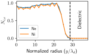
Figure 2: (a) Axial electric field and (b) density profiles along the radial direction in across the plasma and the dielectric medium. The black dotted line represents the interface of the plasma and the dielectric material. The frequency and the dielectric constants are considered to be $2.45$ GHz and 5 respectively. The axial electric field normalized by its maximum value (maximum electric field  $1.5\times 10^{4}$ V/m) and the density is normalized by the bulk plasma density $1.5\times 10^{16}~{}m^{-3}$. The radial length is normalized by the electron Debye length ($\lambda_{d}$) for both figures.

The physical properties of the surface wave have been investigated using the parameters given in table 1. Under the application of a microwave source, the interaction of the electromagnetic field with the plasma leads to the localization of surface charge near the interface region (charge bunching). The presence of surface charge causes the maximum electric field intensity in the region and the intensity decreases as we move away from the interface region (in the radial direction). Such behavior is known as an evanescent nature. Existing literature on plasma surface wave indicates that the evanescent nature is one of the assurances for the surface wave to exist. Figure 2 describes the spatial profile of the normalized electric field ($E_{x}$) and the densities along the radial direction (y-direction) for the baseline simulation. Here, the electric field has been normalized with its maximum value (maximum electric field  $1.5\times 10^{4}$ V/m) and the system radius (y) with electron Debye length. For the densities, bulk plasma density is taken as reference for normalization. The frequency and the dielectric constants for this figure have been considered $2.45$ GHz and $5$, respectively. It can be observed from the fig. 2 that near the dielectric surface, the field intensity is maximum and then decays in the radial direction, which points toward the existence of a surface wave. The general idea of surface wave study is based on the epitome of reality that only surface involved is the interface between two mediums. The surrounding vessel are the artifact of a more practical approach. The general approach of surface wave study is to neglect the effect of the plasma sheath. The argument for such consideration is the sheath scale length, $\lambda_{De}$, which is much less than the typical scale length (depth of penetration) of the surface wavecooperberg1998surface ; cooperberg1998series ; moisan1982properties ; lee2007kinetic ; lee2010kinetic . However, one can find such dispersion including the effect of sheath in the work by Cooperberg et al. cooperberg1998electron ; cooperberg1998nonuniform . For our case, we have also observed the existence of sheath near the interface region as shown in fig. 2(b).

The basic idea of surface wave generation in such systems is based on superposition of oppositely directed traveling waves from two different regions near the interface. Such superposition produces standing wave in which the plasma oscillates with certain frequency known as surface wave frequencytrivelpiece1959space . In fig. 3, we observe the normalized axial profile of the electric field, $E_{x}(x,y)$, normalized with its maximum value. The presence of positive and negative charge separated regions confirms the existence of standing waves in that region (shown as bright and dark patches in fig. 3). The plasma particles get trapped and oscillate with surface wave frequency. There is various literature also which supports our theory of surface wavezhelyazkov1978stimulated ; trivelpiece1959space ; cooperberg1998series . The color bar in the figures represents the intensity of the electric field denoted by $\zeta$.

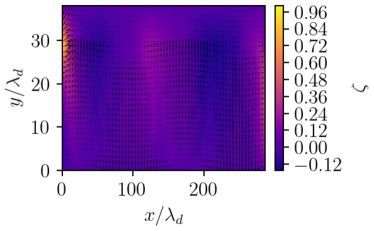
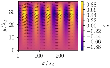
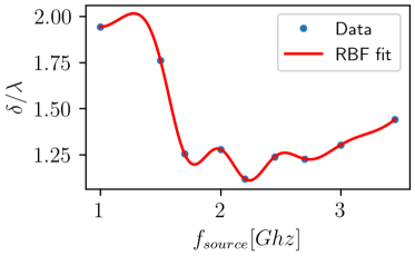
Figure 3: Profile of axial electric field intensity near the interface region for different frequency values. (a)Frequency - $1.7$ GHz (maximum electric field intensity  $3.6\times 10^{3}~{}V/m$), (b)Frequency - $2.45$ GHz (maximum electric field intensity  $6.4\times 10^{3}~{}V/m$), (c) Frequency - $3.45$ GHz (maximum electric field intensity  $1\times 10^{5}~{}V/m$). The colorbar in the figures represents the ratio of electric field intensity to its maximum value denoted by $\zeta$, (d) Pattern of the charge bunching width depending on the different frequency values using radial fit. $\delta$ in the figure represents the difference of the space charge width. The normalization of this parameter has been done by the wavelength of the wave $\lambda$.

The other observation from this field intensity profile is, at a frequency below the $2.45$ GHz frequency, the present model does not observe any charge bunching near the interface region (shown in fig. 3(a)). The reason might be the low energy input source, which might not be strong enough to increase the plasma density in order to excite the surface wave. The increasing frequency enhances the collision between the plasma particles and neutrals, exceeding the critical density. It causes the bunching of the surface charge near the interface leading to the excitation of surface wave propagation. However, for further increase in input frequency, we have also observed a decrease in the charge bunching width. Using the Radial Basis Function (RBF), fit for the data , fig. 3(d), shows the trend of charge-width variation depending on the frequency value. RBF method has been used for fitting as this method provides an excellent interpolant for high dimensional data sets of poorly distributed data points. In the figure $\delta$ represents the difference of the charge width. The normalization of this parameter has been done by the wavelength of the injected wave, $\lambda$.

Typically, glass is used as dielectric material to study surface wave propagation in plasma experiments. However, we perform a much generalized and detailed numerical study by considering the different permittivity values. The dependency of field intensity on the surrounding permittivity materials has been shown in fig. 4. Increasing material permittivity increases the conductivity, and the charge separation width decreases. Also the wave energy is concentrated mainly near the interface region. Moreover, increasing the dielectric value of the material makes the surface behave very differently, eventually the wave patterns get destroyed (shown in fig. 4(c)). In fig. 4(d), the trend of charge bunching width variation is shown depending on the permittivity value using the RBF fit.

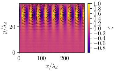
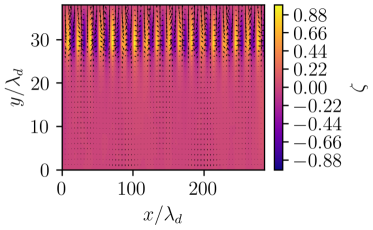
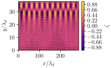
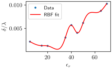
Figure 4: Profile of axial electric field intensity near the interface region for different permittivity variations.(a) permittivity - 20 (maximum electric field intensity  $1.6\times 10^{4}~{}V/m$), (b) permittivity - 50 (maximum electric field intensity  $7.2\times 10^{3}~{}V/m$), (c) permittivity - 100.(maximum electric field intensity  $1\times 10^{4}~{}V/m$). The colorbar in the figures represents the ratio of electric field intensity to its maximum value denoted by $\zeta$. (d) Pattern of the charge bunching width depending on the different permittivity values using radial fit. $\delta$ in the figure represents the difference of the charge width. The normalization of this parameter has been done by the wavelength of the wave $\lambda$.

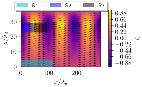
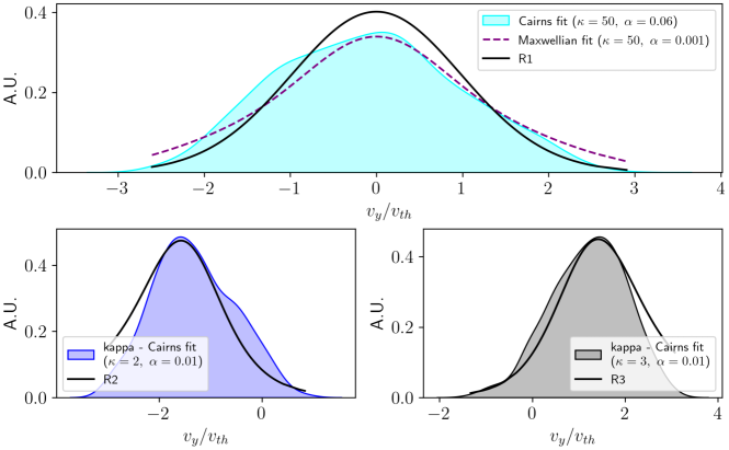
Figure 5: (a) Axial electric field intensity with highlighted areas used for velocity reconstruction. (b) Radial velocity distributions ($f(v_{y})$) of the electrons for different regions. The cyan profile represents the particle distribution in bulk region of the plasma i.e., R1 (0.0 - 114.2), The blue profile represents the particle distribution with left polarity, R2 (0.0 - 44.7) and black represents the distribution with right polarity, R3 (47.5 - 88.5). A.U is the arbitrary unit and $v_{th}$ is the thermal velocity of electrons. The bracketed numbers corresponding to each region are presented in normalized length scale ($\lambda_{d}$).

The velocity distribution of the electrons has been studied to understand their energy dynamics throughout the system (fig. 5b). The reconstruction of the velocity distribution is performed from the phase space at three different regions (see fig. 5a). Region R1 (0.0 - 114.1 $\lambda_{d}$) represents the bulk region of the system away from the interface. Regions R2 (0.0 - 44.7 $\lambda_{d}$) and R3 (47.5 - 88.5 $\lambda_{d}$) correspond to the different charge bunching regions with opposite polarity near the interface. Since we are interested in localized sampling, we also took a range in the radial direction for each axial range. For region R1, the radial range was taken as (0.0 - 4.7 $\lambda_{d}$), whereas for regions R2 and R3 (23.0 - 28.5 $\lambda_{d}$). To have a one-to-one correspondence, one should refer to the yellow and blue region in the electric field intensity profile (fig. 3b) for regions R2 and R3. Yellow and blue represent the localized positive and negative space charge regions, respectively.

To understand the distribution of particles in the presence of reverse-polarity structure, Cairns et al.cairns1995electrostatic introduced a particular non-thermal distribution known as Cairn’s distribution. Due to the evanescent nature of the surface wave field the magnitude of the field is higher near the interface region. Therefore, the particles gains more energy in that region compared to the bulk. The effect can be observed in the velocity distribution of the electrons in region 2 and region 3. The distribution obtained here is non-Maxwellian showing the high energy tail. Such deviation from Maxwellian distribution mostly occurs when the collisions between the high-energy particles and neutral particles are infrequent compared to the low energetic particles. The underlying reason for such occurrence is the mean free path of the higher energetic particles, which is proportional to $v^{4}$, where $v$ is the velocity of the particlesbara2014combined ; aman2020revisiting ; hadi2019kinetic . The quadratic factor comes from the Fokker-Planck theory, where the slowing downtime, $\tau_{s}\sim v^{3}$. The mean free path ($\lambda_{mfp}$) can be expressed as a product of particle velocity and slowing downtime, $v\tau_{s}$. Therefore, the mean free path bears the quadratic term. The detailed derivation is available in R. S. Marshall, and P. M. Bellan’s work marshall2019acceleration in addition to textbookskrallbook ; bellan2008fundamentals . Particles having such mean free path does not relax to a Maxwellian distribution state and shows the deviated distribution. Hence, the best fit for the profile naturally suits a Kappa-Cairns distribution. Such Kappa-Cairns distribution is usually found due to the presence of highly energetic non-thermal electrons and the co-existence of both the positive and negative potential. This might explain the reason behind the particles with the shifted Kappa-Cairns distribution near the interface region. The different polarity of the field defines the cause for the acceleration of the particles in different directions.

The Kappa-Cairns distribution:

$$f_{e}\left(\mathbf{v};v_{\mathrm{th}},\kappa,\alpha\right)=A_{\kappa,\alpha}\left(1+\alpha\frac{v^{4}}{v_{\mathrm{th}}^{4}}\right)\times\left(1+\frac{v^{2}}{2\left(\kappa-\frac{D}{2}\right)v_{\mathrm{th}}^{2}}\right)^{-(\kappa+1)},$$ (1)

where,

$$A_{\kappa,\alpha}=\frac{\Gamma(\kappa+1)/\Gamma\left(\kappa+\frac{2-D}{2}\right)}{\left(2\pi v_{\mathrm{th}}^{2}\left(\kappa-\frac{D}{2}\right)\right)^{\frac{D}{2}}\left[1+D(D+2)\alpha\frac{\kappa-\frac{D}{2}}{\kappa-\frac{D+2}{2}}\right]},~{}\kappa>\frac{D}{2}+1,$$

$v$ is the electron velocity (simulation data), $D=1,2,3$ for 1D, 2D, and 3D systems, $\kappa$ and $\alpha$ are the spectral indices of the distribution function, $v_{th}=\sqrt{\frac{kT_{e}}{m_{e}}}$ is the thermal velocity for the electrons.

For shifted Kappa-Cairns distribution,

$$f_{e}^{shift}\left(\mathbf{v};v_{\mathrm{th}},\kappa,\alpha\right)=A_{\kappa,\alpha}\left(1+\alpha\frac{v^{4}}{v_{\mathrm{th}}^{4}}\right)\times\left(1+\frac{(v-v_{shift})^{2}}{2\left(\kappa-\frac{D}{2}\right)v_{\mathrm{th}}^{2}}\right)^{-(\kappa+1)},$$ (2)

In region 1, further away from the surface, the electron distribution starts to take the form of a Maxwellian. The slight deformity in the distribution might be due to the high energetic particles (produced through the interaction of plasma with electromagnetic wave) near the interface can possibly move towards the bulk region. The bulk plasma is quite close to the interface (0.03 m away, as shown in the model). We believe this could be one of the reasons for obtaining the Cairns distribution or shifted Maxwellian distribution in the bulk region. If the system size in the radial direction is taken large, particles may lose their energy interacting with the background. In such case we may end up with a perfect Maxwellian distribution. However, it is needless to say such small change does not alter the dynamics of the system. Therefore, we did not modify the system radius as it would increase the computational hours without significant improvement of the results. Although, we could not confirm the reason behind the resemblance of the distribution towards Cairns fit in the present context. The above finding might be the scope for future works.

In fig. 6, the spatial profile of the time-averaged power density is deposited into the electrons that causes the heating of the plasma near the interface. In the earlier investigation, it has been found that at high-pressure range, ohmic heating is the dominant heating mechanism in RF plasma systemcooperberg1998series . Such a heating mechanism is responsible for the visible glow near the interface region. The appearance of such glow occurs due to the short mean free path for inelastic scattering, which causes the fast-moving electrons to lose energy quickly while moving away from the interface. The profile of electron heating shows the wavelike structure due to the presence of strong resonant surface wave fields. This makes the non-uniform heating profile of plasma in x-direction (axial direction). The strong field causes the generation of hot electron population in that region. Permittivity values in figures (a) and (b) have been used as 5 and 20, respectively, and the source frequency is considered to be $2.45$ GHz. The value of the power density is represented by $J$ and is normalized by its maximum value and denoted by $\hat{J}$.

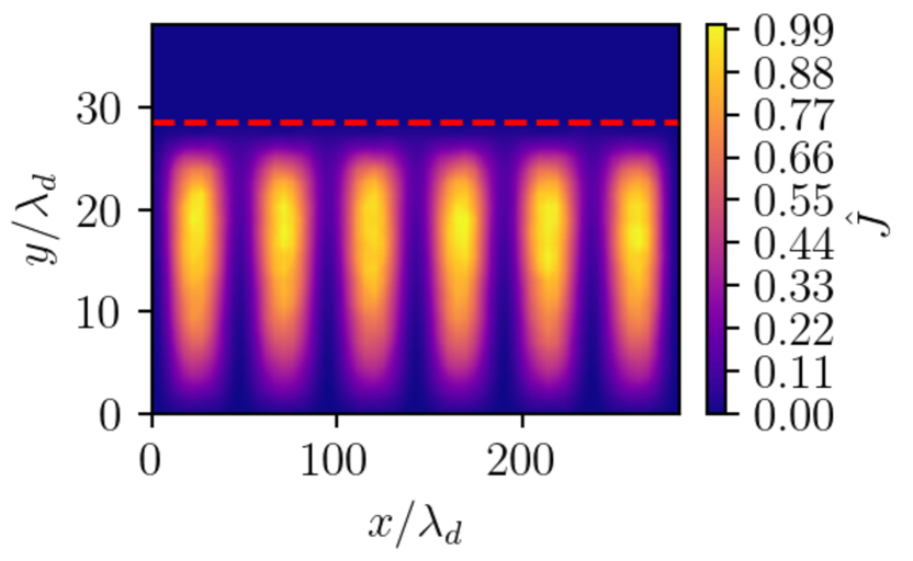
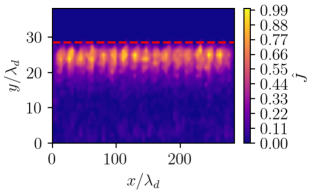
Figure 6: Spatial profile of the power deposited in the plasma by the field. The red dashed line represents the interface separating the plasma and the dielectric. The value of the power density is represented by $J$ and is normalized by its maximum value and denoted by $\hat{J}$. (a) Source frequency - $2.45$ GHz, and permittivity - 5 (maximum value of power deposited is $~{}10^{4}~{}\mathrm{Wm}^{-2}$), (b) Source frequency - $2.45$ GHz and permittivity - 20, (maximum value of power deposited is $\sim 10^{3}~{}\mathrm{Wm}^{-2}$).

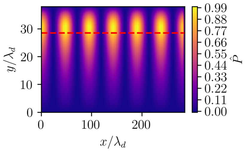
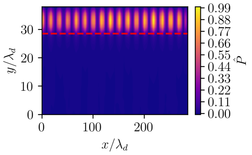
Figure 7: Radiation pressure in y-direction. The red dashed line represents the interface separating the plasma and the dielectric. The value of the radiation pressure is represented by P and is normalized by its maximum value and denoted by $\hat{P}$. (a) radiation profile for source frequency $2.45$ GHz and permittivity value 5 (maximum radiation pressure $~{}10^{-4}~{}\mathrm{Nm}^{-2}$), (b) radiation profile for source frequency $2.45$ GHz and permittivity value 20 (maximum radiation pressure $~{}10^{-5}~{}\mathrm{Nm}^{-2}$).

The radiation profile of the system is given in fig. 7. The presence of localized electric and magnetic fields near the interface region shows strong peaks in that region. As the radiation pressure represents the energy loss in the medium, the value of relative permittivity decides how the radiation will behave in the system. In fig. 7(a), it can be observed that for low permittivity (for the baseline parameters), the waves in the plasma system loose their energy as they move towards the bulk region (diminishing radiation pattern). However, for higher permittivity ($\epsilon_{r}$ = 20 and $f_{source}$ = $2.45$ GHz) the dielectric material contains the injected wave and absorbs all the emitted radiation into the dielectric medium (shown in fig. 7(b)). We have observed the same trend for even higher permittivity values. The take away is there is a threshold for permittivity to be used as a surrounding material for surface wave instruments.

IV Deep Neural Network Model

In this section, we have built a Deep Neural Network (DNN) model using Particle-in-Cell simulation data sets to predict the estimated radiation data based on the system parameters of any given system.

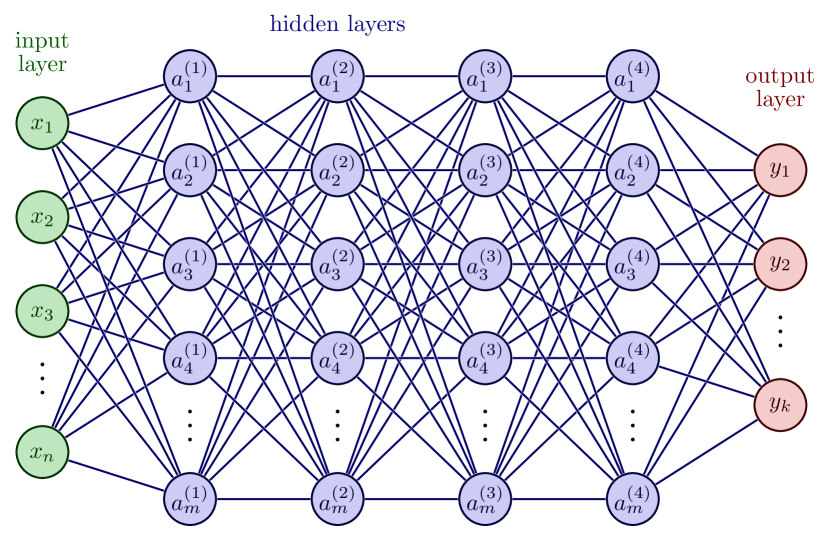
Figure 8: Schematic of the DNN model. A derivative illustration of “Izaak Neutelings, TikZ.net; licensed under a Creative Commons Attribution-ShareAlike 4.0 International License.”

Figure fig. 8 represents the schematic of a standard DNN model for such a purpose. The input layer ($x_{i}$, $i=0,1,2,...,n$, where $i$ = no. of dependent parameters or degrees of freedom) has been constructed from critical system parameters like input source frequency, dielectric permittivity of the surface material. The hidden layers ($a_{l}^{(j)}$, where, $j=1,2,..,4$, and $l=1,2,..,m$) have been developed using standard TensorFlow models from Keras (e.g. relu, selu, elu etc.). The number of hidden layers has been kept limited to 4 for the present work. The output layer ($y_{o}$, where, $o=1,2,..,k$) will give us the spatial dependence of radiation pattern for a specific system input. For the present case, we have considered $k=1$. After several tests, we finalized our multilayer perceptrons (MLPsgardner1998artificial ; rumelhart1985learning ) with four hidden layers each consisting 100 neurons (nodes). fig. 9 has been introduced to visualize neural networks’ architecture and understand how the different layers are connected with different neurons. For the MLP, we have used two specific element-wise nonlinear functions called layer activation functions from Keraskerasactivation , Rectified Linear Unit (RELU), and Scaled Exponential Linear Unit (SELU). A variant of the stochastic gradient descent algorithm referred to as ADAptive Moment estimation or ADAM has been used for the training runs. One of the important reasons for training an MLP is to determine the weight and biases using training data for the activation functions. The weights and biases depend on the choice of the loss function. For the present model, we have opted the standard choice for regression problems, the Mean Squared Error (MSE). In fig. 10 the training and validation loss for the model is plotted as a function of the number of epochs. We have used 25% of the training data as a validation set and considered early stopping to avoid over-fitting.

To test our DNN network, we randomized the input data set keeping the output data tethered and created two unique data set comprised of 1000 data points. A comparison between the simulated data and the ML predicted data is shown on fig. 11. The predicted values are found to lie within $2\sigma$ limit.

The DNN source code has been made available under MIT License. User can find the relevant details by visiting Zenodo or GitHubMishra_deepRadiation_2022 (doi:10.5281/zenodo.6300930).

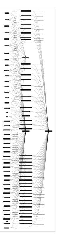
Figure 9: A visual representation of our DNN model. (Click to zoom)

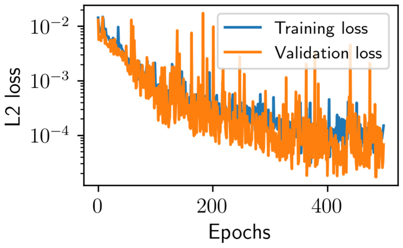
Figure 10: Training and validation loss as a function of the number of epochs for the DNN model.

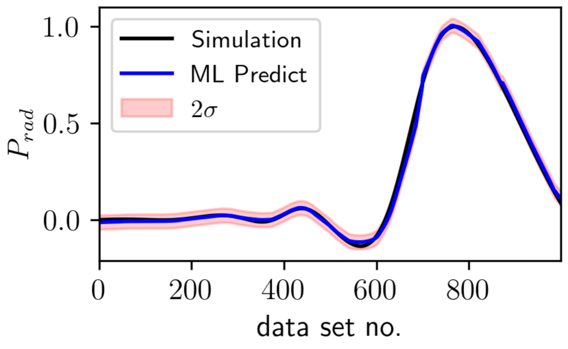
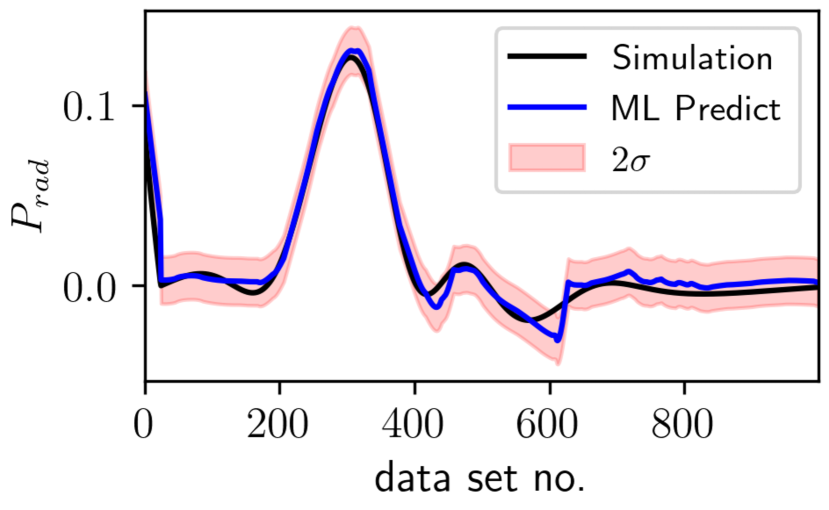
Figure 11: Normalized radiation pressure predicted by the network for different sets of known input data (source frequency, dielectric permittivity) along with true data from simulation. Radiation pressure is normalized with maximum value available in the training data set. Top (a) and bottom (b) panels represent the network performance of two randomly selected series of data sets.

V Conclusions

Our simulation model confirms the existence of the surface wave by the evanescent nature of the field. The principal focus of the present study was to examine the properties of the surface wave for different source frequency and permittivity values. It has been observed that at particular cutoff frequency, the model supports the charge bunching indicating the existence of surface wave. Below that frequency the system does not show any bunching or surface wave propagation. We have also noticed, with increasing frequency the bunching width ($\delta$) starts to decrease . The material permittivity has also a significant effect on the charge separation. Increasing permittivity for the surrounding material decreases the charge separation width. The presence of surface wave has some adverse effects on the electron dynamics. The energy of the electrons throughout the system has been studied using the reconstructed velocity distribution. Near the interface the electrons seem to follow the Kappa-Cairns distribution, whereas, in the bulk region of plasma (near to origin), they approach the Maxwellian distribution. However, the distribution was slightly deviated from Maxwellian, which we suspect due to small influx of higher energy particles towards the bulk region. The electron heating present in the system is very much different from the usual discharge process as it can be controlled by the supplied input frequency and the permittivity value. The presence of the surface wave field is responsible for the hot electron population in the near interface region. The parameters considered for the study also seem to affect the radiation pressure which constitutes the energy loss in the system. From the observations, we can suggest that the large permittivity material might not be a good choice for the surface wave study. The above observation demonstrate that the sustainment of the surface wave is configurable, hence can be controlled by physical parameters.

Deep Neural Network (DNN) has been introduced as a possible alternative to running PIC simulations for estimation of radiation pressure. For the present scenario, the degrees of freedom (DNN model) is two (source frequency and permittivity). The ideal would have been to include the length and radius of the system, which would increase the total number of runs multi-fold. With a moderate statistical noise for 1024 parametric variations ($\sim$ 20 hours per run), it took almost 42 days using HPC (parallel and sequential). Keeping the run-time and computational budget in mind, we tried to keep the total number of inputs (degree of freedom) limited to the case. In our opinion, the present way of using the PIC simulation as the data acquisition method for constructing a DNN model might be an impractical approach due to its computational cost. However, the open-source nature of the code and flexible input parameter space can allow people to expand the model to build on top of the existing datasets without rerunning the entire parameter space.

DATA AVAILABILITY

The data that support the findings of this study are available from the corresponding author upon reasonable request.

References

References

- [1] Myoung-Jae Lee and Young-Dae Jung. Collisional damping of the surface ion-acoustic mode in semi-bounded plasmas. Plasma Physics and Controlled Fusion, 63(11):115011, 2021.
- [2] Filip Novkoski, Eric Falcon, and Chi-Tuong Pham. Experimental dispersion relation of surface waves along a torus of fluid. Physical Review Letters, 127(14):144504, 2021.
- [3] Daobin Luo, Penghui Qi, Runcai Miao, and Jianke Liu. Laser diffraction from a liquid surface wave at low frequency. Laser Physics, 23(6):065701, 2013.
- [4] J Hubert, S Bordeleau, KC Tran, S Michaud, B Milette, R Sing, J Jalbert, D Boudreau, M Moisan, and J Margot. Atomic spectroscopy with surface wave plasmas. Fresenius’ journal of analytical chemistry, 355(5):494–500, 1996.
- [5] BE Gordon and JV Hollweg. Collisional damping of surface waves in the solar corona. The Astrophysical Journal, 266:373–382, 1983.
- [6] Frank Shu. Volume 2: Gas Dynamics. University Science Books, 1992.
- [7] M Roth, M Franz, N Bello Gonzalez, V Martinez Pillet, JA Bonet, A Gandorfer, P Barthol, SK Solanki, T Berkefeld, W Schmidt, et al. Surface waves in solar granulation observed with sunrise. The Astrophysical Journal Letters, 723(2):L175, 2010.
- [8] B Buti. Solar and planetary plasma physics. In SOLAR AND PlANETARY PlASMA PHYSICS: Invited Reviews of the 1989 PLasma Physics College, pages 1–242. World Scientific, 1990.
- [9] RS Steinolfson, ER Priest, Stefaan Poedts, L Nocera, and Marcel Goossens. Viscous normal modes on coronal inhomogeneities and their role as a heating mechanism. The Astrophysical Journal, 304:526–531, 1986.
- [10] M Lazar, PK Shukla, and A Smolyakov. Surface waves on a quantum plasma half-space. Physics of Plasmas, 14(12):124501, 2007.
- [11] M Shahmansouri, B Farokhi, and R Aboltaman. Exchange interaction effects on low frequency surface waves in a quantum plasma slab. Physics of Plasmas, 24(5):054505, 2017.
- [12] RJ Briggs, JD Daugherty, and RH Levy. Role of landau damping in crossed-field electron beams and inviscid shear flow. The Physics of Fluids, 13(2):421–432, 1970.
- [13] Beaudry Claude Moisan Michel and Leprince Philippe. A small microwave plasma source for long column production without magnetic field. IEEE Transactions on Plasma Science, 3(2):55–59, 1975.
- [14] L D Landau and E M Lifshitz. Electrodynamics of continuous media. Oxford ; New York : Pergamon Press, 1960, 1960.
- [15] AW Trivelpiece and RW Gould. Space charge waves in cylindrical plasma columns. Journal of Applied Physics, 30:1784–1793, 1959.
- [16] M Sita Janaki and Brahmananda Dasgupta. Surface waves in a dusty plasma. Physica Scripta, 58(5):493, 1998.
- [17] Rinku Mishra and M Dey. Propagation of high frequency electrostatic surface waves along the planar interface between plasma and dusty plasma. Physica Scripta, 93(4):045601.
- [18] NF Cramer and SV Vladimirov. Alfven surface waves in a magnetized dusty plasma. Physics of Plasmas, 3(12):4740–4747, 1996.
- [19] K Ivanova, I Koleva, A Shivarova, and E Tatarova. Radiophysics plasma diagnostic methods applied to surface wave sustained microwave discharges. Physica Scripta, 47(2):224, 1993.
- [20] Rinku Mishra and M Dey. Propagation of electrostatic surface wave along the dust void boundary. Physica Scripta, 93(8):085601.
- [21] M Moisan and Z Zakrzewski. Plasma sources based on the propagation of electromagnetic surface waves. Journal of Physics D: Applied Physics, 24(7):1025, 1991.
- [22] P K Kaw and J B McBride. Surface waves on a plasma half-space. Physics of fluids, 13:1784, 1970.
- [23] J Margot and M Moisan. Characteristics of surface-wave propagation in dissipative cylindrical plasma columns. Journal of Plasma Physics, 49:357–374, 1993.
- [24] S S Misthry R Baruthram and M Y Yu. Electron acoustic surface waves in a two-electron component plasma. Physics of Fluids B, 5:4502, 1993.
- [25] H J Lee and Sang-Hoon Cho. Electrostatic surface waves in dusty plasma. Plasma Physics and Controlled Fusion, 37:989–1002, 1995.
- [26] H J Lee. Electrostatic surface waves in dusty plasma. Physics of Plasmas, 7:3818, 2000.
- [27] Edward Ott and Thomas M Antonsen. Low dimensional behavior of large systems of globally coupled oscillators. Chaos: An Interdisciplinary Journal of Nonlinear Science, 18(3):037113, 2008.
- [28] Iryna Omelchenko, Bruno Riemenschneider, Philipp Hövel, Yuri Maistrenko, and Eckehard Schöll. Transition from spatial coherence to incoherence in coupled chaotic systems. Physical Review E, 85(2):026212, 2012.
- [29] Hiroyuki Kousaka and Kouichi Ono. Numerical analysis of the electromagnetic fields in a microwave plasma source excited by azimuthally symmetric surface waves. Japanese journal of applied physics, 41(4R):2199, 2002.
- [30] H Igarashi, K Watanabe, T Ito, T Fukuda, and T Honma. A finite-element analysis of surface wave plasmas. IEEE transactions on magnetics, 40(2):605–608, 2004.
- [31] Kabouzi Y, DB Graves, Castaños-Martínez E, and Moisan M. Modeling of atmospheric-pressure plasma columns sustained by surface waves. Physical Review E, 75(1):016402, 2007.
- [32] CK Birdsall and AB Langdon. Plasma physics via computer simulation, (the adam hilger series on plasma physics, edited by c). Birdsall and A. Langdon. Adam Hilger, Bristol, England, 1991.
- [33] John P Verboncoeur, A Bruce Langdon, and NT Gladd. An object-oriented electromagnetic pic code. Computer Physics Communications, 87(1-2):199–211, 1995.
- [34] Vahid Vahedi and Maheswaran Surendra. A monte carlo collision model for the particle-in-cell method: applications to argon and oxygen discharges. Computer Physics Communications, 87(1-2):179–198, 1995.
- [35] Chen Cheng and Guang-Tao Zhang. Deep learning method based on physics informed neural network with resnet block for solving fluid flow problems. Water, 13(4):423, 2021.
- [36] Maziar Raissi, Paris Perdikaris, and George E Karniadakis. Physics-informed neural networks: A deep learning framework for solving forward and inverse problems involving nonlinear partial differential equations. Journal of Computational Physics, 378:686–707, 2019.
- [37] Isaac E Lagaris, Aristidis Likas, and Dimitrios I Fotiadis. Artificial neural networks for solving ordinary and partial differential equations. IEEE transactions on neural networks, 9(5):987–1000, 1998.
- [38] Sayan Adhikari, Rupak Mukherjee, Sigvald Marholm, and Wojciech Miloch. Development of a deep neural network model for spacecraft charging. Bulletin of the American Physical Society, 2021.
- [39] Carlos A De Moura and Carlos S Kubrusly. The courant–friedrichs–lewy (cfl) condition. AMC, 10(12), 2013.
- [40] DJ Cooperberg and CK Birdsall. Series resonance sustained plasmas in a metal bound plasma slab. Plasma Sources Science and Technology, 7(2):96, 1998.
- [41] N. Matsumoto. Simulation of a (surface wave coupled plasma) using oopic. Technical Report UCB/ERL M96/87, EECS Department, University of California, Berkeley, Dec 1996.
- [42] DJ Cooperberg and CK Birdsall. Surface wave sustained plasmas in a metal bound plasma slab. Plasma Sources Science and Technology, 7(1):41, 1998.
- [43] M Moisan, CM Ferreira, Y Hajlaoui, Dominique Henry, J Hubert, Ricard Pantel, André Ricard, and Z Zakrzewski. Properties and applications of surface wave produced plasmas. Rev. Phys. Appl, 17(11):707–727, 1982.
- [44] Hee Lee and Young Lim. Kinetic theory of surface waves in a plasma slab. J. Korean Phys. Soc., 50, 04 2007.
- [45] M-J Lee and Hee J Lee. Kinetic theory of electrostatic surface waves in a magnetized plasma slab. The Open Plasma Physics Journal, 3(1), 2010.
- [46] DJ Cooperberg. Electron surface waves in a plasma slab with uniform ion density. Physics of Plasmas, 5(4):853–861, 1998.
- [47] DJ Cooperberg. Electron surface waves in a nonuniform plasma slab. Physics of Plasmas, 5(4):862–872, 1998.
- [48] I Zhelyazkov, SG Tagare, and PK Shukla. Stimulated ion surface waves on a semi-infinite plasma. Plasma Physics, 20(2):133, 1978.
- [49] RA Cairns, AA Mamum, R Bingham, R Boström, RO Dendy, CMC Nairn, and PK Shukla. Electrostatic solitary structures in non-thermal plasmas. Geophysical research letters, 22(20):2709–2712, 1995.
- [50] Djemai Bara, Mourad Djebli, and Djamila Bennaceur-Doumaz. Combined effects of electronic trapping and non-thermal electrons on the expansion of laser produced plasma into vacuum. Laser and Particle Beams, 32(3):391–398, 2014.
- [51] Aman ur Rehman, Mushtaq Ahmad, and Muhammad Ahsan Shahzad. Revisiting some analytical and numerical interpretations of cairns and kappa–cairns distribution functions. Physics of Plasmas, 27(10):100901, 2020.
- [52] Fazli Hadi and Anisa Qamar. Kinetic study of dust ion acoustic waves in a nonthermal plasma. Journal of the Physical Society of Japan, 88(3):034501, 2019.
- [53] RS Marshall and PM Bellan. Acceleration of charged particles to extremely large energies by a sub-dreicer electric field. Physics of Plasmas, 26(4):042102, 2019.
- [54] Nicholas A Krall and Trivelpiece. Principles of Plasma Physics. McGraw-Hill, New York, 1973.
- [55] Paul M Bellan. Fundamentals of plasma physics. Cambridge University Press, 2008.
- [56] Matt W Gardner and SR Dorling. Artificial neural networks (the multilayer perceptron)—a review of applications in the atmospheric sciences. Atmospheric environment, 32(14-15):2627–2636, 1998.
- [57] David E Rumelhart, Geoffrey E Hinton, and Ronald J Williams. Learning internal representations by error propagation. Technical report, California Univ San Diego La Jolla Inst for Cognitive Science, 1985.
- [58] Keras documentation: Layer activation functions.
- [59] Rinku Mishra, Sayan Adhikari, and Rupak Mukherjee. deepRadiation, 2 2022.