The Dry Ten Martini Problem at Criticality

Abstract

We apply recently developed methods for the construction of quasi-periodic transfer matrices to the Dry Ten Martini problem for the critical almost-Mathieu Operator, also known as the Aubry-Andre-Harper (AAH) model.

I Introduction

The almost-Mathieu operator,

$$\hat{H}=\sum_{x}t(\hat{c}^{\dagger}_{x+1}\hat{c}_{x}+\hat{c}_{x+1}\hat{c}^{\dagger}_{x})+2V\cos(\Theta x+\delta)\hat{c}^{\dagger}_{x}\hat{c}_{x},$$ (1)

has presented a rich playground for deep mathematical questions about linear operators. While many question regarding this deceptively simple linear operator have been answered [1, 2, 3, 4, 5, 6, 7, 8], the critical point, $V=t$, is difficult to access via existing analytic methods. Of particular interest is the stability of the model’s topological properties, namely whether or not the spectral gaps labeled by the gap-labeling theorem [9] form open sets in the almost-Mathieu spectrum. This was formally posed as the “dry ten martini problem”:

Dry Ten Martini Problem. Consider an energy in the spectrum of the critical almost-Mathieu operator $E\in\Sigma$, satisfying $\hat{H}\mathinner{|{\psi}\rangle}=E\mathinner{|{\psi}\rangle}$ with $\hat{H}$ as in Eq. (1) and $V=1$. If the integrated density of states, $N(E)=m\alpha+n$ with $m,n\in\mathbb{Z}$ and $\Theta=2\pi\alpha\in$, then E belongs to the boundary of a component of $\mathbb{R}-\Sigma$.

Remark: This is equivalent to saying the compliment of the spectrum, $\mathbb{R}-\Sigma$, is composed of open sets for gaps labeled by the gap-labeling theorem.

This problem has been tackled for quasi-periodic models without self-duality [10] and proven for the absolutely continuous and pure-point like regimes of the spectrum [11, 12]. The self-dual version was an open problem [13, 11, 10] until recently (during the writing of this manuscript). Ref. [2] proved the purely the critical almost-Mathieu operator is purely singularly continuous and thus has no eigenvalues. This directly implies all spectral gaps inherited from rational approximates remain open in the irrational limit.

We present here an alternative proof for the above statement for the critical almost-Mathieu operator in Section IV. Unlike, Ref. [2] and others, which approach the problem in the irrational limit, we take advantage of the recently formulated rational transfer matrix approximates [14, 15] to construct the irrational almost-Mathieu transfer matrix from a continued fraction sequence of rational approximates. These approximates are taken in the higher dimensional parent Hamiltonian representation for the almost-Mathieu operator:

$$\tilde{\mathcal{H}}_{2D}=\sum_{x,y}t(\hat{c}_{x+1,y}^{\dagger}\hat{c}_{x,y}+\hat{c}_{x,y}^{\dagger}\hat{c}_{x+1,y})+V(e^{i\Theta x}\hat{c}_{x,y+1}^{\dagger}\hat{c}_{x,y}+e^{-i\Theta x}\hat{c}_{x,y-1}^{\dagger}\hat{c}_{x,y}).$$ (2)

This preserves the topological invariants associated with the quasi-periodic patter [5]. We choose a chiral gauge, inspired by [13], and substitute the continued fraction sequence for $\Theta$,

$$\mathcal{H}_{ch}=\sum_{x,\delta_{y}}2\sin{(\frac{\Theta}{2}x+\delta_{y})}\hat{c}^{\dagger}_{x+1,\delta_{y}}\hat{c}_{x,\delta_{y}}+2\sin{(\frac{\Theta}{2}x+\delta_{y})}\hat{c}_{x+1,\delta_{y}}\hat{c}^{\dagger}_{x,\delta_{y}}.$$ (3)

Then, leveraging the bulk-boundary correspondence of the topologically non-trivial rational approximates and Lemma 1 (defined below), we obtain the desired result.

To this end, section II defines our rational approximate transfer matrices (TMs) in terms of projected Green’s functions (pGFs). Section II.1 [14, 15]. Section II.2 proves Lemma 1 linking open sets to pGF zeros. Section III.1 applies the chiral gauge transformation, Eq. (3), and proves the convergence of the rational transfer matrix sequence via pGF convergence. Section IV puts everything together in the context of the dry ten martini problem.

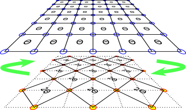
Figure 1: Illustration of chiral gauge transformation. Note the increased unit cell increases flux per plaquette to $2\Theta$. Hamiltonian in Eq. (3) obtained by Fourier Transforming back.

II Rational Transfer Matrix Sequence

Quasi-periodic systems can be readily analyzed with sequences of rational approximates [14]. These are sequences of linear operators whose quasi-periodic parameter, $\alpha\notin\mathbb{Q}$ is replaced by a rational parameter $\frac{p_{n}}{q_{n}}\in\mathbb{Q}$ such that $\lim_{n\rightarrow\infty}\frac{p_{n}}{q_{n}}=\alpha$. The fastest converging sequence is the continued fraction approximation with the n-th approximate defined by

$$\frac{p_{n}}{q_{n}}=a_{0}+\cfrac{1}{a_{1}+\cfrac{1}{\ddots+\cfrac{1}{a_{n}}}}.$$

The golden mean and $\sqrt{2}$ are Diophantine numbers and their continued fraction approximation converges with at worst $|\alpha-\frac{p_{n}}{q_{n}}|<\frac{1}{\sqrt{5}q_{n}^{2}}$ – saturated by the golden mean. By contrast Liouville numbers, are very well approximated by their continued fractions. This means that there exists a $\beta(\alpha)$ such that $|\alpha-\frac{p_{n}}{q_{n}}|<e^{-\beta(\alpha)q_{n}}$. In this work, we focus on the Diophantine case, but these methods can be generalized.

We will take sequences of rational approximate operators by taking the $\Theta=2\pi\alpha$ in Eq. (2) to be its continued fraction approximation $\Theta_{N}=2\pi p_{N}/q_{N}$. For each rational approximate, $H_{N}$, we construct a transfer matrix equation (TME), see [16, 14]. The unit cell for the N-th rational approximate is $q_{N}$ sites long, and a wavefunction on the n-th unit cell is defined by

$$\Psi_{n,N}=\begin{pmatrix}\psi_{n+1}&\ldots&\psi_{n+q_{N}}\end{pmatrix}^{T}.$$ (4)

This translates the eigenvalue equation into a simple form,

$$J_{N}\Psi_{n+1}+M_{N}\Psi_{n}+J_{N}^{\dagger}\Psi_{n-1}=E\Psi_{n}.$$ (5)

Here $J_{N}$ is the hopping matrix connecting the $q_{N}$-th site of $n$-th unit cell to the $1$-st site of the $n+1$-th unit cell, $J_{N}^{\dagger}$ does the opposite, and $M_{N}$ is the intra-unit cell term which acts internally on the $q_{N}$ internal sites of $\Psi_{n}$.

From this we construct a transfer matrix equation (TME),

$$\begin{pmatrix}J_{N}^{-1}(E-M_{N})&-J_{N}^{-1}J_{N}^{\dagger}\\ 1&0\end{pmatrix}\begin{pmatrix}\Psi_{n}\\ \Psi_{n-1}\end{pmatrix}=\begin{pmatrix}\Psi_{n+1}\\ \Psi_{n}\end{pmatrix}.$$ (6)

$J_{N}$ will in general not be invertible, however, we can reduce the transfer matrix in Eq (6), from a $2q_{N}\times 2q_{N}$ matrix to a $2\times 2$ matrix for each rational approximate. The explicit construction of a $2\times 2$ transfer matrix begins with a reduced SVD of the hopping matrix $J_{N}$,

$$J_{N} = V_{N}D_{N}W^{\dagger}_{N}$$ (7)

$$J_{N}^{\dagger} = W_{N}D_{N}^{\dagger}V^{\dagger}_{N}$$ (8)

with $V^{\dagger}V=W^{\dagger}W=\mathbb{1}$ and $W^{\dagger}V=0$, and in the case of $J_{N}$,

$$D_{N}=D_{N}^{\dagger}=\begin{pmatrix}t&0&\ldots&0\\ 0&0&\ldots&0\\ \vdots&\vdots&\ddots&\vdots\\ 0&0&\ldots&0\end{pmatrix},$$ (9)

Since our hopping matrix is rank 1, we truncate $D_{N}=t$ and and correspondingly, the $q_{N}\times 1$ dimensional operators

$$W_{N}^{\dagger}=\begin{pmatrix}0&\ldots&0&(-1)^{q_{N}}\end{pmatrix},V_{N}^{\dagger}=\begin{pmatrix}(-1)^{q_{N}}&0&\ldots&0\end{pmatrix}$$ (10)

Rewriting our intra-unit cell term as a projected Green’s function (pGF)

$$G_{N}(\omega)=(\omega-M_{N})^{-1}$$ (11)

The transfer matrix equation reduces to

$$\Psi_{n} = G_{N}J_{N}\Psi_{n+1}+G_{N}J_{N}^{\dagger}\Psi_{n-1}$$ (12)

$$\Psi_{n} = G_{N}V_{N}D_{N}W^{\dagger}_{N}\Psi_{n+1}+G_{N}W_{N}D_{N}V^{\dagger}_{N}\Psi_{n-1}$$ (13)

Projecting into the $V_{N},W_{N}$ subspaces of $\Psi_{n}$,

$$V^{\dagger}_{N}\Psi_{n} = V^{\dagger}G_{N}V_{N}D_{N}W^{\dagger}_{N}\Psi_{n+1}+V^{\dagger}G_{N}W_{N}D_{N}V^{\dagger}_{N}\Psi_{n-1}$$ (14)

$$W^{\dagger}_{N}\Psi_{n} = W^{\dagger}G_{N}V_{N}D_{N}W^{\dagger}_{N}\Psi_{n+1}+W^{\dagger}G_{N}W_{N}D_{N}V^{\dagger}_{N}\Psi_{n-1}.$$ (15)

This reduces the Transfer matrix equation to [16, 14], setting $t=1$,

$$\begin{pmatrix}(W_{N}^{\dagger}G_{N}V_{N})^{-1}&-(W_{N}^{\dagger}G_{N}V_{N})^{-1}(W_{N}^{\dagger}G_{N}W_{N})\\ (V_{N}^{\dagger}G_{N}V_{N})(W_{N}^{\dagger}G_{N}V_{N})^{-1}&V_{N}^{\dagger}G_{N}W_{N}-V_{N}^{\dagger}G_{N}V_{N}(W_{N}^{\dagger}G_{N}V_{N})^{-1}W_{N}^{\dagger}G_{N}W_{N}\end{pmatrix}\begin{pmatrix}V_{N}^{\dagger}\Psi_{n}\\ W_{N}^{\dagger}\Psi_{n-1}\end{pmatrix}=\begin{pmatrix}V_{N}^{\dagger}\Psi_{n+1}\\ W_{N}^{\dagger}\Psi_{n}\end{pmatrix}$$ (16)

Notice all of the elements in the $2\times 2$ transfer matrix are effectively scalars and thus commute with each other and we can just factor out the common factor $(W_{N}^{\dagger}G_{N}V_{N})^{-1}$,

$$\overbrace{(W_{N}^{\dagger}G_{N}V_{N})^{-1}\begin{pmatrix}1&-(W_{N}^{\dagger}G_{N}W_{N})\\ V_{N}^{\dagger}G_{N}V_{N}&V_{N}^{\dagger}G_{N}W_{N}(W_{N}^{\dagger}G_{N}V_{N})-V_{N}^{\dagger}G_{N}V_{N}W_{N}^{\dagger}G_{N}W_{N}\end{pmatrix}}^{\hat{T}_{q_{N},n}}\begin{pmatrix}V_{N}^{\dagger}\Psi_{n}\\ W_{N}^{\dagger}\Psi_{n-1}\end{pmatrix}=\begin{pmatrix}V_{N}^{\dagger}\Psi_{n+1}\\ W_{N}^{\dagger}\Psi_{n}\end{pmatrix}.$$ (17)

When $W_{N}^{\dagger}G_{N}W_{N}\neq 0$ and $V_{N}^{\dagger}G_{N}V_{N}\neq 0$, $\hat{T}_{q_{N},n}$ is unitary and has reciprocal eigenvalues, $\lambda_{T,1}\lambda_{T,2}=1$. The spectrum, $E\in\Sigma$, is formed by energies for which $\left|\lambda_{T}\right|=1$. By contrast, energies for which $\left|\lambda_{T}\right|\in(0,1)\cup(1,\infty)$ form the spectral gaps, $E\in\mathbb{R}-\Sigma$.

In Eq. 17, zeros of the pGF correspond to $W_{N}^{\dagger}G_{N}W_{N}=0$ (or $V_{N}^{\dagger}G_{N}V_{N}=0$), such that $\hat{T}_{q_{N},n}$ is no longer unitary and $\lambda_{T}=0$ (no normalizeable solutions). The pGF, $G_{N}(\omega)$, thus determines the existence of solutions to the rational approximate TMEs. However, we must check that as $N\rightarrow\infty$, these rational approximates converge to the irrational TME. This reduces to checking that $G_{N}(\omega)\rightarrow(\omega-\hat{H}_{\alpha})^{-1}$ as $N\rightarrow\infty$ [14, 15].

II.1 Projected Green’s Function

In translation-invariant systems, the Brillouin zone allows for flexibility in writing locally computable formulas for topological invariants. In this language, Green’s function zeros are singular and carry topological significance [17, 18, 19, 20, 21, 22, 23, 24, 25]. More recently, it was noticed that bound state formation criteria along an edge are also defined by Green’s function zeros [18, 19, 20, 13, 25, 21], thereby tracking both topological invariants and their corresponding edge modes.

Extending this methodology beyond translation invariant systems consists of two steps. One must show both that Green’s function zeros are still of topological significance and that edge formation criteria are still described by the presence of in-gap zeros. We first show the latter.

The poles of the Green’s function restricted to a particular site in position space correspond to an energy state at that particular site. Here restricted refers to the projection of the system Green’s function, $G$, to a single site,

$$G(\omega,\mathbf{r}_{\perp},\alpha_{\parallel})=\sum_{\alpha}|\mathinner{\langle{\alpha|\mathbf{r}_{\perp}}\rangle}|^{2}G(\omega,\alpha),$$ (18)

where $\alpha$ generically labels the eigenvalues and $\alpha_{\parallel}$ is the remaining index post the contraction with $\mathbf{r}_{\perp}$. Generically, there will be many poles corresponding to the spectrum at $\mathbf{r}_{\perp}$, but they are not universal. By adding on-site impurities and considering $G(\omega,\mathbf{r}_{\perp},\alpha_{\parallel})$ only in the band gap of the bare Green’s function, any poles will be a result of the impurity potential, $\mathcal{V}(r)=\mathcal{V}\delta(r-\mathbf{r}_{\perp})$, binding a state in the gap. We make the impurity bound states into edge modes by tuning the impurity into an edge. This is done by constructing an appropriate impurity geometry and taking $|\mathcal{V}|\rightarrow\infty$. Therefore, the condition for impurity localized states as $|\mathcal{V}|\rightarrow\infty$ is equivalent to the criteria for the formation of edge localized modes.

As $|\mathcal{V}|\rightarrow\infty$, impurity bound states correspond to zeros of the restricted in-gap Green’s function. This is most readily seen by factoring the full Green’s function, $G$ of some system with Hamiltonian $H_{0}$ and an impurity potential $\mathcal{V}$. That is, the full Green’s function $G$ can be written in terms of the Green’s function $G_{0}=(\omega-H_{0})^{\text{-}1}$ of the original system without the impurity,

$$G(\omega,\alpha) = (\omega-(H_{0}+\mathcal{V}))^{\text{-}1}=(1+\mathcal{V}G_{0})^{\text{-}1}G_{0}.$$ (19)

Correspondingly, impurity bound states (poles of $G$) in the gap (not a pole of $G_{0}$) must be a pole of $(1-\mathcal{V}G_{0})^{\text{-}1}$,

$$\det\left[G_{0}(\omega,\alpha)\mathcal{V}-\mathbf{1}\right]=0.$$ (20)

For $|\mathcal{V}|\rightarrow\infty$, solutions require $G_{0}\rightarrow 0$. Hence, the zeros of the restricted in-gap Green’s function, $G(\omega,\mathbf{r}_{\perp},\alpha_{\parallel})$, correspond to edge modes, just as in the translation-invariant case [18].

We show the pGF zeros are still of topological significance in the almost-Mathieu operator by proving the convergence of the rational pGF zeros to the irrational pGF zeros (see below). The rational pGF zeros correspond to deficient points in the transfer matrix equations, thereby defining reducibility classes for the transfer matrix – the deficient point cannot be removed. As such, if the rational pGFs converge to the irrational pGF in an operator norm sense, then the irrational transfer matrix has the same reducibility classes as the limit of the rational sequence generated by the irrational pGF zeros. Proving this convergence for the critical almost-Mathieu operator is non-trivial and requires a special gauge choice (see below).

Thus we define the translation invariant intra-cell projected Green’s function, $G_{N}(\omega)$ in Eq. (17) as

$$\hat{G}_{N}(\omega,\mathbf{k}_{\parallel})=\int d\mathbf{k}_{\perp}G(\omega,\mathbf{k}_{\parallel},\mathbf{k}_{\perp})$$ (21)

where $\mathbf{k}_{\parallel},\mathbf{k}_{\perp}$ represent momenta in parallel and transverse directions to the projection. We then take the limit of $N\rightarrow\infty$, to construct the almost-Mathieu transfer matrix.

II.2 Irrational PGF Zeros and Open Sets

Having constructed irrational pGFs, consider the case where the irrational TME is indeed the convergent limit of the rational TME sequence. In such a case, allowed eigenstates correspond to the limit of rational approximate eigenstates and are effectively invariant under the choice of phase, $\delta$, in Eq. (1) [14, 15].

Lemma 1. If all almost-Mathieu eigenstates are translation invariant, pGF zeros occur if and only if there exists an open complement of the spectrum.

Proof. Consider the pGF for translation invariant eigenstates, and average over all initial sites $x_{0}$ by shifting the phase $\delta$ accordingly

$$G_{\perp,\alpha}(\omega) = \mathinner{\langle{x_{0}}|}\sum_{\xi}G(\omega,\xi)\mathinner{|{\xi}\rangle}\mathinner{\langle{\xi}|}\mathinner{|{x_{0}}\rangle}=\lim_{L\rightarrow\infty}\frac{1}{L}\sum_{x_{0}}\mathinner{\langle{x_{0}}|}\sum_{\xi}G(\omega,\xi)\mathinner{|{\xi}\rangle}\mathinner{\langle{\xi}|}\mathinner{|{x_{0}}\rangle}$$ (22)

$$= \lim_{L\rightarrow\infty}\frac{1}{L}\sum_{\xi}G(\omega,\xi)\mathinner{\langle{\xi}|}(\sum_{x_{0}}\mathinner{|{x_{0}}\rangle}\mathinner{\langle{x_{0}}|})\mathinner{|{\xi}\rangle}=\lim_{L\rightarrow\infty}\frac{1}{L}\sum_{\xi}\frac{1}{\omega-E_{\xi}}$$

Given $\omega$ in a spectral gap between two energies $E_{1}<E_{2}$, $\frac{1}{\omega-E_{1}}>0$ and $\frac{1}{\omega-E_{2}}<0$. Since $\omega$ interopolates between a positive and negative pole, by the Intermediate Value Theorem, it must cross zero. Thus, open sets imply pGF zeros. Note: bulk-boundary correspondence found in [5] follows from this direction.

The reverse direction follows a similar reasoning, assuming the existence of a pGF zero at some $\omega$, this $\omega$ cannot be a pole of $G(\omega,\xi)$, or else we could take an $\omega+i\epsilon$ and then discontinuously remove the zero (see convergence argument below). In the context of the almost-Mathieu operator, this implies that if for some $\omega$, $G_{\perp,\alpha}(\omega)=0$, there must be a ball of radius $\epsilon>0$ for which there are no poles. Otherwise, $\omega$ is the limit point of a sequence of poles and not a pole itself, and the spectrum of $\hat{H}_{\alpha}$ would not contain all of its limit points. However, the almost-Mathieu spectrum is the limit of its rational approximates (see below), and $\omega$ would be the limit of the limit points of a convergent rational sequence. Thus, the almost-Mathieu spectrum must contain its limit points (its spectrum is a Cantor set [13, 7]). This would be a contradiction. Therefore, pGF zeros occur only on open complements of the spectrum. $\hfill\square$

III Almost-Mathieu Convergence

With Lemma 1 in hand, the convergence of the rational pGF sequence to the irrational pGF becomes a connection between the gap topology and open sets in the quasi-periodic spectrum.

Away from the metal-insulator transition, we can choose a magnetic unit cell of the 2D parent Hamiltonian in Eq. (2) such that the rational approximate pGF sequence converges in operator norm to the irrational pGF [14, 15]: for any $\epsilon>0$ there exists an $M\in\mathbb{N}$ such that for $N>M$,

$$||G_{\perp,N}(\omega)-G_{\perp,\alpha}(\omega)||<\epsilon.$$ (23)

However, at criticality, $V=1$ in Eq. (1), the convergence is marginal, [14, 15]. Thus, this parameter regime requires a different gauge choice. To this end, we take advantage of the chiral gauge introduced by Ref. [13] and used by Ref. [2].

III.1 The Chiral Gauge

Defining the operators

$$\hat{V}:\hat{c}^{\dagger}_{x,\delta_{y}}\hat{c}_{x,\delta_{y}}\rightarrow\hat{c}^{\dagger}_{2x,\delta_{y}}\hat{c}_{2x,\delta_{y}}$$ (24)

$$\hat{U}_{a}:\hat{c}^{\dagger}_{x,\delta_{y}}\hat{c}_{x,\delta_{y}}\rightarrow e^{2\pi ixa(\delta_{y}+\Theta/2x)}\hat{c}^{\dagger}_{x,\delta_{y}}\hat{c}_{x,\delta_{y}}$$ (25)

$$\hat{R}:\hat{c}^{\dagger}_{x,\delta_{y}}\hat{c}_{x,\delta_{y}}\rightarrow\sum_{k\in\mathbb{Z}}e^{-2\pi ik(\Theta x+\delta_{y})}\int_{\mathbb{T}}d\beta e^{-2\pi i\beta x}\hat{c}^{\dagger}_{k,\beta}\hat{c}_{k,\beta}$$ (26)

and the composite operator $\hat{Q}=\hat{U}_{1}\hat{R}\hat{U}_{1/2}$, it was shown in [13] that

$$\mathcal{H}_{2D,\Theta}=\hat{Q}\hat{V}^{-1}\mathcal{H}_{ch,\Theta/2}\hat{V}\hat{Q}^{-1}$$ (27)

where $\mathcal{H}_{2D}$ and $\mathcal{H}_{ch}$ are defined in Eq. (2) and Eq. (3) respectively. This highly non-local transformation ($\hat{V}$ maps $x\rightarrow 2x$) is exact and we can construct a rational approximating sequence for $\mathcal{H}_{ch}$,

$$\mathcal{H}_{ch,N}=\sum_{x,\delta_{y}}2\sin{(\pi\frac{p_{N}}{q_{N}}x+\delta_{y})}\hat{c}^{\dagger}_{x+1,\delta_{y}}\hat{c}_{x,\delta_{y}}+2\sin{(\pi\frac{p_{N}}{q_{N}}x+\delta_{y})}\hat{c}_{x+1,\delta_{y}}\hat{c}_{x,\delta_{y}}^{\dagger}$$ (28)

with $\frac{p_{N}}{q_{N}}$ being the $N$-th continued fraction approximation to $\alpha$. This sequence of rational approximate Hamiltonians, $\{\mathcal{H}_{ch,N}\}_{N\in\mathbb{N}}$, generates a sequence of rational approximate pGFs and we can use similar methods as in [14, 15] to prove convergence.

III.1.1 Persistence of pGF Zeros in Chiral Gauge

The chiral gauge choice is arbitrary in 2D, and although it makes the rational approximates appear to be in class AIII, which is general topologically trivial in 2D, the chiral edge modes persist. More precisely, the transformation is only exact for an infinite system, and any rational approximate is translation invariant on the open plane. This translation invariance protects the topological invariant as a stack of chiral 1D models. And, since we are choosing a single $k_{y}$ in our “projection” to the 1D Hamiltonian in Eq. (1), the chiral symmetry actually protects the 1D edge mode even while projecting each of the rational approximates to 1D. Thus, each rational approximate will still have the topologically protected deficient points in its transfer matrix, Eq. 17, for each spectral gap.

III.2 Chiral PGF Convergence

We define the corresponding pGF for each $\mathcal{H}_{ch,N}$,

$$G_{\perp,N}=\int\frac{dk}{2\pi}(\omega-\mathcal{H}_{ch,N})^{-1}.$$ (29)

As done for $\tilde{\mathcal{H}}_{2D}$ in [14, 15], we show $||G_{\perp,N}(\omega)-G_{\perp,\alpha}(\omega)||$ converges for all $\omega$,

$$\left(G_{\perp,N}(\omega)-G_{\perp,\alpha}(\omega)\right) = \int\frac{dk}{2\pi}\left[(\omega-\mathcal{H}_{ch,N})^{-1}-(\omega-\mathcal{H}_{ch,\alpha})^{-1}\right]$$ (30)

$$= \int\frac{dk}{2\pi}\left[\frac{\mathcal{H}_{ch,N}-\mathcal{H}_{ch,\alpha}}{(\omega-\mathcal{H}_{ch,N})^{2}+(\omega-\mathcal{H}_{ch,N})(\mathcal{H}_{ch,N}-\mathcal{H}_{ch,\alpha})}\right].$$

We first bound $\Delta_{N}=||(\mathcal{H}_{ch,N}-\mathcal{H}_{ch,\alpha})||$ by considering

$$|2\sin{(\pi\frac{p_{N}}{q_{N}}x-\delta_{y})}-2\sin{(\pi\alpha x-\delta_{y})}|<2\pi|\frac{p_{N}}{q_{N}}-\alpha|x$$ (31)

At worst for diophantine $\alpha$, $|\frac{p_{N}}{q_{N}}-\alpha|<\frac{1}{\sqrt{5}q_{N}^{2}}$, so

$$|2\sin{(\pi\frac{p_{N}}{q_{N}}x-\delta_{y})}-2\sin{(\pi\alpha x-\delta_{y})}|<\frac{2\pi x}{\sqrt{5}q_{N}^{2}}.$$ (32)

Plugging back into $\Delta_{N}$, we have by Samuelson’s inequality

$$\Delta_{N}<2\sqrt{2\sum_{x=1}^{q_{N}}|2\sin{(\pi\frac{p_{N}}{q_{N}}x-\delta_{y})}-2\sin{(\pi\alpha x-\delta_{y})}|^{2}}<2\sqrt{2\sum_{x=1}^{q_{N}}\left(\frac{\pi x}{\sqrt{5}q_{N}^{2}}\right)^{2}}<2\sqrt{\frac{2\pi^{2}}{30q_{N}}}=2\pi\sqrt{\frac{1}{15q_{N}}}$$ (33)

This bounds the numerator in Eq. (30), but we need to bound the denominator from below as well. This is difficult as the rational spectral gaps become exponentially small in the limit of $N\rightarrow\infty$ [26, 13]. We avoid this problem by considering a small deviation into the complex plane to bound $(\omega\pm i\epsilon-\mathcal{H}_{ch,N})^{-1}<|\epsilon|$, by the Hermiticity of $\mathcal{H}_{ch,N}$.

III.2.1 Complex pGF Convergence

We consider $\omega\rightarrow\omega\pm i\epsilon$ and prove that for any $\epsilon>0$, we can take $q_{N}$ sufficiently large such that for any $\delta>0$

$$||\mathrm{Re}\,(G_{\perp,\alpha}(\omega\pm i\epsilon)-G_{\perp,N}(\omega\pm i\epsilon))|| < \delta,\quad||\mathrm{Im}\,(G_{\perp,\alpha}(\omega\pm i\epsilon)-G_{\perp,N}(\omega\pm i\epsilon))||<\delta.$$ (34)

Or,

$$\lim_{\epsilon\rightarrow 0}\lim_{q_{N}\rightarrow\infty}||G_{\perp,\alpha}(\omega\pm i\epsilon)-G_{\perp,N}(\omega\pm i\epsilon)||=0.$$ (35)

As the Green’s function is continuous on the upper and lower half of the complex plane, with the same limit,

$$\lim_{q_{N}\rightarrow\infty}||G_{\perp,\alpha}(\omega)-G_{\perp,N}(\omega)||=0.$$ (36)

We need the real and imaginary parts to converge separately,

$$\mathrm{Re}\,{(G_{\perp,\alpha}(\omega\pm i\epsilon)-G_{\perp,N}(\omega\pm i\epsilon))}=-\int\frac{dk}{2\pi}\frac{\left[(\omega-\tilde{H}_{ch,N})^{2}+(\omega-\tilde{H}_{ch,N})(\tilde{H}_{ch,N}-\tilde{H}_{ch,\alpha})-\epsilon^{2}\right](\tilde{H}_{ch,\alpha}-\tilde{H}_{ch,N})}{((\omega-\tilde{H}_{ch,N})^{2}+\epsilon^{2})^{2}\left(\mathbb{1}+\frac{2\omega(H_{ch,N}-H_{\alpha})+\tilde{H}_{ch,N}^{2}-\tilde{H}_{ch,\alpha}^{2}}{((\omega-\tilde{H}_{ch,N})^{2}+\epsilon^{2})}\right)}$$ (37)

$$\mathrm{Re}\,{(G_{\perp,\alpha}(\omega\pm i\epsilon)-G_{\perp,N}(\omega\pm i\epsilon))}=-\int\frac{dk}{2\pi}\frac{(\tilde{H}_{ch,\alpha}-\tilde{H}_{ch,N})}{((\omega-\tilde{H}_{ch,N})^{2}+\epsilon^{2})\left(\mathbb{1}+\frac{2\omega(H_{ch,N}-H_{\alpha})+\tilde{H}_{ch,N}^{2}-\tilde{H}_{ch,\alpha}^{2}}{((\omega-\tilde{H}_{ch,N})^{2}+\epsilon^{2})}\right)}$$

$$-\int\frac{dk}{2\pi}\frac{\left[(\omega-\tilde{H}_{ch,N})(\tilde{H}_{ch,N}-\tilde{H}_{ch,\alpha})-2\epsilon^{2}\right](\tilde{H}_{ch,\alpha}-\tilde{H}_{ch,N})}{((\omega-\tilde{H}_{ch,N})^{2}+\epsilon^{2})^{2}\left(\mathbb{1}+\frac{2\omega(H_{ch,N}-H_{\alpha})+\tilde{H}_{ch,N}^{2}-\tilde{H}_{ch,\alpha}^{2}}{((\omega-\tilde{H}_{ch,N})^{2}+\epsilon^{2})}\right)}$$ (38)

$$\mathrm{Im}\,{(G_{\perp,\alpha}(\omega\pm i\epsilon)-G_{\perp,N}(\omega\pm i\epsilon))}=\int\frac{dk}{2\pi}\frac{\left[\pm 2i\epsilon(\omega-\tilde{H}_{ch,N})+i\epsilon(H_{ch,N}-\tilde{H}_{ch,\alpha})\right](\tilde{H}_{ch,\alpha}-\tilde{H}_{ch,N})}{((\omega-\tilde{H}_{ch,N})^{2}+\epsilon^{2})^{2}\left(\mathbb{1}+\frac{2\omega(H_{ch,N}-H_{\alpha})+\tilde{H}_{ch,N}^{2}-\tilde{H}_{ch,\alpha}^{2}}{((\omega-\tilde{H}_{ch,N})^{2}+\epsilon^{2})}\right)}$$

$$\mathrm{Im}\,{(G_{\perp,\alpha}(\omega\pm i\epsilon)-G_{\perp,N}(\omega\pm i\epsilon))}=\int\frac{dk}{2\pi}\frac{2i\epsilon(\tilde{H}_{ch,\alpha}-\tilde{H}_{ch,N})}{((\omega-\tilde{H}_{ch,N})^{2}+\epsilon^{2})((\omega-\tilde{H}_{ch,N})\pm i\epsilon)\left(\mathbb{1}+\frac{2\omega(H_{ch,N}-H_{\alpha})+\tilde{H}_{ch,N}^{2}-\tilde{H}_{ch,\alpha}^{2}}{((\omega-\tilde{H}_{ch,N})^{2}+\epsilon^{2})}\right)}$$

$$+\int\frac{dk}{2\pi}\frac{\left[2\epsilon^{2}+i\epsilon(H_{ch,N}-\tilde{H}_{ch,\alpha})\right](\tilde{H}_{ch,\alpha}-\tilde{H}_{ch,N})}{((\omega-\tilde{H}_{ch,N})^{2}+\epsilon^{2})^{2}\left(\mathbb{1}+\frac{2\omega(H_{ch,N}-H_{\alpha})+\tilde{H}_{ch,N}^{2}-\tilde{H}_{ch,\alpha}^{2}}{((\omega-\tilde{H}_{ch,N})^{2}+\epsilon^{2})}\right)}.$$ (39)

Now we use that $||(\omega-\tilde{H}_{ch,N})^{2}+\epsilon^{2}||>\epsilon^{2}$, to cancel the bottom factors $\sim\frac{1}{\epsilon^{2}}$. And, we can use the bound from above, $||\tilde{H}_{ch,N}-\tilde{H}_{ch,\alpha}||<2\pi\sqrt{\frac{1}{15q_{N}}}$ to get

$$||\mathrm{Re}\,{(G_{\perp,\alpha}(\omega\pm i\epsilon)-G_{\perp,N}(\omega\pm i\epsilon))}||<\int\frac{dk}{2\pi}||\epsilon^{-4}\left[-\epsilon^{2}2\pi\sqrt{\frac{1}{15q_{N}}}+(\omega-\tilde{H}_{ch,N})\left(2\pi\sqrt{\frac{1}{15q_{N}}}\right)^{2}\right]||$$ (40)

$$||\mathrm{Im}\,{(G_{\perp,\alpha}(\omega\pm i\epsilon)-G_{\perp,N}(\omega\pm i\epsilon))}||<\int\frac{dk}{2\pi}\epsilon^{-3}\left[\epsilon 8\pi\sqrt{\frac{1}{15q_{N}}}+\left(2\pi\sqrt{\frac{1}{15q_{N}}}\right)^{2}\right].$$ (41)

Clearly the imaginary part will converge to zero for large $q_{N}$. We bound the real part by showing

$$||(\omega-\tilde{H}_{ch,N})||<C\sqrt{q_{N}},$$ (42)

so that we can always take $q_{N}$ big enough to make $\left(2\pi\sqrt{\frac{1}{15q_{N}}}\right)^{2}C\sqrt{q_{N}}<\epsilon^{4}$ for any $\epsilon>0$ to get the uniform convergence above, for all Diophantine $\alpha$.

Thus, the inequalities in Eq. (34) reduce to bounding $||(\omega-H_{ch,N})||$, and the operator norm obeys the triangle inequality. So,

$$||(\omega-\tilde{H}_{ch,N})||\leq|\omega|+||\tilde{H}_{ch,N}||$$ (43)

We the use Samuelson’s inequality to bound the chiral gauge eigenvalues. Notice that the characteristic polynomial of $\tilde{H}_{ch,N}$ has the coefficients

$$P_{N}(\lambda)=\lambda^{q_{N}}+0\lambda^{q_{N}-1}-\sum_{i=1}^{q_{N}}4\sin^{2}{(\pi\frac{p_{N}}{q_{N}}i-\delta_{y})}\lambda^{q_{N}-2}+\ldots+\det{\tilde{H}_{ch,N}}\lambda^{0}$$ (44)

Therefore, by Samuelson’s inequality, the largest eigenvalue and consequentially the operator norm is at most,

$$||\tilde{H}_{ch,N}||<2\sqrt{2\sum_{i=1}^{q_{N}}\sin^{2}{(\pi\frac{p_{N}}{q_{N}}i-\delta_{y})}}=2\sqrt{q_{N}}$$ (45)

and thus

$$||\mathrm{Re}\,{(G_{\perp,\alpha}(\omega\pm i\epsilon)-G_{\perp,N}(\omega\pm i\epsilon))}||<\left[\epsilon^{-2}2\pi\sqrt{\frac{1}{15q_{N}}}+\epsilon^{-4}(|\omega|+2\sqrt{q_{N}})\left(2\pi\sqrt{\frac{1}{15q_{N}}}\right)^{2}\right].$$ (46)

Then, choosing $q_{N}>\epsilon^{-4}\delta^{-2}$,

$$||\mathrm{Re}\,{(G_{\perp,\alpha}(\omega\pm i\epsilon)-G_{\perp,N}(\omega\pm i\epsilon))}||<\delta,\quad||\mathrm{Im}\,{(G_{\perp,\alpha}(\omega\pm i\epsilon)-G_{\perp,N}(\omega\pm i\epsilon))}||<\delta,$$ (47)

as desired. $\hfill\square$

III.3 Effective Translation Invariance

The pGF convergence proven in Section III.2 directly implies the rational transfer matrix equation converges to the irrational transfer matrix equation (TME). Thus, if they exist, the eigenfunctions for the critical almost-Mathieu operator, defined as the limit points of the rational sequence, are in fact the irrational limit of the rational approximate eigenfunctions.

The initial choice of phase $\delta$ in Eq. 1 can be absorbed by choosing a different starting point from which to approximate the irrational TME, i.e. $\cos{[\Theta x+\delta]}=\cos{[\Theta(x-1)+\delta+\theta]}$. Since the the irrational TME is the limit of the rational TME, these phase shifts are absorbed by the rational sequence. The rational eigenfunctions are thus effectively invariant under these phase shifts, and consequentially, their limit is invariant as well. However, in 1D these phase shifts amount to translations of the lattice. Therefore, the critical almost-Mathieu operator has translation invariant eigenfunctions and Lemma 1 applies.

IV Dry Ten Martini Problem

We restate the problem statement for convenience:

Dry Ten Martini Problem. Consider an energy in the spectrum of the critical almost-Mathieu operator $E\in\Sigma$, satisfying $\hat{H}\mathinner{|{\psi}\rangle}=E\mathinner{|{\psi}\rangle}$ with $\hat{H}$ as in Eq. (1) and $V=1$. If $N(E)=m\alpha+n$ with $m,n\in\mathbb{Z}$ and $\Theta=2\pi\alpha\in$, then E belongs to the boundary of a component of $\mathbb{R}-\Sigma$.

Proof. As discussed in Section III.3, the convergence of the rational transfer matrix sequence to the irrational transfer matrix, implies the almost-Mathieu eigenfunctions are invariant under phase shifts $\delta\rightarrow\delta+\Theta$ and Lemma 1 holds. So, we combine Lemma 1 with the transfer matrix results above.

First, by the convergence proof above, all eigenvalues of the irrational pGF are generated by the limit of rational 2D approximates, including zeros. Thus all irrational pGF zeros are generated by zeros occurring in spectral gaps of rational approximates. Then, by Lemma 1, the sequence of rational pGF zeros form open sets in the compliment of the almost-Mathieu operator spectrum $\mathbb{R}-\Sigma$.

Second, for any rational approximate, each gap has a non-trivial Chern number thanks to the magnetic flux per plaquette, even in the chiral gauge, Section III.1.1. By the results in [5, 27, 9], these Chern numbers (slopes) form the irrational gap-labels in the continued fraction limit. Bulk-boundary correspondence [28, 29, 5] implies the existence of edge modes (pGF zeros) corresponding to the non-trivial Chern numbers in each gap. So, for any gap labeled by the gap-labeling theorem, we can take a large enough rational approximate, $q_{N}$, such that for all future approximates the rational band gap with the same label has a pGF zero. Thus, for large enough $q_{N}$, and any gaps labeled by the gap-labeling theorem, there exists an $\omega_{g}$ in the gap, such that $G_{\perp,\alpha}(\omega_{g})=0$.

Together, these statements imply that every gap-labeling theorem labeled ”gap” will form an open set in the compliment of the almost-Mathieu spectrum, $\mathbb{R}-\Sigma$. Or, as phrased above, if the density of states $N(E)=m\Theta+n$, then $E$ must form the boundary of an open set. $\hfill\square$

V Conclusion

In summary, the central idea in this work was the construction of the almost-Mathieu transfer matrix from a sequence of rational approximate transfer matrices using the reduced SVD approach in [16, 14, 15]. The projected Green’s functions appear as a consequence of the reduced SVD method and allow us to import powerful ideas from band topology to show the spectral gaps form open sets. A clear benefit of this approach is the geometric intuition provided by the rational approximates, which can be readily extended to other quasi-periodic patterns, see [14].

While only a single point in parameter space, the critical almost-Mathieu operator is precisely the isotropic Hofstadter Hamiltonian. And, since there is an irrational flux arbitrarily close to any rational flux (irrationals are dense in the reals), the dry ten martini problem asks whether or not topological invariants are stable for IQHE on a lattice. We push the answer to the affirmative.

References

• Aubry and André [1980] S. Aubry and G. André, Soc. 3, 133 (1980).
• Jitomirskaya [2021] S. Jitomirskaya, Advances in Mathematics 392, 107997 (2021).
• Jitomirskaya and Last [1998] S. Y. Jitomirskaya and Y. Last, Communications in mathematical physics 195, 1 (1998).
• Bellissard et al. [1982] J. Bellissard, A. Formoso, R. Lima, and D. Testard, Physical Review B 26, 3024 (1982).
• Prodan [2015] E. Prodan, Phys. Rev. B 91, 245104 (2015).
• Kraus et al. [2012] Y. E. Kraus, Y. Lahini, Z. Ringel, M. Verbin, and O. Zilberberg, Physical review letters 109, 106402 (2012).
• Avila and Jitomirskaya [2009] A. Avila and S. Jitomirskaya, Annals of mathematics , 303 (2009).
• Avila and Krikorian [2006] A. Avila and R. Krikorian, Annals of Mathematics , 911 (2006).
• BELLISSARD [1986] J. BELLISSARD, Lecture Notes in Physics 257, 99 (1986).
• Han [2018] R. Han, Transactions of the American Mathematical Society 370, 197 (2018).
• Avila and Jitomirskaya [2011] A. Avila and S. Jitomirskaya, Communications in mathematical physics 301, 563 (2011).
• Jitomirskaya and Marx [2012] S. Jitomirskaya and C. Marx, Geometric and Functional Analysis 22, 1407 (2012).
• Jitomirskaya and Krasovsky [2019] S. Jitomirskaya and I. Krasovsky, Critical almost mathieu operator: hidden singularity, gap continuity, and the hausdorff dimension of the spectrum (2019), arXiv:1909.04429 [math.SP] .
• Borgnia et al. [2021] D. S. Borgnia, A. Vishwanath, and R.-J. Slager, arXiv preprint arXiv:2109.13933  (2021).
• Borgnia and Slager [2021] D. S. Borgnia and R.-J. Slager, arXiv preprint arXiv:2111.02789  (2021).
• Dwivedi and Chua [2016] V. Dwivedi and V. Chua, Physical Review B 93, 134304 (2016).
• Bernevig and Hughes [2013] B. A. Bernevig and T. L. Hughes, Topological insulators and topological superconductors (Princeton university press, 2013).
• Slager et al. [2015] R.-J. Slager, L. Rademaker, J. Zaanen, and L. Balents, Physical Review B 92, 085126 (2015).
• Rhim et al. [2018] J.-W. Rhim, J. H. Bardarson, and R.-J. Slager, Phys. Rev. B 97, 115143 (2018).
• Borgnia et al. [2020] D. S. Borgnia, A. J. Kruchkov, and R.-J. Slager, Phys. Rev. Lett. 124, 056802 (2020).
• Volovik [2003] G. E. Volovik, The universe in a helium droplet, Vol. 117 (Oxford University Press on Demand, 2003).
• Bouhon et al. [2019] A. Bouhon, A. M. Black-Schaffer, and R.-J. Slager, Phys. Rev. B 100, 195135 (2019).
• Slager [2019] R.-J. Slager, Journal of Physics and Chemistry of Solids 128, 24 (2019).
• Gurarie [2011] V. Gurarie, Phys. Rev. B 83, 085426 (2011).
• Mong and Shivamoggi [2011] R. S. Mong and V. Shivamoggi, Physical Review B 83, 125109 (2011).
• Jitomirskaya et al. [2020] S. Jitomirskaya, L. Konstantinov, and I. Krasovsky, arXiv preprint arXiv:2007.01005  (2020).
• Bourne and Prodan [2018] C. Bourne and E. Prodan, Journal of Physics A: Mathematical and Theoretical 51, 235202 (2018).
• Halperin [1982] B. I. Halperin, Physical Review B 25, 2185 (1982).
• Bellissard [1986] J. Bellissard, in Statistical mechanics and field theory: mathematical aspects (Springer, 1986) pp. 99–156.