The whole and the parts: the MDL principle and the a-contrario framework

Abstract

This work explores the connections between the Minimum Description Length (MDL) principle as developed by Rissanen, and the a-contrario framework for structure detection proposed by Desolneux, Moisan and Morel. The MDL principle focuses on the best interpretation for the whole data while the a-contrario approach concentrates on detecting parts of the data with anomalous statistics. Although framed in different theoretical formalisms, we show that both methodologies share many common concepts and tools in their machinery and yield very similar formulations in a number of interesting scenarios ranging from simple toy examples to practical applications such as polygonal approximation of curves and line segment detection in images. We also formulate the conditions under which both approaches are formally equivalent.

62H35, 94A13

1 Introduction

The Minimum Description Length principle (MDL), introduced by Rissanen in 1978 [26] and further developed in [2, 18, 27, 28, 29], is an information-theoretic approach to the statistical problem of Model Selection. The MDL principle was developed as a practical, computable approach to the Algorithmic Information Theory developed by Solomonoff [30, 31], Kolmogorov [22] and Chaitin [3, 4]. It was later significantly improved by the development of Universal Coding Theory [6], a powerful generalization of the optimal coding methods developed by Shannon, Fano, Elias and Huffmann.

The a-contrario detection theory was developed by Desolneux, Moisan and Morel [10, 11] and is based on a statistical formulation of the non-accidentalness principle [1, 33]. Its aim is to control the expected number of false detections under random conditions. Its rationale is that events likely to arise by accident should not be considered meaningful detections and must be rejected. In other words, only significant deviations from randomness are meaningful.

The theoretical and philosophical foundations of both approaches are very different. As the name suggest, the Minimum Description Length principle follows the same basic idea of Algorithmic Complexity, preferring the model that leads to the shortest description of the whole data. The non-accidentalness principle, on the other hand, suggests rejecting events that are expected to be observed in random data. The former considers a global description whereas the latter concentrates on the detection of anomalous structures present in the data.

Despite their different formulations, both methods find common ground in one important case: uniformly distributed random data (without loss of generality, over a finite alphabet). According to Kolmogorov’s definition, the shortest description of such data will be as long as the data itself with overwhelming probability. In other words, when the data is random, no clever model can be devised which allows for a more compact description than spelling out the data itself. In MDL, such data is non-compressible and thus the best model is the uniform distribution. In the context of a detection problem this constitutes a non-detection. As for a-contrario, the non-accidentalness principle also guarantees that no detection will occur in this scenario.

This work seeks to show that similarities between both approaches exist beyond the aforementioned case. We demonstrate this in various examples, ranging from simple problems, where we can perform an in-depth analysis of the expressions involved, to more complex real applications where we show, by experimentation, that both methodologies indeed produce very similar results. In particular, we develop and evaluate automatic methods to choose the “best” polygonal approximation of a given object, and for detecting line segments, using both criteria. Finally, we establish certain conditions under which both approaches are equivalent.

The MDL principle is mainly a model selection tool, but can also be used as a detection criterion. On the other hand, the a-contrario framework was mainly proposed as a detection criterion, but can also be used for model selection. Thus, both methodologies can be applied to a large range of similar applications, facilitating the comparison. Also, both methodologies require a modeling step. In all cases, from toy examples to real applications, our results show that both a-contrario and MDL give very similar results whenever similar modeling criteria are used.

The rest of this document is organized as follows. The basic common notation and concepts are introduced in Section 2. Then, Section 3 provides a self-contained, concise introduction to the MDL principle, starting with its Algorithmic Information Theory foundations, and the key tools in Universal Coding Theory which enable its application in practice. Section 4 does the same with the a-contrario theory. Section 5 compares both approaches in a first toy setting: detecting an individual square on a noisy image. Section 6 moves to the more interesting case of detecting many squares. Next, two more complex problems are addressed. Section 7, deals with the selection of the best polynomial approximation to a curve; this is a typical model selection problem for which MDL was specifically developed. Section 8, deals with detection of line segments in images; this, in turn, is a typical computer vision application of the a-contrario approach. Then, Section 9 establishes the theoretical conditions under which both approaches are equivalent. Final comments and perspectives are given in Section 10 and Section 11.

2 Notation, conventions and common concepts

In this brief preamble we summarize the meaning of common terms and symbols used throughout the document. The object of our study will be a data vector $\mathbf{x}=(x_{1},x_{2},\ldots,x_{n})$ of length $n$ where each $x_{i}$ takes values in a finite alphabet $\mathcal{X}$ of size $|\mathcal{X}|$; here $|\cdot|$ denotes the cardinality operator. Images will be treated in the same way by concatenating their rows into a single vector. Without loss of generality, we will assume that all images are of size $\sqrt{n}\times\sqrt{n}$.

When the nature of $\mathbf{x}$ is assumed stochastic, $\mathbf{X}$ denotes the random vector associated to it, and $X_{i}$ represents the random variable corresponding to the i-th sample of $\mathbf{x}$, $x_{i}$.

All the examples of this work involve analyzing parts of the (whole) data vector $\mathbf{x}$. We define a part $\mathbf{x}_{i}$ of $\mathbf{x}$ to be an arbitrary non-empty subset of elements of $\mathbf{x}$: $\mathbf{x}_{i}=\{x_{j_{1}},\ldots,x_{j_{n_{i}}}\}$ where $j_{k}$ are the indexes of the elements and $n_{i}$ is the size of the part. In general, we may analyze several different parts of the data simultaneously. Let $\{\mathbf{x}_{1},\ldots,\mathbf{x}_{N}\}$ be a set of $N$ parts of $\mathbf{x}$ in which we are interested. This set of parts is not necessarily a partition: it does not need to cover the whole $\mathbf{x}$, and different parts may overlap. For example, if $\mathbf{x}$ is an image, the parts $\{\mathbf{x}_{i}:i=1.\ldots,N\}$ may correspond to a group of selected (possibly overlapping) patches. For a particular part, the value of $\mathbf{x}_{i}$ will vary for different realizations of $\mathbf{x}$. We say that a configuration is a particular realization of a given part. If $\mathbf{x}$ is stochastic, $\mathbf{X}_{i}$ represents the random vector associated to part $\mathbf{x}_{i}$.

Parts are the subject of the tests conducted in this work. When dealing with detection problems, our goal will be to determine whether a part stands out from the background or not. In that case, we declare a detection. Otherwise, no detection is declared. In such scenarios, a “background” model is assumed. This can be, for example, a distribution on $\mathbf{x}$, such as the uniform distribution over $\mathcal{X}^{n}$. In general, we associate a model to an hypothesis. In the case of detections, the background model is associated to the null hypothesis $H_{0}$ (i.e., the part is part of the background), and the non-null hypothesis $H_{1}$ corresponds to a detection.

In model selection problems, many different models (hypotheses) are proposed for a given part; the background model (null hypothesis) is always included among these. Note that, as formulated, the detection problem is a special case of a model selection problem where only one non-null hypothesis is formulated.

In any case, the decision on a part is made by computing a score for each model and selecting the one with the best score. A score is a function of the model, the part, and its configuration. However, how exactly this score function is constructed depends on many factors. Most of the technical work in this paper is devoted to constructing this function.

3 The Minimum Description Length principle

The Model Selection problem can be stated as follows: which is the best model to describe a given data? This is a fundamental problem in Statistics and Science as a whole. In its most general formulation (any possible model), this problem is unsolvable [22, 24]. Therefore, the effort has been focused on selecting the best model from sets of structured candidates.

The Minimum Description Length [18] has its philosophical roots in the famous “Occam’s Razor” principle, whose modern interpretation can be summarized by saying that, being equally precise, simpler explanations should be preferred over complex ones. To weight different explanations, MDL draws from the theory of Algorithmic Complexity (also known as Kolmogorov complexity) [24]. This theory, developed independently by Solomonoff [30, 31], Kolmogorov [22] and Chaitin [3, 4], states that the complexity of a data object is given by the shortest program that can describe it using a Universal Turing Machine.

In accordance with the unsolvability of the general Model Selection problem, it has long been shown that finding the shorter program to describe a given data is a non-computable problem [34]. In view of this difficulty, the MDL principle reduces its search to a set of candidate descriptions that are easy to evaluate: this is usually a family $\mathcal{M}$ of parametric probability models and a method for compressing data using these models. In short, given some data, MDL will choose the model $M\in\mathcal{M}$ which, when fed to the compression algorithm, yields the shortest description for that data. The choice of the family of models $\mathcal{M}$ for a particular problem is the modeling step.

Given $\mathcal{M}$, the problem of designing an algorithm which will produce the shortest possible description of any given data using the available models in $\mathcal{M}$ is non-trivial. This is the subject of Universal Coding Theory (UC) [6]; much of the literature on MDL deals with the design and implementation of such algorithms. Whereas the traditional (pre-Universal) Coding Theory deals with developing compression algorithms for sources with fully known probability distributions, UC deals with the problem of encoding data whose distribution is assumed known only in its general form (e.g., “a polynomial plus Gaussian noise” or a “Markov Process of arbitrary order”).

More Formally, let $\mathcal{M}=\{M_{\theta}:\theta\in\Theta\}$ be a family of probability models defined over $\mathbf{x}$ indexed by a parameter $\theta$. We denote by $L_{\mathcal{M}}(\mathbf{x}|M_{\theta})$ the code-length assigned by model $M_{\theta}$ to $\mathbf{x}$. To produce a complete description of $\mathbf{x}$, $M_{\theta}$ needs to be encoded as well; we denote the joint encoding of $\mathbf{x}$ and $M_{\theta}$ given the family as $L_{\mathcal{M}}(\mathbf{x},M_{\theta})$ (the family $\mathcal{M}$ is unique and known both to the encoder and the decoder, so there is no need to describe it when transmitting $\mathbf{x}$):

(1) $$L_{\mathcal{M}}(\mathbf{x},M_{\theta})=L_{\mathcal{M}}(\mathbf{x}|M_{\theta})+L_{\mathcal{M}}(M_{\theta}).$$

The two terms in (1) play the role of a fitting term and a penalty term, respectively, in traditional regularization methods. It is not necessary to actually encode the data in a binary stream; only code-lengths matter. However, the code-length assignments need to be valid. A central theorem in Information Theory (see [6]) establishes that any valid code-length assignment needs to satisfy the Kraft inequality [8]:

$$\sum_{\mathbf{x}\in\mathcal{X}^{n}}2^{-L_{\mathcal{M}}(\mathbf{x},M_{\theta})}\leq 1.$$

The main problem with the original (called “two-parts”) formulation of MDL [26] is the arbitrariness in separating $L_{\mathcal{M}}(\mathbf{x},M_{\theta})$ into $L_{\mathcal{M}}(\mathbf{x}|M_{\theta})$ and $L_{\mathcal{M}}(M_{\theta})$; as soon as one wants to describe the model parameter $\theta$, one faces the problem of choosing a model for $\theta$ itself.

A fundamental development in MDL was the incorporation of tools from the Universal Coding, which allow for a provably optimal, one-part encoding of $\mathbf{x}$ directly in terms of the whole family $\mathcal{M}$: $L_{\mathcal{M}}(\mathbf{x})$. In these schemes, the parameter $\theta$ is “marginalized-out”. A fundamental result [27] states that $L_{\mathcal{M}}(\mathbf{x})$ can still be decomposed into two terms (not to be confused with the two-parts coding mentioned earlier):

$$L_{\mathcal{M}}(\mathbf{x})=L(\mathbf{x}|\mathcal{M})+L(\mathcal{M}).$$

The term $L(\mathcal{M})$ is called Model Complexity and depends solely on the size and richness of the model itself: larger model families are inherently more complex and thus result in a larger, unavoidable overhead, no matter the encoding in use. The term $L(\mathbf{x}|\mathcal{M})$, called Stochastic Complexity, depends on the particularities of the data $\mathbf{x}$ to be encoded. Again, these two terms play the roles of regularization and fitting terms, even though the division is not explicit.

The proper application of modern MDL requires one to develop an optimal one-part coding scheme. In many cases, however, such schemes are impractical to implement, and one must settle for an imperfect two-parts coding approach. In such cases (besides complying with the Kraft inequality), the only sanity check is that the actual code-lengths produced are better than those obtained by a trivial, raw encoding for the data that one is working with (e.g., if one wants to encode digital images of $n$ pixels with $8$ bits per pixel, a useful code should produce code-lengths well below $8n$ bits for most images).

4 The a-contrario framework

The a-contrario framework was introduced by Desolneux, Moisan and Morel [10, 11] as a general way of selecting detection thresholds while controlling the number of false detections under a background or null hypothesis $H_{0}$. It can be seen as a formalization of the non-accidentalness principle [1, 33] which states that an observed structure is meaningful only when the relationship between its elements is too regular to be the result of an accidental arrangement of independent elements. The idea is illustrated informally in the following passage:

For so many people connected with the Armstrong case to be travelling by the same train through coincidence was not only unlikely: it was impossible. It must be not chance, but design.
Agatha Christie, “Murder on the Orient Express”

or even in the more concise words of Ian Fleming in “Goldfinger”: Once is happenstance. Twice is coincidence. The third time it’s enemy action. Both quotes suggest the idea that a large number of coincidences implies a common cause. D. Lowe expressed the same idea more formally in the context of pattern detection in digital images:

we need to determine the probability that each relation in the image could have arisen by accident, $P(a)$. Naturally, the smaller that this value is, the more likely the relation is to have a causal interpretation.
David Lowe [25, p. 39]

The same idea is the basis of hypothesis testing in statistics.

The a-contrario approach aims at detecting parts of the data with anomalous statistics. The a-contrario formulation requires: (a) a family of events or parts to be analysed; (b) a function $\xi(\mathbf{x}_{i})$ providing the degree of anomalousness of a data part $\mathbf{x}_{i}$; (c) a stochastic model $H_{0}$ for random data. The latter determines the distribution of random data, which in turn allows to evaluate whether a given event is common or rare.

The function $\xi$ acts on parts $\mathbf{x}_{i}$ and produces a real number $y_{i}=\xi(\mathbf{x}_{i})$. This function introduces an order among all possible configurations of $\mathbf{x}_{i}$, determining the sense in which a vector will be considered anomalous. A vector with a large enough $y_{i}$ value will be considered anomalous. To give an example, in an image, patches with large average pixel values may be considered anomalous. Finally, a stochastic model $H_{0}$ is required for background data; a piece of data $\mathbf{x}_{i}$ will be considered anomalous when observing the value $y_{i}=\xi(\mathbf{x}_{i})$ or a larger one is a rare event under $H_{0}$. In some settings, there is a natural stochastic model $H_{0}$ for unstructured data; we will see some examples later. In the absence of particular reasons to specify a model $H_{0}$, we can follow Laplace’s principle of indifference and assume that all possible realizations of the data vector are equally probable under $H_{0}$. Correspondingly, let $\mathbf{X}_{i}$ denote the random vector associated with a part $\mathbf{x}_{i}$ and $Y_{i}=\xi(\mathbf{X}_{i})$.

We are now ready to introduce the main ideas of the a-contrario approach. The formalism is based on a multiple test procedure as used in statistics [20] and is very similar to the procedure in [13]. We want a criterion $F$ such that detections are declared when $F(i,y_{i})\leq\varepsilon$ for a fixed value $\varepsilon$. The main idea of the a-contrario approach is to design $F$ to control the expected number of detections under $H_{0}$; i.e., when $F$ is applied to random variables $Y_{i}$. In such conditions, any detection would be a false detection. Here, we will follow the formulation introduced in [17].

Definition 4.1 (Grosjean-Moisan [17]).

Let $\{Y_{1},\ldots,Y_{N}\}$ be a set of $N$ random variables. A function $F(i,y)$ is a NFA (Number of False Alarms) for the random variables $\{Y_{i}\}$ if

(2) $$\forall\varepsilon>0,\quad\mathbb{E}\left[\sum_{i=1}^{N}\mathbb{1}_{F(i,Y_{i})\leq\varepsilon}\right]\leq\varepsilon.$$

In words, the condition in Equation 2 implies that the expected number of random variables satisfying $F(i,Y_{i})\leq\varepsilon$ is bounded by $\varepsilon$; this condition is equivalent to

(3) $$\sum_{i=1}^{N}\mathbb{P}\big{(}F(i,Y_{i})\leq\varepsilon\big{)}\leq\varepsilon.$$

A function $F$ satisfying  Definition 4.1 ensures that the average number of false detections under $H_{0}$ is less than $\varepsilon$. Thus, a NFA allows controlling the global number of false detections by making detections only when $F(i,y)\leq\varepsilon$ for the observed value $y$.

Proposition 4.2 (Grosjean-Moisan [17]).

Let $\{Y_{1},\ldots,Y_{N}\}$ be a set of $N$ random variables and $\{\eta_{1},\ldots,\eta_{N}\}$ a set of positive real numbers such that

(4) $$\sum_{i=1}^{N}\frac{1}{\eta_{i}}\leq 1.$$

Then, the function

(5) $$F(i,y)=\eta_{i}\cdot\mathbb{P}[Y_{i}\geq y]$$

is an NFA.

The condition $\sum_{i=1}^{N}\frac{1}{\eta_{i}}\leq 1$ allows to apply a different confidence level $\varepsilon/\eta_{i}$ to each test while still controlling the average number of false detections by $\varepsilon$. In short, a detection will be declared in part $\mathbf{x}_{i}$ if

(6) $$\mathrm{NFA}_{i}=\eta_{i}\cdot\mathbb{P}\big{[}\xi(\mathbf{X}_{i})\geq\xi(\mathbf{x}_{i})\big{]}\leq\varepsilon,$$

where $\varepsilon$ is a fixed value indicating the average number of false detections one is ready to accept when $\mathbf{x}$ is a realization of $\mathbf{X}\sim H_{0}$. In particular, setting $\eta_{i}=N$ for all $i$ (which corresponds to the Bonferroni correction in multiple test settings), assigns the same risk $\varepsilon/N$ to each test, while keeping the average number of false detections below $\varepsilon$. In many practical applications the value $\varepsilon=1$ is adopted. Indeed, it allows for less than one false detection per data (for example an image), which is usually quite tolerable.

A few comments are now in place. First, we are following the setting of Section 2, so the elements of $\mathbf{x}$ take values in a finite alphabet $\mathcal{X}$, and thus $\mathbf{x}\in\mathcal{X}^{n}$. But the same a-contrario framework is well-defined with, for example, real valued vectors.

The second comment is about the functions $\xi$. We mentioned a single function $\xi$ to be applied on all parts $\{\mathbf{x}_{1},\mathbf{x}_{2},\ldots,\mathbf{x}_{N}\}$. However, the framework can use a different function $\xi_{i}$ for each part $\mathbf{x}_{i}$, leading to variables $y_{i}=\xi_{i}(\mathbf{x}_{i})$ and random variables $Y_{i}=\xi_{i}(\mathbf{X}_{i})$ under $H_{0}$. A simple case where this is useful is when analysing different kind of parts, each requiring a different evaluation; for example, some parts may be patches of the image, while other parts may correspond to region boundaries in the image. Moreover, it is sometimes useful to compare alternative interpretations for a given data part; that is, to evaluate two or more kinds of anomaly that may be present in a data part. This is how a-contrario can handle Model Selection. Formally, a part vector can be duplicated, such that $\mathbf{x}_{i}$ and $\mathbf{x}_{j}$ correspond to the same data, but the observed functions $\xi_{i}$ and $\xi_{j}$ are different, resulting in different tests. For example, the same image patch may be evaluated as an anomalous bright regions or as an anomalous dark region. The interpretation which is more anomalous relative to $H_{0}$, which is reflected in a smaller NFA value, is the one to be selected.

A last comment concerns the cardinality of the family of parts. Up to now, we assumed a finite number of parts $N$. However, the framework can be extended to the case of countable infinite number of tests, provided that $\sum_{i=1}^{\infty}\frac{1}{\eta_{i}}\leq 1.$

To summarize, in order to apply the a-contrario detection paradigm, three ingredients need to be provided: (a) the family of parts (or events or tests) to be evaluated, together with the risk distribution $\eta_{i}$; (b) a function $\xi$ defining an observed quantity; (c) a probabilistic model for the background or null hypothesis $H_{0}$. Of course, each of these three components needs to be worked out for a particular problem. The choice of these three components is a modeling step.

5 Detecting a square on a noisy image

Our first experiment is purposely simple and will serve two objectives: first, to introduce the technical aspects of both MDL and a-contrario methodologies; second, to provide a setting that is simple enough to be compared analytically and where intuition can be easily developed.

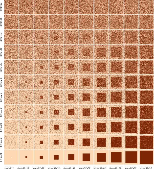
Figure 1: Images used in the single square setting. Noise level increases upward, whereas square size increases from left to right. At a glance, one can clearly see the squares in the center and lower images of the grid. The smaller the square, the faster it vanishes upward. This also happens when the square is too large, as the rim is confounded with the square.

Our object of study is a square image $\mathbf{x}$ of size $\sqrt{n}{\times}\sqrt{n}$ with $n$ pixels. The image $\mathbf{x}$ is binary: its elements $x_{ij}\in\{0,1\}$ for all $i,j$. The image is subject to noise, in the sense that the observed pixels of $\mathbf{x}$ are the result of an underlying, unobservable image whose pixels are flipped independently with an unknown probability $0<\delta<1$. Figure 1 illustrates the setting.

The task is to determine whether a square is present in the underlying unobserved image based on the noisy observation $\mathbf{x}$. Cast as a detection problem we have two hypothesis: if there is no square, the underlying image pixels are all $0$’s and the observed $1$’s are due to some of these $0$’s being flipped into $1$’s by noise; if a square of size $\sqrt{n_{1}}{\times}\sqrt{n_{1}}$ is indeed present, its unobserved pixels will have a value of $1$. If present, the size $n_{1}$ of the square as well as its position on the image are also unknown.

If the square is sufficiently large, we expect roughly $n_{1}(1-\delta)$ pixels to be $1$, and $n_{1}\delta$ pixels to be $0$. Correspondingly, the $n-n_{1}$ background pixels should consist of roughly $(n-n_{1})(1-\delta)$ $0$s and $(n-n_{1})\delta$ $1$s. If $\delta<0.5$, these two quantities should be distinguishable. Actually, if $\delta>0.5$ the same thing would happen, but the background would be darker than the foreground. Therefore, w.l.o.g., we consider error probabilities $0<\delta<0.5$ hereafter.

Note that a complete computer vision application usually includes two distinct stages: the first one produces a set of feasible candidates using some heuristic, and the second one validates the candidates, either jointly or separately, using some significance criterion. As we are interested in the latter problem, in this and all the following experiments, we assume the set of candidates to be fixed and given to us.

We will now work out the aforementioned detection problem using both frameworks.

5.1 MDL detection of a noisy square

In order to formulate the square detection problem under the MDL framework we consider the task of encoding the binary image $\mathbf{x}$ under two different hypothesis: the null hypothesis $H_{0}$, and the non-null hypothesis $H_{1}$. Each will result in a corresponding theoretical code-length: $L_{0}$ or $L_{1}$. The task now is to compute these values for the given image $\mathbf{x}$.

Under the null hypothesis, the unobserved image is all $0$s and the observed image is the result of some of these $0$s being flipped to $1$ independently and with unknown probability $\delta$. The observed image $\mathbf{x}$ is therefore an i.i.d. Bernoulli process $\mathbf{X}$ where $\mathbb{P}(X_{i}=1)=\delta$. One possible universal code for this case is the so-called Enumerative Coding [7]. This is a two parts code where the first part uses $\log n$ bits (if not specified, logarithms are in base $2$) to describe the number $k$ of ones in $\mathbf{x}$, and the second part gives the position of $\mathbf{x}$ within the lexicographical list of all sequences of length $n$ with $k$ ones; this requires $\log{n\choose k}$ bits:

(7) $$L_{0}=\log n+\log{n\choose k}.$$

In order to compute $L_{1}$, we assume that the unobserved image contains a single square of size $n_{1}=\sqrt{n_{1}}\times\sqrt{n_{1}}$ 1s whose upper-left corner is located at some arbitrary position $(i,j)$. The observed image $\mathbf{x}$ is the result of flipping those unobserved pixels independently with unknown probability $\delta$. Let $k_{1}$ be the number of 1s inside the square, $k_{0}=k-k_{1}$ the number of 1s outside the square, and $n_{0}=n-n_{1}$ the number of background pixels. Given this information, we treat both, background and square, as two independent Bernoulli sequences: the background with parameter $q_{0}=k_{0}/n_{0}$, and the square with parameter $q_{1}=k_{1}/n_{1}$. The resulting code-length is the concatenation of two codes, both analogous to $L_{0}$, plus $\log n$ bits for describing the location of the square, and $0.5\log n$ more bits to describe the square side:

(8) $$L_{1}=\frac{3}{2}\log n+\log n_{0}+\log{n_{0}\choose k_{0}}+\log n_{1}+\log{n_{1}\choose k_{1}}.$$

The hypothesis $H_{1}$ is selected when $L_{1}<L_{0}$. We can express this condition by defining the MDL score, $\mathrm{MDL}=L_{1}-L_{0}$,

(9) $$\mathrm{MDL}=\frac{3}{2}\log n+\log n_{0}+\log{n_{0}\choose k_{0}}+\log n_{1}+\log{n_{1}\choose k_{1}}-\log n-\log{n\choose k}.$$

A positive detection is declared when $\mathrm{MDL}<0$. As a final note, we remind the reader that this is not the only possible MDL formulation for this problem; just a reasonable one.

5.2 A-contrario detection of a noisy square

In the a-contrario framework, a test is defined for each possible structure to be detected or part evaluated; in our case each possible square in the image is a part and defines a test. Then, a random variable is associated to each test and an NFA is defined according to Definition 4.1. Using Proposition 4.2, $\mathrm{NFA}=N\,\mathbb{P}(\omega)$, where $N$ is the number of tests and $\mathbb{P}(\omega)$ is the probability of observing the event $\omega$ under the null hypothesis (usually called the background model). A detection is declared when the NFA value for a given event $\omega$ is below a certain threshold $\varepsilon$; the a-contrario setting ensures that the average number of false detections under $H_{0}$ is controlled by $\varepsilon$.

As for the number of tests $N$, there are two unknown quantities that determine each candidate structure in the current problem: the size of the square, $n_{1}$, and its location within the image, which can be specified by the linear index of the upper-left corner. For an $\sqrt{n}\times\sqrt{n}$ image we have $n$ possible positions and $\sqrt{n}$ possible values for $n_{1}$. This gives $N=n^{3/2}$ tests.

We assume the same null hypothesis $H_{0}$ as in the MDL formulation described before, i.e., the pixel values are independent Bernoulli random variables with probability $\delta$. The parameter $\delta$ is unknown, but can be estimated as the empirical density of $1$s in the image. Likewise, as before, we let $k$ be the total number of $1$s in the image, $n_{1}$ be the number of pixels inside the square, and $k_{1}$ be the number of 1s inside the square. Following the same notation, we set $q=k/n$, the fraction of 1s in the image.

In the notation of Section 4, each possible square in the image is a part $\mathbf{x}_{i}$ and the function $\xi$ count the number of pixels with value one in the square. According to the a-contrario approach, the region will be declared a detection if observing at least $k_{1}$ ones within the square is highly unlikely under the null hypothesis. We define the random variable $K_{1}$ corresponding to the number of 1s in the square under the null hypothesis $H_{0}$. We are interested in the event $\omega=\{K_{1}:K_{1}\geq k_{1}\}$. Given the empirical density estimation $q$, the probability of this event is,

$$\mathbb{P}[K_{1}\geq k_{1}]=\sum_{i=k_{1}}^{n_{1}}{n_{1}\choose i}q^{i}(1-q)^{n_{1}-i},$$

which is the tail of a Binomial distribution of parameters $n_{1}$ and $q$. We have now completed our calculation of the NFA:

(10) $$\mathrm{NFA}=n^{3/2}\sum_{i=k_{1}}^{n_{1}}{n_{1}\choose i}q^{i}(1-q)^{n_{1}-i}.$$

A square is detected when $\mathrm{NFA}\leq\varepsilon$. Again, this is not the only possible a-contrario formulation of this problem, but a reasonable one. Also, the modelling is similar to the previous MDL formulation for the same problem.

5.3 Comparison on a noisy square

At first sight, the criteria Eq. 9 and Eq. 10 seem quite unrelated. We will now develop further on these expressions and search for common ground from an analytical point of view.

We begin with Eq. 10, which is somewhat easier. The probability term above can be bounded from above using Hoeffding’s inequality [21],

(11) $$\mathbb{P}[K_{1}\geq k_{1}]\leq\left(\frac{q}{q_{1}}\right)^{n_{1}q_{1}}\left(\frac{1-q}{1-q_{1}}\right)^{n_{1}(1-q_{1})}\quad\text{for}\quad q_{1}>q.$$

(When $q_{1}\leq q$, it is easy to show that $\mathbb{P}[K_{1}\geq k_{1}]\geq\frac{1}{2}$ and it is not an interesting case.) We will use this upper-bound as an approximation to the probability term. Plugging this into Eq. 10 and expressing the result in logarithmic terms, we obtain:

(12) $$\log\mathrm{NFA}\approx\frac{3}{2}\log n+n_{1}q_{1}\log\frac{q}{q_{1}}+n_{1}(1-q_{1})\log\frac{1-q}{1-q_{1}}.$$

Taking $n_{1}$ as a common multiplier of the last two terms we get:

(13) $$\begin{split}\log\mathrm{NFA}&\approx\frac{3}{2}\log n+n_{1}\left[q_{1}\log\frac{q}{q_{1}}+(1-q_{1})\log\frac{1-q}{1-q_{1}}\right].\\ &=\frac{3}{2}\log n-n_{1}D(q_{1}||q),\end{split}$$

where $D(q_{1}||q)$ is the Kullback-Leibler divergence (KLD) of a Bernoulli distribution of parameter $q$ with respect to $q_{1}$. As expected, the more dissimilar $q_{1}$ is to $q$, the smaller the above term will be, and the more meaningful will be the square detection. If we choose the usual NFA parameter $\varepsilon=1$ we get a detection whenever

(14) $$\log{\mathrm{NFA}}\approx\frac{3}{2}\log n-n_{1}D(q_{1}||q)<0.$$

As the KLD is non-negative, the resulting score in Eq. 10 is guaranteed to result in a detection when $q_{1}$ is sufficiently distinguishable from $q$, the background model.

We will now work on Eq. 9. Using Stirling’s approximation for $\log{n\choose k}$ (see Appendix A) and rearranging terms we get,

(15) $$\begin{split}L_{0}&\approx\log n-\frac{1}{2}\log 2\pi+\frac{1}{2}\log\frac{n}{k(n-k)}+k\log\frac{n}{k}+(n-k)\log\frac{n}{n-k}\\ &=\log n-\frac{1}{2}\log 2\pi+\frac{1}{2}\log\frac{n}{k(n-k)}+n\left[-\frac{k}{n}\log\frac{k}{n}-\frac{n-k}{n}\log\frac{n-k}{n}\right]\\ &=\log n-\frac{1}{2}\log 2\pi+\frac{1}{2}\log\frac{n}{k(n-k)}+n\,h(q),\end{split}$$

where $h(q)=-q\log{q}-(1-q)\log(1-q)$ is the Binary Entropy function [6]. Similarly,

(16) $$\begin{split}L_{1}\approx\frac{3}{2}\log n&+\log n_{0}-\frac{1}{2}\log 2\pi+\frac{1}{2}\log\frac{n_{0}}{k_{0}(n_{0}-k_{0})}+n_{0}h(q_{0})\\ &+\log n_{1}-\frac{1}{2}\log 2\pi+\frac{1}{2}\log\frac{n_{1}}{k_{1}(n_{1}-k_{1})}+n_{1}h(q_{1}).\end{split}$$

Combining Eq. 15 and Eq. 16 we get the corresponding approximate expression for $\mathrm{MDL}$:

(17) $$\begin{split}\mathrm{MDL}\approx&\frac{3}{2}\log n+\log n_{0}+\log n_{1}-\log n+n_{0}h(q_{0})+n_{1}h(q_{1})-n\,h(q)\\ +&\frac{1}{2}\log\frac{n_{0}}{k_{0}(n_{0}-k_{0})}+\frac{1}{2}\log\frac{n_{1}}{k_{1}(n_{1}-k_{1})}-\frac{1}{2}\log\frac{n}{k(n-k)}-\frac{1}{2}\log 2\pi\\ =&\frac{3}{2}\log n+n_{0}h(q_{0})+n_{1}h(q_{1})-n\,h(q)\\ +&\frac{1}{2}\Big{[}g(k_{0},n_{0})+g(k_{1},n_{1})-g(k,n)\Big{]}-\frac{1}{2}\log 2\pi.\end{split}$$

where $g(k,n)=\log\frac{n^{3}}{k(n-k)}$. Observing that $q=\frac{n_{0}}{n}q_{0}+\frac{n_{1}}{n}q_{1}$, $n=n_{0}+n_{1}$ and $1=\frac{n_{0}}{n}+\frac{n_{1}}{n}$ allows us to write

(18) $$\begin{split}h(q)&=h\Big{(}\frac{n_{0}}{n}q_{0}+\frac{n_{1}}{n}q_{1}\Big{)}\\ &=-\left[\frac{n_{0}}{n}q_{0}+\frac{n_{1}}{n}q_{1}\right]\log q-\left[1-\frac{n_{0}}{n}q_{0}-\frac{n_{1}}{n}q_{1}\right]\log(1-q)\\ &=\frac{n_{0}}{n}\Big{[}-q_{0}\log q-(1-q_{0})\log(1-q)\Big{]}+\frac{n_{1}}{n}\Big{[}-q_{1}\log q-(1-q_{1})\log(1-q)\Big{]},\end{split}$$

and

(19) $$\begin{split}n_{0}h(q_{0})+n_{1}h(q_{1})-n\,h(q)=&n_{0}\Big{[}h(q_{0})+q_{0}\log q+(1-q_{0})\log(1-q)\Big{]}\\ +&n_{1}\Big{[}h(q_{1})+q_{1}\log q+(1-q_{1})\log(1-q)\Big{]}\\ =&-n_{0}D(q_{0}||q)-n_{1}D(q_{1}||q).\end{split}$$

Which leads us to:

(20) $$\begin{split}\mathrm{MDL}&\approx\frac{3}{2}\log n-n_{0}D(q_{0}||q)-n_{1}D(q_{1}||q)\\ &+\frac{1}{2}\Big{[}g(k_{0},n_{0})+g(k_{1},n_{1})-g(k,n)\Big{]}-\frac{1}{2}\log 2\pi.\end{split}$$

As with the a-contrario method, Eq. 20 is defined as long as $n,n_{0},n_{1},k_{0},k_{1}$ are all strictly positive. Let us repeat Eq. 14 here for reference:

$$\log{\mathrm{NFA}}\approx\frac{3}{2}\log n-n_{1}D(q_{1}||q).$$

As can be seen, both terms in the a-contrario expression are also present in the MDL one. The first one embodies the uncertainty in the parameters of the problem (the size of the image and the square). The second one measures the discrepancy between the empirical distribution of 1’s in the whole image (the null hypothesis) and the distribution of 1’s inside the square (the non-null hypothesis). The MDL expression adds a second KLD term which takes into account the difference between the distribution of 1’s in the image and its distribution outside the square; this reflects the fact that MDL takes both elements (object and background) into account when making a decision, whereas a-contrario concentrates on the object to be detected. Next, MDL includes a constant term $-(1/2)\log 2\pi$, (which can be disregarded for sufficiently large $n$). There is one last term which deserves some attention:

(21) $$\frac{1}{2}\Big{[}g(k_{0},n_{0})+g(k_{1},n_{1})-g(k,n)\Big{]}.$$

As shown in Appendix B, Eq. 21 this term can be bounded as:

(22) $$\log n\leq\frac{1}{2}\Big{[}g(k_{0},n_{0})+g(k_{1},n_{1})-g(k,n)\Big{]}\leq\log\frac{n^{\frac{5}{2}}}{4(n-2)}-1\approx\frac{3}{2}\log n-3.$$

In words, the above term accounts for an additional difference between MDL and a-contrario with a magnitude in the order of $\frac{3}{2}\log n$.

Figure 2 shows the result of a numerical experiment illustrating how the scores of both criteria vary as a function of the size of the square (horizontal axis) and the amount of noise (vertical axis). The results are quite similar up to the point where the area of the square is roughly half of the image (size $\approx 70$ as the image is $100\times 100$). In this first part, as the size of the square grows, the density is better evaluated and it is easier to distinguish $q_{1}$ from $q$; hence the detection is dominated by the term $D(q_{1}||q)$ in both formulations. The term $D(q_{0}||q)$ in MDL is negligible at first as the background covers almost all the image and $q_{0}\approx q$. The a-contrario formulation is a bit more sensitive than MDL; this is consistent with the extra term in MDL Eq. 21, which raises the detection threshold with respect to that of the one obtained with a-contrario.

For sizes larger than 71, the square encompass more than half of all the pixels. Thus, $q$ is more and more affected by $q_{1}$, and thus less distinguishable. The term $D(q_{1}||q)$ gradually vanishes and the a-contrario formulation is no longer able to detect the square. For MDL, on the other hand, as the square and the background have a symmetric role, the density $q_{0}$ becomes gradually distinguishable from $q$, and the term $D(q_{0}||q)$ becomes dominant. For the a-contrario approach, the square part is no longer anomalous while MDL, analysing the full data, still sees a difference.

In summary, the numerical experiments show that both MDL and a-contrario result in very similar detection criteria despite being strictly different from an analytical perspective.

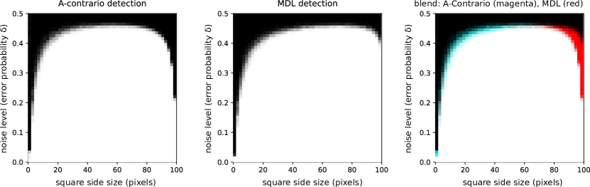
Figure 2: Single square detection using MDL and a-contrario for different square sizes (in terms of their side length) and noise level (expressed as probability $\delta$ of a pixel being flipped from 1 to 0 and vice-versa). For each noise level and square size the experiment was repeated for 100 different noise realizations. In the first two images, the intensity of each pixel corresponds to the percentage of cases where the corresponding method declared a detection (white: always, black: never). The last image is a color blend of the first two: the red channel corresponds to the MDL image, and green and blue channels (adding up to cyan) to a-contrario, so that white regions (blue plus red plus green) correspond to places where both methods yielded a detection).

6 Detection of multiple squares

In the previous section, we compared how the MDL and a-contrario approaches behave in a simple scenario involving a detection task; the goal of this section is to place both methods in a model selection problem.

In this case, instead of detecting the presence of individual squares, we will be dealing with many squares (see Fig. 3). All possible combinations of squares are considered and the task is to decide the number, size, and position of the squares that are deemed present.

Making the theoretically optimal decision according to both MDL and a-contrario usually requires the evaluation of a very large number of events. In practice, this is not possible and both criteria need to be applied to a much smaller subset of events using heuristics to propose relevant candidates. The real-life applications presented later in this work fall into this category: as the events involve the presence or absence of a large number of points or segments in all possible positions, orientations, etc., some heuristic is needed to narrow the choices. As the quality of these heuristics has an impact on the results, care must be taken in comparing MDL and a-contrario approaches under these circumstances. In this work, we sidestep this issue by using a common heuristic to define the candidates to be tested by both methods.

In the present case, considering all the possible squares, with all their possible sizes, even in a small image would result in a huge number of tests, and the problem would become practically intractable. For our purposes, it is enough to compare a reduced set of arrangements. Concretely, we generate a binary $256{\times}256$ image with a $2\times 2$ array of small squares separated by a given margin, which is a parameter. Note that the four small squares form a larger square whose size is always the same. As the margin grows, the size of the smaller squares becomes smaller. As before, the image is contaminated by independent Bernoulli noise with error probability $\delta$. Even in this case, there exist many possible explanations (each one of the small squares or combinations of 2, 3, or all of them). Without loss of generality, we reduce our candidate hypotheses to four: no detection, a single small square, four small squares, and the large square formed by considering all four small squares as a single one. We expect the choice to depend on the noise level and the proximity (margin) between the smaller squares.

6.1 MDL for multiple squares

The MDL detection scheme in this case is an extension of the procedure used for a single square. Each hypothesis consists of a number $c$ of squares, each one described exactly as we did before for one square (location, width, and pattern of $0$s and $1$s within), plus a background formed by the pixels which do not belong to any square, again described exactly as we did in the single square scenario (Equation 7).

The number of pixels in the image is $n$. The $i$-th square has $n_{i}$ pixels, $k_{i}$ of which are $1$. The number of background pixels is $n_{0}=n-\sum_{i=1}^{c}n_{i}$, and the number of those which are $1$ is $k_{0}=k-\sum_{i=1}^{c}k_{i}$. The corresponding empirical distributions are given by $q_{i}=k_{i}/n_{i},i=0,\ldots,c$.

The number of squares, $c$, is unknown beforehand, and so we must also describe it to the decoder. We can do this in a number of ways. A simple one that will usually do the work is an arbitrary geometric distribution, $P(c)\sim(1/2)2^{-c}$, so that the additional term is just $-\log P(c)=c+1$. Summing all, the expression for $L_{H}$ is:

$$L_{H}=\log n_{0}+\log{n_{0}\choose k_{0}}+\sum_{i=1}^{c}\left[(3/2)\log n+\log n_{i}+\log{n_{i}\choose k_{i}}\right]+c+1.$$

As before, the hypothesis with the smallest $L_{H}$ is chosen.

6.2 A-contrario for multiple squares

For the a-contrario formulation, we need to specify the family of tests, the background model, and the statistic used to evaluate a test. We use the same notation as before.

In this case, each test is determined by a set of squares defined inside the image domain. To take into consideration any number of squares, we can divide the family of tests according to the number of squares and allocate an accepted number of false alarms $\frac{\varepsilon}{2^{c}}$ to the sub-family of tests containing $c$ squares. We will set $\eta_{i}=2^{c}N(c)$, where $N(c)$ is the number of tests for $c$ squares. Since $\sum_{c}\frac{1}{2^{c}}=1$, we know that $\sum_{i}\frac{1}{\eta_{i}}=\sum_{c}\sum_{t\in N(c)}\frac{1}{2^{c}}\frac{1}{N(c)}\leq 1$; then, according to  Proposition 4.2, the quantity $\eta_{i}\,\mathbb{P}(K\geq k)$ is an NFA.

Let us count the number of test in the sub-family of $c$ squares. To simplify, we will neglect the squares overlapping and consider all possible ways of selecting $c$ squares in the image. Each square is determined by its upper-left corner pixel and side length. There are $n$ possible choices for the upper-left corner and $\sqrt{n}$ choices for the square side (this is an upper bound, as some of the squares considered are not really contained in the image domain). There are about $n^{\frac{3}{2}}$ possible squares in the image, and thus about $N(c)=\left(n^{\frac{3}{2}}\right)^{c}$ combinations of $c$ squares. Again, this is an upper bound; but the important thing is to get an estimation of the order of magnitude of the number of tests. All in all, $\eta_{i}=2^{c}\cdot n^{\frac{3}{2}c}$.

The background model $H_{0}$ considers that the pixels in the image are independent and follow a Bernoulli distribution. Its parameter $q$ is estimated as the empirical density: $q=\frac{k}{n}$.

To evaluate a candidate $s$ with $c$ squares, we sum the total number of 1s in all the squares $k(s)=\sum_{i\in s}k_{i}$ and the total number of pixels in all squares, $n(s)=\sum_{i\in c}n_{i}$. A candidate is considered a detection when the total number of $1$s in $s$ is too large to what would be expected according to the background model $H_{0}$. Assuming that the squares composing $s$ are not overlapping, then according to the background model $H_{0}$, the number of $1$s would be $K(s)$, a random variable following the binomial distribution of parameter $q$. Then, the probability of observing $k(s)$ in $H_{0}$ is:

$$\mathbb{P}(K(s)\geq k(s))=B\Big{(}n(s),k(s),q\Big{)}$$

where $B(n,k,q)$ is the tail of the binomial distribution:

$$B(n,k,q)=\sum_{i=k}^{n}{n\choose k}q^{i}(1-q)^{n-i}.$$

Finally, as $k(s)=\sum_{i}k_{i}$ and $n(s)=\sum_{i}n_{i}$, the NFA is:

$$\mathrm{NFA}=2^{c}\cdot n^{\frac{3}{2}c}\cdot B\left(\sum_{i}n_{i},\,\sum_{i}k_{i},\,\frac{k}{n}\right).$$

As usual, a detection is declared when $\mathrm{NFA}\leq\varepsilon$, with $\varepsilon=1$. As mentioned in Section 2, the $\mathrm{NFA}$ score can also be used to select the best configuration: the configuration with the smallest NFA is the least expected one under $H_{0}$ and is therefore the preferred one.

6.3 Comparison on multiple squares

In this case, the comparison will be limited to numerical experiments.

Sensitivity as a function of noise level

Fig. 3 shows the detection results of both MDL and a-contrario on the multiple squares case, for two different margin values (small and large), as the noise level increases.

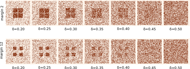
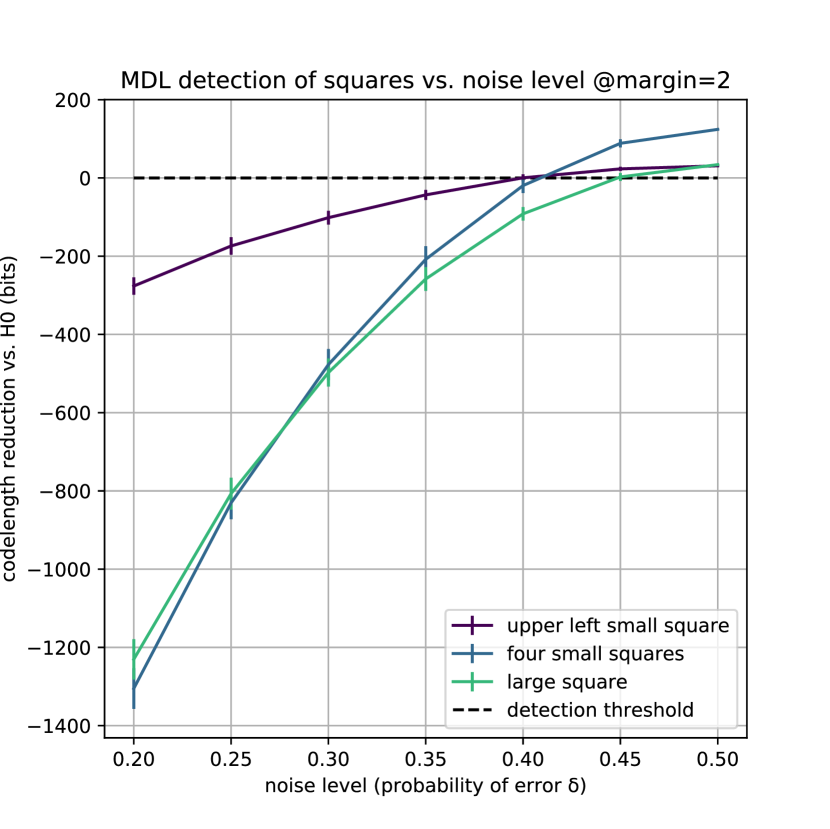
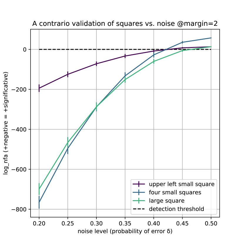
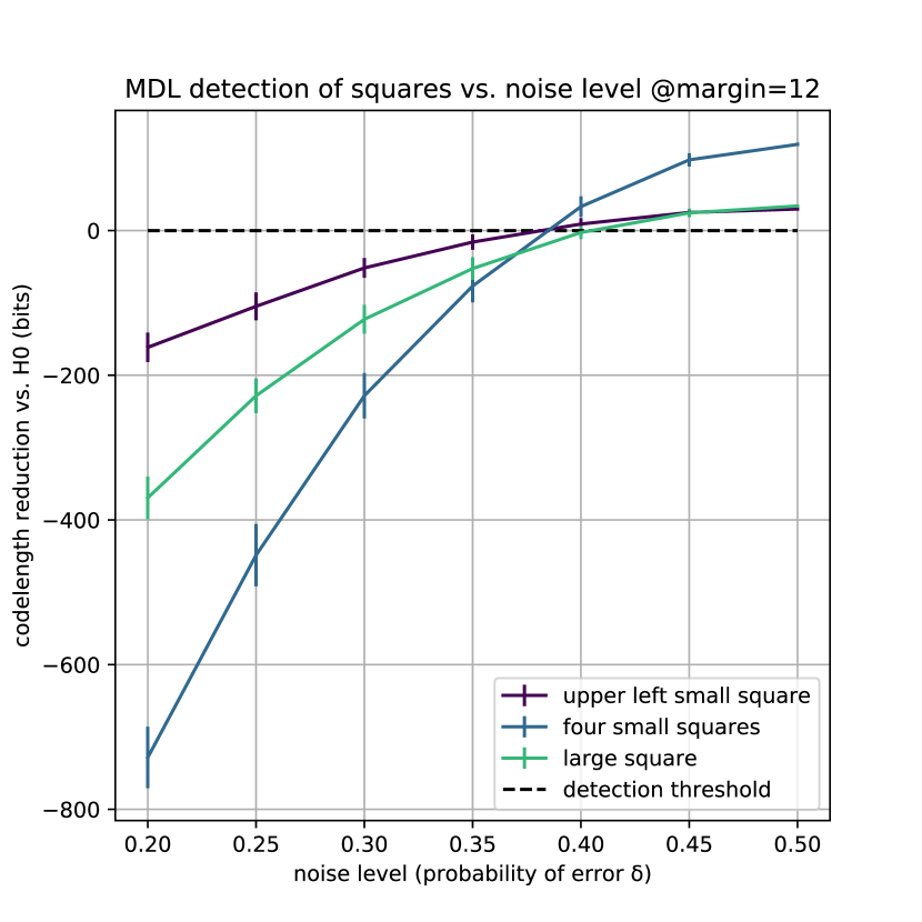
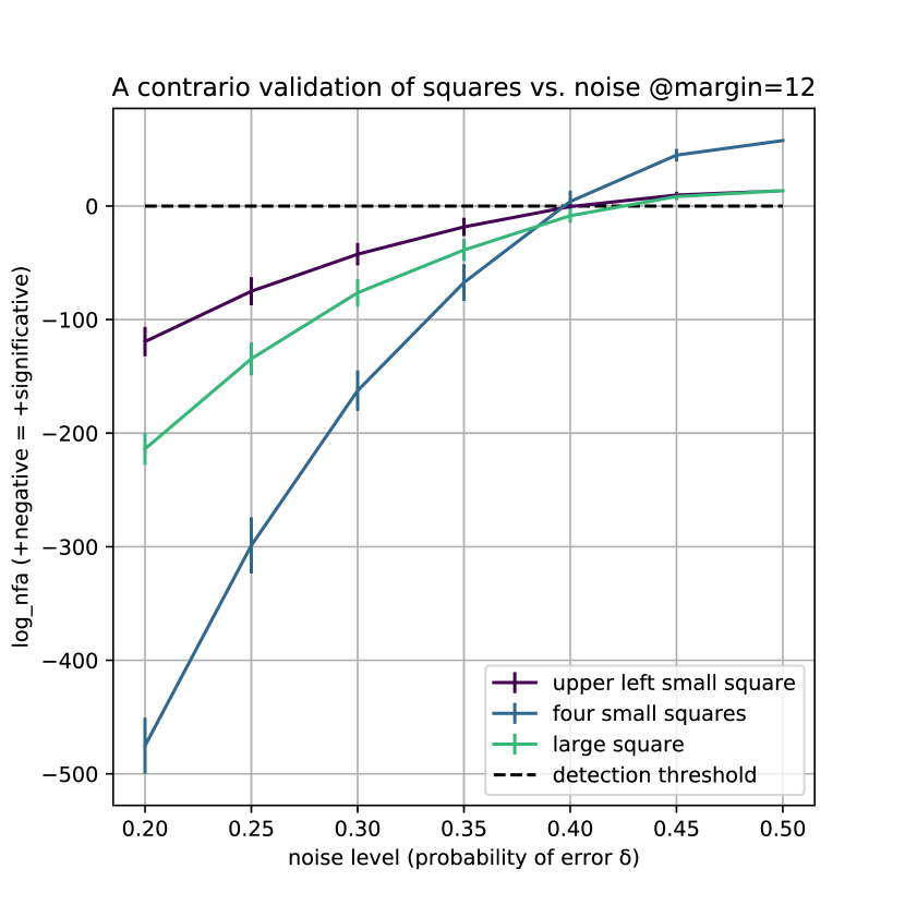
Figure 3: Detection of multiple squares as a function of the error probability, for fixed margins. First and second rows: sample images for this setting. Third row: MDL and a-contrario results for the small margin case; a detection occurs when the score is below $0$. Fourth row: results for the large margin scenario. In the a-contrario method, lower scores indicate more significant events. See the text for a discussion of these results.

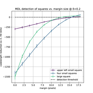
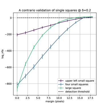
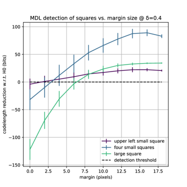
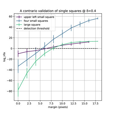
Figure 4: Detection of multiple squares as a function of the margin, for a fixed error rate $\delta$. The top row shows images of four squares separated by different margins under mild ($\delta=0.2$) noise. The second row shows similar images under high ($\delta=0.4$) noise. Third row shows the MDL (left) and a-contrario (right) results for $\delta=0.2$. A value below $0$ indicates a positive detection. Last row shows the experiment output for $\delta=0.4$. See text for a discussion.

For large margins, both methods produce the correct result (four small squares) up to a noise level of about $\delta=0.4$ (MDL actually stops detecting a little earlier, at about $\delta=0.38$). These thresholds correspond to the 5th image from the left of the second row of Fig. 3; after a visual inspection of those images, it can be argued that the automatic threshold of $\delta=0.4$ is in agreement with human perception.

For a smaller margin (2 pixels), again, both methods behave almost identically. Interestingly, both methods switch to the simpler model (large square) for noise levels $\delta\geq 0.3$; in this case, it is less clear which would be the reasonable limit with a casual inspection of the corresponding image (Fig. 3, first row, 3th image from the left).

Sensitivity as a function of margin size

Fig. 4 shows the results of both methods on the multiple squares experiment, this time while varying the size of the margin between the small squares. The experiment is repeated for low ($\delta=0.2$) and high ($\delta=0.4$) noise levels.

For the low noise setting, both methods give very similar results, with identical detection thresholds at a margin of size $16$; this corresponds to the next-to-last image on the first row of Fig. 4, which again seems to indicate that the results of both methods agree with the human perceptual threshold for this case.

In the (very) high noise setting, as can be seen in Fig. 4, it is clear that both methods switch to the simpler explanation of a single, large square, in all cases. Here a-contrario is again slightly more sensitive, detecting a square for a margin of up to $8$ pixels, whereas MDL stops doing so at a margin of $6$ pixels. The a-contrario threshold seems to be more in line with human visual perception in this case (Fig. 4). This could offer some sort of validation to the a-contrario method, which is inspired (to some extent) by the human visual system. We discuss this idea in a slightly more formal way in Section 10.

7 Approximation of shapes using polygons

In this experiment, we are presented with a closed curve that separates a foreground object from the background in a binary image. The curve is approximated by several connected dots defining a polygon, and the task is to simplify the polygonal approximation by removing unnecessary points. Ideally, we would like to select the optimal subset of vertices from all the possible subsets of initial points, but this quickly becomes computationally infeasible. This is a particular instance of the well-known, general problem of subset selection in statistics. As in the general case, one must resort to a manageable subset of candidate point subsets. Typically, two alternatives exist to construct those subsets: backward stepwise selection (BSS) and forward stepwise selection (FSS) (see [19, Chapter 3]).

In BSS, the starting subset $P^{0}$ is the full set of candidate points $P$. An initial fitness score $\phi^{0}$ is associated to $P^{0}$. Let $|A|$ denote the size or cardinality of the set $A$. At step $t$, $|P^{t}|$ candidate subsets are produced by removing each one of the $|P^{t}|$ points in $P^{t}$, and their corresponding scores are computed. If the score of the best candidate is smaller than $\phi^{t}$, then that candidate is declared to be the new best solution, $P^{t+1}$, and its score is assigned to $\phi^{t+1}$. The process stops at step $t$ if no candidate yields a score better than $\phi^{t}$, or $|P^{t}|=3$ (the smallest number of points in a non-degenerate polygon).

The FSS heuristic goes in the opposite direction: the general algorithm starts with an empty subset and greedily adds the best candidate in each iteration until the score $\phi^{t}$ can no longer be improved. In our case, the FSS algorithm would require us to begin with at least three points from $P$ (this can already be a problem if $P$ is large), and add points from $P$ until the addition of new points to $P^{t}$ does not improve the current score $\phi^{t}$.

Below we develop both a-contrario and MDL-guided BSS heuristics for choosing the best subset of points from the full polygon, which is obtained using the Devernay Sub-Pixel Edge Detector [16]. As the name suggests, this is a model selection problem, for which MDL is naturally suited. As before, we describe both approaches in detail and then proceed to compare their results on a number of selected cases.

7.1 MDL approach for polygon approximation

As before, we are presented with a 2D binary image $\mathbf{x}$ of $n$ pixels. The polygon is defined by an ordered set $P$ of $c$ vertex coordinates $(i,j)$. The interior of the polygon (which includes the vertices themselves) is denoted by $I$; the outside is defined by a set $O$. This problem is largely analogous to that of the single square problem presented in Section 5, the only difference being the description of the region itself, which is a polygon instead of a square. Thus, we follow the same general encoding strategy: for a given candidate polygon $P^{t}$ the code-length associated to it is $L(\mathbf{x},P^{t})=L(\mathbf{x}|P^{t})+L(P^{t})$. The first term is the concatenation of two enumerative codes: one for $I^{t}$, and one for $O^{t}$. Again, we define $n_{1}$ to be the number of pixels of the polygon in $I^{t}$, $k_{1}$ the number of 1s inside the polygon in $I^{t}$, $k_{0}=k-k_{1}$, and $n_{0}=n-n_{1}$. Note that $n_{0}$, $k_{0}$, $n_{1}$ and $k_{1}$ change for each iteration $I^{t}$ (to simplify the notation, the super-index $t$ was not added to $n_{0}$, $k_{0}$, etc). We get:

$$L(\mathbf{x}|P^{t})=\log n_{1}+\log{n_{1}\choose k_{1}}+\log n_{0}+\log{n_{0}\choose k_{0}}.$$

The interesting part is how to describe $P^{t}$, as there are different possibilities depending on various assumptions we may make about the polygon which could allow us to encode the coordinates in a clever way (e.g., differentially). As before, for the sake of simplicity, we will describe the 2D coordinates of $P^{t}$ as if they were independent. This requires $\log n$ bits per coordinate, so that $L(P^{t})=c\log n$. Finally, we also need to describe the number of vertices, $c$, which we do as we did in Section 6.1, requiring $c+1$ additional bits. The overall code-length is very similar to Eq. 8:

(23) $$L(\mathbf{x},P^{t})=1+c(1+\log n)+\log n_{1}+\log{n_{1}\choose k_{1}}+\log n_{0}+\log{n_{0}\choose k_{0}}.$$

Notice that the term $c+1$ was combined with $c\log n$ as $1+c(1+\log n)$, which also emphasizes that the cost of describing the number of vertices, $c+1$, is negligible for typical image sizes $n$ (e.g., $\log(256{\times}256)=16\gg 1$). The trade-off in Eq. 23 is simple: removing a vertex from $P^{t}$ will save us $1+\log n$ bits. On the other hand, this will introduce errors in the frontier between $I^{t}$ and $O^{t}$ so that the empirical distributions of $I^{t}$ and $O^{t}$ will deviate further from their true underlying Bernoulli distributions. A well-known result from Information Theory establishes that this will result in a longer overall code-length with overwhelming probability [6, Chapter 2].

7.2 A-contrario approach for polygon approximation

As with MDL, the a-contrario formulation for this case is mostly analogous to the square detection problem: given the foreground shape, the evaluation of its significance relies on the empirical density of its interior pixels. The main difference is that the family of tests includes all polygonal curves in the image domain instead of all squares.

As in the case of multiple squares, the set of tests is decomposed into subsets, each corresponding to a given number of sides in the polygon; the accepted number of false alarms for the subset of tests which consider polygons with $s$ sides is set to $2^{s}$. Now, given $s$, a crude approximation to the number of possible polygons with $s$ sides is to assume that any image pixel can be a vertex, which gives us $n^{s}$ possible polygons. Combining both factors, we obtain:

$$\eta_{s}=2^{s}\cdot n^{s}.$$

As before, $n_{1}$ is the number of pixels inside the polygon, $k$ the total number of 1s in the image, $k_{1}$ the number of 1s inside the polygon, and the empirical density is $q=\frac{k}{n}$. Under the null hypothesis, a Bernoulli process with $P(x=1)=q$, the probability of observing at least $k_{1}$ 1s among the total $n_{1}$ pixels inside the candidate polygon is given by

$$\mathbb{P}(K\geq k_{1})=B\left(n_{1},k_{1},q\right)$$

and the NFA is given by

$$\mathrm{NFA}=2^{s}\cdot n^{s}\cdot B\left(n_{1},\,k_{1},\,q\right).$$

When $\mathrm{NFA}<\varepsilon$ the event is considered $\varepsilon$-meaningful and the candidate is validated.

The NFA is by construction a quantity to decide the presence or not of a pattern. However, it can also be used to decide between alternative interpretations of the same data. When a given structure is indeed present in the data, a candidate similar to the actual structure, for example sharing most of the pixels, may also result in a meaningful test. Nevertheless, the actual structure would probably be the one with the largest deviation from the background model. This deviation from the background model is measured by the NFA. Thus, the candidate with the smallest NFA often corresponds to the actual structure. As a consequence, selecting the candidate with smallest NFA can be used as a model selection procedure.

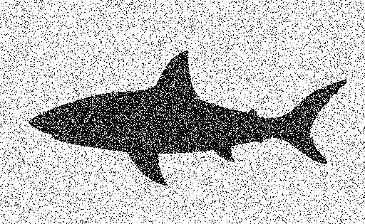
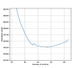
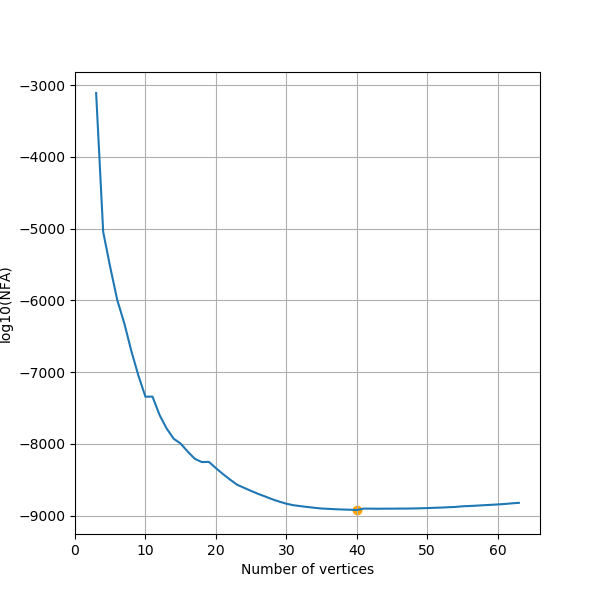
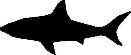
Figure 5: Polygon approximation comparison. Top left: noisy image; bottom left: full polygon estimated using the Devernay algorithm [12] (63 vertices); top center: MDL code-length vs. polygon size (the best is marked with a star); top right: $\log_{10}(\mathrm{NFA})$ vs. number of polygon vertices (the best is marked with a star); bottom center: best MDL polygon ($47$ vertices); bottom right: best a-contrario polygon ($40$ vertices).

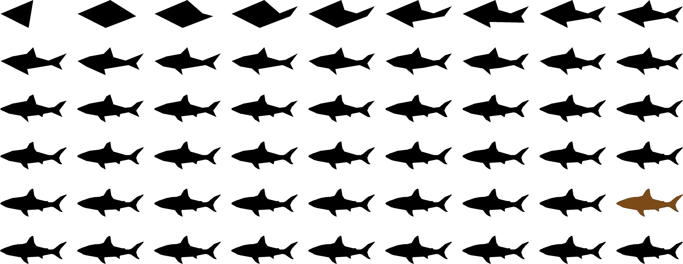
Figure 6: Sequence of candidate polygons obtained using BSS Selection guided by MDL. The polygon sizes range from $3$ to $56$. The chosen one is shown in gold ($47$ vertices).

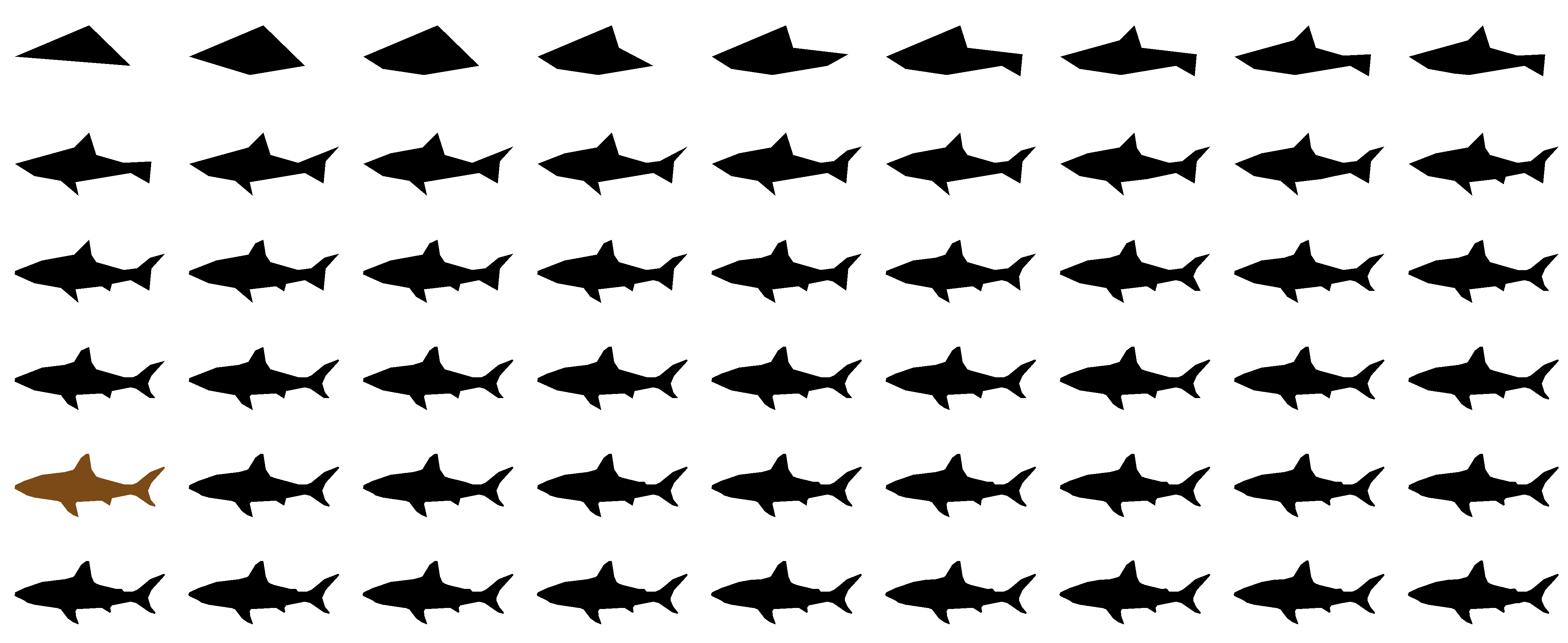
Figure 7: Sequence of candidate polygons obtained using BSS Selection guided by NFA value in the a-contrario approach. The polygon sizes range from $3$ to $66$. The chosen one is shown in gold ($40$ vertices).

7.3 Comparison on polygon approximation

Figure 5 illustrates the results obtained. Despite their differences, both methods produce similar results: the “score-vs-number of points” curves are similar in shape, the minima are close, and the approximated shapes are similar too. Figure 6 and Fig. 7 show the sequence of candidates obtained using the BSS heuristic guided by MDL and a-contrario respectively; comparing these figures, the differences between the BSS paths obtained using each method can be observed. Our aim is not to find which one has a “better” result (something difficult to define), but to show that both approaches can be used for a real model selection problem and that the solutions are similar.

8 Line segments in 2D images

The aim of this final task is to detect the solid line segments present in an image. The LSD algorithm [23, 15] is a popular and successful application of the a-contrario approach for this problem. Below we describe the original a-contrario-based LSD algorithm, develop its MDL counterpart, and compare the results of both algorithms on a number of examples.

LSD algorithm is based on the orientation of the image gradient. A fast heuristic is applied to group neighbor pixels which share a similar gradient orientation, producing a segmentation of the image into candidate regions. A rectangle is fit to each region, resulting in candidate line segments; these candidates are then evaluated independently using an NFA metric: those meaningful enough are kept, and the rest discarded. In order to apply MDL to this case, we need to formulate such detection sub-problem as a data compression one. Below we describe both approaches in detail, beginning with the original a-contrario method.

8.1 A-contrario line segment detection

Here we summarize the main ideas behind the LSD algorithm. We refer the reader to the original work [23] for further information, and to [15] for implementation details, in particular those pertaining to the heuristic search for candidates.

Given an initial image $\mathbf{x}$ with a total of $n$ pixels, the input to this method is an image gradient orientation map $\mathbf{d}\in[-\pi,\pi)^{n}$. The null hypothesis $H_{0}$ for this problem assumes that the gradient orientations are independent and isotropic, that is, $d_{ij}\sim\mathrm{Uni}([-\pi,\pi))\;\forall i,j.$

The family of tests is composed of all candidate rectangles in the image; a rectangle $r$ is the subset of image coordinates determined by the triad $(a,b,w)$, where $a$ and $b$ are the endpoints of the line segment that splits the rectangle in half along its shorter dimension (that is, the “center line” of the rectangle), and $w$ is the width of the rectangle, its shorter dimension. We also define $\lambda_{r}$ to be the normal direction of the segment $(a,b)$.

As with the other examples in this work, a heuristic is applied to produce a reduced set of feasible candidates to be tested for meaningfulness; the validation step is agnostic of this heuristic, assuming that all possible rectangles in the image, up to pixel precision, are tested.

For an image with $n$ pixels, the number of possible pairs of endpoints is bounded above by $n^{2}$, and the width of the rectangles by $\sqrt{n}$, yielding an upper bound for the number of tests of $N=n^{5/2}$. Despite its crudeness, using this approximation has proven good enough for practical purposes.

What remains is to define a criterion for deciding whether a particular candidate is declared as a positive detection, or discarded. There are many possible ways of doing so: below we describe the method used in [23, 15].

Given a candidate $r$, a positive detection is declared if the number of pixels in $r$ aligned with $r$ is too high to be produced by chance. A pixel $x_{ij}\in r$ is considered aligned if $|d_{ij}-\lambda_{r}|\leq\rho$ for some pre-defined tolerance $\rho\geq 0$.

Let $n_{r}=|r|$ be the number of pixels in $r$, and $0\leq k_{r}\leq n_{r}$ be the number of such pixels that are aligned. Following the a-contrario formalism, we define the NFA for this problem as

(24) $$\mathrm{NFA}(r)=N\cdot\mathbb{P}\Big{[}K_{r}\geq k_{r}\Big{]},$$

and declare a detection if $\mathrm{NFA}(r)\leq\varepsilon$. Here the random variable $K_{r}$ represents the number of aligned pixels in a rectangle $r$ for the null hypothesis $H_{0}$.

Under $H_{0}$, the gradient orientation map is assumed isotropic and the probability of a single pixel being aligned with $r$ is $\mathbb{P}(|d_{ij}-\lambda_{r}|\leq\rho)=\theta=\frac{\rho}{\pi}$. Furthermore, as the angles in $\mathbf{d}$ are assumed independent, the aforementioned events are themselves independent and $K_{r}$ is the sum of $n_{r}$ independent Bernoulli random variables. Thus, $K_{r}$ follows a Binomial distribution of parameter $\theta$,

(25) $$\mathbb{P}\Big{[}K_{r}\geq k_{r}\Big{]}=B\Big{(}n_{r},k_{r},\theta\Big{)}$$

where $B(n_{r},k_{r},\theta)$ is the tail of the binomial distribution. Note that, as expected,

$$\mathbb{P}\Big{[}K_{r}\geq k_{r}\Big{]}\rightarrow 0$$

as $k_{r}$ increases, which corresponds to increasingly more meaningful events.

To reduce the impact of the particular value used for the tolerance $\rho$, the LSD algorithm uses multiple values. Formally, each different value of $\rho$ defines a new test. If $\gamma$ is the number of different $\rho$ values used to evaluate each candidate, the grand total of tests must be corrected by this factor: $N=n^{5/2}\cdot\gamma.$

In summary, the NFA of a rectangle $r$ with $n_{r}$ pixels, $k_{r}$ of which are aligned, is given by:

(26) $$\mathrm{NFA}(r)=n^{5/2}\cdot\gamma\cdot B\Big{(}n_{r},k_{r},\theta\Big{)}.$$

As usual, we fix $\varepsilon=1$; all rectangles $r$ for which $\mathrm{NFA}(r)<1$ are considered detections.

8.2 MDL line segment detection

The object on which the line segment detection is performed in LSD is not the original image $\mathbf{x}$ itself, but its gradient orientation map $\mathbf{d}$. In order to apply the MDL criterion to this problem, it is this data that we shall encode. Furthermore, in LSD, the NFA criterion is applied independently to a set of candidate rectangles based only on the values of $\mathbf{d}$ and the normal of the rectangle $r$, $\lambda_{r}$. Accordingly, in order to produce a meaningful comparison between both criteria, we shall apply MDL to the problem of compressing $\mathbf{d}$ within each candidate rectangle $r$.

The modular design of the public LSD implementation [15] allows us to quickly test the proposed MDL variant by simply replacing the NFA criterion with the MDL one. This also provides a common set of candidates to work with, so that the results are easier to analyze and compare solely in terms of the criteria themselves.

The encoding problem for this case is as follows. We need to describe the gradient orientation map $\mathbf{d}$. According to the LSD pipeline, each element of $\mathbf{d}$ can be computed as a function of three pixels from $\mathbf{x}$, each taking on $2^{8}$ possible values. Correspondingly, each $\mathbf{d}_{ij}$ can take on $2^{24}$ possible values.

We are already given a set of candidate rectangles which may contain a significant portion of points aligned with their respective normal directions $\lambda$. As with LSD, we declare a point $(i,j)$ to be aligned with its corresponding rectangle if $|d_{ij}-\lambda_{r}|\leq\rho$, where $\rho$ is a threshold to be defined. The points that do not belong to any rectangle are ignored and are assumed to be described using an uniform distribution on the $2^{24}$ possible angle values.

Let $n_{r}$ be the number of points in a rectangle $r$ and $\mathbf{d}_{r}$ be the subset of elements of $\mathbf{d}$ indexed by the coordinates in $r$. In the MDL paradigm, a rectangle $r$ will be declared detected if we obtain a shorter description length by assuming them to belong to the rectangle $r$, rather than to the background. Formally, let $L(\mathbf{d}_{r},r)$ be the description length obtained if we assume that the points in $r$ form a line segment, and $L(\mathbf{d}_{r},H_{0})$ be the one obtained if they are assumed to be background pixels. Note that, under the uniform assumption, the latter is simply $L(\mathbf{d}_{r},H_{0})=24n_{r}.$

For $L(\mathbf{d}_{r},r)$, as before, we have to consider two pieces of information: the description of the rectangle itself, $L(r)$, and the description of the aligned points given $r$, $L(\mathbf{d}_{r}|r)$. The simplest description of $r$, although somewhat wasteful, is to describe its two endpoints and its width. Each endpoint requires $\log n$ bits. As in LSD, we bound the width by $\sqrt{n}$. This gives us a total of $\frac{5}{2}\log n$ bits per rectangle, which is the number of tests $N$ in the a-contrario framework (before the correction factor $\gamma$ applied due to the different angle thresholds).

A rectangle contains aligned points, unaligned points, and points whose gradient is considered undefined by the gradient computation algorithm. Our strategy is to encode the aligned points with one distribution, and the unaligned and undefined points with another. In order to describe the subset of aligned points we resort once again to an Enumerative Code as the one used in Section 5 and Section 6. If $n_{r}$ is the total number of points in the rectangle and $k_{r}$ is the number of those that are aligned, we require $\log n_{r}+\log{n_{r}\choose k_{r}}$ bits to indicate which of them are so. The unaligned/undefined points are described as background samples using $24$ bits each, for a total of $[n_{r}-k_{r}]24$ bits.

As for the aligned points, we know that $|d_{ij}-\lambda_{r}|\leq\rho$. A simple and conservative hypothesis in this case is that the angles $d_{ij}\sim\mathrm{Uni}[\lambda_{r}-\rho,\,\lambda_{r}+\rho]$. Now, as the $2^{24}$ possible angles are approximately uniformly distributed on $[-\pi,\pi]$, we expect about $(\rho/\pi)2^{24}$ possible values to fall within $[\lambda_{r}-\rho,\,\lambda_{r}+\rho]$.

In summary, for a rectangle $r$ with $n_{r}$ points, $k_{r}$ of which are aligned, we obtain:

$$L(\mathbf{d}_{r},r)=\frac{5}{2}\log n+\log n_{r}+\log{n_{r}\choose k_{r}}+24(n_{r}-k_{r})+(24+\log\rho/\pi)k_{r}.$$

Noting that $24(n_{r}-k_{r})+(24+\log\rho/\pi)k_{r}=24n_{r}+k_{r}\log\rho/\pi$, the MDL score is given by:

(27) $$L(\mathbf{d}_{r},r)-L(\mathbf{d}_{r},H_{0})=\frac{5}{2}\log n+\log n_{r}+\log{n_{r}\choose k_{r}}+k_{r}\log(\rho/\pi).$$

As $\rho<\pi$, the last term, which represents the reduction in code-length due to the tighter distribution of the aligned samples, is strictly negative. The other terms, all related to the description of the rectangle, are all non-negative. Thus, intuitively, the decision rule of Eq. 27 will deem a rectangle significant if enough points $k_{r}$ are aligned so that the savings outweight the cost of describing the rectangle. Note also that the term $\log{n_{r}\choose k_{r}}$ is positive but diminishes with $k_{r}$ (and becomes $0$ when $k_{r}=n_{r}$, that is, all points are aligned), reinforcing the evidence of alignment as $k_{r}$ grows.

As a final comment, notice that we have not added a term for the number of segments in the image. This is because, contrary to the previous examples, we are considering the detection of each segment as an independent test, instead of considering the set of segments in the image as a whole. In terms to be explained in Section 9, it work by parts.

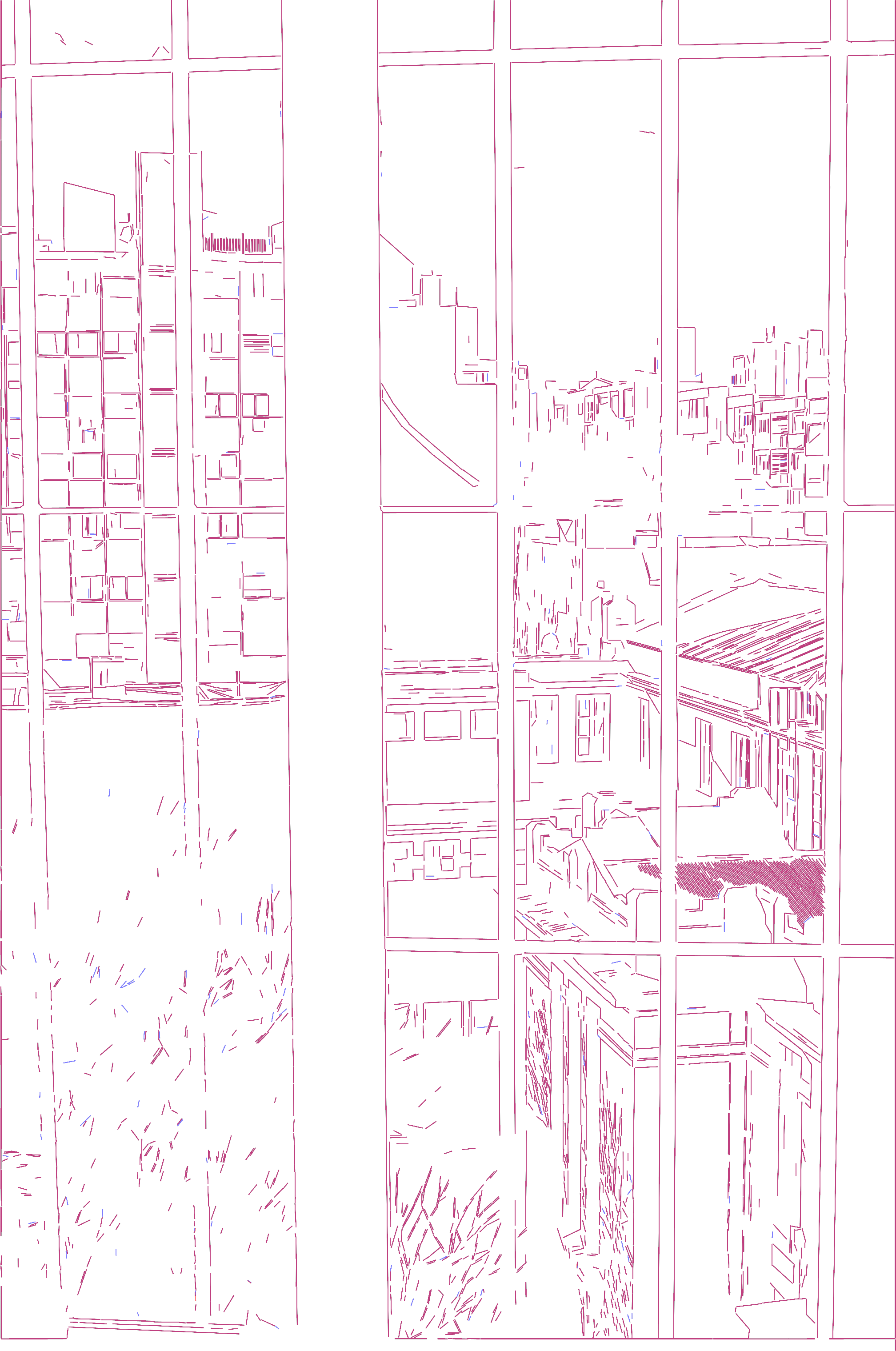
Figure 8: Visual comparison of line segments detected using a-contrario (blue) and MDL (red) approaches; segments detected by both are shown in violet. As can be observed, both methods yield extremely similar results (this is a high resolution image; zoom in to see details).

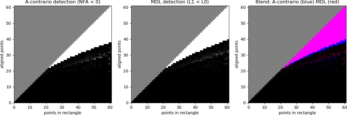
Figure 9: Line Segment Detection probability as a function of the number of points within a candidate rectangle, and the number of those points which are aligned. The size of the rectangle is cut at $60$ (the largest value for which we have samples along the whole vertical axis), and of course the number of aligned points cannot exceed the size of the rectangle (this region is filled with gray in all three images). Again both criteria produce very similar results.

8.3 Comparison on line segment detection

Here, as in the polygon approximation case (Section 7), our aim is to show that it is possible to use both approaches for a real detection problem and that the solutions are similar. Figure 8 shows a visual comparison of both detection criteria on a sample image. Line segments detected using a-contrario are marked in blue and the ones detected by MDL in red. Segments which were detected by both are shown in violet. As can be seen, both methods yield extremely similar results.

In order to analyze the detection capability of both methods we plot the probability of detection for different combinations of rectangle size and number of aligned points on a large number of test images. Fig. 9 compares the results of both approaches on the Line Segment Detection problem. The figures show the probability of detection as a function of the number of points within a candidate rectangle, and the number of those points which are aligned. The size of the rectangle is cut at $60$ (this is the largest value for which we have samples along the whole vertical axis), and of course the number of aligned points cannot exceed the size of the rectangle. The white region correspond to the detections in each case. For example, both methods detect a segment when there are at least 30 aligned points in a rectangle with 40 points, and naturally there is a limit of 40 aligned points in that case. The 3rd figure is a comparison between the results of both methods. It can be seen that again both criteria produce very similar results and the a-contrario approach is a bit more sensitive, i.e. produce detections with a lower number of aligned points in the rectangle.

9 When are MDL and a-contrario equivalent?

We have shown various examples where MDL and a-contrario lead to similar formulations and very similar numerical results. Nevertheless the formulations are strictly different. Indeed, MDL and a-contrario are in general different theories. In this section we present some conditions under which MDL and a-contrario approaches result in exactly the same criterion.

As we observed before, MDL implies selecting among a family of possible descriptions, the one with the shortest description of the whole data. On the other hand, the a-contrario approach concentrates on detecting parts of the data with anomalous statistics. This is a key observation, pointing to an important difference and also suggesting how to connect the two approaches. The connection can be obtained by forcing MDL to work also by parts. As we will see, given an a-contrario modeling, it is possible to build a MDL modeling resulting in exactly the same decision. The opposite is not true; MDL is a more general theory.

Following the description in Section 4, let $\mathbf{x}$ be a data vector taking values in a finite alphabet $\mathcal{X}$ and let $\{\mathbf{x}_{1},\,\mathbf{x}_{2},\ldots,\mathbf{x}_{N}\}$ be a family of $N$ parts. The ordering function $\xi$ acts on data vectors $\mathbf{x}_{i}\in\mathcal{X}^{n_{i}}$ and produces real numbers $y_{i}=\xi(\mathbf{x}_{i})$. Finally, a stochastic model $H_{0}$ is required for background data; here we can follow Laplace’s principle of indifference and assume that all the elements in $\mathcal{X}^{n}$ are equally probable under $H_{0}$. A part $\mathbf{x}_{i}$ will be considered anomalous when observing a value $y_{i}=\xi(\mathbf{x}_{i})$ or larger is a rare event under $H_{0}$. To be precise, an anomaly is declared when

(28) $$N\cdot\mathbb{P}[Y_{i}\geq y_{i}]\leq\varepsilon,$$

where $Y_{i}$ is a random variable corresponding to $y_{i}$ under $H_{0}$. Then, by Proposition 4.2, the expected number of false alarms in $H_{0}$ is bounded by $\varepsilon$. As a consequence, $\varepsilon$ determines the mean number of false alarms we are ready to accept per data set $\mathbf{x}$.

With these elements, we can now specify the equivalent MDL modeling. Three assumptions are required:

1. The vector $\mathbf{x}$ is coded as random data (the background), with the exception of some selected parts; those parts are selected from a family of $N$ and will be handled independently from each other.

2. In each potential part $\mathbf{x}_{i}$, the configurations with larger $\xi(\mathbf{x}_{i})$ should be favoured.

3. In each part $\mathbf{x}_{i}$, the configurations to be coded differently than the background must use the same code-length $l_{i}$.

Under these assumptions, to decide whether a given part should be described differently than the background or not, both lengths must be compared. When treated as background, the code-length for the part is $\log|\mathcal{X}^{n_{i}}|$. On the other hand, when described as a particular part, we need to specify which part is going to be described: this requires $\log N$ bits. Then, we need to specify the configuration of $\mathbf{x}_{i}$: this requires $l_{i}$ bits. Notice that the part needs not to be specified when coded as background as all the elements of $\mathbf{x}$ not included in a particular part will be coded as background; only the parts to be coded differently must be specified, and the rest is background. Thus, $\mathbf{x}_{i}$ will be described as a particular part when

(29) $$\log N+l_{i}<\log|\mathcal{X}^{n_{i}}|.$$

In other words, this makes sense when

$$l_{i}<\log|\mathcal{X}^{n_{i}}|-\log N,$$

which means that at most $\frac{|\mathcal{X}^{n_{i}}|}{N}$ configurations of $\mathbf{x}_{i}$ can be coded in that particular way. Which configurations? The ones with the largest $\xi(\mathbf{x}_{i})$ values. When the following condition

$$\Big{|}\big{\{}v\in\mathcal{X}^{n_{i}},\,\,\xi(v)\geq\xi(\mathbf{x}_{i})\big{\}}\Big{|}<\frac{|\mathcal{X}^{n_{i}}|}{N}$$

is satisfied, this implies that $\mathbf{x}_{i}$ is among the $\frac{|\mathcal{X}^{n_{i}}|}{N}$ configuration with largest $\xi(\mathbf{x}_{i})$ and should be coded as a especial part. This in turn is equivalent to

$$N\frac{\Big{|}\big{\{}v\in\mathcal{X}^{n_{i}},\,\,\xi(v)\geq\xi(\mathbf{x}_{i})\big{\}}\Big{|}}{|\mathcal{X}^{n_{i}}|}<1,$$

which is equivalent to

$$N\cdot\mathbb{P}\big{[}\xi(\mathbf{X}_{i})\geq\xi(\mathbf{x}_{i})\big{]}<1,$$

where $\mathbf{X}_{i}$ is a random vector following $H_{0}$. This condition is equivalent to Eq. 28 when setting $\varepsilon=1$ and the same a-contrario criterion is obtained.

Notice that the same can be done when a non-uniform risk distribution $\eta_{i}$ is used. Indeed, the condition $\sum_{i=1}^{N}\frac{1}{\eta_{i}}\leq 1$ makes that $\log\eta_{i}$ satisfy the Kraft inequality and thus there is a prefix coding for the parts with code-lengths $\log\eta_{i}$. Using $\log\eta_{i}$ instead of $\log N$ in Eq. 29 leads to the condition

$$\eta_{i}\cdot\mathbb{P}\big{[}\xi(\mathbf{X}_{i})\geq\xi(\mathbf{x}_{i})\big{]}<1,$$

which again is the a-contrario criterion when setting $\varepsilon=1$.

From the MDL point of view, the a-contrario approach can be thought as a particular strategy for modelling. In the context of the MDL framework, this strategy is often sub-optimal. Nevertheless, the complexity of an optimal modeling imposes very often in practice a sub-optimal approach in MDL applications. To prevent a combinatorial explosion, the modeling is often done by independent parts (as was the case, for example, in Section 8.2).

The conditions required for the equivalence are not exactly satisfied in the examples described in this work, only approximately in some of the cases. As a consequence, the criteria obtained are only similar but not equivalent.

10 Discussion

The MDL principle and the a-contrario approaches are very different theories, in their philosophical and mathematical foundations. Nevertheless, both share similar characteristics. Both can be used in model selection problems and in detection problems. Both require a modeling step and a given problem can be modeled in various ways. Tradition favors some kinds of models in MDL and other kinds in a-contrario. Here we made an effort to handle the same problems by both approaches and enforce the modeling to be similar. As expected, the resulting criteria are different; surprisingly the resulting decisions are however very similar. This may be explained by Kolmogorov’s definition of randomness, as suggested in the introduction. Indeed, there is a connection between the compression resulting from a model and the non-accidentalness evaluated by the same model. Thus, a configuration considered as accidental in the a-contrario approach will not lead to a shorter description than the random model in MDL, leading to similar decisions. Nevertheless, this conclusion is only valid when the same (or similar) modeling is used; otherwise, a richer family of models could handle more complex patterns, allowing for a shorter description or identifying a non-accidental configuration.

Making the theoretically optimal decision according to both, MDL and a-contrario usually require the evaluation of a very large number of events. In practice, this is not possible and both criteria need to be applied to a much smaller subset of events using heuristics to propose relevant candidates. The real-life applications presented in this work fall into this category, as the events involve the presence or absence of a large number of points or segments in all possible configurations; a heuristic such as BSS or FSS is thus needed.

In the MDL formulation, the detection or model selection is determined by the modeling step (and the required heuristics in most cases). The a-contrario approach requires, in addition, setting the expected number of false alarms threshold $\varepsilon$. This is a clear advantage of the MDL approach as it requires one less parameter to be set (except in some particular cases where the ability to specify the false detection rate may be useful). Nevertheless, considering that the a-contrario formulation already includes the number of tests performed, the reasonable range of values for $\varepsilon$ is quite limited. Moreover, given the usual logarithmic dependence on $\varepsilon$, the actual impact of this parameter is very limited. Indeed, the frontier between a pattern that can be observed by accident or not is usually very sharp. This is confirmed in our experiments where $\varepsilon$ was always set to one, and in all cases, MDL and a-contrario resulted in very similar criteria.

A key limitation of MDL is in dealing with real-valued data. As the performance of a model is measured by how much it can compress the data, any reasonable model has to be able to produce a code length that is significantly shorter than the “raw” description of the data. For example, if we have a one megapixel 8-bit image, any description over 8 megabits should be discarded. This is already a problem with MDL on signals over large alphabets but becomes virtually impossible if the data is real-valued, simply because describing real numbers requires infinite precision. Quantization is therefore a mandatory step, and optimum quantization is still an open problem in Information Theory. On the other hand, real numbers are not a problem in the a-contrario framework as long as the events to be detected can be cast as thresholds on appropriate random variables.

Several works discuss the connection between the parsimony principle and the likelihood principle [18, 5, 32]. Similarly, the present work draws the connections between the parsimony principle and the non-accidentalness principle as expressed in the MDL and a-contrario formalisms.

A key difference is that the MDL principle focuses on the best interpretation for the whole data while the a-contrario approach concentrates on parts of the data with anomalous statistics. To prevent a combinatorial explosion, in practice MDL is often dictated to evaluate the data by parts. Again, the theoretical differences vanish in real applications. The examples presented in this work and the conditions of equivalence in Section 9 suggest that when working by parts, both MDL and a-contrario share a common ground. More generally, any departure from randomness should allow for a shorter description in MDL using an appropriate modelling; the same departure from randomness should be detected as an anomaly by an appropriate a-contrario modelling. In a sense, both approaches embrace a common rationale which may be described with the words of Dennett: “Any nonrandomness in the flux [of energy striking one’s sensory organs] is a real pattern that is potentially useful information for some possible creature or agent to exploit in anticipating the future.” [9, p.128]

11 Conclusion

MDL and a-contrario are seemingly very different approaches, typically used in different scenarios. The former try to codify the whole data and the later concentrates on the detection of some anomalous structures. After having compared both criteria, under different settings, both analytically and in practice, we have found that they are, in fact, closely related. Our initial discussion makes it clear that both methods share a common root in the Algorithmic Complexity theory. An in-depth analysis of both methods in toy examples has shown that there are significant connections in the tools and the mathematical formulations behind the metrics used (code-length and NFA). When applied, we found that both methods yield similar results in all the scenarios studied; in some cases, the results are almost identical. Last but not least, we have also shown that both MDL and a-contrario methodologies can be used interchangeably for detection (single hypothesis) and model selection (multiple hypotheses) scenarios, without significant theoretical or practical complications.

Having established these connections opens up new and exciting lines of work involving the cross-dissemination of these methods to new domains. Examples of these are the application of MDL tools for Computer Vision problems or using the a-contrario formalism for tackling a wide range of model selection problems in and outside the fields of Computer Vision and Image Processing.

Appendix A Stirling’s approximation for binomial terms

Here we develop the Stirling approximation of ${n\choose k}$. First, we have the basic Stirling approximation for $n!$:

$$n!\approx\sqrt{2\pi n}e^{-n}n^{n}.$$

When plugged into ${n\choose k}=\frac{n!}{k!(n-k)!}$ we obtain:

$$\frac{n!}{k!(n-k)!} \approx\frac{\sqrt{2\pi n}e^{-n}n^{n}}{\sqrt{2\pi k}e^{-k}k^{k}\sqrt{2\pi(n-k)}e^{-(n-k)}(n-k)^{n-k}}$$

$$=\frac{1}{\sqrt{2\pi}}\sqrt{\frac{n}{k(n-k)}}\frac{n^{n}}{k^{k}(n-k)^{n-k}}$$

$$=\frac{1}{\sqrt{2\pi}}\sqrt{\frac{n}{k(n-k)}}\left(\frac{n}{k}\right)^{k}\left(\frac{n}{n-k}\right)^{n-k}$$

Taking logarithms, we arrive at:

$$\log{n\choose k}\approx\frac{1}{2}\log\frac{1}{2\pi}+\frac{1}{2}\log\frac{n}{k(n-k)}+k\log\frac{n}{k}+(n-k)\log\frac{n}{n-k}.$$

Appendix B Bounds on g(k,n)

Recall that $g(k,n)=\log\frac{n^{3}}{k(n-k)}$, which is a convex function of $(k,n)$. Thus, the terms $g(k_{0},n_{0})+g(k_{1},n_{1})$ form a convex function on $(k_{0},n_{0},k_{1},n_{1})$ which is block-symmetric in $(k_{0},n_{0})$ and $(k_{1},n_{1})$ as both are interchangeable. Since the restrictions in place establish that $k_{0}+k_{1}=k$ and $n_{0}+n_{1}=n$, the minimum is attained at the mid-point $(k_{0},n_{0})=(k_{1},n_{1})=(k/2,n/2)$. Thus, for fixed $k$,$n$, we have $g(k/2,n/2)=\log\frac{n^{3}/2}{k(n-k)}=g(k,n)-1$. Thus,

$$\begin{array}[]{cl}\min_{k_{0},n_{0},k_{1},n_{1}}&g(k_{0},n_{0})+g(k_{1},n_{1})\\ s.t.&k_{0}+k_{1}=k,n_{0}+n_{1}=k\end{array}=2g(k,n)-2$$

and

$$\frac{1}{2}\Big{[}g(k_{0},n_{0})+g(k_{1},n_{1})-g(k,n)\Big{]}\geq\frac{1}{2}[2g(k,n)-2-g(k,n)]=\frac{1}{2}g(k,n)-1.$$

Now, $g(k,n)$ is minimized when $k=n/2$ with $g(\frac{n}{2},n)=2+\log n$. Thus we have a lower bound (which is tight when $n$ is a multiple of $4$):

(30) $$\frac{1}{2}\Big{[}g(k_{0},n_{0})+g(k_{1},n_{1})-g(k,n)\Big{]}\geq\frac{1}{2}\log n.$$

The upper bound can be worked in a similar way. Since, for fixed $n$, $g(k,n)$ is symmetric and strictly convex around $k=n/2$, we know that the maxima occur at the extreme points of the feasible set, $1\leq k\leq n-1$. Thus, $\max_{k}g(k,n)=g(1,n)=g(n-1,n)=\log\frac{n^{3}}{n-1}$. Applying analogous arguments as before, the maxima of the symmetric function $g(k_{0},n_{0})+g(k_{1},n_{1})$ must occur when $n_{1}=n_{0}=n/2$ and $k_{0}=k_{1}=1$ so that

$$\begin{array}[]{cl}\max_{k_{0},n_{0},k_{1},n_{1}}&g(k_{0},n_{0})+g(k_{1},n_{1})\\ s.t.&k_{0}+k_{1}=k,\,\,n_{0}+n_{1}=n\end{array}=2\log\frac{n^{3}}{4(n-2)}.$$

Recalling that $g(k,n)$ is minimized by $g(\frac{n}{2},n)=2+\log n$, we can now maximize the whole term over $2\leq k\leq n-2$ and obtain its upper bound:

$$\frac{1}{2}\Big{[}g(k_{0},n_{0})+g(k_{1},n_{1})-g(k,n)\Big{]}\leq\frac{2}{2}\log\frac{n^{3}}{4(n-2)}-\frac{1}{2}(2+\log n)=\log\frac{n^{\frac{5}{2}}}{4(n-2)}-1.$$

The remaining MDL term Eq. 21 has now been bounded as follows:

(31) $$\log n\leq\frac{1}{2}\Big{[}g(k_{0},n_{0})+g(k_{1},n_{1})-g(k,n)\Big{]}\leq\log\frac{n^{\frac{5}{2}}}{4(n-2)}-1\approx\frac{3}{2}\log n-3.$$

References

- [1] M. K. Albert and D. D. Hoffman, Genericity in spatial vision, in Geometric Representations of Perceptual Phenomena: Articles in Honor of Tarow Indow’s 70th Birthday, D. Luce, K. Romney, D. Hoffman, and D’Zmura M., eds., Erlbaum, 1995, pp. 95–112.
- [2] A. Barron, J. Rissanen, and B. Yu, The minimum description length principle in coding and modeling, IEEE Trans. IT, 44 (1998), pp. 2743–2760.
- [3] G. J. Chaitin, On the simplicity and speed of programs for computing infinite sets of natural numbers, Journal of the ACM, 16 (1969), pp. 407–422.
- [4] G. J. Chaitin, Algorithmic information theory, IBM Journal of Research and Development, 21 (1977), pp. 350–359.
- [5] N. Chater, Reconciling simplicity and likelihood principles in perceptual organization, Psychological Review, 103 (1996), pp. 566–581.
- [6] T. Cover and J. Thomas, Elements of information theory, John Wiley and Sons, Inc., 2 ed., 2006.
- [7] T. M. Cover, Enumerative source encoding, IEEE Trans. IT, 19 (1973), pp. 73–77.
- [8] T. M. Cover and J. A. Thomas, Elements of information theory, John Wiley and Sons, Inc., 1991, /bib/private/cover/Wiley.Interscience.Elements.of.Information.Theory.Jul.2006.eBook-DDU.pdf.
- [9] D. C. Dennett, From Bacteria to Bach and Back, W. W. Norton & Company, 2017.
- [10] A. Desolneux, L. Moisan, and J.-M. Morel, Meaningful alignments, International Journal of Computer Vision, 40 (2000), pp. 7–23.
- [11] A. Desolneux, L. Moisan, and J.-M. Morel, From Gestalt Theory to Image Analysis, a Probabilistic Approach, Springer, 2008.
- [12] F. Devernay, A non-maxima suppression method for edge detection with sub-pixel accuracy, tech. report, INRIA Research Rep. 2724, Sophia Antipolis, 1995.
- [13] A. Gordon, G. Glazko, X. Qiu, and A. Yakovlev, Control of the mean number of false discoveries, Bonferroni and stability of multiple testing, The Annals of Applied Statistics, 1 (2007), pp. 179–190.
- [14] R. Grompone von Gioi, A contrario line segment detection, Springer, 2014.
- [15] R. Grompone von Gioi, J. Jakubowicz, J.-M. Morel, and G. Randall, LSD: a Line Segment Detector, Image Processing On Line, (2012), http://dx.doi.org/10.5201/ipol.2012.gjmr-lsd.
- [16] R. Grompone von Gioi and G. Randall, A Sub-Pixel Edge Detector: an Implementation of the Canny/Devernay Algorithm, Image Processing On Line, 7 (2017), pp. 347–372, https://doi.org/10.5201/ipol.2017.216.
- [17] B. Grosjean and L. Lionel Moisan, A-contrario detectability of spots in textured backgrounds, Journal of Mathematical Imaging and Vision, 33 (2009), https://doi.org/10.1007/s10851-008-0111-4.
- [18] P. Grünwald, The Minimum Description Length Principle, MIT Press, June 2007.
- [19] T. Hastie, R. Tibshirani, and J. Friedman, The Elements of Statistical Learning: Data Mining, Inference and Prediction, Springer, 2 ed., Feb. 2009.
- [20] Y. Hochberg and A. C. Tamhane, Multiple comparison procedures, John Wiley & Sons, New York, 1987.
- [21] W. Hoeffding, Probability Inequalities for Sums of Bounded Random Variables, Journal of the American Statistical Association, 58 (1963), pp. 13–30, https://doi.org/10.1080/01621459.1963.10500830, https://www.tandfonline.com/doi/abs/10.1080/01621459.1963.10500830.
- [22] A. N. Kolmogorov, Three approaches to the definition of the concept “quantity of information”, Probl. Peredachi Inf., 1 (1965), pp. 3–11.
- [23] J. Lezama, J. M. Morel, G. Randall, and R. Grompone von Gioi, A contrario 2d point alignment detection, Pattern Analysis and Machine Intelligence, IEEE Transactions on, 37 (2015), pp. 499–512.
- [24] M. Li and P. Vitányi, An Introduction to Kolmogorov Complexity and Its Applications, Springer, 4th ed., 2019.
- [25] D. Lowe, Perceptual Organization and Visual Recognition, Kluwer Academic Publishers, 1985.
- [26] J. Rissanen, Modeling by shortest data description, Automatica, 14 (1978), pp. 465–471.
- [27] J. Rissanen, Universal coding, information, prediction, and estimation, IEEE Trans. IT, 30 (1984), pp. 629–636.
- [28] J. Rissanen, Stochastic complexity in modeling, Annals of Statistics, 14 (1986), pp. 1080–1100.
- [29] J. Rissanen, Stochastic complexity in statistical inquiry, Singapore: World Scientific, 1992.
- [30] R. Solomonoff, A formal theory of inductive inference. part i, Information and Control, 7 (1964), pp. 1 – 22, https://doi.org/https://doi.org/10.1016/S0019-9958(64)90223-2, http://www.sciencedirect.com/science/article/pii/S0019995864902232.
- [31] R. Solomonoff, A formal theory of inductive inference. part ii, Information and Control, 7 (1964), pp. 224 – 254, https://doi.org/https://doi.org/10.1016/S0019-9958(64)90131-7, http://www.sciencedirect.com/science/article/pii/S0019995864901317.
- [32] P. A. van der Helm, Dubious claims about simplicity and likelihood: Comment on pinna and conti (2019), Brain Sciences, 10 (2020). https://doi.org/10.3390/brainsci10010050.
- [33] J. Wagemans, Perceptual use of nonaccidental properties, Canadian Journal of Psychology, 46 (1992), pp. 236–279.
- [34] A. Zvonkin and L. Levin, The complexity of finite objects and the development of the concepts of information and randomness by means of the theory of algorithms, Russian Math. Surveys, 25 (1970), pp. 83–124.