Extremal points of total generalized variation balls in 1D: characterization and applications00footnotetext: 2020 Mathematics Subject Classification: 46A55, 90C49, 65J20, 52A40.00footnotetext: Keywords: total generalized variation, regularization, extremal points, non-smooth optimization, sparsity.
Abstract
The total generalized variation (TGV) is a popular regularizer in inverse problems and imaging combining discontinuous solutions and higher order smoothing. In particular, empirical observations suggest that its order two version strongly favors piecewise affine functions. In the present manuscript, we formalize this statement for the one-dimensional TGV-functional by characterizing the extremal points of its sublevel sets with respect to a suitable quotient space topology. These results imply that 1D TGV-regularized linear inverse problems with finite dimensional observations admit piecewise affine minimizers. As further applications of this characterization we include precise first-order necessary optimality conditions without requiring convexity of the fidelity term, and a simple solution algorithm for TGV-regularized minimization problems.
The total variation has been a widely considered prior for regularization of inverse problems for several decades. A particularly popular application is denoising of natural images since the seminal work [26]. However, it is arguably even better suited to more involved situations where nearly piecewise constant solutions are expected, like recovery of material inclusions in various physical inverse problems (see for example [17, 13]). The reasons for its success are varied. On the one hand, it typically produces solutions with discontinuities, which can be thought to correspond to edges of objects in the recovered images, or sharp changes of material parameters. On the other, its formulation is purely local and in terms of derivatives, which in particular enables a great amount of rigorous analysis of the resulting solutions. One of the main drawbacks of the total variation, however, is the effect generally known as staircasing. Inputs which are not piecewise constant but otherwise very smooth tend to produce solutions with many discontinuities of small amplitude, particularly in the presence of significant noise. A popular cure for this problem is the use of regularizers involving higher order derivatives, which for example can be made to not penalize linear functions. Among such approaches, arguably the most successful is the total generalized variation (TGV) first introduced in [7].
A clearly desirable feature of TGV is that it manages to introduce higher order regularization and avoid staircasing while still allowing sharp discontinuities in the solutions. Also of paramount importance is that, unlike other models satisfying these first requirements, it admits a relatively straightforward predual formulation. In turn, this allows the use of convex nonsmooth optimization tools for its numerical solution, like the ubiquitous [11] which was published around the same time. On the analysis side, topics like existence of minimizers and relations to regularization theory are well explored, see [9, 5, 6]. However, more detailed characterizations of the behavior of solutions are significantly more scarce and with few exceptions [28] they treat the one dimensional case and denoising only [8, 23, 25].
In this article, we consider the one-dimensional -functional
on an interval from a convex geometry point of view. Here, are suitable regularization parameters and is the Radon norm on , i.e., the dual to the uniform norm. Denoting by the space of affine linear functions, we show that the set of equivalence classes
is compact with respect to the quotient space topology and can thus be written as the closure of the convex hull of its extremal points , by the Krein-Milman theorem. The main result of the manuscript gives a precise characterization of as the equivalence classes corresponding to two distinct sets of functions. More in detail, we have
Most surprisingly, contains the equivalence classes of all piecewise constant functions with a single jump, i.e.,
while those corresponding to piecewise affine ones are only included if the corresponding kink has a large enough distance to the boundary,
This characterization has consequences in both the analysis and optimization aspects related to the -regularizer. Within the first, we derive precise necessary first-order optimality conditions and sufficient conditions to ensure the existence of sparse, i.e., piecewise affine, solutions to minimization problems incorporating the -functional. In particular, based on convex representer theorems, we show that linear inverse problems with finite-dimensional observation and -regularization admit such minimizers. These results are not constrained to denoising problems and confirm the intuition that TGV-regularized solutions are encouraged to be piecewise affine.
On the optimization side, this characterization enables us to formulate and analyze a minimization algorithm that iteratively approximates solutions to () by conic combinations of representatives of extremal points. This means that every iterate is piecewise affine. In every iteration, the method alternates between “adding” a new extremal point to the current iterate and updating the nonnegative weights in the conic combination via solving a finite dimensional problem with -regularization. In particular, the proposed method completely avoids, possibly complicated, evaluations of the -functional. Moreover, its practical realization does not require a discretization of the underlying interval, meaning that the positions for the discontinuities of the function and its first derivative are found directly and not constrained to be on a discrete grid. We give a preliminary convergence analysis for the method showing subsequential convergence of iterates and a convergence rate in terms of an adequate measure of non-stationarity which dominates the suboptimality of the iterates in the convex case.
As mentioned, at present we are only able to treat the one-dimensional case. In the same spirit as previous works, this serves as a simplified setting in which to infer characteristics of the solutions with the hope that these could be generalized to higher dimensions. However, the one-dimensional case also finds applications in its own right, like in [12] where it is applied for data assimilation for the Burgers equation, whose solutions may contain shocks. Moreover, in a number of works in signal processing [27, 22, 19, 18] priors favoring discontinuous piecewise affine functions are considered for time-domain signals. This motivates the numerical example in our last section. In it, our solution algorithm is applied to the inverse problem of reconstructing a piecewise affine signal from the values of its Fourier transform at a small number of frequencies. This is an archetypical example of a regularization problem with few measurements where a very sparse solution exists in light of our theory, but with the added challenge that the measurements made and the features to be reconstructed are of very different nature.
Organization of the paper.
In Section 1, after recalling the definition of the TGV-functional, we detail how it can be considered in an adequate quotient space whose predual we characterize. In Section 2 we prove the announced characterization of extremal points. Section 3 deals with necessary first-order optimality conditions and existence of sparse minimizers. In Section 4 we present the minimization algorithm based on extremal points, which is then applied in Section 5 to the test case of reconstruction from few Fourier measurements.
1 Functional space framework
Throughout the paper, we work with the total generalized variation of order two with parameters , which is defined as
| (1.1) |
where denotes the uniform norm on the space of continuous functions vanishing at the boundary. Whenever possible we omit the dependence on the parameters in the notation of for the sake of brevity. Moreover, according to [9, Thm. 3.1], we have
| (1.2) |
where by we refer to the space of functions of bounded variation on the interval and denotes the canonical norm on the space of Radon measures . Note that can be seen as the space of functions whose distributional derivatives are elements of . Abbreviating , the corresponding norm is given by
For further information on these spaces we refer the reader to Chapters 1 and 3 of [1].
Directly from the definition (1.1), we see that for all one has . Accordingly, we denote the subspaces of constant and affine linear functions by
so that for all and . As we will see it is beneficial to consider on the corresponding quotient space :
Proposition 1.
The total generalized variation is an equivalent norm on the quotient space , which admits the dual representation
| (1.3) |
In particular, the unit ball
| (1.4) |
is sequentially compact with respect to the corresponding weak-* topology in .
Proof.
To begin with, we notice that both and are closed subspaces of with respect to the weak-* topology. Moreover, we may write
In the one dimensional situation we consider, the map
is clearly continuous by the definition of the corresponding norms, and has as an inverse the map assigning to each the equivalence class . Using the bounded inverse theorem, this implies that it is an isomorphism of Banach spaces. Furthermore, the image is the set of scalar multiples of the Lebesgue measure restricted to , which we denote by . By results for general Banach spaces (an application of Hahn-Banach, essentially) we have [16, Prop. 2.7] that if then . To see the equality for the annihilator, consider
and fix an arbitrary function with . Now, for each , just consider the function
Since the number is independent of and by the Riesz representation theorem , this means that
To see that is an equivalent norm on , fix as well as with
Now, we can first use the Poincaré-Wirtinger inequality [1, Thm. 3.44, Rem. 3.45] in twice to obtain that
| (1.5) | ||||
with which we can estimate
On the other hand, testing the definition of with constant tells us that
We remark that this equivalence of norms is not specific to the one-dimensional case, and in fact a similar estimate is proved in [9, Thm. 3.3].
With the equivalence of norms and having identified a separable predual space, compactness of can be characterized by sequences and follows by an application of the Banach-Alaoglu theorem. ∎
2 Extremal points of
In this section, we consider the extremal points of the set :
Definition 1.
An element is called an extremal point of if
Since is weak* compact in , the set of all extremal points of , denoted by is nonempty due to the Krein-Milman theorem. We prove the following characterization:
Theorem 1.
The extremal points of satisfy
| (2.1) |
where, denoting by the characteristic function of an interval ,
The strategy is centered around the fact that since in one dimension we can always find primitives, can be rewritten as an infimal convolution:
Lemma 1.
For every we have
| (2.2) |
and if is such that
then the infimum is attained for
| (2.3) |
Moreover we can define also in the quotient space , and there it can also be written as an infimal convolution:
| (2.4) |
Proof.
First note that since we have, denoting by and the absolutely continuous and singular parts with respect to the Lebesgue measure, that and thus
As a consequence we can rewrite
where we use that for every there is with . Moreover we have and
finishing the proof of (2.2) and (2.3). Finally, to deduce (2.4) from (2.2) we just notice that by definition for all . ∎
Then we have the following more general negative result, which allows us to reduce the possible candidates for extremal points:
Lemma 2.
Let be convex positively one-homogeneous functionals defined on some Banach space , and
| (2.5) |
their infimal convolution. Given , assume that either or , and are such that
so (2.5) is exact at with the infimum attained by and . Then cannot be an extremal point of the convex set
Proof.
First, notice that we must have . To see this, assume for the sake of contradiction that . Being convex and one-homogeneous is sublinear, so we have that
and the pair was not optimal for the infimal convolution, since has lower energy. Similarly we conclude that .
Moreover, we claim that
| (2.6) |
To see this, notice that if on the contrary we had for some with that
we would end up, using the sublinearity, with
and again the pair could not have been optimal for . The claim for is again entirely similar.
Using in (2.6) that the infimal convolution is one-homogeneous as well we arrive at
which means that we can write
Now if , these two points and are collinear in , and could not be extremal. Otherwise
By one-homogeneity and the first part of the proof
from which we conclude , contrary to our assumption. ∎
Applied to our case, the above lemma yields:
Proposition 2.
Denoting we have
| (2.7) |
and every element in is either of the form or .
Proof.
We consider as an infimal convolution in as in (2.4) of Lemma 1. First, we notice that for each equivalence class there exist representatives for which
| (2.8) |
since this is a convex and coercive functional in . This also implies that the functional is convex, since if and are such representatives we have
Moreover since is a linear subspace the functional above is also positively one-homogeneous, so we can apply Lemma 2. In view of it, to arrive at (2.7) we just need to check that
which again follows directly by the existence of minimal representatives (2.8).
For the positive direction, the piecewise constant functions in (2.1) can be handled directly:
Proposition 3.
Let , , be given. Assume that there are as well as with . Then we have .
Proof.
Again we may assume that . For every there exists with
In particular, this implies
| (2.9) |
By assumption we have that
for some . Thus, separating into singular and absolutely continuous parts, we get
By extremality of for the unit ball in and , the first equality is only possible if . Now, since , (2.9) yields
which is only possible if . Combining the previous observations we get that and thus . ∎
To proceed further, we need to examine in detail the behaviour of for piecewise affine functions of the form .
Proposition 4.
Consider the functions defined in Theorem 1. Assuming , if
| (2.10) |
we have , and otherwise . For analogous statements hold, in which each appearance of is replaced by . Moreover, as long as the inner minimization problem
| (2.11) |
admits a unique minimizer , where the uniqueness is understood in terms of almost everywhere equality.
Proof.
By definition, in case we have and if instead . Since (2.11) is invariant by sign changes and constant shifts in , we can consider without loss of generality just the function . We then notice that since , as in [15, Prop. 4.5] by comparing with truncations one sees that any minimizer of (2.11) takes values in the interval almost everywhere. Moreover, by [1, Thm. 3.27] we can compute one-dimensional through the essential (pointwise) variation
| (2.12) |
and the infimum is achieved for a particular representative , which will be assumed in the rest of the proof (that is, from here on ). In particular (2.12) implies that
| (2.13) |
To see this, assume is not constant (since otherwise there is nothing to prove) and consider sequences and for which and . Since is not constant, for all large enough we must have , which allows to use these points for partitions in (2.12). With (2.13) we have for (2.11) the lower energy bound
| (2.14) | ||||
where we note that the last term does not depend on . Our strategy is to first minimize the right hand side with respect to and and then produce functions with these extrema for which (2.14) holds with equality, which must then be minimizers. To accomplish this for every , and we distinguish four cases:
- •
-
•
For and , the first term compels us to maximize while the second term enforces minimizing . In case (that is, ) the second term is stronger, so it is advantageous to choose , hence minimizes. In case we can use instead. Moreover, in both cases the bound (2.14) is attained with the value .
-
•
The two remaining cases and can be handled as simplifications of the previous one, since in this case there is no competition between the two terms and we can just choose or respectively. Again, there is equality in (2.14) with value .
Finally, we notice that the only possibility that does not lead to a unique minimizer is when one of the terms of the right hand side of (2.14) vanishes. This means that either in which case is a minimizer for all , or that with minimizing for all . ∎
With this, we can prove that all of the piecewise affine functions in (2.1) are indeed extremal:
Proposition 5.
Let , , be given. Assume that there are as well as with . Then we have .
Proof.
We may assume without loss of generality that . For there exists with
Moreover, by Proposition 4 the problem
has a unique minimizer given by . Now, by assumption, we have . Consequently, the function satisfies
Thus we conclude and
Again, by extremality of for the unit ball in , we get . Now, since
we arrive at which finally yields . ∎
On the other hand the equality case can be resolved manually:
Remark 1.
If then is not in . To see this, assuming without loss of generality that , we can write as the convex combination
and belong to since arguing as in Proposition 4 we have that the inner minimizers must be and
Finally, putting the above facts together we get:
Proof of Theorem 1.
By Proposition 2, elements in can only be equivalence classes corresponding to either piecewise constant functions with one jump in or piecewise affine functions with one kink in . Proposition 3 implies that all the piecewise constant candidates are indeed extremal. For the piecewise affine candidates, we see by Proposition 5 that those with are also extremal, and by Proposition 4 that those with are not. The equality case is resolved by Remark 1. ∎
3 Optimization problems with -regularization
In the following, we discuss the consequences of Theorem 1 on minimization problems of the form
| () |
Here, denotes a smooth but not necessarily convex fidelity term and the -functional plays the role of a regularizer. From a practical point of view, problems of this form are interesting since the inclusion of the -functional is expected to favor piecewise affine minimizers. This section aims at formalizing this observation. In particular, we present sufficient conditions for the existence of a solution which is sparse in the sense that, up to a shift in , it can be written as a finite conic combination of piecewise constant and continuous piecewise affine functions, i.e., there are sets in such that
| (3.1) |
for some , . Two characteristic cases are discussed. First, we show that the kinks and jumps of a solution correspond to maximizers and minimizers of certain dual variables. This can be derived from necessary first-order optimality conditions for Problem () which are provided in Section 3.2. Consequently, if these only admit finitely many global extrema, the function is of the form (3.1). Second, we consider structured objective functionals of the form where is convex and is a linear operator with finite range. In this case, the existence of a sparse solution follows from convex representer theorems for abstract minimization problems, see [3, 2]. Loosely speaking, applied to the present problem, these state the existence of a minimizer which is given by a finite conic combination of functions with . Thus, in virtue of Theorem 1, it will be of the form (3.1).
3.1 Linear minimization over -balls
For abbreviation set
throughout the following sections. Moreover, with abuse of notation, define
Note that for the unit ball in , see (1.4), and its set of extremal points, Theorem 1, we have
Now, given , consider the infimizing problem
| (3.2) |
Problems of this form will play a vital role in the following sections. We point out that the set is unbounded in , i.e., (3.2) does not necessarily admit a minimizer. In the following lemma we show that it is well-posed if is orthogonal to the kernel of the -functional. Moreover, in order to find a solution, it suffices to minimize over the smaller set .
Theorem 2.
Assume that satisfies for all . Then (3.2) admits a minimizer in and there holds
Proof.
Let be arbitrary but fixed. Using that and the Sobolev embedding [1, Thm. 3.47] for there holds
for some independent of and . In particular, this implies
i.e., induces a linear and continuous functional with
Now by Proposition 1 and the Banach-Alaoglu theorem, the set is weak* compact in . Hence there exists with
| (3.3) |
Now we claim that
| (3.4) |
In order to prove this, consider the convex and compact image set
for which it is readily verified that
By invoking [3, Lemma 3.2] we finally get
which proves (3.4). Now, let be such that (3.3) holds. Then we have
Together with the proof is finished. ∎
3.2 Necessary first-order optimality conditions
The aim of this section is to prove first-order necessary optimality conditions for Problem (). Later, these will be used to infer structural properties of its minimizers. For this purpose, start by defining the -subdifferential of the -functional at as
| (3.5) |
Note that can be empty. A full characterization of the subdifferential is given as follows:
Theorem 3.
Let be given and let be such that
Moreover, for define
| (3.6) |
Then we have if and only if
-
•
There holds
(3.7) -
•
We have
(3.8)
We break down the proof into smaller steps. The following proposition serves as a starting point.
Proposition 6.
Let and . Then there holds if and only if
for all , .
Proof.
By definition, there holds if and only if
| (3.9) |
Of course, this is equivalent to being a minimizer of
| (3.10) |
Since is positively one-homogeneous and for all and , this holds (with value zero) if and only if
| (3.11) |
for all and . ∎
Now we first prove that is orthogonal to if and only if and admit zero boundary conditions.
Lemma 3.
Let be given and let and be defined as in (3.6). The following statements are equivalent:
-
•
There holds for all .
-
•
We have and .
Proof.
By construction we have , and . Consequently it suffices to show that for all holds if and only if . Testing with and reveals
as well as
by partial integration. Noting that finishes the proof. ∎
Next, it is shown that the boundedness condition
corresponds to certain bounds on the uniform norm of and , respectively.
Lemma 4.
Assume that there holds
Then the following statements are equivalent:
-
1.
There holds for all .
-
2.
We have
-
3.
We have and .
Proof.
Note that there holds
due to the positive one-homogeneity of the -functional as well as Theorem 2. Testing with and and integrating by parts yields
for every . Due to the characterization of in Theorem 1 we thus conclude the equivalence of and . Moreover, we directly get that implies by the definition of in (1.1) and of and in (3.6). Hence it only remains to show that implies . To this end, we estimate
as well as
using
Hence we have . ∎
Finally we require the following result on the support of Radon measures.
Lemma 5.
Let and be given. Moreover let with be given. Then there holds
| (3.12) |
if and only if
| (3.13) |
where denotes the Jordan decomposition.
Proof.
Putting together the previous observations we finally prove Theorem 3.
Proof of Theorem 3.
In virtue of Proposition 6 and Lemmas 3 and 4 it suffices to show that (3.8) is equivalent to
| (3.14) |
if we have and . For this purpose note that there holds
as well as
due to Lemma 1 and partial integration. Now we point out
Consequently, (3.14) holds if and only if
The equivalence between then (3.8) and (3.14) follows immediately from Lemma 5. ∎
In the following we silently assume the existence of a minimizer to (). The Riesz-representative of the Fréchet-derivative of at is further denoted by . Using Theorem 3, the following first order necessary optimality conditions for Problem () are readily derived.
Theorem 4.
Proof.
Similar conditions were already derived in [23] for a quadratic . However their results rely on the Fenchel duality theorem for convex problems. In contrast, we take the direct approach involving the subdifferential in Theorem 3 which easily extends to the nonconvex case. Exploiting Theorem 4, we can conclude first structural properties of minimizers to (). In particular, every minimizer is affine linear close to the boundary.
Proof.
Since and there is such that
Hence from (3.8) we conclude
By integration this implies and thus for some on . The statement for follows analogously. ∎
Moreover, if the regularization parameters are large, then , i.e., . We note that results in this spirit were proved in [24] for the the denoising case.
Lemma 7.
Proof.
First, we claim that the solution set of () is bounded in independently of and . If this is not the case, then there are sequences as well as such that is a minimizer of () with as well as . Then there also holds
which yields a contradiction. Now, let be arbitrary and let denote any minimizer of () with dual variables as defined in (3.15) and with
Since maps bounded sets to bounded sets, there holds for some independent of as well as of . For every we then estimate
as well as
Hence, for every and , we conclude
from (3.8). As in Lemma 6, we finally get that is affine linear finishing the proof for and . ∎
3.3 Existence of sparse minimizers
In this section we put the focus on investigating sufficient conditions for the existence of a sparse minimizer in the sense of (3.1). Two characteristic settings are considered. First, we show that any minimizer of () is sparse if the associated dual variables and only admite a finite number of global maximizers and minimizers.
Theorem 5.
Proof.
In virtue of Theorem 4 and (3.8) we get
for some . Hence, by integration, there holds
where . Then, again invoking (3.8), we conclude
and thus integrating yields
for some . Next we prove that
| (3.19) |
We readily verify that
due to the convexity and positive one-homogeneity of the -functional as well as for every . Moreover there holds
due to
for every as well as Proposition 6. This proves (3.19). Finally, combining the previous observations, we arrive at
As a consequence, is a minimizer of (3.17). ∎
In particular, this result is applicable if the dual variables are analytic.
Corollary 1.
Proof.
Since the dual variables are nonzero and , we conclude that the functions and are analytic and non-constant. Thus, the zero sets of and cannot have any accumulation points, so they are finite. As a consequence, Theorem 5 is applicable and the statement follows. ∎
For the second setting, assume that the smooth part of the objective functional is of composite form, i.e., where is a convex function and is a linear and continuous operator with finite range. In this setting, the following theorem states the existence of a sparse minimizer without further assumptions on the dual variables.
Theorem 6.
Let be given where is a linear and continuous operator, is a Hilbert space , and is convex and continuously Fréchet-differentiable. Moreover assume that is norm-coercive on , i.e.,
and . Define the subspace
Then Problem () admits a solution of the form (3.1) with and
Proof.
Remark 2.
It is worth pointing out that the results of Theorem 6 remain valid for proper, convex and lower semicontinuous functionals .
Remark 3.
4 A minimization algorithm
This section is devoted to the analysis of a simple solution algorithm for Problem (). In particular, the presented procedure does not rely on a discretization of the underlying functions. This is a challenging problem for a variety of reasons. First, it requires to work directly on the non-reflexive space . Second, we also have to take into account the nonsmoothness of the -functional. Finally, note that evaluating already requires the solution of a nonsmooth minimization problem. Our method follows the spirit of [4] and alternates between the update of a set in via solving a linear minimization problem over and improving the iterate . The former can be implemented efficiently using Theorem 2 while the latter is done by minimizing a -regularized surrogate functional over the finite dimensional set . This completely avoids evaluating the -functional throughout the iterations and eventually guarantees the subsequential convergence of towards stationary points of ().
4.1 The procedure
Given a finite ordered set in consider the following finite dimensional minimization problem:
| () |
Note that the objective functional in () constitutes an upper bound on for every function .
Lemma 8.
Let be arbitrary and set
Then there holds
Proof.
Since the -functional is convex and one-homogeneous it is also sublinear. Hence there holds
| (4.1) |
using as well as componentwise nonnegativity of . The claim readily follows. ∎
Now we propose a greedy method for the computation of a stationary point of () which works as follows: Let the current active set , , in as well as the iterate be given. Assume that is constituted by a minimizing pair to as
| (4.2) |
Then, we first compute the current dual variables defined by
| (4.3) |
as well as points with
Proposition 7.
Let denote a minimizer of and set
Define the dual variables and as in (4.3). Then these satisfy and , and if then is a stationary point of () and .
Proof.
Otherwise, if , define
| (4.6) |
and update the active set by adding to it. More in detail, set
| (4.7) |
where we denote
for abbreviation. The following proposition serves several purposes. First, it shows that this update step is well-posed, i.e., is indeed an element of . Second, it relates the choice of to the minimization of a particular linear functional over .
Proposition 8.
Proof.
First, note that for all . Thus, in order to prove that , it suffices to show if . In this case we readily verify
as well as
by noting that
for every . Here we made explicit use of and . Consequently we get for all and thus .
Next we prove (4.8). To start we invoke (4.4) and Theorem 2 to arrive at
Moreover, from the characterization of in Theorem 1, we have
By partial integration we now verify
as well as
In summary, these observations yield
The proof is now finished noting that
Finally, for some and all follows by a direct computation. ∎
Subsequently, the next iterate is found as
| (4.9) |
for a minimizer of . Now, the active set is pruned by removing all extreme points which were assigned a zero weight, i.e.,
| (4.10) |
and the iteration counter is incremented by one. Observe that this ensures the well-posedness of Algorithm 1, i.e., is constituted by a minimizing pair in the sense of (4.2).
Proposition 9.
Proof.
Introduce the set of indices
By construction there holds
as well as
and
This finishes the proof. ∎
Finally, the iteration counter is incremented by one, i.e., and the next iteration starts. The individual steps of the method are again summarized in Algorithm 1. Note that we have incorporated a ”zeroth” iteration without an extreme point insertion step to ensure that .
Remark 4.
It is worth pointing out that Algorithm 1 does not guarantee the monotonicity of the objective functional values . More in detail, by construction, we only get as well as for every . This observation could serve as a motivation to consider the alternative subproblem
| () |
instead of (). In general, this leads to a different method since in some cases. For a particular example based on the functions of Remark 3 we refer to Appendix A. While solving in step 5 ensures
for every , it also requires tailored solution algorithms to handle the appearing -functional. In contrast, represents a smooth minimization problem with inequality constraints which can be tackled by commonly available black-box solvers.
4.2 Convergence rates
In the following, we always denote by
the active set and iterate generated by Algorithm 1 in iteration . The associated dual variables , as well as the new candidate function are defined as in (4.3) and (4.6), respectively. The following assumptions on the objective functional are made throughout this section.
Assumption 1.
Assume that:
-
A1
The function is continuously Fréchet differentiable.
-
A2
The Riesz-representative of the derivative is Lipschitz continuous, i.e., there is with
-
A3
There holds for all and some .
-
A4
The sublevel sets of are bounded in .
By standard arguments, it is readily verified that these assumptions guarantee the existence of at least one global minimizer in Problem ().
Proposition 10.
Let Assumption 1 hold. Then Problem () admits at least one minimizer.
Proof.
Let denote an infimizing sequence for (), i.e.,
According to Assumption 1 (A4), is bounded in . Thus, it admits at least one subsequence, denoted by the same index with for some . This implies in due to . Due to the weak lower semicontinuity of the -functional as well as the continuity of we finally arrive at
Throughout this section we silently assume that Algorithm 1 does not converge after finitely many iterations but generates a sequence in . In order to measure the non-stationary of the iterate consider the following constraint violation
| (4.11) |
Note that we have , due to the termination criterion of Algorithm 1, as well as for all since
| (4.12) |
The following proposition relates to the “per-iteration descent” of Algorithm 1 with respect to the residual
| (4.13) |
Proposition 11.
Proof.
For every define
By construction there holds
Utilizing a Taylor’s expansion as well as the Lipschitz continuity of we get
as in the proof of the standard descent lemma, see [21, (1.2.5)]. Then, using (4.4) as well as (4.8), we arrive at
Combining the previous observations, finally yields
The claim in (4.15) now follows immediately by minimizing the right-hand side w.r.t. . ∎
In the following, Proposition 11 is used to show that asymptotically vanishes. Moreover, based on the next lemma, we also conclude that approximates for large .
Lemma 9.
For all we have
Proof.
Recall that for all according to (4.12). Hence we have
Moreover, we readily calculate
where we use (4.5) in the first term of the left-hand side, (4.8) as well as the positive one homogeneity of the -function in the third and in the final equality. Combining both statements and reordering yields the claimed statement. ∎
Proof.
We only prove , the result on then follows from Lemma 9. We proceed similarly to [20]. First, note that and are bounded in in virtue of for all , Assumption 1 (A3) and Proposition 8. Moreover we have
and thus . Now, let be arbitrary but fixed and let be such that , . Furthermore, choose and with
Inserting into (4.14) we arrive at
Since was chosen arbitrarily, we finally conclude . ∎
Corollary 2.
The sequence admits at least one weak* accumulation point in . Every such point satisfies .
Proof.
Since is the topological dual of a separable Banach space and is bounded in , the existence of a weak* convergent subsequence follows from the Banach-Alaoglu theorem. Fix an arbitrary weak* convergent subsequence, denoted by the same symbol, with limit . Define
Since there holds in . Using this strong convergence as well as Assumption 1 (A2) and (4.4) we get
| (4.16) |
Thus, and . Moreover, we immediately get
and
In view of Lemma 4, this implies
| (4.17) |
Finally, observe that
as well as
using the lower semicontinuity of as well as (4.5). This yields . Combining the previous observations we arrive at according to Proposition 6. ∎
This section is finished by a quantitative description of the asymptotic behavior of . More in detail, it is shown that the smallest constraint violation encountered up to iteration vanishes at a rate of .
Theorem 8.
Proof.
Moreover, if is convex, there holds .
Theorem 9.
5 Deconvolution from restricted Fourier measurements
The final section is devoted to illustrating the theoretical results as well as to highlighting the practical utility of Algorithm 1. For this purpose, recall the definition of the Fourier transform of extended by zero to as
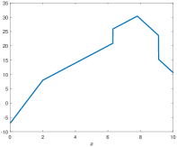
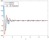
for every . Given a finite number of frequencies , , our interest lies in reconstructing an unknown piecewise affine signal from measurements of the form , , where denotes additive noise. This problem is severely ill-posed due to the gap between the infinite-dimensional nature of the unknown signal and the limited availability of measurements. For example, consider and the ground truth depicted in Figure 1(a). Its Fourier transform is sampled at eight equidistant points in , see Figure 1(b). Then there are , , such that the function
| (5.1) |
satisfies for all . Note that does not share any structural features of and even has a period smaller than due to the location of the first frequency measurement.
In order to preserve the piecewise affine linear structure of in the reconstruction and to alleviate the ill-posedness of this inversion, we thus propose to consider the -regularized problem
| (P) |
For abbreviation, define
as well as the linear and continuous observation operator
| (5.2) |
The following proposition addresses the existence of sparse minimizers to (P).
Proposition 12.
Proof.
Assumptions 1 (A1)-(A3) can be verified by direct calculations. In order to show (A4), let and with be arbitrary but fixed. Then there holds
for some depending on but not on . In the following denotes a generic constant which is independent of . We start by estimating
Denoting by the orthogonal complement of in and by , the respective orthogonal projections, we have
Now, estimating as in the proof of Proposition 1 and utilizing the continuous embedding , there holds
Moreover, using the injectivity of on , we get
Hence, combining both estimates, we conclude that the sublevel set is bounded. Since was chosen arbitrary, Assumption 1 (A4) follows. Thus, according to Proposition 10, Problem (P) admits at least one minimizer. Invoking Theorem 6 then yields the existence of minimizer of the form (3.1) with since and . The uniqueness of the optimal observation follows immediately from the strict convexity of . ∎
In the following, the optimal observation is denoted by . While Proposition 12 ensures the existence of at least one minimizer in the form (3.1), Corollary 1 implies that all solutions to (P) are sparse if the optimal misfit is nonzero.
Proof.
Let be an arbitrary minimizer to (P) and let denote the unique optimal observation. We readily verify that , and thus also and , (3.15), are analytic on due to
Moreover there holds since the functions , , are linearly independent and . The claimed statement now follows immediately from Corollary 1. ∎
In order to illustrate the advantages of solving Problem (P), we return to the setup described in Figure 1, i.e., we set
see Figure 1(a), and choose as well as , , as depicted in Figure 1(b). Subsequently, a measurement vector is generated by setting where is a noise vector with . The regularization parameters are chosen empirically as and . By direct computation, it is readily verified that is injective on in this case. Hence, Problem (P) admits a solution which can be computed using Algorithm 1.
5.1 Practical realization of Algorithm 1
Let us briefly discuss the practical realization of Algorithm 1 without discretizing the interval. For this purpose, we point out that , and admit a closed-form representation for every , . Hence, given the k-th iterate , the measurements , the corresponding derivative
as well as dual variables , see (4.3), can be computed without numerical approximation. Every iteration of Algorithm 1 then requires the solution of two subproblems. First, we have to determine global extrema of and in step 3. This is done by computing solutions of and using a Newton method starting at equally spaced points , . Then are chosen from the set of computed solutions by comparing the corresponding function values. Second, step 1 and 6, require the solution of the finite dimensional convex Problem . For this, we rely on a semismooth Newton method for the ”normal map” reformulation of its first order sufficient optimality conditions. In each iteration the method is warmstarted using the current iterate to construct a good starting point. Moreover we further enhance its practical performance by incorporating a heuristic globalization strategy based on damped Newton steps. The method is run for a maximum of iterations or until the constraint violation
satisfies for some . Note that, since (P) is convex, we also have
in virtue of Theorem 9. All of the following computations were carried out on Matlab 2019 on a notebook with GB RAM and an Intel®Core™ i7-10870H CPU@2.20 GHz.
5.2 Qualitative features of the reconstruction
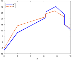
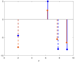
Starting from and , the method stops after iterations since . In Figure 2(a) we plot the computed function alongside the ground truth . We point out that is piecewise affine linear and its kinks and jumps closely approximate those of . At a first glance, it seems that both and share the same number of jumps/kinks. Upon a closer inspection, though, we observe that the kink at approximately is approximated by two kinks of equal sign in . We assume that this “clustering” behavior is a consequence of numerical rounding errors since the positions of both jumps/kinks only differ by a magnitude of order . Moreover, replacing both jumps/kinks by a single one of the combined magnitude at either of both candidate locations only introduces a relative error of in the objective functional value. In any case, the combined number of kinks and jumps in is considerably smaller than the theoretical upper bound of predicted by Proposition 12. Next, the reconstruction of the coefficients is investigated. For a better visualization, we plot a Dirac delta with weight , , at the position of the corresponding kink/jump (dashed lines for kinks, solid line for jumps) in Figure 2(b). The recovered function is treated analogously with the exception of merging the aforementioned clustering kinks into one of combined magnitude.
Observe that by solving (P) we successfully reconstruct the sign of every and provide decent estimates of its magnitude (after clustering). We also point out that, with the exception of the leftmost kink, the recovered coefficient is smaller than the reference. A possible explanation of this behavior can be found in Theorem 5 which states that the absolute values of the recovered coefficients are given by the solution to a minimization problem with an -type regularization term. For this type of problem, underestimation bias is a well-established phenomenon.
5.3 Optimality conditions and performance of Algorithm 1
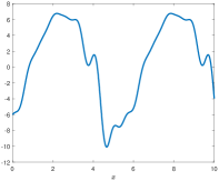
We take the opportunity and verify the structural properties of derived in Theorem 5. For this purpose, the dual variables and are plotted in Figures 3(a) and 3(b). Function values that correspond to the positions of jumps in are marked by orange dots in Figure 3(a). The same is done for function values corresponding to jumps in Figure 3(b).
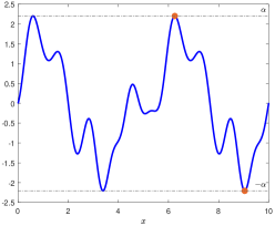
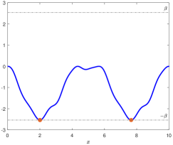
First, note that is nonzero. Hence, Theorem 4 implies that , . This is readily verified from the plots. Furthermore, the set of global extremas for each function consists of finitely many points. Consequently, the positions of jumps and kinks of align with minimizers/maximizers of and , respectively, as predicted by Theorem 5. Moreover the sign of the recovered coefficients for every jump/kink coincides with and , respectively, as expected.
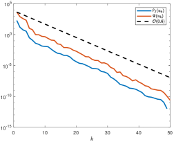
Finally, we plot the convergence of the constraint violation as well as of the residual
This approximation is justified by . The resulting graphs can be found in Figure 4(a). Clearly, these computations suggest a linear rate of convergence for both quantities which is vastly better than the and behavior predicted by Theorem 8 and 9, respectively. Alongside, in Figure 4(b), we plot the evolution of the active set size. Most remarkably, does not exceed throughout the iterations. This highlights the importance of the point removal step in Algorithm 1. Moreover, keeping small in combination with a warm-started semismooth Newton method leads to a fast resolution of the subproblems . In fact, the overall computation time of Algorithm 1 for the present example is merely s. In summary, these observations show the practical efficiency of methods in the spirit of Algorithm 1 for TGV-regularization. Of course, they also spark the demand of further research concerning e.g. an improved quantitative convergence analysis of Algorithm 1. However, since the focus of the present manuscript lies on the characterization of the extremal points and immediate consequences thereof, thorough investigations are postponed to a follow-up work.
Appendix A A counterexample
In this appendix we finally give the counterexample announced in Remark 4. More in detail, a set in as well as a convex and smooth function with are constructed. For this purpose, choose and with . Moreover set , and fix such that
Under this prerequisites, the function with and satisfies , see Remark 3. The following proposition provides an outline for the construction of a counterexample.
Proposition 13.
Assume that there is such that
| (A.1) |
Then is a minimizer of
| () |
for .
Proof.
In particular, if exists we have
due to . In order to construct such a function, define
Note that
as well as
Now, make the ansatz
| (A.3) |
The following proposition yields the desired counterexample.
Proposition 14.
There is such that satisfies (A.1).
Acknowledgments
We wish to thank Kristian Bredies for very interesting discussions and suggestions regarding the content of this work. The work of J.A.I. was partially supported by the State of Upper Austria.
References
- [1] L. Ambrosio, N. Fusco, and D. Pallara. Functions of bounded variation and free discontinuity problems. Oxford Mathematical Monographs. Oxford University Press, New York, 2000.
- [2] C. Boyer, A. Chambolle, Y. De Castro, V. Duval, F. De Gournay, and P. Weiss. On representer theorems and convex regularization. SIAM J. Optim., 29(2):1260–1281, 2019.
- [3] K. Bredies and M. Carioni. Sparsity of solutions for variational inverse problems with finite-dimensional data. Calc. Var. Partial Differential Equations, 59(1):14, 2020.
- [4] K. Bredies, M. Carioni, S. Fanzon, and D. Walter. Linear convergence of accelerated generalized conditional gradient methods. Preprint arXiv:2110.06756 [math.OC], 2021.
- [5] K. Bredies and M. Holler. Regularization of linear inverse problems with total generalized variation. J. Inverse Ill-Posed Probl., 22(6):871–913, 2014.
- [6] K. Bredies and M. Holler. Higher-order total variation approaches and generalisations. Inverse Probl., 36(12):123001, 128, 2020.
- [7] K. Bredies, K. Kunisch, and T. Pock. Total generalized variation. SIAM J. Imaging Sci., 3(3):492–526, 2010.
- [8] K. Bredies, K. Kunisch, and T. Valkonen. Properties of -: the one-dimensional case. J. Math. Anal. Appl., 398(1):438–454, 2013.
- [9] K. Bredies and T. Valkonen. Inverse problems with second-order total generalized variation constraints. In Proceedings of the 9th International Conference on Sampling Theory and Applications (SampTA), Singapore, 2011. arXiv:2005.09725.
- [10] E. Casas, C. Clason, and K. Kunisch. Parabolic control problems in measure spaces with sparse solutions. SIAM J. Control Optim., 51(1):28–63, 2013.
- [11] A. Chambolle and T. Pock. A first-order primal-dual algorithm for convex problems with applications to imaging. J. Math. Imaging Vision, 40(1):120–145, 2011.
- [12] J. C. De los Reyes and E. Loayza-Romero. Total generalized variation regularization in data assimilation for Burgers’ equation. Inverse Probl. Imaging, 13(4):755–786, 2019.
- [13] Y. Dong, T. Görner, and S. Kunis. An algorithm for total variation regularized photoacoustic imaging. Adv. Comput. Math., 41(2):423–438, 2015.
- [14] J. C. Dunn. Rates of convergence for conditional gradient algorithms near singular and nonsingular extremals. SIAM J. Control Optim., 17(2):187–211, 1979.
- [15] V. Duval, J.-F. Aujol, and Y. Gousseau. The TVL1 model: a geometric point of view. Multiscale Model. Simul., 8(1):154–189, 2009.
- [16] M. Fabian, P. Habala, P. Hájek, V. Montesinos Santalucía, J. Pelant, and V. Zizler. Functional analysis and infinite-dimensional geometry, volume 8 of CMS Books in Mathematics/Ouvrages de Mathématiques de la SMC. Springer-Verlag, New York, 2001.
- [17] M. Freiberger, C. Clason, and M. Scharfetter. Total variation regularization for nonlinear fluorescence tomography with an augmented lagrangian splitting approach. Appl. Opt., 49(19):3741–3747, 2010.
- [18] D. Kitahara, L. Condat, and A. Hirabayashi. One-dimensional edge-preserving spline smoothing for estimation of piecewise smooth functions. In ICASSP 2019 - 2019 IEEE International Conference on Acoustics, Speech and Signal Processing (ICASSP), pages 5611–5615, 2019.
- [19] H. Kuroda, M. Yamagishi, and I. Yamada. Exploiting sparsity in tight-dimensional spaces for piecewise continuous signal recovery. IEEE Trans. Signal Process., 66(24):6363–6376, 2018.
- [20] S. Lacoste-Julien. Convergence rate of Frank-Wolfe for non-convex objectives. Preprint arXiv:1607.00345 [math.OC], 2016.
- [21] Y. Nesterov. Introductory lectures on convex optimization, volume 87 of Applied Optimization. Kluwer Academic Publishers, Boston, MA, 2004.
- [22] G. Ongie and M. Jacob. Recovery of discontinuous signals using group sparse higher degree total variation. IEEE Signal Process. Lett., 22(9):1414–1418, 2015.
- [23] K. Papafitsoros and K. Bredies. A study of the one dimensional total generalised variation regularisation problem. Inverse Probl. Imaging, 9(2):511–550, 2015.
- [24] K. Papafitsoros and T. Valkonen. Asymptotic behaviour of total generalised variation. In Scale space and variational methods in computer vision, volume 9087 of Lecture Notes in Comput. Sci., pages 720–714. Springer, 2015.
- [25] C. Pöschl and O. Scherzer. Exact solutions of one-dimensional total generalized variation. Commun. Math. Sci., 13(1):171–202, 2015.
- [26] L. I. Rudin, S. Osher, and E. Fatemi. Nonlinear total variation based noise removal algorithms. Phys. D, 60(1-4):259–268, 1992.
- [27] I. W. Selesnick. Generalized total variation: Tying the knots. IEEE Signal Process. Lett., 22(11):2009–2013, 2015.
- [28] T. Valkonen. The jump set under geometric regularisation. Part 2: Higher-order approaches. J. Math. Anal. Appl., 453(2):1044–1085, 2017.