Abstract

Information-theoretic lower bounds are often encountered in several branches of computer science, including learning theory and cryptography. In the quantum setting, Holevo’s and Nayak’s bounds give an estimate of the amount of classical information that can be stored in a quantum state. Previous works have shown how to combine information-theoretic tools with a counting argument to lower bound the sample complexity of distribution-free quantum probably approximately correct (PAC) learning. In our work, we establish the notion of Probably Approximately Correct Source Coding and we show two novel applications in quantum learning theory and delegated quantum computation with a purely classical client. In particular, we provide a lower bound of the sample complexity of a quantum learner for arbitrary functions under the Zipf distribution, and we improve the security guarantees of a classically-driven delegation protocol for measurement-based quantum computation (MBQC).

Introduction

In recent years machine learning algorithms found impressive applications in several domains, ranging from automated driving, speech recognition, fraud detection and many others. Among the theoretical models proposed for the analysis of such algorithms, the probably approximately correct (PAC) learning is undoubtedly the most successful. Introduced in $1984$ by Leslie Valiant in the seminal work “A theory of the learnable” [1], this model is characterized by a twofold notion of error: given a target function $f$, the learner is required to output a hypothesis function $h$ which is close to $f$ up to a tolerance $\varepsilon$, with probability $1-\delta$.

The origins of quantum computation also find roots in the $1980$s, when Richard Feynman and others proposed harnessing quantum physics to create a novel model of computation [2, 3, 4]. Formalising this, we have now substantial theories built around this idea and how information can be transferred and processed in a quantum manner. This leads to quantum information theory and quantum computation respectively. In the modern day, Feynman’s vision is coming ever closer to realisation, in particular with the rapid development of small quantum computers. These devices with $\sim 80$ - $200$ qubits are dubbed noisy intermediate scale quantum (NISQ) [5] computers. On the quantum communication side, we also have proposals for a ‘quantum internet’, enabled by the secure transfer of quantum information across large distances [6]. This era poses two interesting challenges. On the one hand, due the low number of qubits and the experimental noise, these devices cannot perform many of the algorithms (or protocols on the communication side) thought to demonstrate exponential speedups over classical algorithms. Thus, the quest for practical applications gained momentum over the last years, especially in the field of quantum machine learning [7, 8, 9, 10, 11, 12]. On the other hand, NISQ devices are only accessibly via a ‘quantum cloud’ [13] and hence we need reliable protocols to delegate private computations.

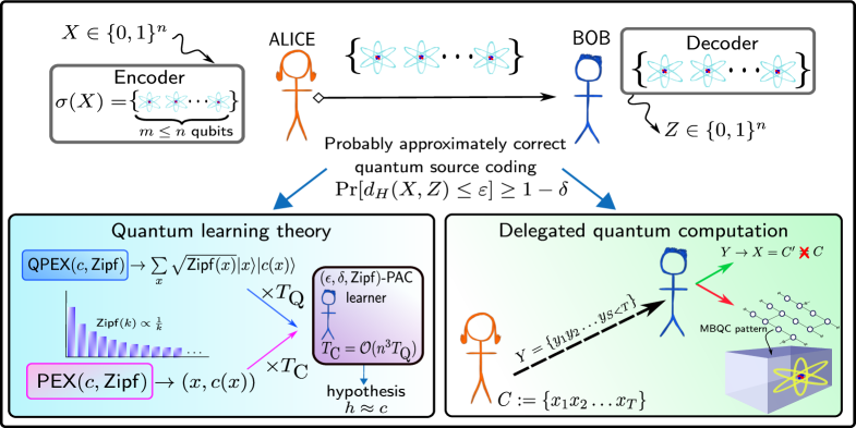
Figure 1: Probably approximately correct quantum source coding. An overview of PAC source coding and the two applications we study in this work. The results we derive place bounds on the receiver in a source coding protocol decoding the correct binary string, encoded in less qubits than information-theoretically required to perform a perfect decoding. The first application is in the quantum sample complexity of supervised learning under the $\mathsf{Zipf}$ distribution. Here, PAC source coding can be used to derive a sample complexity for quantum learners which may only be polylogarithmically better than using classical samples. The second is in proving bounds on the ability of an adversary in a delegated quantum computation protocol (in the measurement-based framework of quantum computing (MBQC)) to guess the client’s chosen computation.

Our contribution.

In this work, we demonstrate that the probably approximately correct approach can be employed in quantum information theory, providing applications in quantum learning theory and classically-driven delegated quantum computation.

First, we show that the quantum sample complexity and the classical sample complexity of the class of arbitrary functions under the Zipf distribution are equal, up to polylogarithmic factors. Moreover, we strengthen the security guarantee of the delegation protocol introduced in [14], bounding the probability that server reconstruct an approximated version of the target computation. Whereas we stated our bounds with respect to quantum states, the classical versions of our results can be recovered as special cases. Indeed, we believe that the application of our approach to classical computer science can be of independent interest.

Despite these practical applications, our major contribution is conceptual: our tools contribute to bridge the gap between information theory, machine learning and delegated computation, and they could ignite further advancement in the future.

Preliminaries

The term source coding refers to the process of encoding information produced by a given source in a way that it may be later decoded. The initial result of this topic, the source coding theorem, was derived in the seminal work of Shannon [15], which describes how many bits are required to encode independent and identically distributed random variables, without loss of information. One way to formalize this scenario is to consider a communication task, between two parties, Alice (A) and Bob (B). One generalisation of this theorem to the quantum world, is via Schumacher’s theorem [16, 17] which describes the number of qubits required to compress an $n$-fold tensor product of a quantum state, $\rho^{\otimes n}_{A}$, sent between Alice and Bob. In both cases, this number is directly related to the entropy of the random variable, or the quantum state. In the quantum scenario, the relevant quantity is the von Neumann entropy:

$$S(A):=S(\rho_{A}):=-\mathsf{tr}\left(\rho_{A}\log\rho_{A}\right)$$ (1)

This quantity generalises its classical counterpart, the Shannon entropy, which is the relevant object in the classical source coding theorem. From the entropy, one may define the mutual information, given in the quantum case by:

$$I(A;B):=S(A)+S(B)-S(AB)$$ (2)

We use the notation $S(AB)$ to mean the entropy of the state, $\rho_{AB}$, shared between Alice and Bob, and $\rho_{A}=\mathsf{tr}_{B}(\rho_{AB})$ is the reduced density matrix of this state with entropy, $S(A)$, and likewise for Bob.

However, all of the above applies to purely quantum sources, which is actually slightly too general for our purposes. Instead, we only require the source of Alice to quantumly encode classical information.

The setting is the following. Alice samples an $n$-bit random string, $X\xleftarrow{}\{0,1\}^{n}$, from some distribution, $p:\{0,1\}^{n}\rightarrow[0,1]$. She will then encode $X$ into a quantum state, $\sigma(X)\in\mathbb{C}^{d\times d}$ and send it to Bob. This defines an ensemble, $\Sigma:=\{\sigma(X),p(X)\}$. Finally, Bob performs a positive operator value measurement (POVM), $\mathbf{E}:=\{E_{m}\}_{m}$ on $\sigma$, and attempt to extract the encoded information. In reality, Bob will observe a string, $Z\in\{0,1\}^{n}$, and we wish to now bound the probability that he was successful, i.e. that $X=Z$.

First, we explore the minimum number of qubits Alice need to send to Bob to be successful in extracting the correct message? The answer comes from the Holevo’s bound [18] which states that the ‘accessible information’ of the ensemble, $\Sigma$, defined as:

$$I_{\text{Acc}}(\Sigma)=\max_{\mathbf{E}}I(X;Z)$$ (3)

is bounded by the ‘Holevo quantity’ of the ensemble, $\chi(\Sigma)$:

$$I_{\text{Acc}}(\Sigma)\leq\chi(\Sigma)\leq\log d$$ (4)

From the Holevo’s bound, we know that at least $n$ qubits are required to send a classical message of length $n$. However, what if we do not have access to $n$ qubits, but instead only $m<n$. Now, we have no chance to output the correct string with certainty, but we can aim to bound the probability of decoding the correct string. In this setting, we have the following result known as ‘Nayak’s bound’ [19]:

Lemma 1 (Nayak’s bound).

If $X$ is a $n$-bit binary string, we send it using $m$ qubits, and decode it via some mechanism back to an $n$-bit string $Z$, then our probability of correct decoding is given by:

$$\Pr[X=Z]\leq\frac{2^{m}}{2^{n}}=2^{m-n}.$$ (5)

Which intuitively states that our chance of correct decoding the string decreases exponentially with the difference between $m$ and $n$.

Next, we introduce three lemmata which shall be useful in our results. Firstly, as stated above, combinatorial tools play a central role in our treatment. As such, the following two bounds on binomial coefficients are relevant:

Lemma 2 (Binomial coefficient bounds).

The following two bounds on the binomial coefficients hold true:

$$\binom{n}{k}\leq 2^{nH\left(\frac{k}{n}\right)},\qquad\sum\limits_{i=0}^{m}\binom{n}{i}\leq 2^{nH\left(\frac{m}{n}\right)}~{}\forall m\leq\frac{n}{2},$$ (6)

where, for $0\leq p\leq 1$, $H(p)$ is the entropy of a binary random variable that takes value $1$ with probability $p$ and value $0$ with probability $1-p$, that is $H(p):=-p\log(p)-(1-p)\log(1-p)$.

Next, our second relevant lemma is an adaption of Theorem $15$ from [20].

Lemma 3.

For $\alpha\geq 0$, $\varepsilon\in[0,1/2)$, $\delta\in[0,1]$, assume that $I_{\text{Acc}}(\Sigma)\leq\alpha$ and $d_{H}(X,Z)\leq\varepsilon n$ with probability at least $1-\delta$. Then,

$$(1-\delta)[1-H(\varepsilon)]n-{H(\delta)}\leq\alpha.$$

Proof (adapted from [20])..

Since $I_{\text{Acc}}(\Sigma)\leq\alpha$, by definition of accessible information we have that:

$$I(X:Z)\leq\alpha.$$

Now, let $V$ be the indicator random variable for the event that $d_{H}(X,Z)\leq\varepsilon n$. Then $\Pr[V=1]\geq 1-\delta$. Conditioning to $V=1$ and given $Z$, $X$ can range over a set of only $\sum_{i=0}^{\varepsilon n}\binom{n}{i}\leq 2^{nH(\varepsilon)}$ $n$-bit strings (using Eq. (6)), we find that:

$$H(X|Z,V=1)\leq nH(\varepsilon)$$

We then lower bound $I(X:Z)$ as follows:

$$I(X:Z) =H(X)-H(X|Z)$$

$$\geq H(X)-H(X|Z,V)-H(V)$$

$$=H(X)-\Pr[V=1]H(X|Z,V=1)-\Pr[V=0]H(X|Z,V=0)-H(V)$$

$$\geq n-(1-\delta)H(\varepsilon)n-\delta n-H(\delta)$$

$$=(1-\delta)(1-H(\varepsilon))n-H(\delta).$$

Combining the two bounds we get the desired result:

$$(1-\delta)(1-H(\varepsilon))n-H(\delta)\leq\alpha.$$

∎

Finally, we recall the last lemma, from [21]:

Lemma 4 (Lemma 5 in [21]).

Let $m\geq 1$ be an integer and let $X,Y$ be correlated random variables. Let $\mu_{x}$ be the distribution of $Y|(X=x)$. Let $X^{\prime},Y^{\prime}$ represent joint random variables such that $X^{\prime}$ is distributed identically to $X$ and the distribution of $Y^{\prime}|(X^{\prime}=x)$ is $\mu^{m}_{x}$ ($m$ independent copies of $\mu_{x}$). Then,

$$I(X^{\prime}:Y^{\prime})\leq mI(X:Y).$$

Results

Now that we have discussed the required preliminaries, let us move to our results. To begin, let us recall how we discussed above that Nayak’s bound allows the string-decoding protocol to fail with some probability $0\leq\delta<1$. However, for our purposes, it is convenient to consider a further relaxation and the addition of a second error parameter, $0\leq\varepsilon<1$. We say that Alice and Bob succeed their task with probability $1-\delta$ up to an approximation error $\varepsilon$ if

$$\Pr[d_{H}(X,Z)\leq\varepsilon]\geq 1-\delta,$$

where $d_{H}$ is the Hamming distance between two strings of equal length, which is the number of positions at which the corresponding values are different.

In analogy with Probably Approximately Correct Learning as introduced above (and formalised in Sec. I), we refer to the above framework as Probably Approximately Correct Source Coding. In this context, we can prove the following generalization of the Nayak’s bound (Lemma 1).

Lemma 5 (PAC Nayak bound).

If $X$ is an $n$-bit binary string, we send it using $m$ qubits, and decode it via some mechanism back to an $n$-bit string $Z$ , then our probability of correct decoding up to an error $\beta n\geq 0$ in Hamming distance is given by

$$\Pr[d_{H}(X,Z)\leq\beta n]\leq\frac{2^{m}}{2^{n(1-\beta-H(\beta))}}.$$ (7)

Proof of Lemma 5.

The proof is straightforward, we begin by explicitly expanding the left hand side of Eq. (7):

$$\Pr[d_{H}(X,Z)\leq\beta n] =\Pr[\exists i_{1},\dots,i_{\lceil(1-\beta)n\rceil}:X_{i_{1}},\dots,X_{i_{\lceil(1-\beta)n\rceil}}=Z_{i_{1}},\dots,Z_{i_{\lceil(1-\beta)n\rceil}}]$$ (8)

$$\leq\binom{n}{\lfloor\beta n\rfloor}\Pr[X_{i_{1}},\dots,X_{i_{\lceil(1-\beta)n\rceil}}=Z_{i_{1}},\dots,Z_{i_{\lceil(1-\beta)n\rceil}}]$$ (9)

$$\leq 2^{H(\beta)n}\frac{2^{m}}{2^{n(1-\beta)}}=\frac{2^{m}}{2^{n(1-\beta-H(\beta))}},$$ (10)

We use the union bound for the second term in Eq. (9), and Eq. (6).

∎

Now, let us move from a success probability to a sample complexity result. In a PAC learning scenario, it is natural to assume that a classical message is transmitted through $m$ identical copies of a quantum state. This hypothesis stems from the definition of quantum sample reviewed in Eq. (14). Now, a natural question is to ask how many copies of such states are required in order to learn $X$ up to an error $\varepsilon$ in Hamming distance with probability $1-\delta$. We can derive the following lower bound from Holevo’s bound.

Lemma 6 (Learning a string with quantum data).

Let $\varepsilon\in[0,1/2)$. Assume $X$ is an $n$-bit binary string sampled with probability $p$, we send it using $m$ copies of a quantum state $\rho\in\mathbb{C}^{2^{\ell}\times 2^{\ell}}$ and decode it via some mechanism back to an $n$-bit string $Z$. Let $d_{H}(X,Z)\leq\varepsilon n$ with probability $1-\delta$. Then,

$$m\geq\frac{(1-\delta)(1-H(\varepsilon))n-H(\delta)}{\ell}$$

Proof.

By Lemma 4, we have that $I_{\text{Acc}}(\Sigma=\{\rho^{\otimes m},p\})\leq mI_{\text{Acc}}(\Sigma^{\prime}=\{\rho,p\})$. Moreover, we also have that $I_{\text{Acc}}(\Sigma^{\prime}=\{\rho,p\})\leq\ell$ by Eq. (4). By applying Lemma 3 and taking $\alpha:=m\ell$, we have that

$$(1-\delta)(1-H(\varepsilon))n-H(\delta) \leq m\ell.$$ (11)

$$\implies m \geq\frac{(1-\delta)(1-H(\varepsilon))n-H(\delta)}{\ell}$$ (12)

which completes the proof. ∎

Using the bounds above, we demonstrate two use cases in apparently distinct application areas. The first is an example in quantum learning theory, in which we prove a lower bound on the sample complexity of supervised learning algorithms relative to a specific distribution. The second is in the area of delegated quantum computation, where we use the bound to analyse and refine the security of the protocol of [14]. This protocol describes a method for a resource-limited ‘client’ to delegate a quantum computation to a powerful quantum ‘server’ in a manner to provide security guarantees to the data and information of the delegating client.

I Quantum learning theory

Before presenting our result, let us first briefly formalise our discussions of quantum learning theory, and how the above results can be useful there. As mentioned above, one of the most popular formalisms for a theory of learning is Probably Approximately Correct (PAC) learning. In PAC learning, one considers a concept class, usually Boolean functions, $\mathcal{C}\subseteq\mathcal{F}_{n}:=\{f|f:\{0,1\}^{n}\xrightarrow{}\{0,1\}\}$. For a given concept (given Boolean function to be learned), $c\in\mathcal{C}$, the goal of a PAC learner is to output a ‘hypothesis’, $h$, which is ‘probably approximately’ correct. In other words, the learner can output a hypothesis which agrees with the output of chosen function almost always. In order to be a ‘PAC learner for a concept class’, the learner must be able to do this for all $c\in\mathcal{C}$. In this process, learners are given access to an oracle, $O$, which outputs a sample from a distribution, $x\sim D$, along with the corresponding concept evaluation (the label) at that datapoint, $c(x)$. It is also important to distinguish between distribution-dependent learning, where $D$ is fixed, and distribution-free learning, where $D$ is arbitrary.

Now, we can formally define a PAC learner. Given a target concept class $\mathcal{C}$, a distribution $D$ and $\varepsilon,\delta\in[0,1]$, for any $c\in\mathcal{C}$ a $(\varepsilon,\delta,D)$-PAC learner outputs a hypothesis $h$ such that

$$\ell(c,h):=\Pr_{x\sim D}[c(x)\neq h(x)]\leq\varepsilon$$ (13)

with probability at least $1-\delta$.

In quantum PAC learning, we consider an alternative oracle $O^{\prime}$, as defined in [22], which outputs a quantum state that encodes both the concept class and the distribution, that is

$$\sum_{x\in\{0,1\}^{n}}{\sqrt{D(x)}}\ket{x}\ket{c(x)}.$$ (14)

A quantum oracle can easily simulate a classical one: it suffices to measure the first register of the state above in the computational basis. A key question is whether quantum learners may be able to learn concepts with a lower sample complexity than is possible classically. Early results in this direction were both positive and negative, with the distribution from which the examples are sampled being a crucial ingredient. For example, it was shown in [22] that exponential advantages for PAC learners were possible under the uniform distribution. On the other hand, in the distribution-free case, there is only a marginal improvement that quantum samples can hope to provide [20]. For our purposes, we analyse the sample complexity of quantum PAC learners, and use our tools to derive a lower bound on the learning problem, relative to another specific distribution (not simply the uniform one). The distribution in question is the Zipf distribution (which is a long-tailed distribution relevant in many practical scenarios, see [23, 24, 25] for example) over $\{0,1\}^{n}$, defined as follows:

$$\mathsf{Zipf}(k):=\frac{1}{kH_{N}},~{}H_{K}:=\sum\limits_{k=1}^{K}\frac{1}{k}\in[\log k,\log k+1]$$ (15)

In the following, we allow the target function to be completely arbitrary, i.e. we study the learnability of the concept class $\mathcal{F}_{n}$. Though this framework may look too simplistic, it captures prediction problems in which the domain doesn’t have any underlying structure. Examples of such structure could be a notion of distance on the domain. It has been thoroughly studied in [26], especially in relation to long-tailed distributions.

By applying Lemma 6, we can prove the following lower bound on the sample complexity of a quantum PAC learner for $\mathcal{F}_{n}$ relative to the Zipf distribution.

Theorem 1.

Let $N=2^{n}$ and $\beta\in[0,1/2]$. For every $\varepsilon\in[0,\frac{\beta}{n+1})$ and $\delta\in[0,1]$, every $(\varepsilon,\delta,\mathsf{Zipf})$-PAC quantum learner for $\mathcal{F}_{n}$ has sample complexity:

$$\Omega\left(\frac{(1-\delta)(1-H(\beta))N-H(\delta)}{n}\right).$$ (16)

Proof.

Firstly, let $h$ be the hypothesis produced by a quantum learner upon receiving $m$ quantum samples as in Eq. (14), such that $\ell(f,h)\leq\varepsilon$ with probability at least $1-\delta$.

In this proof, we represent the target function and the hypothesis in $N$-bit strings: $X=f(0)f(1)\dots f(N)$ and $Z=h(0)h(1)\dots h(N)$. Let $I$ be the subset of the indices where $X$ and $Z$ differ, i.e. $I:=\{i\in[N]:f(i)\neq h(i)\}$. The condition $\ell(f,h)\leq\varepsilon$ can be restated as:

$$\mathsf{Zipf}(I):=\sum_{i\in I}\mathsf{Zipf}(i)\leq\varepsilon<\frac{\beta}{n+1}.$$

Now we lower bound the quantity above.

$$\sum_{i\in I}\mathsf{Zipf}(i)\geq|I|\min_{i\in[N]}\mathsf{Zipf}(i)\geq\frac{|I|}{N(n+1)}.$$

Combining these two inequalities, we get that $|I|<\beta N<\nicefrac{{N}}{{2}}$. Furthermore, we can observe that that $d_{H}(X,Z)=|I|<\beta N$.

Finally, by Lemma 6, since quantum samples exist in $n$-qubit states, the sample complexity of quantum learner can be lower bounded as follows:

$$m\geq\frac{(1-\delta)(1-H(\beta))N-H(\delta)}{n},$$

which completes the proof. ∎

In particular, this result implies that we need at least ${O}(N/n)$ quantum samples to learn an arbitrary function under the Zipf distribution with approximation error $\varepsilon={O}(1/n)$.

Finally, for any distribution $D$ over $\{0,1\}^{n}$, we exhibit a $(\varepsilon,\delta,D)$-PAC classical learner for $\mathcal{F}_{n}$ with sample complexity $O\left(\frac{N}{\varepsilon}\log\frac{N}{\delta}\right)$. Informally, such learner memorizes the labels of the training examples, and assigns a random label to the remaining instances.

Theorem 2.

Let $N=2^{n}$ and let $D$ be a distribution over $[N]$. There exists a classical $(\varepsilon,\delta,D)$-PAC learner with sample complexity $O\left(\frac{N}{\varepsilon}\log\frac{N}{\delta}\right)$.

Proof.

We partition $X=[N]$ in two sets:

• $X_{1}:=\{i\in[N]:D(i)>\varepsilon/N\}$.

• $X_{2}:=\{i\in[N]:D(i)\leq\varepsilon/N\}$.

Observe that if $\forall x\in X_{1}:h(x)=f(x)$, then the generalization error is at most $\varepsilon$.

Fix $m:={\frac{N}{\varepsilon}\log\frac{N}{\delta}}$. Let $S=\{({i_{1}},f({i_{1}})),\ldots,({i_{m}},f({i_{m}}))$ be the examples.

The algorithm $\mathcal{A}$ works as follows:

1. For each point $i$ in the sample $S$, memorize its label $f(i)$.

2. Assign a random label to the points that aren’t in the sample $S$.

It suffices to prove that, with probability $1-\delta$, the sample covers all the points in $X_{1}$, i.e. $X_{1}\subseteq\{{i_{1}},\ldots,{i_{m}}\}$. Consider the probability of not obtaining a point $i\in X_{1}$ after $m$ queries, which is given by:

$$(1-D(i))^{m}\leq\left(1-\frac{\varepsilon}{N}\right)^{\frac{N}{\varepsilon}\log\frac{N}{\delta}}<e^{\log\frac{\delta}{N}}=\frac{\delta}{N},$$

where we employed the inequality $(1-\frac{1}{y})^{y}\leq\frac{1}{e}$ that is true for all $y\geq 1$. By the union bound, the probability that a point, $x$, in $X_{1}$ does not appear in the sample is given by

$$\Pr[\exists x\in X_{1}:x_{1}\not\in\{{i_{1}},\ldots,{i_{m}}\}]\leq\sum_{x\in X_{1}}\Pr[x\not\in\{{i_{1}},\ldots,{i_{m}}\}]\leq N\frac{\delta}{N}=\delta.$$

Thus, with probability at least $1-\delta$ every point in $X_{1}$ is contained the sample. ∎

The former result implies that we can learn an arbitrary function under an arbitrary distribution with approximation error $\varepsilon={O}(1/n)$ using at most ${O}(Nn^{2})$ classical samples.

Putting these together, we can observe that if we receive $T_{\text{Q}}$ quantum samples as in Eq. (14) according to the $\mathsf{Zipf}$ distribution, we can achieve the same learning error with $T_{\text{C}}=n^{3}T_{\text{Q}}$ classical samples, i.e. the sample complexity decreases by at most of a factor ${{O}}(n^{3})$.

II Classically-driven delegated quantum computation

In the previous sections, we demonstrated an application of our bounds in learning theory. Interestingly, the same mathematical tools can be applied in a completely different context, namely in the delegation of (quantum) computation. In this scenario, Alice takes the role of a ‘client’, who wishes to perform a quantum computation. However, she does not have the resources to to implement the computation herself, and therefore must delegate the problem to be solved to a ‘server’, Bob. However, for any number of reasons, the client may not trust the server, if even only to preserve their own privacy. This situation is extremely relevant in the current NISQ era, in which quantum computers do exist solely in the ‘quantum cloud’ [13] and will likely also be the norm for the near and far future, even perhaps when fully fault tolerant quantum computers are available. Delegated quantum computation has arisen to deal with this possibility and ensure computations are performed correctly and securely, with blind quantum computation being one of the primary techniques [27, 28, 29].

However, typically blind quantum computation requires Alice to have some minimal quantum resource, i.e. the ability to prepare single qubit states and send them to Bob. This presents its own issues however several efforts have been made to remove the quantum requirements from Alice [30, 31]. Doing so typically reduces the security of such delegation protocols from information-theoretic to simply computational in nature, based on primitives from post-quantum cryptography. Furthermore, based on assumptions in complexity theory, it is likely that information-theoretic security in this scenario is impossible without such quantum communication [32]. Nevertheless, it still may not be practical to demand quantum-enabled clients, and so in many cases classical communication to the server may be the best we can do.

In particular, we have in mind a protocol proposed by [14], which enables the delegation (by Alice) of a quantum computation to a remote server (Bob), using only classical resources (called classically driven blind quantum computing (CDBQC)). We remark that here the notion of blindness is weaker than in [27, 28, 29]. The CDBQC protocol is written in the language of measurement-based quantum computation (MBQC). Instead of using the quantum circuit model in which computation is driven by the operation of unitary evolutions on qubits, MBQC starts from a large entangled state (represented as a graph) and is driven by measurement of the qubits in the graph. In order to drive a blind computation, Alice needs to specify a set of measurement angles which describe the basis in which each qubit is measured.

Now, in the protocol of [14], she sends Bob $2n$ bits in order to convey this information. However, it is shown in [14] how $T:=3.388n$ bits are required to be send for Bob to have a complete specification of the MBQC computation. These extra bits are required to convey also the ‘flow information’ which is, roughly speaking, the manner in which the desired computation flows through the graph. The work of [14] essentially hides this flow information from the server, so Bob does not know which computation is actually desired by Alice. By applying Nayak’s bound (Lemma 1), the analysis of [14] shows that the probability that the server decodes the entire computation is at most $2^{-1.388n}\simeq 2^{-0.41T}$.

Using the tools derived above, we can further refine the claim of [14]. In particular, it is natural to ask whether the server can even guess a significant portion of the computation (rather than the entire computation as [14]). In many realistic scenarios, an adversary leaking any part of a computation can be a serious threat to the client’s privacy.

Now, by applying Lemma 3 and Lemma 5 we can derive the following result:

Theorem 3.

Let $\mathcal{C}$ be a family of computations, such that each $C\in\mathcal{C}$ can be encoded in a string of at least $T$ bits. Assume that a client delegates $C\in\mathcal{C}$ to a server using at most $0.591T$ bits of communication. Then the following bounds hold:

1. For every $\varepsilon\in[0,1]$, the server can guess $C$ up to an error $\varepsilon T$ in Hamming distance with probability at most $2^{(-0.41+\varepsilon+H(\varepsilon))T}$. This gives an exponentially small probability for every $\varepsilon<0.06$.

2. Assume that server outputs $C^{\prime}$ such that $d_{H}(C,C^{\prime})\leq\varepsilon T$ with probability $1$. Then $\varepsilon>0.08$.

Proof.

The first claim follows from a direct application of the PAC Nayak bound (Lemma 5). The server receives an input a string $Y$ of less than $0.591T$ bits, and she wants to decode a $T$-bit string $X$, with an approximation error of at most $\varepsilon T$ in Hamming distance. Hence, let $Z$ be a $T$-bit string output by the server. The success probability of a correct decoding is then given by:

$$P[d_{H}(X,Z)\leq\varepsilon T]\leq\frac{2^{0.591T}}{2^{T[1-\varepsilon-H(\varepsilon)]}}\leq 2^{[-0.41+\varepsilon+H(\varepsilon)]T}.$$

The second claim in Theorem 3 follows from an application of Lemma 3, choosing $\delta=0$ and combining with Eq. (4). The accessible information can be upper bounded by $0.591T$, and thus we have:

$$(1-H(\varepsilon))T \leq 0.591T$$

$$\implies\varepsilon >0.08.$$

∎

Conclusion

In summary, we have contributed to the field of quantum coding theory by incorporating tools from quantum learning theory. We developed a generalisation of Nayak’s bound, a fundamental result in quantum source coding by incorporating notions of error in decoding quantumly-encoded messages sent between two parties trying to communicate. We then showed two applications of the bound in distinct areas of quantum information and computation. The first was achieved by revisiting quantum learning theory, and describing the number of quantum samples required to learn a concept class, under a specific probability distribution, namely the Zipf distribution. The second example was in the field of delegated quantum computation, an area which is becoming increasing relevant due to the development of the quantum internet. Here, we refined the security of a protocol based on flow ambiguity in the measurement based model of quantum computation. For future work, obvious directions are to revisit and analyse scenarios in which the original form of Nayak’s bound is used, or by using our bounds to extend the study of quantum learning theory, for example deriving sample complexities under alternative distributions in the PAC model.

Furthermore, one could hope that the bounds discussed in this paper have not only application in the areas we have presented, but also in a range of other areas. The most likely candidates are those areas which involve, or can be modelled as, some form of quantum communication between two parties.

References

- Valiant [1984] L. G. Valiant. A theory of the learnable. Communications of the ACM, 27(11):1134–1142, November 1984. ISSN 0001-0782. doi: 10.1145/1968.1972. URL https://doi.org/10.1145/1968.1972.
- Benioff [1980] Paul Benioff. The computer as a physical system: A microscopic quantum mechanical Hamiltonian model of computers as represented by Turing machines. Journal of Statistical Physics, 22(5):563–591, May 1980. ISSN 1572-9613. doi: 10.1007/BF01011339. URL https://link.springer.com/article/10.1007/BF01011339. Company: Springer Distributor: Springer Institution: Springer Label: Springer Number: 5 Publisher: Kluwer Academic Publishers-Plenum Publishers.
- Feynman [1982] Richard P. Feynman. Simulating physics with computers. International Journal of Theoretical Physics, 21(6):467–488, June 1982. ISSN 1572-9575. doi: 10.1007/BF02650179. URL https://doi.org/10.1007/BF02650179.
- Preskill [2021] John Preskill. Quantum computing 40 years later. arXiv:2106.10522 [quant-ph], June 2021. URL http://arxiv.org/abs/2106.10522. arXiv: 2106.10522.
- Preskill [2018] John Preskill. Quantum Computing in the NISQ era and beyond. Quantum, 2:79, August 2018. doi: 10.22331/q-2018-08-06-79. URL https://quantum-journal.org/papers/q-2018-08-06-79/. Publisher: Verein zur Förderung des Open Access Publizierens in den Quantenwissenschaften.
- Wehner et al. [2018] Stephanie Wehner, David Elkouss, and Ronald Hanson. Quantum internet: A vision for the road ahead. Science, 362(6412):eaam9288, 2018. doi: 10.1126/science.aam9288. URL https://www.science.org/doi/abs/10.1126/science.aam9288.
- Biamonte et al. [2017] Jacob Biamonte, Peter Wittek, Nicola Pancotti, Patrick Rebentrost, Nathan Wiebe, and Seth Lloyd. Quantum machine learning. Nature, 549(7671):195–202, September 2017. ISSN 1476-4687. doi: 10.1038/nature23474. URL https://www.nature.com/articles/nature23474.
- Ciliberto et al. [2018] Carlo Ciliberto, Mark Herbster, Alessandro Davide Ialongo, Massimiliano Pontil, Andrea Rocchetto, Simone Severini, and Leonard Wossnig. Quantum machine learning: a classical perspective. Proceedings of the Royal Society A: Mathematical, Physical and Engineering Sciences, 474(2209):20170551, January 2018. doi: 10.1098/rspa.2017.0551. URL https://royalsocietypublishing.org/doi/10.1098/rspa.2017.0551.
- Adcock et al. [2015] Jeremy Adcock, Euan Allen, Matthew Day, Stefan Frick, Janna Hinchliff, Mack Johnson, Sam Morley-Short, Sam Pallister, Alasdair Price, and Stasja Stanisic. Advances in quantum machine learning. arXiv:1512.02900 [quant-ph], December 2015. URL http://arxiv.org/abs/1512.02900.
- Benedetti et al. [2019] Marcello Benedetti, Erika Lloyd, Stefan Sack, and Mattia Fiorentini. Parameterized quantum circuits as machine learning models. Quantum Science and Technology, 4(4):043001, November 2019. ISSN 2058-9565. doi: 10.1088/2058-9565/ab4eb5. URL https://doi.org/10.1088/2058-9565/ab4eb5.
- Bharti et al. [2021] Kishor Bharti, Alba Cervera-Lierta, Thi Ha Kyaw, Tobias Haug, Sumner Alperin-Lea, Abhinav Anand, Matthias Degroote, Hermanni Heimonen, Jakob S. Kottmann, Tim Menke, Wai-Keong Mok, Sukin Sim, Leong-Chuan Kwek, and Alán Aspuru-Guzik. Noisy intermediate-scale quantum (NISQ) algorithms. arXiv:2101.08448 [cond-mat, physics:quant-ph], January 2021. URL http://arxiv.org/abs/2101.08448.
- Arunachalam and de Wolf [2017] Srinivasan Arunachalam and Ronald de Wolf. Guest Column: A Survey of Quantum Learning Theory. ACM SIGACT News, 48(2):41–67, June 2017. ISSN 0163-5700. doi: 10.1145/3106700.3106710. URL https://doi.org/10.1145/3106700.3106710.
- LaRose [2019] Ryan LaRose. Overview and Comparison of Gate Level Quantum Software Platforms. Quantum, 3:130, March 2019. doi: 10.22331/q-2019-03-25-130. URL https://quantum-journal.org/papers/q-2019-03-25-130/.
- Mantri et al. [2017] Atul Mantri, Tommaso F. Demarie, Nicolas C. Menicucci, and Joseph F. Fitzsimons. Flow Ambiguity: A Path Towards Classically Driven Blind Quantum Computation. Phys. Rev. X, 7(3):031004, July 2017. doi: 10.1103/PhysRevX.7.031004. URL https://link.aps.org/doi/10.1103/PhysRevX.7.031004.
- Shannon [1948] C. E. Shannon. A Mathematical Theory of Communication. Bell System Technical Journal, 27(3):379–423, 1948. ISSN 1538-7305. doi: 10.1002/j.1538-7305.1948.tb01338.x. URL https://onlinelibrary.wiley.com/doi/abs/10.1002/j.1538-7305.1948.tb01338.x.
- Schumacher [1995] Benjamin Schumacher. Quantum coding. Phys. Rev. A, 51(4):2738–2747, April 1995. doi: 10.1103/PhysRevA.51.2738. URL https://link.aps.org/doi/10.1103/PhysRevA.51.2738.
- Jozsa and Schumacher [1994] Richard Jozsa and Benjamin Schumacher. A New Proof of the Quantum Noiseless Coding Theorem. Journal of Modern Optics, 41(12):2343–2349, December 1994. ISSN 0950-0340. doi: 10.1080/09500349414552191. URL https://doi.org/10.1080/09500349414552191.
- Holevo [1973] Alexander Holevo. Bounds for the Quantity of Information Transmitted by a Quantum Communication Channel. Problems of Information Transmission, 9(3):177–183, 1973.
- Nayak [1999] A. Nayak. Optimal lower bounds for quantum automata and random access codes. In 40th Annual Symposium on Foundations of Computer Science (Cat. No.99CB37039), pages 369–376, October 1999. doi: 10.1109/SFFCS.1999.814608.
- Arunachalam and Wolf [2018] Srinivasan Arunachalam and Ronald de Wolf. Optimal Quantum Sample Complexity of Learning Algorithms. Journal of Machine Learning Research, 19(71):1–36, 2018. URL http://jmlr.org/papers/v19/18-195.html.
- Jain and Zhang [2009] Rahul Jain and Shengyu Zhang. New bounds on classical and quantum one-way communication complexity. Theoretical Computer Science, 410(26):2463–2477, June 2009. ISSN 0304-3975. doi: 10.1016/j.tcs.2008.10.014. URL https://www.sciencedirect.com/science/article/pii/S0304397508007627.
- Bshouty and Jackson [1995] Nader H. Bshouty and Jeffrey C. Jackson. Learning DNF over the uniform distribution using a quantum example oracle. In Proceedings of the eighth annual conference on Computational learning theory, COLT ’95, pages 118–127, New York, NY, USA, July 1995. Association for Computing Machinery. ISBN 978-0-89791-723-0. doi: 10.1145/225298.225312. URL https://doi.org/10.1145/225298.225312.
- Zhu et al. [2014] Xiangxin Zhu, Dragomir Anguelov, and Deva Ramanan. Capturing Long-Tail Distributions of Object Subcategories. In 2014 IEEE Conference on Computer Vision and Pattern Recognition, pages 915–922, June 2014. doi: 10.1109/CVPR.2014.122. ISSN: 1063-6919.
- Zhang et al. [2017] Chiyuan Zhang, Samy Bengio, Moritz Hardt, Benjamin Recht, and Oriol Vinyals. Understanding deep learning requires rethinking generalization. In 5th International Conference on Learning Representations, ICLR 2017, Toulon, France, April 24-26, 2017, Conference Track Proceedings. OpenReview.net, 2017. URL https://openreview.net/forum?id=Sy8gdB9xx.
- Wang et al. [2017] Yu-Xiong Wang, Deva Ramanan, and Martial Hebert. Learning to Model the Tail. In I. Guyon, U. V. Luxburg, S. Bengio, H. Wallach, R. Fergus, S. Vishwanathan, and R. Garnett, editors, Advances in Neural Information Processing Systems, volume 30. Curran Associates, Inc., 2017. URL https://proceedings.neurips.cc/paper/2017/file/147ebe637038ca50a1265abac8dea181-Paper.pdf.
- Feldman [2020] Vitaly Feldman. Does learning require memorization? a short tale about a long tail. In Proceedings of the 52nd Annual ACM SIGACT Symposium on Theory of Computing, STOC 2020, page 954–959, New York, NY, USA, 2020. Association for Computing Machinery. ISBN 9781450369794. doi: 10.1145/3357713.3384290. URL https://doi.org/10.1145/3357713.3384290.
- Childs [2005] Andrew M. Childs. Secure assisted quantum computation. Quantum Information and Computation, 5(6), September 2005. ISSN 1533-7146. doi: 10.26421/qic5.6. URL http://dx.doi.org/10.26421/QIC5.6.
- Broadbent et al. [2009] Anne Broadbent, Joseph Fitzsimons, and Elham Kashefi. Universal Blind Quantum Computation. In 2009 50th Annual IEEE Symposium on Foundations of Computer Science, pages 517–526, October 2009. doi: 10.1109/FOCS.2009.36.
- Fitzsimons and Kashefi [2017] Joseph F. Fitzsimons and Elham Kashefi. Unconditionally verifiable blind quantum computation. Phys. Rev. A, 96(1):012303, July 2017. doi: 10.1103/PhysRevA.96.012303. URL https://link.aps.org/doi/10.1103/PhysRevA.96.012303.
- Gheorghiu and Vidick [2019] Alexandru Gheorghiu and Thomas Vidick. Computationally-Secure and Composable Remote State Preparation. In 2019 IEEE 60th Annual Symposium on Foundations of Computer Science (FOCS), pages 1024–1033, November 2019. doi: 10.1109/FOCS.2019.00066.
- Cojocaru et al. [2019] Alexandru Cojocaru, Léo Colisson, Elham Kashefi, and Petros Wallden. QFactory: Classically-Instructed Remote Secret Qubits Preparation. In Steven D. Galbraith and Shiho Moriai, editors, Advances in Cryptology – ASIACRYPT 2019, Lecture Notes in Computer Science, pages 615–645, Cham, 2019. Springer International Publishing. ISBN 978-3-030-34578-5. doi: 10.1007/978-3-030-34578-5˙22.
- Aaronson et al. [2019] Scott Aaronson, Alexandru Cojocaru, Alexandru Gheorghiu, and Elham Kashefi. Complexity-theoretic limitations on blind delegated quantum computation. arXiv:1704.08482 [quant-ph], February 2019. URL http://arxiv.org/abs/1704.08482.