BScNets: Block Simplicial Complex Neural Networks

Abstract

Simplicial neural networks (SNN) have recently emerged as the newest direction in graph learning which expands the idea of convolutional architectures from node space to simplicial complexes on graphs. Instead of pre-dominantly assessing pairwise relations among nodes as in the current practice, simplicial complexes allow us to describe higher-order interactions and multi-node graph structures. By building upon connection between the convolution operation and the new block Hodge-Laplacian, we propose the first SNN for link prediction. Our new Block Simplicial Complex Neural Networks (BScNets) model generalizes the existing graph convolutional network (GCN) frameworks by systematically incorporating salient interactions among multiple higher-order graph structures of different dimensions. We discuss theoretical foundations behind BScNets and illustrate its utility for link prediction on eight real-world and synthetic datasets. Our experiments indicate that BScNets outperforms the state-of-the-art models by a significant margin while maintaining low computation costs. Finally, we show utility of BScNets as the new promising alternative for tracking spread of infectious diseases such as COVID-19 and measuring the effectiveness of the healthcare risk mitigation strategies.

Introduction

Graph Convolutional Networks (GCNs) is a powerful machinery for graph learning, allowing for efficient exploration of various pairwise interactions among graph nodes. However, most GCN-based approaches tend to be limited in their ability to efficiently exploit and propagate information across higher-order structures (Morris et al. 2019; Xiao and Deng 2020). In turn, many recent studies on cyber-physical, social, and financial networks suggest that relations among multi-node graph structures, as opposed to pairwise interaction among nodes, may be the key toward understanding hidden mechanisms behind structural organization of complex network systems. For example, disease transmission might be influenced not only by one-to-one interactions but also be largely impacted by various group relations and social reinforcement induced by each person’s social circle, e.g., COVID-19 anti-mask and anti-vaccine views. To enhance the obfuscation efforts in money laundering schemes, criminals involve complex interactions not only among multiple individuals but also among multiple criminal groups. Such higher-order graph interactions beyond the node space and multi-node structures may be naturally modelled using simplicial complexes.

Simplicial neural networks (SNN) is the newly emerging direction in graph learning which extends convolutional operation to data that live on simplicial complexes. SNNs have recently been successfully applied to graph classification and trajectory forecasting (Ebli, Defferrard, and Spreemann 2020; Bunch et al. 2020; Roddenberry, Glaze, and Segarra 2021; Bodnar et al. 2021). The key engine behind SNNs is the Hodge–de Rham theory that generalizes the standard graph Laplacian which describes node-to-node interactions via edges to Hodge-Laplacian which allows us to model diffusion from edges to edges via nodes, edges to edges via triangles, triangles to triangles via edges, etc (Lim 2020; Schaub et al. 2020). Furthermore, Hodge-Laplacian establishes a natural connection between higher-order properties of discrete representations, e.g., graphs, and continuous representations, e.g., manifolds. As such, Hodge-Laplacian-based analytics opens multiple new perspectives for geometric representations at the interface of shape analysis, graph theory, and geometric deep learning (GDL) (Wang and Solomon 2019; Hajij, Istvan, and Zamzmi 2020).

In this paper we make the first step toward bridging SNNs with link prediction on graphs. We propose a new Block Simplicial Complex Neural Networks (BScNets) model, by building upon the connection between convolution operation and block Hodge-style representation. In contrast to other SNNs which tend to focus only on edge-to-edge information flows, or Hodge 1-Laplacian, BScNets allows us to simultaneously incorporate salient interactions among multiple simplicial complexes on graphs. Specifically, our BScNets scheme is composed of two components: the Adaptive Hodge Laplacian Based Block (AHLB) which describes multi-level structures and adaptively learns hidden dependencies among geometric representations of higher-order structures, and the Hodge-Style Adaptive Block Convolution (H-ABC) Module which automatically infers relations among multi-dimensional simplices. Our results indicate that this novel integration of information flows across not one but multiple higher-order structures via the Block Hodge Laplacian analytics yields the highest performance in link prediction tasks.

Significance and novelty of our contributions can be summarized as follows:

• Our BScNets is the first SNN for link prediction on graphs, bridging the recently emerging concepts of convolutional architectures on simplicial complexes with topological signal processing on graphs.

• We propose a new (random-walk based) adaptive Hodge Laplacian based block operator which simultaneously integrates knowledge on interactions among multiple higher-order graph structures and discuss its theoretical properties.

• We extensively validate BScNets on real-world and synthetic datasets, from such diverse domains as criminal, collaboration and transportation networks. Our results indicate that BScNets outperforms the state-of-the-art models by a significant margin while maintaining low computation costs.

• We discuss utility of BScNets and SNN tools as the new promising alternative for tracking spread of infectious diseases such as COVID-19 and evaluating healthcare risk mitigation strategies.

Related Work

Link Prediction GCN-based methods are known to be the powerful machinery for link prediction tasks. Specifically, the Graph Autoencoder (GAE) (Kipf and Welling 2016) and its variational version, i.e., Variational Graph Autoencoder (VGAE), are first employed to link prediction on citation networks. SEAL (Zhang and Chen 2018) extracts local enclosing subgraphs around the target links and learns a function mapping the subgraph patterns to link existence. In addition, the Hyperbolic Graph Convolutional Neural Networks (HGCN) (Chami et al. 2019) leverages both the hyperbolic geometry and GCN framework to learn node representations. Another interesting recent strategy is to use pairwise topological features to find latent representations of geometrical structure of graph using GCN (Yan et al. 2021). Our method differs from these approaches in that it explicitly models the higher-dimensional graph substructures and higher-order interactions via building an adaptive and interpretable Hodge block representation. Moreover, we propose a novel Hodge-style adaptive block convolution module to aggregate topological features encoded in the simplicial complexes by investigating relationships between simplices of different orders. This higher-order simplicial representation is substantially more general than the structural representation of node sets.

Simplicial Neural Networks Modeling higher-order interactions on graphs is an emerging direction in graph representation learning. While the role of higher-order graph structures for graph learning has been documented for a number of years (Agarwal, Branson, and Belongie 2006; Johnson and Goldring 2012) and involve such diverse applications as graph signal processing in electric, transportation and neuroscience systems, including link prediction (Benson et al. 2018), integration of higher-order graph substructures into deep learning on graphs has emerged only in 2020. Indeed, several most recent studies propose to leverage simplicial information to perform neural networks on graphs. For instance, Ebli, Defferrard, and Spreemann (2020) develops a model called Simplicial Neural Networks, which integrates the simplicial Laplacian of a simplicial complex into neural network framework based on simplicial Laplacian. Message Passing Simplicial Networks (MPSNs) (Bodnar et al. 2021) is proposed by performing massage passing on simplicial complexes for graph classification. Similarly, SCoNe (Roddenberry, Glaze, and Segarra 2021) uses the GCN architecture depended on simplicial complexes to extrapolate trajectories on trajectory data. Besides, the convolutional message passing scheme on cell complex (Hajij, Istvan, and Zamzmi 2020) is shown to facilitate representational learning on graphs. Our approach further advances these recent results by explicitly exploiting local topological information encoded in simplicial complexes of multiple dimensions and extracting the key interaction relations among multiple higher-order graph structures, which leads to significant gains in link prediction accuracy.

Block Simplicial Complex Neural Networks

We consider a graph $\mathcal{G}=\left(\mathcal{V},\mathcal{E},\boldsymbol{X}\right)$, where $\mathcal{V}$ is the set of nodes ($|\mathcal{V}|=n$) and $\mathcal{E}\subseteq\mathcal{V}\times\mathcal{V}$ is the set of edges ($|\mathcal{E}|=m$). Furthermore, each node $v_{i}$ is associated with a $d$-dimensional vector of attributes $\boldsymbol{x}_{i}$ which is the $i$-th row of matrix $\boldsymbol{X}\in\mathbb{R}^{n\times d}$ (where $d$ is the input feature dimension). Connectivity of $\mathcal{G}$ can be encoded in a form of an adjacency matrix $\boldsymbol{A}\in\mathbb{R}^{n\times n}$ with entries $[\boldsymbol{A}]_{ij}=1$ if nodes $i$ and $j$ are connected and 0, otherwise. For undirected graph $\mathcal{G}$, $\boldsymbol{A}$ is symmetric (i.e., $\boldsymbol{A}=\boldsymbol{A}^{\top}$).

Background on Hodge Theory One of the focal points of graph theory and, in virtue of it, GDL, is graph Laplacian. Laplacian allows us to establish a natural link between discrete representations, e.g., graphs, and continuous representations, e.g., manifolds (Chung and Graham 1997). The (unnormalized) graph Laplacian is defined as $\boldsymbol{L}_{0}=\boldsymbol{D}-\boldsymbol{A}$, and $\boldsymbol{L}_{0}$ is a symmetric and positive-semidefinite matrix. The Laplacian $\boldsymbol{L}_{0}$ represents a discrete counterpart of the Laplacian operator in vector calculus. In particular, as divergence of the gradient of some twice-differentiable multivariate function in vector calculus, the Laplacian operator is the flux density of the gradient flow of this function. That is, Laplacian measures how much the value of the function at any given point differs from average values of the function evaluated at nearby points. In turn, in the discrete case similarly, graph Laplacian $\boldsymbol{L}_{0}$ measures diffusion from node to node through edges and, broadly speaking, assesses at what extent the graph $\mathcal{G}$ differs at one node from the graph $\mathcal{G}$ at surrounding nodes. While $\boldsymbol{L}_{0}$ contains some very important information on the topology of $\mathcal{G}$, the natural question arises what if we are interested in diffusion dynamics on graph substructures beyond the node level? For example, formation of money laundering activities within criminal networks by default involves very complex multi-node interactions and, hence, cannot be well captured by methods that focus on the dyadic graph relationships. To assess such higher-order network properties, we can study graphs in terms of topological objects such as simplicial complexes and exploit the discrete Hodge theory, particularly, Hodge-Laplacian-based analytics as generalization of Laplacian dynamics to polyadic substructures of $\mathcal{G}$.

Definition 1

A family $\Delta$ of finite subsets of a set $\mathcal{V}$ is an abstract simplicial complex if for every $\sigma\in\Delta$, $\tau\subseteq\sigma$ implies $\tau\in\Delta$. I.e., $\Delta$ is closed under the operation of taking subsets. If $|\sigma|=k+1$, then $\sigma$ is called a $k$-simplex. Every subset $\tau\subset\sigma$ such that $|\sigma|=k$ is called a face of $\sigma$. All simplices in $\Delta$ that have $\sigma$ as face are called co-faces. Dimension of $\Delta$ is the largest dimension of any of its faces, or $\infty$ if there is no upper bound on the dimension of the faces.

Hence, nodes of $\mathcal{G}$ are 0-simplices, edges are 1-simplices, and triangles are 2-simplices. For a $k$-simplex of $k>0$, we can also define its orientation by (arbitrary) selecting some order for its nodes, and two orderings are said to be equivalent if they differ by an even permutation. As a result, for a given $k$-simplex $\sigma$ with orientation $[i_{0},i_{2},\ldots,i_{k}]$, any face of $\sigma$ is assigned its own orientation (or “identifyer”) $[i_{0},i_{1},\ldots,i_{j-1},i_{j+1},\ldots,i_{k}]$ (i.e., we omit the $j$-th element). To study diffusion among higher-order substructures of $\mathcal{G}$, we now form a real-valued vector space $C^{k}$ which is endowed with basis from the oriented $k$-simplices and whose elements are called $k$-chains. Diffusion through higher-order graph substructures can be then defined via linear maps among spaces $C^{k}$ of $k$-chains on $\mathcal{G}$ (Lim 2020).

Definition 2

A linear map $\partial_{k}:C^{k}\rightarrow C^{k-1}$ is called a boundary operator. The adjoint of the boundary map induces the co-boundary operator $\partial_{k}^{T}:C^{k}\rightarrow C^{k+1}$. Matrix representations of $\partial_{k}$ and $\partial_{k}^{\top}$ are $\boldsymbol{B}_{k}$ and $\boldsymbol{B}_{k}^{\top}$, respectively.

An operator over oriented $k$-simplices $\boldsymbol{L}_{k}:C^{k}\rightarrow C^{k}$ is called the $k$-Hodge Laplacian, and its matrix representation is given by

$$\boldsymbol{L}_{k}=\boldsymbol{B}_{k}^{\top}\boldsymbol{B}_{k}+\boldsymbol{B}_{k+1}\boldsymbol{B}_{k+1}^{\top},$$ (1)

where $\boldsymbol{B}_{k}^{\top}\boldsymbol{B}_{k}$ and $\boldsymbol{B}_{k+1}\boldsymbol{B}_{k+1}^{\top}$ are often referred to $\boldsymbol{L}^{down}_{k}$ and $\boldsymbol{L}^{up}_{k}$, respectively.

As $\boldsymbol{B}_{0}=0$, the standard graph Laplacian $\boldsymbol{L}_{0}$ is a subcase of (1) which tracks diffusion process from nodes to nodes via edges. Indeed, $\boldsymbol{L}_{0}=\boldsymbol{B}_{1}\boldsymbol{B}_{1}^{\top}$, where $\boldsymbol{B}_{1}$ is an $n\times m$-incidence matrix of $\mathcal{G}$ (i.e., $\boldsymbol{B}_{1}[ij]=1$ if node $i$ and edge $j$ are incident and 0, otherwise). In turn, $\boldsymbol{L}^{down}_{1}=\boldsymbol{B}_{1}^{\top}\boldsymbol{B}_{1}$ is often referred to as edge Laplacian and assesses diffusion from edges to edges via nodes. Finally, Hodge 1-Laplacian $\boldsymbol{L}_{1}$ measures variation on functions defined on graph edges (i.e., 1-simplices) with respect to the incidence relations among edges and nodes (i.e., 0-simplices) and edges and triangles (i.e., 2-simplices). More generally, $\boldsymbol{L}_{k}$ measures variation on functions defined on $k$-simplices of $\mathcal{G}$ with respect to incidence relations among $k$-simplices with $(k-1)$- and $(k+1)$-simplices. Figure 1 shows an example of the simplicial complex on a graph (more details are in Appendix A.1).

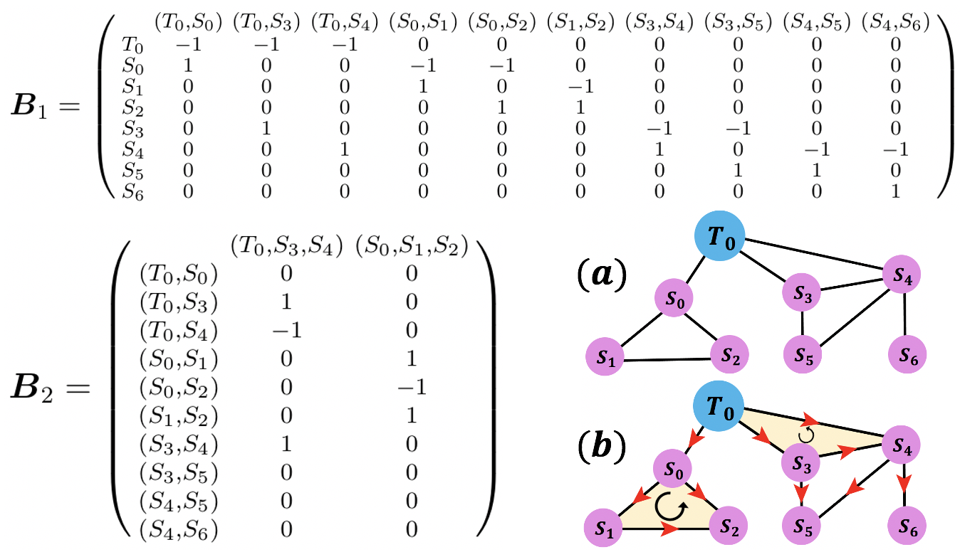
Figure 1: An example of generating simplicial complex from a classroom environment network, where $T_{0}$ is the teacher_0 and $S_{u}$ is the student_$u$ ($u\in\{0,\dots,6\}$). (a) Graph structure of the classroom environment network; (b) Simplicial complex of the classroom environment network; $\boldsymbol{B}_{1}$ and $\boldsymbol{B}_{2}$ are the corresponding node-to-edge and edge-to-face incidence matrices, respectively.

Random Walk Based Block Hodge-Laplacian Operator While the Hodge theory allows us to systematically describe diffusion across higher-order graph substructures, or $k$-simplices of any $k$, all current studies are restricted solely to Hodge 1-Laplacian $\boldsymbol{L}_{1}$ (Schaub et al. 2020; Roddenberry, Glaze, and Segarra 2021; Bodnar et al. 2021). In this paper we propose a new random walk based block Hodge-Laplacian operator which enables us to simultaneously integrate knowledge on interactions among higher-order substructures of various orders into graph learning.

Definition 3

The $K$-block Hodge-Laplacian $\boldsymbol{\mathfrak{L}}_{K}$ is a divergence operator on the direct sum of vector spaces $C^{k}$, $k\in\mathbb{Z}_{\geq 0}$. That is, $\boldsymbol{\mathfrak{L}}_{K}:\oplus_{k=0}^{K}C^{k}\rightarrow\oplus_{k=0}^{K}C^{k}$. Block Hodge-Laplacian $\boldsymbol{\mathfrak{L}}_{K}$ can be represented as a diagonal block matrix $\mathop{\mathrm{diag}}\{\boldsymbol{L}_{0},\boldsymbol{L}_{1},\ldots,\boldsymbol{L}_{K}\}$. Furthermore, by selecting a subset of indices $\{k_{1},\ldots,k_{j},\ldots,k_{J}\}\in\mathbb{Z}_{\geq 0}$, we can consider a reduced block Hodge-Laplacian ${}^{R}\boldsymbol{\mathfrak{L}}_{J}$, with a matrix representation $\mathop{\mathrm{diag}}\{\boldsymbol{L}_{k_{1}},\boldsymbol{L}_{k_{2}},\ldots,\boldsymbol{L}_{k_{J}}\}$, which allows us to describe interaction relations among a particular subset of higher-order graph substructures. Here positive integers $K$ and $k_{J}$ are bounded by the dimension of the abstract simplicial complex $\Delta$ on $\mathcal{G}$ and in practice, $K$ and $k_{J}$ are typically $\leq 2$.

The $K$-block Hodge-Laplacian $\boldsymbol{\mathfrak{L}}_{K}$ is related to the Dirac operator in differential geometry (i.e., Dirac operator is a square root of $\boldsymbol{\mathfrak{L}}_{K}$) (Lloyd, Garnerone, and Zanardi 2016). As such, $\boldsymbol{\mathfrak{L}}_{K}$ has multiple implications for analysis of synchronization dynamics and coupling of various topological signals on graphs, with applications in physics and quantum information processing (Calmon et al. 2021).

Lemma 1

For $K,J\in\mathbb{Z}_{\geq 0}$, operators $\boldsymbol{\mathfrak{L}}_{K}$ and ${}^{R}\boldsymbol{\mathfrak{L}}_{J}$ are symmetric and semipositive-definite, i.e. $\boldsymbol{\mathfrak{L}}_{K}\geq 0$ and ${}^{R}\boldsymbol{\mathfrak{L}}_{J}\geq 0$; $\boldsymbol{\mathfrak{L}}_{K}=(\boldsymbol{\mathfrak{L}}_{K})^{\top}$ and ${}^{R}\boldsymbol{\mathfrak{L}}_{J}=(^{R}\boldsymbol{\mathfrak{L}}_{J})^{\top}$.

Furthermore, we propose the random walk-based block Hodge-Laplacian, i.e., $r$-th power of block Hodge-Laplacian representation (where $r\in\mathbb{Z}_{>0}$). Our random walk-based block Hodge-Laplacian is inspired by the recent success in random walk based graph embeddings and simplicial complexes but is designed to conduct informative joint random walks on higher-order Hodge Laplacians instead of limited powering Hodge 1-Laplacian (Benson et al. 2018; Bodnar et al. 2021). Indeed, successfully travelling through higher-order topological features will provide us with additional feature information which is valuable for learning edge embeddings. The following Lemma 2 provides insight on the interplay among random walks on various $k$-simplices and their respective Hodge-Laplacian representation.

Lemma 2

For any $r\in\mathbb{Z}_{>0}$ and $K,J\in\mathbb{Z}_{\geq 0}$, the $r$-power of $(\boldsymbol{\mathfrak{L}}_{K})^{r}$ and $(^{R}\boldsymbol{\mathfrak{L}}_{J})^{r}$ are given by $\oplus_{k=0}^{K}((\boldsymbol{L}^{down}_{k})^{r}+(\boldsymbol{L}^{up}_{k})^{r})$ and $\oplus_{j=1}^{J}((\boldsymbol{L}^{down}_{k_{j}})^{r}+(\boldsymbol{L}^{up}_{k_{j}})^{r})$, respectively.

Adaptive Hodge Laplacian Based Block Analytics Our new approach to learning higher-order graph topology is motivated by the following question: Can we capture the interaction relations among $k$-simplices on the graph $\mathcal{G}$ whose orders are farther than $k-1$ and $k+1$ apart? While addressing this problem falls outside the Hodge-de Rham theory on the simplicial Hodge Laplacians, we provide an affirmative answer to this question through building an adaptive Hodge Laplacian Based Block Operator.

Without loss of generality, let us consider a 2-block (reduced) Hodge-Laplacian

$$\boldsymbol{\mathfrak{L}}_{2}=\left[\begin{array}[]{c|c}\boldsymbol{L}_{k_{1}}&O\\ \hline\cr O&\boldsymbol{L}_{k_{2}}\end{array}\right].$$ (4)

Our goal is to construct a new linear operator such that we describe interaction relations among $\boldsymbol{L}_{k_{1}}$ and $\boldsymbol{L}_{k_{2}}$. This problem can be addressed by defining and learning a similarity function $f(\boldsymbol{L}_{k_{1}},\boldsymbol{L}_{k_{2}})$. The natural choice for such similarity function is the inner product among elements in $C^{k_{1}}$ (i.e., $k_{1}$-chains) and elements in $C^{k_{2}}$ (i.e., $k_{2}$-chains). However, in general, $dim(C^{k_{1}})\neq dim(C^{k_{2}})$. Assume that $d_{1}=dim(C^{k_{1}})>d_{2}=dim(C^{k_{2}})$. Hence, instead we can consider a similarity function based on the inner product between elements in $C^{k_{2}}$ and elements in $\mathbb{P}_{d_{2}}C^{k_{1}}$, i.e., the projection of $C^{k_{1}}$ on the lower dimensional space. Here $\mathbb{P}_{d_{2}}$ is the corresponding orthogonal projector and, given symmetry of $\boldsymbol{L}_{k_{1}}$, can be formed by the eigenvectors of $\boldsymbol{L}_{k_{1}}$ corresponding to the top $d_{2}$ largest eigenvalues. Our new Adaptive Hodge Laplacian Based (AHLB) Block operator then takes the form

$$\boldsymbol{\mathbbm{L}}^{B}_{2}=\left[\begin{array}[]{c|c}\boldsymbol{L}_{k_{1}}&f(\mathbb{P}_{d_{2}}\boldsymbol{L}_{k_{1}},\boldsymbol{L}_{k_{2}})\\ \hline\cr f(\mathbb{P}_{d_{2}}\boldsymbol{L}_{k_{1}},\boldsymbol{L}_{k_{2}})^{\top}&\boldsymbol{L}_{k_{2}}\end{array}\right].$$ (7)

Note that in general, linear operator $\boldsymbol{\mathbbm{L}}^{B}_{2}\in\mathbb{R}^{(d_{1}+d_{2})\times(d_{1}+d_{2})}$ is no longer a Laplacian. For example, while $\boldsymbol{\mathbbm{L}}^{B}_{2}$ is symmetric (by construction), it may not satisfy the condition of positive semidefinitess (see Lemma 3 in Appendix A.2). However, as shown below, AHLB opens multiple opportunities to better describe higher-order interactions on graphs that are inaccessible not only with individual $k$-Hodge Laplacians but even with the $K$-block Hodge-Laplacian operator (see the ablation study for more details). In addition, followed by Lemma 2, we also consider a case when AHLB is constructed based on the $r$-th power of $\boldsymbol{\mathfrak{L}}_{2}$, and our studies indicate that on average the best results are achieved for $r=2$ (see Table 3 and Appendix A.3).

Armed with the AHLB operator (Eq. 7), we can utilize the non-local message operation $f(\cdot,\cdot)$ (Wang et al. 2018) to capture long-range relations and intrinsic higher-order connectivity among entities in the 2-block (reduced) Hodge-Laplacian $\boldsymbol{\mathfrak{L}}_{2}$, i.e., $f(\mathbb{P}_{d_{2}}\boldsymbol{L}_{k_{1}},\boldsymbol{L}_{k_{2}})$ placed in the off-diagonal. We now describe the choices of non-local message passing functions which can be used for $f(\cdot,\cdot)$ in the following. Specifically, given two higher-order Hodge Laplacians $\boldsymbol{L}_{k_{1}}$ and $\boldsymbol{L}_{k_{2}}$, we define two types of the non-local message passing functions to capture the relations between $[\mathbb{P}_{d_{2}}\boldsymbol{L}_{k_{1}}]_{i}\in\mathbb{R}^{d_{2}}$ and $[\boldsymbol{L}_{k_{2}}]_{j}\in\mathbb{R}^{d_{2}}$ (i.e., topological embedding of the $i$-th graph substructure in $\mathbb{P}_{d_{2}}\boldsymbol{L}_{k_{1}}$ and topological embedding of the $j$-th graph substructure in $\boldsymbol{L}_{k_{2}}$ respectively) as

(1) Inner-Product

$$f([\mathbb{P}_{d_{2}}\boldsymbol{L}_{k_{1}}]_{i},[\boldsymbol{L}_{k_{2}}]_{j})=<[\mathbb{P}_{d_{2}}\boldsymbol{L}_{k_{1}}]_{i},[\boldsymbol{L}_{k_{2}}]_{j}>.$$

Since all considered Laplacians in our case are over the real field $\mathbb{R}$, we can consider a dot-product. However, in a more general case of multivariable functions on graph simplices, $f(\cdot,\cdot)$ can be an inner-product.

(2) Embedded Inner-Product

$$f([\mathbb{P}_{d_{2}}\boldsymbol{L}_{k_{1}}]_{i},[\boldsymbol{L}_{k_{2}}]_{j})=<\boldsymbol{\Theta}_{\xi}[\mathbb{P}_{d_{2}}\boldsymbol{L}_{k_{1}}]_{i},\boldsymbol{\Theta}_{\psi}[\boldsymbol{L}_{k_{2}}]_{j}>,$$

where $\boldsymbol{\Theta}_{\xi}\in\mathbb{R}^{d_{c}\times d_{2}}$ and $\boldsymbol{\Theta}_{\psi}\in\mathbb{R}^{d_{c}\times d_{2}}$ are weight matrices to be learned, and $d_{c}$ is the embedding dimension. As such, we infer the relation value between two simplices.

Finally, the adaptive Hodge block can be formulated as

$$\tilde{\boldsymbol{\mathbbm{L}}}^{B}_{2}=\text{softmax}\left(\text{ReLU}\left(\boldsymbol{\mathbbm{L}}^{B}_{2}\right)\right),$$ (8)

where softmax function is applied to normalize the block operator $\boldsymbol{\mathbbm{L}}^{B}_{2}$, and the ReLU activation function (where $\text{ReLU}(\cdot)=\max{(0,\cdot)}$) eliminates both weak pairwise relation among higher-dimensional simplices and weak connections. As a result, the adaptive Hodge block $\tilde{\boldsymbol{\mathbbm{L}}}^{B}_{2}$ can dynamically learns interactions among simplices of different dimensions.

Hodge-Style Adaptive Block Convolution Module Armed with the AHLB operator, we now discuss how to construct the Hodge-style adaptive block convolution and use it to learn the distance between two nodes in the embedding space. Instead of using graph convolutional operator, i.e., $\boldsymbol{L}_{0}$, we adopt the AHLB operator $\tilde{\boldsymbol{\mathbbm{L}}}^{B}_{2}$ to demonstrate the effectiveness of the proposed novel higher-order Hodge convolution operator. The Hodge-style adaptive block convolution (H-ABC) module is given by

$${\boldsymbol{Z}^{(\ell+1)}}=\left(\tilde{\boldsymbol{\mathbbm{L}}}^{B}_{2}{\boldsymbol{Z}^{(\ell)}}{\boldsymbol{\Theta}^{(\ell)}_{1}}\right){\boldsymbol{\Theta}^{(\ell)}_{2}},$$ (9)

where $\boldsymbol{Z}^{(0)}=\boldsymbol{X}\in\mathbb{R}^{n\times d}$ is node features matrix, $\boldsymbol{\Theta}^{(\ell)}_{1}\in\mathbb{R}^{d\times(d_{1}+d_{2})}$ and $\boldsymbol{\Theta}^{(\ell)}_{2}\in\mathbb{R}^{(d_{1}+d_{2})\times d\textsubscript{out}}$ are two trainable weight matrices at layer $\ell$, and $d\textsubscript{out}$ denotes the dimension of node embedding at the $(\ell)$-th layer through the H-ABC operation. For the link prediction task, we use the Fermi-Dirac decoder (Nickel and Kiela 2017) to compute the distance between the two nodes. Formally,

$$\text{dist}^{\text{H-ABC}}_{uv}=({\boldsymbol{Z}^{(\ell+1)}_{u}-\boldsymbol{Z}^{(\ell+1)}_{v}})^{2},$$ (10)

where $\text{dist}\textsuperscript{H-ABC}_{uv}\in\mathbb{R}^{1\times d\textsubscript{out}}$ is the distance between nodes $u$ and $v$ in a local spatial domain.

Graph Convolution Layer Similar to the process of computing distances between learnable node embeddings with the Hodge-style adaptive block convolution, we also use graph convolution operation (Eq. 11) to evaluate the distance (Eq. 12) between the node embeddings of nodes $u$ and $v$ as

$${\boldsymbol{H}^{(\ell+1)}} =\tilde{\boldsymbol{L}}\boldsymbol{H}^{(\ell)}{\boldsymbol{\Theta}^{(\ell)}_{3}},$$ (11)

$$\text{dist}^{\text{GC}}_{uv} =({\boldsymbol{H}^{(\ell+1)}_{u}-\boldsymbol{H}^{(\ell+1)}_{v}})^{2},$$ (12)

where $\tilde{\boldsymbol{L}}={\boldsymbol{D}}_{v}^{-1/2}({\boldsymbol{A}+\boldsymbol{I}}){\boldsymbol{D}}_{v}^{-1/2}$ (where ${\boldsymbol{D}}_{v}$ is the degree matrix of $\boldsymbol{A}+\boldsymbol{I}$, i.e., $[\boldsymbol{D}_{v}]_{ii}=\sum_{j}[\boldsymbol{A}+\boldsymbol{I}]_{ij}$), $\boldsymbol{H}^{(0)}={\bf X}\in\mathbb{R}^{n\times d}$ is node features matrix, ${\boldsymbol{\Theta}^{(\ell)}_{3}}\in\mathbb{R}^{d\times d\textsubscript{out'}}$ is the trainable weight matrix, $d\textsubscript{out'}$ denotes the dimension of node embedding at the $(\ell)$-th layer through the graph convolution operation, $\text{dist}^{\text{GC}}_{uv}\in\mathbb{R}^{1\times d\textsubscript{out'}}$ is the distance between nodes $u$ and $v$ in global spatial domain.

Distance between Two Nodes We wrap the concatenation of Hodge-style adaptive convolution and graph convolution operation outputs (i.e., in Eqs. 10 and 12) into Multi-layer Perceptron (MLP) block

$$\text{dist}=\text{ReLU}(f_{\text{MLP}}([\pi_{\alpha}\times\text{dist}^{\text{GC}},\pi_{\beta}\times\text{dist}^{\text{H-ABC}}])),$$

where $[\cdot,\cdot]$ denotes the concatenation of the outputs from H-ABC module and graph convolution operation, $f_{\text{MLP}}$ is an MLP layer that maps the concatenated embedding to a $d_{o}$-dimensional space, and $\pi_{\alpha}$ and $\pi_{\beta}$ are the hyperparameters representing the weight of each distance (i.e., dist) in the $(\ell+1)$-th layer. Based on the propagation rule above, the edges connection probability can be computed as $prob(u,v)=\left[{\exp{((\text{dist}_{uv}-\delta)/\eta)}+1}\right]^{-1}$, where $\delta$ and $\eta$ are hyperparameters. Then, training via standard backpropagation is performed via binary cross-entropy loss function using negative sampling. Figure 2 illustrates our proposed BScNets framework, which consists of the Hodge-style adaptive block convolution module and graph convolution operation (see the Appendix A.4 for details).

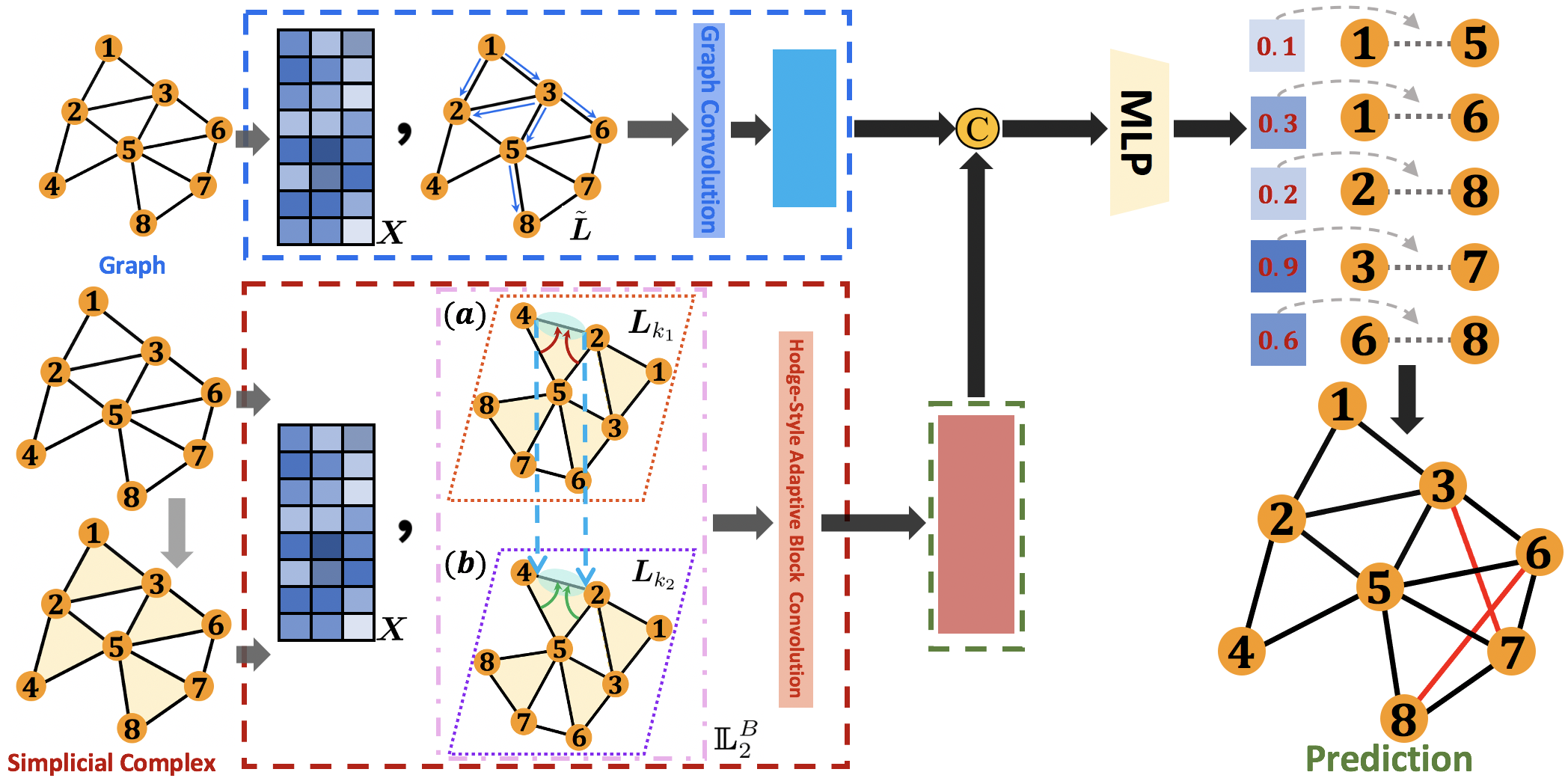
Figure 2: The architecture of BScNets. BScNets consists of graph convolution (upper row) and Hodge-style adaptive block convolution module (lower row). Each convolution layer/module contains the node feature matrix $\boldsymbol{X}$ and a Laplacian/operator (i.e., normalized Laplacian $\tilde{\boldsymbol{L}}$ and adaptive Hodge Laplacian based operator $\boldsymbol{\mathbbm{L}}^{B}_{2}$ for upper and lower parts respectively). Lower row presents the relation modeling between (a) Hodge Laplacian $\boldsymbol{L}_{k_{1}}$ describing diffusion from edge to edge through nodes and (b) Hodge Laplacian $\boldsymbol{L}_{k_{2}}$ describing diffusion from edge to edge through triangles. Symbol represents concatenation.

Experimental Study

Datasets We experiment on three types of networks (i) citation networks: Cora and PubMed (Sen et al. 2008); (ii) social networks: (1) flight network: Airport (Chami et al. 2019), (2) criminal networks: Meetings and Phone Calls (Cavallaro et al. 2020), and (3) contact networks: High School network and Staff Community (Salathé et al. 2010; Eletreby et al. 2020); (iii) disease propagation tree: Disease (Chami et al. 2019). The statistics and more details of the datasets are provided in Appendix B.1.1.

Baselines We compare against ten state-of-the-art (SOA) baselines, including (i) MLP, (ii) GCN (Kipf and Welling 2017), (iii) Simplified Graph Convolution (SGC) (Wu et al. 2019), (iv) Graph Attention Networks (GAT) (Veličković et al. 2018), (v) GraphSAG (SAGE), (vi) SEAL (Zhang and Chen 2018), (vii) Hyperbolic neural networks (HNN) (Ganea, Bécigneul, and Hofmann 2018), (viii) Hyperbolic Graph Convolutional Neural Networks (HGCN) (Chami et al. 2019), (ix) Persistence Enhanced Graph Neural Network (PEGN) (Zhao et al. 2020), and (x) Topological Loop-Counting Graph Neural Network (TLC-GNN) (Yan et al. 2021). Further details of baselines are contained in Appendix B.1.2.

Experiment Settings We implement our proposed BScNets with Pytorch framework on two NVIDIA RTX 3090 GPUs with 24 GiB RAM. Following (Chami et al. 2019), for all datasets, we randomly split edges into 85%/5%/10% for training, validation, and testing. Further, for all datasets, BScNets is trained by the Adam optimizer with the Cross Entropy Loss function. For all methods, we run 20 times with the same partition and report the average and standard deviation of ROC AUC values. More details about the experimental setup and hyperparameters are in Appendix B.2. Our datasets and codes are available on https://github.com/BScNets/BScNets.git.

Experiment Results Tables 1 and 2 show the comparison of our proposed BScNets with SOAs for link prediction tasks on six network datasets (i.e., Cora, PubMed, Meetings, Phone Calls, Airport, and Disease) and two contact network datasets (i.e., High School and Staff Community), respectively. The results indicate that our BScNets consistently achieves the best performance on all network datasets compared to all SOAs. Particularly, from Table 1, we find that: (i) Compared to the spectral-based ConvGNNs (i.e., GCN and SGC), BScNets yields more than 3.32% relative improvements to the existing best results for all six datasets; (ii) BScNets outperforms spatial-based ConvGNNs (i.e., GAT, SAGE, and SEAL) with a significant margin; (iii) Compared to the hyperbolic-based NNs (i.e., HNN and HGCN), BScNets improves upon HGCN (which performs best among the hyperbolic-based models) by a margin of 2.00%, 1.29%, 5.51%, 11.62%, 1.20% and 7.91% on datasets Cora, PubMed, Meetings, Phone Calls, Airport, and Disease, respectively; (iv) BScNets further improves PH-based ConvGNNs (i.e., PEGN and TLC-GNN) with a significant margin on all six datasets. Additionally, Table 2 shows performance of BScNets and baseline methods on High School network and Staff Community. BScNets obtains the superior results on all datasets, outperforming the representative spectral-, spatial-, PH-based models including GCN, SEAL, and TLC-GNN by a large margin. Based on the one-sided two-sample $t$-test, our BScNets also demonstrates statistically significant improvement in performance (marked by ^∗) compared to the existing best results in ROC AUC for all eight datasets (see Appendix B.5 for additional experimental results of BScNets).

Overall, the results show that BScNets can accurately capture the key structural information on the graph, both at the dyadic and polyadic levels of interactions, and achieves a highly promising performance in link prediction.

Table 1: ROC AUC and standard deviations for link prediction. Bold numbers denote the best results. ^∗ means statistically significant result.

Model	Cora	PubMed	Meetings	Phone Calls	Airport	Disease
MLP	83.15 $\pm$ 0.51	84.10 $\pm$ 0.97	63.20 $\pm$ 6.22	60.10 $\pm$ 6.72	89.51 $\pm$ 0.52	72.62 $\pm$ 0.61
HNN (Ganea, Bécigneul, and Hofmann 2018)	89.00 $\pm$ 0.10	94.87 $\pm$ 0.11	71.00 $\pm$ 3.28	60.90 $\pm$ 4.25	90.78 $\pm$ 0.22	75.10 $\pm$ 0.35
GCN (Kipf and Welling 2017)	90.42 $\pm$ 0.28	91.11 $\pm$ 0.55	72.08 $\pm$ 4.19	61.50 $\pm$ 5.80	89.27 $\pm$ 0.42	64.70 $\pm$ 0.56
GAT (Veličković et al. 2018)	93.89 $\pm$ 0.13	91.22 $\pm$ 0.12	74.00 $\pm$ 4.68	63.40 $\pm$ 5.20	90.55 $\pm$ 0.37	69.99 $\pm$ 0.32
SAGE (Hamilton, Ying, and Leskovec 2017)	86.24 $\pm$ 0.65	85.96 $\pm$ 1.16	72.30 $\pm$ 5.25	62.07 $\pm$ 5.49	90.47 $\pm$ 0.59	65.91 $\pm$ 0.33
SGC (Wu et al. 2019)	91.67 $\pm$ 0.20	94.10 $\pm$ 0.20	73.38 $\pm$ 3.49	63.80 $\pm$ 5.71	90.01 $\pm$ 0.32	65.21 $\pm$ 0.23
SEAL (Zhang and Chen 2018)	92.55 $\pm$ 0.50	92.42 $\pm$ 0.12	71.09 $\pm$ 7.50	62.96 $\pm$ 4.17	95.16 $\pm$ 0.39	85.23 $\pm$ 0.79
HGCN (Chami et al. 2019)	93.00 $\pm$ 0.45	96.29 $\pm$ 0.18	83.20 $\pm$ 4.15	70.20 $\pm$ 3.77	96.40 $\pm$ 0.19	90.80 $\pm$ 0.30
PEGN (Zhao et al. 2020)	93.13 $\pm$ 0.50	95.82 $\pm$ 0.20	74.17 $\pm$ 5.00	65.23 $\pm$ 4.15	95.46 $\pm$ 0.71	83.61 $\pm$ 1.26
TLC-GNN (Yan et al. 2021)	94.22 $\pm$ 0.78	97.03 $\pm$ 0.10	73.20 $\pm$ 5.32	66.17 $\pm$ 3.90	96.60 $\pm$ 0.69	86.19 $\pm$ 1.23
BScNets (ours)	∗94.90 $\pm$ 0.70	∗97.55 $\pm$ 0.12	∗88.05 $\pm$ 5.51	∗79.43 $\pm$ 6.04	∗97.57 $\pm$ 0.67	∗98.60 $\pm$ 0.58

Table 2: ROC AUC for link prediction on contact networks.

Model	High School	Staff Community
GCN (Kipf and Welling 2017)	63.55 $\pm$ 1.72	64.97 $\pm$ 6.88
SEAL (Zhang and Chen 2018)	68.13 $\pm$ 1.50	65.60 $\pm$ 3.46
HGCN (Chami et al. 2019)	67.30 $\pm$ 1.28	66.75 $\pm$ 1.38
TLC-GNN (Yan et al. 2021)	69.15 $\pm$ 1.49	67.35 $\pm$ 5.29
BScNets (ours)	∗71.68 $\pm$ 1.72	∗79.13 $\pm$ 2.95

Ablation Study To further investigate the importance of the different components in BScNets, we have conducted an ablation study of our proposed model on Cora and Disease and results are presented in Table 3 (^∗ means statistically significant result). We compare our BScNets with three ablated variants, i.e., (i) BScNets without random walk on block Hodge-Laplacian (W/o Random walks), (ii) BScNets without relation modeling (off-diagonal terms) (W/o Relation), and (iii) BScNets without the AHLB operator but with Hodge 1-Laplacian (With only $\boldsymbol{L}_{1}$; i.e., instead of using the block structure, we directly incorporate Hodge 1-Laplacian $\boldsymbol{L}_{1}$ into the Hodge-style convolution module by replacing $\tilde{\boldsymbol{\mathbbm{L}}}^{B}_{2}$ with $\boldsymbol{L}_{1}$ in Eq. 9). The results indicate that, when ablating the above components, the ROC AUC score of BScNets drops significantly. For both datasets, random walk mechanism on the block Hodge-style representation significantly improves the results as it utilizes higher-order relationships expressed in the graph data and learns embeddings beyond the node-space. In addition, we show that BScNets outperforms BScNets without relation modeling due to the fact that relation modeling integrates the learnt relationship between information in multi-dimensional simplices into the Hodge-style adaptive block convolutional encoder. Moreover, as expected, we find that replacing the AHLB operator by only Hodge 1-Laplacian results in a significant decrease in performance that indicates that block structure and off-diagonal higher-order relationships consistently boost the performance of link prediction.

Table 3: Ablation study of the network architecture (%).

Architecture	Cora	Disease
BScNets	∗94.90 $\pm$ 0.70	∗98.60 $\pm$ 0.58
W/o Random walk	93.79 $\pm$ 0.85	93.38 $\pm$ 5.85
W/o Relation	94.00 $\pm$ 0.60	95.90 $\pm$ 1.13
With $\boldsymbol{L}_{1}$	93.73 $\pm$ 0.44	93.43 $\pm$ 1.89

Computational Complexity Incidence matrices $\boldsymbol{B}_{1}$ and $\boldsymbol{B}_{2}$ can be calculated efficiently with the computational complexity $\mathcal{O}(n+m)$ and $\mathcal{O}(m+q)$ respectively, where $n$ is the number of 0-simplices (i.e., nodes), $m$ is the number of 1-simplices (i.e., edges), and $q$ is the number of 2-simplices (filled triangles). For large-scale graphs, we sample $\epsilon\times m$ edges (where $\epsilon\in(0,1]$) from edge set $\mathcal{E}$ and then pass these $\epsilon\times m$ edges to construct higher-order Hodge Laplacians. Thus this sparse sampling reduces the computation complexity of constructing $\boldsymbol{B}_{1}$ and $\boldsymbol{B}_{2}$ to $\mathcal{O}(n+\epsilon\times m)$ and $\mathcal{O}(\epsilon\times m+q^{\prime})$ respectively (where $q^{\prime}$ denotes the number of 2-simplices after sparse sampling). This sampling method is motivated by the DropEdge technique (Rong et al. 2019) which has been used to prevent over-fitting and over-smoothing in GCNs via randomly removing edges from the graph. Equipping BScNets with edge sampling results in substantial reductions in the size of the input data and, as such, computational complexity. Table in Appendix B.4 reports the average running time of incidence matrices generation for target network, training time per epoch of our BScNets model on all datasets, and running time comparison between BScNets and baselines.

Infectious Disease Transmission As recently noted by Iacopini et al. (2019); Schaub et al. (2020); Li et al. (2021), higher-order relationships such as multi-member group interactions, may be the key driving factors behind contagion dynamics, and simplicial complexes offer a natural way to describe such polyadic group relations. Here we are motivated by the two interlinked questions: Can we use link prediction with and without simplicial complexes to reconstruct unobserved social interactions and then to approximate the underlying contagion dynamics in the whole population? How accurate are the link prediction methods, with and without simplicial complexes, in reflecting the impact of disease mitigation strategies?

Indeed, in practice public healthcare professionals might have records on most registered residents (i.e., nodes) via, e.g., social security offices. However, there is only partial information on social interactions (i.e., edges) among these individuals. Our goals are to (i) predict social links among individuals where the interaction information is unknown, (ii) assess how mitigation strategies will impact the epidemic spread predicted from the reconstructed network, and (iii) evaluate how close the infection curves on the reconstructed data are to the infection curve on the whole true population. More details about the procedure of infectious disease transmission evaluation are provided in Appendix B.3.

We adopt the Susceptible-Exposed-Infected-Recovered (SEIR) (Kermack and McKendrick 1927) epidemic model. We set the infection curve delivered by SEIR on the whole population as the ground truth. We perturb certain fraction of links (i.e., remove the real links and add fake links) from the whole population to address the real world scenario when we do not have access to information on all social interactions. We then apply two link prediction methods to the network with perturbation, with and without simplicial complexes, BScNets and TLC-GNN, respectively. We now reconstruct the whole population by using BScNets and TLC-GNN and consider the two infection curves yielded by SEIR on the BScNets-based and TLC-GNN-based reconstructed networks. In addition, we assess sensitivity of the BScNets and TLC-GNN curves to mitigation strategies where more central nodes (individuals) are targeted to receive a vaccine, to quarantine or are persuaded to wear masks (Chen et al. 2021; Curiel and Ramírez 2021). Under the targeted mitigation strategies, a fraction of the most central nodes cannot transmit the disease. The ‘base’ infection curve is obtained from the whole population where such central nodes are removed from the disease spread. In turn, BScNets and TLC-GNN operate on the partially observed data where some edges are perturbed (as discussed above) and, upon reconstructing the unknown social interactions, BScNets and TLC-GNN are asked to re-determine their own individuals to be targeted through the disease mitigation strategy. We perform these experiments on the High School network (Salathé et al. 2010; Eletreby et al. 2020). We select TLC-GNN as the competing link prediction approach as it is a runner-up (see Table 2). We set the edge perturbation rate to 20%. We consider betweenness and degree centralities. We simulate each scenario 50 times and average the results. (For more experiments see Appendix B.3).

Figure 3 shows the infection curves during the time period of 180 days fitted to (i) the original network, (ii) the BScNets reconstructed network, and (iii) the TLC-GNN reconstructed network, under targeted mitigation strategy based on the betweenness centrality. We observe that the infection curve of the BScNets-reconstructed network (curve_BScNets) is significantly closer to the ‘base’ infection curve (i.e., curve_base) than the curve based on TLC-GNN (curve_runner-up). Most importantly, we find that while the peaks of the curve_BScNets and the curve_base are very close, i.e. 59.1% and 59.8%, respectively, the TLC-GNN curve (which does not account for multi-node group interactions) tends to substantially underestimate the number of infected individuals. For instance, at day $t=30$, $t=60$, $t=90$, $t=120$, and at day $t=180$, TLC-GNN suggests that only 0.5%, 2.2%, 10.1%, 29.5%, and 54.2% of population are infected, while the ground truth ‘base’ curve projects that 0.6%, 2.9%, 12.2%, 32.2%, and 59.8% are infected. That is, the difference between TLC-GNN and the ‘base’ curve, even for such small network, reaches 5% of the population, which eventually translates into significant societal implications such as shortages of health care facilities and overall system unpreparedness to pandemics like COVID-19. This phenomenon also confirms the most recent premise of epidemiological studies that higher-order interactions among multi-node groups (i.e., simplicial complexes) are the hidden driving factors behind the disease transmission mechanism. In turn, BScNets and other SNNs may be the most promising direction not only to capture such higher-order group interactions but also to reveal hidden polyadic relations in social networks.

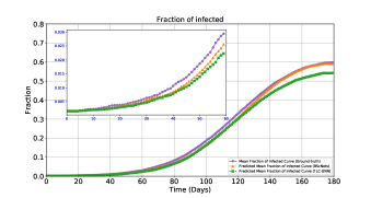
Figure 3: SEIR infection curves based on the original High School (HS) network (purple), BScNets-reconstructed HS network(orange), and TLC-GNN-reconstructed HS network (green), under betweenness-based mitigation strategy.

Conclusion

We have proposed the first SNN for link prediction. We have shown that relations among multiple multi-node structures play a significant role in graph learning. In the future, we will extend the ideas of simplicial DL to dynamic networks.

A. Methodology

A.1. Notations and Simplicial Complex Visualization

We summarize the main notations and their definitions in Table 4.

Table 4: The main symbols and definitions in this paper.

Notation	Definition
$\boldsymbol{A}$	adjacency matrix
$\boldsymbol{X}$	node feature matrix
$\boldsymbol{L}_{0}$	unnormalized graph Laplacian
$\boldsymbol{L}^{up}_{1}$	1-up-Laplacian
$\boldsymbol{L}^{down}_{1}$	edge Laplacian/1-down-Laplacian
$C^{k}$	vector space with the oriented $k$-simplices
$\partial_{k}$	boundary operator
$\boldsymbol{B}_{k}$	incidence matrix/matrix representation of $\partial_{k}$
$\boldsymbol{L}_{k}$	$k$-Hodge Laplacian
$\boldsymbol{\mathfrak{L}}_{K}$	$K$-block Hodge-Laplacian
${}^{R}\boldsymbol{\mathfrak{L}}_{J}$	reduced block Hodge-Laplacian
$\boldsymbol{\mathfrak{L}}_{2}$	2-block (reduced) Hodge-Laplacian
$\mathbb{P}_{d_{2}}$	orthogonal projector
$\boldsymbol{\mathbbm{L}}^{B}_{2}$	adaptive hodge Laplacian based block (AHLB)

We visualize an example of synthetic classroom environment network and its corresponding simplicial complex in Figure 4. The node $T_{0}$ (blue node) represents the teacher_0 and node $S_{u}$ (pink node) represents a student_$u$. The shaded areas represent the 2-simplices (triangles), i.e., $\{S_{0},S_{1},S_{2}\}$ and $\{T_{0},S_{3},S_{4}\}$. Besides, we show the orientation of each simplex graphically using arrows.

Figure 4: An example of generating simplicial complex from a classroom environment network, where $T_{0}$ is the teacher_0 and $S_{u}$ is the student_$u$ ($u\in\{0,\dots,6\}$). (a) Graph structure of the classroom environment network; (b) Simplicial complex of the classroom environment network; $\boldsymbol{B}_{1}$ and $\boldsymbol{B}_{2}$ are the corresponding node-to-edge and edge-to-face incidence matrices, respectively.

A.2. Lemmas and Proofs

Lemma 3

For $K,J\in\mathbb{Z}_{\geq 0}$, operators $\boldsymbol{\mathfrak{L}}_{K}$ and ${}^{R}\boldsymbol{\mathfrak{L}}_{J}$ are symmetric and semipositive-definite, i.e. $\boldsymbol{\mathfrak{L}}_{K}\geq 0$ and ${}^{R}\boldsymbol{\mathfrak{L}}_{J}\geq 0$; $\boldsymbol{\mathfrak{L}}_{K}=(\boldsymbol{\mathfrak{L}}_{K})^{\top}$ and ${}^{R}\boldsymbol{\mathfrak{L}}_{J}=(^{R}\boldsymbol{\mathfrak{L}}_{J})^{\top}$.

Proof Since for any nonnegative integer $i$, $\boldsymbol{L}_{i}=\boldsymbol{L}_{i}^{\top}$, by construction $\boldsymbol{\mathfrak{L}}_{K}=\boldsymbol{\mathfrak{L}}_{K}^{\top}$ and ${}^{R}\boldsymbol{\mathfrak{L}}_{J}=^{R}\boldsymbol{\mathfrak{L}}_{J}^{\top}$.

Positive semidefiniteness of $\boldsymbol{\mathfrak{L}}_{K}$ and ${}^{R}\boldsymbol{\mathfrak{L}}_{J}$ follows from the theorem on spectra of block upper/lower triangular partitioned matrices (see Simovici (2012)).

Lemma 4

For any $r\in\mathbb{Z}_{>0}$ and $K,J\in\mathbb{Z}_{\geq 0}$, the $r$-power of $(\boldsymbol{\mathfrak{L}}_{K})^{r}$ and $(^{R}\boldsymbol{\mathfrak{L}}_{J})^{r}$ are given by $\oplus_{k=0}^{K}((\boldsymbol{L}^{down}_{k})^{r}+(\boldsymbol{L}^{up}_{k})^{r})$ and $\oplus_{j=1}^{J}((\boldsymbol{L}^{down}_{k_{j}})^{r}+(\boldsymbol{L}^{up}_{k_{j}})^{r})$, respectively.

Proof In view of lemma 33 of Bodnar et al. (2021), for each nonnegative integers $r$ and $k$, $\boldsymbol{L}_{k}^{r}=(\boldsymbol{L}^{down}_{k}+\boldsymbol{L}^{up}_{k})^{r}=(\boldsymbol{L}^{down}_{k})^{r}+(\boldsymbol{L}^{up}_{k})^{r}$. The result of Lemma 2 then follows from the multiplication rule for block matrices (Eves 1980).

Consider the adaptive Hodge Laplacian Based (AHLB) Block operator

$$\boldsymbol{\mathbbm{L}}^{B}_{2}=\left[\begin{array}[]{c|c}\boldsymbol{L}_{k_{1}}&f(\mathbb{P}_{d_{2}}\boldsymbol{L}_{k_{1}},\boldsymbol{L}_{k_{2}})\\ \hline\cr f(\mathbb{P}_{d_{2}}\boldsymbol{L}_{k_{1}},\boldsymbol{L}_{k_{2}})^{\top}&\boldsymbol{L}_{k_{2}}\end{array}\right],$$ (15)

where the off-diagonal terms are defined via the embedded Inner-Product

$$f([\mathbb{P}_{d_{2}}\boldsymbol{L}_{k_{1}}]_{i},[\boldsymbol{L}_{k_{2}}]_{j})=<\boldsymbol{\Theta}_{\xi}[\mathbb{P}_{d_{2}}\boldsymbol{L}_{k_{1}}]_{i},\boldsymbol{\Theta}_{\psi}[\boldsymbol{L}_{k_{2}}]_{j}>.$$

Here $\boldsymbol{\Theta}_{\xi}\in\mathbb{R}^{d_{c}\times d_{2}}$ and $\boldsymbol{\Theta}_{\psi}\in\mathbb{R}^{d_{c}\times d_{2}}$ are weight matrices to be learned, and $d_{c}$ is the embedding dimension. Denote a $d_{c}\times d_{2}$-matrix $\boldsymbol{\Theta}_{\xi}[\mathbb{P}_{d_{2}}\boldsymbol{L}_{k_{1}}]$ as $\boldsymbol{W}$ and a $d_{c}\times d_{2}$-matrix $\boldsymbol{\Theta}_{\psi}\boldsymbol{L}_{k_{2}}$ as $\boldsymbol{U}$. Hence, since we consider Laplacians over the real field $\mathbb{R}$ and, as such, can use dot product, $\boldsymbol{\mathbbm{L}}^{B}_{2}$ can be re-written as

$$\boldsymbol{\mathbbm{L}}^{B}_{2}=\left[\begin{array}[]{c|c}\boldsymbol{L}_{k_{1}}&\boldsymbol{W}^{\top}\boldsymbol{U}\\ \hline\cr\boldsymbol{U}^{\top}\boldsymbol{W}&\boldsymbol{L}_{k_{2}}\end{array}\right].$$ (18)

Lemma 5

Given the adaptive Hodge Laplacian Based (AHLB) Block operator $\boldsymbol{\mathbbm{L}}^{B}_{2}$, the following conditions are equivalent:

1. $\boldsymbol{\mathbbm{L}}^{B}_{2}\geq 0$,

2. $\boldsymbol{U}^{\top}\boldsymbol{W}=\boldsymbol{L}_{k_{2}}\boldsymbol{L}_{k_{2}}^{\dagger}\boldsymbol{U}^{\top}\boldsymbol{W}$ and
   $\boldsymbol{L}_{k_{1}}-\boldsymbol{W}^{\top}\boldsymbol{U}\boldsymbol{L}_{k_{2}}^{\dagger}\boldsymbol{U}^{\top}\boldsymbol{W}\geq 0$,

3. $\boldsymbol{W}^{\top}\boldsymbol{U}-\boldsymbol{L}_{k_{1}}\boldsymbol{L}_{k_{1}}^{\dagger}\boldsymbol{W}^{\top}\boldsymbol{U}$ and
   $\boldsymbol{L}_{k_{2}}-\boldsymbol{U}^{\top}\boldsymbol{W}\boldsymbol{L}_{k_{1}}^{\dagger}\boldsymbol{W}^{\top}\boldsymbol{U}\geq 0$,

where $\boldsymbol{U}=\boldsymbol{\Theta}_{\psi}\boldsymbol{L}_{k_{2}}$, $\boldsymbol{W}=\boldsymbol{\Theta}_{\xi}[\mathbb{P}_{d_{2}}\boldsymbol{L}_{k_{1}}]$, and $\dagger$ denotes the Moore-Penrose inverse of a matrix. Here $\boldsymbol{L}_{k_{1}}-\boldsymbol{W}^{\top}\boldsymbol{U}\boldsymbol{L}_{k_{2}}^{\dagger}\boldsymbol{U}^{\top}\boldsymbol{W}$ and $\boldsymbol{L}_{k_{2}}-\boldsymbol{U}^{\top}\boldsymbol{W}\boldsymbol{L}_{k_{1}}^{\dagger}\boldsymbol{W}^{\top}\boldsymbol{U}$ are called Schur complements.

Proof Since $\boldsymbol{L}_{k_{2}}\geq 0$, $\boldsymbol{L}_{k_{1}}=\boldsymbol{L}_{k_{1}}^{\top}$ and $\boldsymbol{L}_{k_{2}}=\boldsymbol{L}_{k_{2}}^{\top}$, condition 3) is equivalent to condition i) of Theorem 1 by Albert (1969) (see p.435). Hence, by the Albert theorem, condition 3) holds iff $\boldsymbol{\mathbbm{L}}^{B}_{2}\geq 0$, that is, conditions 1) and 3) are equivalent.

In turn, since also $\boldsymbol{L}_{k_{1}}\geq 0$, from the Schur complement theorem, conditions 2) and 3) are equivalent (see p.263 of Bekker (1988)), which implies that conditions 1) and 2) are equivalent and concludes the proof.

A.3. Random walk-based $K$-block Hodge-Laplacian

In our experiments, followed by Lemma 2 (see main body part), we consider random walks on multiple simplices by generalizing Eq. 3 (see main body part) to arbitrary power $r$ (where $r\in\mathbb{Z}_{>0}$) gives

$$\boldsymbol{\mathbbm{L}}^{r}_{2}=\left[\begin{array}[]{c|c}\boldsymbol{L}^{r}_{k_{1}}&f(\mathbb{P}_{d_{2}}\boldsymbol{L}^{r}_{k_{1}},\boldsymbol{L}^{r}_{k_{2}})\\ \hline\cr f(\mathbb{P}_{d_{2}}\boldsymbol{L}^{r}_{k_{1}},\boldsymbol{L}^{r}_{k_{2}})^{\top}&\boldsymbol{L}^{r}_{k_{2}}\end{array}\right].$$

A.4. The overall framework of BScNets

The details of the architecture of our proposed BScNets are as follows. Figure 5 shows that in BScNets (i) the graph convolution is employed directly on graph-structured data to model node embeddings by aggregating the embeddings of neighbors and (ii) the Hodge-style adaptive block convolution module is constructed to jointly model edge embeddings via (1) message passing from edges to edges through nodes, (2) massage passing from edges to edges through triangles, and (3) relation modeling among Hodge representations from two simplicies. Lastly, we concatenate two corresponding embeddings and deploy a MLP to predict whether an edge exists between any pair of nodes.

Figure 5: The architecture of BScNets. BScNets consists of graph convolution (upper row) and Hodge-style adaptive block convolution module (lower row). Each convolution layer/module contains the node feature matrix $\boldsymbol{X}$ and a Laplacian/operator (i.e., normalized Laplacian $\tilde{\boldsymbol{L}}$ and adaptive Hodge Laplacian based operator $\boldsymbol{\mathbbm{L}}^{B}_{2}$ for upper and lower parts respectively). Lower row presents the relation modeling between (a) Hodge Laplacian $\boldsymbol{L}_{k_{1}}$ describing diffusion from edge to edge through nodes and (b) Hodge Laplacian $\boldsymbol{L}_{k_{2}}$ describing diffusion from edge to edge through triangles. Symbol represents concatenation.

B. Detailed Experimental Settings

B.1. Datasets and Baselines

B.1.1 Datasets

We experiment on three types of networks (i) citation networks: Cora and PubMed, (ii) social networks: Airport, Meetings, Phone Calls, High School network, Teacher Community, Staff Community, and (iii) disease propagation tree: Disease. Statistical overview of all eight datasets is in Table 5. We now provide the detailed descriptions of these three types of datasets we used as follows (i) Citation networks (i.e., Cora and Pubmed (Sen et al. 2008)) represent the citation relationship between two papers (where nodes represent papers and edges denote citation links) and node features are Bag-of-Words (BoW) representations of the papers. (ii) For social networks, (1) Airport (Chami et al. 2019) is a flight network dataset from openflights.org where nodes represent airports and edges represent the airline routes, (2) Meetings and Phone Calls are real criminal datastes built from juridical acts (Cavallaro et al. 2020): the Meetings network represents the physical meetings among members and the Phone Calls network represents phone calls between individuals (where nodes represent, e.g., members in the “Mistretta” family and the “Batanesi” clan and edges represent meetings or phone calls exchanged between pairs of individuals), (3) High School network and Staff Community: High School is the close proximity interaction (CPI) network observed at a U.S. high school during a typical day (Salathé et al. 2010) where nodes represent students, teachers, and staffs and edges represent interactions between two individuals; Staff Community is subnetwork contains nodes with staff label; following (Eletreby et al. 2020), we note that we sample a static graph out of the raw High School network by assigning an edge with the ratio of the total contact time between two nodes to the maximum total contact time observed in the dataset; it is noteworthy that social networks (i.e., Meetings, Phone Calls, High School network, and Staff Community) have no node attributes and thus we select four classic centralities as node features including degree, closeness centrality, betweenness centrality, and pagerank centrality. (iii) Disease propagation tree (Disease) (Chami et al. 2019) are simulated from the SIR model (Anderson and May 1992), where node attributes indicate the susceptibility to the disease and are generated through random sampling of Gaussian distributions (i.e., the mean and standard deviation are set for susceptible to disease and non-susceptible to disease, respectively). Table 5 summarizes the statistics of the datasets.

Table 5: Summary of datasets used in link prediction tasks.

Dataset	# Nodes	# Edges	# Features
Cora	2,708	5,429	1,433
PubMed	19,717	44,338	500
Meetings	101	256	4
Phone Calls	100	124	4
Airport	3,188	18,631	4
Disease	1,044	1,043	1,000
High School	773	6,342	4
Staff Community	55	441	4

B.1.2 Baselines

We compare against ten state-of-the-art (SOA) baselines, including (i) MLP: which is a feature-based approach to make link prediction without utilizing the graph structure information; (ii) two spectral-based convolutional GNNs (ConvGNNs): (1) GCN (Kipf and Welling 2017) and (2) Simplified Graph Convolution (SGC) (Wu et al. 2019) which simplifies the multi-layer graph convolutional networks by multiplying the adjacency matrix for $k$ times; (iii) three spatial-based ConvGNNs: (1) Graph Attention Networks (GAT) (Veličković et al. 2018) which adopts attention mechanism to aggregate the information from neighbors’ representation investigating the relative weights between two connected nodes, (2) GraphSAG (SAGE) which learns the node representations through sampling and aggregating features from its local neighborhood, and (3) SEAL (Zhang and Chen 2018) which predicts the relationship on graph-structure data based on graph convolution on local subgraph around each link; (iv) two hyperbolic-based NNs: (1) Hyperbolic neural networks (HNN) (Ganea, Bécigneul, and Hofmann 2018) which is the hyperbolic version of MLP and (2) Hyperbolic Graph Convolutional Neural Networks (HGCN) (Chami et al. 2019) which generalizes the graph convolution into hyperbolic space with aggregation in the tangent space; (v) two persistent homology (PH)-based ConvGNNs: (1) Persistence Enhanced Graph Neural Network (PEGN) (Zhao et al. 2020) which embeds topological information into the aggregation function and (2) Topological Loop-Counting Graph Neural Network (TLC-GNN) (Yan et al. 2021) which injects the pairwise topological information into the latent representation of a GCN.

B.2. Hyperparameter Settings and Training Details

BScNets consists of a one adaptive block Hodge convolution layer (nhid1) and two graph convolution layers (nhid2, nhid3), where nhid1 $\in\{1,8,16,32,64,128\}$, nhid2 $\in\{64,128,1024\}$, and nhid3 $\in\{4,16,32\}$. In addition, we perform an extensive grid search for learning rate among $\{0.001,0.005,0.008,0.01,0.05\}$, the dropout rate among $\{0.1,0.2,\dots,0.9\}$, power $r$ for random walk among $\{2,3,4,5\}$, and importance weights $\pi_{\alpha}$ among $\{0.01,0.1,1.0,10.0,100.0\}$ and $\pi_{\beta}$ among $\{1.0,10.0\}$ respectively. The model is trained for 5,000 epochs with early stopping applied when the metric (i.e., validation loss) starts to drop. We use ROC AUC as the metric for deriving the best hyperparameters and it is computed via cross-validation by the grid search. Furthermore, in Appendix B.7, we provide results of hyparameters sensitivity Analysis of $\delta$ and $\eta$.

B.3. Infectious Disease Transmission

We adopt the Susceptible-Exposed-Infected-Recovered (SEIR) epidemic model to investigate infectious disease transmission on High School network. In our simulation study, the parameters for SEIR model are as follows (i) transition rate ($S\rightarrow E$) $\beta=0.01$, (ii) transition rate ($E\rightarrow I$) $\alpha=0.1$, and (iii) recovery rate ($I\rightarrow R$) $\gamma=0.005$. For both betweenness- and degree-based mitigation strategies, the nodes are selected in the decreasing order of their corresponding betweenness centrality or degree centrality scores. In our experiments, we set 20% of nodes (i.e., individuals) under betweenness- or degree-based mitigation strategy, i.e., we remove 20% of nodes with highest betweenness centrality or degree centrality scores from the targeted network.

Besides, we also consider applying degree-based mitigation strategy on the original network, BScNets reconstructed network, and TLC-GNN reconstructed network respectively. Figure 6 shows the infection curves during the time period of 180 days fitted to (i) the original network, (ii) the BScNets reconstructed network, and (iii) the TLC-GNN reconstructed network, under targeted mitigation strategy based on the degree centrality. We find that the infection curves from the original network and BScNets reconstructed network are very close; however, the TLC-GNN curve (which does not account for multi-node group interactions) tends to substantially overestimate the number of infected individuals. For instance, at day $t=30$, $t=60$, $t=90$, $t=120$, and at day $t=180$, TLC-GNN suggests that only 0.6%, 2.7%, 11.1%, 30.5%, and 61.2% of population are infected, while the ground truth ‘base’ curve projects that 0.6%, 3.4%, 13.4%, 35.4%, and 61.4% are infected. This observation indicates that the decision-making (based on the estimation and forecasting from TLC-GNN) may result in time consuming and resource wasting for governments and public agencies.

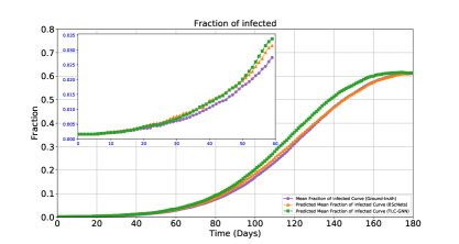
Figure 6: SEIR infection curves based on the original High School (HS) network (purple), BScNets-reconstructed HS network(orange), and TLC-GNN-reconstructed HS network (green), under betweenness-based mitigation strategy.

B.4. Computation Complexity

Table 11 shows the computational costs for incidence matrices generation and training time per epoch of our BScNets on all eight datasets. We have shown that our BScNets equipped with the sparse sampling technique is much more efficient in terms of running time. For instance, the number of edges in PubMed is more than 16 times larger than the number of edges in Cora; however, the incidence matrices generation of PubMed exceeds the incidence matrices generation of Cora with more than 165 less computation cost (running time). In summary, our BScNets model can be conducted on large-scale real-world datasets (static and dynamic) without the issues running of out-of-memory and prohibitive computational costs. Besides that, we then further report the running time (in seconds) of BScNets and 4 baselines on Cora and Disease. We can see that BScNets outperforms baselines and maintains comparable running time.

Table 6: Link prediction in ROC AUC on Citeseer.

Dataset	BScNets	DeepWalk	Node2Vec	Node2Vec-GCN	GCN	SEAL	HGCN	TLC-GNN
CiteSeer	96.32$\pm$0.95	79.28$\pm$0.80	79.60$\pm$0.75	85.05$\pm$0.83	84.67$\pm$1.80	80.79$\pm$0.79	94.03$\pm$0.59	95.11$\pm$0.97

Table 7: Link prediction in ROC AUC on PPI.

Dataset	BScNets	SkipGNN	DEAL	SAGE	SEAL	GCN	GAT
PPI	89.19$\pm$0.16	87.77$\pm$0.17	88.56$\pm$0.20	81.15$\pm$0.12	88.19$\pm$0.19	83.65$\pm$0.15	81.79$\pm$0.18

Table 8: Hits@20 and Hits@50 score on OGBs with the 5% and 10% training sets.

Dataset	Ratio	BScNets	GCN	SAGE	LRGA
OGBL-DDI	5%	25.52$\pm$0.03	23.30$\pm$0.05	13.93$\pm$0.05	22.02$\pm$0.09
OGBL-DDI	10%	31.53$\pm$0.08	25.13$\pm$0.06	26.41$\pm$0.08	28.69$\pm$0.12
OGBL-COLLAB	5%	27.09$\pm$0.08	24.87$\pm$0.07	18.26$\pm$0.09	21.39$\pm$0.15
OGBL-COLLAB	10%	31.00$\pm$0.08	27.08$\pm$0.05	21.71$\pm$0.03	27.12$\pm$0.10

Table 9: Training time (per epoch in seconds).

Dataset	BScNets	GCN	SEAL	HGCN	TLC-GNN
Cora	$7.04\times 10^{-2}$	$5.35\times 10^{-2}$	$5.76\times 10^{-1}$	$1.13\times 10^{-2}$	$1.01\times 10^{-1}$
Disease	$3.50\times 10^{-2}$	$1.42\times 10^{-2}$	$1.97\times 10^{-1}$	$1.31\times 10^{-1}$	$8.13\times 10^{-2}$

Table 10: Hyparameters sensitivity analysis of $\delta$ and $\eta$ on Disease dataset.

Dataset	($\delta=2,\eta=1$)	($\delta=0.1,\eta=1$)	($\delta=3,\eta=1$)	($\delta=2,\eta=2$)	($\delta=2,\eta=5$)
Disease	98.60$\pm$0.58	98.28$\pm$0.50	98.18$\pm$0.72	98.31$\pm$0.63	98.29$\pm$0.63

Table 11: Computational costs for generation of incidence matrices (i.e., $\boldsymbol{B}_{1}$ and $\boldsymbol{B}_{2}$) and a single training epoch of BScNets.

Dataset	Average Time Taken (sec)
	Incidence matrices	BScNets (epoch)
Cora	$7.00\times 10^{-3}$	$7.04\times 10^{-2}$
PubMed	$4.22\times 10^{-5}$	$8.75\times 10^{-2}$
Meetings	$7.55\times 10^{-4}$	$5.61\times 10^{-2}$
Phone Calls	$5.08\times 10^{-5}$	$4.06\times 10^{-3}$
Airport	$3.36\times 10^{-4}$	$2.47\times 10^{-2}$
Disease	$3.81\times 10^{-6}$	$3.50\times 10^{-2}$
High School	$1.21\times 10^{-3}$	$3.66\times 10^{-2}$
Staff Community	$5.25\times 10^{-3}$	$1.14\times 10^{-2}$

B.5. Additional Experiments

We now have also run experiments on large datasets and datasets with rich node attributes, i.e., CiteSeer, protein–protein interaction (PPI), OGBL-DDI, and OGBL-COLLAB. CiteSeer is proposed in (Sen et al. 2008). PPIs is proposed in (Zitnik and Leskovec 2017). OGBL-DDI and OGBL-COLLAB are proposed in (Hu et al. 2020). The statistics of these datasets are given in Table 12. For the experimental results on CiteSeer and PPI, we randomly split edges into 80%/10%/10% for training, validation, and testing, and report the mean average area under the ROC curve (ROC AUC) score (with 5 independent runs). For OGBL-DDI and OGBL-COLLAB, we randomly select $\rho$% of edges as the training set (where $\rho=\{5,10\}$), and we use 10% for both validation and test sets (with an equal # of true and false edges). The evaluation metric is called Hits@K (Hu et al. 2020) (where K$=\{20,50\}$). Tables 6 and 7 summarize the performance of BScNets and SOAs on CiteSeer and PPIs (we also select several representative baselines to compare including Node2Vec (Grover and Leskovec 2016), Node2Vec-GCN (Yadati et al. 2020), DEAL (Hao et al. 2020), and SkipGNN (Huang et al. 2020)). We can observe that BScNets consistently achieves large-margin outperformance over all baselines across both CiteSeer and PPI. The results on OGBL-DDI and OGBL-COLLAB are presented in Table 8. We observe that BScNets outperforms GCN, SAGE, and LRGA (Puny, Ben-Hamu, and Lipman 2020) on both OGBs.

Table 12: Summary of additional datasets.

Dataset	# Nodes	# Edges	# Features
CiteSeer	3,327	4,552	3,703
PPI	1,767	16,159	50
OGBL-DDI	4,267	1,334,889	0
OGBL-COLLAB	235,868	1,285,465	128

Besides transductive learning, following the data splitting setting of (Hao et al. 2020), we also conduct the experiment on Citeseer based on the inductive framework of (Hao et al. 2020) with BScNets for the message passing module. Table 13 shows that BScNets also outperforms all baselines for inductive learning.

Table 13: Inductive link prediction in ROC AUC on Citeseer.

Dataset	BScNets	DEAL	SAGE	G2G	MLP
Citeseer	95.85$\pm$0.17	93.70$\pm$0.21	89.21$\pm$0.26	92.13$\pm$0.26	87.70$\pm$0.66

B.6. Ablation Study on the GCN Layer

We further perform the ablation study to the effect of the graph convolution operator (i.e., BScNets w/o GCN layer) on Cora and Disease. As Table 14 shows, BScNets with GCN layer performs better than w/o GCN layer. The results show importance of capturing essential info at the node-level.

Table 14: Ablation study on the GCN layer.

Dataset	BScNets	BScNets w/o GCN Layer
Cora	94.90$\pm$0.70	90.59$\pm$0.75
Disease	98.60$\pm$0.58	98.13$\pm$0.65

B.7. Hyparameters Sensitivity Analysis of $\delta$ and $\eta$

Table 10 shows hyperparameters sensitivity for $\delta$ and $\eta$ on Disease. We find that BScNets with $(\delta=2,\eta=1)$ yields a relative gain from 0.29% to 0.43% in terms of ROC AUC over BScNets with other $(\delta,\eta)$ hyperparameter combinations.

References

- Agarwal, Branson, and Belongie (2006) Agarwal, S.; Branson, K.; and Belongie, S. 2006. Higher order learning with graphs. In ICLR, 17–24.
- Albert (1969) Albert, A. 1969. Conditions for positive and nonnegative definiteness in terms of pseudoinverses. SIAM Journal on Applied Mathematics, 17(2): 434–440.
- Anderson and May (1992) Anderson, R. M.; and May, R. M. 1992. Infectious diseases of humans: dynamics and control. Oxford Univ. Press.
- Bekker (1988) Bekker, P. A. 1988. The positive semidefiniteness of partitioned matrices. Linear Algebra and its Applications, 111: 261–278.
- Benson et al. (2018) Benson, A. R.; Abebe, R.; Schaub, M. T.; Jadbabaie, A.; and Kleinberg, J. 2018. Simplicial closure and higher-order link prediction. PNAS, 115(48): E11221–E11230.
- Bodnar et al. (2021) Bodnar, C.; Frasca, F.; Wang, Y. G.; Otter, N.; Montúfar, G.; Lio, P.; and Bronstein, M. 2021. Weisfeiler and lehman go topological: Message passing simplicial networks. In ICML.
- Bunch et al. (2020) Bunch, E.; You, Q.; Fung, G.; and Singh, V. 2020. Simplicial 2-Complex Convolutional Neural Networks. In NeurIPS 2020 Workshop on TDA and Beyond.
- Calmon et al. (2021) Calmon, L.; Restrepo, J. G.; Torres, J. J.; and Bianconi, G. 2021. Topological synchronization: explosive transition and rhythmic phase. arXiv:2107.05107.
- Cavallaro et al. (2020) Cavallaro, L.; Ficara, A.; De Meo, P.; Fiumara, G.; Catanese, S.; Bagdasar, O.; Song, W.; and Liotta, A. 2020. Disrupting resilient criminal networks through data analysis: The case of Sicilian Mafia. Plos One, 15(8): e0236476.
- Chami et al. (2019) Chami, I.; Ying, Z.; Ré, C.; and Leskovec, J. 2019. Hyperbolic graph convolutional neural networks. In NeurIPS, volume 32, 4868–4879.
- Chen et al. (2021) Chen, J.; Hoops, S.; Marathe, A.; Mortveit, H.; Lewis, B.; Venkatramanan, S.; Haddadan, A.; Bhattacharya, P.; Adiga, A.; Vullikanti, A.; et al. 2021. Prioritizing allocation of COVID-19 vaccines based on social contacts increases vaccination effectiveness. medRxiv PMID: 33564778.
- Chung and Graham (1997) Chung, F. R.; and Graham, F. C. 1997. Spectral graph theory. 92. AMS.
- Curiel and Ramírez (2021) Curiel, R. P.; and Ramírez, H. G. 2021. Vaccination strategies against COVID-19 and the diffusion of anti-vaccination views. Scientific Reports, 11(1): 1–13.
- Ebli, Defferrard, and Spreemann (2020) Ebli, S.; Defferrard, M.; and Spreemann, G. 2020. Simplicial Neural Networks. In NeurIPS 2020 Workshop on TDA and Beyond.
- Eletreby et al. (2020) Eletreby, R.; Zhuang, Y.; Carley, K. M.; Yağan, O.; and Poor, H. V. 2020. The effects of evolutionary adaptations on spreading processes in complex networks. PNAS, 117(11): 5664–5670.
- Eves (1980) Eves, H. W. 1980. Elementary matrix theory. Courier Corporation.
- Ganea, Bécigneul, and Hofmann (2018) Ganea, O.-E.; Bécigneul, G.; and Hofmann, T. 2018. Hyperbolic neural networks. In NeurIPS, 5350–5360.
- Grover and Leskovec (2016) Grover, A.; and Leskovec, J. 2016. node2vec: Scalable feature learning for networks. In ACM SIGKDD, 855–864.
- Hajij, Istvan, and Zamzmi (2020) Hajij, M.; Istvan, K.; and Zamzmi, G. 2020. Cell complex neural networks. In NeurIPS 2020 Workshop on TDA and Beyond.
- Hamilton, Ying, and Leskovec (2017) Hamilton, W. L.; Ying, R.; and Leskovec, J. 2017. Inductive representation learning on large graphs. In NeurIPS, 1025–1035.
- Hao et al. (2020) Hao, Y.; Cao, X.; Fang, Y.; Xie, X.; and Wang, S. 2020. Inductive link prediction for nodes having only attribute information. In IJCAI, 1209–1215.
- Hu et al. (2020) Hu, W.; Fey, M.; Zitnik, M.; Dong, Y.; Ren, H.; Liu, B.; Catasta, M.; and Leskovec, J. 2020. Open Graph Benchmark: Datasets for Machine Learning on Graphs. In NeurIPS, volume 33.
- Huang et al. (2020) Huang, K.; Xiao, C.; Glass, L. M.; Zitnik, M.; and Sun, J. 2020. SkipGNN: predicting molecular interactions with skip-graph networks. Scientific reports, 10(1): 1–16.
- Iacopini et al. (2019) Iacopini, I.; Petri, G.; Barrat, A.; and Latora, V. 2019. Simplicial models of social contagion. Nature Communications, 10(1): 1–9.
- Johnson and Goldring (2012) Johnson, J. L.; and Goldring, T. 2012. Discrete hodge theory on graphs: a tutorial. IEEE Comput Sci Eng, 15(5): 42–55.
- Kermack and McKendrick (1927) Kermack, W. O.; and McKendrick, A. G. 1927. A contribution to the mathematical theory of epidemics. Proc. of the Royal Soc. of London. Ser. A, 115(772): 700–721.
- Kipf and Welling (2016) Kipf, T. N.; and Welling, M. 2016. Variational graph auto-encoders. arXiv:1611.07308.
- Kipf and Welling (2017) Kipf, T. N.; and Welling, M. 2017. Semi-supervised classification with graph convolutional networks. In ICLR.
- Li et al. (2021) Li, Z.; Deng, Z.; Han, Z.; Alfaro-Bittner, K.; Barzel, B.; and Boccaletti, S. 2021. Contagion in simplicial complexes. Chaos, Solitons & Fractals, 152: 111307.
- Lim (2020) Lim, L.-H. 2020. Hodge Laplacians on graphs. SIAM Review.
- Lloyd, Garnerone, and Zanardi (2016) Lloyd, S.; Garnerone, S.; and Zanardi, P. 2016. Quantum algorithms for topological and geometric analysis of data. Nature Communications, 7(1): 1–7.
- Morris et al. (2019) Morris, C.; Ritzert, M.; Fey, M.; Hamilton, W. L.; Lenssen, J. E.; Rattan, G.; and Grohe, M. 2019. Weisfeiler and leman go neural: Higher-order graph neural networks. In AAAI, volume 33, 4602–4609.
- Nickel and Kiela (2017) Nickel, M.; and Kiela, D. 2017. Poincaré embeddings for learning hierarchical representations. In NeurIPS, volume 30, 6338–6347.
- Puny, Ben-Hamu, and Lipman (2020) Puny, O.; Ben-Hamu, H.; and Lipman, Y. 2020. Global Attention Improves Graph Networks Generalization. arXiv preprint arXiv:2006.07846.
- Roddenberry, Glaze, and Segarra (2021) Roddenberry, T. M.; Glaze, N.; and Segarra, S. 2021. Principled simplicial neural networks for trajectory prediction. In ICML, 9020–9029.
- Rong et al. (2019) Rong, Y.; Huang, W.; Xu, T.; and Huang, J. 2019. DropEdge: Towards Deep Graph Convolutional Networks on Node Classification. In ICLR.
- Salathé et al. (2010) Salathé, M.; Kazandjieva, M.; Lee, J. W.; Levis, P.; Feldman, M. W.; and Jones, J. H. 2010. A high-resolution human contact network for infectious disease transmission. PNAS, 107: 22020–22025.
- Schaub et al. (2020) Schaub, M. T.; Benson, A. R.; Horn, P.; Lippner, G.; and Jadbabaie, A. 2020. Random walks on simplicial complexes and the normalized hodge 1-laplacian. SIAM Review, 62(2): 353–391.
- Sen et al. (2008) Sen, P.; Namata, G.; Bilgic, M.; Getoor, L.; Galligher, B.; and Eliassi-Rad, T. 2008. Collective classification in network data. AI Magazine, 29(3): 93–93.
- Simovici (2012) Simovici, D. A. 2012. Linear algebra tools for data mining. World Scientific.
- Veličković et al. (2018) Veličković, P.; Cucurull, G.; Casanova, A.; Romero, A.; Liò, P.; and Bengio, Y. 2018. Graph Attention Networks. In ICLR.
- Wang et al. (2018) Wang, X.; Girshick, R.; Gupta, A.; and He, K. 2018. Non-local neural networks. In CVPR, 7794–7803.
- Wang and Solomon (2019) Wang, Y.; and Solomon, J. 2019. Intrinsic and extrinsic operators for shape analysis. In Handbook of Numerical Analysis, volume 20, 41–115. Elsevier.
- Wu et al. (2019) Wu, F.; Souza, A.; Zhang, T.; Fifty, C.; Yu, T.; and Weinberger, K. 2019. Simplifying graph convolutional networks. In ICML, 6861–6871.
- Xiao and Deng (2020) Xiao, Z.; and Deng, Y. 2020. Graph embedding-based novel protein interaction prediction via higher-order graph convolutional network. PloS One, 15(9): e0238915.
- Yadati et al. (2020) Yadati, N.; Nitin, V.; Nimishakavi, M.; Yadav, P.; Louis, A.; and Talukdar, P. 2020. NHP: Neural hypergraph link prediction. In CIKM, 1705–1714.
- Yan et al. (2021) Yan, Z.; Ma, T.; Gao, L.; Tang, Z.; and Chen, C. 2021. Link Prediction with Persistent Homology: An Interactive View. In ICML, 11659–11669.
- Zhang and Chen (2018) Zhang, M.; and Chen, Y. 2018. Link prediction based on graph neural networks. In NeurIPS, volume 31, 5165–5175.
- Zhao et al. (2020) Zhao, Q.; Ye, Z.; Chen, C.; and Wang, Y. 2020. Persistence enhanced graph neural network. In AISTATS, 2896–2906.
- Zitnik and Leskovec (2017) Zitnik, M.; and Leskovec, J. 2017. Predicting multicellular function through multi-layer tissue networks. Bioinformatics, 33: i190–i198.