Multi-Asset Spot and Option Market Simulation
Abstract
We construct realistic spot and equity option market simulators for a single underlying on the basis of normalizing flows. We address the high-dimensionality of market observed call prices through an arbitrage-free autoencoder that approximates efficient low-dimensional representations of the prices while maintaining no static arbitrage in the reconstructed surface. Given a multi-asset universe, we leverage the conditional invertibility property of normalizing flows and introduce a scalable method to calibrate the joint distribution of a set of independent simulators while preserving the dynamics of each simulator. Empirical results highlight the goodness of the calibrated simulators and their fidelity.
1 Introduction
There is a great interest in applying deep reinforcement learning [52] to financial markets [12, 13, 21, 39]. Unfortunately, on a daily time scale, the amount of market data is not sufficient to train reinforcement learning algorithms for single or multiple underlyings: ten years worth of daily stock data amount to a few thousand samples. Thus, making it impossible to train reinforcement learning algorithms to generalise to market dynamics without overfitting. Due to this data scarcity challenge, there is increasing attention in finding new ways of modeling the dynamics of financial markets by using (deep) generative modeling [4, 11, 15, 17, 18, 19, 33, 34, 36, 40, 41, 47, 49, 54, 55].
In this paper, we progress our work on modeling single-asset equity option market simulators with neural networks [54] by introducing a novel flow-based market simulator. Moreover, we extend them to the multi-asset case for more realistic downstream applications such as [12] [12] for multi-asset portfolios and / or basket options. Just as in the single asset world a new market simulator needs to be calibrated that models the joint dynamics of the portfolio’s underlyings. Unfortunately, after performing a quick combinatorial exercise, it becomes evident that for an -variate asset universe the total number of portfolio combinations that can be constructed is . This makes it practically not possible to use multi-asset market simulators when the asset universe is large since a new market simulator would have to be calibrated for every new combination. Although one could be tempted to create a single model that generates the whole asset universe in practice this is not feasible due to liquidity constraints, i.e. not-available underlyings limiting the size of the dataset to a few or no dates.
1.1 Main results
As a result of this scalability issue we propose a novel conditionally invertible single asset market simulator based on normalizing flows [44]. The simulator map relates random adapted i.i.d. noise (the innovation) and the past -lagged market states to the next day’s market state
and allows for fixed for efficient computation of the latent time series . In our construction, the market state represents the spot’s log-return and an arbitrage-free low-dimensional efficient representation of the call price surface through the use of autoencoders [30] and discrete local volatilities [9] (DLVs).
For a set of simulators calibrated on distinct underlyings, we leverage the invertibility property of the flow to compute the latent time series of each underlying
which allows us to study and model the joint density of the joint latent process by employing well-studied copulas [38]. Using copulas for modeling the joint is advantageous: there is a clear trade-off between complexity and scalability, it does not change the marginal density of the latent process , and hence, does not change the dynamics of the individual simulators. Our numerical results highlight that utilizing the Gaussian copula lead to a realistic generation of the multi-asset market’s returns.
1.2 Contributions
Our contributions are as follows:
-
•
We formulate the single asset market simulator such that simulating spot and the equity option market without static arbitrage boils down to a pure dimensionality-reduction and generative modeling problem under the real-world measure . Removal of statistical arbitrage and calibration of the change-in-measure from to the minimal equivalent near-martingale measure is addressed in [14].
-
•
Due to the high-dimensionality of the market observed prices, we introduce a DLV-based autoencoder which is able to learn an efficient low-dimensional representation of the call price surface while simulataneously guaranteeing no static arbitrage in the reconstructed call price surface.
- •
-
•
We show numerically that well-studied copulas can model the joint density of multiple distinct market simulators for Eurostoxx 50 and S&P 500.
1.3 Outline
Our paper is structured as follows. We introduce spot and equity option markets in section 2. A review of related work and literature on generative modeling of financial markets is provided in section 3, while section 4 contains the introduction of normalizing flows. Sections 5 and 6 present formally the spot and equity option market simulator for a single underlying and multiple underlyings. Both sections 5 and 6 provide numerical results that demonstrate the performance of the algorithm. The paper is concluded in section 7 and highlights directions of future research.
2 Spot and equity option markets
Our goal is to simulate the dynamics of the equity spot and call / put option market. The spot price is the current price in a marketplace at which an asset can be bought or sold. Here we restrict ourselves to indices and stocks. A call (put) option is a financial instrument that gives the holder the right, but not the obligation, to buy (sell) the underlying asset for a predetermined price on a predetermined date. The payoff of a vanilla option for relative strike and maturity can be written as where is the spot price at time , and defines the call payoff and defines the put payoff.
2.1 Guaranteeing no static arbitrage with discrete local volatilities
On the option market vanilla call and put options cannot only be exchanged for a single maturity-strike pair, but for a whole list of maturity and strike combinations. Listed options need to satisfy ordering constraints (see [9, 15, 50]) otherwise prices will offer the opportunity to make a risk-free profit, more commonly referred to as static arbitrage. Although static arbitrage can be observed in financial markets its presence is spurious, difficult to model and easily exploitable by a downstream algorithm such as Deep Hedging. We therefore, construct a market simulator that generates call prices that satisfies no static arbitrage by employing discrete local volatilities (DLVs) [9, 10] as an arbitrage-free representation of a grid of call prices.
For completeness, we briefly review the construction of DLVs and will assume that we are given a grid of market call prices for simplicity. Interpolation of a lattice is discussed in [9, 10]. Consider market observed call options with maturities and relative strikes defined around the unit forward, i.e. we look at strikes that are normed by , the forward price of the underlying stock. We assume that call options with relative strikes at the boundary are priced at their intrinsic value, i.e. and . The optimisation problem is to find the closest surface to the market observed lattice satisfying the linear arbitrage-free constraints (see [9, 10]):
-
1.
,
-
2.
,
-
3.
where (upward) delta is defined as ,
-
4.
, and impose the constraint
These constraints are feasible by construction. The DLV, defined as
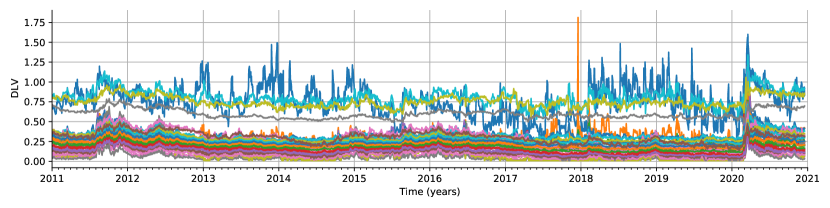
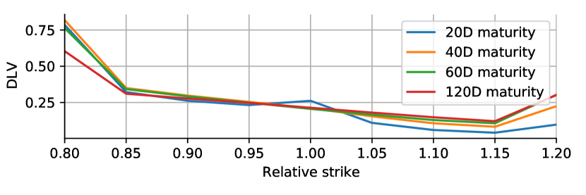
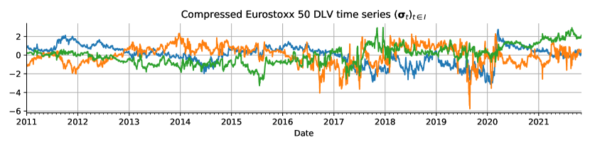
is therefore well-defined and bounded from below and above by and . Note that the mapping from the arbitrage-free surface to the DLVs is bijective. For illustration we display the DLVs of Eurostoxx 50 for the January 2011 to November 2021 in Figure 1 for the grid of maturities and relative strikes .
2.2 Stylized facts of spot and equity option markets
To assess the fidelity of a calibrated market simulator, we review the features of the spot and equity option market. Spot market dynamics have been extensively studied in the past. The most characteristic features of the spot market were summarised by [16] [16] and coined as stylized facts. We summarise the most prominent features of spot log-returns from [16] [16] as follows:
-
•
Fat tails: evaluation of the tails of the empirical unconditional return distribution indicates the presence of fat tails, i.e. power-law decay in the tail of the density.
-
•
No serial correlation: spot log-returns have close to zero serial autocorrelation, i.e. they are hard to predict linearly.
-
•
Volatility clusters: volatility tends to appear in clusters. Large absolute spot log-returns generally follow large absolute spot log-returns. This observation can be measured by computing the autocorrelations of absolute or squared spot log-returns.
-
•
Leverage effects: absolute spot log-returns and log-returns are negatively correlated: a large fall in spot levels causes an increase in volatility.
The empirical observations above influenced the design of stochastic volatility models in the past by incorporating these observed dynamics, such as leverage effects and volatility clustering, into the model (for example see the Heston model [29]).
Stylized facts of DLVs are discussed for the first time in this paper, but due to their local volatility inspired parametrisation are consistent with general observations of equity option volatility surfaces. We highlight the most important ones as follows:
- •
-
•
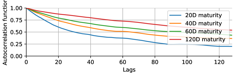
Persistence: DLVs have high serial autocorrelation and the autocorrelation for short-dated DLVs drops generally faster than for long-dated ones. Figure 4 displays the autocorrelation function for the first 128 lags for the ATM DLVs for maturities business days; again for the Eurostoxx 50 dataset.
-
•
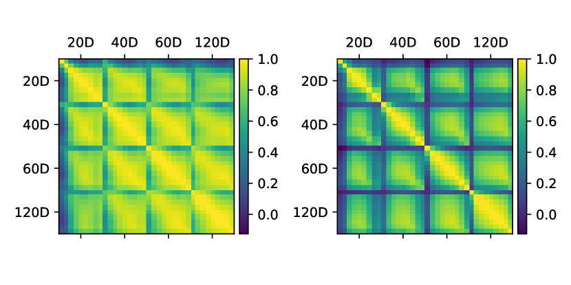
Cross-correlations: DLV strike-maturity pairs show high cross-correlation for proximate relative strikes and maturities. This is true for DLV levels as well as their returns (see Figure 2).
3 Literature overview on market simulation
The absence of large equity option market datasets on a daily time scale has created attention from academia and industry. Although past works have studied modeling the dynamics and stylized facts of asset returns through diffusions in order to calibrate models for pricing under a risk-neutral measure , they do not model the dynamics of the volatility surface under the real-world measure . Though traditional models can give an accurate fit of a single instance of the volatility surface they require constant day-to-day recalibration.
Most models that fall into this category are parametric models that describe a family of distributions. In the financial mathematics literature examples are the Black-Scholes [7], Heston [29], SABR [28] and rough volatility model [25]. While these SDE-type models are explainable they face a trade-off between complexity and tractability which may cause difficulties in calibration. At the same time, the less complex a model becomes the higher the probability of model misspecification. In this paper, we use normalizing flows as a universal approximator for estimating the conditional discrete-time dynamics of the market [24]. Our proposed market simulator, thus, is parametric in the sense that it describes a family of densities. However, through the high parametrisation of neural networks, our simulator is capable of universally approximating conditional densities such that the possibility of model misspecification is reduced111The generator formulation assumes a noise-state relationship. The incorporation of jumps is left as future work..
More recently, with increasing interest in generative modeling, the focus has shifted on calibrating nonparametric models under the physical measure . [2] introduced Sig-SDEs, a signature-based SDE-type model, for pricing and risk management. [11] proposed to combine signatures with autoencoders to generate realistic spot dynamics but require an accurate projection from signature to path space. Very recently, [15] introduced an arbitrage-free neural SDE model which guarantees no dynamic arbitrage and minimizes the chance of generating static arbitrage. Various other works, including our single asset market simulator [54], explored the application of GANs for simulating high-fidelity market data [18, 19, 34, 36, 40, 41, 47, 55].
Of the above mentioned works, our paper on simulating high-fidelity spot and equity option markets is most related to the work of [15] [15] but differs in a number of aspects. First, our study is performed on real-world datasets, whereas [15] perform their study on a 2-factor Heston stochastic local volatility (SLV) model [31]. Second, while [15] use a constrained PCA to find a linear call price basis for a lattice of call prices, we use an arbitrage-free parametrisation of a call price grid. This allows us to approximate the nonlinear pricing functional by the means of autoencoders [30] and enables us to learn efficient low-dimensional representations, whereas [15] need 3-factors to represent the ground truth 2-factor SLV model. Third, [15] enforce no dynamic arbitrage which is possible because they work under the risk-neutral measure . We do not impose this constraint since we work under the real-world measure which contains dynamic arbitrage. Last, our model is formulated in discrete-time whereas [15] calibrate a continuous-time neural SDE. While a continuous-time simulator generating intraday tick prices and volumes may allow for enhanced risk management, we believe that this is a separate problem and leave it as future research.
We emphasise that our approach of learning nonlinear and arbitrage-free representations of the volatility surface by means of autoencoders and DLVs is novel and allows us to calibrate the pricing functional of the underlying. While several works have studied the application of PCA [15, 16] and variational autoencoders [5, 42] for compression, these approaches are either limited by being linear, do not guarantee no static arbitrage, or cannot represent a rich family of call price surfaces.
We highlight that we are not the first to apply normalizing flows to the application of modeling time series [20] or conditional densities [48]. [20] proposed continuous-time flow processes (CTFP) by leveraging neural ODEs for modeling the densities of the continuous-time process. While the CTFP solves the problem of sampling stationary time series on a fixed time horizon it does not solve the stationarity problem on a general time horizon where the terminal time is variable as the flow cannot generalise and extrapolate the non-stationary dynamics of the Brownian motion. Since downstream algorithms require sampling from the market simulator from variable terminal time , we do not incorporate the continuous-time perspective.
4 Normalizing flows
Normalizing flows [22, 24, 43, 53] are a class of functions within the function space of neural networks which are differentiable and bijective, more commonly referred to as diffeomorphisms. In this section, we introduce the reader to the application of diffeomorphisms for modeling unconditional densities in subsection 4.1, discuss the existence of a diffeomorphism in subsection 4.2, how neural networks can be used to approximate bijective functions in subsection 4.3 and finally show how a network-based linear neural spline conditional on data can be constructed in subsection 4.4.
4.1 Modeling unconditional densities with normalizing flows
Let be a simple source density, such as a multivariate normal, defined on a source space , and a target density defined on a compact target space . Assume that the target density is unknown. In generative modeling, the goal is to approximate a parametrisable map to transform the source distribution such that the model density and the target density are close with respect to some metric. Let be a diffeomorphism and denote by the model density induced by . The density transformation theorem states that the density of admits the form
| (1) | ||||
| (2) |
where is the inverse, denotes the matrix determinant operator and denotes the Jacobian of
where we dropped the dependence on for legibility.
The tractability of the model density emerges as a great advantage as this property allows measuring the distance of the model and target density by employing -divergences [35] such as the Kullback-Leibler (KL) divergence. The KL-divergence of and is given as
| (3) | ||||
| (4) | ||||
| (5) |
Hence, when is available the KL-divergence can be evaluated numerically. However, in practice the target density is generally unknown and only a set of realizations sampled from the target density is available. Thus, the KL divergence in \tagform@5 cannot be computed explicitly. Instead the integral is approximated via Monte Carlo:
| (6) |
Remark 1 (-divergences).
The KL-divergence is a single instance of a more broader class of -divergences [35]. The reason for the KL-divergence’s popularity and application in this paper is that the diffeomorphism’s parameters only depend on the negative expected log-model density under the target density
Note that this makes it possible, as opposed to other -divergences, to approximate the -dependant integral of the KL-divergence via Monte Carlo without having prior knowledge of the target density.
Normalizing flows approximate diffeomorphisms by applying gradient descent to the MC-approximated KL-divergence:
4.2 Existence of a transport map
In the previous section we assumed that diffeomorphisms can be used to transform any source density to some target density. In general, this only holds when the source and target density have overlapping supports. To prove the existence of a diffeomorphism that can transport a source density to a target density we recall the notion of an increasing triangular map. A function is called triangular if for any the function only depends on inputs . Furthermore, we call a triangular map increasing if for any the function is monotonically increasing in . The following highly-celebrated result by [8] proved the existence of triangular maps for absolutely continuous Borel measures:
Theorem 1 ([8, Lemma 2.1]).
If and are absolutely continuous Borel probability measure on , then there exists a unique (up to null sets of ) increasing triangular map such that .222Here denotes the pushforward measure of which is defined for any Borel set as . The same holds over .
The ability to approximate arbitrarily complex increasing triangular maps and diffeomorphisms is the core field of research of normalizing flows.
Remark 2 (Model misspecification).
By constructing an algorithm that can approximate universally diffeomorphisms we leave the realm of quasi maximum likelihood estimation, since for any absolutely continuous source / target density pair there exists a parametrised diffeomorphism that can transform the source to the target density. Thus, model misspecification is not possible anymore.
4.3 Approximating diffeomorphisms with neural networks
In the previous two subsections, we assumed that the model density can be evaluated efficiently. However, this depends on the ability to compute the inverse and the matrix determinant of the Jacobian . In this subsection, we take a glance at the ideas that have been applied to approximate diffeomorphisms with neural networks such that both requirements on the map are fulfilled. We constrain ourselves to autoregressive flows and direct the reader to [44] for a more in-depth overview on normalizing flows.
Let be a diffeomorphism composed of diffeomorphisms
and denote by the -th successive composition / transformation and let denote the joint parameters. The log-determinant of the Jacobian of is given as
where and we dropped -dependence for legibility. Hence, for the computation of the determinant to be efficient the computation of the determinants of needs to be efficient. To realize this requirement, it makes sense to construct the diffeomorphisms to be sufficiently simple, but expressive enough to make universal.
4.4 Linear neural splines
In this subsection, we introduce linear neural splines [24]. Linear neural splines are a special instance of normalizing flows and will be used in section 5 to approximate the market simulator.
Neural splines follow the idea of approximating a diffeomorphism by constructing a triangular map. In the univariate case a neural spline degenerates to approximating the composition of the CDF of the source density and the inverse CDF of the target density.333Assume that the random variables and have CDFs respectively. Then the optimal diffeomorphism transforming the source to the target distribution is defined as . Therefore, assume that the neural spline was to model a -variate density defined on by pushing forward an absolutely continuous source density . We also assume that we were to model the component and let be a neural network with parameter space and output space where represents the number of knots used to define the spline. Furthermore, denote by the first components of the -variate vector and the output of the network. To construct the monotonically increasing spline the outputs need to be transformed such that they represent monotonically increasing coordinates in . For this purpose, let be the softmax function and the cumulative sum function which computes the successive cumulative sum. The spline’s -valued coordinates can be computed by applying the softmax and the cumulative sum function
Finally, we are able to define the neural spline as
Above we assumed that target density had support on the hypercube . Neural splines can be generalized to by applying an affine transformation to the coordinates and extrapolating the tail behaviour through predefined / extrapolated tails. Furthermore, generalisations of the here introduced linear spline construction have been introduced in [24] for monotonic rational-quadratic splines and in [23] for cubic splines.
5 Simulating single-asset spot and equity option markets with normalizing flows
After introducing spot and equity option markets and normalizing flows, we formally present in this section the proposed flow-based market simulator for a single underlying. The section is divided into four parts:
-
•
Subsection 5.1: nonlinear arbitrage-free compression of the call price surface,
-
•
Subsection 5.2: derivation of the market simulator objective,
-
•
Subsection 5.3: modifications to the simulator to guarantee the martingale property,
-
•
Subsection 5.4: numerical results demonstrating the performance of the calibrated Eurostoxx 50 market simulator.
Throughout this section, we denote by the time horizon, for by and the historical -dimensional grid of DLVs and the spot level respectively and for by the spot log-return.
5.1 Learning efficient arbitrage-free representations of the call price surface
DLV levels as well as their returns are highly correlated for proximate relative strikes and maturities (see Figure 2). Since our aim is to calibrate a market simulator from limited real-world market data it does not make sense to the full joint distribution of each DLV strike-maturity combination due to the curse of dimensionality [6]. We therefore reduce the dimensionality of the grid of DLVs using an autoencoder. Autoencoders are neural networks with a bottleneck structure that are trained to learn the identity mapping through a reconstruction error. The bottleneck structure forces the network to learn a low-dimensional encoding of the DLV grid. An autoencoder can be split up into two parts: an encoder function which compresses the grid and a decoder function reconstructing / decompressing the encoding.
The only requirement that needs to be satisfied in order to ensure no static arbitrage in the reconstructed call prices which we obtain from inverting the reconstructed DLVs (see subsection 2.1) is that the reconstructed DLVs are non-negative. We therefore preprocess DLVs to log-DLVs to ensure that the DLVs are non-negative and then standard scale them
where and is the component-wise empirical mean and standard deviation respectively and denotes component-wise division.
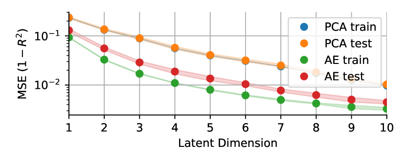
To demonstrate the efficacy of our DLV autoencoder approach we compare the autoencoder (AE) with a principal component analysis (PCA) (see [6, Chapter 12.1]) performed on the DLVs. We shuffle the preprocessed data via random permutations and then split the shuffled data into a train and test dataset ; where denotes the indices of the training set and the indices of the test. We retain of the data within the train dataset; are used in the test set. The autoencoder is implemented using the high-performance deep learning library pytorch [45, 46] and is trained using the Adam optimizer [32] with a learning rate of and DropOut [51] across all layers to mitigate overfitting. The loss function used is the mean-squared error (MSE), also known as the image loss or reconstruction error;
where denotes the -norm. Note that we scale the sum by the scalar constant so that the learning rate is invariant to a change in the size of the dataset or the DLV grid.
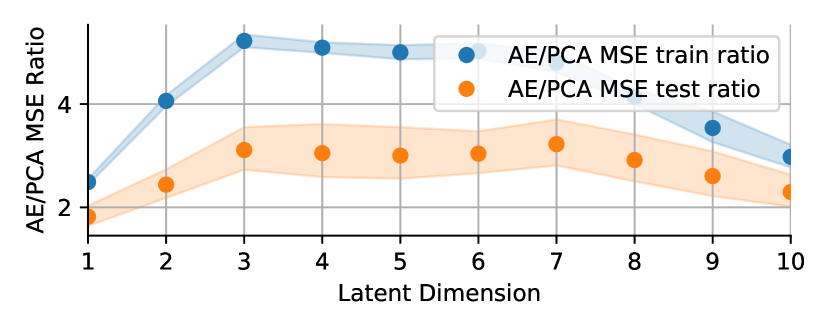
The above training procedure is performed across ten different seeds and latent dimensions one through ten. For each seed and latent dimension we store the MSE on the train and test set. The mean MSE obtained across all seeds for each individual latent dimension is reported in Table 1 and visualised additionally in Figure 6. The error bars around each mean MSE show the standard deviation of the MSEs obtained for each latent dimension to give a sense of the variation and reproducibility we obtained during training. Furthermore, we display the AE and PCA MSE ratio in Figure 6 which shows that in terms of the MSE the AE beats PCA by a factor of two to five on the train set and two to three on the test set highlighting the efficiency of the DLV-AE approach in contrast to a linear encoding. Figure 7 displays a three-dimensional encoding of the DLV grid obtained through a trained autoencoder.
| Latent dimension | 1 | 2 | 3 | 4 | 5 | 6 | 7 | 8 | 9 | 10 |
|---|---|---|---|---|---|---|---|---|---|---|
| AE train set | ||||||||||
| PCA train set | ||||||||||
| AE test set | ||||||||||
| PCA test set |
5.2 Derivation of the market simulator’s objective
In the last section, we addressed the curse of dimensionality by the means of a DLV-based autoencoder which is able to learn an efficient low-dimensional encoding of the call price surface while satisfying no static arbitrage in the reconstructed surface. In this section, we construct the market simulator and derive the objective function.
Assume that there is a calibrated encoder function that encodes the preprocessed DLV grid to the compressed space and denote the compressed process by . Furthermore, denote by for the market state. Our aim in this section is to calibrate a model density such that for any -lagged market states and next-day market state the target and model conditional densities and are close with respect to the Kullback-Leibler divergence.
Here, the conditional model density will be represented through a conditional normalizing flow where the flow will not only be parametrised by some parameter space but also by the past market states . Let
be such a function mapping the -lagged states to a diffeomorphism, i.e. for fixed the function is a diffeomorphism. Likewise to the unconditional case described in subsection 4.1 the model density conditional on can be expressed via the density transformation theorem
| (7) |
For calibration we use the expected conditional KL-divergence since our interest is to calibrate the conditional density not only for a single condition but across all possible past conditions weighted by their likelihood
In practice, due to the limited amount of market data, the ground truth density is not available. Instead only a realization exists. We therefore approximate the expected conditional KL-divergence via Monte Carlo:
| (8) |
where we dropped the constant term for legibility. Minimization of the objective is performed via gradient descent.
5.3 Addressing non-zero drift in generated spot prices
Conditional drift in the generated spot prices is the most obvious form of statistical arbitrage which can be exploited by a downstream algorithm such as Deep Hedging. If the spot drift conditional on is positive (negative) Deep Hedging will buy (sell) the underlying and make a profit in expectation. From daily spot data it’s hard to predict non-zero drift with any confidence. In our application, we do not want to be sensitive to drift. We therefore choose to ensure the martingale property when generating spot prices.
In order to satisfy the martingale property, we impose a normal distribution onto the generated log-returns
| (9) |
where denotes the spot market’s realized volatility and the map the realized volatility estimator; in our application a neural network. While we do not claim that the historical spot log-returns follow a normal distribution, the proposed constraint is a first step to generating realistic martingale dynamics containing e.g. stochastic volatility, and we leave it as future work to relax the constraint \tagform@9. Figure 8 illustrates the construction and design of the spot and equity option simulator where the transport map is defined as
for .
5.4 Numerical results: Eurostoxx 50
In this section, we present numerical results and demonstrate empirical evidence that the trained market simulator performs well on a real-world single asset dataset. We consider the Eurostoxx 50 from January 2011 to November 2021 which amount to a total of 2711 business days. The DLV grid will be defined for relative strikes and maturities ; here quoted in business days. Figure 1 displays the considered DLV time series.
Prior to calibrating the neural spline an autoencoder is trained as described in subsection 5.1 using a three-dimensional bottleneck. Figure 7 depicts the compressed state representation. Afterwards, the compressed representation is standard-scaled (z-transformed) and concatenated to the spot log-return series to obtain the market state time series ; where is the time set. Next, a rolling-window is applied to obtain the rolled time series containing the -lagged market states and the next-day market state. We chose for the lagged window as we observed that the second lag of the partial autocorrelation function of the compressed DLVs is non-neglibly far away from zero. The rolled series is then split into a train and test set via random permutations where of the data are held in the train set; the rest is retained in the test set.
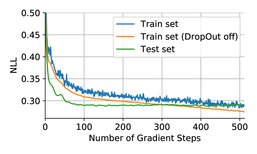
After compressing the DLVs and preparing the data the realized volatility estimator is trained to maximize the likelihood under the assumption that the spot log-return distribution follows a conditionally normal form \tagform@9. To approximate the realised volatility estimator we use a three layer neural network with 64 hidden dimensions and apply the exponential function as a last transformation to ensure that the predicted realized volatility is positive. The network is trained with the Adam optimizer, a learning rate of and DropOut to address overfitting. Figure 11 shows the decay of the loss function during the course of training. Early stopping is applied at the gradient step / iteration to stop the network from overfitting as at this point the test and train loss (when DropOut is turned off) intersect.
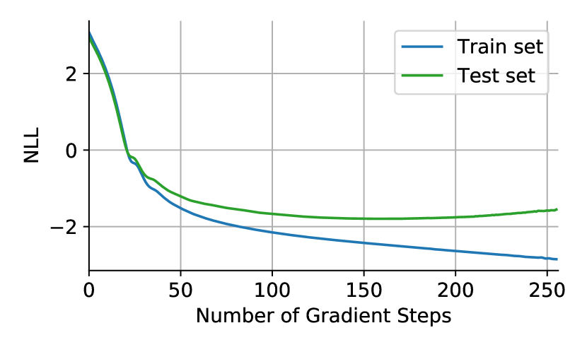
Next, the compressed state simulator map is calibrated through the NLL objective \tagform@8 and batch gradient descent. The flow is represented through three neural networks, each constructing a monotonically increasing linearly interpolated spline which will be used to transform the sampled Gaussians to the next-day compressed DLVs . Each network-based spline approximator will have three hidden layers with hidden dimensions. Furthermore, we use the Adam optimizer with a learning rate of for calibration. of the data is kept in the train set and the rest is used in the test set to assess whether the model is overfitting. Figure 11 shows the development of the NLL on the train (blue) and test set (green). We observed that the test set error stopped to decay at the iteration and applied early stopping there.
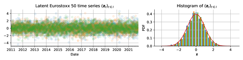
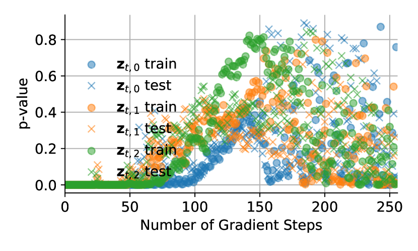
After training the full market simulator we measure the goodness of the fitted model. Evaluation is split into two parts: assessment of the latent time series and performance on distributional and dependency measures. The latent time series is computed by inverting the rolled time series . Figure 12 depicts the latent series as well as its empirical distribution. Visually, we can observe that the latent series resembles properties of a normally distributed i.i.d process. Furthermore, we can verify that the empirical probability density function (PDF) is close to the standard normal PDF (displayed in red in Figure 12). To further assess the proximity of the latent unconditional distribution to the standard normal we apply a Kolmogorov-Smirnov (KS) test [37] to each component individually and test whether we can reject the null hypothesis () that the samples were sampled from a standard normal distribution. Table 2 reports the -values obtained from the KS test and we conclude that we cannot reject at a (approximately) and confidence level on the train and test set respectively.
| Data set | Train set | Test set | ||||
|---|---|---|---|---|---|---|
| Latent component | 1 | 2 | 3 | 1 | 2 | 3 |
| KS -value | 0.2889 | 0.5624 | 0.7962 | 0.3335 | 0.2586 | 0.2898 |
During calibration we additionally tracked the -values on the train and test set depicted in Figure 11. Interestingly, the -values increase on the train and test set until the iteration and then start to rapidly decrease which coincides with the iteration range where the test set error starts to increase.
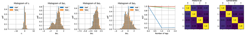
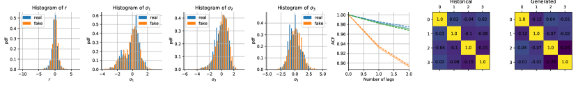
Our second assesment is based on the distributional and dependence properties on a short and large time horizon. We assess these properties individually on a varying time horizon as we want to determine whether short-term and the long-term invariant distribution of the simulator is proximate to the distribution of the data. For evaluation on the short time horizon we sample for each condition a total of of length
resulting in paths of length . We then assess the distributional and dependence properties of the level process in Figure 19 and return process , where is denotes the return of the compressed DLV grid, i.e. , in Figure 20. Figures 19 and 20 show from left to right histograms of the unconditional historical (blue) and generated (orange) distribution, as well as the autocorrelation function for the first lags and the historical and generated cross-correlation matrix. Visually, we can verify that the NLL objective used to calibrate the market simulator leads to a market simulator that approximates these statistical properties.
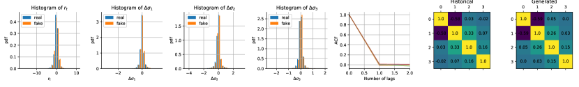
The same procedure as above is performed for evaluation of the long-term properties, however, here we sample for days and only retain the last days
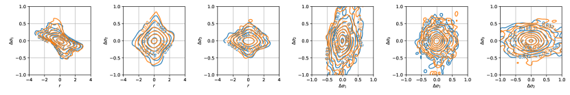
During simulation of long-term paths we noticed that approximately of the paths exploded and had to be discarded / rejected. We explain this observation in remark 3. Figure 13 and Figure 14 show the fitting performance of the level and return process respectively. Also here we observe that the fitting performance is accurate. Notably, we observe that the unconditional generated level distribution is slightly off from the historical, but still gives a good fit. Last, we also display the joint bi-variate distributions of the long-term return process in Figure 15 which shows that the calibrated flow gives an accurate fit.

Remark 3 (The extrapolation problem of network-based time series simulators).
During simulation of the long time series we observed that with a non-zero probability some of the paths diverged / exploded. This observation is plausible: the simulator may generate states that it was not trained on or states that are off the empirical manifold. Since neural networks are known not to genalise well to unknown data (here past conditions ) (see for example [3, Section 4.1]) it is natural, but highly unfavorable, to observe this phenomenon, as rejecting generated paths alters the distribution of the generated spot process causing it not to satisfy the martingale property which we wanted to guarantee by construction (see subsection 5.3). We believe that the extrapolation problem is challenging but essential for constructing high-fidelity market simulators and want to address it in future work. Last, we would like to note that this observation was not only made for our flow-based simulator but for any network-based simulator that was trained using adversarial training techniques [40, 54].
6 Multi-asset market simulation: sampling from joint distribution of the asset universe
After introducing the conditional spot and equity option market simulator for a single underlying, we cover in this section the topic of simulating multi-asset markets. Assume an -variate spot and equity option market and identify each underlying’s individual market state with a superscript, i.e. , where and denote the -th underyling’s spot log-return and compressed DLV grid respectively. Let be optimal simulators in the sense that for any asset the model densities are equal to the (unknown) target densities for any . Furthermore, denote by the joint market simulator which is defined for any joint -lagged market state as
where is the joint latent process where follows the simple source density which we assume to be the standard multivariate normal distribution .
Our aim in this section is to calibrate the joint distribution of the joint latent process in a scalable manner while not altering the conditional density of the individual simulators . We therefore assume for any joint -lagged market state that the joint density of the latent random variable is independent from the state
| () |
and refer to this as the static noise assumption. Although the noise distribution may be state-dependent, our aim in this paper is to find a fast and scalable calibration algorithm for correlating the market simulators and we leave it as future work to construct state-dependent joint densities in a scalable manner.

Under the static noise assumption it is sufficient to calibrate a copula [38] to capture the multi-asset’s joint distribution. For this purpose we propose to use a Gaussian copula to model the joint distribution. When specifying the Gaussian copula as the parametric family we assume that the joint latent process follows a normal distribution with covariance matrix where the covariance matrix satisfies the block structure
| (10) |
The covariance matrix can be estimated directly from the joint latent series
| (11) |
where denotes the sample mean and is used to denote the outer product. To ensure that the dynamics of each individual simulator are not changed through sampling of the Gaussian copula, we additionally enforce during estimation of that the blocks along the diagonal are equal to the identity matrix. Thus, if and is of the form \tagform@10, then the conditional model densities remain unchanged.
We benchmark the Gaussian copula against a more complicated flow-based model , as described in section 4, that will aim to transform a standard normal source distribution to the targeted distribution . It is important to note that while the flow is able to capture non-linear structure of the joint distribution of the joint latent time series, it also alters the marginal density resulting in a changed model density . While it is possible to account for this change in the marginal density, it is non-trivial to say how strong the effect will be on the calibrated joint density after such a correction.
6.1 Numerical results: Eurostoxx 50 and S&P 500
Above we motivated the use of copulas for modeling the joint latent distribution. In this section, we benchmark the Gaussian copula against a flow-based calibration. We consider the Eurostoxx 50 as well as the S&P 500 from January 2011 to November 2021 for the same DLV grid we considered in subsection 5.4, i.e. maturities (quoted in business days) and relative strikes . Prior to calibration of the joint latent distribution we proceed as in subsection 5.1 and subsection 5.4 to calibrate the autoencoder with a three-dimensional bottleneck, realized volatility estimator and compressed state simulator map for each underlying individually.
After calibration of the market simulators we compute the latent process by inverting the flow. We then estimate the covariance matrix through \tagform@11 and impose the block structure as described in \tagform@10. Afterwards, we train the unconditional flow. Here, the flow will be represented by a three layer network with 64 hidden dimensions. Similar to the procedure described in subsection 5.4 the data is split into a train and test set, the Adam optimizer is used with a learning rate of and DropOut is used.
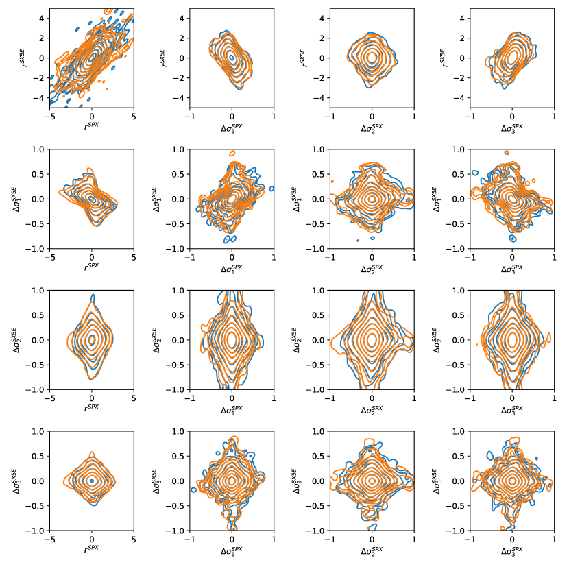
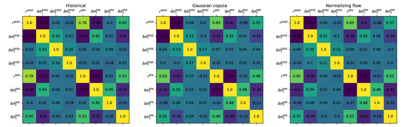
Afterwards, evaluate the fitting performance and sample paths on a short time horizon by using the sampling scheme described in subsection 5.4. To assess the fitting performance we perform a kernel density estimate on the bivariate joint distributions. The kernel estimate of the historical (blue) and generated (orange) return distribution is depicted in Figure 16 for the Gaussian copula and in Figure 17 for the flow-based copula. Furthermore, Figure 18 shows the cross-correlation matrix of the return distribution of the historical, Gaussian copula simulated and flow simulated paths. Comparing both visually the kernel density estimate of the Gaussian copula and the normalizing flow it is not apparent which of the two outperforms the other. A similar claim can be made when looking at the cross-correlation matrices as both matrices do not deviate strongly from another. Since the Gaussian copula ensures that the dynamics of the individual market simulators remain unchanged, we conclude in this numerical example that the Gaussian copula is more favorable than the flow-based calibration.
7 Conclusion and future research
In this paper, we presented formally a novel spot and equity option market simulator for a single underlying by utilizing normalizing flows. To overcome the curse of dimensionality of high-dimensional call price lattices we introduced an autoencoder which was able to learn efficient low-dimensional representations while maintaining no static arbitrage in the reconstructed surface by construction. We then introduced a fast and scalable method for calibrating the joint distribution of multiple independent simulators that were calibrated on distinct underlyings. We end this paper with future avenues of research / work.
Extrapolation problem
In subsection 5.4, we observed that with non-zero probability paths had to be rejected due to path explosions. Unfavorably, this has an effect on the generated spot distribution causing it to not satisfy the martingal property. While it is difficult to discover a regularization method that counteracts such explosions we find it to be a central research topic and want to advance this area with future work.
Realized volatility
We assumed in subsection 5.3 that realized volatility is a function of past market states. This estimator can be improved by simply replacing it through an estimator that estimates realized volatility from intraday prices / tick data. Furthermore, the market simulator can be improved by augmenting the market state through the realized volatilty estimate such that the dynamics of are modeled within the market simulator.
High-fidelity conditional spot distributions
To ensure the martingale property in the generated spot distribution a normal form \tagform@9 was imposed on the log-returns distribution in subsection 5.3. In general, the constraint is restrictive as it cannot capture features such as the skew and tail of the historical distribution. We believe it is fruitful to incorporate jump processes for modeling the generated spot distribution to more accurately capture tails and generalise the normal form, perhaps through a normalizing flow-based construction which satisfies the martingale property.
References
- [1] Martin Arjovsky, Soumith Chintala and Léon Bottou “Wasserstein generative adversarial networks” In International conference on machine learning, 2017, pp. 214–223 PMLR
- [2] Imanol Perez Arribas, Cristopher Salvi and Lukasz Szpruch “Sig-SDEs model for quantitative finance”, 2020 arXiv:2006.00218 [q-fin.CP]
- [3] Georgios Arvanitidis, Lars Kai Hansen and Søren Hauberg “Latent space oddity: on the curvature of deep generative models” In arXiv preprint arXiv:1710.11379, 2017
- [4] Samuel Assefa “Generating synthetic data in finance: opportunities, challenges and pitfalls” In Challenges and Pitfalls (June 23, 2020), 2020
- [5] Maxime Bergeron, Nicholas Fung, John Hull and Zissis Poulos “Variational Autoencoders: A Hands-Off Approach to Volatility”, 2021 arXiv:2102.03945 [q-fin.CP]
- [6] Christopher M Bishop “Pattern recognition” In Machine learning 128.9, 2006
- [7] Fischer Black and Myron Scholes “The Pricing of Options and Corporate Liabilities” In Journal of Political Economy 81.3 University of Chicago Press, 1973, pp. 637–654 URL: http://www.jstor.org/stable/1831029
- [8] Vladimir Igorevich Bogachev, Aleksandr Viktorovich Kolesnikov and Kirill Vladimirovich Medvedev “Triangular transformations of measures” In Sbornik: Mathematics 196.3 IOP Publishing, 2005, pp. 309
- [9] Hans Buehler and Evgeny Ryskin “Discrete local volatility for large time steps (extended version)” In Available at SSRN 2642630, 2017
- [10] Hans Buehler and Evgeny Ryskin “Discrete Local Volatility for Large Time Steps (Short Version)” In Available at SSRN 2783409, 2018
- [11] Hans Buehler et al. “A Data-driven Market Simulator for Small Data Environments”, 2020 arXiv:2006.14498 [q-fin.ST]
- [12] Hans Buehler, Lukas Gonon, Josef Teichmann and Ben Wood “Deep Hedging” In Quantitative Finance 19.8 Taylor & Francis, 2019, pp. 1271–1291
- [13] Hans Buehler et al. “Deep hedging: hedging derivatives under generic market frictions using reinforcement learning” In Swiss Finance Institute Research Paper, 2019
- [14] Hans Buehler, Phillip Murray, Mikko S. Pakkanen and Ben Wood “Deep Hedging: Learning to Remove the Drift under Trading Frictions with Minimal Equivalent Near-Martingale Measures”, 2021 arXiv:2111.07844 [q-fin.CP]
- [15] Samuel N. Cohen, Christoph Reisinger and Sheng Wang “Arbitrage-free neural-SDE market models”, 2021 arXiv:2105.11053 [q-fin.CP]
- [16] Rama Cont “Empirical properties of asset returns: stylized facts and statistical issues” In Quantitative finance 1.2 IOP Publishing, 2001, pp. 223
- [17] Christa Cuchiero, Wahid Khosrawi and Josef Teichmann “A generative adversarial network approach to calibration of local stochastic volatility models” In Risks 8.4 Multidisciplinary Digital Publishing Institute, 2020, pp. 101
- [18] Fernando De Meer Pardo and Rafael Cobo López “Mitigating overfitting on financial datasets with generative adversarial networks” In The Journal of Financial Data Science 2.1 Institutional Investor Journals Umbrella, 2020, pp. 76–85
- [19] Fernando De Meer Pardo, Peter Schwendner and Marcus Wunsch “Tackling the exponential scaling of signature-based GANs for high-dimensional financial time series generation” In Available at SSRN 3942764, 2021
- [20] Ruizhi Deng et al. “Modeling Continuous Stochastic Processes with Dynamic Normalizing Flows”, 2021 arXiv:2002.10516 [cs.LG]
- [21] Yue Deng et al. “Deep direct reinforcement learning for financial signal representation and trading” In IEEE transactions on neural networks and learning systems 28.3 IEEE, 2016, pp. 653–664
- [22] Laurent Dinh, Jascha Sohl-Dickstein and Samy Bengio “Density estimation using real nvp” In arXiv preprint arXiv:1605.08803, 2016
- [23] Conor Durkan, Artur Bekasov, Iain Murray and George Papamakarios “Cubic-spline flows” In arXiv preprint arXiv:1906.02145, 2019
- [24] Conor Durkan, Artur Bekasov, Iain Murray and George Papamakarios “Neural spline flows” In Advances in Neural Information Processing Systems 32, 2019, pp. 7511–7522
- [25] Jim Gatheral, Thibault Jaisson and Mathieu Rosenbaum “Volatility is rough” In Quantitative finance 18.6 Taylor & Francis, 2018, pp. 933–949
- [26] Ian Goodfellow et al. “Generative adversarial nets” In Advances in neural information processing systems 27, 2014
- [27] Ishaan Gulrajani et al. “Improved training of wasserstein gans” In arXiv preprint arXiv:1704.00028, 2017
- [28] Patrick S Hagan, Deep Kumar, Andrew S Lesniewski and Diana E Woodward “Managing smile risk” In The Best of Wilmott 1, 2002, pp. 249–296
- [29] Steven L Heston “A closed-form solution for options with stochastic volatility with applications to bond and currency options” In The review of financial studies 6.2 Oxford University Press, 1993, pp. 327–343
- [30] Geoffrey E Hinton and Ruslan R Salakhutdinov “Reducing the dimensionality of data with neural networks” In science 313.5786 American Association for the Advancement of Science, 2006, pp. 504–507
- [31] Michal Jex, Richard C. Henderson and Desheng Wang “Pricing Exotics Under the Smile”, 1999
- [32] Diederik P Kingma and Jimmy Ba “Adam: A method for stochastic optimization” In arXiv preprint arXiv:1412.6980, 2014
- [33] Alexei Kondratyev and Christian Schwarz “The market generator” In Available at SSRN 3384948, 2019
- [34] Adriano Koshiyama, Nick Firoozye and Philip Treleaven “Generative adversarial networks for financial trading strategies fine-tuning and combination” In Quantitative Finance 0.0 Routledge, 2020, pp. 1–17 DOI: 10.1080/14697688.2020.1790635
- [35] Friedrich Liese and Igor Vajda “On divergences and informations in statistics and information theory” In IEEE Transactions on Information Theory 52.10 IEEE, 2006, pp. 4394–4412
- [36] Gautier Marti “CORRGAN: Sampling Realistic Financial Correlation Matrices Using Generative Adversarial Networks” In ICASSP 2020 - 2020 IEEE International Conference on Acoustics, Speech and Signal Processing (ICASSP) IEEE, 2020 DOI: 10.1109/icassp40776.2020.9053276
- [37] Frank J Massey Jr “The Kolmogorov-Smirnov test for goodness of fit” In Journal of the American statistical Association 46.253 Taylor & Francis, 1951, pp. 68–78
- [38] Roger B Nelsen “An introduction to copulas” Springer Science & Business Media, 2007
- [39] Yuriy Nevmyvaka, Yi Feng and Michael Kearns “Reinforcement learning for optimized trade execution” In Proceedings of the 23rd international conference on Machine learning, 2006, pp. 673–680
- [40] Hao Ni et al. “Conditional Sig-Wasserstein GANs for Time Series Generation”, 2020 arXiv:2006.05421 [cs.LG]
- [41] Hao Ni et al. “Sig-Wasserstein GANs for Time Series Generation”, 2021 arXiv:2111.01207 [cs.LG]
- [42] Brian Ning, Sebastian Jaimungal, Xiaorong Zhang and Maxime Bergeron “Arbitrage-Free Implied Volatility Surface Generation with Variational Autoencoders”, 2021 arXiv:2108.04941 [q-fin.MF]
- [43] George Papamakarios, Theo Pavlakou and Iain Murray “Masked autoregressive flow for density estimation” In arXiv preprint arXiv:1705.07057, 2017
- [44] George Papamakarios et al. “Normalizing flows for probabilistic modeling and inference” In arXiv preprint arXiv:1912.02762, 2019
- [45] Adam Paszke et al. “Automatic differentiation in PyTorch” In NIPS-W, 2017
- [46] Adam Paszke et al. “PyTorch: An Imperative Style, High-Performance Deep Learning Library” In Advances in Neural Information Processing Systems 32 Curran Associates, Inc., 2019, pp. 8024–8035 URL: http://papers.neurips.cc/paper/9015-pytorch-an-imperative-style-high-performance-deep-learning-library.pdf
- [47] Jorino Rhijn, Cornelis W Oosterlee, Lech A Grzelak and Shuaiqiang Liu “Monte Carlo Simulation of SDEs using GANs” In arXiv preprint arXiv:2104.01437, 2021
- [48] Jonas Rothfuss et al. “Noise Regularization for Conditional Density Estimation”, 2020 arXiv:1907.08982 [stat.ML]
- [49] Johannes Ruf and Weiguan Wang “Neural networks for option pricing and hedging: a literature review” In Journal of Computational Finance, Forthcoming, 2020
- [50] Martin Schweizer and Johannes Wissel “Arbitrage-free market models for option prices: The multi-strike case” In Finance and Stochastics 12.4 Springer, 2008, pp. 469–505
- [51] Nitish Srivastava et al. “Dropout: A Simple Way to Prevent Neural Networks from Overfitting” In Journal of Machine Learning Research 15.56, 2014, pp. 1929–1958 URL: http://jmlr.org/papers/v15/srivastava14a.html
- [52] Richard S Sutton and Andrew G Barto “Reinforcement learning: An introduction” MIT press, 2018
- [53] Antoine Wehenkel and Gilles Louppe “Unconstrained monotonic neural networks” In Advances in Neural Information Processing Systems 32, 2019, pp. 1545–1555
- [54] Magnus Wiese, Lianjun Bai, Ben Wood and Hans Buehler “Deep hedging: learning to simulate equity option markets” In Available at SSRN 3470756, 2019
- [55] Magnus Wiese, Robert Knobloch, Ralf Korn and Peter Kretschmer “Quant GANs: deep generation of financial time series” In Quantitative Finance 20.9 Informa UK Limited, 2020, pp. 1419–1440 DOI: 10.1080/14697688.2020.1730426
Appendix A Disclosure
Opinions and estimates constitute our judgement as of the date of this Material, are for informational purposes only and are subject to change without notice. It is not a research report and is not intended as such. Past performance is not indicative of future results. This Material is not the product of J.P. Morgan’s Research Department and therefore, has not been prepared in accordance with legal requirements to promote the independence of research, including but not limited to, the prohibition on the dealing ahead of the dissemination of investment research. This Material is not intended as research, a recommendation, advice, offer or solicitation for the purchase or sale of any financial product or service, or to be used in any way for evaluating the merits of participating in any transaction. Please consult your own advisors regarding legal, tax, accounting or any other aspects including suitability implications for your particular circumstances. J.P. Morgan disclaims any responsibility or liability whatsoever for the quality, accuracy or completeness of the information herein, and for any reliance on, or use of this material in any way. Important disclosures at: www.jpmorgan.com/disclosures.
Appendix B Further numerical results