A Survey of Unsupervised Domain Adaptation for Visual Recognition

Abstract

While huge volumes of unlabeled data are generated and made available in many domains, the demand for automated understanding of visual data is higher than ever before. Most existing machine learning models typically rely on massive amounts of labeled training data to achieve high performance. Unfortunately, such a requirement cannot be met in real-world applications. The number of labels is limited and manually annotating data is expensive and time-consuming. It is often necessary to transfer knowledge from an existing labeled domain to a new domain. However, model performance degrades because of the differences between domains (domain shift or dataset bias). To overcome the burden of annotation, Domain Adaptation (DA) aims to mitigate the domain shift problem when transferring knowledge from one domain into another similar but different domain. Unsupervised DA (UDA) deals with a labeled source domain and an unlabeled target domain. The principal objective of UDA is to reduce the domain discrepancy between the labeled source data and unlabeled target data and to learn domain-invariant representations across the two domains during training. In this paper, we first define UDA problem. Secondly, we overview the state-of-the-art methods for different categories of UDA from both traditional methods and deep learning based methods. Finally, we collect frequently used benchmark datasets and report results of the state-of-the-art methods of UDA on visual recognition problem.

1 Introduction

In this era of big data, huge amounts of text, images, voices, and other types of data are produced. Industry and the research community have great demand for automatic classification, segmentation, and regression for multimedia data chen2018zero ; long2014transfer . Supervised learning is one of the most prevalent types of machine learning and has enjoyed much success across diverse application areas. In recent years, we have witnessed the great success of deep neural networks in some standard benchmarks such as ImageNet deng2009imagenet and CIFAR-10 krizhevsky2010convolutional . However, in the real world, we often have a serious problem that lacks labeled data for training. It is known that training and updating of the machine learning model depends on data annotation. Also, the high performance of machine learning models depends on the existence of massive labeled training data. Unfortunately, such a requirement cannot be met in many real scenarios with limited or no labels of collected data. Also, a major assumption is that the training and testing data have identical distributions. Such an assumption can be easily distorted if the background, quality, or shape deformation are different across the domains. In addition, it is often time-consuming and expensive to manually annotate data. This brings challenges to properly train and update machine learning models. As a result, some application areas have not been well developed due to insufficient labeled data for training. Therefore, it is often necessary to transfer knowledge from an existing labeled domain to a similar but different domain with limited or no labels.

However, due to the phenomenon of data bias or domain shift pan2010survey (when the target distribution, from which the test images are sampled, is different from the training source distribution), machine learning models do not generalize well from an existing domain to a novel unlabeled domain. For traditional machine learning approaches, we usually assume that training data (source domain) and test data (target domain) are from the same distribution, and models are optimized from training data to directly apply in test data for prediction. The differences between training and test data are omitted. However, there are often differences between the source and target domains, and traditional approaches have lower performance if there is a domain shift issue. It is hence important to mitigate the domain shift problem to improve model performance across different domains.

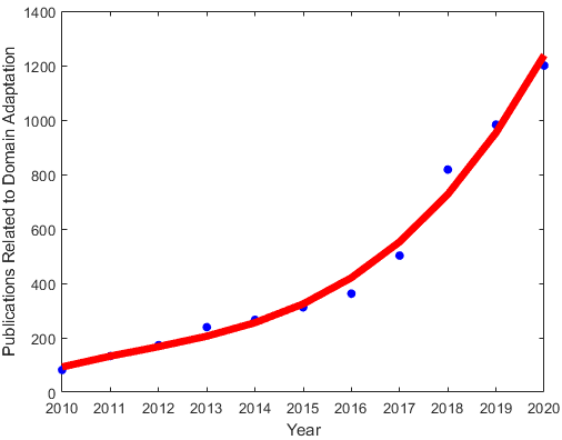
Domain adaptation (DA) is one of the special settings of transfer learning (TL), which aims to leverage knowledge from an abundant labeled source domain to learn an effective predictor for the target domain with limited or no labels while mitigating the domain shift problem. In recent years, DA keeps gaining attention in the computer vision field, as shown in Fig. 1. More and more DA related papers are published every year, which shows the importance of applications of DA. There are three types of DA (supervised, semi-supervised, and unsupervised DA), which depend on the number of labels in the target domain. For supervised DA, all target data labels are available. For semi-supervised DA, a portion of target data labels are available. For unsupervised domain adaptation (UDA), there is no label for the target domain. To circumvent the limitations posed by insufficient annotation, techniques combine the labeled source domain with unlabeled samples from the target domain. In addition, the number of categories of source and target domains are the same in UDA, which is also called closed set domain adaptation.

Figure 1: The popularity of domain adaptation. Statistics is from searching key word “domain adaptation” on Google Scholar (rough estimation, image from zhang2021unsupervised ).

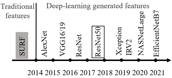
Existing domain adaptation methods assume that the data distributions of the source and target domains are different, but share the same label space. Traditional DA methods highly depend on the extracted features from raw images. With the development of deep neural networks, researchers are utilizing higher performance deep features (e.g., AlexNet krizhevsky2012imagenet , ResNet50 long2017deep , Xception zhang2019transductive , InceptionResNetv2 zhang2019modified ) instead of lower-level SURF features. However, the predictive accuracy of traditional methods is affected by the quality of the extracted features from deep neural networks zhang2020impact . Recently, deep neural network methods witness great success in domain adaptation problems. Especially, adversarial learning shows its power in embedding in deep neural networks to learn feature representations to minimize the discrepancy between the source and target domains tzeng2017adversarial ; liu2019transferable . However, it narrowly focuses on improving existing solutions from the source domain to the target domain, while structure information from target samples is hard to preserve. Also, it is difficult to remove noisily predicted labels in the target domain.

There have been developed several surveys on the TL and DA over the past fewer years pan2010survey ; shao2015transfer ; day2017survey ; patel2015visual ; zhang2017transfer ; csurka2017domain ; wang2018deep . Pan and Yang pan2010survey were the first to categorize TL under three settings: inductive TL, transductive TL, and unsupervised TL. Their focus is on the homogeneous feature spaces. Shao et al. shao2015transfer considered TL techniques for transferring knowledge of feature-representation level and classifier-level. Patel et al. patel2015visual only focused on DA as a special case of TL. Day and Khoshgoftaar day2017survey discussed heterogeneous TL in different settings. Zhang et al. zhang2017transfer summarized different transferring criteria based on concepts of DA. In general, these five surveys only covered models on traditional TL or DA. Later, Csurka csurka2017domain analyzed the state-of-the-art traditional DA methods and categorized the deep DA method. However, Csurka’s work discussed a few deep DA methods. Wang and Deng wang2018deep then classified the Deep DA into three groups: discrepancy based, adversarial based and reconstruction based methods based on Csurka’s work. However, they did not provide information regarding traditional methods.

In this paper, we mainly focus on the domain adaptation on image recognition tasks. The contributions of this survey are as follows. (i) We present a taxonomy of different DA using traditional and deep learning based methods. (ii) We are the first who study the traditional techniques in three different settings: feature selection, distribution adaptation, and subspace learning. (iii) We also discuss the deep learning based methods from discrepancy-based, adversarial-based, pseudo-labeling-based, reconstruction-based, representation-based, and attention-based methods. (iv) We collect several benchmark datasets, which is widely used in UDA and report results of state-of-the-art methods.

The rest of the paper is organized as follows: In Sections 2 and 3, we introduce the notations and generalization bound of DA problem. In Section 4, we review the traditional methods of UDA. In Section 5, we describe deep DA methods for image recognition. In Section 6, we list the benchmark datasets for DA and report the accuracy of state-of-the-art methods.

2 Notation

In this section, we formally define the notation in domain adaptation. A domain $\mathcal{D}$ consists of a feature space $\mathcal{X}$ by considering the marginal probability $P(\mathcal{X})$, and the task is defined by the label space $\mathcal{Y}$. The conditional distribution is $P(\mathcal{Y}|\mathcal{X})$, and the joint distribution is denoted as $P(\mathcal{X},\mathcal{Y})$.

When considering unsupervised domain adaptation in classification, there is a source domain $\mathcal{D_{S}}=\{\mathcal{X}_{\mathcal{S}}^{i},\mathcal{Y}_{\mathcal{S}}^{i}\}_{i=1}^{\mathcal{N}_{\mathcal{S}}}$ of $\mathcal{N}_{\mathcal{S}}$ labeled samples in $C$ categories and a target domain $\mathcal{D_{T}}=\{\mathcal{X}_{\mathcal{T}}^{j}\}_{j=1}^{\mathcal{N}_{\mathcal{T}}}$ of $\mathcal{N}_{\mathcal{T}}$ samples without any labels ($\mathcal{Y}_{\mathcal{T}}$ is unknown), also in $C$ categories. The samples $\mathcal{X_{S}}$ and $\mathcal{X_{T}}$ obey the marginal distribution of $P(\mathcal{X_{S}})$ and $P({\mathcal{X_{T}}})$. The conditional distributions of the two domains are denoted as $P(\mathcal{Y_{S}}|\mathcal{X_{S}})$ and $P(\mathcal{Y_{T}}|\mathcal{X_{T}})$, respectively. Due to the difference of the two domains, the distributions are assumed to be different, i.e., $P(\mathcal{X_{S}})\neq P({\mathcal{X_{T}}})$ and $P(\mathcal{Y_{S}}|\mathcal{X_{S}})\neq P(\mathcal{Y_{T}}|\mathcal{X_{T}})$. The goal for UDA is to learn a classifier with lower generalization error in the target domain by mitigating the domain discrepancy.

Figure 2: Taxonomy of unsupervised domain adaptation for image classification task (image adapted from zhang2021unsupervised ).

3 Generalization Bound for Domain Adaptation

Before discussing the domain adaptation methods, we first show the learning theory from Ben-David et al. ben2010theory to estimate the error bound of DA. It indicates that the target domain error can be minimized via bounding the source domain error and the discrepancy between them. Differing from most conventional machine learning methods, the domain adaptation approaches not only optimize the model with the source domain, but also consider the target data and reduce the discrepancy between them in the following Theorem.

Theorem 1 Let $\mathcal{H}$ be a hypothesis space. Given two domains $\mathcal{D_{S}}$ and $\mathcal{D_{T}}$, we have

$$\forall h\in\mathcal{H},\ R_{\mathcal{T}}(h) \leq R_{\mathcal{S}}(h)+d_{\mathcal{H}\Delta\mathcal{H}}(\mathcal{D_{S}},\mathcal{D_{T}})+\beta,$$

where $R_{\mathcal{S}}(h)$ and $R_{\mathcal{T}}(h)$ represent the source and target domain error, respectively. $d_{\mathcal{H}\Delta\mathcal{H}}$ is the discrepancy distance between two distributions $\mathcal{D_{S}}$ and $\mathcal{D_{T}}$ w.r.t. a hypothesis set $\mathcal{H}$. $\beta=\operatorname*{arg\,min}_{h\in\mathcal{H}}R_{\mathcal{S}}(h^{*},f_{\mathcal{S}})+R_{\mathcal{T}}(h^{*},f_{\mathcal{T}})$ where $f_{\mathcal{S}}$ and $f_{\mathcal{T}}$ are the label functions of the source and target domains, which can be determined by $\mathcal{Y_{S}}$ and pseudo target domain labels. $h^{*}$ is the ideal hypothesis and $\beta$ is the shared error and is expected to be negligibly small and can be disregarded.

Recall that $R_{\mathcal{S}}(h)$ can be minimized via training the labeled source domain. Existing DA models always aim to find a minimal $d_{\mathcal{H}\Delta\mathcal{H}}(\mathcal{D_{S}},\mathcal{D_{T}})$ to pursue a lower generalization bound of $R_{\mathcal{T}}(h)$.

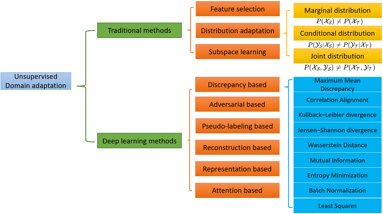
According to the similarities and differences between feature space and label space, the DA can be classified into two categories: homogeneous DA and heterogeneous DA. In homogeneous DA, the feature space is the same ($\mathcal{F_{S}}=\mathcal{F_{T}}$) with the same feature dimensionality ($d_{\mathcal{S}}=d_{\mathcal{T}}$). In heterogeneous DA ($\mathcal{F_{S}}\neq\mathcal{F_{T}}$), the feature dimensionality is different ($d_{\mathcal{S}}\neq d_{\mathcal{T}}$). In this paper, we will mainly discuss homogeneous DA and focus on the most challenges of unsupervised DA. In Secs. 4 and 5, we introduce a taxonomy of unsupervised domain adaptation for image classification task in two tracks: traditional methods and deep learning-based methods as shown in Fig. 2.

4 Traditional methods

In this section, we review traditional DA methods, which rely on extracted features from raw images. As shown in Fig. 2, we classify traditional DA methods into three sub-groups: feature selection, distribution adaptation, and subspace learning. For feature selection methods, we first learn a method to represent images, and we assume that the source and target domains share similarities in the features. Our goal is to select these features that are shared between the two domains. For distribution adaptation, we assume that the distributions of the source domain and target domain are different but share similarity, and we aim to align the distributions between the source domain and the target domain. For subspace learning, we assume that there is a shared subspace (a lower-dimensional representation) between two domains, and domain shift can be minimized in such a common subspace.

Figure 3: Frequently used image feature types for DA, while ResNet50 is the most frequently used deep network for feature extraction. IRV2: InceptionResNetv2. The shading SURF is traditional feature (image from zhang2021unsupervised ).

4.1 Feature selection methods

The first step for visual recognition is to find a proper way to represent images. In recent decades, with the emergence of deep networks, the feature representation of images has changed rapidly. As shown in Fig. 3, speeded up robust features (SURF) is one of the most popular extracted features for visual recognition before the deep features. It is a fast and robust algorithm for local, similarity invariant representation, and comparison of images feature bay2006surf . However, SURF can only detect some points, but not all important features. After the emergence of different ImageNet-trained deep models, their deep features have been widely used in the field of computer vision as shown in Fig. 3. The underlying assumption of the feature selection method is that both the source domain and the target domain contain at least some common features. The goal of this kind of method is to select these shared features through a machine learning method and then build models based on these features.

Structural correspondence learning (SCL) blitzer2006domain is one of the most representative models to find the common features of both domains. These common features are named as Pivot features, which refer to the words that frequently appear in different domains in text classification. Due to the stability of these features, they can be used as the bridge to transfer knowledge. It has three steps. 1) Feature Selection: SCL first obtains the pivot features; 2) Mapping Learning: the pivot features are utilized to find a low-dimensional common latent feature space; 3) Feature Stacking: a new feature representation is constructed by feature augmentation.

Figure 4: The scheme of Pivot feature in feature selection methods (image from blitzer2006domain ).

Esmat et al. rashedi2013simultaneous proposed a mixed gravitational search algorithm (MGSA) to reduce the semantic gap between low-level visual features and high-level semantics through simultaneous feature adaptation and feature selection. Later, feature selection and structure preservation (FFSL) li2016joint smoothly integrated structure preservation and feature selection into a unified optimization problem. They first selected relevant features across two domains and then utilized a nearest neighbor graph and a representation matrix to preserve the geometric structure. Also, there are extended works to incorporate other techniques. Gu et al. gu2011joint proposed a joint feature selection and a subspace learning model to unify feature selection and subspace learning in a framework. Transfer Joint Matching (TJM) long2014transfer , simultaneously adapted marginal distribution and performed source domain sampling selection during the process of optimizing an objective function. Combining deep features with traditional methods has also been explored zhang2018automated ; zhang2019regressive ; wu2020mixing , Zhang et al. investigated how different pre-trained ImageNet models affect transfer accuracy on domain adaptation problems zhang2020impact . They found that features from a better ImageNet model can improve the performance of domain adaptation. This observation was further validated by their later work zhang2021efficient .

Figure 5: An example of different types of distribution alignment. Type I: marginal distribution; Type II: conditional distribution; Type III: joint distribution (including aligning both I and II). Black line: classifier (image from zhang2021unsupervised ).

4.2 Distribution adaptation methods

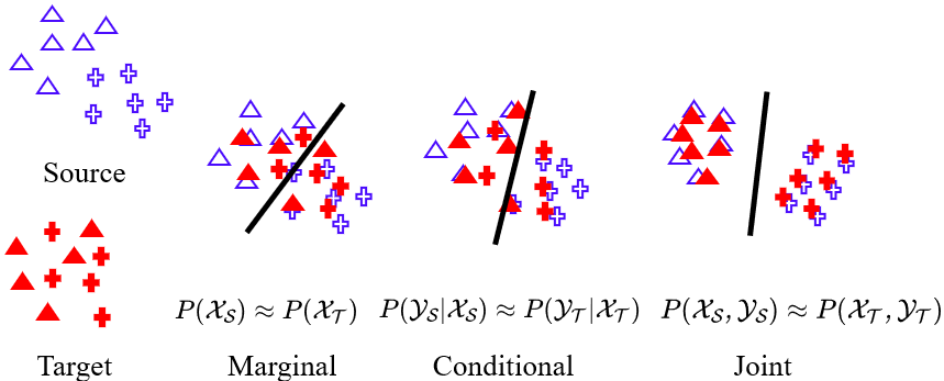
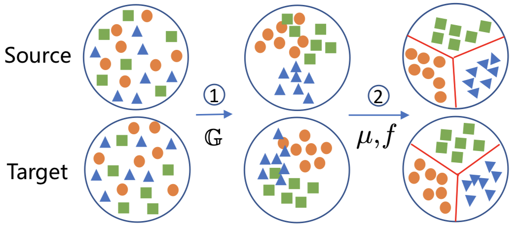
Distribution adaptation methods can be classified into three categories: marginal distribution adaptation ($P(\mathcal{X_{S}})\neq$ $P(\mathcal{X_{T}})$), conditional distribution adaptation ($P(\mathcal{Y_{S}}|\mathcal{X_{S}})\neq$ $P(\mathcal{Y_{T}}|\mathcal{X_{T}})$) and joint distribution adaptation ($P(\mathcal{X_{S}},\mathcal{Y_{S}})\neq P(\mathcal{X_{T}},\mathcal{Y_{T}})$). Therefore, many methods aim to minimize domain shift from these three directions to make these distributions are similar to each other across different domains. Fig. 5 illustrates the different priorities of distribution, Type I first aligns the marginal distribution and type II first aligns the conditional distribution, and type III aligns the marginal and conditional distribution together.

4.2.1 Marginal distribution adaptation

In this setting, it assumes that the marginal distributions between the two domains are different ($P(\mathcal{X_{S})}\neq$ $P\mathcal{(X_{T}})$), which should be aligned first. This pattern is shown as the marginal distribution alignment in Fig. 5, which focused on overall shape alignment. It minimizes the distance between the probabilistic distribution of source and target domain in Eq. (1).

$$\min d_{\mathcal{H}\Delta\mathcal{H}}(\mathcal{D_{S}},\mathcal{D_{T}})\approx||P(\mathcal{X_{S}})-P(\mathcal{X_{T}})||,$$ (1)

where $d_{\mathcal{H}\Delta\mathcal{H}}$ is the discrepancy distance between the two domains ($\mathcal{D_{S}}$ and $\mathcal{D_{T}}$), $||\cdot||$ is the L2 norm.

Figure 6: Comparison of TCA and PCA. The red color is the source distribution and blue color is the target distribution. The distribution between two domains are more closed to each other after preforming TCA (image modified from pan2011domain ).

Maximum mean discrepancy (MMD) is one of most classical measurements to align the data distribution of the two domains pan2011domain ; dorri2012adapting ; long2014transfer , and its distance function is defined in Eq. (2).

$$MMD(\mathcal{D_{S}},\mathcal{D_{T}})=||\frac{1}{\mathcal{N_{S}}}\sum_{i=1}^{\mathcal{N_{S}}}\phi{(\mathcal{X}_{\mathcal{S}}^{i}})-\frac{1}{\mathcal{N_{T}}}\sum_{j=1}^{\mathcal{N_{T}}}\phi{(\mathcal{X}_{\mathcal{T}}^{j})}||_{\mathcal{H}}^{2},$$ (2)

where $\mathcal{N_{S}}$ and $\mathcal{N_{T}}$ are number of samples in the source and target domain, $\phi$ is the mapping and $\mathcal{H}$ is the universal Reproducing Kernel Hilbert Space (RKHS).

Pan et al. pan2011domain introduced transfer component analysis (TCA) to adopt MMD and measured the marginal distribution difference in a RKHS by enforcing the scatter matrix (a statistic that can make estimates of the covariance matrix) as a constraint. TCA assumed that there is a map ($\phi$), which can make $P(\phi(\mathcal{X_{S}}))\approx P(\phi(\mathcal{X_{T}}))$. The conditional distribution is also similar ($P(\mathcal{Y_{S}}|\phi(\mathcal{X_{S}}))\approx P(\mathcal{Y_{T}}|\phi(\mathcal{X_{T}}))$). In TCA, it learns a linear mapping from an empirical kernel feature space to a low-dimensional feature space. In this way, it has a relatively low computational burden.

Later, there were also more proposed models based on TCA (dorri2012adapting ; long2014transfer ; baktashmotlagh2016distribution ; jiang2017integration ). Adapting component analysis (ACA) dorri2012adapting addressed the difference of the marginal distribution by a Hilbert Schmidt independence criteria (HSIC) based on TCA. Duan et al. duan2012domain proposed a unified framework termed domain transfer multiple kernel learning (DTMKL). DTMKL introduced the multiple kernel-based TCA, and the kernel function is assumed to be a linear combination of a group of base kernels. Then the marginal distribution can be minimized. Transfer joint matching (TJM) long2014transfer updated the marginal distribution while optimizing objective functions. Distribution matching embedding (DME) baktashmotlagh2016distribution first calculated the transformation matrix and then performed the feature map. Another method called ITCA jiang2017integration updated the global and local marginal distributions at the same time.

Figure 7: The scheme of distribution matching embedding (DME) model (image from baktashmotlagh2016distribution ).

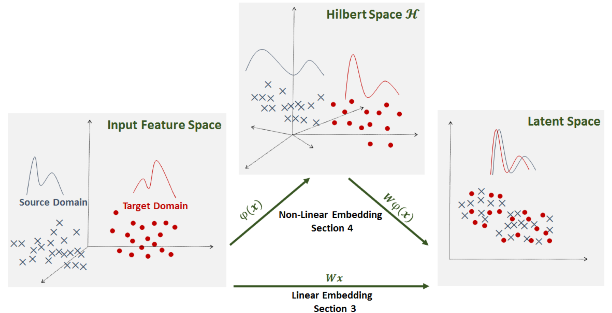
However, marginal distribution alignment assumes that the conditional distribution between two domain are similar to each other once the marginal distribution is aligned. In the real case, such an assumption is usually not valid; therefore, the conditional distribution should also be aligned.

4.2.2 Conditional Distribution Adaptation

In this setting, we assume that the conditional distribution is varied between two domains ($P(\mathcal{Y_{S}}|\mathcal{X_{S}})\neq P(\mathcal{Y_{T}}|\mathcal{X_{T}})$). Many methods minimize the conditional distribution distance between the source and target domain as follows.

$$\min d_{\mathcal{H}\Delta\mathcal{H}}(\mathcal{D_{S}},\mathcal{D_{T}})\approx||P(\mathcal{Y_{S}}|\mathcal{X_{S}})-P(\mathcal{Y_{T}}|\mathcal{X_{T}})||,$$ (3)

Fig. 5 also shows the conditional distribution adaptation, and it focuses on aligning the categorical distributions. However, due to the unlabeled target domain, such an alignment is difficult. Therefore, many methods take advantage of pseudo labels of the target domain.

Figure 8: The scheme of stratied transfer learning (STL) model (image from gong2016domain ).

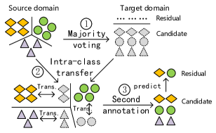
In this scope, Satpal and Sarawagi satpal2007domain proposed conditional probability models via feature subsetting. They combined conditional random fields and conditional probability adaptation to reduce the prediction error. Elsewhere gong2016domain , they proposed to extract conditional transferable components (CTC) from conditional distribution first, and then the marginal distribution is modeled. Later, Wang et al. wang2018stratified introduced the stratified transfer learning (STL) model. Most previous models are based on the global domain shift (inter-class transfer). However, it ignored intra-class transfer. Since the intra-class transfer can utilize the intra-class features, it is able to achieve a better transfer performance. The basic idea of the STL method has three steps. At the first step, majority voting is used to generate pseudo-labels for uncalibrated location behavior; then, as the next step in the reproducing kernel Hilbert space, the intra-class correlation is used to reduce the dimensionality adaptively. Note that dimensionality reduction adaptively makes the correlation between behavior data in different situations. Finally, the accurate calibration of unknown data is realized by secondary calibration. To determine the intra-class transfer, they calculated the MMD for each class using the equation given below:

$$Dist(\mathcal{D}_{S},\mathcal{D}_{T})=\sum_{c=1}^{C}||\frac{1}{n_{c}}\sum_{x_{i}\in\mathcal{D_{S}^{C}}}\phi{(x_{i})}-\frac{1}{m_{C}}\sum_{x_{j}\in\mathcal{D_{T}^{C}}}\phi{(x_{j})}||_{\mathcal{H}}^{2},$$ (4)

where $C$ represents label categories, $\mathcal{D_{S}^{C}}$ and $\mathcal{D_{T}^{C}}$ is the $C$ category of the source and the target domains, respectively. The STL method carried out cross-location behavior recognition experiments using a large number of behavior recognition data.

Although the conditional distribution alignment shows a higher performance than marginal distribution alignment, it still lacks the consideration of overall shape adaptation. Therefore, joint alignment of these two distributions is necessary.

4.2.3 Joint Distribution Adaptation

In this setting, many methods minimize the joint distribution distance between the source domain and the target domain in Eq. (5).

$$\min d_{\mathcal{H}\Delta\mathcal{H}}(\mathcal{D_{S}},\mathcal{D_{T}}) \approx\ ||P(\mathcal{X_{S}})-P(\mathcal{X_{T}})||+$$ (5)

$$||P(\mathcal{Y_{S}}|\mathcal{X_{S}})-P(\mathcal{Y_{T}}|\mathcal{X_{T}})||,$$

The joint distribution adaptation corresponds to the last distribution in Fig. 5. Joint distribution adaptation (JDA) long2013transfer was proposed to reduce the marginal and conditional distributions. The main idea of the JDA method is to find a transformation $A$ to reduce the distance between $P(A^{T}\mathcal{X_{S}})$ and $P(A^{T}\mathcal{X_{T}})$. The distance between $P(\mathcal{Y_{S}}|A^{T}\mathcal{X_{S}})$ and $P(\mathcal{Y_{T}}|A^{T}\mathcal{X_{T}})$ also should be minimized. JDA model can be divided into two steps: marginal distribution adaptation and conditional distribution adaptation. For the marginal distribution adaptation, it aimed to minimize Eq. (6).

$$||\frac{1}{\mathcal{N_{S}}}\sum_{i=1}^{\mathcal{N_{S}}}A^{T}\mathcal{X}_{\mathcal{S}}^{i}-\frac{1}{\mathcal{N_{T}}}\sum_{j=1}^{\mathcal{N_{T}}}A^{T}\mathcal{X}_{\mathcal{T}}^{j}||_{\mathcal{H}}^{2},$$ (6)

For conditional distribution adaptation, it aimed to minimize Eq. (7).

$$\sum_{c=1}^{C}||\frac{1}{n_{c}}\sum_{x_{i}\in\mathcal{D_{S}^{C}}}A^{T}x_{i}-\frac{1}{m_{c}}\sum_{x_{j}\in\mathcal{D_{T}^{C}}}A^{T}x_{j}||_{\mathcal{H}}^{2},$$ (7)

To realize it, the MMD metric and the pseudo label strategy are adopted. The desired transformation matrix can be obtained by solving a trace optimization problem via eigen-decomposition. Further, it is obvious that the accuracy of the estimated pseudo labels affects the performance of JDA. In order to improve the labeling quality, the authors adopt iterative refinement operations. Specifically, in each iteration, JDA is performed, and then a classifier is trained on the instances with the extracted features. Next, the pseudo labels are updated based on the trained classifier. After that, JDA is performed repeatedly with the updated pseudo labels. The iteration ends when convergence occurs.

In follow-up work, additional loss items are added on the basis of JDA, which greatly improves the effect of transfer learning. Adaptation regularization transfer learning (ARTL) long2013adaptation embedded the JDA model into a minimum structure risk framework, which represents the directed learning classifier. The authors also proposed two specific algorithms under this framework based on different loss functions. In these two algorithms, the coefficient matrix for computing MMD and the graph Laplacian matrix for manifold regularization are constructed at first. Then, a kernel function is selected to construct the kernel matrix. Fig. 9 illustrates the scheme of ARTL model.

Figure 9: The scheme of adaptation regularization based transfer learning (ARTL) model. MDA: marginal distribution adaptation; CDA: conditional distribution adaptation; MR: manifold regularization (image from long2013adaptation ).

Visual domain adaptation (VDA) tahmoresnezhad2017visual added the intra-class and inter-class distances in the objective function based on JDA. Hsiao et al., hsiao2016learning controlled the structure invariant based on JDA. Hou et al., proposed a model to select the target domain hou2015unsupervised , and joint geometrical and statistical alignment (JGSA) zhang2017joint calculated intra-class, inter-class distance, and label persistence based JDA. However, a disadvantage of JDA is that marginal distribution and conditional distribution are not equally important. Therefore, balanced distribution adaptation (BDA) wang2017balanced was proposed to solve this problem. The classifier $f$ keeps updating with different steps. It aimed to control the balance between two distributions via the balance factor $\mu$ using Eq. (8).

$$\min d_{\mathcal{H}\Delta\mathcal{H}}(\mathcal{D_{S}},\mathcal{D_{T}})\approx (1-\mu)Dist(P(\mathcal{X_{S}}),P(\mathcal{X_{T}}))$$ (8)

$$+\mu Dist(P(\mathcal{Y_{S}}|\mathcal{X_{S}}),P(\mathcal{Y_{T}}|\mathcal{X_{T}})),$$

where $\mu\in[0,1]$ is the balance factor; $\mu\shortrightarrow 0$ means that there is a significant difference between the source domain and the target domain data and $\mu\shortrightarrow 1$ implies that the source domain and the target domain datasets have high similarity. Wang et al. noted that conditional distribution adaptation is more important. The balance factor can dynamically adjust the importance of each distribution according to the actual data distribution and achieve a good distribution adaptation effect. When $\mu=0$, BDA is the TCA model, and if $\mu=0.5$, the BDA becomes the JDA model. In addition, they also proposed the weighted BDA (WBDA). In WBDA wang2017balanced , the conditional distribution difference is measured by a weighted version of MMD to solve the class imbalance problem.

Figure 10: The scheme of the MEDA model. Features are first learned via manifold kernel $G$. Then, dynamic distribution alignment will learn the domain-invariant classier $f$ (image from wang2018visual ).

Several approaches have addressed the alignment of marginal distribution and conditional distribution of data in special cases. Wang and Mahadevan aligned the source and target domain by preserving the ‘neighborhood structure’ of the data points wang2009manifold . Wang et al. proposed a manifold embedding distribution alignment method (MEDA) (based on work of Gong et al. gong2012geodesic ) to align both the degenerate feature transformation and the unevaluated distributions of both domains wang2018visual . The scheme of MEDA. MEDA model has three fundamental steps: 1) learn features from the manifold based on Gong et al. gong2012geodesic ; 2) use dynamic distribution alignment to estimate the marginal and conditional distributions of data; and, 3) update the classified labels based on estimated parameters.

The classifier ($f$) is defined as:

$$f= \mathop{\arg\min}_{f\in\mathcal{H}_{k}}\sum_{i=1}^{\mathcal{N_{S}}}\mathop{l}(f(g(\mathcal{X}_{\mathcal{S}}^{i})),\mathcal{Y}_{\mathcal{S}}^{i})+\eta||f||_{K}^{2}+$$ (9)

$$\lambda\overline{D_{f}}(\mathcal{D_{S}},\mathcal{D_{T}})+\rho R_{f}(\mathcal{D_{S}},\mathcal{D_{T}})$$

where $\mathcal{H}_{k}$ represents kernel Hilbert space; $l(\cdot,\cdot)$ is the loss function; $g(\cdot)$ is a feature learning function in Grassmannian manifold gong2012geodesic ; $\mathcal{X_{S}}$ is the learned features from one of ImageNet models, $||f||_{K}^{2}$ is the squared norm of $f$; $\overline{D_{f}}(\cdot,\cdot)$ represents the dynamic distribution alignment; $R_{f}(\cdot,\cdot)$ is a Laplacian regularization; $\eta$, $\lambda$, and $\rho$ are regularization parameters. Here, the term $\mathop{\arg\min}_{f\in\mathcal{H}_{k}}\sum_{i=1}^{\mathcal{N_{S}}}\mathop{l}(f(g(\mathcal{X}_{\mathcal{S}}^{i})),\mathcal{Y}_{\mathcal{S}}^{i})+\eta||f||_{K}^{2}$ is the source structure risk minimization (SRM). We can only employ the SRM on $\mathcal{X_{S}}$, since there are few labels (perhaps no labels) for $\mathcal{X_{T}}$. By training the classifier from Eq. (9), we can predict labels of test data. Here, the balance factor $\mu$ minimizes MMD, and it can dynamically change according to the importance between source and target domain. Therefore, it achieves a higher accuracy (MEDA $>$ BDA $>$ JDA $>$ TCA $>$ conditional distribution adaptation $>$ marginal distribution adaptation zhang2019transductive ). Zhang et al. zhangcorrelated2021 proposed to extract both marginal and condiction features from a pre-trained ImageNet model to form the joint features and then minimize the joint distribution between the two domains based on MEDA.

Note that most feature selection and distribution alignment methods focus on the explicit features in the original feature space. In contrast, subspace learning also focuses on some implicit features in an underlying subspace, which can show the geometry of data. Therefore, subspace learning can play various roles in the feature transformation process.

4.3 Subspace learning methods

There are two sub-categories of subspace learning models: feature alignment and manifold learning. Feature alignment methods aim to align the source feature with target features. One of the earliest subspace learning methods is called subspace alignment (SA) fernando2013unsupervised . It can align the source domain and target domain via PCA with a lower subspace dimensionality $d$, which is determined by the minimum Bregman divergence of two subspaces and it minimizes the following function:

$$F(M)=||\mathcal{X}_{\mathcal{S}}^{{}^{\prime}}M-\mathcal{X}_{\mathcal{T}}^{{}^{\prime}}||_{F}^{2},$$ (10)

where $||\cdot||_{F}^{2}$ is the Frobenius norm and $M$ is the transformation matrix, and $\mathcal{X}_{\mathcal{S}}^{{}^{\prime}}\in\mathbb{R}^{\mathcal{N_{S}}\times d}$ and $\mathcal{X}_{\mathcal{T}}^{{}^{\prime}}\in\mathbb{R}^{\mathcal{N_{T}}\times d}$ are generated from the first $d$ eigenvectors from the original domain data ($\mathcal{X}_{\mathcal{S}}^{{}^{\prime}}$ and $\mathcal{X}_{\mathcal{T}}^{{}^{\prime}}$ are the representations of the source and target data in the reduced dimensionality subspace). Then, a learner can be trained on the transformed matrix $F(M)$.

Figure 11: The scheme of SDA model. The model considered the subspace alignment and distribution adaptation (image modified from wang2018visual ).

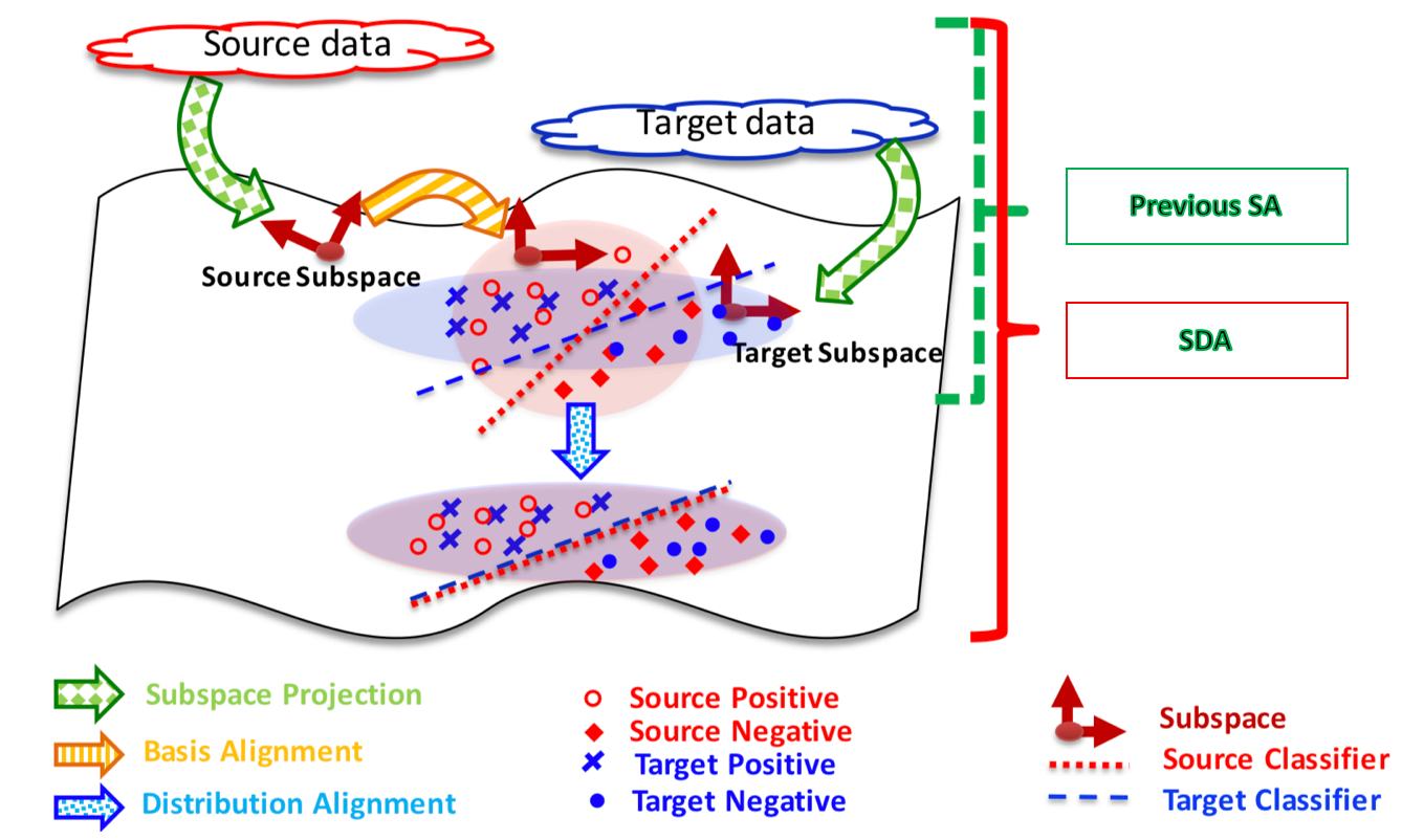
However, SA did not take the difference between the source distribution and the target distribution into account. Sun et al. sun2015subspace proposed the subspace distribution alignment, which can not only align the feature space but also align the distributions of domains. The SDA model improves the domain alignment via the distribution alignment. They first projected the labeled source-domain instances to the source subspace, then mapped to the target subspace, and finally mapped back to the target domain.

One advantage of subspace-based methods is that the calculation is simple and efficient. Similarly, the linear correlation alignment (CORAL) minimized domain shift by aligning the second-order statistics of source and target distributions sun2016return ; it solved the following optimization problem:

$$\min_{A}||C_{\hat{S}}-C_{T}||_{F}^{2}=\min_{A}||A^{T}C_{S}A-C_{T}||_{F}^{2},$$ (11)

where $A$ is the transformation matrix, $C_{\hat{S}}$ is the covariance of the transformed source features $X_{S}A$. $C_{S}$, and $C_{T}$ are covariance matrices of source and the target domain, respectively. The main process of CORAL is updating the source data using its covariance followed by the “re-coloring” of the target covariance matrix.

There are also approaches to minimize domain discrepancy based on the spectral feature alignment using graph theory. Pan et al. proposed a spectral feature alignment (SFA) pan2010cross method. It can identify the domain-specific and domain-independent features in different domains and then aligns these domain-specific features by constructing a lower-dimensional feature representation.

Figure 12: The scheme of sampling geodesic flow (SGF) method (image from gopalan2011domain ).

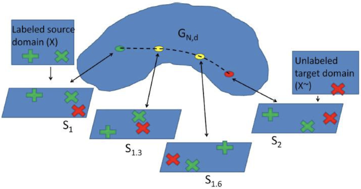
Manifold learning models aim to map the data on Riemannian manifold and reduce the distance of the two domains on the manifold. One of the earliest manifold learning methods is based on the Grassmannian manifold, which learns the intermediate features between the sub-source and the sub-target domain via a Grassmannian manifold. Gopalan et al. gopalan2011domain proposed a sampling geodesic flow (SGF) method to learn the intermediate features between the sub-source and the sub-target domain via the geodesic (shortest path) on Grassmannian manifold. To obtain the samples between $\mathcal{X_{S}}$ and $\mathcal{X_{T}}$, sampling geodesic flow (SGF) consists of the following steps: 1) calculate the geodesic which starts from the source and ends with target domains on the Grassmannian in the subspace; 2) sample a given number of subspaces along the geodesic; 3) project the original feature vectors into samples’ subspaces and utilize the results as new features; 4) reduce the dimensionality of the new features; and, 5) use the resulting new (reduced) feature vectors to train the classifiers and evaluate on target data.

However, SGF has several limitations. Gong et al. have noted that it is difficult to choose an optimal sampling strategy gong2012geodesic . Also, several basic parameters need to be adjusted: the sample size, the reduced dimension of the subspace, and how to represent original data using new samples. Moreover, SGF has high time complexity, making sampling slow when many points are needed.

Figure 13: The scheme of geodesic flow kernel (GFK) model. It considers all samples points on the geodesic (image from gong2012geodesic ).

To overcome the limitations of unknown sampling size and subspace dimensionality, the geodesic flow kernel (GFK) was proposed by Gong et al. gong2012geodesic . They integrated all samples along the “geodesic” (the shortest distance between two points on the manifold), which is shown in the following equation.

$$\int_{0}^{1}(\Phi(t)^{T}x_{i})^{T}(\Phi(t)^{T}x_{i})dt=x_{i}^{T}Gx_{i},$$ (12)

where $\Phi$ is the projection matrix. The GFK model contained the following steps: 1) compute the optimal reduced dimensionality of the subspaces; 2) calculate the geodesic curve; 3) compute the geodesic flow kernel; and, 4) use the kernel to train a classifier with labeled data and test on unlabeled data. However, dimensionality is a hyper-parameter of the GFK model; one needs to calculate the optimal dimensionality. In addition, it has the constraint that the size of dimensionality should be less than half of the minimum dimension of source and test data, which is $d<\frac{1}{2}\min(length(\mathcal{X}_{\mathcal{S}}^{{}^{\prime}}),length(\mathcal{X}_{\mathcal{T}}^{{}^{\prime}}))$, where $length$ refers to the number of features in the sub-source $\mathcal{X}_{\mathcal{S}}^{{}^{\prime}}$ and sub-target $\mathcal{X}_{\mathcal{T}}^{{}^{\prime}}$ domains. In addition, the GFK model will only work well if the dimensionality of each point is far larger than the number of total points.

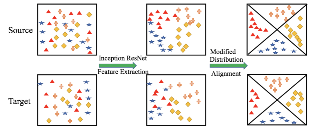
However, none of these models explored the quality of the learned features, i.e., the geodesic path has not been verified. Zhang et al., zhang2019modified found that the SGF method did not provide a correct way to sample the points along the geodesic. We also demonstrated that the “geodesic” from the SGF model is not the true geodesic. They then extracted features from a pre-trained InceptionResNetv2 deep network. The deep features contained detailed information of the object, and the SGF-based manifold learning will destroy this information. They also modified MEDA to form the modified distribution alignment (MDA) model, which improves the performance of the DA problem. The scheme of the MDA model is shown in Fig. 14. Later, They proposed a geodesic sampling on Riemannian manifolds (GSM) zhang2019transductive model to sample intermediate features along the correct geodesic. In the follow-up work, they proposed a subspace sampling demon (SSD) zhang2020domain approach to show the detailed shape deformations and utilize quantitative methods to evaluate learned features. They also proposed a deep spherical manifold Gaussian kernel zhang2021deep2 framework to map the source and target subspaces into a spherical manifold and reduce the discrepancy between them by embedding both extracted features and a Gaussian kernel.

Figure 14: The scheme of MDA model. Features are extracted from the last fully connected layer in InceptionResNetv2 model, and then align the distribution of learned features (image from zhang2019modified ).

(a) SGF gopalan2011domain

(b) GSM zhang2019transductive

(c) SSD zhang2020domain

Figure 15: The comparison of sampling results between the two images (square and circle) with $t=0,\ 0.05,\ 0.5,\ 0.95,\ 1$.

5 Deep Learning Methods

With the popularity of deep learning methods, deep neural networks have shown improved performance in transfer learning. Compared with traditional methods, deep transfer learning directly improves the learning effect on different tasks. Moreover, since deep learning directly learns from raw data, it has two advantages over traditional methods: automatically extracting more expressive features and meeting the end-to-end requirements in practical applications.

Deep learning methods can be classified into homogeneous DA and heterogeneous DA. We focus on deep homogeneous DA. There are six categories of homogeneous deep UDA methods: discrepancy-based, adversarial-based, pseudo-labeling-based, reconstruction-based, representation-based and attention-based methods as shown in Fig 2.

1. Discrepancy-based: these methods minimize the distance between the source domain and the target domain using different statically defined distance functions.

2. Adversarial-based: these methods identify the domain invariant features via two competing networks.

3. Pseudo-labeling-based: these methods generate pseudo labels for the target domain to reduce the domain divergence.

4. Reconstruction-based: these methods map two domains into a shared domain while preserving domain specific features.

5. Representation-based: these methods utilize the trained network to extract intermediate representations as an input for a new network.

6. Attention-based: these methods pay attention to regions of interests (ROIs), which maintains shared information of both source domain and the target domain.

5.1 Discrepancy-based methods

Discrepancy based methods are one of the most popular deep network models, and it aims to decrease the differences between the two domains and align data distributions. Different distance loss functions are usually added in the activation layers of networks. Discrepancy based methods can be further divided into eight subgroups as shown in Fig. 2. We review these different distance functions in the following subsections.

5.1.1 Maximum Mean Discrepancy (MMD)

Maximum Mean Discrepancy (MMD) is one of the most popular distances in minimizing a distance between two distributions, as shown in Eq. (2). It measures the distributions as the squared distance between their embeddings in the reproducing kernel Hilbert space. MMD is also the equivalent to finding the RKHS mapping function, which maximizes the difference in expectations between the two probability distributions in the following equation.

$$MMD(\mathcal{D_{S}},\mathcal{D_{T}})=sup_{f\in\mathcal{H}}||E_{\mathcal{X_{S}}}[f(\mathcal{X_{S}})]-E_{\mathcal{X_{T}}}[f(\mathcal{X_{T}})]||_{\mathcal{H}}^{2},$$ (13)

where $E$ is the distribution expectation, and $f$ is a function or classifier in the deep neural networks.

Based on MMD, Tzeng et al. tzeng2014deep proposed a deep domain confusion (DDC) model; it minimized the following loss function:

$$\mathcal{L}=\mathcal{L}_{C}(\mathcal{X_{S}},\mathcal{Y_{S}})+\lambda MMD^{2}(\mathcal{X_{S}},\mathcal{X_{T}}),$$ (14)

where $\mathcal{L}_{C}(\mathcal{X_{S}},\mathcal{Y_{S}})$ denotes the cross-entropy loss on the available labeled data ($\mathcal{X_{S}}$), and the ground truth labels ($\mathcal{Y_{S}}$), and $MMD^{2}(\mathcal{X_{S}},\mathcal{X_{T}})$ denotes the distance between $\mathcal{X_{S}}$ and $\mathcal{X_{T}}$. The hyperparameter $\lambda$ determines robustness to confuse the domains. DDC model fixed the first seven layers and added the adaptation metric (MMD) in the eighth layer. Later, they extended the DDC model by introducing soft label distribution matching loss tzeng2015simultaneous .

Figure 16: The scheme of the deep domain confusion (DDC) model (image from tzeng2014deep ).

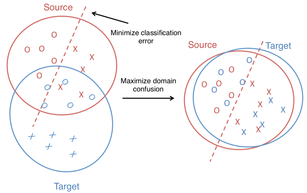
Different from DDC, which used a single layer and linear MMD, the deep adaptation network (DAN) long2015learning model considered several MMDs between several layers and explored multiple kernels for adaptation of the deep representations.

Figure 17: The architecture of deep adaptation network (DAN) model. The features are extracted from frozen (conv1–conv3) and fine-tuning (conv4–conv5) layers. MK-MMD is adapted in fc6–fc8 layers (image from long2015learning ).

Joint adaptation networks (JAN) long2017deep further considered the joint distribution discrepancies (by using joint MMD (JMMD) criteria) of extracted features. In addition, residual transfer networks (RTN) long2016unsupervised added a gated residual layer and relaxed the DAN classifier criteria. Yan et al. yan2017mind proposed a weighted MMD (WMMD) to construct the source distribution using the target domain to reduce the effect of class weight bias. Recently, the multi-representation adaptation network (MRAN) zhu2019multi extended MMD to conditional MMD (CMMD) to reduce the differences between domains. Kang et al. kang2019contrastive extended MMD to the contrastive domain discrepancy loss. It can jointly optimize the intra-class distance and inter-class distance for improving the adaptation performance. Deng et al. deng2020rethinking considered triplet loss to align data distributions from domain-level and class-level. For aligning domain level, they utilized the JMMD metric to reduce the domain-level discrepancy, and similarity guided constraint (SGC) to reduce the class-level discrepancy.

5.1.2 Correlation Alignment (CORAL)

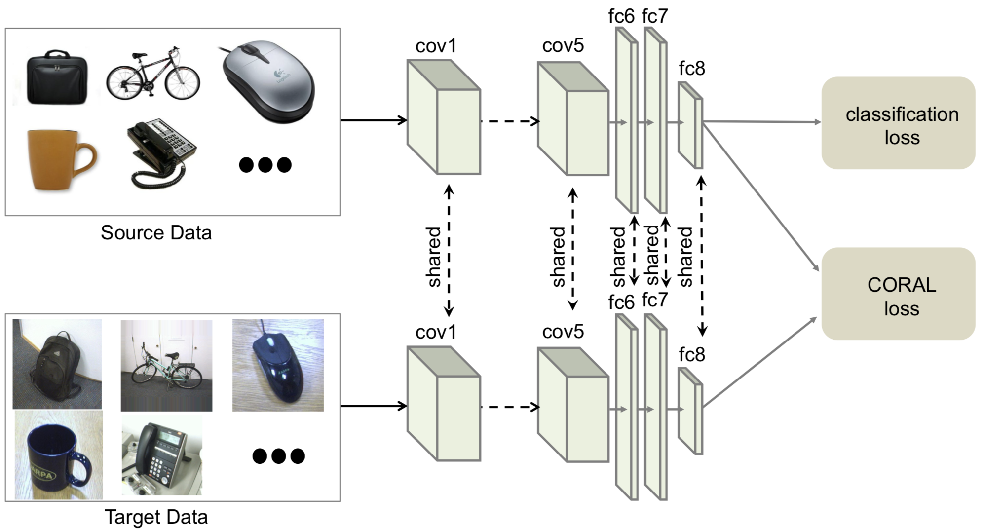
CORAL sun2016deep aims to align the second-order statistics (covariances) between the cross-domain distributions. The Deep CORAL model extended the CORAL model into a deep architecture, and the loss function is defined in Eq. (15).

$$\mathcal{L}_{CORAL}=\frac{1}{4d^{2}}||C_{\mathcal{S}}-C_{\mathcal{T}}||_{F}^{2},$$ (15)

where $d$ is the feature dimensionality, $C_{\mathcal{S}}$ and $C_{\mathcal{T}}$ are the covariance matrices of the source data and the target data, and $||\cdot||_{F}^{2}$ denotes the squared matrix Frobenius norm. Mapped Correlation Alignment (MCA) zhang2018unsupervised projected covariances of different domains from Riemannian manifold to RKHS. It can learn a non-linear mapping via combining MCA loss and classification loss. Chen et al. chen2019joint introduced joint discriminative domain alignment (JDDA), which utilized CORAL loss, and applied a discriminative loss to form an instance-based and center-based discriminative learning scheme for DA. Rahman et al. proposed a model based on the alignment of second-order statistics (covariances) as well as maximized the mean discrepancy of the source and target data rahman2020minimum .

Figure 18: The architecture of Deep CORAL model. It is based on a CNN with a classifier layer, which adds the CORAL loss on the fc8 layer of AlexNet (image from sun2016deep ).

5.1.3 Kullback–Leibler Divergence (KL)

Kullback–Leibler divergence (KL) van2014renyi aims to measure the distance between two distributions ($P(x)$ and $Q(x)$) as follows.

$$D_{KL}(P||Q)=\sum_{x\in\mathcal{X}}P(x)\text{log}\frac{P(x)}{Q(x)},$$ (16)

where $\mathcal{X}$ is the probability space, and KL divergence is an asymmetric distance: $D_{KL}(P||Q)\neq D_{KL}(Q||P)$. Zhuang et al. zhuang2017supervised proposed an approach termed transfer learning with deep autoencoders (TLDA), which adopted two autoencoders for the source and the target domains via minimizing the KL divergence. Meng et al. meng2018adversarial also minimized the Kullback-Leibler divergence between the output distributions of the teacher and student models simultaneously to better align two domains.

5.1.4 Jensen–Shannon Divergence

Jensen–Shannon divergence (JSD) fuglede2004jensen is derived from KL divergence, and it is a symmetric distance.

$$JSD_{KL}(P||Q)=\frac{1}{2}D_{KL}(P||M)+\frac{1}{2}D_{KL}(Q||M),$$ (17)

where $M=\frac{1}{2}(P+Q)$.

Jiang et al. jiang2020resource proposed resource efficient domain adaptation (REDA) to distill transfer features across domain by minimizing the JSD between the probability predictions of the major classifier and the shallower classifiers.

Figure 19: The architecture of Sliced Wasserstein discrepancy (SWD) model (image from lee2019sliced ).

5.1.5 Wasserstein Distance

The Wasserstein metric vallender1974calculation is another discrepancy metric to measure the distance among the different domain samples. This distance is defined in a metric space ($M,\rho$), and $\rho(x_{1},x_{2})$ is the distance between two samples as shown in the following equation.

$$W(P(\mathcal{X_{S}}),P(\mathcal{X_{T}})) =\{\inf_{\mu\in\Gamma(P(\mathcal{X_{S}}),P(\mathcal{X_{T}}))}$$ (18)

$$\int\rho(x_{1},x_{2})^{p}d\mu(x_{1},x_{2})\}^{1/p}$$

Damodaran et al. bhushan2018deepjdot jointly matched feature and label space distributions based on Wasserstein distance, and they not only learned the new data representations aligned between the source and target domain, but also simultaneously preserved the discriminative information. Sliced Wasserstein discrepancy (SWD) lee2019sliced utilized the geometrical 1-Wasserstein distance as the discrepancy measure for obtaining the dissimilarity probability of source and target domains.

5.1.6 Mutual Information

Mutual Information (MI) kraskov2004estimating aims to find the similarity between two distributions in Eq. (19).

$$MI(P(\mathcal{X_{S}}),P(\mathcal{X_{T}}))=\sum_{x_{1}\in\mathcal{X_{S}}} \sum_{x_{2}\in\mathcal{X_{T}}}P(\mathcal{X_{S}},\mathcal{X_{T}})$$ (19)

$$\text{log}\frac{P(\mathcal{X_{S}},\mathcal{X_{T}})}{P(\mathcal{X_{S}})P(\mathcal{X_{T}})},$$

Gholami et al. gholami2020unsupervised employed a deep learning model to jointly maximize the mutual information between the domain labels and private (domain-specific) features while minimizing the mutual information between the domain labels and the shared (domain-invariant) features. Xie et al. xie2020mi disentangled the content features from domain information for both the source and translated images and then maximized the mutual information between the disentangled content features to preserve the image-objects using a discriminator.

5.1.7 Entropy Minimization

Entropy minimization grandvalet2005semi aims to find the minimal entropy between distributions of two samples. Feature transfer network (FTN) sohn2018unsupervised first separated the transformed source domain and target domain using an entropy minimization loss function to enhance the discriminative ability of FTNs in the target domain. Later, Roy et al. roy2019unsupervised proposed min-entropy consensus (MEC) method to jointly merge consistency loss and entropy loss to improve the domain adaptation as shown in Eq. (LABEL:eq:em).

$$L^{t}(B_{1}^{t},B_{2}^{t})=\frac{1}{m}\sum_{i=1}^{m}l^{t}(x_{i}^{t_{1}},x_{i}^{t_{2}}),$$ (20)

where $$l^{t}(x_{i}^{t_{1}},x_{i}^{t_{2}})=-\frac{1}{2}\max_{y\in Y}(\log p(y|x_{i}^{t_{1}})+\log p(y|x_{i}^{t_{2}}))$$

where $x_{i}^{t_{1}}\in B_{1}^{t}$ and $x_{i}^{t_{2}}\in B_{2}^{t}$, and $B_{1}^{t},B_{2}^{t}$ are two different target batches.

Mancini et al. mancini2018boosting further incorporated MEC loss with the multiple domain predictions on perturbations to achieve the consistency and reduce entropy for the perturbed domain predictions of the same input features.

Figure 20: The architecture of min-entropy consensus (MEC) (image from roy2019unsupervised ).

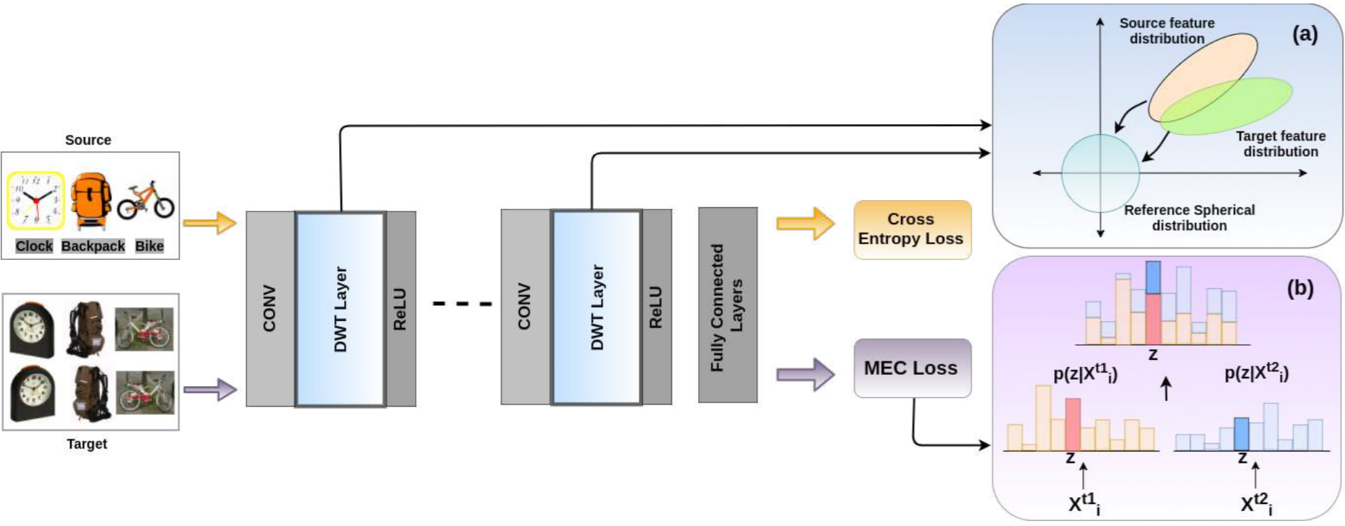
5.1.8 Batch Normalization

Batch Normalization (BN) ioffe2015batch has been widely used in deep networks to decrease the covariance shift.

In multi-source DA mancini2018boosting , Mancini et al. extended batch normalization of DA layer to a new batch normalization layer (mDA-layer). This mDA-layer can re-normalize the multi-modal feature distributions as shown in the following equation.

$$mDA(x_{i},w_{i},\hat{\mu},\hat{\sigma})=\sum_{d\in D}w_{i,d}\frac{x_{i}-\hat{\mu}_{d}}{\sqrt{\hat{\sigma}_{d}^{2}+\epsilon}},$$ (21)

where $w_{i}=[w_{i,d}]_{d\in D}$, $\hat{\mu}=[\hat{\mu}_{d}]_{d\in D}$ and $\hat{\sigma}=[\hat{\sigma}_{d}^{2}]_{d\in D}$.

Li et al. li2018adaptive introduced an adaptive batch normalization (AdaBN) model to improve the generalization ability of the deep neural network. AdaBN can change the data of BN layers of the target domain via data of the source domain and also update the weights in CNN for DA. Change et al. chang2019domain proposed domain specific batch normalization (DSBN) based on multiple sets of BN layers. The DSBN can estimate the mean and variance of multiple domains, and it can capture the domain-specific features, and then the domain-invariant features can be better extracted from deep neural networks.

Figure 21: The architecture of domain specific batch normalization (DSBN) (image from chang2019domain ).

5.1.9 Least Squares

Least Squares zhang2021deep33 aims to approach data distribution via estimating the slope and intercept in the latent space. Deep least squares alignment (DLSA) zhang2021deep33 first propose to minimize the slop and intercept differences to realize domain divergence reduction with least squares estimation. They first minimized the marginal distribution as follows.

$$\mathcal{L_{M}}=||\hat{a}_{\mathcal{S}}-\hat{a}_{\mathcal{T}}||_{F}^{2}+\gamma||\hat{b}_{\mathcal{S}}-\hat{b}_{\mathcal{T}}||_{F}^{2},$$ (22)

where $\mathcal{M}$ denotes marginal distribution, $||\cdot||_{F}$ is the Frobenius norm, and $\gamma$ balances the scale between two terms. The first term enforces small differences of slope between two domains, while the second enforces small differences of intercept between two domains. They also minimized conditional distribution via reducing the categorical slop and intercept differences.

Figure 22: The architecture of deep least squares alignment (DLSA) (image from zhang2021deep33 ).

5.2 Adversarial-based methods

Recently, adversarial-based methods have become an increasingly popular method to reduce domain discrepancy between different domains by using an adversarial objective. With the advent of generative adversarial networks (GAN) goodfellow2014generative , adversarial learning models have been found to be an impactful mechanism for identifying invariant representations in domain adaptation. Adversarial learning also contains a feature extractor and a domain discriminator. The domain discriminator aims to distinguish the source domain from the target domain, while the feature extractor aims to learn domain-invariant representations to fool the domain discriminator tzeng2017adversarial ; long2018conditional ; zhang2019domain ; liu2019transferable ; wei2021metaalign ; ma2021adversarial ; jing2021adversarial ; akkaya2021self ; zhang2021adversarial2 ; zhang2021adversarial_re . The target domain error is expected to be minimized via minimax optimization.

Figure 23: The architecture of domain adversarial neural networks (DANN) model. It includes a feature extractor (green), a label predictor (blue), and a domain classifier (pink) (image from ganin2016domain ).

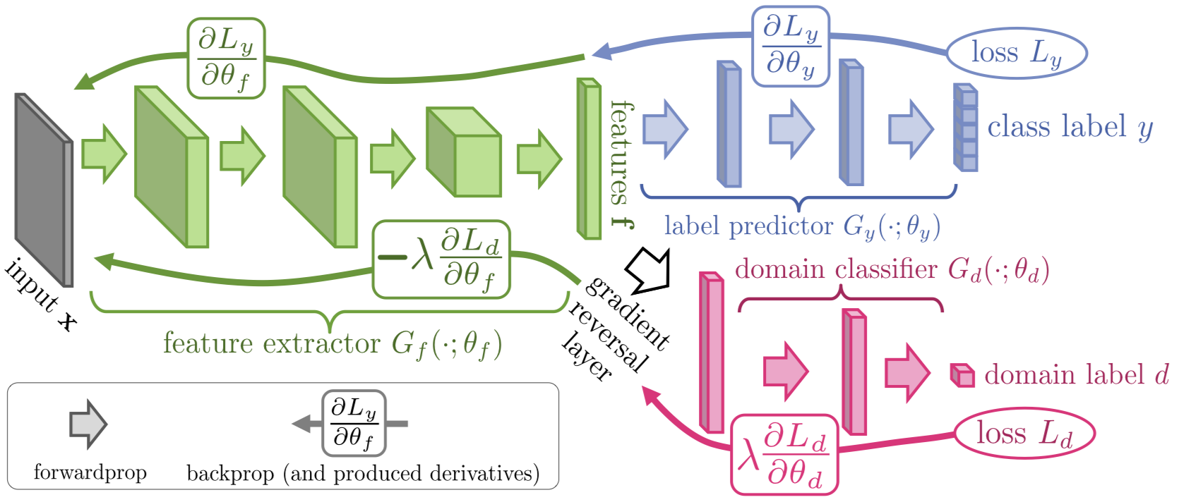
The domain adversarial neural network (DANN) ganin2016domain is one of the first adversarial methods for adversarial based DA. DANN considered a minimax loss to integrate a gradient reversal layer to promote the discrimination of source and target domains ganin2016domain . Unsupervised DA is achieved by the gradient reversal layer that multiplies the gradient by a certain negative constant during the backpropagation-based training to ensure that the feature distributions over the two domains are made indistinguishable. The domain discriminator typically minimizes the binary cross-entropy loss as follows.

Figure 24: The architecture of adversarial discriminative domain adaptation (ADDA) model. The dash lines represents fixed network parameters (image from tzeng2017adversarial ).

The adversarial discriminative domain adaptation (ADDA) uses an inverted label GAN loss to split the source and target domains, and features can be learned separately tzeng2017adversarial . The coupled generative adversarial networks liu2016coupled consisted of a series of GANs, and each of them can represent one of the domains. Cao et al. cao2018partial proposed a partial transfer learning model. They noted that in the era of big data, we usually have a lot of source domain data. These source domain data are usually richer in categories than target domain data. For example, the image classifier based on ImageNet training must categorize thousands of categories. When we use it in practice, the target domain is often only a part of the categories. This leads to a problem: categories that exist only in the source domain will have a negative impact on label migration results. The collaborative adversarial network (CAN) zhang2018collaborative added several domain classifiers on multiple CNN feature extraction blocks on each domain classifier for DA. Chen et al. chen2019joint proposed joint domain alignment and discriminative feature learning. It benefits both domain alignment and final classification. Two discriminative feature learning methods are proposed (instance-based and center-based), which can guarantee the domain invariant features.

The joint adaptation network (JAN) long2017deep combined MMD with adversarial learning to align the joint distribution of multiple domain-specific layers across domains. Enhanced transport distance (ETD) measured domain discrepancy by establishing the transport distance of attention perception as the predictive feedback of iterative learning classifiers li2020enhanced . Cycle-consistent adversarial domain adaptation (CyCADA) proposed cycle-consistency loss to enforce local and global structural consistency between two domains hoffman2018cycada . To improve results, many methods utilize image-level adaptation (to maintain the consistency of images during training) to help feature alignment. Progressive domain adaptation hsu2020progressive combined feature alignment with image-level adaptation. They first adopted a model between source and intermediate domain via image translation. The transformed images have the same label mapped from the source domain and are treated as simulated training images for the target domain. Then, the intermediate and target domains are aligned. Zhang et al. zhang2018collaborative reweighted the target samples, which can confuse the domain discriminator. The domain-symmetric network (SymNet) is a symmetrically designed source and target classifier based on an additional classifier. The proposed category-level loss can improve the domain-level loss by learning the invariant features between two domains zhang2019domain .

Miyato et al. miyato2018virtual incorporated virtual adversarial training (VAT) in semi-supervised contexts to smooth the output distributions as a regularization of deep networks. Later, virtual adversarial domain adaptation (VADA) improved adversarial feature adaptation using VAT. It generated adversarial examples against only the source classifier and adapted on the target domain shu2018dirt . Unlike VADA method, transferable adversarial training (TAT) adversarially generated transferable examples that fit the gap between source and target domain liu2019transferable . Xu et al. xu2019adversarial constructed a GAN-based architecture named adversarial domain adaptation with domain mixup (DM-ADA). It maps the two domains to a common potential distribution, and effectively transfers domain knowledge. Zhang et al. zhang2020hybrid introduced a hybrid adversarial network (HAN) to minimize the source classifier loss, conditional adversarial loss, and correlation alignment loss. A new adaptation layer was used to further improve the performance in the HAN model.

5.3 Pseudo-labeling-based methods

Pseudo-labeling is another technique to address UDA and also achieves substantial performance on multiple tasks. Pseudo-labeling typically generates pseudo labels for the target domain based on the predicted class probability saito2017asymmetric ; xie2018learning ; zhang2018collaborative ; chen2019progressive ; zhang2020adversarial3 . Under such a regime, some target domain label information can be considered during training. In deep networks, the source classifier is usually treated as an initial pseudo labeler to generate the pseudo labels (and use them as if they were real labels). Different algorithms are proposed to obtain additional pseudo labels and promote distribution alignment between the two domains.

Figure 25: The architecture of progressive feature alignment network (PFAN) (image from chen2019progressive ).

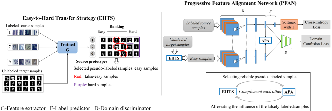
An asymmetric tri-training method for UDA has been proposed by Saito et al. to generate pseudo labels for target samples using two networks, and the third can learn from them to obtain target discriminative representations saito2017asymmetric . Xie et al. xie2018learning proposed a moving semantic transfer network (MSTN) to develop semantic matching and domain adversary losses to obtain pseudo labels. Zhang et al. zhang2018collaborative designed a new criterion to select pseudo-labeled target samples and developed an iterative approach called incremental collaborative and adversarial network (iCAN), in which they select samples iteratively and retrain the network using the expanded training set. Progressive feature alignment network (PFAN) chen2019progressive aligns the discriminative features across domains progressively and employs an easy-to-hard transfer strategy for iterative learning. Chang et al. chang2019domain proposed to combine the external UDA algorithm and the proposed domain-specific batch normalization to estimate the pseudo labels of samples in the target domain and more effectively learn the domain-specific features. Constrictive adaptation network (CAN) also employed batch normalization layers to capture the domain-specific distributions kang2019contrastive . Zhang et al. zhang2020label offers a label propagation with augmented anchors (A2LP) method to improve label propagation via generation of unlabeled virtual samples with high confidence label prediction. Adversarial continuous learning in UDA (ACDA) zhang2020adversarial3 increased robustness by incorporating high-confidence samples from the target domain to the source domain. They further proposed a pre-trained features selection and recurrent pseudo-labeling (PRPL) zhang2021efficient model to continuously generate high-quality pseudo labels.

Figure 26: The architecture of domain separation networks (DSN) model. It consists of four loss functions: $l_{class}$, $l_{recon}$, $l_{difference}$ and $l_{similarity}$ (image from bousmalis2016domain ).

5.4 Reconstruction-based methods

Reconstruction based methods aim to reconstruct all domain samples to make better representations of domains, while preserving domain specific features.

Encoder-decoder style is one representative reconstruction based method. It first encodes input images to some hidden features by the encoder, then decodes these features back for reconstructed images by the decoder. The domain-invariant features are learned by a shared encoder while domain-specific features are preserved by reconstruction loss ghifary2016deep . Stacked denoising autoencoders (SDA) vincent2008extracting is one of the first deep models for domain adaptation and aimed to find the common features between source and target domains via denoising autoencoders. The objective function is defined in Eq. 24.

$$\theta^{\star}\theta^{{}^{\prime}\star} =\arg\min_{\theta^{\star}\theta^{{}^{\prime}\star}}\frac{1}{n}\sum_{i=1}^{n}L(x^{(i)},z^{(i)})$$ (24)

$$=\arg\min_{\theta^{\star}\theta^{{}^{\prime}\star}}\frac{1}{n}\sum_{i=1}^{n}L(x^{(i)},g_{\theta^{\prime}}(f_{\theta}(x^{(i)}))),$$

where $x$ is the input vector, $L$ is the loss function, which is squared error: $L(x,z)=||x-z||^{2}$, $\theta$ is the parameter in the autoencoders, and $f$ and $g$ are mapping functions.

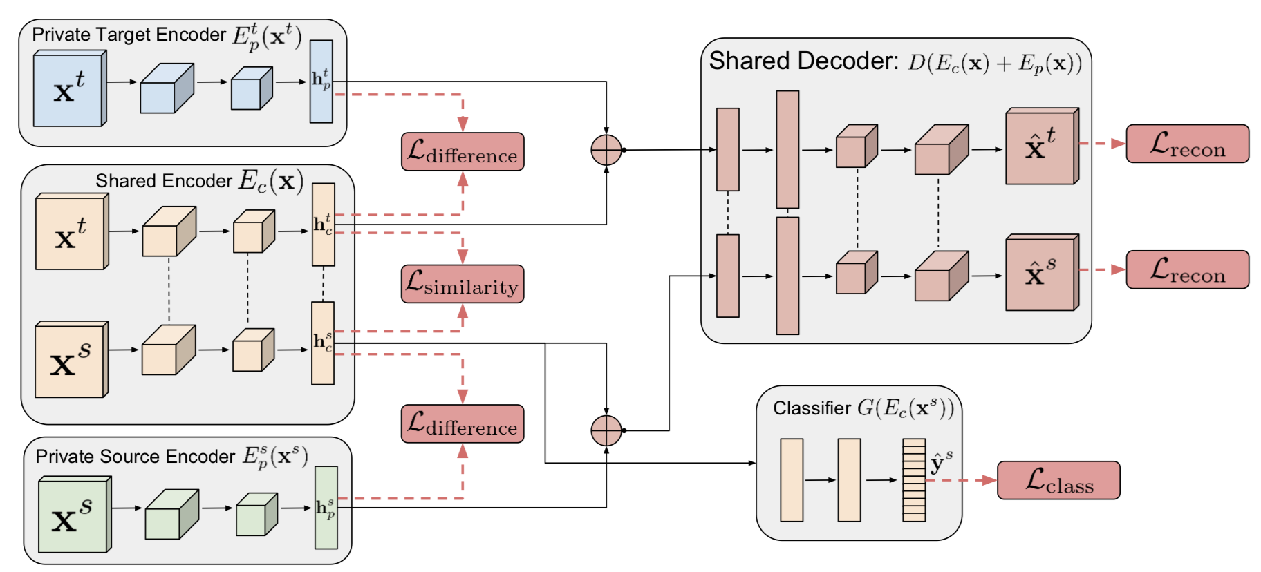
To reduce the computational costs of SDA model, Chen et al. chen2012marginalized introduced a marginalized SDA (mSDA) model to denoise the marginal noise with a closed-form solution without using a stochastic gradient descent strategy. Multi-task autoencoder (MTAE) ghifary2015domain learned intra- and inter-domain reconstruction to represent domain invariances. Ghifary et al. ghifary2016deep proposed a deep reconstruction classification network (DRCN) to learn a shared encoding representation, which aims to minimize domain discrepancy. Zhang et al. zhuang2015supervised proposed transfer learning with deep auto-encoders using Kullback–Leibler divergence to reduce the discrepancy between the source and target distributions. Domain separation networks (DSN) bousmalis2016domain introduced the notion of a private subspace for each domain, which captures domain-specific properties, such as background and low-level image statistics. The shared subspace is enforced through the use of autoencoders and explicit loss functions, which can capture common features between the two domains. The loss function is defined as following:

$$l=l_{t}ask+\alpha l_{recon}+\beta l_{difference}+\gamma l_{similarity},$$ (25)

where $l_{task}$ is the loss of the training, $l_{recon}$ is the loss of the reconstruction, $l_{difference}$ is the difference between public and private space, and $l_{similarity}$ is the similarity of public space of source and target domain. The architecture of DSN is shown in Fig.26.

5.5 Representation-based methods

Representation based methods utilize the trained network to extract intermediate representations as an input for a new network.

Figure 27: The architecture of cross domain representation disentangler (CDRD) model (image from liu2018detach ).

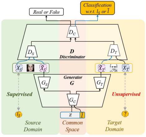
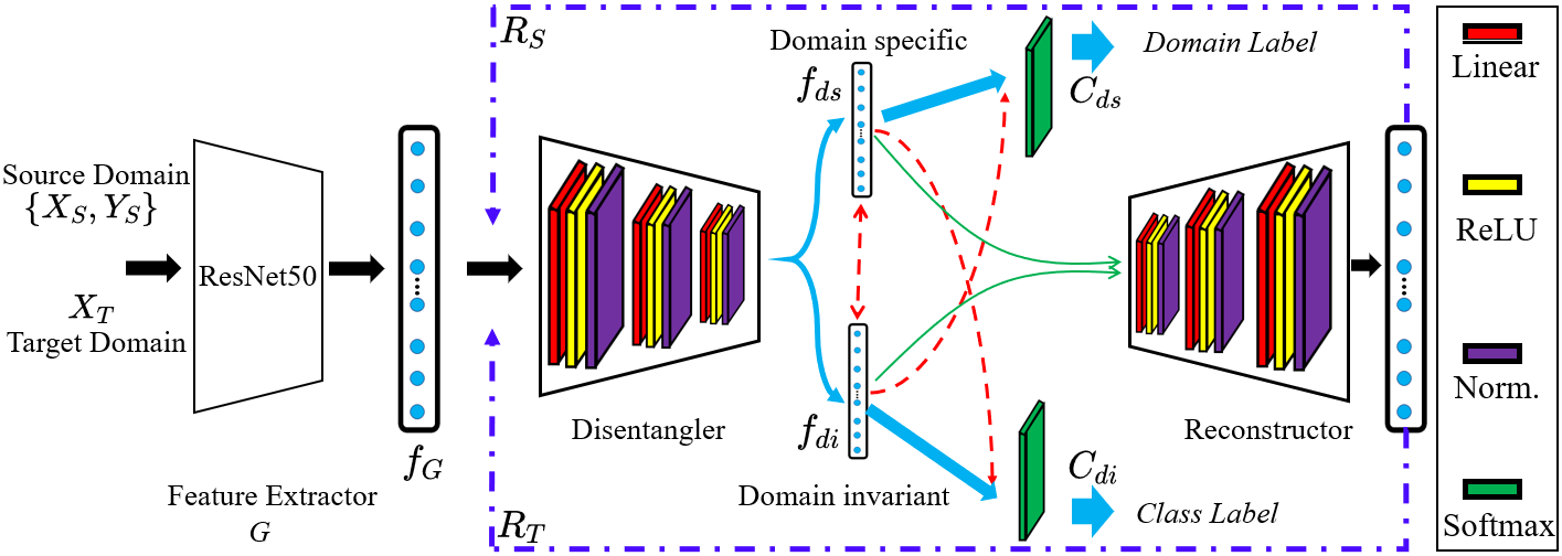
One common method is called disentanglement representation, which is based on class labels to gain invariant feature representation. Cross domain representation disentangler (CDRD) liu2018detach bridged the labeled source domain and unlabeled target domain by jointly learning cross-domain feature representation disentanglement and adaptation. The common space is optimized with both the labeled source domain and the unlabeled target domain. Hence, the shared weighted common space can bridge the gap between high and coarse-level representations of cross-domain data. Gonzalez et al. gonzalez2018image proposed an image-to-image translation for representation disentangling based on GANs and cross-domain autoencoders. They separated the internal representation into three parts: a shared part, which contains the domain-invariant features for two domains; and two exclusive parts, which contain the domain-specific features. Their model can be applied to multiple tasks, such as diverse sample generation, cross-domain retrieval, domain-specific image transfer, and interpolation. Liu et al. liu2018unified introduced a unified feature disentanglement network (UFDN) to learn domain-invariant representation from multiple domains for image translation and manipulation. Peng et al. peng2019domain minimized mutual information between domain-specific and domain-invariant features to pursue implicit domain-invariant features, which can improve the performance of the target domain. Gholami et al. gholami2020unsupervised presented a multi-target domain adaptation information-theoretic approach (MTDA-ITA) to find a shared latent space of all domains by simultaneously identifying the remaining private domain-specific factors. They utilized a unified information-theoretic approach to disentangle the shared and private information while establishing a connection between latent representations and the observed data. Their model can adapt from a single source to multiple target domains. However, these disentanglement-based methods are still difficult to guarantee the full separation between domain-specific features and domain invariant features. Also, the reconstruction of these two features is less considered. Zhang et al. zhang2021enhanced propose an enhanced separable disentanglement (ESD) model. It can teach a disentangler to distill domain-specific and domain-invariant features from the two domains. They then applied feature separation maximization processes to enhance the disentangler to remove contamination between these two features. A reconstructor is used to recover original feature prototypes to further improve the performance of the model.

Figure 28: The architecture of enhanced separable disentanglement (ESD) model (image from zhang2021enhanced ).

5.6 Attention-based methods

Attention based methods pay attention to region of interests (ROIs) from the source domain to the target domain, which can make the deep neural networks focus on some spatial parts of both domains.

Wang et al. wang2017residual proposed a residual attention network (RAN), which added an attention mechanism in a convolutional neural network. RAN can generate attention-aware features via stacking attention modules. The attention module contains three key parameters: the number of pre-processing Residual Units before splitting into the trunk branch and mask branch, the number of Residual units in the trunk branch, and the number of Residual units between the adjacent pooling layer in the mask branch. However, RAN has the issue of negative local attention in transferring tasks. Later, the transferable attention for domain adaptation (TADA) model reduced the effects of negative transfer. It applied transferable global attention based on local attention. There are two types of complementary transferable attention: local attention can generate transferable regions by multiple region-level domain discriminators, and global attention can generate transferable images by image-level domain discriminator.

Figure 29: The architecture of residual attention network (RAN) (image from wang2017residual ).

Zhuo et al. zhuo2017deep presented a deep unsupervised convolutional domain adaptation (DUCDA) model, which consists of source classification loss and correlation alignment (CORAL) loss. The CORAL loss measured the discrepancy between attention maps for both source and target domains, and it was used on both convolutional layers and fully connected layers. Moon et al. moon2017completely proposed completely heterogeneous transfer learning (CHTL) to filter and suppress irrelevant source samples using an attention mechanism and designed an unsupervised transfer loss to learn the knowledge between two domains. Kang et al. kang2018deep presented a deep adversarial attention alignment model, which transfers knowledge in all the convolutional layers via attention alignment. In addition, they estimated the posterior label distribution of the unlabeled domain, and they utilized category distribution to calculate the cross-entropy loss for training in improving predicting accuracy.

6 Datasets & SOTA results

In this section, we list benchmark datasets for visual domain adaptation. These datasets are important since they are widely used to evaluate the performance of domain adaptation models. Table 1 summarized the statistics of eight benchmark datasets.

6.1 Office + Caltech-10

This dataset gong2012geodesic is a standard benchmark for domain adaptation, which consists of Office 10 and Caltech 10 datasets. It contains 2,533 images in four domains in ten categories: Amazon, Webcam, DSLR, and Caltech. Amazon images are mostly from online merchants; DSLR and Webcam images are mostly from offices. Caltech images are from more real-world backgrounds. Fig. 30 shows sample images from the Office + Caltech-10 dataset.

Figure 30: Sample images from four categories across the four domains of the Office + Caltech-10 dataset (image from zhang2021unsupervised ).

6.2 Office-31

Office-31 saenko2010adapting is another benchmark dataset for domain adaptation, and it consists of 4,110 images in 31 classes from three domains: Amazon, which contains images from amazon.com; Webcam and DSLR, both contain images that are taken by a web camera or a digital SLR camera with different settings. Fig. 31 shows sample images from the Office-31 dataset.

Figure 31: Sample images from three domains of the Office-31 dataset. We select images from six categories (image from zhang2021unsupervised ).

6.3 Office-Home

Office-Home venkateswara2017deep contains 15,588 images in 65 categories across four domains. Specifically, Art denotes artistic depictions for object images; Clipart describes picture collections of clipart; Product shows object images with a clear background and is similar to Amazon category in Office-31, and Real-World represents object images collected with a regular camera. It is a challenging dataset since the domain divergence between different domains is larger. Fig. 32 shows sample images from the Office-Home dataset.

Figure 32: Sample images from four domains of the Office-Home dataset. We only show images from four categories (image from zhang2021unsupervised ).

6.4 MNIST-USPS

The MNIST-USPS dataset contains handwritten digit images and consists of the MNIST dataset lecun1998gradient and the US Postal (USPS) dataset friedman2001elements . Each dataset has ten categories. The MNIST dataset is derived from the National Institute of Standards and Technology (NIST) dataset. The MNIST dataset has 60,000 training samples and 10,000 test samples. The USPS dataset obtains recognized handwritten digits. The training set and the test set have 7291 and 2007 samples, respectively.

Figure 33: Sample images from MNIST, USPS, and SVHN dataset (image from zhang2021unsupervised ).

6.5 SVHN

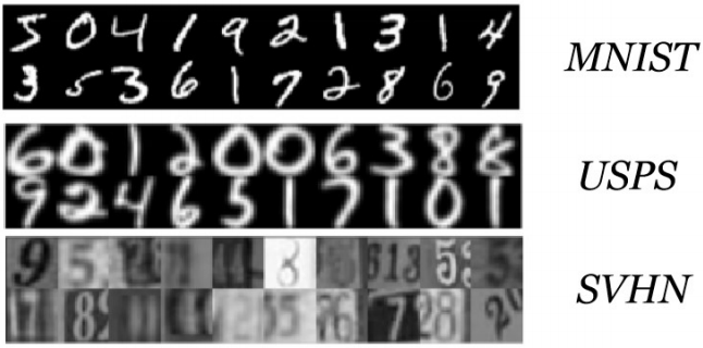
The SVHN dataset netzer2011reading has images from the street view house number from Google. This dataset is challenging due to changes in shape and textures, and extraneous numbers with the labeled image. It has over 600,000 digit images with ten classes. Fig. 33 shows sample images from MNIST, USPS, and SVHN dataset, respectively.

6.6 VisDA-2017

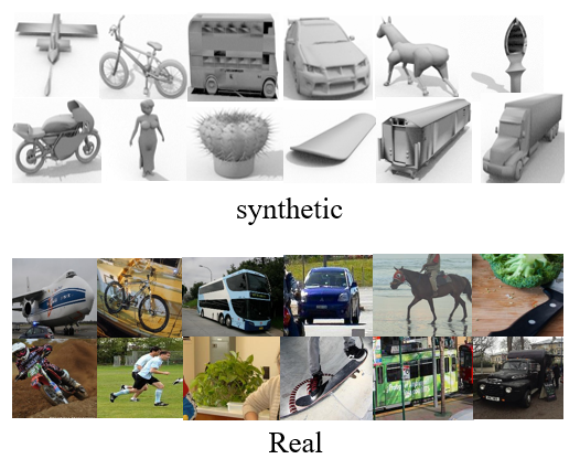
This dataset peng2017visda is closer to practical application scenarios and is a challenging dataset due to the significant domain-shift between the synthetic images (152,397 images from VisDA) and the real images (55,388 images from COCO) from 12 classes. The 12 classes are plane, bicycle, bus, car, horse, knife, motorcycle, person, plant, skateboard, train and truck as shown in Fig. 34.

Figure 34: Sample images of twelve classes from VisDA-2017 dataset (image from zhang2021unsupervised ).

6.7 ImageCLEF-DA

ImageCLEF-DA ImageCLEF-DA dataset is from ImageCLEF 2014 domain adaptation challenge. It contains three domains with a total of 600 images, which are formed by selecting images from three public datasets, including Caltech-256 (C), ImageNet ILSVRC 2012 (I), and Pascal VOC 2012 (P). Each domain consists of 12 categories, and each category contains 50 images. The 12 classes are aeroplane, bike, bird, boat, bottle, bus, car, dog, horse, monitor, motorbike, and people as shown in Fig. 35.

Figure 35: Sample images from four domains of the ImageCLEF-DA dataset. We only show images from four categories (image from zhang2021unsupervised ).

6.8 Amazon Reviews

Amazon Reviews blitzer2007biographies is a multi-domain sentiment dataset that contains product reviews taken from Amazon.com of four domains (Books, Kitchen, Electronics and DVDs). Each review in the four domains has a text and a rating from zero to five.

6.9 PIE

The Carnegie Mellon University (CMU) Pose, Illumination, and Expression (PIE) database Sim-2001-8175 contains 41,368 images of 68 people, where each person is represented under 13, 43, and 4, different poses, illuminations, and expressions, respectively. It has five subsets containing left pose, up pose, down pose, front pose, and right pose.

6.10 COIL20

Columbia Object Image Library (COIL20) Columbia is a dataset of 1,440 normalized images with 20 object categories. The images are at pose intervals of 5 degrees.

Table 1: Statistics of benchmark datasets

Dataset	$\#$ Sample	$\#$ Class	Domain(s)
Office-10	1,410	10	A, W, D
Caltech-10	1,123	10	C
Office-31	4,110	31	A, W, D
Office-Home	15,588	65	Ar, Cl, Pr, Rw
MNIST-USPS-SVHN	672,298	10	M, U, S
VisDA-2017	207,785	12	Synthetic, Real
ImageCLEF-DA	1,800	12	C, I, P
Amazon Reviews	8,000	2	B, K, E, D

Table 2: Statistics on PlantCLEF 2020 dataset

Domain	$\#$ Samples	$\#$ Classes
Herbarium (H)	320,750	997
Herbarium_photo_associations (A)	1,816	244
Photo (P)	4,482	375
Test (T)	3,186	-

Figure 36: Example images of the herbarium domain and photo domain. The large discrepancy between the two domains causes difficulty in improving the performance of the model (image from zhang2021unsupervised ).

Table 3: Accuracy (%) on Office + Caltech-10 (based on ResNet50)

Task	C$\shortrightarrow$A	C$\shortrightarrow$W	C$\shortrightarrow$D	A$\shortrightarrow$C	A$\shortrightarrow$W	A$\shortrightarrow$D	W$\shortrightarrow$C	W$\shortrightarrow$A	W$\shortrightarrow$D	D$\shortrightarrow$C	D$\shortrightarrow$A	D$\shortrightarrow$W	Ave.
GSM zhang2019transductive	96.0	95.9	96.2	94.6	89.5	92.4	94.1	95.8	100	93.9	95.1	98.6	95.2
BDA wang2017balanced	94.7	93.2	96.8	89.0	87.8	87.9	86.5	92.0	99.4	86.2	92.3	97.3	91.9
TJM long2014transfer	94.7	86.8	86.6	83.6	82.7	76.4	88.2	90.9	98.7	87.4	92.5	98.3	88.9
JGSA zhang2017joint	95.1	97.6	96.8	93.9	94.2	96.2	95.1	95.9	100	94.0	96.3	99.3	96.2
MEDA wang2018visual	96.3	98.3	96.2	94.6	99.0	100	94.8	96.6	100	93.6	96.0	99.3	97.0
DDC tzeng2014deep	91.9	85.4	88.8	85.0	86.1	89.0	78.0	83.8	100	79.0	87.1	97.7	86.1
DCORAL sun2016deep	89.8	97.3	91.0	91.9	100	90.5	83.7	81.5	90.1	88.6	80.1	92.3	89.7
DAN long2015learning	92.0	90.6	89.3	84.1	91.8	91.7	81.2	92.1	100	80.3	90.0	98.5	90.1
RTN long2016unsupervised	93.7	96.9	94.2	88.1	95.2	95.5	86.6	92.5	100	84.6	93.8	99.2	93.4
MDDA rahman2020minimum	93.6	95.2	93.4	89.1	95.7	96.6	86.5	94.8	100	84.7	94.7	99.4	93.6
DLSA zhang2021deep33	96.6	98.6	98.1	95.4	98.9	100	95.3	96.6	100	95.1	96.2	98.3	97.4

Table 4: Accuracy (%) on Office-Home dataset (based on ResNet50)

Task	Ar$\shortrightarrow$Cl	Ar$\shortrightarrow$Pr	Ar$\shortrightarrow$Rw	Cl$\shortrightarrow$Ar	Cl$\shortrightarrow$Pr	Cl$\shortrightarrow$Rw	Pr$\shortrightarrow$Ar	Pr$\shortrightarrow$Cl	Pr$\shortrightarrow$Rw	Rw$\shortrightarrow$Ar	Rw$\shortrightarrow$Cl	Rw$\shortrightarrow$Pr	Ave.
GSM zhang2019transductive	49.4	75.5	80.2	62.9	70.6	70.3	65.6	50.0	80.8	72.4	50.4	81.6	67.5
JGSA zhang2017joint	45.8	73.7	74.5	52.3	70.2	71.4	58.8	47.3	74.2	60.4	48.4	76.8	62.8
MEDA wang2018visual	49.1	75.6	79.1	66.7	77.2	75.8	68.2	50.4	79.9	71.9	53.2	82.0	69.1
ResNet-50 he2016deep	34.9	50.0	58.0	37.4	41.9	46.2	38.5	31.2	60.4	53.9	41.2	59.9	46.1
DAN long2015learning	43.6	57.0	67.9	45.8	56.5	60.4	44.0	43.6	67.7	63.1	51.5	74.3	56.3
DANN ghifary2014domain	45.6	59.3	70.1	47.0	58.5	60.9	46.1	43.7	68.5	63.2	51.8	76.8	57.6
JAN long2017deep	45.9	61.2	68.9	50.4	59.7	61.0	45.8	43.4	70.3	63.9	52.4	76.8	58.3
CDAN-M long2018conditional	50.6	65.9	73.4	55.7	62.7	64.2	51.8	49.1	74.5	68.2	56.9	80.7	62.8
TAT liu2019transferable	51.6	69.5	75.4	59.4	69.5	68.6	59.5	50.5	76.8	70.9	56.6	81.6	65.8
ETD li2020enhanced	51.3	71.9	85.7	57.6	69.2	73.7	57.8	51.2	79.3	70.2	57.5	82.1	67.3
TADA wang2019transferable	53.1	72.3	77.2	59.1	71.2	72.1	59.7	53.1	78.4	72.4	60.0	82.9	67.6
SymNets zhang2019domain	47.7	72.9	78.5	64.2	71.3	74.2	64.2	48.8	79.5	74.5	52.6	82.7	67.6
DCAN li2020domain	54.5	75.7	81.2	67.4	74.0	76.3	67.4	52.7	80.6	74.1	59.1	83.5	70.5
RSDA gu2020spherical	53.2	77.7	81.3	66.4	74.0	76.5	67.9	53.0	82.0	75.8	57.8	85.4	70.9
SPL wang2020unsupervised	54.5	77.8	81.9	65.1	78.0	81.1	66.0	53.1	82.8	69.9	55.3	86.0	71.0
ESD zhang2021enhanced	53.2	75.9	82.0	68.4	79.3	79.4	69.2	54.8	81.9	74.6	56.2	83.8	71.6
DLSA zhang2021deep33	56.3	79.4	82.5	67.4	78.4	78.6	69.4	54.5	82.1	75.3	56.4	83.7	71.7
SHOT liang2020we	57.1	78.1	81.5	68.0	78.2	78.1	67.4	54.9	82.2	73.3	58.8	84.3	71.8

Table 5: Accuracy (%) on VisDA-2017 dataset (based on ResNet101)

Task	plane	bcycl	bus	car	horse	knife	mcycl	person	plant	sktbrd	train	truck	Ave.
Source-only he2016deep	55.1	53.3	61.9	59.1	80.6	17.9	79.7	31.2	81.0	26.5	73.5	8.5	52.4
DANN ghifary2014domain	81.9	77.7	82.8	44.3	81.2	29.5	65.1	28.6	51.9	54.6	82.8	7.8	57.4
DAN long2015learning	87.1	63.0	76.5	42.0	90.3	42.9	85.9	53.1	49.7	36.3	85.8	20.7	61.1
JAN long2017deep	75.7	18.7	82.3	86.3	70.2	56.9	80.5	53.8	92.5	32.2	84.5	54.5	65.7
MCD saito2018maximum	87.0	60.9	83.7	64.0	88.9	79.6	84.7	76.9	88.6	40.3	83.0	25.8	71.9
DMP luo2020unsupervised	92.1	75.0	78.9	75.5	91.2	81.9	89.0	77.2	93.3	77.4	84.8	35.1	79.3
DADA tang2020discriminative	92.9	74.2	82.5	65.0	90.9	93.8	87.2	74.2	89.9	71.5	86.5	48.7	79.8
STAR lu2020stochastic	95.0	84.0	84.6	73.0	91.6	91.8	85.9	78.4	94.4	84.7	87.0	42.2	82.7
SHOT liang2020we	94.3	88.5	80.1	57.3	93.1	94.9	80.7	80.3	91.5	89.1	86.3	58.2	82.9
DSGK zhang2021deep	95.7	86.3	85.8	77.3	92.3	94.9	88.5	82.9	94.9	86.5	88.1	46.8	85.0
CAN kang2019contrastive	97.9	87.2	82.5	74.3	97.8	96.2	90.8	80.7	96.6	96.3	87.5	59.9	87.2
DLSA zhang2021deep33	96.9	89.2	85.4	77.9	98.3	96.9	91.3	82.6	96.9	96.5	88.3	60.8	88.4

Table 6: Accuracy (%) on Office-31 (ResNet50)

Task	A$\shortrightarrow$W	A$\shortrightarrow$D	W$\shortrightarrow$A	W$\shortrightarrow$D	D$\shortrightarrow$A	D$\shortrightarrow$W	Ave.
GSM zhang2019transductive	85.9	84.1	75.5	97.2	73.6	95.6	85.3
BDA wang2017balanced	77.0	79.3	70.3	97.0	68.0	93.2	80.8
JGSA zhang2017joint	89.1	91.0	77.9	100	77.6	98.2	89.0
MEDA wang2018visual	91.7	89.2	77.2	97.4	76.5	96.2	88.0
RTN long2016unsupervised	84.5	77.5	64.8	99.4	66.2	96.8	81.6
ADDA tzeng2017adversarial	86.2	77.8	68.9	98.4	69.5	96.2	82.9
JAN long2017deep	85.4	84.7	70.0	99.8	68.6	97.4	84.3
DMRL wu2020dual	90.8	93.4	71.2	100	73.0	99.0	87.9
TAT liu2019transferable	92.5	93.2	73.1	100	73.1	99.3	88.4
TADA wang2019transferable	94.3	91.6	73.0	99.8	72.9	98.7	88.4
SymNets zhang2019domain	90.8	93.9	72.5	100	74.6	98.8	88.4
SHOT liang2020we	90.1	94.0	74.3	99.9	74.7	98.4	88.6
SPL wang2020unsupervised	92.7	93.0	76.8	99.8	76.4	98.7	89.6
CAN kang2019contrastive	94.5	95.0	77.0	99.8	78.0	99.1	90.6
RSDA gu2020spherical	96.1	95.8	78.9	100	77.4	99.3	91.3
DLSA zhang2021deep33	95.2	96.2	80.4	99.2	80.7	98.0	91.6

6.11 PlantCLEF 2020

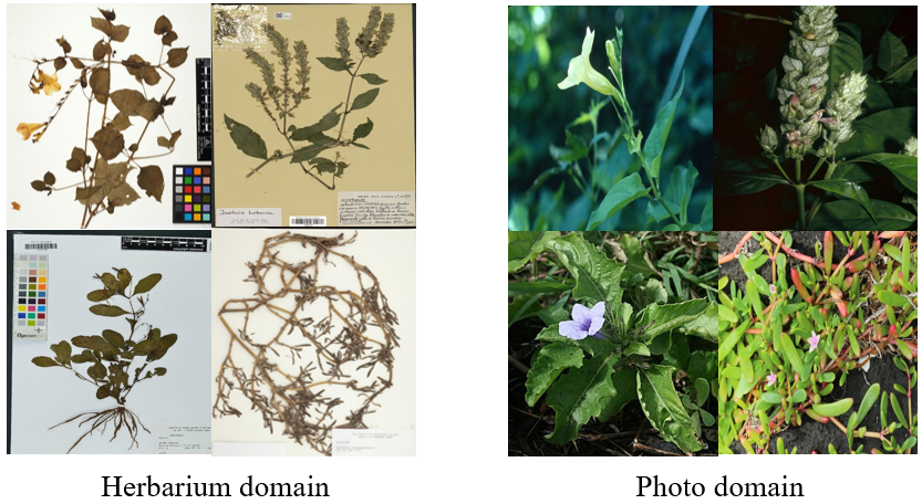
This dataset is a large-scale dataset of the PlantCLEF 2020 task plantclef2020 . Fig. 36 shows some challenging images in this dataset. Tab. 2 lists the statistics on PlantCLEF 2021 dataset. The herbarium domain contains 320,750 images in 997 species, and the number of images in different species are unbalanced. This dataset consists of herbarium sheets whereas the test set will be composed of field pictures. The validation set consists of two domains herbarium_photo_associations and photos. Herbarium_photo_associations domain includes 1,816 images from 244 species. This domain contains both herbarium sheets and field pictures for a subset of species, which enables learning a mapping between the herbarium sheets domain and the field pictures domain. Another photo domain has 4,482 images from 375 species and images are from plant pictures in the field, which is similar to the test dataset. The test dataset contains 3,186 unlabeled images. Due to the significant difference between herbarium and real photos, it is extremely difficult to identify the correct class zhang2020adversarial1 ; zhang2021weighted .

6.12 State-of-the-art results of image recognition

As shown in Tab. 3-Tab. 6, we provide the results of four benchmark datasets (Office + Caltech-10, Office-31, Office-Home and VisDA-2017). In this experiment, C $\shortrightarrow$ A means learning from existing domain C, and transferring knowledge to classify domain A. These results indicate that deep learning-based methods usually achieve better performance than traditional methods. However, some traditional methods (wang2018visual ; zhang2019modified ) observe higher accuracy than some deep learning-based methods. This is mainly because the extracted features are from pre-trained deep neural networks. Therefore, there is a trend of combining traditional based methods with deep learning features. Also, deep learning models with pseudo-labeling techniques achieve promising results.

7 Conclusions

In this survey, we first introduce some basic notation for unsupervised domain adaptation, then review existing research in the context of UDA and describe benchmark datasets with some state-of-the-art performance. We focus on two categories of image recognition methods: traditional methods and deep learning based methods.

Traditional methods rely on different feature extraction techniques to better represent images of the two domains. We discuss these methods from three directions: feature selection, distribution alignment, and subspace learning. Specifically, we illustrate three settings of distribution alignment: marginal, conditional, and joint distribution alignment.

We present the deep learning based UDA from six directions: discrepancy-based, adversarial-based, pseudo-labeling-based, reconstruction-based, representation-based, and attention-based methods. Specifically, we review eight different discrepancy based methods: maximum mean discrepancy, correlation alignment, Kullback–Leibler divergence, Jensen–Shannon divergence, Wasserstein distance, mutual information, entropy minimization, batch normalization, and least squares estimation.

Although both traditional and deep learning-based methods have been proposed to solve the domain shift issue, they both have some limitations. Traditional methods heavily rely on the extracted deep features from well-trained neural networks to achieve better performance. Deep learning-based methods usually take a long computation time to train the images from scratch. In real-world applications, how to better extract deep features from images and design incremental and online UDA algorithms can be promising directions.

References

- [1] L. Chen, H. Zhang, J. Xiao, W. Liu, and S.-F. Chang. Zero-shot visual recognition using semantics-preserving adversarial embedding network. In Proceedings of the IEEE Conference on Computer Vision and Pattern Recognition, volume 2, 2018.
- [2] M. Long, J. Wang, G. Ding, J. Sun, and P. S. Yu. Transfer joint matching for unsupervised domain adaptation. In Proceedings of the IEEE Conference on Computer Vision and Pattern Recognition, pages 1410–1417, 2014.
- [3] Y. Zhang. Unsupervised Domain Adaptation for Visual Recognition. PhD thesis, Lehigh University, 2021.
- [4] J. Deng, W. Dong, R. Socher, L.-J. Li, K. Li, and F.-F. Li. Imagenet: A large-scale hierarchical image database. In 2009 IEEE conference on computer vision and pattern recognition, pages 248–255. Ieee, 2009.
- [5] A. Krizhevsky and G. Hinton. Convolutional deep belief networks on cifar-10. Unpublished manuscript, 40(7):1–9, 2010.
- [6] S. J. Pan and Q. Yang. A survey on transfer learning. IEEE Transactions on knowledge and data engineering, 22(10):1345–1359, 2010.
- [7] A. Krizhevsky, I. Sutskever, and G. E. Hinton. ImageNet classification with deep convolutional neural networks. In Advances in Neural Information Processing Systems, pages 1097–1105, 2012.
- [8] M. Long, H. Zhu, J. Wang, and M. I. Jordan. Deep transfer learning with joint adaptation networks. In Proceedings of the 34th International Conference on Machine Learning, volume 70, pages 2208–2217. JMLR.org, 2017.
- [9] Y. Zhang, S. Xie, and B. D. Davison. Transductive learning via improved geodesic sampling. In Proceedings of the 30th British Machine Vision Conference, 2019.
- [10] Y. Zhang and B. D. Davison. Modified distribution alignment for domain adaptation with pre-trained InceptionResNet. arXiv preprint arXiv:1904.02322, 2019.
- [11] Y. Zhang and B. D. Davison. Impact of imagenet model selection on domain adaptation. In Proceedings of the IEEE Winter Conference on Applications of Computer Vision Workshops, pages 173–182, 2020.
- [12] E. Tzeng, J. Hoffman, K. Saenko, and T. Darrell. Adversarial discriminative domain adaptation. In Proceedings of the IEEE Conference on Computer Vision and Pattern Recognition, pages 7167–7176, 2017.
- [13] H. Liu, M. Long, J. Wang, and M. Jordan. Transferable adversarial training: A general approach to adapting deep classifiers. In International Conference on Machine Learning, pages 4013–4022, 2019.
- [14] L. Shao, F. Zhu, and X. Li. Transfer learning for visual categorization: A survey. IEEE transactions on neural networks and learning systems, 26(5):1019–1034, 2015.
- [15] O. Day and T. M. Khoshgoftaar. A survey on heterogeneous transfer learning. Journal of Big Data, 4(1):29, 2017.
- [16] V. M. Patel, R. Gopalan, R. Li, and R. Chellappa. Visual domain adaptation: A survey of recent advances. IEEE signal processing magazine, 32(3):53–69, 2015.
- [17] J. Zhang, W. Li, and P. Ogunbona. Transfer learning for cross-dataset recognition: a survey. arXiv preprint arXiv:1705.04396, 2017.
- [18] G. Csurka. Domain adaptation for visual applications: A comprehensive survey. arXiv preprint arXiv:1702.05374, 2017.
- [19] M. Wang and W. Deng. Deep visual domain adaptation: A survey. Neurocomputing, 312:135–153, 2018.
- [20] S. Ben-David, J. Blitzer, K. Crammer, A. Kulesza, F. Pereira, and J. W. Vaughan. A theory of learning from different domains. Machine Learning, 79(1-2):151–175, 2010.
- [21] H. Bay, T. Tuytelaars, and L. Van Gool. Surf: Speeded up robust features. In European conference on computer vision, pages 404–417. Springer, 2006.
- [22] J. Blitzer, R. McDonald, and F. Pereira. Domain adaptation with structural correspondence learning. In Proc. Empirical Methods in Natural Language Processing, pages 120–128, 2006.
- [23] E. Rashedi, H. Nezamabadi-Pour, and S. Saryazdi. A simultaneous feature adaptation and feature selection method for content-based image retrieval systems. Knowledge-Based Systems, 39:85–94, 2013.
- [24] J. Li, J. Zhao, and K. Lu. Joint feature selection and structure preservation for domain adaptation. In IJCAI, pages 1697–1703, 2016.
- [25] Q. Gu, Z. Li, and J. Han. Joint feature selection and subspace learning. In Twenty-Second International Joint Conference on Artificial Intelligence, 2011.
- [26] Y. Zhang, J. P. Allem, J. B. Unger, and T. B. Cruz. Automated identification of hookahs (waterpipes) on instagram: an application in feature extraction using convolutional neural network and support vector machine classification. Journal of Medical Internet Research, 20(11):e10513, 2018.
- [27] Y. Zhang and Q. Li. A regressive convolution neural network and support vector regression model for electricity consumption forecasting. In Future of Information and Communication Conference, pages 33–45. Springer, 2019.
- [28] Y. Wu and Y. Zhang. Mixing deep visual and textual features for image regression. In Proceedings of SAI Intelligent Systems Conference, pages 747–760. Springer, 2020.
- [29] Y. Zhang and B. D. Davison. Efficient pre-trained features and recurrent pseudo-labeling in unsupervised domain adaptation. In Proceedings of the IEEE/CVF Conference on Computer Vision and Pattern Recognition Workshops (CVPRW), pages 2719–2728, 2021.
- [30] S. J. Pan, I. W. Tsang, J. T. Kwok, and Q. Yang. Domain adaptation via transfer component analysis. IEEE Trans. on Neural Networks, 22(2):199–210, 2011.
- [31] F. Dorri and A. Ghodsi. Adapting component analysis. In 2012 IEEE 12th International Conference on Data Mining, pages 846–851. IEEE, 2012.
- [32] M. Baktashmotlagh, M. Harandi, and M. Salzmann. Distribution-matching embedding for visual domain adaptation. The Journal of Machine Learning Research, 17(1):3760–3789, 2016.
- [33] M. Jiang, W. Huang, Z. Huang, and G. G. Yen. Integration of global and local metrics for domain adaptation learning via dimensionality reduction. IEEE Transactions on Cybernetics, 47(1):38–51, 2017.
- [34] L. Duan, I. W. Tsang, and D. Xu. Domain transfer multiple kernel learning. IEEE Transactions on Pattern Analysis and Machine Intelligence, 34(3):465–479, 2012.
- [35] M. Gong, K. Zhang, T. Liu, D. Tao, C. Glymour, and B. Schölkopf. Domain adaptation with conditional transferable components. In Proc. International Conference on Machine Learning, pages 2839–2848, 2016.
- [36] S. Satpal and S. Sarawagi. Domain adaptation of conditional probability models via feature subsetting. In European Conference on Principles of Data Mining and Knowledge Discovery, pages 224–235. Springer, 2007.
- [37] J. Wang, Y. Chen, L. Hu, X. Peng, and P. S. Yu. Stratified transfer learning for cross-domain activity recognition. In 2018 IEEE International Conference on Pervasive Computing and Communications (PerCom), pages 1–10. IEEE, 2018.
- [38] M. Long, J. Wang, G. Ding, J. Sun, and P. S. Yu. Transfer feature learning with joint distribution adaptation. In Proceedings of the IEEE International Conference on Computer Vision, pages 2200–2207, 2013.
- [39] M. Long, J. Wang, G. Ding, S. J. Pan, and S. Y. Philip. Adaptation regularization: A general framework for transfer learning. IEEE Transactions on Knowledge and Data Engineering, 26(5):1076–1089, 2013.
- [40] J. Tahmoresnezhad and S. Hashemi. Visual domain adaptation via transfer feature learning. Knowledge and Information Systems, 50(2):585–605, 2017.
- [41] P.-H. Hsiao, F.-J. Chang, and Y.-Y. Lin. Learning discriminatively reconstructed source data for object recognition with few examples. IEEE Transactions on Image Processing, 25(8):3518–3532, 2016.
- [42] C.-A. Hou, Y.-R. Yeh, and Y.-C. F. Wang. An unsupervised domain adaptation approach for cross-domain visual classification. In 2015 12th IEEE International Conference on Advanced Video and Signal Based Surveillance (AVSS), pages 1–6. IEEE, 2015.
- [43] J. Zhang, W. Li, and P. Ogunbona. Joint geometrical and statistical alignment for visual domain adaptation. In Proceedings of the IEEE Conference on Computer Vision and Pattern Recognition, pages 1859–1867, 2017.
- [44] J. Wang, Y. Chen, S. Hao, W. Feng, and Z. Shen. Balanced distribution adaptation for transfer learning. In Proceedings of the IEEE International Conference on Data Mining (ICDM), pages 1129–1134, 2017.
- [45] J. Wang, W. Feng, Y. Chen, H. Yu, M. Huang, and P. S. Yu. Visual domain adaptation with manifold embedded distribution alignment. In Proceedings of the 26th ACM International Conference on Multimedia, MM ’18, pages 402–410, 2018.
- [46] C. Wang and S. Mahadevan. Manifold alignment without correspondence. In IJCAI, volume 2, page 3, 2009.
- [47] B. Gong, Y. Shi, F. Sha, and K. Grauman. Geodesic flow kernel for unsupervised domain adaptation. In IEEE Conference on Computer Vision and Pattern Recognition (CVPR), pages 2066–2073. IEEE, 2012.
- [48] Y. Zhang and B. D. Davison. Correlated adversarial joint discrepancy adaptation network. In 2021 International Conference on Content-Based Multimedia Indexing (CBMI), pages 1–6, 2021.
- [49] B. Fernando, A. Habrard, M. Sebban, and T. Tuytelaars. Unsupervised visual domain adaptation using subspace alignment. In Proceedings of the IEEE international conference on computer vision, pages 2960–2967, 2013.
- [50] B. Sun and K. Saenko. Subspace distribution alignment for unsupervised domain adaptation. In BMVC, volume 4, pages 24–1, 2015.
- [51] B. Sun, J. Feng, and K. Saenko. Return of frustratingly easy domain adaptation. In Thirtieth AAAI Conference on Artificial Intelligence, 2016.
- [52] S. J. Pan, X. Ni, J.-T. Sun, Q. Yang, and Z. Chen. Cross-domain sentiment classification via spectral feature alignment. In Proceedings of the 19th international conference on World wide web, pages 751–760, 2010.
- [53] R. Gopalan, R. Li, and R. Chellappa. Domain adaptation for object recognition: An unsupervised approach. In IEEE International Conference on Computer Vision (ICCV), pages 999–1006. IEEE, 2011.
- [54] Y. Zhang and B. D. Davison. Domain adaptation for object recognition using subspace sampling demons. Multimedia Tools and Applications, 2020.
- [55] Y. Zhang and B. D Davison. Deep spherical manifold gaussian kernel for unsupervised domain adaptation. In Proceedings of the IEEE/CVF Conference on Computer Vision and Pattern Recognition Workshops, pages 4443–4452, 2021.
- [56] E. Tzeng, J. Hoffman, N. Zhang, K. Saenko, and T. Darrell. Deep domain confusion: Maximizing for domain invariance. arXiv preprint arXiv:1412.3474, 2014.
- [57] E. Tzeng, J. Hoffman, T. Darrell, and K. Saenko. Simultaneous deep transfer across domains and tasks. In Proceedings of the IEEE International Conference on Computer Vision, pages 4068–4076, 2015.
- [58] M. Long, Y. Cao, J. Wang, and M. I. Jordan. Learning transferable features with deep adaptation networks. arXiv preprint arXiv:1502.02791, 2015.
- [59] M. Long, H. Zhu, J. Wang, and M. I. Jordan. Unsupervised domain adaptation with residual transfer networks. In Advances in Neural Information Processing Systems, pages 136–144, 2016.
- [60] H. Yan, Y. Ding, P. Li, Q. Wang, Y. Xu, and W. Zuo. Mind the class weight bias: Weighted maximum mean discrepancy for unsupervised domain adaptation. In Proceedings of the IEEE Conference on Computer Vision and Pattern Recognition, pages 2272–2281, 2017.
- [61] Y. Zhu, F. Zhuang, J. Wang, J. Chen, Z. Shi, W. Wu, and Q. He. Multi-representation adaptation network for cross-domain image classification. Neural Networks, 119:214–221, 2019.
- [62] G. Kang, L. Jiang, Y. Yang, and A. G. Hauptmann. Contrastive adaptation network for unsupervised domain adaptation. In Proceedings of the IEEE Conference on Computer Vision and Pattern Recognition, pages 4893–4902, 2019.
- [63] W. Deng, L. Zheng, Y. Sun, and J. Jiao. Rethinking triplet loss for domain adaptation. IEEE Transactions on Circuits and Systems for Video Technology, 2020.
- [64] B. Sun and K. Saenko. Deep CORAL: Correlation alignment for deep domain adaptation. In European Conference on Computer Vision, pages 443–450. Springer, 2016.
- [65] Y. Zhang, N. Wang, S. Cai, and L. Song. Unsupervised domain adaptation by mapped correlation alignment. IEEE Access, 6:44698–44706, 2018.
- [66] C. Chen, Z. Chen, B. Jiang, and X. Jin. Joint domain alignment and discriminative feature learning for unsupervised deep domain adaptation. In Proceedings of the AAAI Conference on Artificial Intelligence, volume 33, pages 3296–3303, 2019.
- [67] M. M. Rahman, C. Fookes, M. Baktashmotlagh, and S. Sridharan. On minimum discrepancy estimation for deep domain adaptation. In Domain Adaptation for Visual Understanding, pages 81–94. Springer, 2020.
- [68] T. Van Erven and P. Harremos. Rényi divergence and kullback-leibler divergence. IEEE Transactions on Information Theory, 60(7):3797–3820, 2014.
- [69] F. Zhuang, X. Cheng, P. Luo, S. J. Pan, and Q. He. Supervised representation learning with double encoding-layer autoencoder for transfer learning. ACM Transactions on Intelligent Systems and Technology (TIST), 9(2):1–17, 2017.
- [70] Z. Meng, J. Li, Y. Gong, and B. Juang. Adversarial teacher-student learning for unsupervised domain adaptation. In 2018 IEEE International Conference on Acoustics, Speech and Signal Processing (ICASSP), pages 5949–5953. IEEE, 2018.
- [71] B. Fuglede and F. Topsoe. Jensen-shannon divergence and hilbert space embedding. In International Symposium onInformation Theory, 2004. ISIT 2004. Proceedings., page 31. IEEE, 2004.
- [72] J. Jiang, X. Wang, M. Long, and J. Wang. Resource efficient domain adaptation. In Proceedings of the 28th ACM International Conference on Multimedia, pages 2220–2228, 2020.
- [73] C.-Y. Lee, T. Batra, M. H. Baig, and D. Ulbricht. Sliced wasserstein discrepancy for unsupervised domain adaptation. In Proceedings of the IEEE Conference on Computer Vision and Pattern Recognition, pages 10285–10295, 2019.
- [74] S. S. Vallender. Calculation of the wasserstein distance between probability distributions on the line. Theory of Probability & Its Applications, 18(4):784–786, 1974.
- [75] B. B. Damodaran, B. Kellenberger, R. Flamary, D. Tuia, and N. Courty. Deepjdot: Deep joint distribution optimal transport for unsupervised domain adaptation. In Proceedings of the European Conference on Computer Vision (ECCV), pages 447–463, 2018.
- [76] A. Kraskov, H. Stögbauer, and P. Grassberger. Estimating mutual information. Physical review E, 69(6):066138, 2004.
- [77] B. Gholami, P. Sahu, O. Rudovic, K. Bousmalis, and V. Pavlovic. Unsupervised multi-target domain adaptation: An information theoretic approach. IEEE Transactions on Image Processing, 29:3993–4002, 2020.
- [78] X. Xie, J. Chen, Y. Li, L. Shen, K. Ma, and Y. Zheng. Mi2gan: Generative adversarial network for medical image domain adaptation using mutual information constraint. In International Conference on Medical Image Computing and Computer-Assisted Intervention, pages 516–525. Springer, 2020.
- [79] Y. Grandvalet and Y. Bengio. Semi-supervised learning by entropy minimization. CAP, 367:281–296, 2005.
- [80] K. Sohn, W. Shang, X. Yu, and M. Chandraker. Unsupervised domain adaptation for distance metric learning. In International Conference on Learning Representations, 2018.
- [81] S. Roy, A. Siarohin, E. Sangineto, S. R. Bulo, N. Sebe, and E. Ricci. Unsupervised domain adaptation using feature-whitening and consensus loss. In Proceedings of the IEEE Conference on Computer Vision and Pattern Recognition, pages 9471–9480, 2019.
- [82] M. Mancini, L. Porzi, S. Rota Bulò, B. Caputo, and E. Ricci. Boosting domain adaptation by discovering latent domains. In Proceedings of the IEEE Conference on Computer Vision and Pattern Recognition, pages 3771–3780, 2018.
- [83] S. Ioffe and C. Szegedy. Batch normalization: Accelerating deep network training by reducing internal covariate shift. arXiv preprint arXiv:1502.03167, 2015.
- [84] Y. Li, N. Wang, J. Shi, X. Hou, and J. Liu. Adaptive batch normalization for practical domain adaptation. Pattern Recognition, 80:109–117, 2018.
- [85] W.-G. Chang, T. You, S. Seo, S. Kwak, and B. Han. Domain-specific batch normalization for unsupervised domain adaptation. In Proceedings of the IEEE Conference on Computer Vision and Pattern Recognition, pages 7354–7362, 2019.
- [86] Y. Zhang and B. D. Davison. Deep least squares alignment for unsupervised domain adaptation. In Proceedings of the 32th British Machine Vision Conference, 2021.
- [87] I. Goodfellow, J. Pouget-Abadie, M. Mirza, B. Xu, D. Warde-Farley, S. Ozair, A. Courville, and Y. Bengio. Generative adversarial nets. In Advances in neural information processing systems, pages 2672–2680, 2014.
- [88] M. Long, Z. Cao, J. Wang, and M. I. Jordan. Conditional adversarial domain adaptation. In Advances in Neural Information Processing Systems, pages 1647–1657, 2018.
- [89] Y. Zhang, H. Tang, K. Jia, and M. Tan. Domain-symmetric networks for adversarial domain adaptation. In Proceedings of the IEEE Conference on Computer Vision and Pattern Recognition, pages 5031–5040, 2019.
- [90] G. Wei, C. Lan, W. Zeng, and Z. Chen. Metaalign: Coordinating domain alignment and classification for unsupervised domain adaptation. In Proceedings of the IEEE/CVF Conference on Computer Vision and Pattern Recognition, pages 16643–16653, 2021.
- [91] A. Ma, J. Li, K. Lu, L. Zhu, and H. T. Shen. Adversarial entropy optimization for unsupervised domain adaptation. IEEE Transactions on Neural Networks and Learning Systems, 2021.
- [92] T. Jing and Z. Ding. Adversarial dual distinct classifiers for unsupervised domain adaptation. In Proceedings of the IEEE/CVF Winter Conference on Applications of Computer Vision, pages 605–614, 2021.
- [93] I. B. Akkaya, F. Altinel, and U. Halici. Self-training guided adversarial domain adaptation for thermal imagery. In Proceedings of the IEEE/CVF Conference on Computer Vision and Pattern Recognition, pages 4322–4331, 2021.
- [94] Y. Zhang, H. Ye, and B. D. Davison. Adversarial reinforcement learning for unsupervised domain adaptation. In Proceedings of the IEEE/CVF Winter Conference on Applications of Computer Vision, pages 635–644, 2021.
- [95] Y. Zhang and B. D. Davison. Adversarial regression learning for bone age estimation. In International Conference on Information Processing in Medical Imaging, pages 742–754. Springer, 2021.
- [96] Y. Ganin, E. Ustinova, H. Ajakan, P. Germain, H. Larochelle, F. Laviolette, M. Marchand, and V. Lempitsky. Domain-adversarial training of neural networks. The Journal of Machine Learning Research, 17(1):2096–2030, 2016.
- [97] M.-Y. Liu and O. Tuzel. Coupled generative adversarial networks. In Advances in neural information processing systems, pages 469–477, 2016.
- [98] Z. Cao, L. Ma, M. Long, and J. Wang. Partial adversarial domain adaptation. In Proceedings of the European Conference on Computer Vision (ECCV), pages 135–150, 2018.
- [99] W. Zhang, W. Ouyang, W. Li, and D. Xu. Collaborative and adversarial network for unsupervised domain adaptation. In Proceedings of the IEEE Conference on Computer Vision and Pattern Recognition, pages 3801–3809, 2018.
- [100] M. Li, Y.-M. Zhai, Y.-W. Luo, P.-F. Ge, and C.-X. Ren. Enhanced transport distance for unsupervised domain adaptation. In Proceedings of the IEEE/CVF Conference on Computer Vision and Pattern Recognition, pages 13936–13944, 2020.
- [101] J. Hoffman, E. Tzeng, T. Park, J.-Y. Zhu, P. Isola, K. Saenko, A. Efros, and T. Darrell. Cycada: Cycle-consistent adversarial domain adaptation. In International conference on machine learning, pages 1989–1998. PMLR, 2018.
- [102] H.-K. Hsu, C.-H. Yao, Y.-H. Tsai, W.-C. Hung, H.-Y. Tseng, M. Singh, and M.-H. Yang. Progressive domain adaptation for object detection. In The IEEE Winter Conference on Applications of Computer Vision, pages 749–757, 2020.
- [103] T. Miyato, S. Maeda, M. Koyama, and S. Ishii. Virtual adversarial training: a regularization method for supervised and semi-supervised learning. IEEE transactions on pattern analysis and machine intelligence, 41(8):1979–1993, 2018.
- [104] R. Shu, H. H. Bui, H. Narui, and S. Ermon. A dirt-t approach to unsupervised domain adaptation. arXiv preprint arXiv:1802.08735, 2018.
- [105] M. Xu, B. Zhang, J.and Ni, T. Li, C. Wang, Q. Tian, and W. Zhang. Adversarial domain adaptation with domain mixup. arXiv preprint arXiv:1912.01805, 2019.
- [106] C. Zhang, Q. Zhao, and Y. Wang. Hybrid adversarial network for unsupervised domain adaptation. Information Sciences, 514:44–55, 2020.
- [107] K. Saito, Y. Ushiku, and T. Harada. Asymmetric tri-training for unsupervised domain adaptation. arXiv preprint arXiv:1702.08400, 2017.
- [108] S. Xie, Z. Zheng, L. Chen, and C. Chen. Learning semantic representations for unsupervised domain adaptation. In International Conference on Machine Learning, pages 5423–5432, 2018.
- [109] C. Chen, W. Xie, W. Huang, Y. Rong, X. Ding, Y. Huang, T. Xu, and J. Huang. Progressive feature alignment for unsupervised domain adaptation. In Proc. IEEE Conf. on Computer Vision and Pattern Recognition, pages 627–636, 2019.
- [110] Y. Zhang and B. D. Davison. Adversarial continuous learning on unsupervised domain adaptation. In 25th International Conference on Pattern Recognition Workshops, pages 672–687, 2020.
- [111] Y. Zhang, B. Deng, K. Jia, and L. Zhang. Label propagation with augmented anchors: A simple semi-supervised learning baseline for unsupervised domain adaptation. In European Conference on Computer Vision, pages 781–797. Springer, 2020.
- [112] K. Bousmalis, G. Trigeorgis, N. Silberman, D. Krishnan, and D. Erhan. Domain separation networks. In Advances in Neural Information Processing Systems, pages 343–351, 2016.
- [113] M. Ghifary, W. B. Kleijn, M. Zhang, D. Balduzzi, and W. Li. Deep reconstruction-classification networks for unsupervised domain adaptation. In European Conference on Computer Vision, pages 597–613. Springer, 2016.
- [114] P. Vincent, H. Larochelle, Y. Bengio, and P.-A. Manzagol. Extracting and composing robust features with denoising autoencoders. In Proceedings of the 25th international conference on Machine learning, pages 1096–1103. ACM, 2008.
- [115] M. Chen, Z. E. Xu, K. Q. Weinberger, and F. Sha. Marginalized denoising autoencoders for domain adaptation. In ICML, 2012.
- [116] M. Ghifary, W. Bastiaan Kleijn, M. Zhang, and D. Balduzzi. Domain generalization for object recognition with multi-task autoencoders. In Proceedings of the IEEE international conference on computer vision, pages 2551–2559, 2015.
- [117] F. Zhuang, X. Cheng, P. Luo, S. J. Pan, and Q. He. Supervised representation learning: Transfer learning with deep autoencoders. In Twenty-Fourth International Joint Conference on Artificial Intelligence, 2015.
- [118] Y.-C. Liu, Y.-Y. Yeh, T.-C. Fu, S.-D. Wang, W.-C. Chiu, and Y.-C. Frank Wang. Detach and adapt: Learning cross-domain disentangled deep representation. In Proceedings of the IEEE Conference on Computer Vision and Pattern Recognition, pages 8867–8876, 2018.
- [119] A. Gonzalez-Garcia, J. Van De Weijer, and Y. Bengio. Image-to-image translation for cross-domain disentanglement. Advances in neural information processing systems, 31:1287–1298, 2018.
- [120] A. H. Liu, Y.-C. Liu, Y.-Y. Yeh, and Y. F. Wang. A unified feature disentangler for multi-domain image translation and manipulation. In Advances in neural information processing systems, pages 2590–2599, 2018.
- [121] X. Peng, Z. Huang, X. Sun, and K. Saenko. Domain agnostic learning with disentangled representations. In International Conference on Machine Learning, pages 5102–5112, 2019.
- [122] Y. Zhang and B. D. Davison. Enhanced separable disentanglement for unsupervised domain adaptation. In 2021 IEEE International Conference on Image Processing, pages 784–788, 2021.
- [123] F. Wang, M. Jiang, C. Qian, S. Yang, C. Li, H. Zhang, X. Wang, and X. Tang. Residual attention network for image classification. In Proceedings of the IEEE conference on computer vision and pattern recognition, pages 3156–3164, 2017.
- [124] J. Zhuo, S. Wang, W. Zhang, and Q. Huang. Deep unsupervised convolutional domain adaptation. In Proceedings of the 25th ACM international conference on Multimedia, pages 261–269, 2017.
- [125] S. Moon and J. G. Carbonell. Completely heterogeneous transfer learning with attention-what and what not to transfer. In IJCAI, pages 1–2, 2017.
- [126] G. Kang, L. Zheng, Y. Yan, and Y. Yang. Deep adversarial attention alignment for unsupervised domain adaptation: the benefit of target expectation maximization. In Proceedings of the European Conference on Computer Vision (ECCV), pages 401–416, 2018.
- [127] K. Saenko, B. Kulis, M. Fritz, and T. Darrell. Adapting visual category models to new domains. In European conference on computer vision, pages 213–226. Springer, 2010.
- [128] H. Venkateswara, J. Eusebio, S. Chakraborty, and S. Panchanathan. Deep hashing network for unsupervised domain adaptation. In Proceedings of the IEEE Conference on Computer Vision and Pattern Recognition, pages 5018–5027, 2017.
- [129] Y. LeCun, L. Bottou, Y. Bengio, and P. Haffner. Gradient-based learning applied to document recognition. Proceedings of the IEEE, 86(11):2278–2324, 1998.
- [130] J. Friedman, T. Hastie, and R. Tibshirani. The elements of statistical learning. Number 10. Springer series in statistics New York, 2001.
- [131] Y. Netzer, T. Wang, A. Coates, A. Bissacco, B. Wu, and A. Y. Ng. Reading digits in natural images with unsupervised feature learning. 2011.
- [132] X. Peng, B. Usman, N. Kaushik, J. Hoffman, D. Wang, and K. Saenko. VisDA: The visual domain adaptation challenge. arXiv preprint arXiv:1710.06924, 2017.
- [133] C. Barbara and P. Novi. Imageclef domain adaptation. https://www.imageclef.org/2014/adaptation, 2014. Accessed: 2021-07-19.
- [134] J. Blitzer, M. Dredze, and F. Pereira. Biographies, bollywood, boom-boxes and blenders: Domain adaptation for sentiment classification. In Proc. 45th Annual Meeting of the Assoc. of Computational Linguistics, pages 440–447, 2007.
- [135] S. Terence, B. Simon, and B. Maan. The cmu pose, illumination, and expression (pie) database of human faces. Technical Report CMU-RI-TR-01-02, Carnegie Mellon University, Pittsburgh, PA, January 2001.
- [136] S. A. Nene, S. K. Nayar, and H. Murase. Columbia university image library (coil-20). http://www.cs.columbia.edu/CAVE/software/softlib/coil-20.php, 1996. Accessed: 2021-07-19.
- [137] K. He, X. Zhang, S. Ren, and J. Sun. Deep residual learning for image recognition. In Proceedings of the IEEE Conference on Computer Vision and Pattern Recognition (CVPR), pages 770–778, 2016.
- [138] M. Ghifary, W. B. Kleijn, and M. Zhang. Domain adaptive neural networks for object recognition. In Pacific Rim international conference on artificial intelligence, pages 898–904. Springer, 2014.
- [139] X. Wang, L. Li, W. Ye, M. Long, and J. Wang. Transferable attention for domain adaptation. In Proceedings of the AAAI Conference on Artificial Intelligence, volume 33, pages 5345–5352, 2019.
- [140] S. Li, C. H. Liu, Q. Lin, B. Xie, Z. Ding, G. Huang, and J. Tang. Domain conditioned adaptation network. In AAAI, pages 11386–11393, 2020.
- [141] X. Gu, J. Sun, and Z. Xu. Spherical space domain adaptation with robust pseudo-label loss. In Proceedings of the IEEE/CVF Conference on Computer Vision and Pattern Recognition, pages 9101–9110, 2020.
- [142] T. Wang, Q.and Breckon. Unsupervised domain adaptation via structured prediction based selective pseudo-labeling. In Proceedings of the AAAI Conference on Artificial Intelligence, volume 34, pages 6243–6250, 2020.
- [143] J. Liang, D. Hu, and J. Feng. Do we really need to access the source data? source hypothesis transfer for unsupervised domain adaptation. In International Conference on Machine Learning, pages 6028–6039. PMLR, 2020.
- [144] K. Saito, K. Watanabe, Y. Ushiku, and T. Harada. Maximum classifier discrepancy for unsupervised domain adaptation. In Proceedings of the IEEE Conference on Computer Vision and Pattern Recognition, pages 3723–3732, 2018.
- [145] Y. Luo, C. Ren, D. Dao-Qing, and H. Yan. Unsupervised domain adaptation via discriminative manifold propagation. IEEE Transactions on Pattern Analysis and Machine Intelligence, 2020.
- [146] H. Tang and K. Jia. Discriminative adversarial domain adaptation. In Proceedings of the AAAI Conference on Artificial Intelligence, volume 34, pages 5940–5947, 2020.
- [147] Z. Lu, Y. Yang, X. Zhu, C. Liu, Y. Song, and T. Xiang. Stochastic classifiers for unsupervised domain adaptation. In Proceedings of the IEEE/CVF Conference on Computer Vision and Pattern Recognition, pages 9111–9120, 2020.
- [148] Y. Zhang and B. D. Davison. Deep spherical manifold gaussian kernel for unsupervised domain adaptation. In Proceedings of the IEEE/CVF Conference on Computer Vision and Pattern Recognition Workshops (CVPRW), pages 4443–4452, 2021.
- [149] Y. Wu, D. Inkpen, and A. El-Roby. Dual mixup regularized learning for adversarial domain adaptation. In European Conference on Computer Vision, pages 540–555. Springer, 2020.
- [150] H. Goëau, P. Bonnet, and A. Joly. Overview of lifeclef plant identification task 2020. In CLEF working notes 2020, CLEF: Conference and Labs of the Evaluation Forum, Sep. 2020, Thessaloniki, Greece., 2020.
- [151] Y. Zhang and B. D. Davison. Adversarial consistent learning on partial domain adaptation of plantclef 2020 challenge. In CLEF working notes 2020, CLEF: Conference and Labs of the Evaluation Forum, 2020.
- [152] Y. Zhang and B. D. Davison. Weighted pseudo labeling refinement for plant identification. In CLEF working notes 2021, CLEF: Conference and Labs of the Evaluation Forum, 2021.