Spreading, pinching, and coalescence: the Ohnesorge units

Abstract

Understanding the kinematics and dynamics of spreading, pinching, and coalescence of drops is critically important for a diverse range of applications involving spraying, printing, coating, dispensing, emulsification, and atomization. Hence experimental studies visualize and characterize the increase in size over time for drops spreading over substrates, or liquid bridges between coalescing drops, or the decrease in the radius of pinching necks during drop formation. Even for Newtonian fluids, the interplay of inertial, viscous, and capillary stresses can lead to a number of scaling laws, with three limiting self-similar cases: visco-inertial (VI), visco-capillary (VC) and inertio-capillary (IC). Though experiments are presented as examples of the methods of dimensional analysis, the lack of precise values or estimates for pre-factors, transitions, and scaling exponents presents difficulties for quantitative analysis and material characterization. In this tutorial review, we reanalyze and summarize an elaborate set of landmark published experimental studies on a wide range of Newtonian fluids. We show that moving beyond VI, VC, and IC units in favor of intrinsic timescale and lengthscale determined by all three material properties (viscosity, surface tension and density), creates a complementary system that we call the Ohnesorge units. We find that in spite of large differences in topological features, timescales, and material properties, the analysis of spreading, pinching and coalescing drops in the Ohnesorge units results in a remarkable collapse of the experimental datasets, highlighting the shared and universal features displayed in such flows.

In a 1936 study on “the formation of drops at nozzles”, Ohnesorge showed that jetting of Newtonian fluids can be classified into three cases on a plot with two dimensionless groups Ohnesorge (1936): the Reynolds number ($\text{Re}_{*}$) as the x-axis and $Z=Z(\text{Re}_{*})$, referred in the modern literature as Ohnesorge number (Oh) as the y-axis Eggers (1997); Basaran (2002); McKinley and Renardy (2011). The succinct plot incorporated: (i) axisymmetric breakup, investigated theoretically and experimentally by Rayleigh for inviscid fluids Rayleigh et al. (1879), (ii) wavy breakup studied experimentally by Haenlein Haenlein (1931), and theoretically by Weber Weber (1931), and (iii) atomization Haenlein (1931); Weber (1931). The transition from a laminar to a turbulent jet with increasing imposed velocity ($U$) occurs with enhancement in $\text{Re}_{*}\equiv\rho DU/\eta$ (the star subscript is here to distinguish this Reynolds number from the one associated with boundary layers, which we will discuss in the review). However, the Ohnesorge plot Re_∗ vs Oh shows that the transitions between jetting regimes depend on a dimensionless group, $\text{Oh}=\eta/(\rho\Gamma D)^{\frac{1}{2}}$ that is independent of $U$. The Ohnesorge number Oh incorporates three intrinsic fluid properties: viscosity ($\eta$, with dimensions ${M}.{L}^{-1}.{T}^{-1}$), surface tension ($\Gamma$, ${M}.{T}^{-2}$), and density ($\rho$, ${M}.{L}^{-3}$), and includes one extrinsic lengthscale ($D$, which can be the nozzle diameter or drop size). The Ohnesorge number can alternatively be represented as the square-root of the ratio of an intrinsic length, $\ell_{o}\equiv\eta^{2}/\rho\Gamma$ and the extrinsic length $D$. Fascinatingly, Haenlein and Weber discussed the breakup time of viscous fluids in a dimensionless form, scaled by an intrinsic time, $\tau_{o}\equiv\eta^{3}/\rho\Gamma^{2}$.

In this review, we revisit and reanalyze the experimental universe of spreading, coalescence and pinching drops to show that the two intrinsic measures of length and time, $\ell_{o}$ and $\tau_{o}$, referred to as the Ohnesorge units, provide a cohesive, universal, and succinct representation of the kinematics and interpretation of governing dynamics of Newtonian fluids.

Spreading, pinching and coalescence of drops are examples of interfacial or free surface flows, primarily governed by three stresses: inertial, viscous, and capillary. The rich and complex dynamics that arise from the interplay of these three stresses are described in many excellent books and reviews Leger and Joanny (1992); Stone (1994); Middleman (1995); Eggers (1997); Oron et al. (1997); Basaran (2002); McKinley (2005); Yarin (2006); Leal (2007); Villermaux (2007); Eggers and Villermaux (2008); Bonn et al. (2009); McKinley and Renardy (2011); De Gennes et al. (2013); Snoeijer and Andreotti (2013); Eggers and Fontelos (2015); Kavehpour (2015). The motivations for investigating the formation of drops and their coalescence and spreading behavior ranges from an innate curiosity about the physical world around us to necessity, especially as countless applications involve jetting, spraying, atomization, coating, printing, or dispensing of liquids. The underlying challenges and opportunities lie in the intricate mathematics of nonlinear differential equations, similarity solutions, perturbation analysis, singularities, and topology Eggers (1997); Eggers and Villermaux (2008); Barenblatt (2003); Eggers and Fontelos (2015); McKinley and Renardy (2011). Even for trained fluid mechanicians, the physicochemical hydrodynamics underlying spreading, coalescence, and pinching drops requires advanced methods to describe and track interfaces and interfacial effects. The multiverse of length and time scales that must be tackled to obtain a realistic description of the phenomena make most numerical and computations efforts into arduous exercises that often require validation from experiments. High-speed imaging as well as visualization tricks (involving lighting, sparks, or strobes) provide picturesque experimental data and insights into their mathematics, hydrodynamics, and applications.

In this review, we restrict our attention to spreading, pinching, and coalescence phenomena where the influence of $\rho$, $\eta$ and $\Gamma$ can be captured using parameters of one liquid. Thus, we systematically exclude studies that investigate the influence of non-Newtonian viscosity, viscoelasticity, adsorption kinetics, Marangoni flows, disjoining pressure, and in the case of emulsions, density or viscosity ratios of inner and outer fluids. Likewise, we exclude from discussion any phenomena with externally imposed velocity, including drop impact on substrates, and pinching and coalescence of drops moving under the influence of an external flow. The choices restrict us to the three intrinsic parameters ($\rho$, $\Gamma$, $\eta$) and one extrinsic lengthscale ($D$), or to the world of Ohnesorge units, such that each experimental observation included in the study corresponds to a fixed value of Oh, which will be color-coded in all figures, with blue shades corresponding to $\text{Oh}>1$ and red shades corresponding to $\text{Oh}<1$ (the full color scale is given in the final figure of the manuscript).

Experiments that visualize and analyze the change in contact area of a drop undergoing spreading, a liquid neck experiencing pinching or break-up, or liquid bridge expanding due to coalescence, often reveal that the size variation follows power laws of the form: $d\sim t^{\alpha}$. Even though most experimental analysis show that values of $\alpha$ equal to $\frac{2}{3}$ (inertio-capillary), 1 (visco-capillary), and $\frac{1}{2}$ (visco-inertial) are typically manifested if the variable size $d$ is much smaller than the drop size $D$, significant disagreements remain about the precise value of pre-factors. Dynamics such that $d$ is comparable with $D$ usually reveal a greater diversity of scalings depending explicitly on $D$. Often more than one power law is manifested in the same experiment Castrejón-Pita et al. (2015); Dinic and Sharma (2019, 2020); Eggers (1997); McKinley (2005). In such cases, many questions arise about the dominant or contributing stresses, the role or measurement of material properties, and choosing the lengthscales and timescales to observe universalities that help to elucidate underlying physical mechanisms.

Motivated by these longstanding challenges, we took up the arduous but rewarding task of collecting, replotting, reanalyzing, and collating experimental data sets that explore spreading, coalescence, and pinching. Here we provide an extensive and unprecedented stock of data and analysis, with a detailed investigation of pre-factors, transition lengths and times, and power law exponents (see ESI online^†, with plots as well as the numerical value of data sets and material properties included). We proceed to show that by analyzing spreading, coalescing, and pinching drops in Ohnesorge units, the experimental data sets measured using a wide range of liquids collapse onto universal scaling laws. The final figure here illustrates the beauty of the science of scaling, or dimensional analysis, and a homage to Ohnesorge. We acknowledge an immense debt to many exquisite experiments we chose to employ here and to extensive numerical and computation work that have helped advance our understanding. We anticipate that this review will facilitate a deeper understanding of the pragmatic, pedagogical, and physically intuitive description of the power laws underlying spreading, pinching, and coalescence encountered in our daily life, in nature and industry.

I Visco-inertial scaling

\begin{overpic}[abs,unit=1mm,width=426.79134pt]{./FiguresArxivFinal/Fig_ExpSetups.png} \put(0.0,55.0){(a)} \put(35.0,55.0){(b)} \put(0.0,25.0){(c)} \put(70.0,25.0){(d)} \end{overpic}

Figure 1: Schematics of the experimental setups discussed in the review: (a) Confined boundary layer, (b) coalescence, (c) spreading, (d) pinching. The magenta arrows highlight the extent of the extrinsic length $D$. For all schematics the arrow has length $2D$, except for the boundary layer where the arrow has length $D$. For spreading set-ups, the precise extrinsic length is $D=(3\Omega/4\pi)^{\frac{1}{3}}$, where $\Omega$ is the volume of the drop. The black arrows show the direction of extension of the length $d$. For pinching the arrows are reversed. The blue arrows schematize the main flow in each configuration.

The ratio between viscosity and density is the kinematic viscosity $\nu\equiv\eta/\rho$. For instance, for water $\nu\simeq 10^{-6}$ m²/s. The dimensions of this quantity are $[\nu]={L}^{2}.{T}^{-1}$, and so the kinematic viscosity can also be understood as the momentum diffusivity. If space is associated with a single size $d$ and time $t$, one can express the kinematic viscosity as $\nu\propto d^{2}.t^{-1}$, where we have used $d$ and $t$ to ‘measure’ the dimensions ${L}$ and ${T}$. This dimensional relationship can be recast as a ‘simple spreading-like law’ Landau and Lifshitz (1959):

$$d=\delta_{vi}\Big{(}\frac{\eta}{\rho}\Big{)}^{\frac{1}{2}}t^{\frac{1}{2}}$$ (1)

where $\delta_{vi}$ is a dimensionless ‘constant of order 1’, which more rigorously means that the variations of $\delta_{vi}$ with $d$, $t$, $\eta$ or $\rho$ can be at most logarithmic. The subscript ‘vi’ stands for ‘visco-inertial’. Note that in fluid dynamics, the adjective ‘inertial’ is often used to describe dynamics depending explicitly on the density, and we shall use this convention too. The scaling law in Eq. 1 describes the spreading of a boundary layer, i.e. the size of the sheared part of a fluid, at time $t$ after it started being sheared. The exact value of the pre-factor $\delta_{vi}$ will depend on the type of boundary conditions. For instance, if the fluid is sheared by a flat plate $\delta_{vi}\simeq 5$ Blasius (1907).

Because $d$ and $t$ are connected by a power law $d\sim t^{\alpha}$, the speed of the leading edge of the boundary layer is $v=\partial d/\partial t=\alpha d/t$, here with $\alpha=\frac{1}{2}$. With this definition, the spreading law of the boundary layer can also be expressed by a famous dimensionless number:

$$d=\delta_{vi}(\eta/\rho)^{\frac{1}{2}}t^{\frac{1}{2}}$$ (2)

$$\Leftrightarrow\quad d=\delta_{vi}(\eta/\rho)^{\frac{1}{2}}(d/2v)^{\frac{1}{2}}$$ (3)

$$\Leftrightarrow\quad (\rho/\eta)^{\frac{1}{2}}d^{\frac{1}{2}}v^{\frac{1}{2}}=\delta_{vi}/2^{\frac{1}{2}}$$ (4)

$$\Leftrightarrow\quad \frac{\rho dv}{\eta}\equiv\text{Re}=\frac{\delta_{vi}^{2}}{2}$$ (5)

The visco-inertial scaling describes dynamics keeping the Reynolds number constant. Note that the Reynolds number defined here depends on $d$ and $v$ rather than on the extrinsic length $D$ and imposed velocity $U$ as in Re_∗. Even though Re depends on two variables, it combines them in such a way that the product is constant. If the dynamics only depend on $\eta$ and $\rho$ the number $\delta_{vi}^{2}/2$ is a constant ‘of order 1’. Note that in practice, the values of these dimensionless constants can be substantially different from 1. For instance, if $\delta_{vi}\simeq 5$, then $\delta_{vi}^{2}/2\simeq 12.5$. Nevertheless, we will most often forget these factors when using the sign ‘$\propto$’ instead of ‘=’. For instance, we will say that the boundary layer spreading is such that Re$\propto 1$. Note that in the last line of the previous equations, we squared the left-hand side because dimensionless numbers are defined modulo an overall power. By convention, the power chosen is usually such that the factors of the dimensionless number have integer rather than fractional powers.

If a flow is confined one can only expect the scaling $d\sim t^{\frac{1}{2}}$ to be valid up to a distance $D$ set by the confinement, as sketched in Fig. 1a. This asymptotic size of the boundary layer would be reached after a time ${\tau}_{vi}\propto\rho D^{2}/\eta$. Actually, the quantities $D$, $\eta$ and $\rho$ can be combined to produce a full set of units $\{\rho,\eta,D\}$, which may be used to derive expressions for a mass, length and time, hereafter called the visco-inertial units:

$${m}_{vi} \equiv\rho D^{3}$$ (6)

$${\ell}_{vi} \equiv D$$ (7)

$${\tau}_{vi} \equiv\frac{\rho D^{2}}{\eta}$$ (8)

With these units one can express any quantity. For instance, one can construct a stress ${\Sigma}_{vi}={m}_{vi}.{\ell}_{vi}^{-1}.{\tau}_{vi}^{-2}=\eta^{2}/\rho D^{2}=\eta/\tau_{vi}$.

In visco-inertial units, Eq. 1 can be written as $d/\ell_{vi}\propto(t/\tau_{vi})^{\frac{1}{2}}$. Obviously, this scaling can only be valid if $d/D\lesssim 1$. This dimensionless geometric ratio will reappear throughout this review, where we call it the ‘size ratio’ $\Lambda\equiv d/D$. This dimensionless number describes the ratio between the time-dependent size $d$ and the fixed extrinsic size $D$, which are sketched in Fig. 1 for all setups discussed in the review. For $\Lambda\gtrsim 1$, $d\propto Dt^{0}$.

For water, assuming $D=1$ mm gives ${\tau}_{vi}\simeq 1~{}$s. For air, assuming $D=1$ m gives ${\tau}_{vi}\simeq 1~{}$day. Note that the actual crossover time depends on the pre-factor $\delta_{vi}$, since the equation $\delta_{vi}(\eta/\rho)^{\frac{1}{2}}t^{\frac{1}{2}}=D$ leads to $t=\tau_{vi}/\delta_{vi}^{2}$. Moreover, the transition from the diffusive regime to the asymptotic state typically includes logarithmic corrections due to ‘finite size effects’ Schlichting and Gersten (2016), which soften the transition form $d\sim t^{\frac{1}{2}}$ to $d\sim t^{0}$, a point we shall discuss in more detail for the visco-capillary scaling.

II Visco-capillary scaling

\begin{overpic}[abs,unit=1mm,width=483.69684pt]{./FiguresArxivFinal/Fig_1.png} \put(15.0,118.0){(a)} \put(100.0,118.0){(b)} \put(15.0,56.0){(c)} \put(100.0,56.0){(d)} \end{overpic}

Figure 2: Visco-capillary spreading (filled symbols) and coalescence (open symbols). (a) Purely visco-capillary regime of coalescence following Eq. 9 for fluids of different viscosities and surface tensions, plotted in standard units. A few values of visco-capillary speeds are highlighted. All fitted values of $\delta_{vc}$ are given in ESI-Fig. 5^†. Note that only the portions of the data exhibiting the visco-capillary regime are shown here. This is particularly the case for the data by Paulsen et al. Paulsen et al. (2011), which will be shown in their entirety in Fig. 4-6. Data reproduced from Aarts et al. Aarts et al. (2005); Aarts and Lekkerkerker (2008) ($\square$), Paulsen et al. ($\circ$) Paulsen et al. (2011), Rahman et al. ($\Diamond$) Rahman et al. (2019) and Yao et al. ($\triangleright$) Yao et al. (2005). (b) Approaches to the asymptotic regime for a few examples of coalescence from panel-a (open symbols) and for an example of spreading from Eddi et al. ($\blacksquare$) Eddi et al. (2013). The labels give the values of the drop size $D$ for each experiment. The parallel dashed lines follow $d\sim t$. (c) Tanner regime for the late spreading of viscous drops of different sizes $D$, reproduced from Cazabat et al. ($\blacklozenge$) Cazabat and Stuart (1986). The values of ${\delta}_{Tan}$ are given in ESI-Fig. 6a^†. Eventual departure from Tanner’s regime is due to gravity Cazabat and Stuart (1986). (d) Data from panels a to c are replotted together with visco-capillary units based on the system $\{\Gamma,\eta,D\}$. The units are $\tau_{vc}^{*}\equiv\gamma_{1}\tau_{vc}$, with $\tau_{vc}\equiv\eta D/\Gamma$, and $\ell_{vc}^{*}\equiv\gamma_{2}\ell_{vc}$, with $\ell_{vc}\equiv D$. The values of $\gamma_{1}$ and $\gamma_{2}$ for all curves are obtained from the pre-factors $\delta_{vc}$ and $\delta_{Tan}$ (see ESI section 2E for details^†). With these units the two spreading laws become $d/\ell_{vc}^{*}=t/\tau_{vc}^{*}$ (black dashed line) and $d/\ell_{vc}^{*}=(t/\tau_{vc}^{*})^{\frac{1}{10}}$ (gray dashed line). Also included are coalescence data in between two plates Yokota and Okumura (2011) ($\varhexagon$), in which case the late spreading follows $d/\ell_{vc}^{*}=(t/\tau_{vc}^{*})^{\frac{1}{4}}$ (gray spaced dashed line). In this case, the extrinsic size $D$ is the geometric mean between the in-plane drop size and the spacing between the two plates. The dotted dashed line includes the logarithmic correction $d/\ell_{vc}^{*}=(t/\tau_{vc}^{*})(-0.25\log(d/\ell_{vc}^{*}))$ Eddi et al. (2013). The data set corresponding to a spreading in partial wetting conditions, is labeled by ‘$\Delta\Gamma<0$’ Eddi et al. (2013), for which the asymptotic regime is $d\propto D$. Note that by definition $d/\ell_{vc}^{*}=\Lambda/\gamma_{2}$. Details of the fluid properties for all data sets in the panels of this figure are given in ESI section 1^†. The schematics on the panels illustrate the different experimental set-ups, which are discussed in more detail in ESI section 6^†. The color used for each data set gives to the value of the Ohnesorge number $\text{Oh}=\eta/(D\Gamma\rho)^{\frac{1}{2}}$. The full color scale is given in Fig. 6.

In the example of the boundary layer, the relevant material parameters were the viscosity $\eta$ and density $\rho$. Here, we wish to discuss dynamics where density has a negligible effect, but where surface tension $\Gamma$ plays a role. Whereas the ratio of viscosity and density produces a diffusion coefficient, the ratio of surface tension and viscosity produces a speed $c\equiv\Gamma/\eta$, often called the visco-capillary speed. For instance, in water $c\simeq 10^{2}$ m/s (over 200 miles/hour!). The interplay of dimensions between viscosity and surface tension can be expressed as a simple spreading-like law:

$$d=\delta_{vc}\frac{\Gamma}{\eta}t$$ (9)

where the subscript ‘vc’ stands for ‘visco-capillary’. This regime corresponds to a constant capillary number:

$$\text{Ca}\equiv\frac{\eta v}{\Gamma}=\delta_{vc}$$ (10)

where $v$ is the leading edge speed.

Whereas the spreading of a boundary layer described the motion of the edge between sheared and unsheared portions of the same fluid, the visco-capillary spreading describes the motion of the front between an advancing fluid and its surrounding medium.

Striking experimental illustrations of the simple visco-capillary regime of Eq. 9 are found in studies of drop coalescence. In this context, the growing size $d$ is that of the neck between two drops, or between a drop and a pool of the same fluid. Instances of the visco-capillary regime for fluids of different viscosities and surface tensions are shown in Fig. 2a, corresponding to visco-capillary speeds between a dozen meters per second and a few microns per second Aarts et al. (2005); Aarts and Lekkerkerker (2008); Paulsen et al. (2011); Rahman et al. (2019); Yao et al. (2005). All fitted values of the pre-factor $\delta_{vc}$ are given in ESI section 2D^†. Usually $\delta_{vc}$ is slightly lower than 1.

As in the boundary layer case, the visco-capillary regime of Eq. 9 is only expected to last if $\Lambda\lesssim 1$, where $D$ is now the radius of the drop before contact, as sketched in Fig. 1. When $\Lambda\gtrsim 1$, the size and shape (curvature) of the drop starts to have a significant influence on the coalescence or spreading. In Fig. 2b we show later data points belonging to some experiments from Fig. 2a, showing how the spreading slows down as $d$ approaches $D$. Also shown is a curve for the spreading of a viscous drop on a flat substrate (filled symbols) Eddi et al. (2013). In that case, $d$ is the contact radius.

In the confined boundary layer case, the asymptotic regime was $d\propto D$. Here, the situation is more complex since the radius $d$ can actually grow beyond the initial drop radius $D$. This is most clearly illustrated for spreading droplets. Whereas the initial spreading depends only on the value of the surface tension $\Gamma$ related to the interface between the drop and the surrounding fluid, the final spreading can depend on the surface energies between the drop and the substrate ($\Gamma^{\prime}$), and between the substrate and the surrounding fluid ($\Gamma^{\prime\prime}$). One usually defines a ‘spreading parameter’ $\Delta\Gamma=\Gamma^{\prime\prime}-\Gamma-\Gamma^{\prime}$ Leger and Joanny (1992); De Gennes et al. (2013). For partial wetting, i.e. if $\Delta\Gamma<0$, the spreading usually stops for $\Lambda\propto 1$ (as labeled in Fig. 2d). The contact line can even recede in some cases Eddi et al. (2013). For total wetting, i.e. if $\Delta\Gamma>0$, the surface tension $\Gamma$ between the drop and the surrounding medium dominates. In this case, the long-time behavior of the spreading often follows what is usually referred to as ‘Tanner’s law’ Tanner (1979); Leger and Joanny (1992):

$$d={\delta}_{Tan}\Big{(}\frac{\Gamma}{\eta}\Big{)}^{\frac{1}{10}}D^{\frac{9}{10}}t^{\frac{1}{10}}$$ (11)

This trend keeps the following dimensionless product constant: $\text{Ca}\Lambda^{9}=\delta_{Tan}^{10}/10$.

In Fig. 2c Tanner’s trend is shown for drops of the same fluid for various values of $D$ Cazabat and Stuart (1986). Note that this scaling cannot be obtained by simple dimensional analysis, since it depends on three rather than two parameters. The value of the exponent actually depends on a crossover between the bulk of the drop and a very thin precursor film Leger and Joanny (1992); Oron et al. (1997); De Gennes et al. (2013). Note that gravity can also alter the late spreading Cazabat and Stuart (1986), as is apparent in Fig. 2c, and as we shall discuss in the last section.

To systematically describe the spreading and coalescence of viscous fluids, one can introduce visco-capillary units $\{\Gamma,\eta,D\}$:

$${m}_{vc} \equiv\frac{\eta^{2}D^{2}}{\Gamma}$$ (12)

$${\ell}_{vc} \equiv D$$ (13)

$${\tau}_{vc} \equiv\frac{\eta D}{\Gamma}$$ (14)

Note that the stress in this system is Laplace’s pressure, ${\Sigma}_{vc}={m}_{vc}.{\ell}_{vc}^{-1}.{\tau}_{vc}^{-2}=\Gamma/D$. In this system of units, the mass is not that of the volume $D^{3}$, instead it can be understood from Newton’s law as $m_{vc}=F_{vc}/a_{vc}$, where the visco-capillary force and acceleration are respectively $F_{vc}=\Gamma D$ and $a_{vc}=\ell_{vc}.\tau_{vc}^{-2}=c^{2}/D$. The effective visco-capillary mass can also be understood from $E_{vc}=m_{vc}c^{2}$, where $c=\Gamma/\eta$ and where $E_{vc}=\Gamma D^{2}$ is the capillary energy.

In visco-capillary units the timescale gives the crossover between the early and late spreading. For instance, if the viscosity and surface tensions are $\eta\simeq 60$ mPa.s and $\Gamma\simeq 60$ mN/m, and $D\simeq 0.5$ mm, one has $\tau_{vc}\simeq 0.5$ ms. As in the boundary layer example, the actual crossover radius and time must include dimensionless constants. Matching Eq. 9 and 11 would yield $\tau_{vc}^{*}\equiv\gamma_{1}{\tau}_{vc}$ and $\ell_{vc}^{*}\equiv\gamma_{2}{\ell}_{vc}$, with $\gamma_{1}\equiv({\delta}_{Tan}/\delta_{vc})^{\frac{10}{9}}$ and $\gamma_{2}\equiv({\delta}_{Tan}^{10}/\delta_{vc})^{\frac{1}{9}}$. For instance, if $\delta_{vc}\simeq 0.5$ and ${\delta}_{Tan}\simeq 0.8$, then $\tau_{vc}^{*}\simeq 1.7{\tau}_{vc}$. All values of $\gamma_{1}$ and $\gamma_{2}$ are given in ESI section 2E^†, together with a detailed procedure on how they are derived for all plots of this article.

In Fig. 2d, data sets from Fig. 2a-c are replotted using visco-capillary units. Additional data sets of viscous coalescence or spreading are also included. In visco-capillary units, Eq. 9 and 11 are written as $d/\ell_{vc}^{*}=(t/\tau_{vc}^{*})^{\alpha}$, respectively with $\alpha=1$ and $\alpha=\frac{1}{10}$. More broadly, any spreading law of the form $d/\ell_{vc}^{*}=(t/\tau_{vc}^{*})^{\alpha}$ is dimensionally sound and so a priori possible. In particular, the geometry of the late spreading can significantly alter the value of the exponent $\alpha$. For instance, we included in Fig. 2d data on the coalescence between two parallel plates, in which case $\alpha=\frac{1}{4}$ Yokota and Okumura (2011).

In between the early and late regimes, some data show an intermediate trend similar to what we discussed for the boundary layer when finite size effects come into play. The equations of motion themselves suggest that the pre-factor $\delta_{vc}$ in Eq. 9 actually includes a logarithmic correction, i.e. $\delta_{vc}\propto\log(d/D)$ Eggers et al. (1999); Hopper (1990); Eddi et al. (2013). This correction is shown by the dotted-dashed line in Fig. 2d. This trend agrees quite well with some spreading drops. We will see later that the transition from early to late spreading/coalescence can also be altered by inertia.

III Inertio-capillary scaling

\begin{overpic}[abs,unit=1mm,width=483.69684pt]{./FiguresArxivFinal/Fig_2.png} \put(15.0,123.0){(a)} \put(100.0,123.0){(b)} \put(15.0,58.0){(c)} \put(100.0,58.0){(d)} \end{overpic}

Figure 3: Inertio-capillary pinching (crosses and stars), coalescence (open symbols) and spreading (filled symbols). (a) Purely inertio-capillary regime of pinching following Eq. 15 for fluids of different densities and surface tensions, plotted in standard units. A few values of $\delta_{ic}(\Gamma/\rho)^{\frac{1}{3}}$ are highlighted. All fitted values of $\delta_{ic}$ are given in ESI section 2E^†. Data reproduced from Bolanos et al. ($+$) Bolanos-Jiménez et al. (2009), Burton et al. ($\star$) Burton et al. (2007), Chen et al. ($\Yup$) Chen and Steen (1997), Chen et al. (✖) Chen et al. (2002) and Goldstein et al. ($\Ydown$) Goldstein et al. (2010). (b) Data from panel-a reproduced in inertio-capillary units. Additional data sets are included, in particular for the pinching of mercury from Burton et al. ($\star$) Burton et al. (2004). (c) Illustrations of the Rayleigh regime of Eq. 20 for spreading from Biance et al. ($\bullet$) Biance et al. (2004), Eddi et al. ($\blacksquare$) Eddi et al. (2013), Chen et al. () Chen and Bonaccurso (2014), for coalescence from Menchaca-Rocha et al. ($\triangledown$) Menchaca-Rocha et al. (2001), Thoroddsen et al. ($\hexagon$) Thoroddsen et al. (2005, 2005), Paulsen et al. ($\circ$) Paulsen et al. (2011, 2014), Soto et al. ($\triangle$) Soto et al. (2018), and for pinching of bubbles from Burton et al. ($\star$) Burton et al. (2005), Bolanos et al. ($+$) Bolanos-Jiménez et al. (2009) and Keim et al. ($\times$) Keim et al. (2006). The parallel dashed lines follow $d\sim t^{\frac{1}{2}}$. (d) All data from panels a to c are replotted together with inertio-capillary units. The units are $\tau_{ic}^{*}\equiv\gamma_{1}\tau_{ic}$, with $\tau_{ic}\equiv(\rho D^{3}/\Gamma)^{\frac{1}{2}}$, and $\ell_{ic}^{*}\equiv\gamma_{2}\ell_{ic}$, with $\ell_{ic}\equiv D$. The values of $\gamma_{1}$ and $\gamma_{2}$ for all curves are obtained from the pre-factors $\delta_{ic}$ and $\delta_{Ray}$ (see ESI section 2E for details^†). In these units the dotted and dotted-dashed lines correspond to $d/\ell_{ic}^{*}=(t/\tau_{ic}^{*})^{\alpha}$, respectively with $\alpha=\frac{2}{3}$ and $\frac{1}{2}$. Note that by definition $d/\ell_{ic}^{*}=\Lambda/\gamma_{2}$. Details of the fluid properties for all data sets in the panels of this figure are given in ESI section 1^†. The schematics on the panels illustrate the different experimental set-ups, which are discussed in more detail in ESI section 6^†. The color used for each data set gives to the value of the Ohnesorge number $\text{Oh}=\eta/(D\Gamma\rho)^{\frac{1}{2}}$. The full color scale is given in Fig. 6.

In the example of the boundary layer, the relevant material parameters were the viscosity $\eta$ and density $\rho$. For visco-capillary spreading and coalescence, the parameters were $\eta$ and $\Gamma$. Now we wish to discuss capillary dynamics where inertia assumes prominence over viscous effects, considering $\rho$ instead of $\eta$. The ratio between a surface tension and a density produces a kinematic quantity $\kappa\equiv\Gamma/\rho$, with dimensions $[\kappa]={L}^{3}.{T}^{-2}$. Such ratio is not as well known as a diffusion coefficient like $\nu$, or a speed like $c$, but it is no less fundamental. This interplay of dimensions between density and surface tension can be expressed as a simple spreading-like law Keller and Miksis (1983):

$$d=\delta_{ic}\Big{(}\frac{\Gamma}{\rho}\Big{)}^{\frac{1}{3}}t^{\frac{2}{3}}$$ (15)

The subscript now stand for ‘inertio-capillary’. This regime corresponds to a constant Weber number:

$$\text{We}\equiv\frac{\rho dv^{2}}{\Gamma}=(2/3)^{2}\delta_{ic}^{3}$$ (16)

The reader is referred to the ESI section 3^† for details on this derivation.

The most vivid examples of the inertio-capillary regime described by Eq. 15 are actually found in the pinching dynamics of drops, bubbles and soap films Day et al. (1998); Chen and Steen (1997). If $\tilde{t}$ is the standard time ‘running forward’, and $\tilde{t}_{c}$ is the instant of pinch-off, then one can define a time $t\equiv\tilde{t}_{c}-\tilde{t}$, ‘running backward’ from the pinch-off instant. In this frame of reference, the pinch-off instant becomes analogous to the first contact in regular spreading or coalescence.

In Fig. 3a, a set of inertio-capillary pinching dynamics is shown to exhibit the $\frac{2}{3}$ scaling of Eq. 15 Bolanos-Jiménez et al. (2009); Burton et al. (2007); Chen and Steen (1997); Chen et al. (2002); Goldstein et al. (2010). All pre-factors $\delta_{ic}$ are of order 1. Note again that the actual value of the pre-factor $\delta_{ic}$ can include logarithmic dependencies Deblais et al. (2018); Dinic and Sharma (2019) (see ESI section 2D for details^†). For pinching dynamics, the nozzle size or the initial bridge radius provide an extrinsic length $D$, as sketched in Fig. 1d. In exactly the same way we followed for the boundary layer and for the visco-capillary spreading, we can build a system of units based on this additional length $\{\Gamma,\rho,D\}$:

$${m}_{ic} \equiv\rho D^{3}$$ (17)

$${\ell}_{ic} \equiv D$$ (18)

$${\tau}_{ic} \equiv\Big{(}\frac{\rho D^{3}}{\Gamma}\Big{)}^{\frac{1}{2}}$$ (19)

In this system, the characteristic stress is still the Laplace pressure, ${\Sigma}_{ic}={m}_{ic}.{\ell}_{ic}^{-1}.{\tau}_{ic}^{-2}=\Gamma/D$. The data from Fig. 3a are replotted in these inertio-capillary units in Fig. 3b. Most of the data collapse on the trend $d/{\ell}_{ic}\propto(t/{\tau}_{ic})^{\frac{2}{3}}$, except when $\Lambda\propto 1$, where the extrinsic length starts to have an influence. As shown in Fig. 3a and b, multiple behaviors have been observed depending on the type of system. For instance, the data set at the bottom of Fig. 3a corresponds to the pinching of a drop of superfluid Helium Burton et al. (2005). In this case, as the size of the neck gets closer to the extrinsic length $D$, the geometry of the drop can alter the value of the pre-factor $\delta_{ic}$ in the $\frac{2}{3}$ scaling of Eq. 15. This transition from the self-similar regime to a so-called ‘roll-off regime’ was first described in the context of soap films by Chen and Steen Chen and Steen (1997). Some of their data are reproduced in Fig. 3a and b. Also shown are data from the collapse of a soap film on a Möbius strip Goldstein et al. (2010). At first, for $\Lambda\ll 1$, the geometry of the soap film has no influence and the data overlap with the regular soap bridge. Only in the end do the data diverge.

The $\frac{2}{3}$ scaling of Eq. 15 has been observed in a vast array of systems, but some pinching dynamics deviate from it. For instance, a bubble surrounded by water will be pinching according to a power law with an exponent close to $\frac{1}{2}$, as can be seen in Fig. 3c (star symbols). Theory predicts an exponent slightly varying with time, around a value close to 0.56 Eggers et al. (2007). In practice, experiments may have difficulties differentiating such non-trivial exponent from $\frac{1}{2}$ if logarithmic corrections are allowed (see ESI section 3A for details^†). For inertio-capillary dynamics with exponents close to $\frac{1}{2}$, an important historical guide and good approximation has been ‘Rayleigh’s law’ Rayleigh et al. (1879):

$$d={\delta}_{Ray}\Big{(}\frac{\Gamma D}{\rho}\Big{)}^{\frac{1}{4}}t^{\frac{1}{2}}$$ (20)

This trend keeps the following dimensionless product constant: $\text{We}\Lambda\delta_{Ray}^{4}/4$.

This non-trivial scaling is not universal in the sense that it depends on $D$, but it is most definitely widespread, having been observed for pinching (crosses and stars), coalescence (open symbols) and spreading (filled symbols), as shown in Fig. 3c. In these different contexts, the pre-factor of the $\frac{1}{2}$ scaling depends on density, surface tension and size, in a compounded way. For instance, in Fig. 3c the data with $D=0.9$ mm lie below the data with $D=0.7$ mm, because of differences in surface tension and density. Note that wettability of the substrate can also influence this regime Courbin et al. (2009); Eddi et al. (2013). All pre-factors $\delta_{Ray}$ are of order 1 (see ESI section 2D for details^†).

In inertio-capillary units the $\frac{1}{2}$ regime is written as $d/{\ell}_{ic}\propto(t/{\tau}_{ic})^{\frac{1}{2}}$. When plotted in dimensionless form in Fig. 3d, the data from Fig. 3c partially collapse for their portions abiding to Eq. 20. For $\Lambda\gtrsim 1$, the spreading data transition to Tanner’s regime for total wetting conditions. The behavior at long time is similar to that of more viscous droplets described in Fig. 2 Biance et al. (2004); Carlson et al. (2012). The pinching dynamics following the $\frac{2}{3}$ regime are also plotted in Fig. 3d. The purely inertio-capillary regime and the size-dependent inertio-capillary regime of Rayleigh’s law run concurrently rather than consecutively, in contrast to the purely visco-capillary regime and the size-dependent visco-capillary regime of Tanner’s law.

IV The Ohnesorge number

\begin{overpic}[abs,unit=1mm,width=241.84842pt]{./FiguresArxivFinal/FIGS/Fig3_VC.png} \put(17.0,55.0){(a)} \end{overpic}

\begin{overpic}[abs,unit=1mm,width=241.84842pt]{./FiguresArxivFinal/FIGS/Fig3_IC.png} \put(17.0,55.0){(b)} \end{overpic}

Figure 4: Spreading (filled symbols), coalescence (open symbols) and bubble pinching (crosses and stars) experiments for fluids with different degrees of inertia, viscosity and surface tension. All data from Fig. 2 and 3 are shown, except for dynamics following the $\frac{2}{3}$ scaling, which are shown in ESI-Fig. 2 and 3^†. The color used for each data set gives to the value of the Ohnesorge number, with Oh$>1$ corresponding to blue shades and Oh$<1$ corresponding to red shades. The full color scale is given in Fig. 6. (a) In visco-capillary units Rayleigh’s regime of Eq. 20 corresponds to an intermediate regime between early and late spreading, following $d/\ell_{vc}^{*}=\text{Oh}^{\frac{1}{2}}(t/\tau_{vc}^{*})^{\frac{1}{2}}$. The red dotted-dashed line corresponds to $\text{Oh}=10^{-3}$. As the value of Oh gets closer to 1, the extent of the intermediate regime shrinks. (b) In inertio-capillary units the different values of viscosity associated with each experiment are revealed by different points of departure with the $\frac{1}{2}$ regime. In the early dynamics, the purely visco-capillary regime of Eq. 9 corresponds to parallel dashed lines following $d/\ell_{ic}^{*}=\text{Oh}^{-1}(t/\tau_{ic}^{*})$. Different values of Ohnesorge number are also manifested in the late dynamics of spreading abiding to Tanner’s law, which can be expressed as $d/\ell_{ic}^{*}=\text{Oh}^{-\frac{1}{10}}(t/\tau_{ic}^{*})^{\frac{1}{10}}$. Details of the fluid properties for all data sets in the panels of this figure are given in ESI section 1^†. Schematic versions of these plots are available in ESI-Fig. 1a and 1b^†. Animated versions of these figures are provided in ESI^†.

So far, we have described capillary dynamics by distinguishing fluids dominated by inertia or by viscosity. In practice, fluids can display both inertia and viscosity, in conjunction with surface tension. In general, the interplay between $\eta$, $\Gamma$, $\rho$ and an extrinsic size $D$ can be described by the Ohnesorge number McKinley and Renardy (2011):

$${\text{Oh}}\equiv\frac{\eta}{(\rho\Gamma D)^{\frac{1}{2}}}$$ (21)

For each experiment a value of Ohnesorge number can be computed. The colors used for all data sets shown in this contribution actually give the values of the Ohnesorge number, with Oh$>1$ corresponding to blue shades and Oh$<1$ corresponding to red shades. The full color scale is given in Fig. 6.

The Ohnesorge number can be understood as a Reynolds number or a Weber number for which the characteristic length is $D$, and the characteristic speed is the visco-capillary speed $\Gamma/\eta$. Alternatively, the Ohnesorge number can be understood as a capillary number for which the characteristic speed is the inertio-capillary speed $\ell_{ic}/\tau_{ic}=(\Gamma/\rho D)^{\frac{1}{2}}$ (also called ‘Taylor-Culick speed’).

So far, we have used four kinds of dimensionless numbers: the Reynolds, Capillary and Weber numbers, built from the variables $d$ and $t$, and the size ratio $\Lambda$, which gives the ratio between the variable $d$ and the constant $D$. These numbers can be used as factors of the Ohnesorge number Ohnesorge (1936); McKinley and Renardy (2011):

$$\text{Oh}^{2}=\frac{\text{Ca}}{\text{Re}}\Lambda=\frac{\text{We}}{\text{Re}^{2}}\Lambda=\frac{\text{Ca}^{2}}{\text{We}}\Lambda$$ (22)

where we have used the following identity:

$$\text{We}=\text{CaRe}$$ (23)

This identity comes with a convenient mnemonic device, since it can be read as ‘we care’, complementing the German ‘ohne sorge’, which can be translated as ‘without worries’. The ESI section 3^† provides a more in-depth discussion of the connections between the different dimensionless quantities used in this article.

Another way to understand the Ohnesorge number is as a translation factor between the three timescales we have introduced so far: $\tau_{vc}=\text{Oh}\tau_{ic}=\text{Oh}^{2}\tau_{vi}$. Roughly, Oh$>$1 corresponds to more viscous dynamics and Oh$<1$ corresponds to more inertial dynamics. The Ohnesorge number actually states that higher surface tension, higher density or extrinsic size $D$ have the same effect as smaller viscosity.

The translations formulas between timescales can be used to express visco-capillary spreadings in inertio-capillary units or inertio-capillary spreadings in visco-capillary units. For instance, Rayleigh’s regime of Eq. 20 can be written in visco-capillary units as $d/D\propto\text{Oh}^{\frac{1}{2}}(t/\tau_{vc})^{\frac{1}{2}}$. This new expression for Rayleigh’s regime can be understood by plotting the data from Fig. 3c in the visco-capillary units of Fig. 2d. This combination is done in Fig. 4a. The $\frac{1}{2}$ trend shown in the figure corresponds to Oh=$10^{-3}$. As the value of the Ohnesorge number increases, i.e. as the shade of red gets paler, the curves moves toward the origin where $d=\ell_{vc}^{*}$ and $t=\tau_{vc}^{*}$. The origin is reached for Oh=1. An animated detailed version of this figure is provided in ESI^†. In addition, the figure is drawn in more detail in ESI-Fig. 2a^† for all data sets such that Oh$<1$. A similar combination can be done for the purely inertio-capillary $\frac{2}{3}$ regime, as shown in ESI-Fig. 2b^†. Formulas for the points where the $\frac{1}{2}$ or $\frac{2}{3}$ regimes intersect with the visco-capillary regimes are given in ESI-Fig. 1a^†. All intersections can be expressed as powers of Oh.

A similar translation scheme can be followed to express viscous dynamics (Oh$>1$) in inertio-capillary units, as displayed in Fig. 4b. For instance, the purely visco-capillary regime of Eq. 9 can be written as $d/D\propto\text{Oh}^{-1}t/\tau_{ic}$. These trends are shown for a few values of Oh in Fig. 4b. Here again, all intersections between trends can be expressed as powers of Oh, as shown in ESI-Fig. 1b^†. All data sets following the purely inertio-capillary scaling of Eq. 15 were excluded from this figure for clarity, as they overlap with the rest of the data. A plot restricted to these data sets is given in ESI-Fig. 3a^†.

In Fig. 4a or b, it is quite clear that Rayleigh’s $\frac{1}{2}$ scaling only has a non-vanishing extent if Oh$<1$, because of the existence of the visco-capillary regime at earlier times. However, if such linear early regime is not present, one may notice that in the limit $\text{Oh}=1$, Rayleigh’s regime becomes identical to the boundary layer scaling. This is seen clearly by expressing Eq. 20 in visco-inertial units as $d/D\propto\text{Oh}^{-\frac{1}{2}}(t/\tau_{vi})^{\frac{1}{2}}$, where $d/D\propto(t/\tau_{vi})^{\frac{1}{2}}$ is just Eq. 1, i.e. $d\propto(\nu t)^{\frac{1}{2}}$. To illustrate this point, we can replot the data from Fig. 4 in visco-inertial units, where we know that the boundary layer dynamics are most naturally expressed. Fig. 5 shows such combination. Again, the purely inertio-capillary dynamics have been excluded for clarity, they are shown in ESI-Fig. 4c^†. If the boundary layer scaling is understood as corresponding to $\text{Oh}=1$, this implies that the associated effective surface tension of a boundary layer can be defined as $\Gamma_{vi}=\eta^{2}/\rho D={m}_{vi}.{\tau}_{vi}^{-2}$. For instance, for water, this would give $\Gamma_{vi}\simeq 10^{-6}$ N/m if $D=1$ mm. This value is a few orders of magnitude lower than a typical surface tension between a liquid and air, but it is close to liquid-liquid interfacial tension Israelachvili (2015).

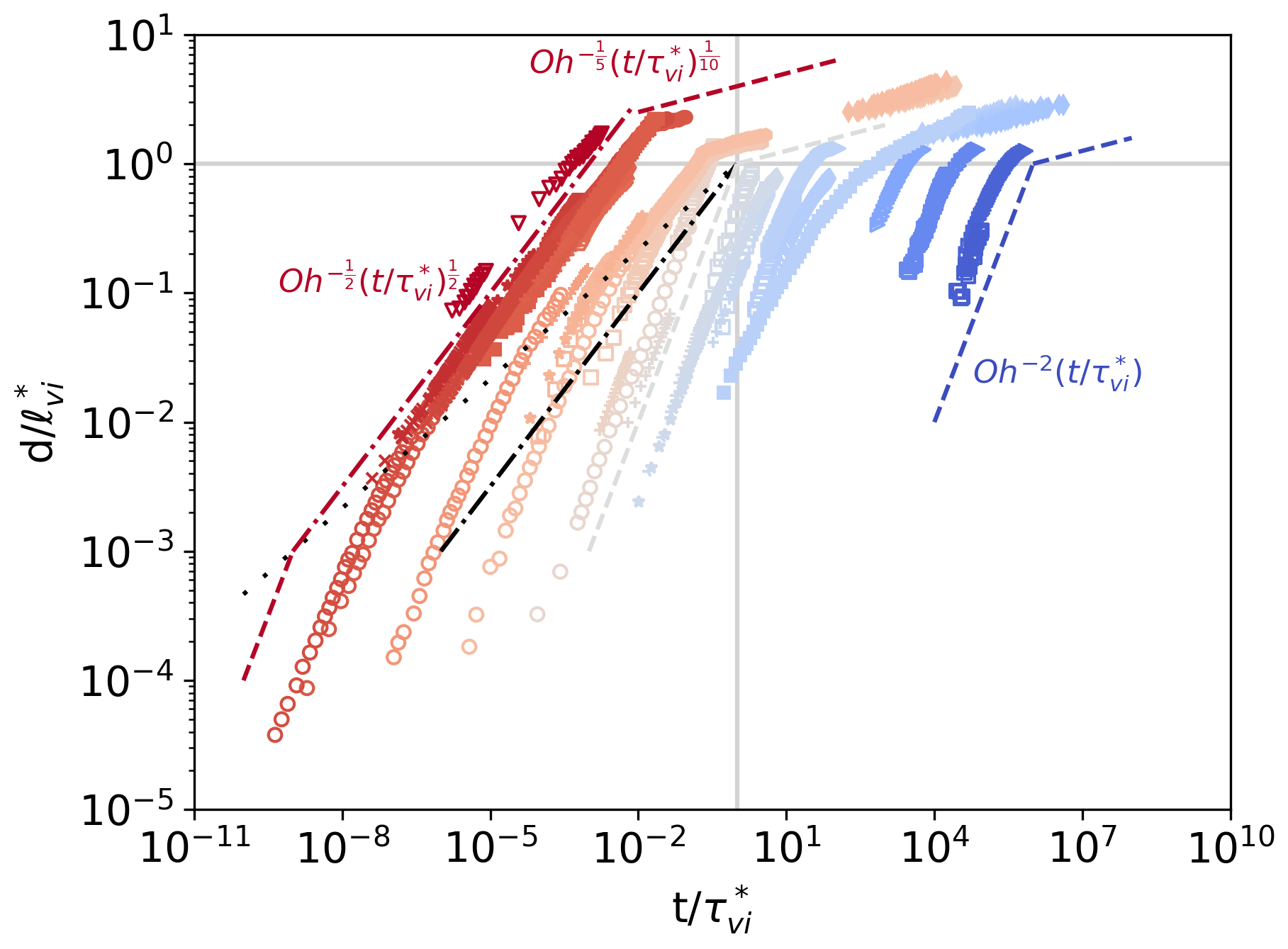
Figure 5: Spreading (filled symbols), coalescence (open symbols) and bubble pinching (crosses and stars) experiments for fluids with different degrees of inertia, viscosity and surface tension, represented in visco-inertial units. The dotted-dashed line gives the boundary layer scaling of Eq. 1. The color used for each data set gives to the value of the Ohnesorge number (full color scale in Fig. 6). The dashed lines give three examples of the purely visco-capillary scaling of Eq. 9 and Tanner’s regime of Eq. 11, for $\text{Oh}=10^{-3}$, 1 and $10^{3}$. The red dotted-dashed line gives Rayleigh’s regime of Eq. 20 for $\text{Oh}=10^{-3}$. The black loosely dotted line follows $d/\ell_{vi}^{*}=(t/\tau_{vi}^{*})^{\frac{1}{3}}$, which gives the loci of the intersections between the purely visco-capillary regime and Rayleigh’s regime. The black dotted dashed line is the boundary layer scaling $d/\ell_{vi}^{*}=(t/\tau_{vi}^{*})^{\frac{1}{2}}$. Details of the fluid properties for all data sets in the panels of this figure are given in ESI section 1^†. A schematic version of this plot is available in ESI-Fig. 1c^†. An animated version of this figures is provided in ESI^†.

V The Ohnesorge units

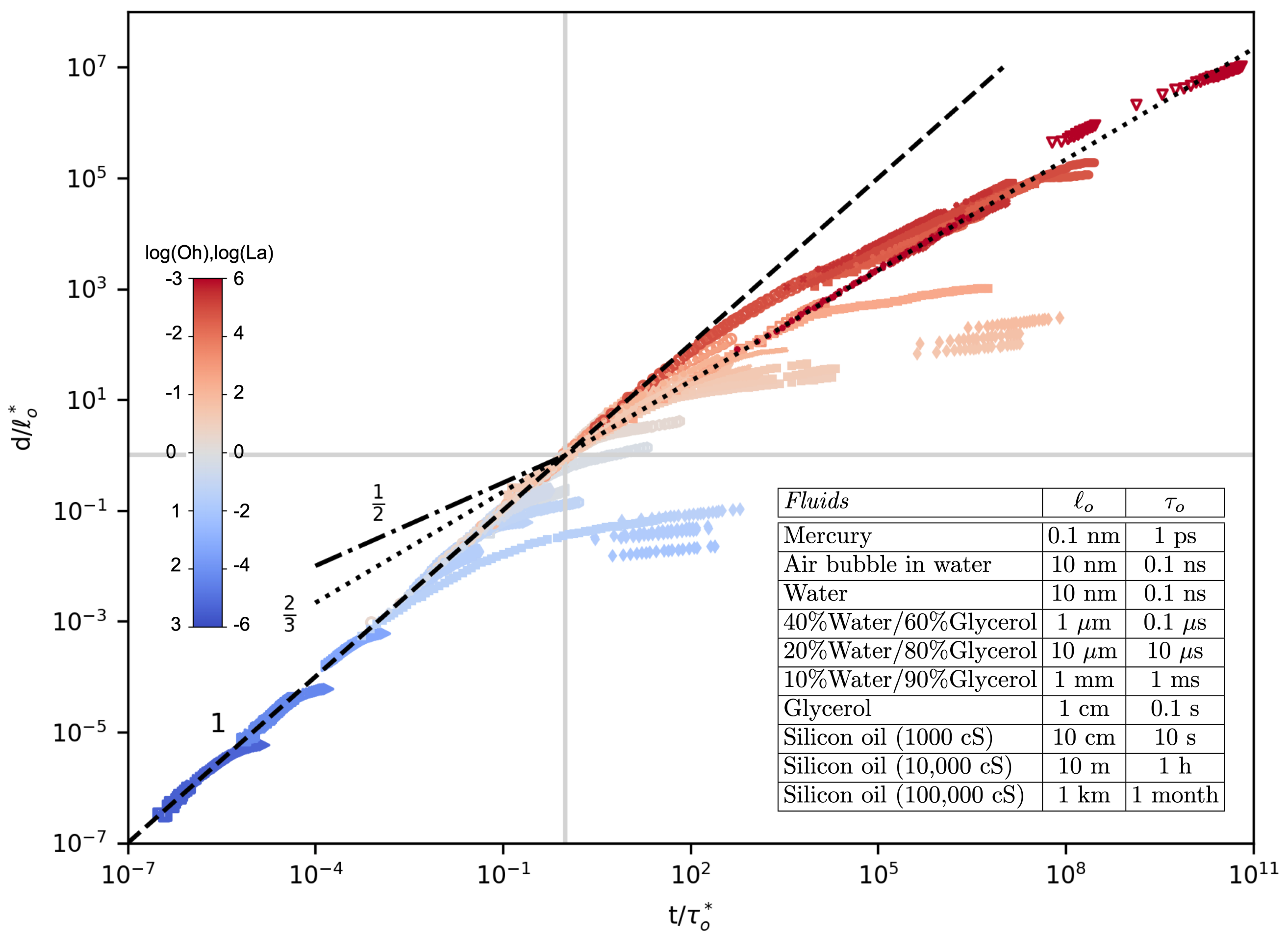
Figure 6: Spreading (filled symbols), coalescence (open symbols) and pinching (crosses and stars) experiments for fluids with different degrees of inertia, viscosity and surface tension, represented in Ohnesorge units. The color used for each data set gives to the value of the Ohnesorge or Laplace numbers. The few data sets with $\text{Oh}<10^{-3}$ are saturated and displayed with the color corresponding to $\text{Oh}=10^{-3}$. The inset table gives orders of magnitudes for $\ell_{o}$ and $\tau_{o}$ for a set of commonly used fluids (assuming normal temperature and pressure). Note that the dimensionless size and time include the dimensionless pre-factors, such that $\tau_{o}^{*}\equiv\gamma_{1}\tau_{o}$ and $\ell_{o}^{*}\equiv\gamma_{2}\ell_{o}$. The values of $\gamma_{1}$ and $\gamma_{2}$ for all curves are obtained from the pre-factors $\delta_{vc}$, $\delta_{Tan}$, $\delta_{ic}$ and $\delta_{Ray}$ (see ESI section 2E for details^†). Details of the fluid properties for all data sets in the panels of this figure are given in ESI section 1^†. Schematic and animated versions of this plot are also available in ESI^†.

So far, we have mentioned three systems of units: the visco-inertial units $\{\eta,\rho,D\}$, the visco-capillary units $\{\Gamma,\eta,D\}$ and the inertio-capillary units $\{\Gamma,\rho,D\}$. Using examples from boundary layers, spreading drops, coalescence and pinching we have illustrated the use of these units in association with three simple spreading laws, where ‘spreading’ is understood in a broad sense: $d\propto(\eta/\rho)^{\frac{1}{2}}t^{\frac{1}{2}}$, $d\propto(\Gamma/\eta)t$, and $d\propto(\Gamma/\rho)^{\frac{1}{3}}t^{\frac{2}{3}}$. These scaling laws are ‘simple’ in the sense that they can be obtained directly from dimensional analysis. These laws are also called ‘universal’ because they do not depend on any external parameter like the size of the drop $D$. One can verify that the visco-inertial regime corresponds to the only choice of exponent $\alpha$, such that $d/\ell_{vi}\propto(t/\tau_{vi})^{\alpha}$ does not depend on $D$. Similarly, the visco-capillary regime and the inertio-capillary regime correspond to the only exponents canceling the influence of $D$ in visco-capillary and inertio-capillary units respectively.

The three simple scalings intersect at the same spatio-temporal location:

$$\Big{(}\frac{\eta}{\rho}\Big{)}^{\frac{1}{2}}t^{\frac{1}{2}}=\frac{\Gamma}{\eta}t=\Big{(}\frac{\Gamma}{\rho}\Big{)}^{\frac{1}{3}}t^{\frac{2}{3}}\rightarrow t=\tau_{o}\quad\text{and}\quad d=\ell_{o}$$ (24)

The coordinates of the intersection between these three regimes are the time and lengthscale of a fourth system of units $\{\Gamma,\eta,\rho\}$, which we call the Ohnesorge units:

$$m_{o} \equiv\frac{\eta^{6}}{\Gamma^{3}\rho^{2}}$$ (25)

$$\ell_{o} \equiv\frac{\eta^{2}}{\Gamma\rho}$$ (26)

$$\tau_{o} \equiv\frac{\eta^{3}}{\Gamma^{2}\rho}$$ (27)

The Ohnesorge units have been invoked directly or indirectly in a number of studies, and date back to Haenlein, Weber and Ohnesorge, as stated in the introduction Haenlein (1931); Weber (1931); Ohnesorge (1936).

The magnitude of these units can vary widely depending on the properties of the fluid, as shown on a few examples in the inset of Fig. 6. A complete table with the values computed for all experiments used in this article is given in ESI^†. The Ohnesorge length and time vary from $\ell_{o}\simeq 3~{}\AA$ and $\tau_{o}\simeq 1$ ps for mercury Burton et al. (2004), and $\ell_{o}\simeq 1~{}$km and $\tau_{o}\simeq 4$ months for a viscous silicon oil Yao et al. (2005).

In Ohnesorge units, the scalings of the form $d/\ell_{o}\propto(t/\tau_{o})^{\alpha}$ admit three special values: for $\alpha=\frac{1}{2}$ the dynamics are independent of $\Gamma$ (Eq. 1), for $\alpha=1$ the dynamics are independent of $\rho$ (Eq. 9), and for $\alpha=\frac{2}{3}$ the dynamics are independent of $\eta$ (Eq. 15).

In contrast to the three systems introduced so far, the Ohnesorge units are purely intrinsic and do not depend on any extrinsic length $D$. Being at the crossroad of viscosity, inertia and surface tension, these units can be understood in a few different ways. For instance, the Ohnesorge time $\tau_{o}$ can be connected to the three other timescales by the Ohnesorge number as:

$$\tau_{vi}\xrightarrow{\times\text{Oh}}\tau_{ic}\xrightarrow{\times\text{Oh}}\tau_{vc}\xrightarrow{\times\text{Oh}^{2}}\tau_{o}$$ (28)

Thus, the two possible orderings for the four timescales are either $\tau_{vi}<\tau_{ic}<\tau_{vc}<\tau_{o}$ if Oh$>1$, or $\tau_{vi}>\tau_{ic}>\tau_{vc}>\tau_{o}$ if Oh$<1$. The Ohnesorge time can be understood as a visco-inertial time, or a visco-capillary time, or an inertio-capillary time when the distance $D$ is replaced by $\ell_{o}$.

The Ohnesorge length $\ell_{o}$ can be expressed as $\ell_{o}=\text{Oh}^{2}D$. Conversely, one can use the Ohnesorge length to define the Ohnesorge number as a ratio between intrinsic and extrinsic lengthscales, $\text{Oh}=(\ell_{o}/D)^{\frac{1}{2}}$. Alternatively, one can use the Laplace or Suratman number McKinley and Renardy (2011):

$$\text{La}\equiv\frac{D}{\ell_{o}}=\frac{1}{\text{Oh}^{2}}$$ (29)

Large values of the Laplace number correspond to more inertial dynamics, whereas small values correspond to more viscous ones. Note that the Ohnesorge number can also be expressed from the masses of the different systems of units, as $m_{o}=m_{vc}\text{Oh}^{4}=m_{ic}\text{Oh}^{6}$, where $m_{ic}=m_{vi}=\rho D^{3}$ is the actual mass (neglecting numerical factors).

In the Ohnesorge units, the characteristic stress is ${\Sigma}_{o}={m}_{o}.{\ell}_{o}^{-1}.{\tau}_{o}^{-2}=\Gamma^{2}\rho/\eta^{2}$. Again, this formula can be understood in a few ways. From an inertial perspective, one can write the stress as a dynamic pressure $\Sigma_{o}=\rho u_{o}^{2}$, where $u_{o}=\ell_{o}/\tau_{o}\propto\Gamma/\eta$ is the visco-capillary speed. From a viscous perspective, one can write the stress in a Newtonian way as $\Sigma_{o}=\eta(u_{o}/\ell_{o})$. From a capillary perspective, one can write the stress as a Laplace pressure, $\Sigma_{o}=\Gamma/\ell_{o}$. All these perspectives lead back to the same formula.

The Ohnesorge units are ideal to represent spreading, coalescence and pinching dynamics from a purely intrinsic perspective. All data reproduced in this article are shown in Ohnesorge units in Fig. 6. These intrinsic units allow to circumvent the challenges faced with the overlap of data sets in Fig. 4 and 5, where the purely inertio-capillary data had to be plotted separately. Here, all data can be shown simultaneously, including 71 separate curves $d(t)$ obtained from 25 different studies Cazabat and Stuart (1986); Biance et al. (2004); Eddi et al. (2013); Chen and Bonaccurso (2014); Menchaca-Rocha et al. (2001); Wu et al. (2004); Yao et al. (2005); Thoroddsen et al. (2005, 2005); Aarts et al. (2005); Aarts and Lekkerkerker (2008); Yokota and Okumura (2011); Paulsen et al. (2011, 2014); Soto et al. (2018); Rahman et al. (2019); Chen and Steen (1997); McKinley and Tripathi (2000); Chen et al. (2002); Burton et al. (2004, 2005, 2007); Keim et al. (2006); Bolanos-Jiménez et al. (2009); Goldstein et al. (2010), spanning 7 orders of magnitude in the value of Oh, and respectively 14 and 18 orders of magnitude in the values of $d/\ell_{o}$ and $t/\tau_{o}$. In this representation, the different values of extrinsic length $D$ emerge as different points of departure from comparatively more universal trends.

For $\text{Oh}>1$, i.e. $\text{La}<1$, the data seem to converge on the linear scaling when $d/\ell_{o}\ll\text{La}$, i.e. when $\Lambda\ll 1$. If $\Lambda\gtrsim 1$, different departures are possible depending on the boundary conditions. For instance, for total wetting, spreading data can follow Tanner’s law $d/\ell_{o}\propto\text{Oh}^{-\frac{9}{5}}(t/\tau_{o})^{\frac{1}{10}}$.

For $\text{Oh}<1$, i.e. $\text{La}>1$, the asymptotic departures similarly correspond to different values of the extrinsic size $D$. Whereas the linear scaling seems quite attractive to all dynamics for $d/\ell_{o}\ll\text{La}<1$, multiple trends are possible for $d/\ell_{o}\ll\text{La}>1$. For instance, spreading, coalescence and bubble pinching can remain on the linear scaling as long as $d/\ell_{o}<\text{Oh}^{-1}$, then follow the size-dependent inertio-capillary regime, now written as $d/\ell_{o}\propto\text{Oh}^{-\frac{1}{2}}(t/\tau_{o})^{\frac{1}{2}}$. This intermediate regime reaches $d\propto D$ when crossing the $\frac{2}{3}$ trend. Not all data follow this path through the size-dependent inertio-capillary regime. In particular, we have seen that the pinching dynamics of liquids can transition from a purely visco-capillary regime to a purely inertio-capillary $\frac{2}{3}$ regime, as soon as $d>\ell_{o}$. A zoom on the quadrant $d>\ell_{o}$ and $t>\tau_{o}$ of Fig. 6 is provided in ESI-Fig. 11^†, to allow for easier distinction between the different possible paths.

What are the conditions dynamics must meet to exhibit an intermediate size-dependent inertio-capillary $\frac{1}{2}$ regime instead of directly following the purely inertio-capillary $\frac{2}{3}$ regime? For instance, bubbles of air in water will exhibit the $\frac{1}{2}$ regime, whereas water drops will exhibit the $\frac{2}{3}$ regime Eggers and Villermaux (2008). For spreading drops, results from Biance et al. and Chen et al. corresponding to $\text{Oh}\simeq 10^{-1}-10^{-3}$ exhibit the $\frac{1}{2}$ scaling Biance et al. (2004); Chen and Bonaccurso (2014). However, we notice that data from Eddi et al. Eddi et al. (2013) for $\text{Oh}\simeq 10^{-1}-1$ can be seen to follow the $\frac{2}{3}$ regime (see ESI-Fig. 11 for details^†). The conditions bringing dynamics along the $\frac{1}{2}$ or $\frac{2}{3}$ regimes remain unclear, but may be related to the initial shape of the drop Courbin et al. (2009); Eddi et al. (2013). Moreover, some dynamics even seem to follow the $\frac{1}{2}$ or $\frac{2}{3}$ scaling for $d<\ell_{o}$. These data are not shown in Fig. 6, but are given in ESI-Fig. 12^†. The coexistence of different parallel regimes was manifested in Fig. 3 for $\text{Oh}<1$, and dimensional analysis alone does not preclude the existence of multiples regimes for $\text{Oh}>1$. For instance, if the boundary layer dynamics are interpreted as having $\text{Oh}=1$, then $\ell_{o}=D$, and the data follow the $\frac{1}{2}$ scaling drawn with the dotted-dashed line in Fig. 6. More surprising, the data on spreading drops from Eddi et al. Eddi et al. (2013), with $\text{Oh}\gtrsim 1$ are quite close from the $\frac{2}{3}$ scaling drawn as a dotted line in Fig. 6, depending on the pre-factors $\gamma_{1}$ and $\gamma_{2}$ that one may choose (see ESI-Fig. 12 for details^†). Note also that in the context of the coalescence of drops with $\text{Oh}\propto 1$, a regime combining inertial, viscosity and surface tension has been evidenced Paulsen et al. (2012).

In reviewing the literature on spreading, pinching, and coalescence, we thought that spreading and coalescence would show a stronger dependency on geometry and display the size-dependent $\frac{1}{2}$ regime for $\text{Oh}<1$, whereas pinching would follow the more universal $\frac{2}{3}$ regime. Experiments seem to paint a more nuanced picture.

VI Departures from Ohnesorge’s units

All data discussed in this article abide quite well to the Ohnesorge units. Despite the fact that the data cover an unprecedentedly large spectrum, they only represent a small fraction of the possible dynamics influenced by viscosity, density and surface tension. For future studies to include more data, we see two complementary avenues set by answering the following questions: what kind of additional data would fit within the Ohnesorge units, and what kind would not?

First, one may wonder about dynamics abiding to Ohnesorge units but in non-trivial ways. For instance, in the context of the spreading of liquid-on-liquid, one may encounter scalings of the form $d/\ell_{o}\propto(t/\tau_{o})^{\alpha}$, with $\alpha$ different from 1, $\frac{1}{2}$ or $\frac{2}{3}$. In particular, $\alpha=\frac{3}{4}$ has been described in several instances Wang et al. (2015); Berg (2009). Such non-trivial regime in Ohnesorge units is analogous to Tanner’s law or to Rayleigh’s law, in the sense that it cannot be derived directly from dimensional analysis.

For the data represented in Fig. 6, departures from the three simple scalings ($1$, $\frac{1}{2}$ and $\frac{2}{3}$) are all associated with the existence of an extrinsic or ‘integral’ lengthscale $D$. In all experiments considered here, the spreading, coalescence or pinching dynamics are ‘free’, in the sense that they happen spontaneously, without any imposed speed $U$ or acceleration $G$. If non-negligible extrinsic speed or acceleration are present, the ‘integral scale’ is not solely characterized by a size $D$. Hence, in these ‘forced’ cases of spreading, coalescence or pinching, one would expect the departures from Ohnesorge’s units to be more varied. Already in Fig. 2c we noticed that gravity, i.e. an acceleration $G=g$ can alter Tanner’s law at long time, leading to $d\sim t^{\frac{1}{8}}$ instead of $d\sim t^{\frac{1}{10}}$ Cazabat and Stuart (1986). Similarly, an extrinsic speed can have a very significant impact, as was indeed demonstrated for jetting by Ohnesorge himself Ohnesorge (1936).

Departures from the Ohnesorge units can also be due to additional intrinsic mechanisms beyond viscosity, inertia and capillarity. For instance, in the case of viscoelastic fluids an elasticity $\Sigma$ becomes relevant and generate an intrinsic ‘relaxation time’ $\tau_{ve}=\eta/\Sigma$, which can lead to exponential regimes, so far mostly described in the context of pinching McKinley (2005); Dinic and Sharma (2019, 2020).

In general if the departure from Ohnesorge units can be traced back to a quantity $Q$, then a dimensionless number $N=Q/Q_{o}$ can be built, where $Q_{o}$ has the same dimensions than $Q$ and is given in Ohnesorge units. For instance, if $Q=D$, then $N=D/\ell_{o}=\text{La}=\text{Oh}^{-2}$. If $Q=G$, then $N=G/G_{o}=G\eta^{4}/\Gamma^{3}\rho=\text{Bo}\text{Oh}^{4}$, where $\text{Bo}=\rho GD^{2}/\Gamma$ is the Bond number De Gennes et al. (2013). If $Q=\Sigma$, then $N=\Sigma/\Sigma_{o}=\Sigma\eta^{2}/\Gamma^{2}\rho=\text{Ec}^{-1}\text{Oh}^{2}$, where $\text{Ec}=\Gamma/\Sigma D$ is the elasto-capillary number McKinley (2005).

Another way in which dynamics can differ from those depicted in Fig. 6 is in the presence of competing choices of densities, viscosities or surface tensions. In this article, we focused on cases where a single choice of material parameters was possible, but it is not necessarily the case. In general, ratios of the material properties of the inner and outer fluids can have an impact on the dynamics. This issue has been investigated for spreading Bazazi et al. (2018); Jose and Cubaud (2017), coalescence Paulsen et al. (2014); Jose and Cubaud (2017) and pinching Verbeke et al. (2020) and we hope to be able to include these studies in the future. Some of these dynamics may fit well with the Ohnesorge units with minimal adjustments. For instance, the coalescence of bubbles in a viscous fluid can give rise to a scaling $d/\ell_{vc}\propto(t/\tau_{vc})^{\frac{1}{2}}$, when the outer viscosity is used to compute the visco-capillary time $\tau_{vc}$ Paulsen et al. (2014).

VII Conclusion

Because lengths, durations and masses are so engraved in our understanding of physical reality, we tend to forget that their fundamental stature is somewhat of a convention. International standards encourage the use of units based on the dimensions of mass, length and time, reminding for example that a viscosity of 1 poise stands for 0.1 kg.m^-1.s^-1. This approach to physical quantities like viscosity, density or surface tension is rooted in metrology. For instance, if one needs to measure viscosity, one will have to rely on some associated measurements of size (e.g. dimensions of the rheometer), time (e.g. in measuring speeds) and mass (e.g. if stress is measured through a torque, itself measured by a mass and pulley system). In everyday life, distances, durations and to some extent masses are the most easily available measures of the physical world. However, the microcosm unfolding at the scale of drops of fluid, spreading, pinching and coalescing, is quite different from ours. There, space, time and mass are derived quantities, produced by the interplay of three basic dimensions called viscosity, surface tension and density. By elevating these three quantities as fundamental dimensions, recent studies have greatly advanced our understanding of capillary phenomena. Building on years of experimental studies on spreading, pinching and coalescence, they have shown how the different classes of behaviors are quantitatively related by the use of appropriate units based on $\eta$, $\Gamma$ and $\rho$.

The three simple spreading laws discussed in this article (Eq. 1, 9 and 15) provide the three essential ways in which space-time emerges in the universe of droplets, the three ways in which length and duration are coupled. One way to interpret the Ohnesorge units is as giving the dimensions of length, time and mass as derived from those of viscosity, surface tension and density. For instance, $[t]=[\eta]^{3}.[\Gamma]^{-2}.[\rho]^{-1}$. This equation on the dimensions is always true, even beyond drops of fluids. What is most striking is that if the equation is used without the brackets, i.e. to yield numerical values, then the derived timescale turns out to be very significant to the dynamics in the world of drops. As shown in Fig. 6, the Ohnesorge time $\tau_{o}$ is at the crossroads of an array of different phenomena and often marks the turning point between distinct dynamical regimes.

The Ohnesorge units formalize the essential intrinsic properties of a world governed by viscosity, surface tension and density. However, this universe is not unbounded, and its limit overlaps with our more familiar realm through the influence of the ‘integral’ or ‘extrinsic’ length $D$. In this article, we have carefully shown how the intrinsic Ohnesorge units can be transformed by the addition of the length $D$, and how size-dependent dynamical regimes like those of Tanner or Rayleigh can become preponderant. Together, the four systems of units described in this article provide the four ways to choose three parameters from the set $\{\Gamma,\eta,\rho,D\}$. These four parameters are connected to each other by the Ohnesorge number, which provides a natural way to distinguish between ‘more viscous’ ($\text{Oh}>1$) and ‘more inertial’ ($\text{Oh}<1$) dynamics.

Conflicts of interest

There are no conflicts to declare.

References

- Ohnesorge (1936) W. V. Ohnesorge, ZAMM-Journal of Applied Mathematics and Mechanics/Zeitschrift für Angewandte Mathematik und Mechanik, 1936, 16, 355–358.
- Eggers (1997) J. Eggers, Reviews of Modern Physics, 1997, 69, 865.
- Basaran (2002) O. A. Basaran, AIChE Journal, 2002, 48, 1842.
- McKinley and Renardy (2011) G. H. McKinley and M. Renardy, Physics of Fluids, 2011, 23, 127101.
- Rayleigh et al. (1879) L. Rayleigh et al., Proc. R. Soc. London, 1879, 29, 71–97.
- Haenlein (1931) A. Haenlein, Forschung auf dem Gebiet des Ingenieurwesens, 1931, 2, 139–149.
- Weber (1931) C. Weber, Z. Angew. Math. Mech., 1931, 2, 136.
- Leger and Joanny (1992) L. Leger and J. Joanny, Reports on Progress in Physics, 1992, 55, 431.
- Stone (1994) H. A. Stone, Annual Review of Fluid Mechanics, 1994, 26, 65–102.
- Middleman (1995) S. Middleman, Modeling axisymmetric flows: dynamics of films, jets, and drops, Academic Press, 1995.
- Oron et al. (1997) A. Oron, S. H. Davis and S. G. Bankoff, Reviews of Modern Physics, 1997, 69, 931.
- McKinley (2005) G. H. McKinley, Rheology Reviews, 2005, 1, .
- Yarin (2006) A. L. Yarin, Annual Review of Fluid Mechanics, 2006, 38, 159–192.
- Leal (2007) L. G. Leal, Advanced transport phenomena: fluid mechanics and convective transport processes, Cambridge University Press, 2007, vol. 7.
- Villermaux (2007) E. Villermaux, Annual Review of Fluid Mechanics, 2007, 39, 419–446.
- Eggers and Villermaux (2008) J. Eggers and E. Villermaux, Reports on progress in physics, 2008, 71, 036601.
- Bonn et al. (2009) D. Bonn, J. Eggers, J. Indekeu, J. Meunier and E. Rolley, Reviews of modern physics, 2009, 81, 739.
- De Gennes et al. (2013) P.-G. De Gennes, F. Brochard-Wyart and D. Quéré, Capillarity and wetting phenomena: drops, bubbles, pearls, waves, Springer Science & Business Media, 2013.
- Snoeijer and Andreotti (2013) J. H. Snoeijer and B. Andreotti, Annual review of fluid mechanics, 2013, 45, 269–292.
- Eggers and Fontelos (2015) J. Eggers and M. A. Fontelos, Singularities: formation, structure, and propagation, Cambridge University Press, 2015, vol. 53.
- Kavehpour (2015) H. P. Kavehpour, Annual Review of Fluid Mechanics, 2015, 47, 245–268.
- Barenblatt (2003) G. I. Barenblatt, Scaling, Cambridge University Press, 2003, vol. 34.
- Castrejón-Pita et al. (2015) J. R. Castrejón-Pita, A. A. Castrejón-Pita, S. S. Thete, K. Sambath, I. M. Hutchings, J. Hinch, J. R. Lister and O. A. Basaran, Proceedings of the National Academy of Sciences, 2015, 112, 4582–4587.
- Dinic and Sharma (2019) J. Dinic and V. Sharma, Proceedings of the National Academy of Sciences, 2019, 116, 8766–8774.
- Dinic and Sharma (2020) J. Dinic and V. Sharma, Macromolecules, 2020, 53, 3424–3437.
- Landau and Lifshitz (1959) L. Landau and E. Lifshitz, Fluid Mechanics, Pergamon, 1959, vol. 61.
- Blasius (1907) H. Blasius, Grenzschichten in Flüssigkeiten mit kleiner Reibung, Druck von BG Teubner, 1907.
- Schlichting and Gersten (2016) H. Schlichting and K. Gersten, Boundary-layer theory, Springer, 2016.
- Paulsen et al. (2011) J. D. Paulsen, J. C. Burton and S. R. Nagel, Physical Review Letters, 2011, 106, 114501.
- Aarts et al. (2005) D. G. Aarts, H. N. Lekkerkerker, H. Guo, G. H. Wegdam and D. Bonn, Physical Review Letters, 2005, 95, 164503.
- Aarts and Lekkerkerker (2008) D. G. Aarts and H. N. Lekkerkerker, Journal of Fluid Mechanics, 2008, 606, 275–294.
- Rahman et al. (2019) M. M. Rahman, W. Lee, A. Iyer and S. J. Williams, Physics of Fluids, 2019, 31, 012104.
- Yao et al. (2005) W. Yao, H. Maris, P. Pennington and G. Seidel, Physical Review E, 2005, 71, 016309.
- Eddi et al. (2013) A. Eddi, K. G. Winkels and J. H. Snoeijer, Physics of Fluids, 2013, 25, 013102.
- Cazabat and Stuart (1986) A. Cazabat and M. C. Stuart, The Journal of Physical Chemistry, 1986, 90, 5845–5849.
- Yokota and Okumura (2011) M. Yokota and K. Okumura, Proceedings of the National Academy of Sciences, 2011, 108, 6395–6398.
- Tanner (1979) L. Tanner, Journal of Physics D: Applied Physics, 1979, 12, 1473.
- Eggers et al. (1999) J. Eggers, J. R. Lister and H. A. Stone, Journal of Fluid Mechanics, 1999, 401, 293–310.
- Hopper (1990) R. W. Hopper, Journal of Fluid Mechanics, 1990, 213, 349–375.
- Bolanos-Jiménez et al. (2009) R. Bolanos-Jiménez, A. Sevilla, C. Martínez-Bazán, D. Van Der Meer and J. Gordillo, Physics of Fluids, 2009, 21, 072103.
- Burton et al. (2007) J. Burton, J. Rutledge and P. Taborek, Physical Review E, 2007, 75, 036311.
- Chen and Steen (1997) Y.-J. Chen and P. Steen, Journal of Fluid Mechanics, 1997, 341, 245–267.
- Chen et al. (2002) A. U. Chen, P. K. Notz and O. A. Basaran, Physical Review Letters, 2002, 88, 174501.
- Goldstein et al. (2010) R. E. Goldstein, H. K. Moffatt, A. I. Pesci and R. L. Ricca, Proceedings of the National Academy of Sciences, 2010, 107, 21979–21984.
- Burton et al. (2004) J. Burton, J. Rutledge and P. Taborek, Physical Review Letters, 2004, 92, 244505.
- Biance et al. (2004) A.-L. Biance, C. Clanet and D. Quéré, Physical Review E, 2004, 69, 016301.
- Chen and Bonaccurso (2014) L. Chen and E. Bonaccurso, Physical Review E, 2014, 90, 022401.
- Menchaca-Rocha et al. (2001) A. Menchaca-Rocha, A. Martínez-Dávalos, R. Nunez, S. Popinet and S. Zaleski, Physical Review E, 2001, 63, 046309.
- Thoroddsen et al. (2005) S. Thoroddsen, K. Takehara and T. Etoh, Journal of Fluid Mechanics, 2005, 527, 85–114.
- Thoroddsen et al. (2005) S. Thoroddsen, T. Etoh, K. Takehara and N. Ootsuka, Physics of Fluids, 2005, 17, 071703.
- Paulsen et al. (2014) J. D. Paulsen, R. Carmigniani, A. Kannan, J. C. Burton and S. R. Nagel, Nature communications, 2014, 5, 1–7.
- Soto et al. (2018) Á. M. Soto, T. Maddalena, A. Fraters, D. Van Der Meer and D. Lohse, Journal of Fluid Mechanics, 2018, 846, 143–165.
- Burton et al. (2005) J. Burton, R. Waldrep and P. Taborek, Physical Review Letters, 2005, 94, 184502.
- Keim et al. (2006) N. C. Keim, P. Møller, W. W. Zhang and S. R. Nagel, Physical Review Letters, 2006, 97, 144503.
- Keller and Miksis (1983) J. B. Keller and M. J. Miksis, SIAM Journal on Applied Mathematics, 1983, 43, 268–277.
- Day et al. (1998) R. F. Day, E. J. Hinch and J. R. Lister, Physical Review Letters, 1998, 80, 704.
- Deblais et al. (2018) A. Deblais, M. Herrada, I. Hauner, K. P. Velikov, T. Van Roon, H. Kellay, J. Eggers and D. Bonn, Physical Review Letters, 2018, 121, 254501.
- Dinic and Sharma (2019) J. Dinic and V. Sharma, Physics of Fluids, 2019, 31, 021211.
- Eggers et al. (2007) J. Eggers, M. Fontelos, D. Leppinen and J. Snoeijer, Physical Review Letters, 2007, 98, 094502.
- Courbin et al. (2009) L. Courbin, J. C. Bird, M. Reyssat and H. Stone, Journal of Physics: Condensed Matter, 2009, 21, 464127.
- Carlson et al. (2012) A. Carlson, G. Bellani and G. Amberg, Physical Review E, 2012, 85, 045302.
- Israelachvili (2015) J. N. Israelachvili, Intermolecular and surface forces, Academic press, 2015.
- Wu et al. (2004) M. Wu, T. Cubaud and C.-M. Ho, Physics of Fluids, 2004, 16, L51–L54.
- McKinley and Tripathi (2000) G. H. McKinley and A. Tripathi, Journal of Rheology, 2000, 44, 653–670.
- Eddi et al. (2013) A. Eddi, K. Winkels and J. Snoeijer, Physical Review Letters, 2013, 111, 144502.
- Paulsen et al. (2012) J. D. Paulsen, J. C. Burton, S. R. Nagel, S. Appathurai, M. T. Harris and O. A. Basaran, Proceedings of the National Academy of Sciences, 2012, 109, 6857–6861.
- Wang et al. (2015) X. Wang, E. Bonaccurso, J. Venzmer and S. Garoff, Colloids and Surfaces A: Physicochemical and Engineering Aspects, 2015, 486, 53–59.
- Berg (2009) S. Berg, Physics of Fluids, 2009, 21, 032105.
- Bazazi et al. (2018) P. Bazazi, A. Sanati-Nezhad and S. Hejazi, Physical Review E, 2018, 97, 063104.
- Jose and Cubaud (2017) B. M. Jose and T. Cubaud, Physical Review Fluids, 2017, 2, 111601.
- Verbeke et al. (2020) K. Verbeke, S. Formenti, F. B. Vangosa, C. Mitrias, N. K. Reddy, P. D. Anderson and C. Clasen, Physical Review Fluids, 2020, 5, 051901.