Optimal Rate Adaption in Federated Learning with Compressed Communications

Abstract

Federated Learning (FL) incurs high communication overhead, which can be greatly alleviated by compression for model updates. Yet the tradeoff between compression and model accuracy in the networked environment remains unclear and, for simplicity, most implementations adopt a fixed compression rate only. In this paper, we for the first time systematically examine this tradeoff, identifying the influence of the compression error on the final model accuracy with respect to the learning rate. Specifically, we factor the compression error of each global iteration into the convergence rate analysis under both strongly convex and non-convex loss functions. We then present an adaptation framework to maximize the final model accuracy by strategically adjusting the compression rate in each iteration. We have discussed the key implementation issues of our framework in practical networks with representative compression algorithms. Experiments over the popular MNIST and CIFAR-10 datasets confirm that our solution effectively reduces network traffic yet maintains high model accuracy in FL.

I Introduction

In today’s networked world, data are generated and stored everywhere [1]. While conventional learning tools are mostly centralized, relying on cloud datacenters to aggregate and analyze the data, Federated Learning (FL) has been built distributed [2], allowing clients physically remote from each other to collaboratively train learning models over the Internet. It effectively utilizes the rich data spread across different geo-locations and organizations, without compromising their privacy  [3], e.g., for smart devices to predict human trajectories [4] or for healthcare systems to develop predictive models [5].

To coordinate the participating clients, a parameter server (PS) has to be deployed in a FL system for collecting, aggregating and distributing model updates, often in many iterations. This inevitably incurs huge communication overhead, which severely slows down the training process or even makes FL impractical if the model is of high dimensions [6]. To address this challenge, compression algorithms have been employed by FL clients [7], which use quantization or sparsification to reduce the size of a model update. For instance, TernGrad [8] quantifies each model update to one of three centroid values in an unbiased manner. This can speed up the training of AlexNet on 8 GPUs by 3.4 times. Assuming that each original model update takes 4 bytes; indexing model updates into four centroids will only need 2 bits, or only $6.25\%$ of the original traffic for each update from the client to the PS [7].

While model compression accelerates computing and communication, it potentially reduces the final model accuracy [9]. For simplicity, most of the existing compression algorithms have fixed their compression rates [7], which can limit their applicability and effectiveness. There have been significant studies on the convergence analysis of FL [10, 11]. The impact of model compression however has yet to be explored, not to mention the optimal rate configuration with compression.

In this paper, we for the first time systematically examine the tradeoff between the compression rate and model accuracy for FL in the networked environment. We show that the influence of the compression error on the final model accuracy is closely related to the learning rate. Specifically, we factor the compression error of each global iteration into the convergence rate analysis given both strongly convex and non-convex loss functions. We then present an adaptation framework to maximize the final model accuracy by strategically adjusting the compression rate in each global iteration. Our solution works well for dynamic networks and is generally applicable to different unbiased compression algorithms. We have discussed the key implementation issues of our framework in practical networks, with case studies of two representative compression algorithms, namely, PQ [12] and QSGD [13]. Experiments over the popular MNIST and CIFAR-10 datasets [14] confirm that our framework can effectively improve the final model accuracy of FL under the same network bandwidth constraints for both IID and non-IID sample distributions.

The rest of the paper is organized as below. State-of-the-art relevant works are discussed in Sec. II. Preliminary knowledge regarding model average algorithms and compression algorithms are introduced in Sec. III. We then present the convergence rate analysis in Sec. IV, together with the rate-optimized adaptive compression framework in Sec. V. We discuss the experiment results in Sec. VI and conclude the paper in Sec. VII.

II Related Works

In this section, we discuss related works in Federated Learning (FL) from two aspects, namely, model averaging and model compression. The former is the foundation for FL, and the later is essential for minimizing traffic overhead in FL.

II-A FL Model Averaging

In Federated Learning (FL) [15, 16], decentralized clients collaboratively train machine learning models via model averaging, i.e., iteratively averaging locally trained models towards global optimum [2]. It runs Stochastic Gradient Descent (SGD) in parallel on a subset of devices and then averages the resulting model updates via a central server once in a while. The convergence rates of FedAvg have been analyzed in [10] with strongly convex loss functions and [11] with non-convex loss functions, respectively. There have also been variants of FedAvg that target different application scenarios. Wang et al. in [17] designed a control algorithm to balance local updates and global aggregation in FL under limited resource in edge computing; FEDL [18] optimizes the allocation of resources in wireless networks to balance the convergence and resource consumption. Our work focuses on the classical FedAvg with model compression; yet our solution can be generalized to work with these extended versions.

II-B FL Model Compression

Transmitting model updates in a large scale network incurs heavy traffic overhead. The original FedAvg [2] increases the number of local iterations on clients to minimize the costly global communications. Parallel FL architecture [19] seeks to reduce the network bandwidth consumption through using multiple servers. Our work however focuses on model compression [20, 21], which is orthogonal to them, and can work together with them to maximize traffic reduction.

Model compression in FL can be achieved through two methods [22], namely, sparsification and quantization.

Sparsification algorithms select only a small number of significant model updates for transmission. The DGC algorithm proposed in [23] discards 99.9% of gradients in communication, achieving a very high compression rate. Gaia [24] dynamically eliminates insignificant communications, and STC [9] compresses uploaded and downloaded data simultaneously through sparse and ternary methods. DC2 [25] further explores the delay-traffic trade off through adaptively coupling compression control and network latency. Although sparsification can be quite effective, the solutions above are mostly biased, implying that they may not guarantee the convergence of FL and hence is not our focus in this work.

Quantization algorithms map model updates to a small set of discrete values. For instance, the QSGD algorithm [13] generates a random number based on each model update and map each update to a centroid. The PQ algorithm [12] splits model updates into intervals with a number of centroids, and each model update is randomly quantified to a centroid in an unbiased manner. In [8], Wen et al. optimized communication by quantizing model updates to ternary values. The mapping in most quantization algorithms is unbiased. Yet most of them adopt a fixed compression rate because the relation between the compression error and the learning rate is largely unknown. In this paper, we for the first time analyze the effect of the compression on the model convergence for both strongly convex and non-convex cases. We accordingly propose an adaptive compression framework with optimal rate allocation, which seeks the balance between model accuracy and communication overhead for FL over real world networks.

III Background and System Model

In this section, we introduce the necessary background on Federated Learning, particularly on the model averaging algorithm, i.e., FedAvg [2], and the compression algorithms. We also outline our system model with adaptive compression and summarize the key notations.

III-A Federated Learning Basics

In FL, data samples are distributed on $N$ clients, where the data set owned by client $i$ is $\mathcal{D}_{i}$. All $N$ clients collaboratively train a machine learning model, and their local results are aggregated through model averaging, typical through FedAvg or its variants [26]. A loss function of the training model on client $i$ can be denoted by:

$$F_{i}(\mathbf{w},\mathcal{D}_{i})=\frac{1}{|\mathcal{D}_{i}|}\sum_{\forall\xi\in\mathcal{D}_{i}}f(\mathbf{w},\xi).$$ (1)

Here, $\mathbf{w}\in\mathbb{R}^{d}$ with dimension $d$ is the model parameters to be learned, $|\mathcal{D}_{i}|$ denotes the size of client $i$’s dataset, and $f(\mathbf{w},\xi)$ denotes the loss function calculated by a specific sample $\xi$. The goal of FL is to train the model parameters such that the global loss function can be minimized, that is

$$\min_{\mathbf{w}}\quad F(\mathbf{w})=\sum_{i=1}^{N}p_{i}F_{i}(\mathbf{w},\mathcal{D}_{i}),$$ (2)

where $p_{i}$ represents the weight of client $i$, which is typically set to $p_{i}=\frac{|\mathcal{D}_{i}|}{\sum_{i^{\prime}=1}^{N}|\mathcal{D}_{i^{\prime}}|}$.

FedAvg conducts multiple global iterations to iteratively reduce the global loss function $F(\mathbf{w})$. In global iteration $t$, a Parameter Server (PS) randomly selects $K$ clients, denoted by $\mathcal{K}_{t}$, to participate in model training. Each selected client downloads the latest model parameters denoted by $\mathbf{w}_{t}$ from the PS, and then conducts $E$-round local iterations with the local data samples. Each round works as follows:

$$\mathbf{w}^{i}_{t,j+1}=\mathbf{w}^{i}_{t,j}-\eta_{t}\nabla F_{i}(\mathbf{w}^{i}_{t,j},\mathcal{B}^{i}_{t,j}),$$ (3)

where $j$ represents the $j^{th}$ local iteration, $\eta_{t}$ represents the learning rate at global iteration $t$, and $\mathcal{B}^{i}_{t,j}$ represents the sample batch with size $B$ randomly selected by client $i$ for this local iteration. After the $E$ local iterations, participating clients will send model updates $\mathbf{U}^{i}_{t}=\sum_{j=0}^{E-1}\nabla F_{i}(\mathbf{w}^{i}_{t,j},\mathcal{B}^{i}_{t,j})$ back to the PS for aggregation, as follows

$$\mathbf{w}_{t+1}=\mathbf{w}_{t}\!\!-\!\!\eta_{t}\sum_{i\in\mathcal{K}_{t}}\frac{|\mathcal{D}_{i}|}{\sum_{i^{{}^{\prime}}\in\mathcal{K}_{t}}|\mathcal{D}_{i^{{}^{\prime}}}|}\mathbf{U}^{i}_{t}.$$ (4)

III-B Compression with Rate Adaptation

Uploading model updates $\mathbf{U}^{i}_{t}$ to the PS can be very time consuming in dynamic network environment given the limited upload bandwidth [7]. Compression can be applied to $\mathbf{U}^{i}_{t}$, so as to reduce the traffic. As mentioned in the previous section, we focus on quantization-based compression, which uses a small number of centroids to represent model updates. Let $\widetilde{\mathbf{U}}^{i}_{t}$ denote the compression of $\mathbf{U}^{i}_{t}$. To avoid compromising the convergence rate of FL, $\widetilde{\mathbf{U}}^{i}_{t}$ is typically set as a random variable with expectation $\mathbb{E}\widetilde{\mathbf{U}}^{i}_{t}=\mathbf{U}^{i}_{t}$ [13]. In other words, $\widetilde{\mathbf{U}}^{i}_{t}$ is the unbiased estimation of $\mathbf{U}^{i}_{t}$. Let $\widetilde{\mathbf{U}}^{i}_{t}$ be a discrete random variable with only $Z$ possible values, denoted by $u_{1},u_{2},\dots,u_{Z}$, which are referred to as $Z$ centroids for compression.

Figure 1 outlines the process to transmit model updates from a particular client to the PS with a fixed compression rate and adaptive compression rates, respectively. Though the former, for its simplicity, has been adopted in most existing works on quantization, our analysis in the next section suggests that the compression rate should be adjusted according to the influence of the compression error in each communication round in a real world network environment with resource constraints and dynamics, and we accordingly develop the optimal adaption strategy that maximizes the final model accuracy.

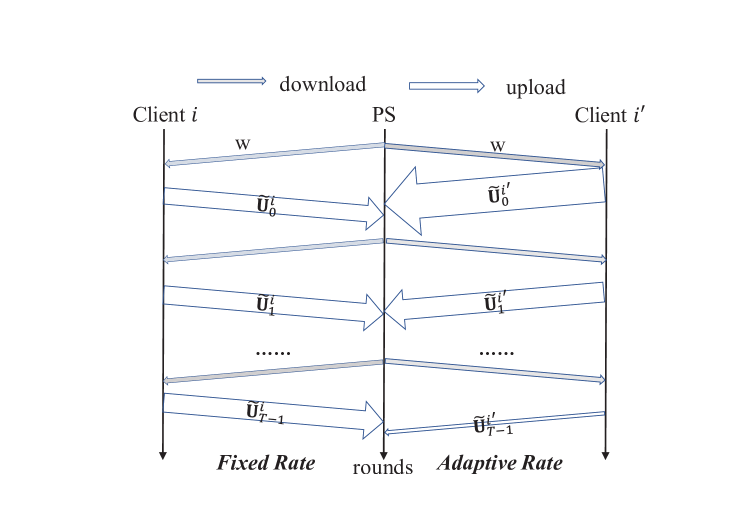
Figure 1: Transmitting model updates with a fixed compression rate (left) vs adaptive compression rates (right): the width of arrows indicates the amount of data uploaded by the client, implying different compression rates.

In Table I, we summarize the key notations used in this paper. Without loss of generality, we define the compression error as $J_{t}^{i}=\mathbb{E}\|\widetilde{\mathbf{U}}^{i}_{t}-\mathbf{U}^{i}_{t}\|^{2}$. Note that, this definition is applicable for all unbiased compression algorithms through customizing $J_{t}^{i}$. The influence of $J_{t}^{i}$ on the final model accuracy will be quantified in the next section through our convergence analysis with model compression.

TABLE I: Notation List

Notation	Meaning
$p_{i}$	the weight of client $i$ among all clients
$\mathbf{U}^{i}_{t}$	model updates of client $i$ in the $t^{th}$ global iteration
$\widetilde{\mathbf{U}}^{i}_{t}$	compressed model updates randomly generated based on $\mathbf{U}^{i}_{t}$
$Z$	number of centroids
$d$	dimensions of the model
$\mathcal{K}_{t}$	set of clients selected to participate the $t^{th}$ global iteration
$\Gamma_{c}/\Gamma_{n}$	quantified the heterogeneity of the non-IID data distribution if loss function is strongly convex/non-convex
$\mathbf{w}^{i}_{t,j}$	model updated $j$ times on client $i$ in the $t^{th}$ global iteration
$\mathbf{w}_{t}$	model downloaded from PS to clients in the $t^{th}$ global iteration

IV Convergence Analysis under Model Compression

In this section, we analyze the convergence rate of FedAvg when compressed model updates are transmitted to the PS. As in previous works [10, 28, 20, 11], we make the following assumptions on the learned models in FL.

Assumption 1.

All loss functions, i.e., $F_{1},F_{2},\dots,F_{N}$ are $L$-smooth; that is, given $\mathbf{v}$ and $\mathbf{w}$, we have $F_{i}(\mathbf{v})\leq F_{i}(\mathbf{w})+(\mathbf{v}-\mathbf{w})^{T}\nabla F_{i}(\mathbf{w})+\frac{L}{2}||\mathbf{v}-\mathbf{w}||^{2}$.

Assumption 2.

Let $\xi^{i}_{t}$ denote a sample randomly and uniformly selected from client $i$. The variance of the stochastic gradients in each client is bounded: $\mathbb{E}[\|\nabla F_{i}(\mathbf{w}^{i}_{t,j},\xi^{i}_{t,j})-\nabla F_{i}(\mathbf{w}^{i}_{t,j})\|^{2}]\leq\sigma^{2}$ for $\forall i,\forall j,\forall t$.

Assumption 3.

The expected square norm of stochastic gradients is uniformly bounded, i.e., $\mathbb{E}[\|\nabla F_{i}(\mathbf{w}^{i}_{t,j},\xi^{i}_{t,j})\|^{2}]\leq G^{2}$ for $\forall i,\forall j,\forall t$.

These assumptions hold in typical FL models, as discussed in the previous works [10, 28, 20, 11]. We also assume that the FL system uses a Partial Client Participation Mode [10], i.e., in each round of global iteration, the PS randomly selects $K$ clients according to the weight probabilities $p_{1},p_{2},\dots,p_{N}$ with replacement to conduct local iterations. The set of selected clients is denoted by $\mathcal{K}_{t}$ at the $t^{th}$ global iteration. The PS then aggregates model updates by $\mathbf{w}_{t}=\mathbf{w}_{t-1}-\frac{\eta_{t-1}}{K}\sum_{i\in\mathcal{K}_{t-1}}\widetilde{\mathbf{U}}^{i}_{t-1}$, where $\widetilde{\mathbf{U}}^{i}_{t-1}$ denotes compressed model updates.

IV-A With Strongly Convex Loss Functions

We first analyze the convergence rate by assuming that all loss functions $F_{1},F_{2},\dots,F_{N}$, are $\mu$-strongly convex; that is, given $\mathbf{v}$ and $\mathbf{w}$, we have $F_{i}(\mathbf{v})\geq F_{i}(\mathbf{w})+(\mathbf{v}-\mathbf{w})^{T}\nabla F_{i}(\mathbf{w})+\frac{\mu}{2}||\mathbf{v}-\mathbf{w}||^{2}$. In practice, most loss functions belong to this category [10, 29].

For strongly convex loss functions, we use $\Gamma_{c}=F^{*}-\sum_{i=1}^{N}p_{i}F^{*}_{i}$ to quantize the degree of non-IID sample distribution on clients. Here, $F^{*}$ and $F^{*}_{i}$ are the optimal values of $F$ and $F_{i}$, respectively.

Theorem 1.

Let $\eta_{t}=\frac{2}{\mu(t+\gamma)}$, $\gamma=\frac{8L}{\mu}$, $\kappa=\frac{L}{\mu}$ and $\mathbf{w}^{*}$ is the optimal model, the convergence rate of FedAvg with compressed unbiased model updates is

$$\autobreak\MoveEqLeft[0]\mathbb{E}\left\|\mathbf{w}_{T}-\mathbf{w}^{*}\right\|^{2}\leq$$

$$\autobreak\MoveEqLeft[0]\frac{4}{\gamma+T}\Big{(}\frac{\alpha}{\mu}+\sum_{t=0}^{T-1}\frac{\eta_{t}\sum_{i=1}^{N}p_{i}J^{i}_{t}}{2K\mu}+2\kappa\left\|\mathbf{w}_{0}-\mathbf{w}^{*}\right\|^{2}\Big{)},$$ (5)

where $\alpha=\frac{E\sum_{i=1}^{N}p_{i}^{2}\sigma^{2}}{B}+6EL\Gamma_{c}+2E(E-1)^{2}G^{2}+\frac{E^{2}G^{2}}{K}$.

The key to the proof is to construct a model for each local iteration and derive the gap between this model and the optimal model. Please refer to Appendix A for the detailed proof.

It is worth mentioning that, the compression error can be bounded by $J_{t}^{i}=\mathbb{E}\|\widetilde{\mathbf{U}}^{i}_{t}-\mathbf{U}^{i}_{t}\|^{2}\leq(1-\delta)\|\mathbf{U}_{t}^{i}\|$, where $0<\delta\leq 1$ [30]. With this bound, the convergence rate $O(\frac{1}{T})$ was proved in the work [21]. However, this bound ignores the relation between the number of centroids and the compression error, and thereby we cannot adapt compression rate based on the convergence rate derived with this bound.

Remark: We can extract term $\sum_{t=0}^{T-1}\eta_{t}\sum_{i=1}^{N}p_{i}J^{i}_{t}$ from the convergence rate, which indicates that the influence of the compression error on the final model accuracy depends on the learning rate. To maximize the final model accuracy, we should minimize $\sum_{t=0}^{T-1}\eta_{t}\sum_{i=1}^{N}p_{i}J^{i}_{t}$, and accordingly adjust the compression rates in accordance with the learning rates.

IV-B With Non-convex Loss Functions

We proceed to analyze the convergence rate when loss functions are non-convex. In this case, we use the difference between global gradients and local gradients to quantize the non-IID degree of the sample distribution on clients. That is $\Gamma_{n}\geq\mathbb{E}\|\nabla F_{i}(\mathbf{w}_{t})-\nabla F(\mathbf{w}_{t})\|^{2}$.

Theorem 2.

Let $c>0$ is a constant and a learning rate satisfying $\eta_{t}\leq\frac{1}{8LE}$, $\eta_{t}EL\leq\frac{K}{K-1}$ and $30NE^{2}\eta_{t}^{2}L^{2}\sum_{i=1}^{N}p_{i}^{2}+\frac{L\eta_{t}}{K}(90E^{3}L^{2}\eta_{t}^{2}+3E)<1$, the convergence rate of FedAvg with compressed unbiased model updates is

$$\autobreak\MoveEqLeft[0]\min_{t\in[T]}\mathbb{E}\|\nabla F(\mathbf{w}_{t})\|^{2}\leq\frac{L}{2c\eta_{T-1}TE}\sum_{t=0}^{T-1}\eta_{t}^{2}\sum_{i=1}^{N}p_{i}J^{i}_{t}$$

$$\autobreak\MoveEqLeft[0]+(\frac{LE^{2}\sigma^{2}}{2}+\frac{3E^{2}L\Gamma_{n}}{2K})\frac{\sum_{t=0}^{T-1}\eta_{t}^{2}}{c\eta_{T-1}TE}+\frac{(\sigma^{2}+6E\Gamma_{n})}{c\eta_{T-1}TE}$$

$$\autobreak\MoveEqLeft[0]\Big{[}\frac{5NE^{2}L^{2}\sum_{i=1}^{N}p_{i}^{2}\sum_{t=0}^{T-1}\eta_{t}^{3}}{2}+\frac{15E^{3}L^{3}\sum_{t=0}^{T-1}\eta_{t}^{4}}{2K}\Big{]}$$

$$\autobreak\MoveEqLeft[0]+\frac{F_{0}-F_{*}}{c\eta_{T-1}TE},$$ (6)

where $F_{0}$ and $F_{*}$ represent the initial value and optimal value of the global loss function, respectively. The key to the proof is to analyze the decrease of the loss function after each global iteration through the $L-smooth$ property. Please refer to Appendix B for the detailed proof.

Remark: It can be seen that the influence of compression error is related with $\eta_{t}^{2}$. To maximize the final model accuracy, we should minimize $\sum_{t=0}^{T-1}\eta_{t}^{2}\sum_{i=1}^{N}p_{i}J^{i}_{t}$. Again, although the convergence rate $O(\frac{1}{\sqrt{T}})$ can be found in [31], it ignores the relation between the compression error and the number of centroids and hence does not work for rate adaption.

V Optimal Rate Adaptation for Model Compression

The communication overhead of each global iteration can be quantified by the number of centroids $Z$. Suppose that each original model update takes $h$ bytes. With a compression algorithm, e.g., Probability Quantification (PQ) [7], it takes $Zh$ bytes to represent the $Z$ centroids and $\log_{2}{Z}$ bits to represent the identification of each model update. The total traffic will be $Zh+d\log_{2}{Z}$, where $d$ is the model dimension. For high-dimensional models, we have $d\gg Z$ [32]. The traffic of each global iteration is therefore approximately $\frac{d\log_{2}{Z}}{8}$ bytes. Assume transmitting the original model updates needs $hd$ bytes, the compression rate is given by $\Lambda=\frac{hd}{d\frac{\log_{2}{Z}}{8}}=\frac{8h}{\log_{2}{Z}}$.

Based on the derived convergence rates, we now establish the policy to maximize the final model accuracy by adapting compression rates in accordance with learning rates.

V-A Optimal Rate Adaptation Framework

We formulate the problem to optimize model accuracy by adapting compression rates without incurring additional communication overhead.

From Theorems 1 and 2, we can extract terms related with compression errors, and define the adaptive rate objective as:

$$\mathcal{J}=\left\{\begin{aligned} &\sum_{t=0}^{T-1}\eta_{t}\sum_{i=1}^{N}p_{i}J^{i}_{t},\quad\textit{Loss $F_{i}$ is strongly convex},\\ &\sum_{t=0}^{T-1}\eta_{t}^{2}\sum_{i=1}^{N}p_{i}J^{i}_{t},\quad\textit{Loss $F_{i}$ is non-convex}.\\ \end{aligned}\right.$$ (7)

Here $J^{i}_{t}$ is the compression error on client $i$ in the $t^{th}$ global iteration. To maximize the final model accuracy with a finite $T$, we should minimize $\mathcal{J}$. Recall that the compression error is defined as $J^{i}_{t}=\mathbb{E}\|\widetilde{\mathbf{U}}^{i}_{t}-\mathbf{U}^{i}_{t}\|^{2}$. Thus, $J_{t}^{i}$ is a function that will be affected by the number of centroids $Z_{t}$, where $Z_{t}$ should be a positive integer.

Let $d\times x_{t}$ bits be the approximate traffic with compressed model updates in the $t^{th}$ global iteration where $x_{t}=\log_{2}{Z_{t}}$. Let $\mathbf{x}=(x_{0},\dots,x_{T-1})$, the total traffic will be $d\times\|\mathbf{x}\|_{1}$, which can be bounded by a constant $C$.

We then have the following integer programming problem:

$$\mathbb{P}1: \min_{Z_{0},\dots,Z_{T-1}}\mathcal{J}$$ (8)

$$s.t.\quad\|\mathbf{x}\|_{1}\leq\frac{C}{d}$$

$$\qquad Z_{t}=\{1,2,\dots\}\quad\textit{for $t=0,\dots,T-1$.}$$

Due to the difficulty to solve an integer programming problem, we relax the constraint to allow $Z_{t}$ to be a real positive number. Then, we can formulate the following problem.

$$\mathbb{P}2: \min_{Z_{0},\dots,Z_{T-1}}\mathcal{J}$$ (9)

$$s.t.\quad\|\mathbf{x}\|_{1}\leq\frac{C}{d}$$

$$\qquad Z_{t}\geq 1\quad\textit{for $t=0,\dots,T-1$.}$$

Since $Z_{t}$ is a real number, we can solve $\mathbb{P}2$ through gradient descent algorithm [33], and then each solved $Z_{t}$ can be rounded to its nearest integer.

V-B Implementation Issues

To implement our adaption framework, such information as $\eta_{t}$, $p_{i}$, and $C$ are to be obtained by the PS. The learning rate $\eta_{t}$ can be reported by clients, which only takes 4 bytes in each communication round; The weight $p_{i}$ (usually proportional to the sample population owned by client $i$) and the restriction of communication traffic $C$ can be determined prior to the model training. After solving problem $\mathbb{P}2$, the PS can send out the adaptive compression rate $Z_{t}$ (a single number) together with the latest model parameters to participating clients in each communication round.

Our framework is applicable with various unbiased compression algorithms in FL. In practice, we need to derive the expression of $J_{t}^{i}$ with specified compression algorithms. To demonstrate the usability of our framework, we conduct a case study with two widely used compression algorithms for FL, namely, Probability Quantization [12] and Quantized SGD [13].

V-B1 Case Study with Probability Quantization (PQ)

The PQ algorithm uses $Z$ centroids to split a certain range into $Z-1$ intervals. The model update in an interval will be probabilistically quantified in an unbiased manner to the upper or lower centroids of the interval. According to [12], the compression error can be bounded as follows.

$$J^{i}_{t} = \mathbb{E}\left\|\widetilde{\mathbf{U}}^{i}_{t}-\mathbf{U}^{i}_{t}\right\|^{2}$$ (10)

$$\overset{(1)}{\leq} \frac{d(U_{max}-U_{min})^{2}}{4(Z-1)^{2}}\leq\frac{d(2U^{2}_{max}+2U^{2}_{min})}{4(Z-1)^{2}}$$

$$\leq \frac{2d\|\mathbf{U}_{t}^{i}\|^{2}}{4(Z-1)^{2}}=\frac{d\|\sum_{j=0}^{E-1}\nabla F_{i}(\mathbf{w}^{i}_{t,j},\mathcal{B}^{i}_{t,j})\|^{2}}{2(Z_{t}-1)^{2}}$$

$$\overset{(2)}{\leq} \frac{dE^{2}G^{2}}{2(Z_{t}-1)^{2}}=\frac{dE^{2}G^{2}}{2(2^{x_{t}}-1)^{2}},$$

where $U_{max}$ and $U_{min}$ are the maximum and minimum values of each element in vector $\mathbf{U}_{t}^{i}$, respectively. Here, inequality $(1)$ is adapted from Theorem 2 in [12] and inequality $(2)$ is from Assumption 3.

It can be verified that $J_{t}^{i}$ defined in Eq.(10) is convex with respect to $x_{t}$. Substituting Eq.(10) into $\mathbb{P}2$, we can solve $x_{t}$, and hence $Z_{t}$.

V-B2 Case Study with Quantized SGD (QSGD)

Quantized SGD (QSGD) is another popular unbiased compression algorithm in FL. Let $\mathbf{U}$ denote an arbitrary model update vector and $U_{e}$ denote an arbitrary element in $\mathbf{U}$. $U_{e}$ is quantified to $Q(U_{e})$ by $Q(U_{e})=\|\mathbf{U}\|^{2}*sgn(U_{e})*\xi_{e},$ where $sgn(U_{e})$ is the sign of $U_{e}$ and $\xi_{e}$ is a random variable affected by $U_{e}$. We can control $\xi_{e}$ such that $\mathbb{E}[Q(U_{e})]=U_{e}$, and the compression error of QSGD is bounded in [13], which is

$$J^{i}_{t} =\mathbb{E}\Big{\|}\widetilde{\mathbf{U}}^{i}_{t}-\mathbf{U}^{i}_{t}\Big{\|}^{2}\ \overset{(1)}{\leq}\ \min(\frac{d}{Z_{t}^{2}},\frac{\sqrt{d}}{Z_{t}})\|\mathbf{U}^{i}_{t}\|^{2}$$ (11)

$$=\min(\frac{d}{Z_{t}^{2}},\frac{\sqrt{d}}{Z_{t}})\Big{\|}\sum_{j=0}^{E-1}\nabla F_{i}(\mathbf{w}^{i}_{t,j},\mathcal{B}^{i}_{t,j})\Big{\|}^{2}$$

$$\leq\min(\frac{dE^{2}G^{2}}{Z_{t}^{2}},\frac{\sqrt{d}E^{2}G^{2}}{Z_{t}})=\min(\frac{dE^{2}G^{2}}{2^{2x_{t}}},\frac{\sqrt{d}E^{2}G^{2}}{2^{x_{t}}}),$$

where inequality $(1)$ is from Lemma 3.1 in [13]. Again, Eq. (11) is convex with respect to $x_{t}$. By substituting Eq. (11) into the problem $\mathbb{P}2$, we can optimally determine $x_{t}$ and $Z_{t}$.

VI Performance Evaluation

We have conducted extensive experiments to evaluate the effectiveness in terms of model accuracy, communication traffic and communication time by adaptive compression rates. In this section, we report our key findings with two representative datasets, namely, MNIST and CIFAR-10 [14], for convex loss and non-convex loss, respectively.

1. Convex Loss Case - MNIST [9, 11]: The MNIST dataset contains 70,000 hand-written digital images with labels 0-9. Each sample is a 28×28 grayscale image. We randomly select 60,000 images as the training set and use the rest 10,000 images as the test set. We train a logistic regression model (which is convex) to classify the MNIST datasets. The model contains a fully connected layer with 784 inputs and 10 outputs (without activation function), and therefore involves 7,850 parameters in total. Similar to [10], we set the learning rate as $\frac{0.01}{1+t*E}$, where $t$ is the global iteration index.

2. Non-Convex Loss Case - CIFAR-10: The CIFAR-10 dataset consists of 60,000 32×32 color images, which belong to 10 classes. We randomly select 50,000 images as the training set and 10,000 images as the test set. We train a convolutional neural network (CNN) model (which is non-convex). The CNN model has three 3×3 convolutional layers. For the first two layers, each layer is followed by a max pooling layer; there are two fully connected layers for the output of 10 classes of probabilities. A similar model structure has been used in [34, 2] with 122,570 parameters in total. We set the learning rate as $\frac{0.05}{1+\sqrt{t*E}/40}$ according to Theorem 2.

In our experiments, we set up 100 clients and a single PS in the FL system and implement the FedAvg algorithm in [2] for model training. In each round of communication, the PS will randomly select 10 participating clients and each client is selected with the probability proportional to the number of samples owned by the client. Selected clients will download the latest model parameters from the PS and conduct $E=5$ local iterations. For local iterations, we use the batch gradient descent algorithm [35], and the batch size is set as 50 and 8 for convex and non-convex loss functions, respectively. These default parameter settings resemble those used in previous study [2]. The total numbers of global iterations for training convex and non-convex loss functions are 200 and 400, respectively.

We have implemented both the Adaptive PQ and the Adaptive QSGD algorithms to compress model updates based on our case discussion in the previous section. The standard PQ and QSGD therefore serve as the baselines for comparison. FedAvg (without compression) is implemented to evaluate how the model accuracy will be impacted by compression errors. We have also implemented an Adaptive TopK compression algorithm to evaluate the robustness of our framework. It is derived from the well-known TopK biased compression algorithm [30], which only selects the $K$ model updates that are furthest away from $0$ for transmission.

We evaluate compression algorithms from three critical perspectives, namely, model accuracy, communication traffic, and communication time.

VI-A Comparison of Model Accuracy

We start from the accuracy results with MNIST, i.e., the convex loss case. We adopt both IID and non-IID sample distributions for our experiments: (1) IID distribution, which randomly allocates 600 samples from the training set to each client; and (2) Non-IID distribution, which randomly allocates 600 samples out of 5 classes from the training set to each client.

For PQ and QSGD, we set the default $Z$, i.e., the number of centroids, to be 16 for compression in each global iteration. Given total 200 global iterations, for both Adaptive PQ and Adaptive QSGD, we have the total traffic limitation $C=\sum_{t=0}^{T=199}d\times\log_{2}Z_{t}=200d\times\log_{2}{16}=800d$ bits to ensure a fair comparison for different compression algorithms.

The results of our experiments are shown in Figs. 2 for PQ and 3 for QSGD. The x-axis represents the number of global iterations, while the y-axis represents the model accuracy on the test dataset. From the results in Figs. 2 and 3, one can observe that adaptive algorithms achieve higher model accuracy in all experimental cases, which also shed light on the effectiveness of our framework.

Note that, although Adaptive PQ and Adaptive QSGD can reach over 87% model accuracy, it is a little bit less than the accuracy of FedAvg without compression because the model compression operation inevitably lowers the model accuracy. The traffic however is reduced significantly with compression, around $32/\log_{2}{16}=8$ times less than the original, assuming each original model update takes $4$ bytes.

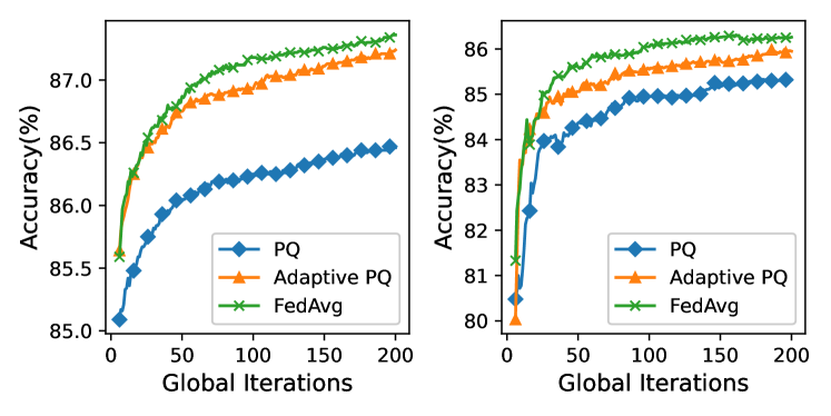
Figure 2: Accuracy comparison of Adaptive PQ and PQ in MNIST with IID (left) and non-IID (right) sample distributions (Our plotting starts from the $5^{th}$ global iteration).

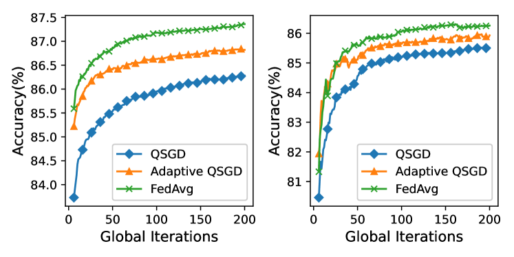
Figure 3: Accuracy comparison of Adaptive QSGD and QSGD in MNIST with IID (left) and non-IID (right) sample distributions (Our plotting starts from the $5^{th}$ global iteration).

We have conducted similar experiments with the CIFAR-10 dataset, i.e., non-convex case. Again, we implement two sample distributions: (1) IID distribution, which randomly allocates 500 samples from the training set to each client; and (2) Non-IID distribution, which randomly allocates 500 samples out of 5 classes from the training set to each client.

For both PQ and QSGD, we set $Z=128$. For Adaptive PQ and Adaptive QSGD, it implies that $C=\sum_{t=0}^{T=399}d\times\log_{2}{Z_{t}}=400d\times\log_{2}{128}=2800d$ bits with 400 global iterations.

The experiment results are presented in Figs. 4 for PQ and 5 for QSGD. From the experimental results, we can observe that Adaptive PQ and Adaptive QSGD can achieve higher model accuracy even if the loss functions are non-convex. Compared to the results of MNIST, the model accuracy in Figs. 4 and 5 fluctuates more frequently because the classification task of the CIFAR-10 dataset is more complicated. Nevertheless, the model accuracy of our adaptive algorithms is only slightly lower than that of FedAvg without compression, and adapting compression rates always achieves higher model accuracy than fixed rate compression algorithms, demonstrating the superiority of our framework.

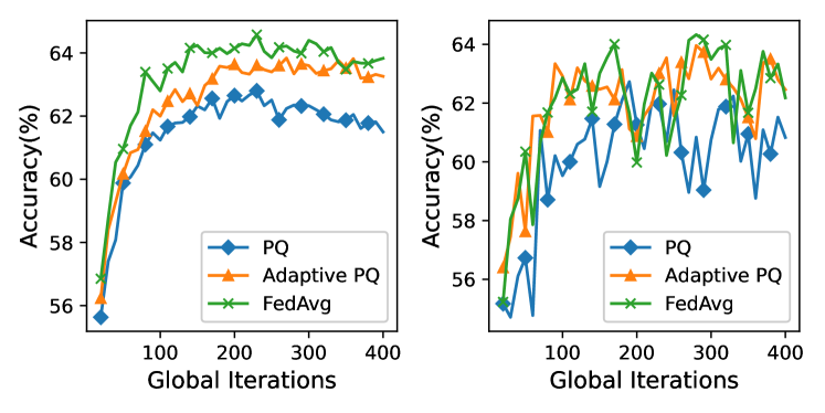
Figure 4: Accuracy comparison of Adaptive PQ and PQ in CIFAR-10 with IID (left) and non-IID (right) sample distributions (Our plotting starts from the $20^{th}$ global iteration).

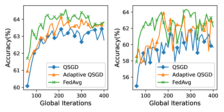
Figure 5: Accuracy comparison of Adaptive QSGD and QSGD in CIFAR-10 with IID (left) and non-IID (right) sample distributions (Our plotting starts from the $60^{th}$ global iteration).

VI-B Evaluating Robustness

Although our theoretical analysis has focused on unbiased compression, we believe that our framework is also applicable to biased compression because, in this case, the influence to the final model accuracy is related with the learning rate as well.

In our Adaptive TopK algorithm, let $K_{t}$ denote the number of selected model updates in round $t$, then the error function of TopK is $J^{i}_{t}=\mathbb{E}\|\widetilde{\mathbf{U}}^{i}_{t}-\mathbf{U}^{i}_{t}\|\leq(1-K_{t}/d)\mathbf{U}^{i}_{t}$ [30]. By substituting it into $\mathbb{P}2$, we can determine the $K_{t}$ (i.e., $Z_{t}$) for Adaptive TopK. We compare the model accuracy between Adaptive TopK and TopK with MNIST and CIFAR-10. The sample distributions are non-IID, same as the non-IID distributions in previous experiments.

To restrict the total communication traffic, we set $K=3\%d$ for MNIST and $K=1\%d$ for CIFAR-10 for the TopK algorithm. In our experiments, each model update consumes 32 bits. The traffic limit $C$ for Adaptive TopK is $\sum_{t=0}^{T=199}{K_{t}}\times(32+\log_{2}d)=6d\times(32+\log_{2}d)$ bits for MNIST where $\log_{2}d$ bits are used to indicate the index of each transmitted model update. Similarly, we have $C=\sum_{t=0}^{T=399}K_{t}\times(32+\log_{2}d)=4d\times(32+\log_{2}d)$ bits for CIFAR-10.

The experimental results are presented in Fig. 6 showing that Adaptive TopK significantly outperforms TopK in terms of model accuracy. Note that the model accuracy of TopK and Adaptive TopK is lower than that of FedAvg, because the compression rate of TopK is very high. This will be further verified in the next experiment on traffic consumption.

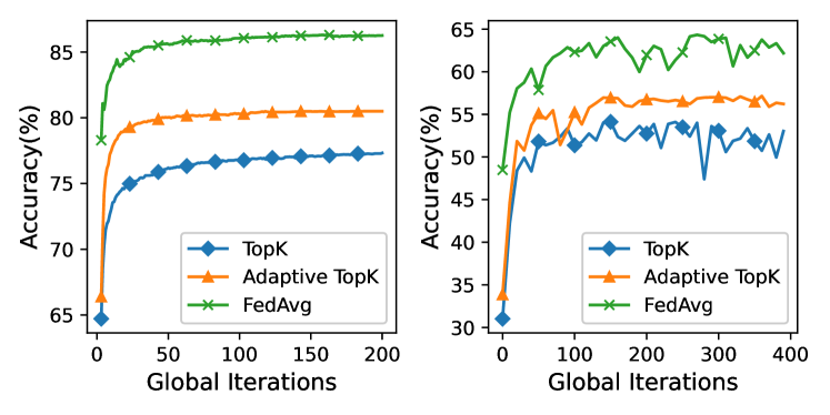
Figure 6: Accuracy comparison of Adaptive TopK and TopK in MNIST (left) and CIFAR-10 (right) with non-IID sample distributions.

VI-C Comparison of Communication Traffic and Time

We have implemented a network simulator [36].

To evaluate the consumed total communication traffic and the communication time towards the target accuracy, we simulated wireless communications based on LTE networks, and use the urban channel model defined in the ITU-R M.2135-1 for Micro NLOS communication [37]. In the network, the antenna heights of the PS and clients are 11m and 1m, and the antenna gains are 20dBm and 0dBi, respectively. The carrier frequency is 2.5GHz and 10 resource blocks are allocated to a client in each 0.5ms time slot. Under these settings, the average uplink throughput of clients is 1.4 Mbit/s. To emulate the dynamics in real networks, the network speed is sampled from the Gaussian Distribution and its standard deviation is 10% of the mean throughput. The communication time in the $t^{th}$ round is estimated as $\max_{k\in\mathcal{K}_{t}}\frac{M}{\theta_{k}}$, where $\theta_{k}$ is the network speed of client $k$ and $M$ is the traffic.

TABLE II: Comparison of total uplink communication traffic and communication time from clients to the PS between fixed and adaptive compression algorithms with non-IID distribution

Alg.	DataSet	Target Accu.	Traffic(MB)		Comm. Time(s)
			Fixed	Adap.	Fixed	Adap.
PQ	MNIST	85%	5.0	1.9	3.4	1.3
	CIFAR-10	62%	173.9	94.0	117.7	89.9
QSGD	MNIST	85%	2.4	1.6	1.6	1.1
	CIFAR-10	61.5%	255.7	175.9	172.8	156.0
TopK	MNIST	77%	1.7	0.2	1.1	0.1
	CIFAR-10	54.5%	21.1	10.9	14.3	7.4
FedAvg	MNIST	85%	7.2		5.0
	CIFAR-10	62%	374.1		258.2

We evaluate the consumed total uplink communication traffic from clients to the PS and the total communication time towards the target accuracy. Based on the experiments with non-IID sample distributions in Figs. 2-6, we present the comparison results in Table II. The results in Table II shows the tradeoff between model accuracy and the compression rate. FedAvg without compression consumes much more communication traffic and longer training time than other algorithms though its accuracy is slightly higher. Our adaptive algorithms always consume less communication traffic and communication time than algorithms with fixed compression rates. The model accuracy of TopK is slightly lower, but it consumes much less communication traffic and communication time than PQ and QSGD. It is worth noting that Adaptive TopK can further reduce the traffic and time cost of Fixed TopK.

VII Conclusion

Federated learning involves heavy data communication across distributed network nodes. Compression is necessary for FL over today’s capacity limited and dynamic Internet and wireless networks. In this paper, we for the first time analyzed the convergence rate of FedAvg with adaptive compression for both strongly convex and non-convex loss functions. We presented an optimized framework that balances the compression rates with learning rates, seeking to maximize the overall model accuracy. Our rate adaptation framework is generally applicable with diverse compression algorithms, and we have closely examine the implementation with PQ and QSGD. Experiment results with such representative datasets as MNIST and CIFAR-10 suggested that our solution effectively reduces network traffic yet maintains high model accuracy in FL.

Our work is an initial attempt toward this direction and there remain spaces to explore. In particular, with advances in compression algorithms, it can be difficult to derive an exact expression of $J_{t}^{i}$ for a future algorithm. A possible solution is to fit the compression error function with different compression rates. This trial process is lightweight in communication since the PS only needs to communicate parameters of the fitting function with clients. We will investigate its effectiveness in theory as well conduct larger scale experiments to further optimize our solutions.

Appendix A Proof of Theorem 1

We use $\mathbf{v}^{i}_{t,j+1}=\mathbf{w}^{i}_{t,j}-\eta_{t}\nabla F_{i}(\mathbf{w}^{i}_{t,j},\mathcal{B}^{i}_{t,j})$ to represent the result of a local epoch result on client $i$, whereas $\mathbf{w}^{i}_{t,j+1}=\mathbf{v}^{i}_{t,j+1}$ if $j+1<E$, else, $\mathbf{w}^{i}_{t+1,0}=\mathbf{w}^{i}_{t,0}-\frac{\eta_{t}}{K}\sum_{i\in\mathcal{K}_{t}}\widetilde{\mathbf{U}}^{i}_{t}$ and $\mathbf{v}^{i}_{t+1,0}=\mathbf{v}^{i}_{t,E}$. We further define $\bar{\mathbf{v}}_{t,j}=\sum_{i=1}^{N}p_{i}\mathbf{v}^{i}_{t,j}$, $\bar{\mathbf{w}}_{t,j}=\sum_{i=1}^{N}p_{i}\mathbf{w}^{i}_{t,j}$, $\bar{\mathbf{v}}_{t}=\bar{\mathbf{v}}_{t,0}$ and $\bar{\mathbf{w}}_{t}=\bar{\mathbf{w}}_{t,0}$.

Lemma 1.

Let Assumptions 1-3 hold, $\eta_{t}\leq\frac{1}{4L}$, we have $\mathbb{E}\left\|\bar{\mathbf{v}}_{t,j+1}-\mathbf{w}^{*}\right\|^{2}=(1-\eta_{t}\mu)\mathbb{E}\left\|\bar{\mathbf{w}}_{t,j}-\mathbf{w}^{*}\right\|^{2}+\eta_{t}^{2}\frac{1}{B}\sum_{i=1}^{N}p_{i}^{2}\sigma^{2}+6L\eta_{t}^{2}\Gamma_{c}+2\eta_{t}^{2}(E-1)^{2}G^{2}.$

Lemma 2.

Let Assumptions 1-3 hold, we have $\mathbb{E}[\bar{\mathbf{w}}_{t,j}]=\bar{\mathbf{v}}_{t,j}.$

Lemma. 1-2 has been proved in [10].

When Assumptions 1-3 hold, we will analyze the variance between $\bar{\mathbf{v}}_{t+1}$ and $\bar{\mathbf{w}}_{t+1}$ as follow.

$$\mathbb{E}\left\|\bar{\mathbf{w}}_{t+1}-\bar{\mathbf{v}}_{t+1}\right\|^{2}=\mathbb{E}\Big{\|}\frac{\eta_{t}}{K}\sum_{i\in\mathcal{K}_{t}}\widetilde{\mathbf{U}}^{i}_{t}-\eta_{t}\sum_{i=1}^{N}p_{i}\mathbf{U}^{i}_{t}\Big{\|}^{2}$$

$$=\frac{\eta_{t}^{2}}{K^{2}}\mathbb{E}\big{[}\big{\|}\sum_{l=1}^{K}\big{(}\widetilde{\mathbf{U}}^{i_{l}}_{t}-\sum_{i=1}^{N}p_{i}\mathbf{U}^{i}_{t}\big{)}\big{\|}^{2}\big{]}$$

$$=\frac{\eta_{t}^{2}}{K^{2}}\sum_{l=1}^{K}\mathbb{E}\Big{[}\Big{\|}\widetilde{\mathbf{U}}^{i_{l}}_{t}-\sum_{i=1}^{N}p_{i}\mathbf{U}^{i}_{t}\Big{\|}^{2}\Big{]}$$

$$=\frac{\eta_{t}^{2}}{K}\sum_{i^{{}^{\prime}}=1}^{N}p_{i^{{}^{\prime}}}\mathbb{E}\Big{\|}\widetilde{\mathbf{U}}^{i^{{}^{\prime}}}_{t}-\sum_{i=1}^{N}p_{i}\mathbf{U}^{i}_{t}\Big{\|}^{2}$$

$$=\frac{\eta_{t}^{2}}{K}\sum_{i^{{}^{\prime}}=1}^{N}p_{i^{{}^{\prime}}}\mathbb{E}\Big{[}\Big{\|}\widetilde{\mathbf{U}}^{i^{{}^{\prime}}}_{t}-\mathbf{U}^{i^{{}^{\prime}}}_{t}\Big{\|}^{2}+\Big{\|}\sum_{i=1}^{N}p_{i}\mathbf{U}^{i}_{t}-\mathbf{U}^{i^{{}^{\prime}}}_{t}\Big{\|}^{2}\Big{]}$$

$$\leq\frac{1}{K}\sum_{i^{{}^{\prime}}=1}^{N}p_{i^{{}^{\prime}}}\eta_{t}^{2}J^{i^{\prime}}_{t}+\frac{\eta_{t}^{2}}{K}\mathbb{E}\Big{[}\sum_{i^{{}^{\prime}}=1}^{N}p_{i^{{}^{\prime}}}\left\|\mathbf{U}^{i^{{}^{\prime}}}_{t+1}\right\|^{2}\Big{]}$$

$$\leq\frac{1}{K}\sum_{i^{{}^{\prime}}=1}^{N}p_{i^{{}^{\prime}}}\eta_{t}^{2}J^{i^{\prime}}_{t}+\frac{\eta_{t}^{2}G^{2}E^{2}}{K}.$$

We will use the lemmas to derive the convergence of the model. We first analyze the interval between $\bar{\mathbf{w}}_{t+1}$ and $\mathbf{w}^{*}$.

$$\begin{split}&\mathbb{E}\left\|\bar{\mathbf{w}}_{t+1}-\mathbf{w}^{*}\right\|^{2}=\mathbb{E}\left\|\bar{\mathbf{w}}_{t+1}-\bar{\mathbf{v}}_{t+1}+\bar{\mathbf{v}}_{t+1}-\mathbf{w}^{*}\right\|^{2}\\ &\leq(1-\eta_{t}\mu)\left\|\bar{\mathbf{w}}_{t,E-1}-\mathbf{w}^{*}\right\|^{2}+\eta_{t}^{2}\tau+\eta_{t}^{2}\frac{E^{2}G^{2}}{K}+\psi_{t},\end{split}$$

where $\tau=\frac{\sum_{i=1}^{N}p_{i}^{2}\sigma^{2}}{B}+6L\Gamma_{c}+2(E-1)^{2}G^{2}$ and $\psi_{t}=\frac{1}{K}\sum_{i=1}^{N}p_{i}\eta_{t}^{2}J^{i}_{t}$. According to Lemma 1 and $\bar{\mathbf{w}}^{i}_{t,j}=\bar{\mathbf{v}}^{i}_{t,j}$, we can get $\mathbb{E}\left\|\bar{\mathbf{w}}_{t,j+1}-\mathbf{w}^{*}\right\|^{2}\leq(1-\eta_{t}\mu)\left\|\bar{\mathbf{w}}_{t,j}-\mathbf{w}^{*}\right\|^{2}+\eta_{t}^{2}\tau$, where $j<E-1$. Through accumulation, we can obtain

$$\mathbb{E}\left\|\bar{\mathbf{w}}_{t+1}-\mathbf{w}^{*}\right\|^{2}\leq(1-\eta_{t}\mu)\mathbb{E}\left\|\bar{\mathbf{w}}_{t}-\mathbf{w}^{*}\right\|^{2}+\eta_{t}^{2}\alpha+\psi_{t},$$

where $\alpha=\frac{E\sum_{i=1}^{N}p_{i}^{2}\sigma^{2}}{B}+6EL\Gamma_{c}+2E(E-1)^{2}G^{2}+\frac{E^{2}G^{2}}{K}$.

For a decreasing learning rate $\eta_{t}=\frac{\beta}{t+\gamma}$ where $\beta>\frac{1}{\mu}$ and $\gamma>0$, we now prove via induction that $\mathbb{E}\left\|\bar{\mathbf{w}}_{t}-\mathbf{w}^{*}\right\|^{2}\leq\frac{\sum_{i=0}^{t-1}[(i+1+\gamma)\psi_{i}]+v}{\gamma+t}$ where $v=\max\left\{\frac{\beta^{2}\alpha}{\beta\mu-1},\gamma\left\|\bar{\mathbf{w}}_{0}-\mathbf{w}^{*}\right\|^{2}\right\}$.

Note that the inequality above holds when $t=0$ and we assume that there is $t$ that makes the inequality valid,

$$\mathbb{E}\left\|\bar{\mathbf{w}}_{t+1}-\mathbf{w}^{*}\right\|^{2}\leq(1-\eta_{t}\mu)\mathbb{E}\left\|\bar{\mathbf{w}}_{t}-\mathbf{w}^{*}\right\|^{2}+\eta_{t}^{2}\alpha+\psi_{t}$$

$$\leq(1-\frac{\beta\mu}{t+\gamma})\frac{\sum_{i=0}^{t-1}[(i+1+\gamma)\psi_{i}]+v}{\gamma+t}+\frac{\beta^{2}\alpha}{(t+\gamma)^{2}}+\psi_{t}$$

$$\leq\frac{(t+\gamma-1)}{(t+\gamma)^{2}}v+\Big{[}\frac{\beta^{2}\alpha}{(t+\gamma)^{2}}-\frac{(\beta\mu-1)}{(t+\gamma)^{2}}v\Big{]}$$

$$\qquad+\frac{t+\gamma-\beta\mu}{t+\gamma}\frac{\sum_{i=0}^{t-1}((i+1+\gamma)\psi_{i})}{t+\gamma}+\psi_{t}$$

$$\leq\frac{1}{t+\gamma+1}v+\frac{t+\gamma-1}{(t+\gamma)^{2}}\sum_{i=0}^{t-1}\big{(}(i+1+\gamma)\psi_{i}\big{)}+\psi_{t}$$

$$\leq\frac{v_{t+1}}{\gamma+t+1}.$$ (12)

Let $\beta=\frac{2}{\mu}$, $\gamma=\frac{8L}{\mu}$ and $\kappa=\frac{L}{\mu}$, we have

$$\mathbb{E}\left\|\bar{\mathbf{w}}_{T}-\mathbf{w}^{*}\right\|^{2}\leq\frac{\sum_{i=0}^{T-1}[(i+1+\gamma)\psi_{i}]+v}{\gamma+T}$$

$$\leq\frac{\frac{\beta^{2}\alpha}{\beta\mu-1}+\sum_{i=0}^{T-1}[(i+1+\gamma)\psi_{i}]+\gamma\left\|\bar{\mathbf{w}}_{0}-\mathbf{w}^{*}\right\|^{2}}{\gamma+T}$$

$$=\frac{\frac{4\alpha}{\mu}+\sum_{t=0}^{T-1}\frac{4\sum_{i=1}^{N}p_{i}J^{i}_{t}}{(t+\gamma)K\mu^{2}}+8\kappa\left\|\bar{\mathbf{w}}_{0}-\mathbf{w}^{*}\right\|^{2}}{\gamma+T}.$$ (13)

Appendix B Proof of Theorem 2

The following two lemmas adapted from [11] will be used to derive the convergence rate with non-convex loss.

Lemma 3.

Given assumptions 1 and 2 and learning rate $\eta_{t}\leq\frac{1}{8LE}$, we have $\mathbb{E}\Big{\|}\sum_{k=0}^{j-1}\nabla F_{i}(\mathbf{w}^{i}_{t,k},\mathcal{B}^{i}_{t,k})\Big{\|}^{2}\leq 5E\eta_{t}^{2}(\sigma^{2}+6E\Gamma_{n})+30E^{2}\eta_{t}^{2}\|\nabla F(\mathbf{w}_{t})\|^{2}.$

Lemma 4.

After defining $\mathbf{t}^{i}_{t}=\sum_{j=0}^{E-1}\nabla F_{i}(\mathbf{w}^{i}_{t,j})$, we have

$$\mathbb{E}\|\sum_{i\in\mathcal{K}_{t}}\mathbf{t}^{i}_{t}\|^{2}=K\sum_{i=1}^{N}p_{i}\mathbb{E}\left\|\mathbf{t}^{i}_{t}\right\|^{2}+K(K-1)\mathbb{E}\|\sum_{i=1}^{N}p_{i}\mathbf{t}^{i}_{t}\|^{2}.$$

We will use the aforementioned lemmas to derive the convergence of the model. Given Assumption 1, we have

$$\mathbb{E}[F(\mathbf{w}_{t+1})]=F(\mathbf{w}_{t})+\frac{L}{2}\mathbb{E}\Big{\|}\frac{\eta_{t}}{K}\sum_{i\in\mathcal{K}_{t}}\widetilde{\mathbf{U}}^{i}_{t}\Big{\|}^{2}+\nabla F(\mathbf{w}_{t})^{T}$$ (14)

$$\qquad\mathbb{E}\Big{[}\frac{-\eta_{t}\sum_{i\in\mathcal{K}_{t}}\widetilde{\mathbf{U}}^{i}_{t}}{K}+\eta_{t}E\nabla F(\mathbf{w}_{t})-\eta_{t}E\nabla F(\mathbf{w}_{t})\Big{]}$$

$$\qquad=F(\mathbf{w}_{t})-\eta_{t}E\|\nabla F(\mathbf{w}_{t})\|^{2}+\frac{L}{2}\mathbb{E}\Big{\|}\frac{\eta_{t}}{K}\sum_{i\in\mathcal{K}_{t}}\widetilde{\mathbf{U}}^{i}_{t}\Big{\|}^{2}$$

$$\qquad+\nabla F(\mathbf{w}_{t})^{T}\mathbb{E}\Big{[}\frac{-\eta_{t}\sum_{i\in\mathcal{K}_{t}}\widetilde{\mathbf{U}}^{i}_{t}}{K}+\eta_{t}E\nabla F(\mathbf{w}_{t})\Big{]}.$$

The last term in the above formula can be evaluated as:

$$\nabla F(\mathbf{w}_{t})^{T}\mathbb{E}\Big{[}\frac{-\eta_{t}\sum_{i\in\mathcal{K}_{t}}\widetilde{\mathbf{U}}^{i}_{t}}{K}+\eta_{t}E\nabla F(\mathbf{w}_{t})\Big{]}$$

$$=\nabla F(\mathbf{w}_{t})^{T}\mathbb{E}\Big{[}-\eta_{t}\sum_{i=1}^{N}p_{i}\mathbf{U}^{i}_{t}+\eta_{t}E\nabla F(\mathbf{w}_{t})\Big{]}$$

$$=\sqrt{\eta_{t}E}\nabla F(\mathbf{w}_{t})^{T}$$

$$\quad-\frac{\sqrt{\eta_{t}}}{\sqrt{E}}\mathbb{E}\Big{[}\sum_{i=1}^{N}p_{i}\sum_{j=0}^{E-1}\left(\nabla F_{i}(\mathbf{w}^{i}_{t,j})-\nabla F_{i}(\mathbf{w}_{t})\right)\Big{]}$$

$$\overset{(1)}{=}\frac{\eta_{t}E}{2}\|\nabla F(\mathbf{w}_{t})\|^{2}-\frac{\eta_{t}}{2E}\mathbb{E}\Big{\|}\sum_{i=1}^{N}p_{i}\sum_{j=0}^{E-1}\nabla F_{i}(\mathbf{w}^{i}_{t,j})\Big{\|}^{2}$$

$$\quad+\frac{\eta_{t}}{2E}\mathbb{E}\Big{\|}\sum_{i=1}^{N}p_{i}\sum_{j=0}^{E-1}\left(\nabla F_{i}(\mathbf{w}^{i}_{t,j})-\nabla F_{i}(\mathbf{w}_{t})\right)\Big{\|}^{2}$$

$$\leq\frac{\eta_{t}E}{2}\|\nabla F(\mathbf{w}_{t})\|^{2}-\frac{\eta_{t}}{2E}\mathbb{E}\Big{\|}\sum_{i=1}^{N}p_{i}\sum_{j=0}^{E-1}\nabla F_{i}(\mathbf{w}^{i}_{t,j})\Big{\|}^{2}$$

$$\quad+\frac{\eta_{t}NL^{2}}{2}\sum_{i=1}^{N}p_{i}^{2}\sum_{j=0}^{E-1}\mathbb{E}\left\|\mathbf{w}^{i}_{t,j}-\mathbf{w}_{t}\right\|^{2},$$ (15)

where $(1)$ is derived from $\mathbf{x}^{T}\mathbf{y}=\frac{\|\mathbf{x}\|^{2}+\|\mathbf{y}\|^{2}-\|(\mathbf{x}-\mathbf{y})\|^{2}}{2}$.

The third term in Eq. (14) can be evaluated as:

$$\mathbb{E}\big{\|}\frac{\eta_{t}}{K}\sum_{i\in\mathcal{K}_{t}}\widetilde{\mathbf{U}}^{i}_{t}\big{\|}^{2}=\frac{\eta_{t}^{2}}{K^{2}}\mathbb{E}\big{\|}\sum_{i\in\mathcal{K}_{t}}\widetilde{\mathbf{U}}^{i}_{t}\big{\|}^{2}$$

$$=\frac{\eta_{t}^{2}}{K^{2}}\mathbb{E}\big{(}\big{\|}\sum_{i\in\mathcal{K}_{t}}\big{(}\widetilde{\mathbf{U}}^{i}_{t}-\mathbf{U}^{i}_{t}\big{)}\big{\|}^{2}+\big{\|}\sum_{i\in\mathcal{K}_{t}}\sum_{j=0}^{E-1}\nabla F_{i}(\mathbf{w}^{i}_{t,j})\big{\|}^{2}\big{)}$$

$$\quad+\frac{\eta_{t}^{2}}{K^{2}}\mathbb{E}\Big{\|}\sum_{i\in\mathcal{K}_{t}}\sum_{j=0}^{E-1}\left(\nabla F_{i}(\mathbf{w}^{i}_{t,j},\mathcal{B}^{i}_{t,j})-\nabla F_{i}(\mathbf{w}^{i}_{t,j})\right)\Big{\|}^{2}$$

$$\leq\eta_{t}^{2}(\sum_{i=1}^{N}p_{i}J^{i}_{t}+E^{2}\sigma^{2})+\frac{\eta_{t}^{2}}{K^{2}}\mathbb{E}\Big{\|}\sum_{i\in\mathcal{K}_{t}}\sum_{j=0}^{E-1}\nabla F_{i}(\mathbf{w}^{i}_{t,j})\Big{\|}^{2}$$

$$\leq\eta_{t}^{2}\sum_{i=1}^{N}p_{i}J^{i}_{t}+\frac{\eta_{t}^{2}}{K}\sum_{i=1}^{N}p_{i}\mathbb{E}\Big{\|}\sum_{j=0}^{E-1}\nabla F_{i}(\mathbf{w}^{i}_{t,j})\Big{\|}^{2}$$ (16)

$$\quad+E^{2}\eta_{t}^{2}\sigma^{2}+\frac{\eta_{t}^{2}(K-1)}{K}\mathbb{E}\Big{\|}\sum_{i=1}^{N}p_{i}\sum_{j=0}^{E-1}\nabla F_{i}(\mathbf{w}^{i}_{t,j})\Big{\|}^{2}.$$

We next evaluate the second term in the above formula.

$$\mathbb{E}\Big{\|}\sum_{j=0}^{E-1}\nabla F_{i}(\mathbf{w}^{i}_{t,j})\Big{\|}^{2}=\mathbb{E}\Big{\|}\sum_{j=0}^{E-1}(\nabla F_{i}(\mathbf{w}^{i}_{t,j})-\nabla F_{i}(\mathbf{w}^{i}_{t})$$

$$\qquad+\nabla F_{i}(\mathbf{w}^{i}_{t})-\nabla F(\mathbf{w}^{i}_{t})+\nabla F(\mathbf{w}^{i}_{t}))\Big{\|}^{2}$$ (17)

$$\leq 3E\Big{(}L^{2}\sum_{j=0}^{E-1}\mathbb{E}\|\mathbf{w}^{i}_{t,j}-\mathbf{w}^{i}_{t}\|^{2}+E\Gamma_{n}+E\|\nabla F(\mathbf{w}_{t})\|^{2}\Big{)}.$$

Substituting Lemma 3, Eqs. (B), (B), (B) into Eq. (14),

$$\mathbb{E}[F(\mathbf{w}_{t+1})]\leq F(\mathbf{w}_{t})-\eta_{t}E\|\nabla F(\mathbf{w}_{t})\|^{2}$$

$$\quad+\eta_{t}E\Big{(}\frac{1}{2}+15NE^{2}\eta_{t}^{2}L^{2}\sum_{i=1}^{N}p_{i}^{2}\Big{)}\|\nabla F(\mathbf{w}_{t})\|^{2}$$

$$\quad+\frac{5NE^{2}\eta_{t}^{3}L^{2}\sum_{i=1}^{N}p_{i}^{2}}{2}(\sigma^{2}+6E\Gamma_{n})$$

$$\quad-\frac{\eta_{t}}{2E}\mathbb{E}\Big{\|}\sum_{i=1}^{N}p_{i}\sum_{j=0}^{E-1}\nabla F_{i}(\mathbf{w}^{i}_{t,j})\Big{\|}^{2}$$

$$\quad+\frac{L}{2}\Big{(}\eta_{t}^{2}\sum_{i=1}^{N}p_{i}J^{i}_{t}+\frac{\eta_{t}^{2}}{K}\sum_{i=1}^{N}p_{i}\mathbb{E}\Big{\|}\sum_{j=0}^{E-1}\nabla F_{i}(\mathbf{w}^{i}_{t,j})\Big{\|}^{2}$$

$$\quad+E^{2}\eta_{t}^{2}\sigma^{2}+\frac{\eta_{t}^{2}(K-1)}{K}\mathbb{E}\Big{\|}\sum_{i=1}^{N}p_{i}\sum_{j=0}^{E-1}\nabla F_{i}(\mathbf{w}^{i}_{t,j})\Big{\|}^{2}\Big{)}$$

$$\leq F(\mathbf{w}_{t})-\eta_{t}E\|\nabla f(\mathbf{w}_{t})\|^{2}$$

$$\Big{(}\frac{1}{2}-15NE^{2}\eta_{t}^{2}L^{2}\sum_{i=1}^{N}p_{i}^{2}-\frac{L\eta_{t}}{2K}\left(90E^{3}L^{2}\eta_{t}^{2}+3E\right)\Big{)}$$

$$+\Big{[}\frac{5NE^{2}\eta_{t}^{3}L^{2}\sum_{i=1}^{N}p_{i}^{2}}{2}+\frac{15E^{3}L^{3}\eta_{t}^{4}}{2K}\Big{]}(\sigma^{2}+6E\Gamma_{n})$$

$$+\frac{L\eta_{t}^{2}}{2}\sum_{i=1}^{N}p_{i}J^{i}_{t}+\frac{LE^{2}\eta_{t}^{2}\sigma^{2}}{2}+\frac{3E^{2}L\eta_{t}^{2}\Gamma_{n}}{2K}$$

$$+\Big{(}\frac{L\eta_{t}^{2}(K-1)}{2K}-\frac{\eta_{t}}{2E}\Big{)}\mathbb{E}\Big{\|}\sum_{i=1}^{N}p_{i}\sum_{j=0}^{E-1}\nabla F_{i}(\mathbf{w}^{i}_{t,j})\Big{\|}^{2}$$

$$\overset{(1)}{\leq}F(\mathbf{w}_{t})-c\eta_{t}E\|\nabla f(\mathbf{w}_{t})\|^{2}$$

$$+\Big{[}\frac{5NE^{2}\eta_{t}^{3}L^{2}\sum_{i=1}^{N}p_{i}^{2}}{2}+\frac{15E^{3}L^{3}\eta_{t}^{4}}{2K}\Big{]}(\sigma^{2}+6E\Gamma_{n})$$

$$+\frac{L\eta_{t}^{2}}{2}\sum_{i=1}^{N}p_{i}J^{i}_{t}+\frac{LE^{2}\eta_{t}^{2}\sigma^{2}}{2}+\frac{3E^{2}L\eta_{t}^{2}\Gamma_{n}}{2K},$$ (18)

where $(1)$ follows from $\frac{L\eta_{t}^{2}(K-1)}{2K}-\frac{\eta_{t}}{2E}\leq 0$ if $\eta_{t}EL\leq\frac{K}{K-1}$ and $\frac{1}{2}-15NE^{2}\eta_{t}^{2}L^{2}\sum_{i=1}^{N}p_{i}^{2}-\frac{L\eta_{t}}{2K}\left(90E^{3}L^{2}\eta_{t}^{2}+3E\right)>c>0$ if $30NE^{2}\eta_{t}^{2}L^{2}\sum_{i=1}^{N}p_{i}^{2}+\frac{L\eta_{t}}{K}\left(90E^{3}L^{2}\eta_{t}^{2}+3E\right)<1$.

Theorem 2 is then proved.

References

- [1] W. Shi, J. Cao, Q. Zhang, Y. Li, and L. Xu, “Edge Computing: Vision and Challenges,” IEEE Internet of Things Journal (IoT), vol. 3, no. 5, pp. 637–646, 2016.
- [2] B. McMahan, E. Moore, D. Ramage, S. Hampson, and B. A. y Arcas, “Communication-efficient learning of deep networks from decentralized data,” in Artificial Intelligence and Statistics (AISTATS), 2017, pp. 1273–1282.
- [3] M. Hao, H. Li, X. Luo, G. Xu, H. Yang, and S. Liu, “Efficient and Privacy-Enhanced Federated Learning for Industrial Artificial Intelligence,” IEEE Transactions on Industrial Informatics (TII), vol. 16, no. 10, pp. 6532–6542, 2020.
- [4] J. Feng, C. Rong, F. Sun, D. Guo, and Y. Li, “PMF: A privacy-preserving human mobility prediction framework via federated learning,” Proceedings of the ACM on Interactive, Mobile, Wearable and Ubiquitous Technologies (IMWUT), vol. 4, no. 1, pp. 1–21, 2020.
- [5] T. S. Brisimi, R. Chen, T. Mela, A. Olshevsky, I. C. Paschalidis, and W. Shi, “Federated learning of predictive models from federated electronic health records,” International journal of medical informatics (IJMEDI), vol. 112, pp. 59–67, 2018.
- [6] T. Huang, B. Ye, Z. Qu, B. Tang, L. Xie, and S. Lu, “Physical-Layer Arithmetic for Federated Learning in Uplink MU-MIMO Enabled Wireless Networks,” in International Conference on Computer Communications (INFOCOM). IEEE, 2020, pp. 1221–1230.
- [7] J. Konečnỳ, H. B. McMahan, F. X. Yu, P. Richtárik, A. T. Suresh, and D. Bacon, “Federated learning: Strategies for improving communication efficiency,” in Annual Conference on Neural Information Processing Systems (NIPS) Workshop on Private Multi-Party Machine Learning, 2016, pp. 1–5.
- [8] W. Wen, C. Xu, F. Yan, C. Wu, Y. Wang, Y. Chen, and H. Li, “TernGrad: Ternary Gradients to Reduce Communication in Distributed Deep Learning,” in Annual Conference on Neural Information Processing Systems (NIPS), 2017, pp. 1509–1519.
- [9] F. Sattler, S. Wiedemann, K.-R. Müller, and W. Samek, “Robust and Communication-Efficient Federated Learning From Non-i.i.d. Data,” IEEE Transactions on Neural Networks and Learning Systems (TNNLS), vol. 31, no. 9, pp. 3400–3413, 2020.
- [10] X. Li, K. Huang, W. Yang, S. Wang, and Z. Zhang, “On the Convergence of FedAvg on Non-IID Data,” in International Conference on Learning Representations (ICLR), 2020, pp. 1–26.
- [11] H. Yang, M. Fang, and J. Liu, “Achieving Linear Speedup with Partial Worker Participation in Non-IID Federated Learning,” in International Conference on Learning Representations (ICLR), 2021, pp. 1–23.
- [12] A. T. Suresh, X. Y. Felix, S. Kumar, and H. B. McMahan, “Distributed mean estimation with limited communication,” in International Conference on Machine Learning (ICML), 2017, pp. 3329–3337.
- [13] D. Alistarh, D. Grubic, J. Li, R. Tomioka, and M. Vojnovic, “QSGD: Communication-efficient SGD via gradient quantization and encoding,” in Advances in Neural Information Processing Systems (NIPS), 2017, pp. 1709–1720.
- [14] A. Krizhevsky, “Learning Multiple Layers of Features from Tiny Images,” Master’s thesis, University of Tront, 2009.
- [15] W. Y. B. Lim, N. C. Luong, D. T. Hoang, Y. Jiao, Y.-C. Liang, Q. Yang, D. Niyato, and C. Miao, “Federated learning in mobile edge networks: A comprehensive survey,” IEEE Communications Surveys & Tutorials (COMST), vol. 22, no. 3, pp. 2031–2063, 2020.
- [16] Q. Yang, Y. Liu, T. Chen, and Y. Tong, “Federated machine learning: Concept and applications,” ACM Transactions on Intelligent Systems and Technology (TIST), vol. 10, no. 2, pp. 1–19, 2019.
- [17] S. Wang, T. Tuor, T. Salonidis, K. K. Leung, C. Makaya, T. He, and K. Chan, “Adaptive federated learning in resource constrained edge computing systems,” IEEE Journal on Selected Areas in Communications (JSAC), vol. 37, no. 6, pp. 1205–1221, 2019.
- [18] N. H. Tran, W. Bao, A. Zomaya, M. N. Nguyen, and C. S. Hong, “Federated learning over wireless networks: Optimization model design and analysis,” in International Conference on Computer Communications (INFOCOM). IEEE, 2019, pp. 1387–1395.
- [19] Z. Zhong, Y. Zhou, D. Wu, X. Chen, M. Chen, C. Li, and Q. Z. Sheng, “P-FedAvg: Parallelizing Federated Learning with Theoretical Guarantees,” in International Conference on Computer Communications (INFOCOM). IEEE, 2021, pp. 1–10.
- [20] F. Haddadpour, M. M. Kamani, A. Mokhtari, and M. Mahdavi, “Federated learning with compression: Unified analysis and sharp guarantees,” in International Conference on Artificial Intelligence and Statistics (AISTATS), 2021, pp. 2350–2358.
- [21] L. Cui, X. Su, Y. Zhou, and Y. Pan, “Slashing Communication Traffic in Federated Learning by Transmitting Clustered Model Updates,” IEEE Journal on Selected Areas in Communications (JSAC), vol. 39, no. 8, pp. 2572–2589, 2021.
- [22] S. Shi, K. Zhao, Q. Wang, Z. Tang, and X. Chu, “A Convergence Analysis of Distributed SGD with Communication-Efficient Gradient Sparsification.” in International Joint Conference on Artificial Intelligence (IJCAI), 2019, pp. 3411–3417.
- [23] Y. Lin, S. Han, H. Mao, Y. Wang, and B. Dally, “Deep Gradient Compression: Reducing the Communication Bandwidth for Distributed Training,” in International Conference on Learning Representations (ICLR), 2018, pp. 1–14.
- [24] K. Hsieh, A. Harlap, N. Vijaykumar, D. Konomis, G. R. Ganger, P. B. Gibbons, and O. Mutlu, “Gaia: Geo-distributed machine learning approaching LAN speeds,” in Symposium on Network System Design and Implementation (NSDI), 2017, pp. 629–647.
- [25] A. M. Abdelmoniem and M. Canini, “DC2: Delay-aware Compression Control for Distributed Machine Learning,” in International Conference on Computer Communications (INFOCOM). IEEE, 2021, pp. 1–10.
- [26] H. Wang, M. Yurochkin, Y. Sun, D. Papailiopoulos, and Y. Khazaeni, “Federated Learning with Matched Averaging,” in International Conference on Learning Representations (ICLR), 2020, pp. 1–16.
- [27] L. WANG, W. WANG, and B. LI, “CMFL: Mitigating Communication Overhead for Federated Learning,” in International Conference on Distributed Computing Systems (ICDCS). IEEE, 2019, pp. 954–964.
- [28] H. Yu, S. Yang, and S. Zhu, “Parallel restarted SGD with faster convergence and less communication: Demystifying why model averaging works for deep learning,” in AAAI Conference on Artificial Intelligence (AAAI), 2019, pp. 5693–5700.
- [29] C. T. Dinh, N. H. Tran, M. N. Nguyen, C. S. Hong, W. Bao, A. Y. Zomaya, and V. Gramoli, “Federated learning over wireless networks: Convergence analysis and resource allocation,” IEEE/ACM Transactions on Networking (TON), vol. 29, no. 1, pp. 398–409, 2021.
- [30] S. U. Stich, J.-B. Cordonnier, and M. Jaggi, “Sparsified SGD with memory,” in Advances in Neural Information Processing Systems (NIPS), 2018, pp. 4447–4458.
- [31] H. Gao, A. Xu, and H. Huang, “On the Convergence of Communication-Efficient Local SGD for Federated Learning,” in AAAI Conference on Artificial Intelligence (AAAI), vol. 35, no. 9, 2021, pp. 7510–7518.
- [32] F. Seide, H. Fu, J. Droppo, G. Li, and D. Yu, “1-bit stochastic gradient descent and its application to data-parallel distributed training of speech dnns,” in Annual Conference of the International Speech Communication Association (INTERSPEECH), 2014, pp. 1058–1062.
- [33] J. D. Lee, M. Simchowitz, M. I. Jordan, and B. Recht, “Gradient descent converges to minimizers,” in Conference on Learning Theory (COLT), 2016, pp. 1246–1257.
- [34] H. Wang, Z. Kaplan, D. Niu, and B. Li, “Optimizing Federated Learning on Non-IID Data with Reinforcement Learning,” in International Conference on Computer Communications (INFOCOM). IEEE, 2020, pp. 1698–1707.
- [35] M. Li, T. Zhang, Y. Chen, and A. J. Smola, “Efficient mini-batch training for stochastic optimization,” in International Conference on Knowledge Discovery and Data Mining (SIGKDD), 2014, pp. 661–670.
- [36] T. Nishio and R. Yonetani, “Client Selection for Federated Learning with Heterogeneous Resources in Mobile Edge,” in International Conference on Communications (ICC). IEEE, 2019, pp. 1–7.
- [37] M. Series, “Guidelines for evaluation of radio interface technologies for IMT-Advanced,” Report ITU, vol. 638, pp. 1–72, 2009.