IFGF-accelerated high-order integral equation solver
for acoustic wave scattering

Abstract

We present an accelerated iterative boundary-integral solver for the numerical solution of problems of time-harmonic acoustic scattering by general surfaces in three-dimensional space. The proposed method relies on the recently introduced high-order rectangular-polar algorithm (RP) for evaluation of singular integrals, and it utilizes an extended version of the novel IFGF (Interpolated Factored Green Function) acceleration scheme—demonstrating, in particular, the first application of the IFGF approach as part of a full scattering solver. Exploiting slow variations in certain factored forms of the scattering Green function, the IFGF algorithm enables the fast evaluation of fields generated by groups of sources on the basis of a recursive interpolation scheme. Relying on Chebyshev expansions and regularizing changes of variables, in turn, the RP algorithm accurately evaluates challenging singular and near-singular Green-function interactions. A parallel OpenMP implementation of the overall algorithm is presented, and numerical experiments confirm that the expected accuracy, and the overall $\mathcal{O}(N\log N)$ computational cost as the frequency and discretization sizes are increased, are observed in practice. Numerical examples include acoustic scattering by spheres of up to $128$ wavelengths in diameter, an $80$-wavelength submarine, and a turbofan nacelle that is more than $80$ wavelengths in size, requiring, on a 28-core computer, computing times of the order of a few minutes per iteration and a few tens of iterations of the GMRES iterative solver.

Keywords: Integral equations, Fast solver, Scattering problem, High-order accuracy, General geometries

1 Introduction

This paper presents an accelerated iterative boundary-integral solver for the numerical solution of problems of time-harmonic acoustic scattering by general surfaces in three-dimensional space. On the basis of the iterative linear-algebra solver GMRES [1], the proposed algorithm relies on the high-order rectangular-polar (RP) singular integration method [2], and it utilizes an extended version of the recently-introduced IFGF acceleration scheme [3] that is applicable to the combined-field acoustic integral equations [4]—providing, in fact, the first application of the IFGF acceleration approach as part of a full scattering solver. An OpenMP parallel implementation of the algorithm is demonstrated, which can produce accurate solutions for complex, acoustically-large engineering structures in computing times of a few minutes per iteration in a relatively small ($28$ core) computer system.

As is well known, boundary integral methods provide a number of advantages (notably, they only require discretization of the scattering surfaces, they do not suffer from the dispersion or pollution errors associated with differential formalisms, and they inherently enforce the condition of radiation at infinity). But they do give rise to certain challenges—concerning the accurate evaluation of the associated singular integrals, and the $\mathcal{O}(N^{2})$ computational operator-evaluation cost, for an $N$-point surface grid, that results from straightforward integral-equation computational implementations. Like the Fast Multipole Method (FMM) and other acceleration approaches [5, 6, 7, 8, 9, 10, 11, 12, 13] that rely on the Fast Fourier Transform (FFT), the aforementioned IFGF strategy reduces the computing cost to $\mathcal{O}(N\log N)$ operations. The IFGF algorithm, however, is not based on previously-employed acceleration elements such as the Fast Fourier Transform (FFT), special-function expansions, high-dimensional linear-algebra factorizations, translation operators, equivalent sources, or parabolic scaling. Instead, the IFGF method relies on an interpolation scheme of factored forms of the operator kernels which, when applied recursively to larger and larger groups of Green function sources, gives rise to the desired $\mathcal{O}(N\log N)$ accelerated evaluation—in a manner that lends itself to effective parallelization under both shared-memory systems and large distributed-memory hardware infrastructures [14].

The narrative description of the IFGF algorithm presented in Section 3 below, which extends and supplements the description in the previous contribution [3], includes special considerations concerning the application of the IFGF method to the aforementioned combined field equation; it presents two different strategies for IFGF acceleration of the corresponding double-layer operator, each one advantageous under complementary structural settings; and it emphasizes an intuitive presentation of the necessary algorithmic details. The RP algorithm, together with the proposed strategy for the integration of the RP and IFGF algorithms, in turn, are presented in Section 4.

The RP approach utilizes a CAD-like (Computer Aided Design) representation of the scattering surface as the union of structured non-overlapping surface patches. Chebyshev expansions of the underlying integral densities are used on each patch, and the necessary singular integral operators are produced with high-order accuracy by means of suitable singularity-smoothing changes of variables. The RP method, which yields high order accuracy in spite of the Green function singularity, can, without IFGF acceleration, be utilized as the sole basis of a complete high-order scattering solver. But its $\mathcal{O}(N^{2})$ computational cost is prohibitive for acoustically-large problems.

In the combined IFGF/RP approach, the relatively few (but challenging) singular and near-singular Green function interactions are obtained on the basis of the RP method, and the numerous non-singular contributions are incorporated, in an accelerated manner, by means of the IFGF algorithm. In view of the $\mathcal{O}(N)$ computational cost required for evaluation of singular and near-singular interactions by the RP algorithm, an overall $\mathcal{O}(N\log N)$ complexity for the combined IFGF/RP algorithm results. The description of the integrated IFGF/RP algorithm presented in this paper may additionally be used as a blueprint for use of IFGF acceleration in conjunction with other integral equation discretization strategies, such as the Method of Moments [15] and other Galerkin and Nyström boundary integral discretization approaches. The combined IFGF/RP methodology is demonstrated in this paper by means of an OpenMP parallel implementation suitable for shared-memory computer systems; the development of related acoustic and electromagnetic scattering solvers on large distributed-memory systems is left for future work.

A variety of numerical examples presented in Section 5 show that, as suggested above, the proposed approach leads to the efficient solution of large scattering problems for complex geometries on small parallel computers. Numerical examples include acoustic scattering by spheres up to $128$ wavelengths in diameter, an $80$-wavelength submarine, and a turbofan nacelle that is more than $80$ wavelengths in size, each one requiring, on a 28-core computer, computing times of the order of a few minutes per iteration and a few tens of iterations of the GMRES iterative solver. Convergence studies were used to determine the accuracy of the solution for the engineering structures considered, for which exact solutions are, of course, not available. In particular, the computational results obtained confirm the validity in practice of the theoretical $\mathcal{O}(N\log N)$ computing-cost estimate as the frequency and discretization are increased. Comparisons of the proposed solver with the recent FMM-based algorithms [16, 17] are provided in Section 5.2.

This paper is organized as follows. Preliminary topics, including the integral-equation formulations utilized and the proposed non-overlapping patch surface representation used, are briefly reviewed in Section 2. Section 3 then presents the IFGF algorithm, with a focus on the extensions needed for IFGF-acceleration of the double-layer integral operator, and including details concerning IFGF OpenMP-based parallelization. The proposed high-order RP algorithm for evaluation of singular integral operators, and the integration of the RP and IFGF algorithms, are then described in Section 4. The numerical results presented in Section 5 demonstrate the character of the overall IFGF-based solver by means of a variety of numerical experiments. Section 6, finally, presents a few concluding remarks.

2 Preliminaries

2.1 Scattering boundary-value problem

We consider wave propagation in a homogeneous isotropic medium with density $\rho$, speed of sound $c$, and in absence of damping [4]. Scattering obstacles are represented by the closure of a bounded set $\Omega\subset\mathbb{R}^{3}$; the complement $\bar{\Omega}^{c}$ of the closure $\bar{\Omega}\subset\mathbb{R}^{3}$ is the propagation domain. For time-harmonic acoustic waves, the wave motion can be obtained from the velocity potential $U(x,t)=\text{Re}\left\{u(x)e^{-i\omega t}\right\}$, where $\omega>0$ is the angular frequency, and where the complex-valued function $u(x)$ satisfies the Helmholtz equation

$$\Delta u(x)+k^{2}u(x)=0,\qquad x\in\mathbb{R}^{3}\setminus\bar{\Omega},$$ (1)

with $k=\omega/c$; the corresponding acoustic wavelength is given by $\lambda=2\pi/k$. Denoting the boundary of $\Omega$ by $\Gamma$, the sound-soft obstacle case that we consider requires that $u=0$ on $\Gamma$. Writing the total field $u(x)=u^{i}(x)+u^{s}(x)$, where $u^{i}(x)$ is a given incident field which also satisfies Helmholtz equation in a neighborhood of $\bar{\Omega}$, leads to an exterior Dirichlet boundary-value problem for the scattered field $u^{s}(x)$:

$$\begin{cases}\Delta u^{s}(x)+k^{2}u^{s}(x)=0,&x\in\mathbb{R}^{3}\setminus\bar{\Omega},\\ u^{s}(x)=-u^{i}(x),&x\in\Gamma,\\ |x|\left(\displaystyle\frac{x}{|x|}\cdot\nabla u^{s}(x)-iku^{s}(x)\right)=0,&|x|\to\infty.\end{cases}$$ (2)

2.2 Integral representations and integral equations

To tackle the scattering problem (2) we express the scattered $u^{s}$ as a combined-field potential [4]

$$u^{s}(x)=\int_{\Gamma}\left\{\frac{\partial\Phi(x,y)}{\partial\nu(y)}-\text{i}\gamma\Phi(x,y)\right\}\varphi(y)\,dS(y),\qquad x\in\mathbb{R}^{3}\setminus\bar{\Omega}$$ (3)

for a real coupling parameter $\gamma\neq 0$, where $\nu$ denotes the outer normal to $\Gamma$, and where

$$\Phi(x,y)=\frac{1}{4\pi}\frac{e^{\text{i}k|x-y|}}{|x-y|}$$ (4)

denotes the corresponding Green function. (Equation (71) in the numerical results section and associated discussion concern the impact of the value of the parameter $\gamma$ on the performance of the numerical method.) Noting that

$$\frac{\partial\Phi(x,y)}{\partial\nu(y)}=\frac{e^{\text{i}k|x-y|}}{4\pi|x-y|}\left(1-\text{i}k|x-y|\right)\frac{\langle x-y,\nu(y)\rangle}{|x-y|^{2}}=e^{\text{i}k|x-y|}\frac{\langle x-y,\nu(y)\rangle}{4\pi|x-y|^{3}}-\text{i}ke^{\text{i}k|x-y|}\frac{\langle x-y,\nu(y)\rangle}{4\pi|x-y|^{2}},$$ (5)

and letting

$$\mathcal{S}[\varphi](x)=\int_{\Gamma}\Phi(x,y)\varphi(y)\,dS(y)\quad\mbox{and}\quad\mathcal{D}[\varphi](x)=\int_{\Gamma}\frac{\partial\Phi(x,y)}{\partial\nu(y)}\varphi(y)\,dS(y),\quad(x\in\Gamma),$$ (6)

denote the single- and double-layer integral operators, respectively, the unknown scalar density function $\varphi$ is obtained as the solution of the combined-field integral equation

$$\frac{1}{2}\varphi(x)+\mathcal{D}[\varphi](x)-\text{i}\gamma\mathcal{S}[\varphi](x)=-u^{i}(x),\qquad x\in\Gamma,$$ (7)

which guarantees that the boundary values on $\Gamma$, as required by (2), are attained. Once the density $\varphi$ has been obtained, the scattered field $u^{s}$ everywhere outside $\Gamma$ can be obtained by direct integration from (3).

For reference we define the functions

$$V_{1}(x,y)=\frac{e^{\text{i}k|x-y|}}{|x-y|},\quad V_{2}(x,y)=e^{\text{i}k|x-y|}\frac{\langle x-y,\nu(y)\rangle}{4\pi|x-y|^{3}},\quad\mbox{and}\quad V_{3}(x,y)=e^{\text{i}k|x-y|}\frac{\langle x-y,\nu(y)\rangle}{4\pi|x-y|^{2}};$$ (8)

in view of (4) and (5), we have

$$\Phi(x,y)=\frac{1}{4\pi}V_{1}(x,y)\quad\mbox{and}\quad\frac{\partial\Phi(x,y)}{\partial\nu(y)}=\frac{1}{4\pi}V_{2}(x,y)-\frac{\text{i}k}{4\pi}V_{3}(x,y).$$ (9)

2.3 Surface representation

In order to obtain a computational implementation of equation (7), we partition the scattering surface $\Gamma$ as the disjoint union of a set of non-overlapping parametrized component “patches”—as illustrated in Figure 1 for the particular case of a submarine geometry. The surface patches we use are “logical quadrilaterals” (LQ): each one of them is the image of a rectangular reference domain under an certain vector-valued smooth parametrization function—in such a way that physical corners and edges of the surface $\Gamma$ only arise at points and curves at which smooth patches meet.

In detail, for a given scattering surface $\Gamma$ we utilize a certain number $Q$ of smooth parametrizations

$$y^{q}:(-1,1)^{2}\to\mathbb{R}^{3},\qquad(q=1,\dotsc,Q),$$ (10)

each one of which maps a $uv$ reference domain $(-1,1)^{2}=(-1,1)\times(-1,1)$ onto an LQ patch

$$\Gamma^{q}=y^{q}((-1,1)^{2})\subset\mathbb{R}^{3},\quad\text{so that, in all}\quad\Gamma=\bigcup_{q=1}^{Q}\Gamma^{q}.$$ (11)

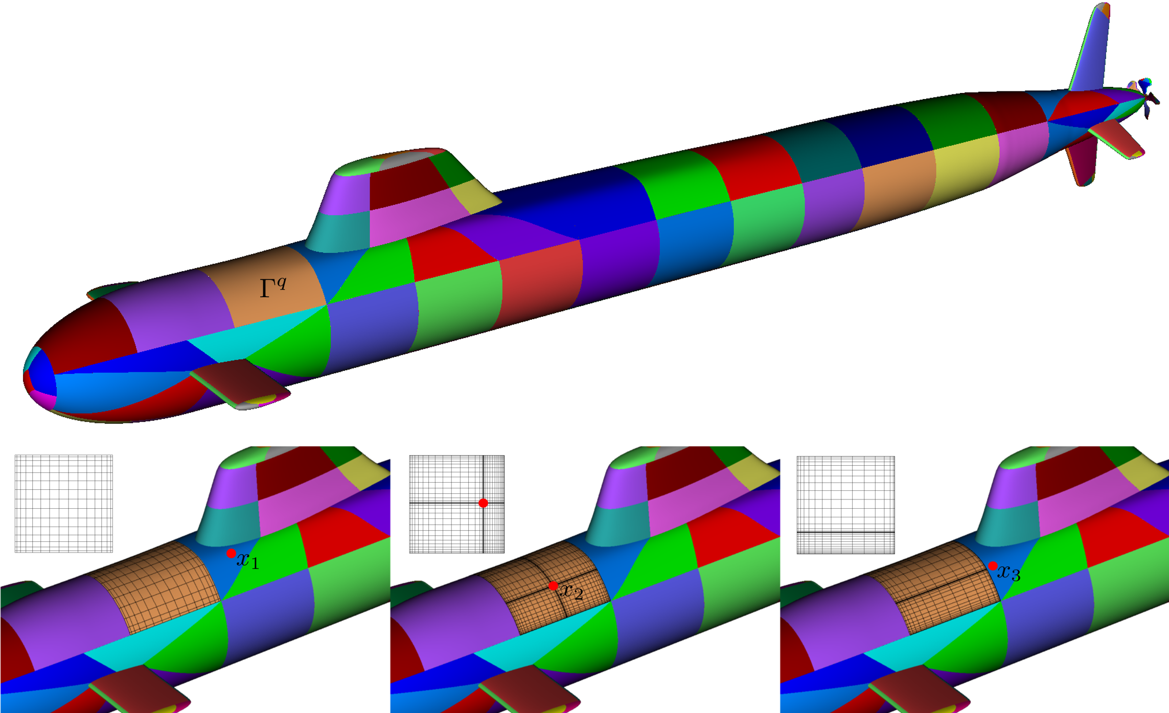
Figure 1: Upper panel: Non-overlapping multi-patch surface representation for a submarine model, with a patch denoted by $\Gamma^{q}$ depicted in light-brown color. Lower left panel: a patch $\Gamma^{q}$ overlaid with a Chebyshev discretization mesh induced by the parameter grid displayed in the leftmost inset parameter patch $(-1,1)^{2}=(-1,1)\times(-1,1)$. An observation point $x_{1}$ far from the patch is shown in red, for which the Fejér first quadrature rule on the aforementioned parameter grid gives rise to accurate integration. Lower center panel: same as the lower-left panel but for an evaluation point $x_{2}$ within the patch $\Gamma^{q}$, and associated graded meshes in the parameter and physical patches. Lower right panel: same as the lower-center panel, for an evaluation point outside but near the patch $\Gamma^{q}$, and associated graded meshes in the parameter and physical patches.

On the basis of such a geometric representation of the surface $\Gamma$, a general surface integral operator

$$\mathcal{I}[\varphi](x)=\int_{\Gamma}K(x,y)\varphi(y)\,dS(y),\quad x\in\Gamma,$$ (12)

such as those in equation (6), can be evaluated in patch-wise fashion,

$$\mathcal{I}[\varphi](x)=\sum_{q=1}^{Q}\mathcal{I}^{q}[\varphi](x)\quad\mbox{where}\quad\mathcal{I}^{q}[\varphi](x)=\int_{\Gamma_{q}}K(x,y)\varphi(y)\,dS(y),\quad x\in\Gamma,$$ (13)

and, thus, the evaluation of $\mathcal{I}[\varphi](x)$ for $x\in\Gamma$ reduces to evaluation of the patch operators $\mathcal{I}^{q}[\varphi](x)$ for all $x\in\Gamma$ and $q=1,\dotsc,Q$. The problem of evaluation of the patch operators $\mathcal{I}^{q}[\varphi](x)$, whose treatment require careful consideration of the position of the point $x\in\Gamma$ relative to the patch $\Gamma_{q}$, is taken up in Section 4.

3 IFGF acceleration of discrete integral operators

As detailed in Section 4, the iterative numerical solution of equation (7) requires evaluation of discrete versions of the integral operators $\mathcal{D}$ and $\mathcal{S}$ introduced in the previous section, for given numerical approximations of the unknown density $\varphi$, on a suitably selected surface mesh $\Gamma_{N}=\{x_{1},\dots,x_{N}\}$, where $x_{j}$ ($1\leq j\leq N$) are pairwise different surface discretization points. Per the discussion in Section 4, the evaluation of such discrete operators entails two main challenges: (a) The accurate evaluation of singular and near-singular contributions (namely, contributions to the integrals in (6) arising from values of $y$ close to a given $x$, for which the singularity of the Green function must be suitably considered); and (b) The efficient evaluation of the vast number of non-singular contributions—which, as discussed in Section 4, reduces to evaluation of discrete operators of the form

$$I_{K}(x_{\ell})=\sum\limits_{\begin{subarray}{c}m=1\\ m\neq\ell\end{subarray}}^{N}a_{m}K(x_{\ell},x_{m}),\quad\ell=1,\ldots,N,$$ (14)

where $a_{m}\in\mathbb{C}$ denote complex numbers, and where $K$ denotes either the Green function itself ($K(x,y)=\Phi(x,y)$) or its normal derivative ($K(x,y)=\frac{\partial\Phi}{\partial\nu(y)}$). The present section addresses the challenges arising from point (b): on the basis of the IFGF recursive interpolation strategy described in Sections 3.1 through 3.3 below, the proposed approach effectively reduces the $\mathcal{O}{(N^{2})}$ cost required by direct evaluation of discrete operators of the form (14) to $\mathcal{O}{(N\log N)}$ operations, in a manner that remains efficiently parallelizable for challenging high-frequency configurations. The IFGF acceleration strategy was introduced for the single layer kernel $K(x,y)=\Phi(x,y)$ in [3] and is extended in in what follows to the double-layer kernel $K(x,y)=\frac{\partial\Phi}{\partial\nu(y)}$.

3.1 Factored Green function: analytic properties

We seek to efficiently evaluate the sum $I_{K}$ in (14) with kernel function $K$ equal to either the single- or double-layer kernel (equations (4) and (5), respectively; cf. (8) and (9)). In the case of the single-layer kernel $\Phi(x,y)=\frac{1}{4\pi}V_{1}(x,y)$ we utilize the factored expression

$$V_{1}(x,y)=\frac{e^{\text{i}kr}}{r}\frac{e^{\text{i}kr\left(\left|\frac{x-y^{0}}{r}-\frac{y-y^{0}}{r}\right|-1\right)}}{\left|\frac{x-y^{0}}{r}-\frac{y-y^{0}}{r}\right|},\quad r=|x-y^{0}|,$$ (15)

which, for points $y$ within a cubic box $B(y^{0},H)$ of side $H$ centered at the point $y^{0}=(y^{0}_{1},y^{0}_{2},y^{0}_{3})$,

$$B(y^{0},H)\coloneqq\bigg{[}y^{0}_{1}-\frac{H}{2},y^{0}_{1}+\frac{H}{2}\bigg{)}\times\bigg{[}y^{0}_{2}-\frac{H}{2},y^{0}_{2}+\frac{H}{2}\bigg{)}\times\bigg{[}y^{0}_{3}-\frac{H}{2},y^{0}_{3}+\frac{H}{2}\bigg{)},$$ (16)

and using a parameter $h$ and a new variable $s$ given by

$$h=\max\limits_{y\in B_{y^{0}}}|y-y^{0}|=\frac{\sqrt{3}}{2}H\quad\mbox{and}\quad s=\frac{h}{r},$$ (17)

we re-express in the form

$$V_{1}(x,y)=\frac{e^{\text{i}kr}}{r}\frac{e^{\text{i}k\frac{h}{s}\left(\left|\frac{x-y^{0}}{r}-\frac{y-y^{0}}{h}s\right|-1\right)}}{\left|\frac{x-y^{0}}{r}-\frac{y-y^{0}}{h}s\right|}=\frac{e^{\text{i}kr}}{r}\widehat{W}_{1}(x,y;y^{0}).$$ (18)

As indicated in what follows, for each fixed $y$, the second factor

$$\widehat{W}_{1}(x,y;y^{0})=\frac{e^{\text{i}k\frac{h}{s}\left(\left|\frac{x-y^{0}}{r}-\frac{y-y^{0}}{h}s\right|-1\right)}}{\left|\frac{x-y^{0}}{r}-\frac{y-y^{0}}{h}s\right|},$$ (19)

can be viewed as an easy-to-interpolate analytic function of $(s,\theta,\varphi)$ around $s=0$ ($r=\infty$), where $\theta$ and $\varphi$ are certain angular variables. In detail, using the “singularity resolving” spherical-coordinate change of variables

$${\mathbf{x}}(s,\theta,\varphi;y^{0})=\tilde{\mathbf{x}}(h/s,\theta,\varphi;y^{0}),$$ (20)

where $\tilde{\mathbf{x}}$ denotes the $y^{0}$-centered classical spherical-coordinate change of variables

$$\tilde{\mathbf{x}}(r,\theta,\phi;y^{0})=y^{0}+\begin{pmatrix}r\sin\theta\cos\phi\\ r\sin\theta\sin\phi\\ r\cos\theta\end{pmatrix},\qquad 0\leq r<\infty,\mkern 5.0mu0\leq\theta\leq\pi,\mkern 5.0mu0\leq\phi<2\pi,$$ (21)

the “analytic factor” $W_{1}(s,\theta,\phi,y;y^{0})$, for $y,y^{0}\in\mathbb{R}^{3}$, is defined by

$$W_{1}(s,\theta,\phi,y;y^{0})=\widehat{W}_{1}(\mathbf{x}(s,\theta,\varphi),y;y^{0})$$ (22)

so that,

$$\mbox{for}\quad x=\mathbf{x}(s,\theta,\varphi;y^{0}),\quad\mbox{we have}\quad\Phi(x,y)=\frac{1}{4\pi}\frac{e^{\text{i}kr}}{r}W_{1}(s,\theta,\phi,y;y^{0}).$$ (23)

Since $\left|\frac{x-y^{0}}{r}\right|=1$, $\frac{y-y^{0}}{h}\leq 1$, the function $W_{1}$ is analytic for all $|s|<1$, including $s=0$ ($r=\infty$). But lines 13 and 18 in Algorithm 1 (presented in Section 3.4 below), show that the IFGF method only interpolates onto points for which $r\geq\frac{3H}{2}$, and, thus, that the IFGF only uses values of $s$ satisfying

$$s=\frac{h}{r}=\frac{\frac{\sqrt{3}H}{2}}{r}\leq\frac{\frac{\sqrt{3}H}{2}}{\frac{3H}{2}}=\frac{\sqrt{3}}{3}\approx 0.577.$$ (24)

In particular, the IFGF application utilizes the function $W_{1}$ well within its domain of analyticity. This function is additionally slowly oscillatory in the $s$ variable [3], cf. Figure 2 and its caption. The function $W_{1}$ may thus be efficiently interpolated in the variables $(s,\theta,\phi)$, with a finite interpolation interval in the $s$ variable accounting for all functional variations up to an including $r=\infty$, by using just a few interpolation intervals in the variable $s$ in conjunction with adequately selected compact interpolation intervals in the $\theta$ and $\phi$ variables, as detailed in Section 3.2. As indicated in that section, following [3], the IFGF method relies on this property to accelerate the evaluation of the sum (14) with kernel $K=\Phi$.

In what follows we seek an analogous factorization for the terms $V_{2}$ and $V_{3}$ in the double-layer expression $\frac{\partial\Phi(x,y)}{\partial\nu(y)}=\frac{1}{4\pi}V_{2}(x,y)-\frac{\text{i}k}{4\pi}V_{3}(x,y)$ displayed in equation (9). Using once again the notations $r=|x-y^{0}|$ and $s=\frac{h}{r}$ we now obtain

$$V_{2}(x,y) =\frac{e^{\text{i}kr}}{r^{2}}\frac{e^{\text{i}k\frac{h}{s}\left(\left|\frac{x-y^{0}}{r}-\frac{y-y^{0}}{h}s\right|-1\right)}}{\left|\frac{x-y^{0}}{r}-\frac{y-y^{0}}{h}s\right|^{3}}\left\langle\frac{x-y^{0}}{r}-\frac{y-y^{0}}{h}s,\nu(y)\right\rangle=\frac{e^{\text{i}kr}}{r^{2}}\widehat{W}_{2}(x,y;y^{0}),$$ (25a)

$$V_{3}(x,y) =\frac{e^{\text{i}kr}}{r}\frac{e^{\text{i}k\frac{h}{s}\left(\left|\frac{x-y^{0}}{r}-\frac{y-y^{0}}{h}s\right|-1\right)}}{\left|\frac{x-y^{0}}{r}-\frac{y-y^{0}}{h}s\right|^{2}}\left\langle\frac{x-y^{0}}{r}-\frac{y-y^{0}}{h}s,\nu(y)\right\rangle=\frac{e^{\text{i}kr}}{r}\widehat{W}_{3}(x,y;y^{0}),$$ (25b)

where

$$\widehat{W}_{2}(x,y;y^{0}) =\frac{e^{\text{i}k\frac{h}{s}\left(\left|\frac{x-y^{0}}{r}-\frac{y-y^{0}}{h}s\right|-1\right)}}{\left|\frac{x-y^{0}}{r}-\frac{y-y^{0}}{h}s\right|^{3}}\left\langle\frac{x-y^{0}}{r}-\frac{y-y^{0}}{h}s,\nu(y)\right\rangle$$ (26a)

$$\widehat{W}_{3}(x,y;y^{0}) =\frac{e^{\text{i}k\frac{h}{s}\left(\left|\frac{x-y^{0}}{r}-\frac{y-y^{0}}{h}s\right|-1\right)}}{\left|\frac{x-y^{0}}{r}-\frac{y-y^{0}}{h}s\right|^{2}}\left\langle\frac{x-y^{0}}{r}-\frac{y-y^{0}}{h}s,\nu(y)\right\rangle.$$ (26b)

Defining, for $y^{0}\in\mathbb{R}^{3}$ and $y\in B(y^{0},H)$, the analytic factors

$$W_{2}(s,\theta,\phi,y;y^{0})=\widehat{W}_{2}({\mathbf{x}(s,\theta,\varphi),y;y^{0})}\quad\mbox{and}\quad W_{3}(s,\theta,\phi,y;y^{0})=\widehat{W}_{3}({\mathbf{x}(s,\theta,\varphi),y;y^{0})}$$ (27)

the relations (cf. (22)),

$$\mbox{for}\quad x=\mathbf{x}(s,\theta,\varphi;y^{0}),\quad\frac{\partial\Phi(x,y)}{\partial\nu(y)}=\frac{1}{4\pi}\frac{e^{\text{i}kr}}{r^{2}}W_{2}(s,\theta,\phi,y;y^{0})-\text{i}k\frac{1}{4\pi}\frac{e^{\text{i}kr}}{r}W_{3}(s,\theta,\phi,y;y^{0})$$ (28)

follow. Clearly, like the analytic factor $W_{1}$ in equation (22), $W_{2}$ and $W_{3}$ are analytic functions of $s$ for all $|s|<1$. Thus, per equation (24) and associated parenthetical comment, these functions can be effectively interpolated in the IFGF context using a small number of interpolation intervals in the variable $s$ in conjunction with adequately selected interpolation intervals in the $\theta$ and $\phi$ variables, as detailed in Section 3.2.

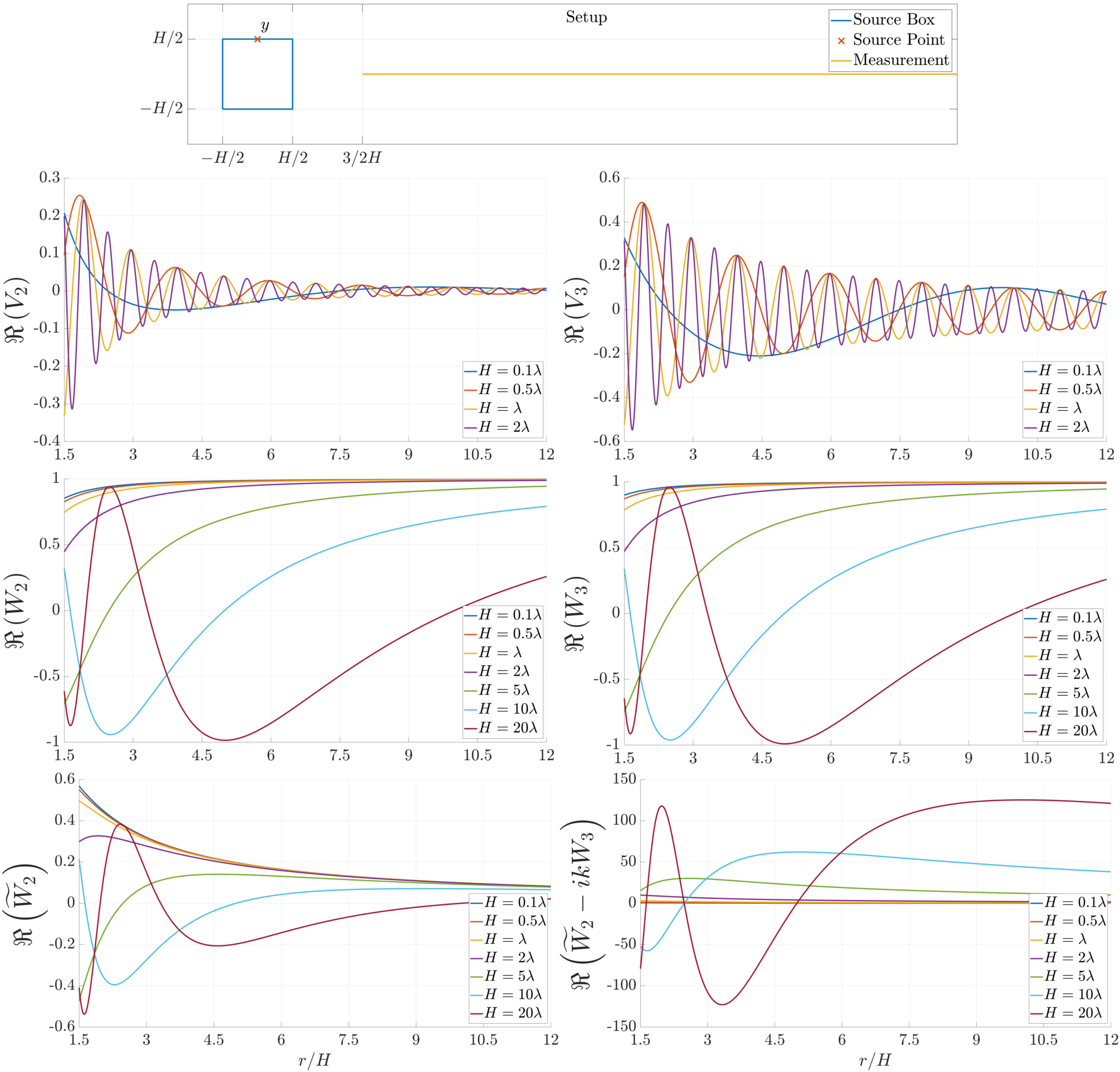
Figure 2: Source-point factorization test, set up as illustrated in the “Setup” panel. The subsequent two panels demonstrate the highly oscillatory character of the double-layer kernel components $V_{2}$ and $V_{3}$ (the graphs display the real parts $\Re(V_{2})$ and $\Re(V_{3})$ of $V_{2}$ and $V_{3}$), even for small values of $H$ ($H\leq 2\lambda$). The final four panels illustrate the corresponding slowly oscillatory character of various IFGF analytic factors introduced in Section 3.1, for $H$ values up to $H=20\lambda$. The factor $W_{1}$, which is considered in [3], and which is quite similar in form and character to $W_{3}$, is not included in this figure, for conciseness.

It is important to note here that, in many cases, it is more efficient to evaluate double-layer potential contributions via interpolation of the single function

$$W_{4}=\widetilde{W}_{2}-\text{i}kW_{3},\quad\mbox{where}\quad\widetilde{W}_{2}=\widetilde{W}_{2}(s,\theta,\phi,y;y^{0})=\frac{1}{r}W_{2}(s,\theta,\phi,y;y^{0})=\frac{s}{h}W_{2}(s,\theta,\phi,y;y^{0}),$$ (29)

instead of separately interpolating each of the two functions $W_{2}$ and $W_{3}$ (as required when using the decomposition (28)), thereby leading to an IFGF cost reduction by a factor of two. Indeed, paralleling the decompositions (22) and (28), in this case we obtain the expression

$$\frac{\partial\Phi(x,y)}{\partial\nu(y)}=\frac{1}{4\pi}\frac{e^{\text{i}kr}}{r}\left(\widetilde{W}_{2}(s,\theta,\phi,y;y^{0})-\text{i}kW_{3}(s,\theta,\phi,y;y^{0})\right)=\frac{1}{4\pi}\frac{e^{\text{i}kr}}{r}W_{4}(s,\theta,\phi,y;y^{0})$$ (30)

in terms of the single function $W_{4}$. Like the previously considered functions $W_{1}$, $W_{2}$ and $W_{3}$, the function $W_{4}$ is also an analytic function of $s$ for $|s|<1$. As discussed in Section 3.3, interpolation of the function $W_{4}$ can lead to larger errors in the resulting values of $\frac{\partial\Phi(x,y)}{\partial\nu(y)}$, for small values of $h$, but its use is advantageous for values of $h$ bounded away from zero.

The oscillatory character of the various analytic factors is illustrated in Figure 2—omitting, for brevity, the factor $W_{1}$, which is considered in [3], and which is quite similar in form and character to $W_{3}$. For clarity, for these examples the cube side $H$ is used as a measure of the size of the interpolation problem instead of the parameter $h=\frac{\sqrt{3}}{2}H$. The test setup is laid down at the top of Figure 2. It shows a single source point at the position $y$ that, as it happens, gives rise to the fastest possible oscillations along the measurement line (shown as a solid yellow line) among all possible source positions at and within the blue source box. Panels (a) and (b) demonstrate the highly oscillatory character of the double-layer kernel components $V_{2}$ and $V_{3}$, even for small values of $H$ ($H\leq 2\lambda$); the component $V_{1}$ exhibits a similar oscillatory character. Panels (c)-(f), in turn, illustrate the corresponding slowly oscillatory character of various IFGF analytic factors introduced in the present section, even for much larger values of $H$—e.g., for $H$ values up to $H=20\lambda$. Clearly, the analytic factors $W_{j}$, $j=1,\dotsc,4$, oscillate much more slowly than the corresponding full kernel components $V_{j}$, and, as expected from the discussion above in this section, they actually tend to a finite limit as $r\to\infty$. All of these functions can therefore be interpolated more effectively than the corresponding functions $V_{j}$. As indicated above, however, a key difference in the analytic factor $\widetilde{W}_{2}$ (and, thus, $W_{4}$), which is not noticeable in this figure, becomes apparent as the problem of interpolation is considered—as discussed in the following section and highlighted in Figure 3.

3.2 Factored Green function: single-box interpolation

To appropriately structure an interpolation approach that takes advantage of the slowly oscillatory character of the analytic factors introduced in the previous section, we consider the $y^{0}$-centered axes-aligned cubic box $B(y^{0},H)$ of side $H$ and centered at $y^{0}$. As discussed in what follows, for all target points $x_{\ell}$ that are at least one box away from $B(y^{0},H)$, the sum of all contributions arising from the sources contained in $B(y^{0},H)\cap\Gamma_{N}$ can be effectively evaluated via interpolation of the corresponding analytic factors $W_{j}$, $j=1,\dotsc,4$—since, for such target points we have $(r,\theta,\phi)\in\mathcal{E}\coloneqq[3H/2,\infty]\times[0,\pi]\times[0,2\pi)$ or, equivalently, $(s,\theta,\phi)\in[0,\eta]\times[0,\pi]\times[0,2\pi)$, where $\eta=\sqrt{3}/3$.

To tackle the interpolation task, the target domain $\mathcal{E}$ is partitioned as described in what follows. Letting, for given positive integers $n_{s}$ and $n_{C}$,

$$\Delta s=\frac{\eta}{n_{s}}\quad\text{ and }\quad\Delta\theta=\Delta\phi=\frac{\pi}{n_{C}},$$ (31)

and $K_{C}\coloneqq\{1,\dotsc,n_{s}\}\times\{1,\dotsc,n_{C}\}\times\{1,\dotsc,2n_{C}\}$, and letting, for each $\boldsymbol{\gamma}=(\gamma_{1},\gamma_{2},\gamma_{3})\in K_{C}$, $s_{\gamma_{1}}=\gamma_{1}\Delta s$, $\theta_{\gamma_{2}}=\gamma_{2}\Delta\theta$ and $\phi_{\gamma_{3}}=\gamma_{3}\Delta\phi$, interpolation intervals $E^{s}_{\gamma_{1}},\,E^{\theta}_{\gamma_{2},\gamma_{3}}$ and $E^{\phi}_{\gamma_{3}}$ along the $s,\,\theta,$ and $\phi$ directions are defined by

$$E^{s}_{\gamma_{1}}=[s_{\gamma_{1}-1},s_{\gamma_{1}}),\qquad E^{\theta}_{\gamma_{2},\gamma_{3}}=\begin{cases}[\theta_{n_{C}-1},\pi]&\text{for }\gamma_{2}=n_{C},\,\gamma_{3}=2n_{C}\\ (0,\Delta\theta)&\text{for }\gamma_{2}=1,\,\gamma_{3}>1\\ [\theta_{\gamma_{2}-1},\theta_{\gamma_{2}})&\text{otherwise,}\end{cases}\qquad E^{\phi}_{\gamma_{3}}=[\phi_{\gamma_{3}-1},\phi_{\gamma_{3}}).$$ (32)

For each $\boldsymbol{\gamma}=(\gamma_{1},\gamma_{2},\gamma_{3})\in K_{C}$, we call

$$E_{\boldsymbol{\gamma}}\coloneqq E^{s}_{\gamma_{1}}\times E^{\theta}_{\gamma_{2},\gamma_{3}}\times E^{\phi}_{\gamma_{3}}$$ (33)

a cone domain, and the image of $E_{\boldsymbol{\gamma}}$ under the parametrization (20),

$$C_{\boldsymbol{\gamma}}(y^{0})\coloneqq\left\{x=\mathbf{x}(s,\theta,\phi;y^{0})\,:\,(s,\theta,\phi)\in E_{\boldsymbol{\gamma}}\right\},$$ (34)

a cone segment. Note that

$$\mathcal{E}=\bigcup\limits_{\boldsymbol{\gamma}\in K_{C}}C_{\boldsymbol{\gamma}}(y^{0})\quad\text{ and }\quad C_{\boldsymbol{\gamma}}(y^{0})\cap C_{\boldsymbol{\gamma}^{\prime}}(y^{0})=\varnothing\quad\text{ for }\boldsymbol{\gamma}\neq\boldsymbol{\gamma}^{\prime}.$$

Remark 1.

The recursive interpolation method introduced in the following section, which utilizes boxes $B(y^{0},H)$ of various sizes $H$ and for various centers $y^{0}$, requires, for each box size $H$ used, selection of numbers $n_{s}=n_{s}(H)$ and $n_{C}=n_{C}(H)$ in equation (31) which ensure cone-segment interpolation at essentially constant accuracy for all used values of $H$. Such selection is facilitated by Theorems 1 and 2 in [3], which relate the acoustic size $kH$ of the box $B(y^{0},H)$ to the error arising from cone-segment interpolation. In particular, these theorems imply that fixed numbers $n_{s}$ and $n_{C}$ give rise to essentially constant cone-segment interpolation errors for all $H$-side boxes satisfying $kH<1$. Additionally, these results tell us that, for box sizes in the complementary $kH\geq 1$ case, doubling the box size $H$ requires doubling the numbers $n_{s}$ and $n_{C}$ (resulting in a two-fold refinement of cone segments in each of the three spherical-coordinate directions) in order to ensure an essentially unchanging cone-segment interpolation error. Accordingly, given integer initial values $n_{C,0}\geq 1$ and $n_{S,0}\geq 1$, the IFGF algorithm uses constant values $n_{C}=n_{C,0}$ and $n_{s}=n_{S,0}$ for all box sizes $H$ satisfying $kH\leq 1/2$, and, then, for box sizes $H$ for which $kH>1/2$, the algorithm doubles the numbers $n_{s}$ and $n_{C}$ as it transitions from a level $d$ (with, say, box size $H$) to a subsequent level $(d-1)$ (with box size $2H$). Throughout this paper the box sizes at the initial level $d=D$ were taken to satisfy the condition $kH<1$, and the selections $n_{C,0}=2$ and $n_{S,0}=1$ were used. Note that, for such values, at levels $d$ for which $kH\leq 1/2$, if any such levels exist, each box $B(y^{0},H)$ is furnished with a total of eight cone segments, each one an unbounded octant section ranging from $r=\frac{3H}{2}$ ($s=\frac{\sqrt{3}}{3}$) to $r=\infty$ ($s=0$). Such a coarse cone-segment partition used in conjunction with polynomial interpolation by a single polynomial in each conical-segment coordinate variable, as described in what follows, with polynomial degrees such as, e.g., degree 3 in the radial variable $s$, and degree 5 in the angular variables $\theta$ and $\phi$, suffices to provide accuracies of the orders demonstrated in Section 5.

The proposed 3D interpolation strategy within cone segments $C_{\boldsymbol{\gamma}}$ amounts to a tensor product of 1D Chebyshev interpolation schemes based on use of fixed numbers $P_{s}$ and $P_{\rm{ang}}$ of interpolation points along the radial and angular variables, respectively, for a total of $P=P_{s}P^{2}_{\rm{ang}}$ interpolation points in each cone segment $C_{\boldsymbol{\gamma}}$. The underlying 1D Chebyshev interpolating scheme is defined, for a given function $u:[-1,1]\to\mathbb{C}$, as the interpolating polynomial $I_{n}u$ of degree $(n-1)$ given by

$$I_{n}u(x)=\sum_{i=0}^{n-1}a_{i}T_{i}(x),\qquad x\in[-1,1],$$ (35)

where $T_{i}(x)=\cos(i\arccos(x))$. The coefficients $a_{i}$ are given by

$$a_{i}=\frac{2}{b_{i}(n-1)}\sum_{k=0}^{n-1}c_{k}u(x_{k})T_{i}(x_{k}),$$ (36)

where, for $i=0,\dotsc,n-1$,

$$x_{k}=\cos\left(\frac{2k+1}{2n}\pi\right),\quad b_{i}=\begin{cases}1&i\neq 0\\ 2&i=0,\end{cases}\quad c_{k}=\begin{cases}0.5&k=0\text{ or }k=n-1\\ 1&\text{otherwise}.\end{cases}$$ (37)

Use of the spherical-coordinate Chebyshev interpolation approach associated with the box $B(y^{0},H)$ can be applied to obtain approximate values of each one of the analytic factors $W_{j}(s,\theta,\phi,y;y^{0})$, $j=1,\dotsc,4$ defined in Section 3.1, for any given source point $y\in B(y^{0},H)$ and any given target point $x=\mathbf{x}(s,\theta,\phi)$ (with $y^{0}$-centered spherical coordinates $(s,\theta,\phi)$) that is at least one size-$H$ box away from $B(y^{0},H)$. By linearity, the same interpolation method can be applied, with similar accuracy, to linear combinations such as the one given by the sum over $y$ on the right-hand side of the relation

$$S^{H,y^{0}}_{j}(s,\theta,\phi)=\frac{e^{\text{i}k|x-y^{0}|}}{4\pi|x-y^{0}|^{q_{j}}}\sum\limits_{y\in B(y^{0},H)\cap\Gamma_{N}}a(y)W_{j}(s,\theta,\phi,y;y^{0}),$$ (38)

for any given number of sources within the box $B(y^{0},H)$ and for given coefficients $a(y)$. Here, with reference to the factorizations introduced in Section 3.1, we have set $q_{2}=2$ and $q_{j}=1$ for $j=1,3,4$.

In view of the factorizations displayed in (23) and (28), interpolation of the sum over $y$ in (38) with $j=1,2,3$ can be used to accelerate the evaluation of the sum (14) with $K$ equal to either the single-layer or the double-layer kernels (4) and (5). As discussed in the following section, however, in the case of the double-layer kernel a more efficient interpolation strategy can be devised by utilizing, in addition, the factorization (30) associated with the analytic factor $W_{4}$.

3.3 IFGF method for the double-layer potential

In order to study the relative advantages offered by the interpolation strategies arising from the concepts introduced in Sections 3.1 and 3.2, we consider Figure 3, which displays absolute errors in IFGF approximations associated with the single- and double-layer potentials. For this experiment, single- and double-layer potentials resulting from a total of 200 source points on a spherical surface contained within the box $B(y^{0},H)$ were considered, as depicted in the figure inset, and errors along the radial line shown in the inset were evaluated and are displayed in the figure. Only radial interpolations were performed, since the angular factorizations are identical for all the factored forms used. The various error curves, labeled SL, DL and $\widetilde{DL}$ in the figure, display absolute errors arising in the approximation of the single- and double-layer potentials, namely, the error SL in the single-layer approximation resulting from use of the factorization (23), and the errors DL and $\widetilde{DL}$ in the double-layer approximations resulting from use of the factorizations (28) and (30), respectively. Mirroring the octree IFGF structure described in the following section, abscissae for the points in the graph are given by powers of $2$ times a fixed constant. In each case the error resulting from interpolation of analytic factors was computed over a single interpolation interval, namely, the interpolation interval starting at a distance $H$ from the source box—the closest interval to the source box, and, therefore, the one giving rise to the largest interpolation errors. In accordance with Remark 1, for $kH<1$, the interval spans the complete semi-infinite line (i.e., the complete interval $0\leq s\leq\frac{\sqrt{3}}{3})$), and, starting from $kH=\pi$ (that is, $H/\lambda=0.5$, which is marked by a vertical dashed line in the figure) the interval size in the $s$ variable is halved every time $kH$ is doubled. Interpolations were performed using a total of $P_{s}=3$ interpolation points along the interval, and IFGF errors were evaluated at $200$ equispaced target test points in the interval. Clearly, over wide $H/\lambda$ ranges, spanning from $H/\lambda=0.5$ all the way to $H/\lambda=\infty$, the interpolation scheme associated with the factorization $\widetilde{DL}$, which requires interpolation of the single analytic factor $W_{4}$, incurs the same error as the more expensive scheme arising from interpolation of the decomposition DL—which requires interpolation of the two analytic factors $W_{2}$ and $W_{3}$. The curve indicates, however, that the $\widetilde{DL}$ scheme does lead to significant accuracy losses versus the DL scheme, when used for $H/\lambda<0.5$. The increased error displayed by the $\widetilde{DL}$ curve in the range $H/\lambda<0.5$ can be traced to the partial factorization of the $\frac{1}{r}$ term associated with the analytic factor $\widetilde{W}_{2}$ (which still contains a singular component, as evidenced by the $1/r$ term in equation (29)), versus the fully regularized decomposition (28). The right-hand expression in equation (29) provides a different perspective on the phenomenology, as it shows that the $\widetilde{DL}$ factorization suffers from increased errors for small values of $h$, and thus, in view of (17), for small values of $H/\lambda$.

While rigorously accounting for the Green function singularity and maintaining accuracy for arbitrarily small values of the source box size $H/\lambda$, the approach demonstrated in the DL curves, which is based on interpolation of the analytic factors $W_{2}$ and $W_{3}$, doubles the cost of the IFGF accelerator vis-à-vis the $W_{4}$-based method associated with the $\widetilde{DL}$ curves. An optimal strategy then calls for use of the $W_{2}$-$W_{3}$ based method for the portion of the IFGF octree containing boxes of size $H/\lambda<0.5\lambda$, and use of the $W_{4}$-based method for the remainder the octree. For the structures considered in this paper, most of which do not contain significant subwavelength geometric features, the second approach is advantageous throughout the complete IFGF octree—as it enjoys the reduced computational cost while preserving accuracy. In a more general context a hybrid $W_{2}$-$W_{3}$/$W_{4}$ approach as described above would be used which, additionally, would incorporate adaptivity in the box sizes in regions containing finely meshed surfaces (as discussed in Section 5.3 in connection with the submarine propeller structure). Such extensions are beyond the scope of this paper, and are left for future work.

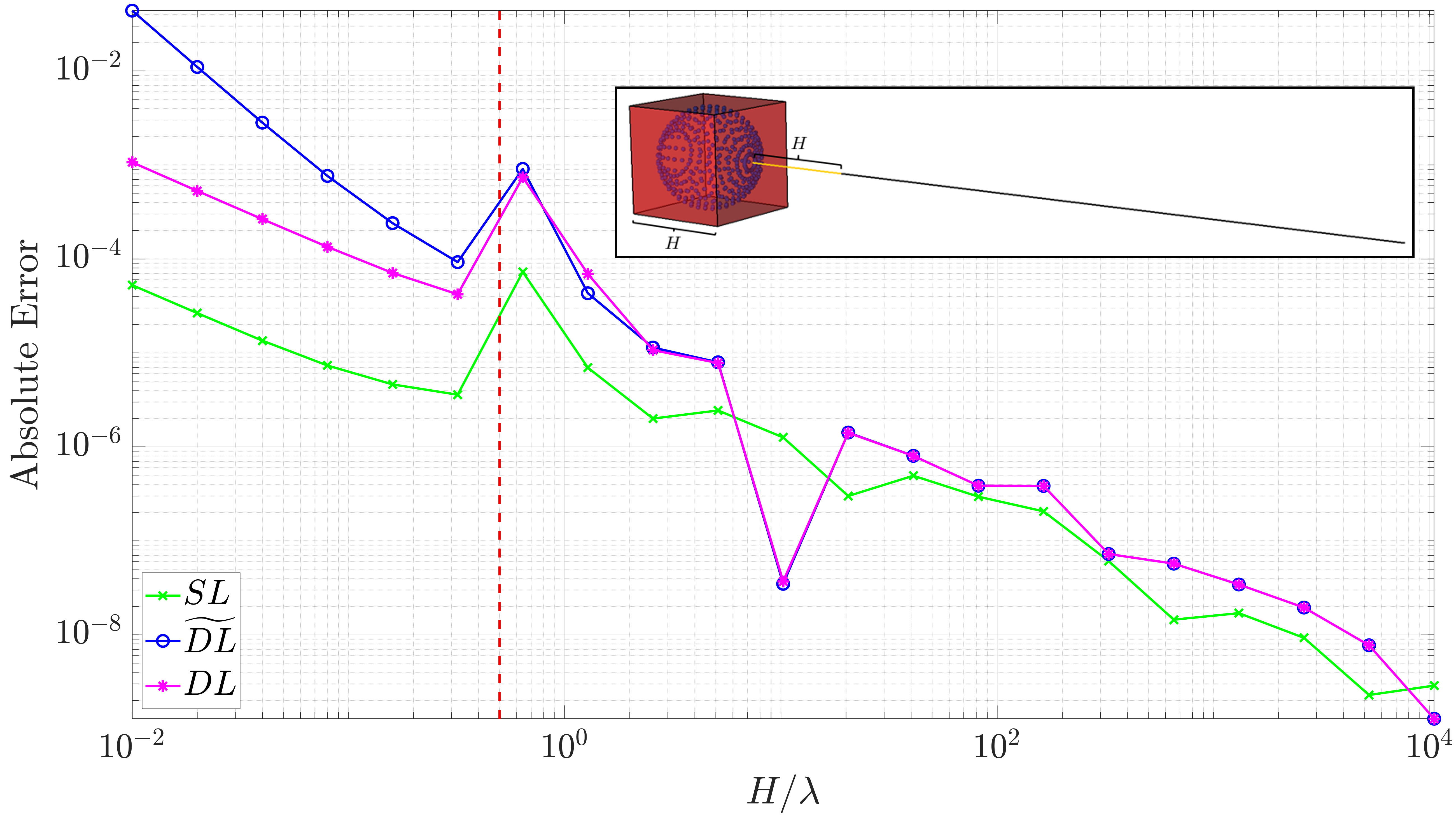
Figure 3: Maximum absolute errors arising in IFGF representation of the single-layer and double-layer potentials. In the configuration considered for this test, 200 sources $y\in\Gamma\subset B(y^{0},H)$, located on the spherical surface $\Gamma$ and contained in the box $B(y^{0},H)$, were used, as shown in the inset. The curves presented illustrate the character of three IFGF-interpolation algorithms, namely, 1) Interpolation of the single-layer potential on the basis of (23) by means of (38) with $j=1$ (curve labeled “$SL$”, shown in green); 2) Interpolation of the double-layer potential on the basis of equation (30) by means of (38) with $j=4$ (curve labeled “$\widetilde{DL}$”, shown in blue), and 3) Interpolation of the double-layer potential on the basis of equation (28) by means of a combination of the $j=2$ and $j=3$ versions of (38) (curve labeled “$DL$”, shown in magenta). The errors shown were evaluated as the maximum of the errors obtained at a set of 200 target points $x=\mathbf{x}(s,\theta,\varphi;y^{0})$, with $\theta=\varphi=0$, located at a distance greater than or equal to $H$ from the boundary of $B$ along a radial line exterior to $B$, as shown in the inset. Clearly the $\widetilde{DL}$ and $DL$ errors essentially coincide to the right of the line $H/\lambda=0.5$ (vertical dashed red line)—, which, as discussed in Section 3.3, enables certain efficiency gains in the evaluation of double-layer potentials.

3.4 Factored Green function: recursive interpolation

To effect the desired evaluation of discrete operators (14) at $\mathcal{O}(N\log N)$ computing cost, the IFGF approach implements the interpolation scheme described in Sections 3.1 through 3.3 in a recursive manner, in sets of larger and larger boxes, so that the values required by the interpolation scheme associated with a large box can themselves be obtained by interpolation from smaller boxes. The IFGF method implements such a recursive interpolation scheme on the basis of a $D$-level octree sequence of partitions of the discrete surface $\Gamma_{N}$ [3] for a suitably selected $D\in\mathbb{N}$. Thus, the boxes are defined iteratively starting from the single level $d=1$ box $B_{(1,1,1)}^{1}\supset\Gamma_{N}$, leading to the trivial partition of $\Gamma_{N}$ into a single subset equal to all of $\Gamma_{N}$. For $d=2,\dotsc,D$, in turn, the level-$d$ boxes are defined via partition of each of the level $(d-1)$ boxes into eight equi-sized and disjoint boxes of side $H_{d}=H_{d-1}/2$, resulting in the level $d$ boxes $B^{d}_{\mathbf{k}}=B(y^{\mathbf{k}}_{d},H_{d})\subset\mathbb{R}^{3}$ (see equation (16)), for $\mathbf{k}\in I^{d}_{B}\coloneqq\{1,\ldots,2^{d-1}\}^{3}$, and for certain box centers $y^{\mathbf{k}}_{d}$. Clearly, each box $B^{d}_{\mathbf{k}}$ on level $d$ ($2\leq d\leq D$) is contained in a parent box on level $d-1$, which we denote by $\mathcal{P}B^{d}_{\mathbf{k}}$. The level-$d$ partition of $\Gamma_{N}$ is obtained via intersection of $\Gamma_{N}$ with each one of the level-$d$ boxes. Figure 4(a) illustrates an analogous two-dimensional hierarchical quadtree structure in the $D=3$ (three-level) case.

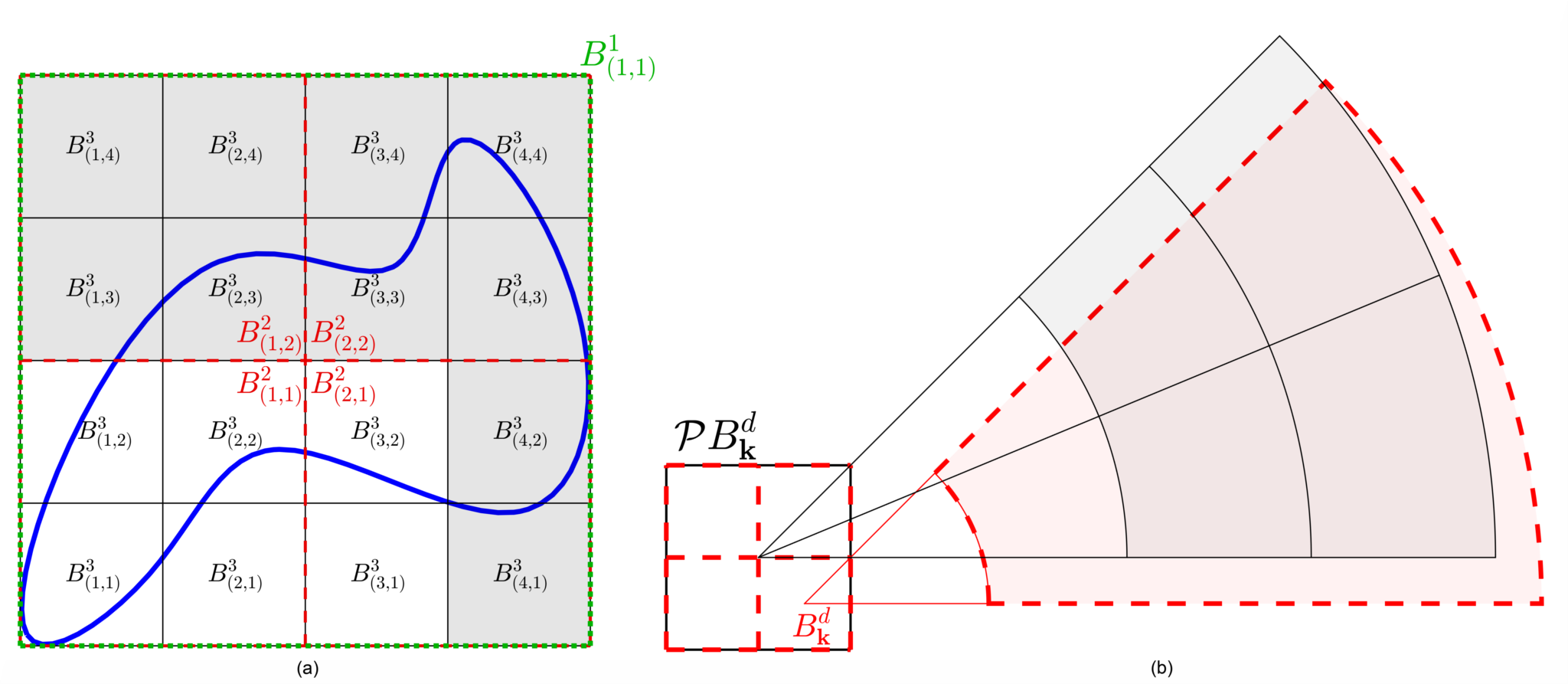
Figure 4: (a) Two-dimensional sketch of the IFGF domain decomposition for the three-level $(D=3)$ case, with a scatterer is sketched in blue. In particular, the figure displays the neighbors (white boxes) and cousins (gray boxes) of the box $B_{(2,1)}^{3}$. (b) Illustration of typical cone segments for a box $B_{\mathbf{k}}^{d}$ (shown in red and centered at the southeast red box) and its parent box with some associated cone segments (drawn in black).

On the basis of these concepts we utilize the functions $S^{H,y^{0}}_{j}(s,\theta,\phi)$ in (38) with $y^{0}=y^{\mathbf{k}}_{d}$ and $H=H_{d}$ (and, thus, with $B(y^{0},H)=B^{d}_{\mathbf{k}}$), which in what follows are denoted by

$$S^{\mathbf{k},d}_{j}(s,\theta,\phi)=S^{H_{d},y^{\mathbf{k}}_{d}}_{j}(s,\theta,\phi)=\frac{e^{\text{i}kr_{\mathbf{k}}}}{4\pi r_{\mathbf{k}}^{q_{j}}}F^{\mathbf{k},d}_{j}(s,\theta,\phi),$$ (39)

where $a(y)$ are given coefficients, where $r_{\mathbf{k}}\coloneqq|\mathbf{x}(s,\theta,\varphi;y^{\mathbf{k}}_{d})-y^{\mathbf{k}}_{d}|$, and where,

$$\mbox{letting}\quad W^{\mathbf{k},d}_{j}(s,\theta,\phi,y)=W_{j}(s,\theta,\phi,y;y^{\mathbf{k}}_{d}),\quad\mbox{we have set}\quad F^{\mathbf{k},d}_{j}(s,\theta,\phi)=\sum\limits_{y\in B_{\mathbf{k}}^{d}\cap\Gamma_{N}}a(y)W^{\mathbf{k},d}_{j}(s,\theta,\phi,y).$$ (40)

As discussed below in this section, the proposed recursive interpolation approach relies on application of the single-box interpolation strategy described in Sections 3.1 through 3.3 to each one the source boxes $B^{d}_{\mathbf{k}}=B(y^{\mathbf{k}}_{d},H_{d})$ and factors $F^{\mathbf{k},d}_{j}$, starting at level $d=D$ and then proceeding to levels $d=D-1,...$ until all relevant levels $d=D,\dotsc,3$ have been tackled. (The algorithm indeed stops at level $d=3$ since, per construction of the boxes and definition of cousins, at that stage all boxes are cousins and therefore, at the end of that stage all interactions have already been taken into account.)

Clearly, it is only necessary to effect interpolations for relevant boxes $B_{\mathbf{k}}^{d}$, namely, boxes $B_{\mathbf{k}}^{d}$ that contain at least one surface discretization point; the set $\mathcal{R}_{B}$ of all relevant boxes, including boxes at any level $d$ ($1\leq d\leq D$), is denoted by

$$\mathcal{R}_{B}:=\left\{B^{d}_{\mathbf{k}}\,:\,\Gamma_{N}\cap B_{\mathbf{k}}^{d}\neq\varnothing,\,1\leq d\leq D,\,\mathbf{k}\in I^{d}_{B}\right\}.$$ (41)

To facilitate the discussion, several additional but related concepts are introduced, including, for a given level-$d$ box $B^{d}_{\mathbf{k}}$, the set $\mathcal{N}B^{d}_{\mathbf{k}}$ of all level-$d$ boxes that are neighbors of $B^{d}_{\mathbf{k}}$, and the set $\mathcal{M}B^{d}_{\mathbf{k}}$ of all level-$d$ boxes that are cousins of $B^{d}_{\mathbf{k}}$ (that is to say, non-neighboring boxes who are children of the parents’ neighbors). The sets $\mathcal{U}B^{d}_{\mathbf{k}}$ and $\mathcal{V}B^{d}_{\mathbf{k}}$ of neighbor points and cousin points of $B^{d}_{\mathbf{k}}$, respectively, are defined as the set all points in $\Gamma_{N}$ that are contained in neighbor and cousin boxes of $B^{d}_{\mathbf{k}}$, respectively. We clearly have

$$\mathcal{N}B^{d}_{\mathbf{k}} :=\{B_{\mathbf{j}}^{d}\in\mathcal{R}_{B}:||\mathbf{j}-\mathbf{k}||_{\infty}\leq 1\},$$ (42a)

$$\mathcal{M}B^{d}_{\mathbf{k}} :=\{B_{\mathbf{j}}^{d}\in\mathcal{R}_{B}:B_{\mathbf{j}}^{d}\notin\mathcal{N}B_{\mathbf{k}}^{d}\wedge\mathcal{P}B_{\mathbf{j}}^{d}\in\mathcal{N}\mathcal{P}B_{\mathbf{k}}^{d}\}$$ (42b)

$$\mathcal{U}B^{d}_{\mathbf{k}} :=\left(\bigcup\limits_{B\in\mathcal{N}B_{\mathbf{k}}^{d}}B\right)\cap\Gamma_{N}$$ (42c)

$$\mathcal{V}B^{d}_{\mathbf{k}} :=\left(\bigcup\limits_{B\in\mathcal{M}B_{\mathbf{k}}^{d}}B\right)\cap\Gamma_{N}.$$ (42d)

Figure 4(a) presents, in a two-dimensional setting, the neighbor and cousin boxes (shown in white and gray, respectively) of the box $B_{(2,1)}^{3}$.

The IFGF algorithm accelerates the evaluation of (14) by incrementally incorporating pairwise interactions of level-$d$ cousin boxes, for $d=D,\ldots,3$: at stage $d$ the algorithm evaluates, by cone-segment spherical-coordinate interpolation, contributions from each level-$d$ box $B^{d}_{\mathbf{k}}$ to all surface discretization points that lie on cousin boxes of $B^{d}_{\mathbf{k}}$, as well as all cone-segment interpolation points necessary at the subsequent level $(d-1)$ of the interpolation scheme. Note that when level $d$ is reached, values of fields resulting from sources within $B^{d}_{\mathbf{k}}$ at points in boxes neighboring $B^{d}_{\mathbf{k}}$ have already been computed at the previously treated levels $D,D-1,\dotsc,d+1$ (but see Remark 2 below). Once the level-$d$ interpolations have been performed at all necessary cousin points and level-$(d-1)$ interpolation points associated with the box $B^{d}_{\mathbf{k}}$, the complete result $S^{\mathbf{k},d}_{j}(s,\theta,\phi)$ for that box at each required cousin and interpolation point is obtained by multiplication of the interpolated values $F^{\mathbf{k},d}_{j}(s,\theta,\phi)$ with the corresponding value of the “centered factor”

$$E^{\mathbf{k},d}_{j}(s,\theta,\phi)=\frac{e^{\text{i}kr_{\mathbf{k}}}}{4\pi r_{\mathbf{k}}^{q_{j}}}.$$ (43)

Remark 2.

An exception to the interpolation-based method just described occurs at the finest (initial) level $d=D$, for which there are no preceding levels, and for which fields at boxes neighboring $B_{\mathbf{k}}^{D}$ have therefore not been previously obtained. Thus, at level $d=D$, interactions from source points $B_{\mathbf{k}}^{D}$ to points in neighboring boxes are not evaluated by means of an interpolation scheme. Instead, in the context of this section, in which the values of the sum (14) are to be produced, such interactions are obtained via direct summation of the corresponding $B_{\mathbf{k}}^{D}$ contributions. In other contexts, in which the IFGF is used as part of an integration scheme (such as the one introduced in Section 4), certain nearby interactions need to be handled by specialized quadrature rules (such as the ones introduced in Section 4.2) while others do proceed via direct summation.

As suggested above, the IFGF method evaluates the necessary cousin interactions for a single- and double-layer kernels by means of simple piecewise interpolation of the relevant factor(s) $F^{\mathbf{k},d}_{j}(s,\theta,\phi)$ ($j=1,\dots,4$). Per the discussion in Sections 3.1 through 3.3, the interpolations associated with a level-$d$ relevant box $B^{d}_{\mathbf{k}}$ ($\mathbf{k}\in I_{B}^{d}$) are effected by relying on level-$d$ cone segments, which in what follows are denoted by

$$C_{\mathbf{k};\boldsymbol{\gamma}}^{d}=C_{\boldsymbol{\gamma}}(y^{\mathbf{k}}_{d}),\quad\boldsymbol{\gamma}\in K_{C}^{d},\,\mathbf{k}\in I^{d}_{B}$$

(cf. (34)), where, for certain selections of integers $n_{s}=n^{d}_{s}$ and $n_{C}=n^{d}_{C}$, we have used the index set $K_{C}^{d}=\{1,\dotsc,n^{d}_{s}\}\times\{1,\dotsc,n^{d}_{C}\}\times\{1,\dotsc,2n^{d}_{C}\}$, resulting in radial and angular interpolation intervals of lengths $\Delta s=\frac{\eta}{n^{d}_{s}}$ and $\Delta\theta=\Delta\phi=\frac{\pi}{n^{d}_{C}}$ (cf. equation (31)). In practice, the integers $n^{d}_{s}$ and $n^{d}_{C}$ are selected so as to ensure constant accuracy across levels per the prescriptions outlined in Remark 1—which, as the algorithm progresses from level $d$ to level $(d-1)$, requires (resp. does not require) refinements of cone-segments provided $kH_{d}>1/2$ (resp. $kH_{d}\leq 1/2$). For each box $B^{d}_{\mathbf{k}}$ and each $\boldsymbol{\gamma}\in K_{C}^{d}$, we denote by $\mathcal{X}C_{\mathbf{k};\boldsymbol{\gamma}}^{d}$ the set of interpolation points within the cone segment $C_{\mathbf{k};\boldsymbol{\gamma}}^{d}$. As in the case of boxes, wherein only relevant boxes are used in the interpolation process, for each box $B^{d}_{\mathbf{k}}$ the method only utilizes the co-centered cone segments that belong to the set $\mathcal{R}_{C}B_{\mathbf{k}}^{d}$ of relevant cone segments, defined by

$$\mathcal{R}_{C}B_{\mathbf{k}}^{d} :=\varnothing\quad\text{for}\quad d\in\{1,2\},$$ (44a)

$$\mathcal{R}_{C}B_{\mathbf{k}}^{d} :=\left\{C_{\mathbf{k};\boldsymbol{\gamma}}^{d}\,:\,\nu\in I_{C}^{d}\,,\,C_{\mathbf{k};\boldsymbol{\gamma}}^{d}\cap\mathcal{V}B_{\mathbf{k}}^{d}\neq\varnothing\text{ or }C_{\mathbf{k};\boldsymbol{\gamma}}^{d}\cap\left(\bigcup\limits_{C\in\mathcal{R}_{C}\mathcal{P}B_{\mathbf{k}}^{d}}\mathcal{X}C\right)\neq\varnothing\right\}\quad\text{for}\quad d\geq 3.$$ (44b)

A two-dimensional sketch of two box-centered cone segments for a box $B_{\mathbf{k}}^{d}$ and its parent $\mathcal{P}B_{\mathbf{k}}^{d}$ is presented in Figure 4(b). It is useful to note that, for a given surface $\Gamma_{N}$, wavenumber $k$, and prescribed error tolerance, the relevant cone segments can be determined recursively—but in reverse order, starting from $d=3$ and moving upwards the tree to $d=D$ [3].

Remark 3.

Following the cone-segment interpolation prescriptions described in Remark 1, a given interpolation error tolerance will be met at every level $d\leq D$ provided it is met at level $D$—which can be ensured via appropriate selections of the cone-partitioning numbers $n_{s}$ and $n_{C}$ and the number of interpolation points $P_{s}$ and $P_{\rm{ang}}$ used. Error accumulation over the $D=\log_{2}N$ stages of the method needs also to be taken into account to ensure an overall error tolerance is satisfied. In practice, setting the number of interpolation points for the $s$ and angular variables to $P_{s}=3$ and $P_{\rm{ang}}=5$, respectively, are sufficient to ensure an overall accuracy of the order of $10^{-4}$ for problems up to $D=10$ levels and beyond.

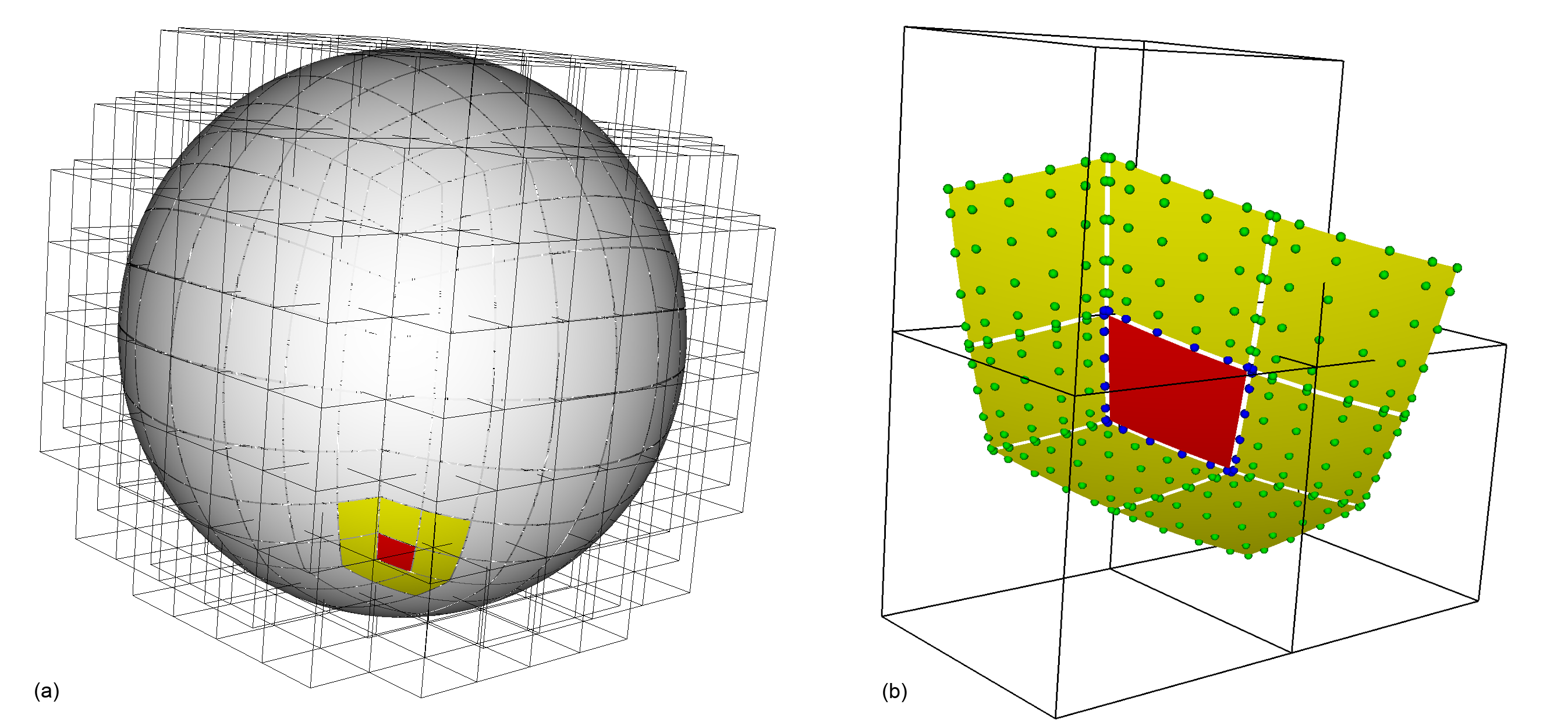
Figure 5: (a) Four level $(D=4)$ IFGF domain decomposition for a sphere (only the finest level boxes are shown). A source surface patch and its neighboring patches are highlighted in red and yellow, respectively. (b) Near-singular and regular points neighboring the red patch are depicted in blue and green, respectively. All interactions from the red patch to itself are singular and, together with the near-singular and neighboring regular interactions are computed by means of the rectangular-polar algorithm described in Section 4. The remaining interactions are accelerated by means of the IFGF algorithm.

To achieve fast computation times, the IFGF method relies on the factorization (39), and it proceeds, as indicated above, by interpolation of the factor $F^{\mathbf{k},d}_{j}(s,\theta,\phi)$. In view of the analyticity and the slowly-oscillating character of the analytic factors $W^{\mathbf{k},d}_{j}$ in (40), accurate interpolation of the factors $F^{\mathbf{k},d}_{j}(s,\theta,\phi)$ can be achieved by polynomial interpolation in relatively coarse $(s,\theta,\phi)$ meshes. In keeping with [3], Chebyshev polynomials of degrees $P_{s}=3$ and $P_{\rm{ang}}=5$ points are used in this paper for interpolation along the radial and angular directions, respectively, but, as indicated in that reference, interpolation methods of higher order may of course be employed as well.

For a given point $x$, the IFGF algorithm produces the desired field $I_{K}(x)$ in (14) by subsequently incorporating, at each level $D,D-1,D-2,\dotsc,3$, all relevant contributions from boxes for which $x$ is a cousin point. (As indicated above, the contributions from nearest neighbor boxes in level $D$ are computed without recourse to the IFGF approach, using directly the methods in Section 4.) Contributions from boxes for which $x$ is not a cousin point at a given level are incorporated at subsequent levels by grouping of boxes into larger boxes. The data necessary for interpolation from a given box is obtained by adding all contributions from the relevant children of that box—each one of which is obtained, once again, by interpolation.

The details of the IFGF algorithm are presented in Algorithm 1. Note that the algorithm does not compute the “local interactions”, that is, the interactions between neighboring boxes on the finest level $(d=D)$. For the scattering solver proposed in this paper, such interactions are evaluated by means of two separate methods, as illustrated in Figure 5 and described in what follows. If the distance from a box’s source points to a neighboring box’s target point $x_{\ell}$ is larger than the proximity distance $\delta$ defined in Section 4, the local interactions are evaluated by means of the algorithm described in Section 4.1. In case the source points and the target point in neighboring boxes are a distance greater than $\delta$, in turn, the quadrature presented in Section 4.2 is used instead. We emphasize that local interactions are computed only in the finest level $(d=D)$. Figure 5(a) shows a four-level $(D=4)$ IFGF domain decomposition for a sphere, where a source patch and its neighbors patches are highlighted in red and yellow, respectively. A close-up view of these patches is shown in Figure 5(b); source-to-neighbor near-singular evaluation points are drawn in blue, while regular evaluation points are depicted in green. All evaluations from a source patch to itself are considered to be singular and are also computed using the algorithms presented in Section 4.2.

1:\\Direct evaluations of the highest-level local interactions.

2:for $B_{\mathbf{k}}^{D}\in\mathcal{R}_{B}$ do

3:    for $C_{\mathbf{k};\boldsymbol{\gamma}}^{D}\in\mathcal{R}_{C}B_{\mathbf{k}}^{D}$ do $\triangleright$ Evaluate $F$ at all relevant interpolation points

4:         for $x=\mathbf{x}(s,\theta,\varphi)\in\mathcal{X}C_{\mathbf{k};\boldsymbol{\gamma}}^{D}$ do

5:             Evaluate and store $F_{\mathbf{k}}^{D}(x)$.

6:         end for

7:    end for

8:end for

9:

10:\\Interpolation onto surface discretization points and parent interpolation points.

11:for $d=D,\ldots,3$ do

12:    for $B_{\mathbf{k}}^{d}\in\mathcal{R}_{B}$ do

13:         for $x\in\mathcal{V}B_{\mathbf{k}}^{d}$ do $\triangleright$ Interpolate at cousin surface points

14:             Evaluate $I_{\mathbf{k}}^{d}(x)$ by interpolation

15:         end for

16:         if $d>3$ then $\triangleright$ Evaluate $F$ on parent interpolation points

17:             Determine parent $B_{\mathbf{j}}^{d-1}=\mathcal{P}B_{\mathbf{k}}^{d}$

18:             for $C_{\mathbf{j};\boldsymbol{\gamma}}^{d-1}\in\mathcal{R}_{C}B_{\mathbf{j}}^{d-1}$ do

19:                 for $x\in\mathcal{X}C_{\mathbf{j};\boldsymbol{\gamma}}^{d-1}$ do

20:                     Evaluate and add $F_{\mathbf{k}}^{d}(x)K(x,y_{\mathbf{k}}^{d})/K(x,y_{\mathbf{j}}^{d-1})$

21:                 end for

22:             end for

23:         end if

24:    end for

25:end for

Algorithm 1 IFGF Algorithm

3.5 IFGF OpenMP parallelization

The proposed OpenMP parallel IFGF method [14] is based in a fundamental manner on an ordering of the IFGF box-cone structure. In particular, the set

$$\mathcal{R}_{C}^{d}:=\bigcup\limits_{\mathbf{k}\in I_{B}^{d}:B_{\mathbf{k}}^{d}\in\mathcal{R}_{B}}\mathcal{R}_{C}B_{\mathbf{k}}^{d},\quad\text{for }3\leq d\leq D.$$ (45)

(cf. Section 3.4) of all level-$d$ cone segments is ordered in accordance to a Morton order (which starts by ordering the set of relevant boxes by means of a three-dimensional Z-looking curve that zig-zags through all boxes [18], and then orders the cone segments associated with each box along angular and radial directions), so that the complete set of interpolating polynomials at any given level $d$ is stored as a single vector, sections of which are subsequently distributed to threads in the OpenMP implementation. The main advantage provided by the IFGF method is that the number of IFGF tasks at each level $d$, which coincides with the number of elements in the set $\mathcal{R}_{C}^{d}$ of level-$d$ cone segments, is a large number that is essentially independent of $d$—so that the set of tasks to be performed at any given level $d$ remains naturally parallelizable for all $d$. In other approaches such as the FMM, the acceleration strategy requires use of decreasing number of increasingly larger structures (as the octree is traversed from the leaves to the root) each one of which is difficult to parallelize—leading to an associated Parallelization Bottleneck [19, 20, 21]. The IFGF approach, in contrast, incorporates large level-independent numbers of OpenMP threads leading to a coarse-grained and well-balanced parallelization resulting in a effective parallel scaling at low memory cost. An extended discussion concerning parallelization of the IFGF method, both under OpenMP and MPI interfaces, can be found in [14].

4 IFGF/RP Evaluation of surface integral operators

The IFGF algorithm introduced in the previous section can be utilized to accelerate the numerical evaluation of integral operators of the form (12) for any given discretization of the scattering boundary $\Gamma$. The RP discretizations utilized in this paper, in turn, are based on use of Chebyshev expansions over each one of the patches $\Gamma^{q}$ introduced in Section 2.3. As indicated in that section, the design of suitable quadrature methods for evaluation of $\mathcal{I}^{q}[\varphi](x)$ requires careful consideration of the relative position of the point $x\in\Gamma$ and the integration patch $\Gamma^{q}$. The “regular” case where $x$ is “far” from $\Gamma^{q}$ is treated easily on the basis of regular Clenshaw-Curtis quadrature (Section 4.1 below) and is subsequently accelerated by means of IFGF; the singular and near-singular cases, for which either $x\in\Gamma^{q}$ or $x$ is “near” $\Gamma^{q}$, in turn, are considered in Section 4.2.

In detail, we consider a general integral operator $\mathcal{I}^{q}$ with singular kernel $K^{q}$ and density $\varphi^{q}$ defined over a component patch $\Gamma^{q}$ is expressed in the parametric form

$$(\mathcal{I}^{q}\varphi)(x)=\int_{[-1,1]^{2}}K^{q}(x,u,v)\varphi^{q}(u,v)J^{q}(u,v)\,dudv,$$ (46)

for $x\in\Gamma$, where $K^{q}(x,u,v)=K(x,y^{q}(u,v))$ and $\varphi^{q}(u,v)=\varphi(y^{q}(u,v))$, and where $J^{q}(u,v)dudv$ denotes the element of area. We refer to $x$ as an “evaluation” or “target” point. In what follows, the “interaction” (46) between an integration patch $\Gamma^{q}$ and a target point $x$ will be said to be singular, near-singular, or regular, depending on whether the distance between the point $x$ and the integration patch $\Gamma^{q}$ is less than or greater than a certain “proximity distance” $\delta>0$. Let

$$\text{dist}\left(x,\Gamma^{q}\right)=\inf\left\{\,|x-y|\,\,|\,\,y\in\Gamma^{q}\right\}$$ (47)

denote the distance from a point $x$ to a patch $\Gamma^{q}$ (where $|\cdot|$ denotes the Euclidean distance). Then, the set of “singular” and “nearly-singular” target points associated with $\Gamma^{q}$ is defined by

$$\Omega_{q}^{s,\delta}=\left\{x\in\Gamma\,\,|\,\,\text{dist}\left(x,\Gamma^{q}\right)\leq\delta\right\}.$$ (48)

In contrast, the set of regular (non-singular) target points is defined by

$$\Omega_{q}^{r,\delta}=\left\{x\in\Gamma\,\,|\,\,\text{dist}\left(x,\Gamma^{q}\right)>\delta\right\}.$$ (49)

Interactions between $\Gamma^{q}$ and $x\in\Gamma$ with $x\in\Omega_{q}^{s,\delta}$ are said to be singular/near-singular; other interactions, wherein $x\in\Omega_{q}^{r,\delta}$, are said to be regular, or, alternatively, non-singular.

The accurate evaluation of the singular and near singular integrals require special treatment, as discussed in Section 4.2, on account of the correspondingly singular or near-singular character of the operator kernels in such cases. The regular integrations, in turn, do not require use of sophisticated quadrature methods, but they involve integration over most of the surface $\Gamma$—and thus give rise to a very large computational costs, for high-frequency problems, if straightforward quadrature methods are used. To avoid the latter problem, the IFGF method introduced in the previous section is utilized in this paper: as shown in Section 2.3, all regular integrations may be expressed in the form (3) for whose evaluation the IFGF method was designed.

The quadrature methods used in this paper are based on representation of $\varphi^{q}$ via Chebyshev expansion for each $q=1,\dotsc,Q$. To incorporate the discrete Chebyshev framework in our context we discretize each patch $\Gamma^{q}$ by means of a surface grid $\Gamma^{q}_{N^{q}_{u},N^{q}_{v}}$ containing $N_{u}^{q}\times N_{v}^{q}$ discretization points obtained as the image of the tensor-product discretization

$$\left\{u_{i}=s^{q}_{i}\,\,|\,\,i=0,\dotsc,N_{u}^{q}-1\right\}\times\left\{v_{j}=t^{q}_{j}\,\,|\,\,j=0,\dotsc,N_{v}^{q}-1\right\},$$

under the surface parametrization $y^{q}$ in equation (10), where $s^{q}_{i}$ and $t^{q}_{j}$ denote the the nodes Chebyshev-Gauss nodes

$$s^{q}_{i}=\cos\left(\pi\frac{2i+1}{2N^{q}_{u}}\right),\qquad t^{q}_{j}=\cos\left(\pi\frac{2j+1}{2N^{q}_{v}}\right),$$ (50)

for $i=0,\dotsc,N^{q}_{u}-1$, $j=0,\dotsc,N^{q}_{v}-1$, and $q=1,\dotsc,Q$. The set of all surface discretization points is denoted by

$$\Gamma_{N}=\bigcup_{q=1}^{Q}\Gamma^{q}_{N^{q}_{u},N^{q}_{v}},$$ (51)

where $N$ denotes the total number of grid points over all component patches.

For $1\leq q\leq Q$, the surface density $\varphi^{q}$ admits the Chebyshev approximation

$$\varphi^{q}(u,v)\approx\sum_{m=0}^{N_{v}^{q}-1}\sum_{n=0}^{N_{u}^{q}-1}a_{n,m}^{q}T_{n}(u)T_{m}(v),$$ (52)

where, in view of the discrete orthogonality property satisfied by Chebyshev polynomials, we have

$$a_{n,m}^{q}=\frac{\alpha_{n}\alpha_{m}}{N_{u}^{q}N_{v}^{q}}\sum_{j=0}^{N_{v}^{q}-1}\sum_{i=0}^{N_{u}^{q}-1}\varphi^{q}(s^{q}_{i},v_{j})T_{n}(s^{q}_{i})T_{m}(v_{j}),\qquad\alpha_{n}=\begin{cases}1,&n=0\\ 2,&n\neq 0.\end{cases}$$ (53)

4.1 Non-singular integration via IFGF acceleration

To evaluate the integral operator (46) at regular target points $x_{\ell}\in\Omega_{q}^{r,\delta}$, we use Fejér’s first quadrature rule, which is based on the nodes (50) and the integration weights

$$w_{j}=w^{J}_{j} =\frac{2}{J}\left[1-2\sum_{\ell=1}^{\left\lfloor J/2\right\rfloor}\frac{1}{4\ell^{2}-1}\cos\left(\ell\pi\frac{2j+1}{J}\right)\right],$$ (54)

so that the value at $x_{\ell}$ is approximated by

$$(\mathcal{I}^{q}\varphi)(x_{\ell})\approx\sum_{j=0}^{N_{v}^{q}-1}\sum_{i=0}^{N_{u}^{q}-1}K^{q}(x_{\ell},s^{q}_{i},t^{q}_{j})\varphi^{q}(s^{q}_{i},t^{q}_{j})J^{q}(s^{q}_{i},t^{q}_{j})\,w^{N_{u}^{q}}_{i}w^{N_{v}^{q}}_{j}.$$ (55)

Evaluating all regular (non-singular) interactions on the basis of (55) results in an algorithm with computing cost of the order of $\mathcal{O}(N^{2})$ operations, whereas the cost of adding all of the singular interactions (by means of the RP algorithm presented in Section 4.2) requires only $\mathcal{O}(N)$ cost—since refinements of discretizations are obtained by partitioning patches and keeping constant the number of points per patch. For acoustically-large problems such a computational cost becomes prohibitively high. Noting that the sum of the regular interactions (55) over all $q$ and for each $\ell$ can manifestly be expressed in the form (14), to address this difficulty we accelerate the evaluation of regular interactions by resorting to the IFGF acceleration method introduced in Section 3. This results in an overall iterative solver with asymptotic $\mathcal{O}(N\log N)$ computing cost. To complete our description of the proposed IFGF-accelerated scattering solver algorithm it therefore suffices to introduce an accurate and efficient algorithm for singular and near-singular interactions—which, as indicated above, is presented in Section 4.2.

4.2 Singular and near-singular integration via the Rectangular-Polar method

To evaluate (46) at a singular or near-singular target point $x\in\Omega_{p}^{s,\delta}$ ($\delta\geq 0$) the RP method proceeds as follows. Replacing the density $\varphi^{q}$ by its Chebyshev expansion (52), in the RP method the integral (46) is numerically approximated by

$$(\mathcal{I}^{q}\varphi)(x) \approx\int_{R}K^{q}(x,u,v)\left(\sum_{m=0}^{N_{v}^{q}-1}\sum_{n=0}^{N_{u}^{q}-1}a_{n,m}^{q}T_{n}(u)T_{m}(v)\right)J^{q}(u,v)\,dudv$$ (56a)

$$=\sum_{m=0}^{N_{v}^{q}-1}\sum_{n=0}^{N_{u}^{q}-1}a_{n,m}^{q}\left(\int_{R}K^{q}(x,u,v)T_{n}(u)T_{m}(v)J^{q}(u,v)\,dudv\right).$$ (56b)

Note that the double integral in this equation does not depend on the density $\phi^{q}$: it depends only on the kernel, a product of Chebyshev polynomials, and the geometry. The proposed method proceeds by accurately precomputing and storing such quantities for all relevant discretization points $x=x_{\ell}$; the algorithm is completed by direct evaluation of the sum (56b). In other words, letting

$$\beta_{n,m}^{q,\ell}=\int_{R}K^{q}(x_{\ell},u,v)T_{n}(u)T_{m}(v)J^{q}(u,v)\,dudv,$$ (57)

the algorithm obtains the value of $\mathcal{I}^{q}$ at all target points $x_{\ell}\in\Omega_{p}^{s,\delta}$ on the basis of the expression

$$(\mathcal{I}^{q}\varphi)(x_{\ell})=\sum_{m=0}^{N_{v}^{q}-1}\sum_{n=0}^{N_{u}^{q}-1}a_{n,m}^{q}\,\beta_{n,m}^{q,\ell}.$$ (58)

To obtain (57) at an evaluation point $x_{\ell}\in\Gamma$ the algorithm utilizes the point $x^{q}_{\ell}\in\Gamma^{q}$ that is closest to $x_{\ell}$, or, more precisely, the parameter-domain coordinates of $x^{q}_{\ell}$ in the patch $\Gamma^{q}$. If $x^{q}_{\ell}$ is itself a grid point of $\Gamma^{q}$, $x^{q}_{\ell}=x_{\ell}=y^{q}(\bar{u}_{\ell}^{q},\bar{v}_{\ell}^{q})$, then its parameter-space coordinates in the patch $\Gamma^{q}$ are of course equal to $(\bar{u}_{\ell}^{q},\bar{v}_{\ell}^{q})$. More generally, $(\bar{u}_{\ell}^{q},\bar{v}_{\ell}^{q})$ is obtained as the distance minimizer:

$$(\bar{u}_{\ell}^{q},\bar{v}_{\ell}^{q})=\operatorname*{arg\,min}_{(u,v)\in[-1,1]^{2}}\left\|x_{\ell}-y^{q}(u,v)\right\|.$$ (59)

Following [2], for robustness and simplicity our algorithm tackles the minimization problem (59) by means of the golden section search algorithm.

Next, we apply a one-dimensional change of variables to each coordinate in the $uv$-parameter space to construct a clustered grid around each given target node. To this end we consider the following one-to-one, strictly monotonically increasing, and infinitely differentiable function $w:[0,2\pi]\to[0,2\pi]$, with parameter $d\geq 2$ (proposed in [22, Section 3.5]):

$$w(\tau;d)=2\pi\frac{[\nu(\tau)]^{d}}{[\nu(\tau)]^{d}+[\nu(2\pi-\tau)]^{d}},\qquad 0\leq\tau\leq 2\pi,$$ (60)

where

$$\nu(\tau;d)=\left(\frac{1}{d}-\frac{1}{2}\right)\left(\frac{\pi-\tau}{\pi}\right)^{3}+\frac{1}{d}\left(\frac{\tau-\pi}{\pi}\right)+\frac{1}{2}.$$ (61)

It can be shown that $w$ has vanishing derivatives up to order $d-1$ at the interval endpoints. Then, the following change of variables

$$\xi_{\alpha}(\tau;d)=\begin{cases}\alpha+\left(\frac{\text{sgn}(\tau)-\alpha}{\pi}\right)w(\pi|\tau|;d),&\text{ for }\alpha\neq\pm 1,\\ \alpha-\left(\frac{1+\alpha}{\pi}\right)w(\pi\left|\frac{\tau-1}{2}\right|;d),&\text{ for }\alpha=1,\\ \alpha+\left(\frac{1-\alpha}{\pi}\right)w(\pi\left|\frac{\tau+1}{2}\right|;d),&\text{ for }\alpha=-1,\end{cases}$$ (62)

has the effect of clustering points around $\alpha$. Fejér’s rule (Section 4.1) applied to the integral (57), transformed using the change of variables (62), yields the approximation

$$\beta_{n,m}^{q,\ell}\approx\sum_{j=0}^{N_{\beta}-1}\sum_{i=0}^{N_{\beta}-1}K^{q}(x_{\ell},u_{i}^{q,\ell},v_{j}^{q,\ell})T_{n}(u_{i}^{q,\ell})T_{m}(v_{j}^{q,\ell})J^{q}(u_{i}^{q,\ell},v_{j}^{q,\ell})\,w_{i}^{u,q,\ell}w_{j}^{v,q,\ell},$$ (63)

where

$$u_{i}^{q,\ell} =\xi_{\bar{u}_{\ell}^{q}}(s_{i};d),\quad w_{i}^{u,q,\ell}=\frac{d\xi_{\bar{u}_{\ell}^{q}}}{d\tau}(s_{i};d)\,w_{i},$$ (64)

$$v_{j}^{q,\ell} =\xi_{\bar{v}_{\ell}^{q}}(s_{j};d),\quad w_{j}^{v,q,\ell}=\frac{d\xi_{\bar{v}_{\ell}^{q}}}{d\tau}(s_{j};d)\,w_{j},$$ (65)

for $i,\,j=0,\dotsc,N_{\beta}-1$. To avoid division by zero, we set the kernel $K^{q}$ to zero at integration points where the distance to the target point is less than some prescribed tolerance, usually on the order of $10^{-14}$. This completes the singular and near-singular integration algorithm, and, thus, incorporating the iterative linear algebra solver GMRES, the proposed overall IFGF-accelerated high-order integral solver for the problem (2).

5 Numerical results

This section presents numerical results that demonstrate the character of the proposed IFGF-accelerated acoustic scattering solvers described in previous sections. For comparison, results obtained using the $\mathcal{O}(N^{2})$ non-accelerated Chebyshev-based scattering solvers introduced in [2] are also included. Both the accelerated and non-accelerated solver are implemented using OpenMP for shared-memory parallelism.

After solving (7) for the density $\varphi$, the far field pattern $u^{\infty}$ can be obtained from

$$u^{\infty}(\hat{x})=\frac{1}{4\pi}\int_{\Gamma}\left\{\frac{\partial}{\partial\nu(y)}e^{-\text{i}k\hat{x}\cdot y}-\text{i}\gamma e^{-\text{i}k\hat{x}\cdot y}\right\}\varphi(y)\,dS(y),\quad\hat{x}\in\mathbb{S}^{2},$$ (66)

where $\mathbb{S}^{2}$ denotes the unit sphere and $\Gamma$ is the scatterer’s boundary. The far field is computed over a uniformly-spaced unit spherical grid

$$\mathbb{S}^{2}_{N}=\left\{(\phi_{m},\theta_{n})\in[0,\pi]\times[0,2\pi]\,\,|\,\,1\leq m\leq N_{\phi},\,1\leq n\leq N_{\theta}\right\},$$ (67)

with $\phi_{m}=(m-1)\Delta\phi,\,\theta_{n}=(n-1)\Delta\theta$ and where the spacings are defined as $\Delta\phi=\pi/(N_{\phi}-1)$ and $\Delta\theta=2\pi/(N_{\theta}-1)$, respectively; specific values of $N_{\phi}$ and $N_{\theta}$ are given in each example’s subsection. Given the discrete values of exact (reference) far field modulus $|u^{\infty}_{m,n}|$ and approximate far field modulus $|\tilde{u}^{\infty}_{m,n}|$ ($1\leq m\leq N_{\phi},\,1\leq n\leq N_{\theta}$), the maximum far field relative error $\varepsilon_{\textit{far}}$ over $\mathbb{S}^{2}_{N}$ given by

$$\varepsilon_{\textit{far}}=\max_{(m,n)\in\mathbb{S}^{2}_{N}}\left\{\frac{|\ |u_{m,n}^{\infty}|-|\tilde{u}_{m,n}^{\infty}|\ |}{|u_{m,n}^{\infty}|}\right\},$$ (68)

is reported in each case.

Similarly, substituting the solution $\varphi$ in the combined-layer representation (3) we evaluate and display the scattered field $u^{s}$ over near field planes that are parallel to the $xy$-, $xz$-, or $yz$-planes. For example, we evaluate fields (incident, scattered, and total) at every point of a uniformly-spaced two-dimensional $xy$-planar grid $\mathbb{P}_{N}^{xy}(z_{0})$ at $z=z_{0}$ defined by

$$\mathbb{P}_{N}^{xy}(z_{0})=\left\{(x_{m},y_{m},z_{0})\in[x_{min},x_{max}]\times[y_{min},y_{max}]\times\{z_{0}\}\,\,|\,\,1\leq m\leq N_{x},\,1\leq n\leq N_{y}\right\},$$ (69)

where the grid points are given by $x_{m}=(m-1)\Delta x,\,y_{n}=(n-1)\Delta y$ and the grid spacings are $\Delta x=(x_{max}-x_{min})/(N_{x}-1)$ and $\Delta y=(y_{max}-y_{min})/(N_{y}-1)$. Near field planar grids parallel to the $xz$- and $yz$-plane are defined analogously. Denoting the exact (or reference) and approximate modulus of the total field at each point of $\mathbb{P}_{N}^{xy}(z_{0})$ by $v_{m,n}$ ($=|u_{m,n}^{s}+u^{i}_{m,n}|$) and $\tilde{v}_{m,n}$ ($=|\tilde{u}_{m,n}^{s}+u^{i}_{m,n}|$), respectively, we define the near field (total magnitude) relative error $\varepsilon_{\textit{near}}$ over $\mathbb{P}_{N}^{xy}(z_{0})$ by

$$\varepsilon_{\textit{near}}=\max_{(m,n)\in\mathbb{P}_{N}^{xy}(z_{0})}\left\{\frac{|v_{m,n}-\tilde{v}_{m,n}|}{|v_{m,n}|}\right\}.$$ (70)

The numerical results presented in what follows were obtained using 28 cores in a single Intel Xeon Platinum 8276 2.20 GHz computer. The images presented were generated using the visualization software VisIt [23]. Solutions to the complex-coefficient linear systems that arise from discretizations of the boundary integral equation (7) were obtained by means of a complex-arithmetic GMRES iterative solver [1]. Following [6], we utilize the value

$$\gamma=\max\{3,A/\lambda\}$$ (71)

of the coupling parameter in the combined-layer equation (7), where $A$ denotes the diameter of the scatterer. Detailed computational studies indicate that, to reach a given residual tolerance, this value reduces the number of GMRES iterations by a factor of $5-10$ vs. the iteration numbers required when the oft considered value $\gamma=k$ is used. Per Remark 1, in all cases the values $n_{C,0}=2$ and $n_{S,0}=1$ were utilized.

5.1 Scattering by a sphere

This section concerns the classical problem of scattering of plane waves by sound-soft spheres, for which the well-known closed-form Mie series far field expression is used to compute relative errors [24]. Spheres of various acoustical sizes are considered, ranging from $4\lambda$ to $128\lambda$ in diameter. In all cases the number of IFGF levels was selected so that the finest-level IFGF box side length is approximately $0.5\lambda$.

Table 1 demonstrates the character of both, the IFGF-accelerated solver and the non-accelerated solver, via applications to problems of scattering by spheres of diameters ranging from $4$ to $128$ wavelengths. In all cases the GMRES residual tolerance was set to $10^{-4}$. We report the total number of unknowns, the size of the sphere in wavelengths, the time required to compute one GMRES iteration, the total number of iterations required to achieve the prescribed residual, and the field relative error. Far field relative errors are presented over the spherical grid (67) with $(N_{\phi},N_{\theta})=(200,200)$. The computing times per iteration displayed in this table for the non-accelerated algorithm, grow by a factor of around $14.8-15.7$ as the number of points per dimension in each surface patch is doubled (so that the overall number $N$ of unknowns is quadrupled), which is consistent with the expected quadratic complexity of the algorithm. The corresponding costs for the IFGF-accelerated solver, on the other hand, scale like $\mathcal{O}(N\log N)$, as illustrated in Figure 6. In all cases, solutions with errors of the order of $10^{-4}$ were obtained.

		Nonaccelerated			Accelerated
Unknowns	Size	Time (1 iter.)	Iters.	$\varepsilon_{\textit{far}}$	Levels	Time (1 iter.)	Iters.	$\varepsilon_{\textit{far}}$
13,824	4$\lambda$	0.5 s	12	$1.1\cdot 10^{-4}$	4	0.2 s	12	$1.3\cdot 10^{-4}$
55,296	8$\lambda$	7.4 s	14	$8.9\cdot 10^{-5}$	5	1.0 s	14	$1.1\cdot 10^{-4}$
221,184	16$\lambda$	116.4 s	14	$2.6\cdot 10^{-5}$	6	4.6 s	14	$6.3\cdot 10^{-5}$
884,736	32$\lambda$	1862.4 s (est.)	$\--$	$\--$	7	19.4 s	16	$2.9\cdot 10^{-5}$
3,538,994	64$\lambda$	8.3 h (est.)	$\--$	$\--$	8	83.1 s	18	$6.0\cdot 10^{-5}$
14,155,776	128$\lambda$	132.8 h (est.)	$\--$	$\--$	9	443.2 s	21	$3.8\cdot 10^{-4}$

Table 1: Performance of both, the IFGF-accelerated solver and the non-accelerated solver, for problems of scattering by spheres of diameters ranging from $4$ to $128$ wavelengths. The table summarizes the total number of surface unknowns, sphere size in wavelengths, number of IFGF levels used, time required to compute one GMRES iteration, total number of iterations, and far field relative error $\varepsilon_{\textit{far}}$. In all cases the GMRES residual tolerance was set to $10^{-4}$.

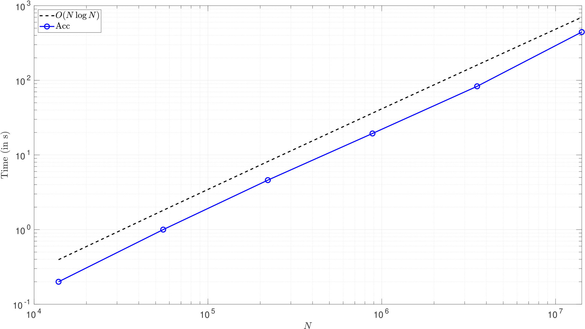
Figure 6: Computing times, in seconds, required by the IFGF-accelerated solver, as a function of the total number $N$ of discretization points (line-circle markers), for the problem of acoustic scattering by spheres. For reference, the figure includes a curve parallel the graph of $CN\log N$ with slope $C=0.3\cdot 10^{-5}$ (dashed line).

The reduced complexity of the IFGF-based algorithm has a significant impact on computing times. At $128$ wavelengths, the computing time per iteration required by the non-accelerated solver are over $1000$ times larger than those required by the accelerated method; for larger problems, the difference in compute times grows as expected from the complexity estimates for the two methods. It is worthwhile to note that, in all cases for which iteration numbers are presented for both methods, the non-accelerated and accelerated solvers require the same number of GMRES iterations to meet the prescribed residual tolerance. Additionally, the errors for both algorithms are comparable: the non-accelerated solver yields solutions for the $4,\,8$ and $16$ wavelength problems with an average relative error of $1.1\cdot 10^{-4}$, while errors obtained with the accelerated method average $1.3\cdot 10^{-4}$ across the entire $4$ to $128$ wavelength range.

5.2 Comparisons with FMM-based solvers

This section provides comparisons of the proposed IFGF/RP algorithm with two recent FMM accelerated scattering solvers for the problem considered in this paper. The first test case considered, whose results are presented in Table 2, examines the convergence of the far field scattered by a spherical scatterer as a function of the number of iterations in the GMRES iterative solver, for the formulation (7) and with the value of $\gamma$ given in (71). The selected problem, a sphere $2$m in diameter under illumination at the frequency $f=14.880$ KHz, coincides with the third test case considered in [17, Table 2] for the single-layer, FMM-accelerated formulation introduced in that reference. The present results compare favorably with the one provided in that reference: using 1,572,864 degrees of freedom (DoF), a total of 8 iterations of the present solver suffice to yield a far-field accuracy of $1.3\cdot 10^{-3}$ whereas 1,123 iterations and $8,984,640$ DoFs are utilized in that reference to obtain a far-field error of $3\cdot 10^{-3}$. Clearly, the second-kind formulation (7) utilized in this paper is greatly advantageous, in spite of the fact of its requirement of evaluation of two operators (the single- and double-layer potentials) instead of one operator in the single-layer formulation used in [17]. The computing times per iteration required by IFGF/RP algorithm to achieve this accuracy also compare favorably: each two-operator (single and double layer) iteration of the present solver requires a computing time of $58.3$s in a total of 28 cores, whereas the one-operator (single layer) FMM-based iteration in [17] requires $46.8$s in a total of 512 cores.

# Iters.	2	4	8	12
$\varepsilon_{\textit{far}}$	$1.9\cdot 10^{-1}$	$1.8\cdot 10^{-2}$	1.3 $\cdot 10^{-3}$	$5.8\cdot 10^{-4}$
Run time (in s, at 58.3 s/iter)	116.6	233.2	466.4	699.6

Table 2: Far-field relative error resulting from the proposed accelerated solver as a function of the number of GMRES iterations incurred, for a configuration considered in [17, Table 2]: scattering by a sphere $2$ m in diameter at a frequency of $f=14.88$ KHz. At the speed of sound assumed in that paper ($c=343$ m/s), the sphere is approximately $86.8\lambda$ in diameter ($2\mathrm{m}/\lambda=2\mathrm{m}f/c=86.8$). The results presented in the present table were obtained on the basis of a total of $1,572,864$ unknowns.

A second point of reference is provided in the publication [16], which demonstrates an FMM-accelerated QBX algorithm for a problem of scattering by an aircraft geometry with a maximum dimension of approximately $64\lambda$, on a 20-core 2.30 GHz Intel Xeon E5-2650 v3 machine. A sequence of geometry-specific optimizations listed in [16, Fig. 11] reduces a certain reference FMM computing times by certain percentages. The optimized, 14 million DoF implementation is reported to run at computing times for the double-layer and single-layer operators of 1600 seconds and 900 seconds, respectively, for a total of 2,500 seconds in the combined formulation used, to achieve an estimated accuracy of $2.5\cdot 10^{-3}$. Results of a run containing a similar number of degrees of freedom on a sphere, but for the much larger acoustical size of $128\lambda$ in diameter, are presented in the last row of Table 2—showing a 28-core computing time (2.20 GHz cores) of 443.2s per iteration, together with an error of $3.8\cdot 10^{-4}$. In all, these experiments and comparisons suggest that the proposed IFGF/RP method provides a valuable new tool for the solution of high frequency scattering problems.

5.3 Scattering by a submarine geometry

Owing to its importance in detection and tracking applications, the accurate simulation of problems of acoustic scattering involving submarine vehicles is the subject of ongoing research  [25, 26, 27, 28, 29, 30, 31]. This section demonstrates the character of the proposed IFGF accelerated solver in such a context: it concerns problems of acoustic scattering by realistic submarine configurations of up to $80$ wavelengths in acoustical size. The submarine model used, comprising the main hull, sail, diving planes, rudders, and a five-blade propeller, is depicted in Figure 7. The complete submarine geometry is contained in the bounding region $[-3.2,3.2]\times[-1.9,2.8]\times[-19.2,10.9]$. Figures 7(b) and 7(c) display portions of a surface representation containing $4,560$ patches, each of which is discretized by $6\times 6$ points.

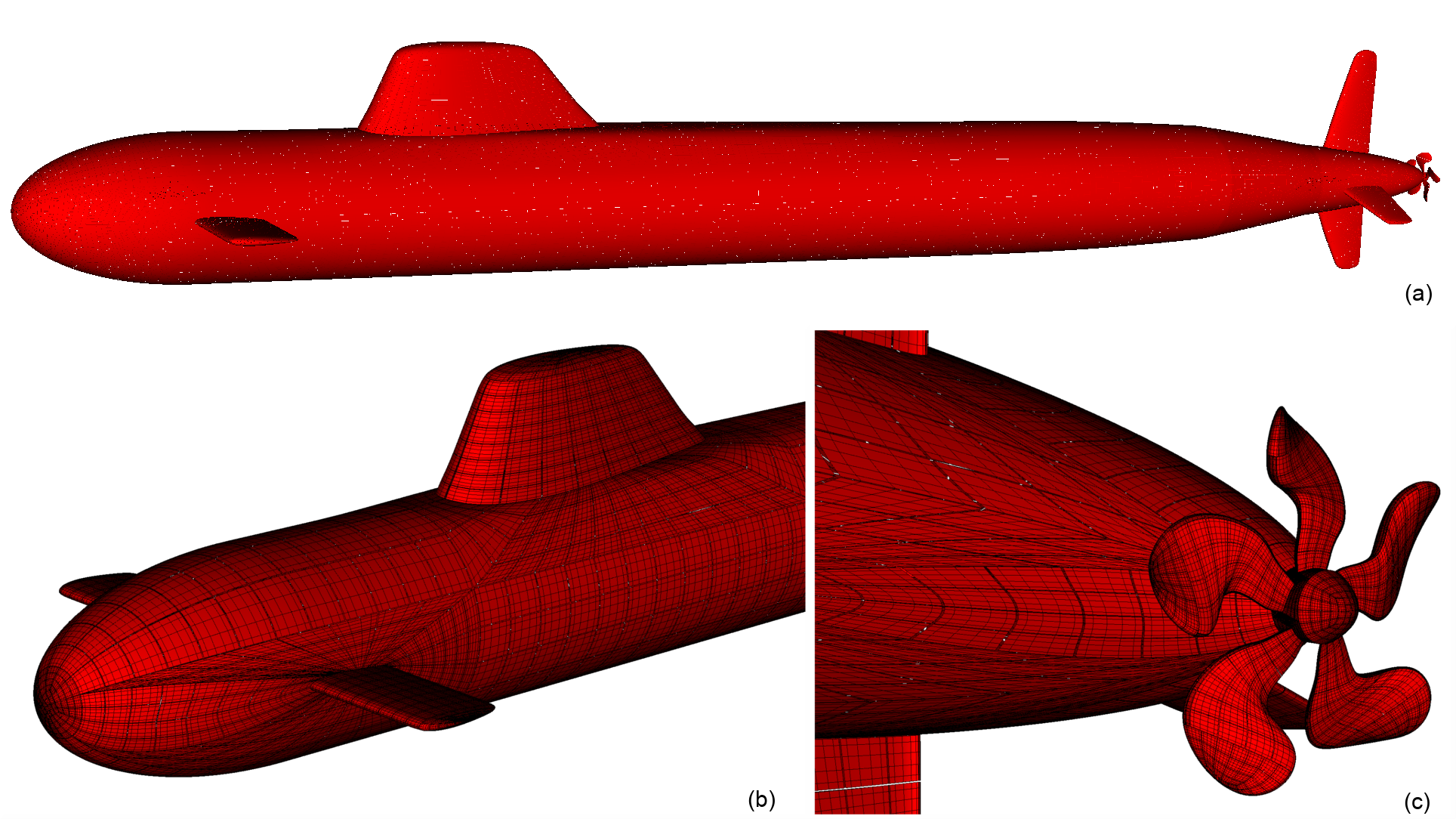
Figure 7: Submarine model and surface mesh containing a total of 164,160 points. The submarine hull is aligned with the $z$-axis and the sail is parallel to the $+y$-axis; the front of the vessel points in the $+z$-direction.

We consider plane wave scattering for two cases: a) head-on incidence and b) oblique incidence. The incident field is a plane wave $u^{i}$ that travels along the wave direction $\hat{k}$ and is given by

$$u^{i}(x)=e^{\text{i}k\hat{k}\cdot x},\qquad\hat{k}=\begin{pmatrix}\cos\theta\sin\phi\\ \sin\theta\sin\phi\\ \cos\phi\end{pmatrix},$$ (72)

where $x=(x_{1},x_{2},x_{3})$ denotes the position vector, $k>0$ is a given wavenumber, and $(\theta,\phi)\in[0,2\pi)\times[0,\pi]$. Since the bow of the submarine points in the $+z$-direction, “head-on” incidence corresponds to $(\theta,\phi)=(0,\pi)$ in (72). For the oblique incidence case we set $(\theta,\phi)=(0,5\pi/4)$.

To verify the accuracy of the IFGF-accelerated solver in the present case, we conducted convergence studies for the submarine structures of acoustical sizes (measured from the bow to the propeller cap) of $10\lambda,\,20\lambda$, $40\lambda$ and $80\lambda$. In all cases the number of IFGF levels was chosen so that the side length of the smallest, (finest level) boxes is approximately $0.8\lambda$, and the GMRES residual tolerance was set to $10^{-3}$. We start our sequence of test cases with a $10\lambda$ vessel whose geometry is represented by $1,140$ surface patches, each of which has $6\times 6$ points. As the size of the problem is doubled, the geometry is partitioned from the previous size so that every patch is split into four subpatches while keeping the number of points per patch fixed. Thus, for example, the $20\lambda$ problem uses four times as many surface points as the $10\lambda$ one. This is admittedly a suboptimal strategy in this case (since, after a certain level $d$, the smaller patches on the propeller, rudders and diving planes are the only ones that would provide acceleration via further partitioning), which, however, simplifies the code implementation (cf. the discussion concerning adaptivity at the end of Section 3.3). As indicated in [3], the IFGF method can be extended to incorporate a box octree algorithm that adaptively partitions a geometry so that boxes containing a (small) prescribed number of points are not further partitioned, which eliminates the difficulty posed in the problem at hand by finely discretized structures such as the propeller, rudders and diving planes. While such an addition is left for future work, as demonstrated in Table 3, even the simple uniform-partition IFGF algorithm we use here is sufficient to simulate scattering by a realistic submarine geometry for up to $80$ wavelengths in size with several digits of accuracy and using only modest computational resources. For example, the $656,640$ unknowns, $40\lambda$ run for head-on incidence, required a computing time of $313$ seconds per iteration and a total of $78$ iterations. The fully adaptive version of the IFGF algorithm, which, as mentioned above, is not pursued in this paper, should yield submarine-geometry computing times consistent with those shown in Tables 1 and 4 for the sphere and nacelle geometries, respectively.

			Front Incidence	Oblique Incidence
Unknowns	Size	IFGF levels	$\varepsilon_{\textit{near}}$	$\varepsilon_{\textit{near}}$
41,040	10$\lambda$	5	$2.4\cdot 10^{-4}$	$6.8\cdot 10^{-4}$
164,160	20$\lambda$	6	$1.8\cdot 10^{-4}$	$6.0\cdot 10^{-4}$
656,640	40$\lambda$	7	$2.1\cdot 10^{-4}$	$1.7\cdot 10^{-4}$
2,626,560	80$\lambda$	8	$2.1\cdot 10^{-4}$ (est.)	$4.8\cdot 10^{-4}$ (est.)

Table 3: Near field errors resulting from applications of the IFGF accelerated acoustic solver to the submarine geometry depicted in Figure 7, with acoustical sizes ranging from $10$ to $80$ wavelengths. Errors were evaluated by means of convergence studies, as detailed in the text, except for the $80$-wavelength case, for which, as mentioned in the text, an estimate was used. In all cases the residual tolerance for the integral density was set to $10^{-3}$.

Near field relative errors (70) for front (head-on) and oblique plane wave incidence are presented in Table 3. For each problem, the near field errors $\varepsilon_{\textit{near}}$ were obtained over the planar region $\mathbb{P}_{N}^{xy}(z_{0})$ (equation (69)) with $[x_{min},x_{max}]\times[y_{min},y_{max}]=[-12,12]^{2},\,z_{0}=-25$ and $N_{x}=N_{y}=260$. The reference solution was obtained with the same number of surface patches as the target discretization but using $8\times 8$ points per patch and a residual tolerance of $10^{-5}$. (Thus, the reference solution uses nearly twice as many discretization points and it satisfies a more stringent convergence condition.) The numerical results indicate that the solution accuracy is consistent for both front and oblique incidence and for all acoustical sizes considered. The relative errors for the $10\lambda,\,20\lambda$, and $40\lambda$ for the front and oblique incidence problems achieve average accuracies of $2.1\cdot 10^{-4}$ and $4.8\cdot 10^{-4}$, respectively; these values where used to estimate the expected relative errors in the $80$-wavelength case by simple averaging.

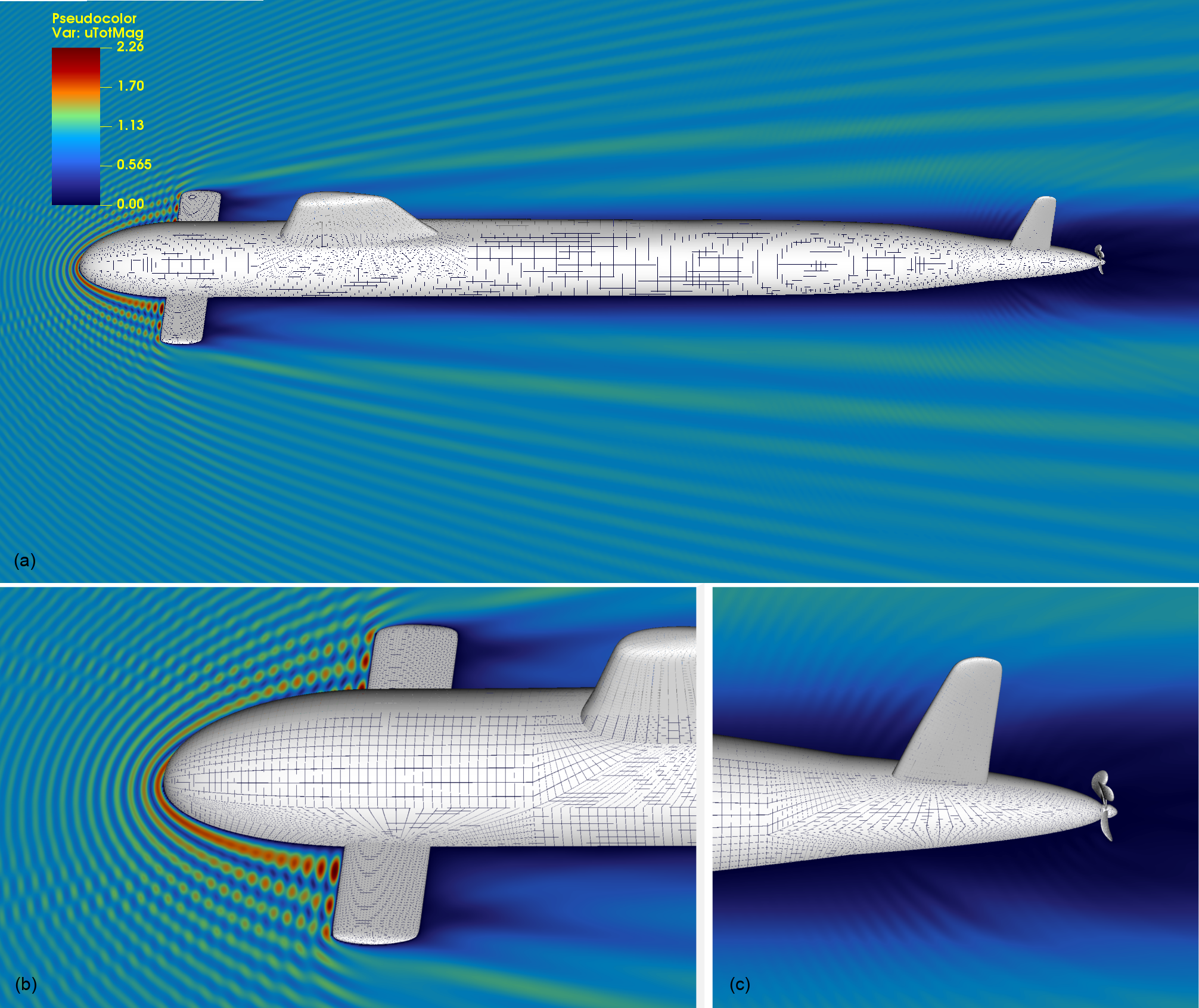
Figure 8: Total field magnitude $|u(x)|=|u^{i}(x)+u^{s}(x)|$ pseudo-color plots for an $80$-wavelength submarine. The field is displayed over a uniform grid of $1040\times 1760$ points $(x,z)\in[-12,12]\times[-25,15]$. The incident plane wave impinges on the vessel head-on, which corresponds to the wave direction $\hat{k}$ in (72) with $(\theta,\phi)=(0,\pi)$.

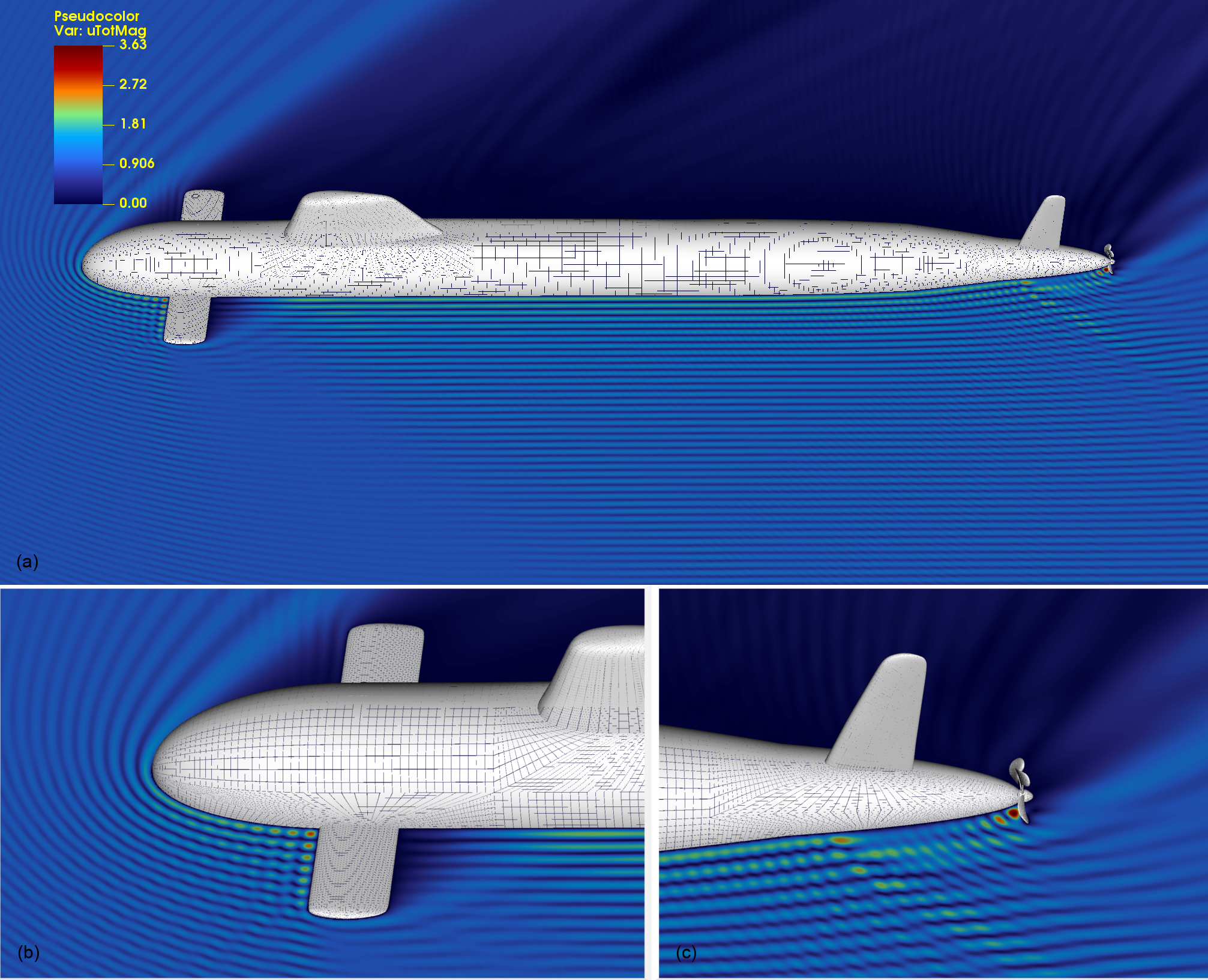
Figure 9: Total field magnitude $|u(x)|=|u^{i}(x)+u^{s}(x)|$ pseudo-color plots for an $80$-wavelength submarine. The field is displayed over a uniform grid of $1040\times 1760$ points $(x,z)\in[-12,12]\times[-25,15]$. The incident plane wave impinges on the vessel at an oblique angle, which corresponds to the wave direction $\hat{k}$ in (72) with $(\theta,\phi)=(0,5\pi/4)$.

Figure 8 presents pseudo-color near field plots of the total field magnitude $|u(x)|=|u^{i}(x)+u^{s}(x)|$ resulting for front plane wave incidence on an $80$-wavelength submarine. The field is plotted over a uniform $1040\times 1760$ point planar grid $\mathbb{P}_{N}^{xz}(y^{0})$ for $(x,z)\in[-12,12]\times[-25,15]$ and $y^{0}=0$. The incident plane wave impinges on the vessel head-on and we see in Figures 8(a) and 8(b) that the strongest interaction occurs around the bow and diving planes (also known as hydroplanes) of the ship. Shadow regions are visible immediately behind the hydroplanes as well as along the hull, particularly in the aft of the ship where the body tapers. Figure 8(c) shows that the wider sections of the ship obstruct the propeller from most incoming waves and, as a consequence, there is minimal interaction in this region. Figure 9, in turn, shows near field pseudo-color plots for the same $80$-wavelength submarine but this time for oblique plane wave incidence. The total field magnitude is plotted over the uniform grid $\mathbb{P}_{N}^{xz}(y^{0})$ described in the previous paragraph. In this case the wave interaction is markedly different. We see the expected shadow region in the opposite side of the incoming wave but there is now clear evidence of wave interaction between the hull and diving planes as well as around the rudders and propeller. In addition to multiple scattering, the close-up views in Figures 8(b), 9(b) and 9(c) show the formation of bright spots near the junction of the left hydroplane and hull and in the vicinity of the propeller. each one of which spawns a scattered wave propagating in forward directions.

5.4 Scattering by an aircraft nacelle

The simulation of aircraft engine noise has been the subject of intense research for the past several decades due to its importance in civil aviation applications [32, 33, 34, 35, 36]. This section presents simulations of sound scattering by the turbofan engine nacelle model shown in Figure 10 in accordance with the boundary value problem (2). Although such acoustic simulations do not account for many of the complexities associated with engine noise, such as, e.g., fluid flow, density gradients, and noise generation, as illustrated by the aforementioned references, acoustic models such as the one considered here play significant roles in the modeling of engine noise. According to the nacelle wall liner case study [37], for example, under typical operating conditions, engine nacelle noise occurs in the $125\--5650$ Hz frequency range. For a typical airliner engine that is around 5 m long, these frequencies correspond to acoustical sizes between $2$ and $82$ wavelengths. The engine nacelle geometry used in the simulations that follow is depicted in Figures 10(a) and 10(b); it comprises an outer housing and a center shaft. The entire two-piece nacelle structure is contained inside the bounding region $[-1.5,1.5]\times[-1.5,1.5]\times[-3.27,3.27]$. The center shaft is aligned with the $z$-axis, with the tip of the shaft pointing towards the positive direction. A discretization containing 8,576 surface patches with $6\times 6$ points per patch is shown in Figure 10(c); for future reference, note that the inset image shows that the mesh is not rotationally symmetric, e.g. near the tip of the shaft.

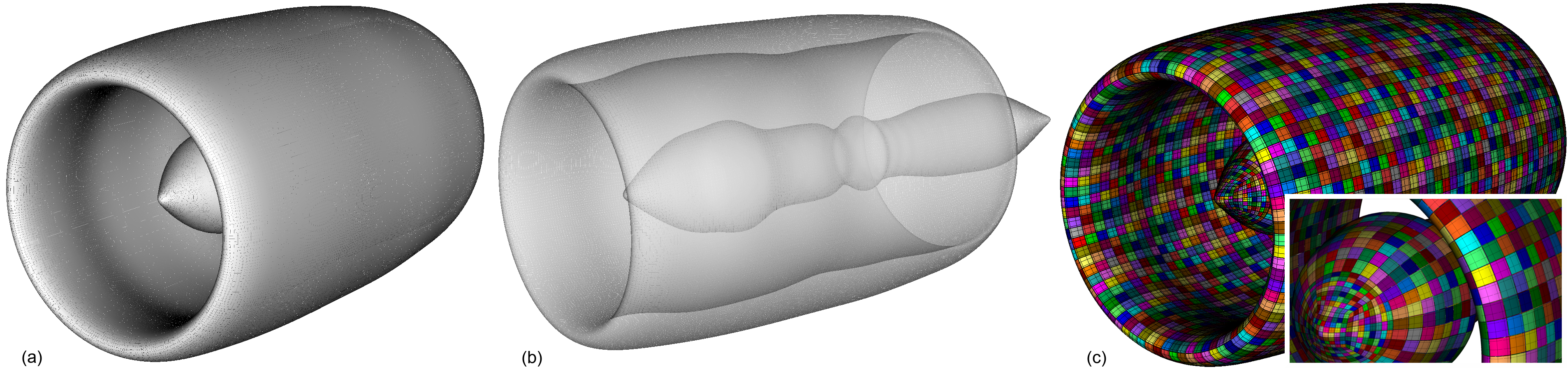
Figure 10: (a) Aircraft engine nacelle model, (b) translucent view of the geometry where the center shaft is visible, and (c) 8,576-surface-patch discretization with $6\times 6$ points per patch (for clarity, only every other mesh point is plotted).

Two types of incident fields were used: a) A plane wave that travels towards the $-z$-axis, so that it impinges on the nacelle head-on; and, b) A set of eight point sources placed inside the housing around the center shaft. As in the submarine example, the plane wave incident field is given by (72) with $(\theta,\phi)=(0,\pi)$. The incident field b), on the other hand, serves as a simple model for fan noise generation inside the nacelle and is given by

$$u^{i}(x)=\sum_{j=1}^{8}\frac{e^{\text{i}k|x-x^{j}|}}{|x-x^{j}|},\quad\text{with point source locations}\quad x^{j}=(x^{j}_{1},x^{j}_{2},x^{j}_{3})=(\cos\alpha_{j},\sin\alpha_{j},2),$$ (73)

where $\alpha_{j}=(j-1)\Delta\alpha+\pi/8$, for $j=1,\dotsc,8$, and $\Delta\alpha=\pi/4$; as illustrated in panel (b) of Figure 12.

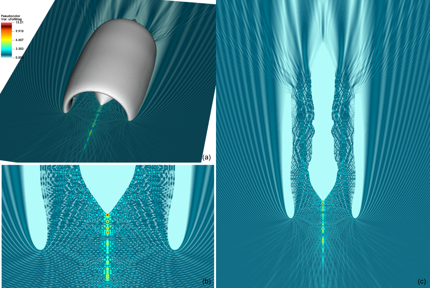
Figure 11: Total field magnitude $|u(x)|=|u^{i}(x)+u^{s}(x)|$ pseudo-color plots for an $82$-wavelength aircraft nacelle. The field is plotted over a uniform grid of $2800\times 4000$ points $(x,z)\in[-4,4]\times[-5,6]$. The nacelle is aligned with the $z$-axis and its front points towards the positive $z$-direction. The incident plane wave impinges on the geometry head-on, traveling towards the negative $z$-axis.

				Plane Wave Incidence		Point Source Incidence
Unknowns	Size	IFGF levels	Time (1 iter.)	Tot. iter.	$\varepsilon_{\textit{near}}$	Tot. iter.	$\varepsilon_{\textit{near}}$
77,184	10.2$\lambda$	6	2.0 s	33	$1.5\cdot 10^{-3}$	39	$4.1\cdot 10^{-3}$
308,736	20.5$\lambda$	7	8.7 s	47	$2.2\cdot 10^{-3}$	59	$4.0\cdot 10^{-3}$
1,234,944	40.9$\lambda$	8	40.4 s	55	$6.7\cdot 10^{-4}$	115	$2.4\cdot 10^{-3}$
4,939,776	81.8$\lambda$	9	176.4 s	65	$1.5\cdot 10^{-3}$ (est.)	219	$3.5\cdot 10^{-3}$ (est.)

Table 4: Near field relative errors $\varepsilon_{\textit{near}}$ resulting from applications of the IFGF accelerated acoustic solver to the nacelle geometry depicted in Figure 10, for plane wave and multiple point-source incidence, and with acoustical sizes ranging from $10.2$ to $81.9$ wavelengths. As detailed in the text, errors were evaluated by means of convergence studies, except for the $81.9$-wavelength case, for which an estimate was used. The table additionally summarizes the total number of surface unknowns, the nacelle size in wavelengths, the maximum number of IFGF levels, the time required per GMRES iteration, and the total number of iterations incurred. In all cases the residual tolerance for the integral density was set to $10^{-3}$.

Table 4 presents near field errors $\varepsilon_{\textit{near}}$ resulting from use of the proposed accelerated solver for an aircraft engine nacelles $10.2,\,20.5$, $40.9$ and $81.8$ wavelengths in size under both plane wave and multiple point-source incidence. The number of IFGF levels is selected so that the finest-level IFGF box side length is approximately $0.6\lambda$ in all cases, and the GMRES residual tolerance was set to $10^{-3}$. The total near field relative error $\varepsilon_{\textit{near}}$ was evaluated over a near field planar grid $\mathbb{P}_{N}^{xy}(z_{0})$, where $[x_{min},x_{max}]\times[y_{min},y_{max}]=[-4,4]^{2},\,z_{0}=-5$, and $N_{x}=N_{y}=400$. The reference solution used for error estimation was obtained with the same number of surface patches but using $8\times 8$ points per patch and a residual tolerance of $10^{-5}$, which gave rise to an increase in the number of iterations required for convergence to the prescribed tolerance by only $8\--14$ iterations. In addition to the near field relative error, Table 4 also includes the total number of unknowns, the nacelle size in wavelengths, the time required per iteration, and the total number of GMRES iterations required to meet the $10^{-3}$ residual tolerance. Note that, as the problem size increases from $10.2\lambda$ to $20.5\lambda$, $20.5\lambda$ to $40.9\lambda$, and $40.9\lambda$ to $81.8\lambda$, and the number of unknowns is quadrupled in each case, the computing cost per iteration increases by a factor of only $4.4,\,4.6$ and $4.4$, respectively (which is consistent with an $\mathcal{O}(N\log N)$ complexity), and not the 16-fold cost increase per wavelength doubling that would result from a non-accelerated algorithm with quadratic complexity. This scaling of the IFGF-accelerated combined-layer solver is also consistent with the corresponding scalings presented in [3], which do not include singular local interactions, and suggests that the partitioning and discretization of the geometry works well in conjunction with the IFGF algorithm. The results also indicate that the discretization and $10^{-3}$ residual tolerance is sufficient to produce solutions for the $10.2,\,20.5$ and $40.9$ wavelength cases with an average error of $1.5\cdot 10^{-3}$ for plane wave scattering and $3.5\cdot 10^{-3}$ for point source scattering. The average relative error values were used to estimate the accuracy of the $81.8\lambda$ simulation, which, like the smaller problems, converged to the prescribed GMRES tolerance.

The total near field magnitude $|u(x)|=|u^{i}(x)+u^{s}(x)|$ for the $81.8$-wavelength plane wave scattering case is displayed in Figure 11. The field magnitude is presented over the $xz$-planar grid $\mathbb{P}_{N}^{xz}(y^{0})$ (equation (69)), with $[x_{min},x_{max}]\times[z_{min},z_{max}]=[-4,4]\times[-5,6],\,y^{0}=0$, and $N_{x}=2800$ and $N_{z}=4000$. Along most of the exterior circumference of the nacelle housing, the total field forms a relatively uniform stratified pattern. In other regions, intricate multiple-scattering patterns develop, particularly in the region around the intake and throughout the inside of the nacelle. Figures 11(b) and (c) present views of the field from the top, but with the scattering surfaces removed. Clearly, the strongest field concentrations occur directly in front of the tip of the nacelle shaft. Note the symmetry in the detail of the near field presented in Figure 11(b), which results in spite of the lack of symmetry, noted above in this section, in the geometry discretization illustrated in the inset in Figure 10(c)—which provides an additional indication of the accuracy of the solution displayed.

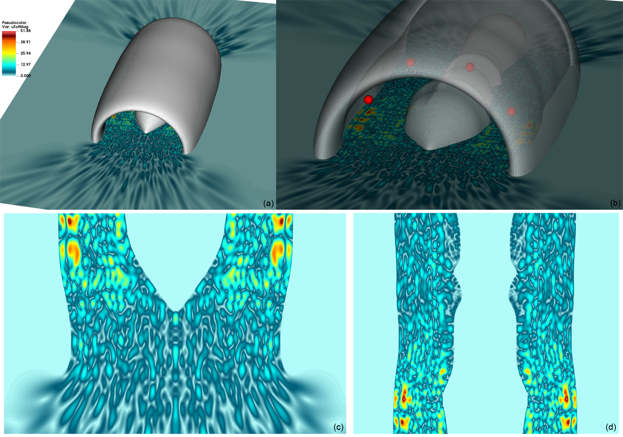
Figure 12: Total field magnitude $|u(x)|=|u^{i}(x)+u^{s}(x)|$ pseudo-color plots for an $82$-wavelength aircraft nacelle. The field is presented over a uniform grid of $2800\times 4000$ points $(x,z)\in[-4,4]\times[-5,6]$. The nacelle is aligned with the $z$-axis and its front points towards the positive $z$-direction. The incident field is given by the sum (73) of eight point sources within the nacelle around the center shaft, four of which are displayed as small red spheres in panel (b).

Near fields resulting for the eight-point source/$81.8\lambda$ problem are presented in Figure 12. The total field magnitude is presented over the $xz$-planar grid $\mathbb{P}_{N}^{xz}(y^{0})$ used previously in this section. Figure 12(a) presents the fields resulting under point-source incidence; note from this image that the resulting fields scatter and exit the front inlet and rear exhaust. The close-up view in Figure 12(b) highlights the location of four of the eight point sources, drawn as red spheres for emphasis; the remaining four sources are obstructed from view by the near field plane. In Figures(c) and (d) the geometry is not included, enabling examination the field interaction within the scatterer in greater detail. These two images exhibit complex multiple scattering and, as mentioned in the context of the plane-wave incidence problem considered earlier in this section, a high degree of symmetry throughout the interior of the structure and in the regions outside that surround the nacelle assembly. In contrast to the plane wave scattering case, where the incident wave travels in directions mostly parallel to the housing and shaft, placing sources between the shaft and nacelle walls guarantees that most waves are scattered many times by the surface before exiting the geometry.

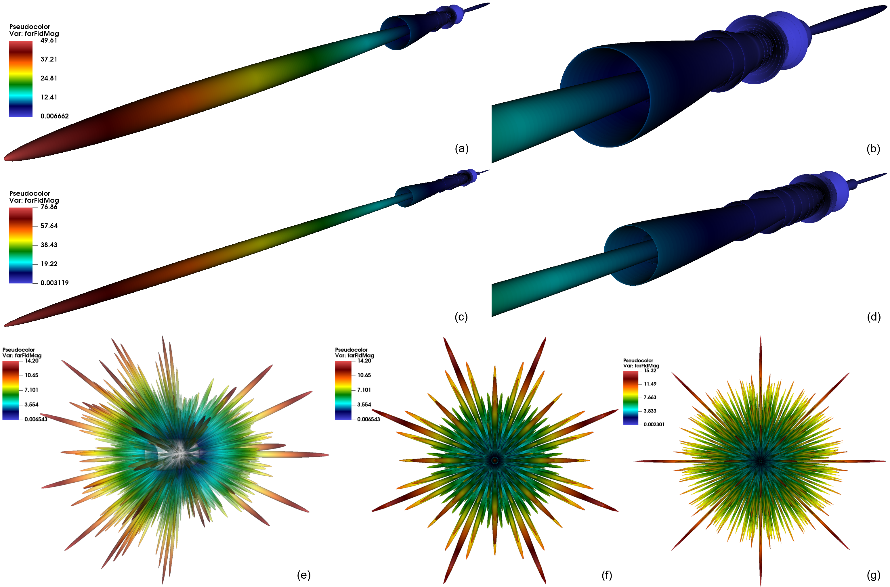
Figure 13: Far-field magnitudes for the nacelle geometry under plane wave and eight point-source incident fields. Panels (a) and (b) present the far field for a $40.9\lambda$ plane wave and panels (c) and (d) present the far field for an $81.8$-wavelength plane wave. Panels (e)-(g) display far fields for the eight-point source incident field defined in (73), for $40.9\lambda$ in panels (e) and (f) and for $81.8\lambda$ in panel (g).

Figure 13 displays far-field magnitudes for both the plane-wave and multiple-point source problems considered in this section. In detail, Figures 13(a) and 13(b) present the far field for a $40.9\lambda$ plane wave; and Figures 13(c) and 13(d) present the far field for an $81.8$-wavelength plane wave, all of which were computed using the relation (66) over the discrete spherical discretization $\mathbb{S}^{2}_{N}$ (equation (67)) with $(N_{\phi},N_{\theta})=(2000,600)$ in the $40.9\lambda$ case, and with $(N_{\phi},N_{\theta})=(3200,800)$ in the $81.8\lambda$ case. These far field plots once again highlight the fact that most of the wave energy is reflected toward the region directly in front of the nacelle intake; note, also, that this reflection increases in intensity as the frequency increases: the maximum far-field magnitude increases by a factor of approximately $1.5$ as the problem size is increased from $40.9\lambda$ to $81.8\lambda$. Figures 13(e-g) show the far field magnitude for the eight-point source incident field (73) at $40.9$ and $81.8$ wavelengths. Figure 13(e) displays a side view of the $40.9\lambda$ far field magnitude $|\tilde{u}^{\infty}|$ including the nacelle geometry, for reference, with the intake pointing left. Figures 13(f) and 13(g), where the geometry is not included, present the far field, with the positive $z$ direction pointing out of the page, for the $40.9\lambda$ and $81.8\lambda$ cases, respectively.

6 Conclusions

The IFGF/RP scattering solver introduced in this paper demonstrates, for the first time, the character of the IFGF acceleration algorithm in the context of an actual problem of scattering. The combined approach achieves accurate scattering simulations on the basis of an $\mathcal{O}(N\log N)$ computational cost. Without recourse to the FFT algorithm, and relying, instead, on a recursive interpolation scheme, the IFGF accelerator enables the fast evaluation of the slowly-varying factors in the factored Green function representations for groups of sources. The IFGF algorithm is additionally integrated seamlessly with the high-order RP methodology. Two different strategies are proposed in Section 3 for the treatment of the double layer operator, each one of which, for efficiency, is recommended for use under certain portions of the IFGF recursion. The OpenMP implementation reported in this paper delivers accurate results in brief computing times, and with fully converged solutions within the accuracy quoted, even for the relatively large acoustical sizes and for the complex and realistic scattering structures considered. Comparisons with recent FMM-based solvers, presented in Section 5.2, demonstrate the benefits provided by the proposed IFGF/RP approach.

Beyond providing simulations of acoustic scattering by a sphere of up to $128$ wavelengths in diameter, this paper demonstrated the versatility of the proposed algorithms by including computational results for two realistic engineering geometries, a submarine and a turbofan nacelle. The present contribution only considered a shared-memory implementation of acoustic IFGF-based integral equation solvers; the numerical examples presented show that even in this case the proposed algorithm enables the efficient solution of problems with millions of unknowns over complex geometries on the basis of a small computer system. Owing in part to its virtually unique ability to efficiently accelerate scattering operators without recourse to the FFT, the IFGF algorithm can effectively be parallelized under the MPI interface as well [14]—and, thus, we believe the IFGF/RP algorithm could advantageously be implemented in distributed-memory systems. The development of such a MPI/OpenMP parallel IFGF/RP implementation, which lies beyond the scope of this paper, is left for future work.

CRediT authorship contribution statement

Oscar P. Bruno: Conceptualization, Methodology, Validation, Investigation, Resources, Writing, Supervision, Funding acquisition. Edwin Jimenez: Conceptualization, Methodology, Software, Validation, Investigation, Writing, Visualization. Christoph Bauinger: Conceptualization, Methodology, Software, Validation, Investigation, Writing, Visualization.

Declaration of competing interest

The authors declare that they have no known competing financial interests or personal relationships that could have appeared to influence the work reported in this paper.

References

- [1] Youcef Saad and Martin H Schultz. Gmres: A generalized minimal residual algorithm for solving nonsymmetric linear systems. SIAM Journal on scientific and statistical computing, 7(3):856–869, 1986.
- [2] Oscar P Bruno and Emmanuel Garza. A chebyshev-based rectangular-polar integral solver for scattering by geometries described by non-overlapping patches. Journal of Computational Physics, 421:109740, 2020.
- [3] Christoph Bauinger and Oscar P. Bruno. “Interpolated Factored Green Function” method for accelerated solution of scattering problems. Journal of Computational Physics, 430:110095, 2021.
- [4] David Colton and Rainer Kress. Integral equation methods in scattering theory. SIAM, 2013.
- [5] E Bleszynski, M Bleszynski, and T Jaroszewicz. Aim: Adaptive integral method for solving large-scale electromagnetic scattering and radiation problems. Radio Science, 31(5):1225–1251, 1996.
- [6] Oscar P Bruno and Leonid A Kunyansky. A fast, high-order algorithm for the solution of surface scattering problems: basic implementation, tests, and applications. Journal of Computational Physics, 169(1):80–110, 2001.
- [7] Hongwei Cheng, William Y Crutchfield, Zydrunas Gimbutas, Leslie F Greengard, J Frank Ethridge, Jingfang Huang, Vladimir Rokhlin, Norman Yarvin, and Junsheng Zhao. A wideband fast multipole method for the Helmholtz equation in three dimensions. Journal of Computational Physics, 216(1):300–325, 2006.
- [8] Björn Engquist and Lexing Ying. Fast directional multilevel algorithms for oscillatory kernels. SIAM Journal on Scientific Computing, 29(4):1710–1737, 2007.
- [9] Eric Michielssen and Amir Boag. A multilevel matrix decomposition algorithm for analyzing scattering from large structures. IEEE Transactions on Antennas and Propagation, 44(8):1086–1093, 1996.
- [10] Joel R Phillips and Jacob K White. A precorrected-fft method for electrostatic analysis of complicated 3-d structures. IEEE Transactions on Computer-Aided Design of Integrated Circuits and Systems, 16(10):1059–1072, 1997.
- [11] Jack Poulson, Laurent Demanet, Nicholas Maxwell, and Lexing Ying. A parallel butterfly algorithm. SIAM Journal on Scientific Computing, 36(1):C49–C65, 2014.
- [12] Vladimir Rokhlin. Diagonal forms of translation operators for the Helmholtz equation in three dimensions. Applied and computational harmonic analysis, 1(1):82–93, 1993.
- [13] Lexing Ying, George Biros, Denis Zorin, and Harper Langston. A new parallel kernel-independent fast multipole method. In SC’03: Proceedings of the 2003 ACM/IEEE conference on Supercomputing, pages 14–14. IEEE, 2003.
- [14] Christoph Bauinger and Oscar P. Bruno. Massively parallelized Interpolated Factored Green Function method. In revision; available at https://arxiv.org/abs/2112.15198v2, 2022.
- [15] Roger F Harrington. Field computation by moment methods. IEEE Press, 1992.
- [16] Matt Wala and Andreas Klöckner. A fast algorithm for quadrature by expansion in three dimensions. Journal of Computational Physics, 388:655–689, 2019.
- [17] Mustafa Abduljabbar, Mohammed Al Farhan, Noha Al-Harthi, Rui Chen, Rio Yokota, Hakan Bagci, and David Keyes. Extreme scale fmm-accelerated boundary integral equation solver for wave scattering. SIAM Journal on Scientific Computing, 41(3):C245–C268, 2019.
- [18] M.S. Warren and J.K. Salmon. A parallel hashed oct-tree n-body algorithm. In Supercomputing ’93:Proceedings of the 1993 ACM/IEEE Conference on Supercomputing, pages 12–21, 1993.
- [19] Caleb Waltz, Kubilay Sertel, Michael A. Carr, Brian C. Usner, and John L. Volakis. Massively parallel fast multipole method solutions of large electromagnetic scattering problems. IEEE Transactions on Antennas and Propagation, 55(6):1810–1816, 2007.
- [20] Björn Engquist and Lexing Ying. Fast directional multilevel algorithms for oscillatory kernels. SIAM Journal on Scientific Computing, 29(4):1710–1737, 2007.
- [21] Austin R. Benson, Jack Poulson, Kenneth Tran, Björn Engquist, and Lexing Ying. A parallel directional fast multipole method. SIAM Journal on Scientific Computing, 36(4):C335–C352, 2014.
- [22] David Colton and Rainer Kress. Inverse Acoustic and Electromagnetic Scattering Theory, Third Edition. Applied mathematical sciences. Springer-Verlag, 2013.
- [23] Hank Childs, Eric Brugger, Brad Whitlock, Jeremy Meredith, Sean Ahern, David Pugmire, Kathleen Biagas, Mark Miller, Cyrus Harrison, Gunther H. Weber, Hari Krishnan, Thomas Fogal, Allen Sanderson, Christoph Garth, E. Wes Bethel, David Camp, Oliver Rübel, Marc Durant, Jean M. Favre, and Paul Navrátil. VisIt: An End-User Tool For Visualizing and Analyzing Very Large Data. In High Performance Visualization–Enabling Extreme-Scale Scientific Insight, pages 357–372. Oct 2012.
- [24] J. J. Bowman, T. B. A. Senior, and P. L. E. Uslenghi. Electromagnetic and Acoustic Scattering by Simple Shapes. CRC Press, 1st edition, 1988.
- [25] Christopher W Nell and Layton E Gilroy. An improved basis model for the betssi submarine. DRDC Atlantic TR, 199:2003, 2003.
- [26] Hans G Schneider, R Berg, L Gilroy, I Karasalo, I MacGillivray, MT Morshuizen, and A Volker. Acoustic scattering by a submarine: Results from a benchmark target strength simulation workshop. ICSV10, pages 2475–2482, 2003.
- [27] Sascha Merz, Roger Kinns, and Nicole Kessissoglou. Structural and acoustic responses of a submarine hull due to propeller forces. Journal of sound and vibration, 325(1-2):266–286, 2009.
- [28] Ilkka Karasalo. Modelling of acoustic scattering from a submarine. In Proceedings of Meetings on Acoustics ECUA2012, volume 17, page 070017. Acoustical Society of America, 2012.
- [29] Yingsan Wei, Yang Shen, Shuanbao Jin, Pengfei Hu, Rensheng Lan, Shuangjiang Zhuang, and Dezhi Liu. Scattering effect of submarine hull on propeller non-cavitation noise. Journal of sound and vibration, 370:319–335, 2016.
- [30] C Testa and L Greco. Prediction of submarine scattered noise by the acoustic analogy. Journal of Sound and Vibration, 426:186–218, 2018.
- [31] Jon Vegard Venås and Trond Kvamsdal. Isogeometric boundary element method for acoustic scattering by a submarine. Computer Methods in Applied Mechanics and Engineering, 359:112670, 2020.
- [32] Ali H Nayfeh, John E Kaiser, and Demetri P Telionis. Acoustics of aircraft engine-duct systems. AIAA Journal, 13(2):130–153, 1975.
- [33] Walter Eversman. Theoretical models for duct acoustic propagation and radiation. NASA. Langley Research Center, Aeroacoustics of Flight Vehicles: Theory and Practice. Volume 2: Noise Control, 1991.
- [34] D Casalino, F Diozzi, R Sannino, and A Paonessa. Aircraft noise reduction technologies: a bibliographic review. Aerospace Science and Technology, 12(1):1–17, 2008.
- [35] Matthew Fergus Kewin. Acoustic liner optimisation and noise propagation through turbofan engine intake ducts. PhD thesis, University of Southampton, 2013.
- [36] KR Pyatunin, NV Arkharova, and AE Remizov. Noise simulation of aircraft engine fans by the boundary element method. acoustical physics, 62(4):495–504, 2016.
- [37] MSC Software. Customer Case Studies 2021-04-27; Case Study: Airbus: Simulation helps airbus optimize acoustic liners and reduce aircraft noise, 2021. https://files.mscsoftware.com/cdn/farfuture/-WeJrL0uOWa_LL2SdOen2NMogjF1cpQl5PQF07shqyg/mtime:1401395701/sites/default/files/cs_airbus_ltr_w_4.pdf, last checked on 2021-10-14.