Isovector density and isospin impurity in ${}^{40}\mathrm{Ca}$

Abstract

We study isoscalar (IS) and isovector (IV) densities in ${}^{40}\mathrm{Ca}$ in comparison with theoretical densities calculated by Skyrme Hatree-Fock (HF) models. The charge symmetry breaking and the charge independence breaking forces are introduced to study the effect on the IV density. The effect of isospin mixing in the ground-state density is examined by using the particle-vibration coupling model taking into account the collective IV giant monopole excitation. We show a clear correlations in the IV density and isospin impurity of ${}^{40}\mathrm{Ca}$ within the HF and the particle-vibration coupling model. We extract for the first time the experimental information of isospin impurity from the magnitude of IV density.

1 Introduction

Experimental charge densities have been studied by electron scattering experiments from 1950s. Proton densities can be extracted from the charge densities removing the proton finite-size effect. It has been shown in Refs. [1, 2, 3] that the proton elastic scattering is quite useful to extract the matter distributions of nuclear ground states. Combining the proton and the matter density distributions, the neutron density can be extracted from the experimental data. The neutron density distributions and neutron-skin thicknesses, $\Delta r_{np}$, in ${}^{40}\mathrm{Ca}$ and ${}^{48}\mathrm{Ca}$ are recently determined from the angular distributions of the cross sections and the analyzing powers of polarized proton elastic scattering at $E_{p}=295\,\mathrm{MeV}$ [2]. Experimental proton and neutron rms radii are listed for ${}^{40}\mathrm{Ca}$ and ${}^{48}\mathrm{Ca}$ in Table 1 together with those of ${}^{208}\mathrm{Pb}$. The determination of the proton and neutron density distributions and $\Delta r_{np}$ of ${}^{48}\mathrm{Ca}$ gives a unique opportunity to examine more comprehensively nuclear and neutron matter EoS at various densities [4].

The Skyrme HF model is one of the most successful mean-field models to describe the ground-state properties including single-particle energy spectra of closed-shell and open-shell nuclei. These models are applied also to describe excited states such as low-lying collective states and giant resonances. The Skyrme interactions were originally determined by fitting charge radii and masses of closed shell nuclei, while some parameter sets were optimized including the nuclear matter incompressibility, the Landau-Migdal parameters and/or the neutron matter EoS in the input data. While these effective interactions can reproduce the saturation properties of symmetric nuclear matter well, they have generally different isoscalar and isovector nuclear matter properties. We use hereafter modern version of energy density functions (EDFs) [5]; SAMi-J family as Skyrme EDFs for the study of IS and IV densities.

The charge symmetry breaking (CSB) and charge independence breaking (CIB) forces have been discussed in the context of isospin impurity effect on the super-allowed Fermi decays. The quantitative information of isospin symmetry breaking (ISB) forces is recently examined to calculate the binding energies of isodoublet and isotriplet nuclei [6] and also the excitation energies of isobaric analogue states (IAS) [7]. The ISB interactions are not included in the standard Skyrme EDFs. In this paper, we introduce the Skyrme-type ISB interactions and study how the IV density in a $N=Z$ nucleus ${}^{40}\mathrm{Ca}$ is affected by these interactions. Furthermore, we will extract the correlation between IV density and the isospin impurity through the ISB forces. The IV density is also examined by using the particle-vibration coupling (PVC) model taking into account the IV giant monopole resonance, which will be useful to relate between the isospin impurity and the IV density.

Table 1: Table of empirical rms radii and neutron-skin thicknesses. $r_{\mathrm{ch}}$ and $r_{p}$, and the extracted $r_{n}$ and $\Delta r_{np}$ in ${}^{40}\mathrm{Ca}$, ${}^{48}\mathrm{Ca}$ and ${}^{208}\mathrm{Pb}$ are listed. Experimental data are taken from Refs. [2, 3, 8]. All data are written in unit of fm.

	Exp.	$r_{\mathrm{ch}}$	$r_{p}$	$r_{n}$	$\Delta r_{np}$
${}^{40}\mathrm{Ca}$	Ref. [2, 8]	$3.480$	$3.385$	$3.375$	$-0.010$
${}^{48}\mathrm{Ca}$	Ref. [2, 8]	$3.460$	$3.387$	$3.555$	$0.168$
${}^{208}\mathrm{Pb}$	Ref. [3, 8]	$5.503$	$5.442$	$5.653$	$0.211$

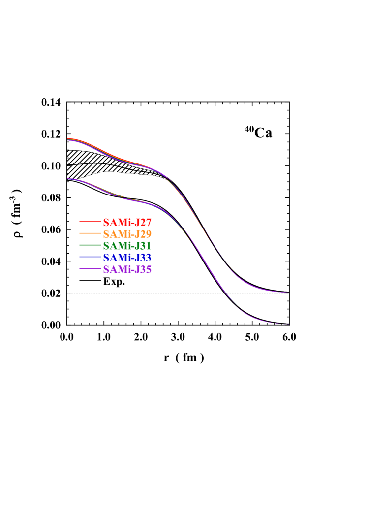
Figure 1: (color online) Experimental proton and neutron densities of ${}^{40}\mathrm{Ca}$ together with calculated ones using SAMi-J interactions. For a guide to eyes, the neutron density is shifted by 0.02 fm^-3. The black solid lines show experimental data taken from Ref. [8] for protons and from Ref. [2] for neutrons. The shaded area of experimental neutron density shows experimental uncertainties of statistical and systematic errors.

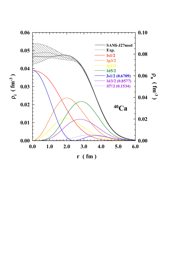
Figure 2: (color online) Calculated neutron density of ${}^{40}\mathrm{Ca}$ with modified occupation probabilities of orbits around the Fermi energy. The contribution of each orbit $\rho_{i}$ with a modified occupation probability, $v_{i}^{2}$, (written in the bracket) for the neutron density is shown with different color. The modified neutron density is denoted as SAMi-J27mod. The orbits without occupation probabilities are fully occupied. See the text for details.

2 Density distributions of ${}^{40}\mathrm{Ca}$

Experimental neutron and proton densities of ${}^{40}\mathrm{Ca}$ are shown in Fig. 1 together with HF results using SAMi-J families. For a guide to eyes, the neutron density is plotted shifting upwards by a unit of 0.02 fm^-3. Experimental proton density is deduced from the charge density observed by electron scattering subtracting the contribution of finite proton size [8, 2]. The observed neutron density has a large uncertainty as shown by a shaded area in these figures, while the proton density is better determined experimentally with a small uncertainty. It is clear that the determination of density distribution is more uncertain in the interior region compared with the surface region.

In Fig. 1, we can see a small variation in the calculated densities depending on different SAMi-J interactions. The SAMi-J family has a variation in the symmetry energy coefficient $J$ from $27$ to $35\,\mathrm{MeV}$ as well as other symmetry energy coefficients $L$ and $K_{\mathrm{sym}}$. Calculated nuclear matter properties and rms radii by SAMi-J families are listed in the supplemental materials. In general, the SAMI-J model underpredicts both proton and neutron densities at around a half of the saturation density near $r\simeq 3.0\,\mathrm{fm}$, while the model overpredicts in the interior region $0\,\mathrm{fm}\leq r\leq 3(1.5)\,\mathrm{fm}$ for neutrons (protons). In Fig. 1, there are small, but systematic differences in the neutron-skin $\Delta r_{np}$ as listed in Table 1 in the supplemental materials: a smaller $J$ value as well as $L$ value produces a larger negative neutron-skin. The calculated results of relativistic mean field model with DDME-J Lagrangians are also shown in the supplemental materials. General features of calculated results are quite similar to those of the Skyrme model, but the deviations of calculated results from empirical data are somewhat larger than those of the Skyrme models.

Figure 2 shows the calculated neutron density of ${}^{40}\mathrm{Ca}$ with modified occupation probabilities of orbits around the Fermi energy. In the HF calculations, all $sd$-shell orbits are fully occupied, but the $f$-shell orbits are empty. In Fig. 2, the occupation probabilities of $2s_{1/2}$ orbit and $1d_{3/2}$ orbit are reduced to be 0.67 and 0.86, respectively, while that for $1f_{7/2}$ orbit is increased to be 0.15. The modification is rather arbitrary, but intended to decrease the central part of density and to increase the surface region. In Fig. 2, as on purpose, the agreement between the experimental and calculated densities becomes better than that in Fig. 1, where one can see a clear difference between the experiment and the calculations in the interior part of the density. This phenomenological approach tells us that the correlations beyond the mean field might be manifested in the neutron density, especially in the interior part of nucleus.

Large scale shell model calculations have been performed including the $pf$-shell model configurations in ⁴⁰Ca (see the supplemental materials for details). We calculate also the particle occupation numbers in $sd$-$pf$ shell orbits including full two major shell configurations. We found that the summed occupation numbers $\sum_{j=p,f}(2j+1)v_{i}^{2}$ in $pf$-shell to be 0.7 including up to 4-particle-4-hole configurations from the $sd$-shell closed core. This value is consistent with the experimental analysis of proton transfer reactions on ⁴⁰Ca [9]. In Fig. 2, the occupation number of $2s_{1/2}$ orbit is crucial to decrease the central part of neutron density. The empirical value from Fig. 2 is $(2j+1)v_{i}^{2}=1.34$, which is smaller than the present shell model value 1.85. A smaller particle occupation number for $2s_{1/2}$, 1.7, was suggested also in the experimental analysis of Ref. [9]. On the contrary, the occupation number of $1f_{7/2}$ orbit is large as 1.2 in Fig. 2, while the shell models give about 0.7. The small occupation probability of $2s_{1/2}$ is an interesting open question to be addressed in future study.

In Fig. 3, the isovector density defined by a difference between the neutron and proton densities as $\rho_{\rm IV}=\rho_{n}-\rho_{p}$ is plotted multiplied by a phase space factor $4\pi r^{2}$. In spite of the overall success of the mean field theories in reproduction of experimental neutron and proton densities, the theoretical predictions of the isovector density are qualitatively different from the experimental one: the experimental result of the isovector density has a peak at around $r\sim 3.2$ fm, while the HF model with SAMi-J27 interaction predicts a peak at $r\sim$2.5 fm with positive values (neutron excess) in the interior and negative values (proton excess) at the surface region. The theoretical predictions can be intuitively understood as swelling of the proton distribution due to the repulsive Coulomb force. In the following section, we will theoretically investigate the behavior of the isovector density from a viewpoint of the isospin impurity in a nucleus.

3 A particle-vibration coupling model and IV density

The isospin impurity can be evaluated by using HF, and PVC models to IV giant monopole resonance (GMR). We will adopt hereafter the PVC model to illustrate analytically the connection between the isospin impurity and the IV density. In the PVC model for the evaluation of isospin impurity, the ground state is calculated firstly without the Coulomb and ISB interactions. Then the ISB forces are introduced by the first-order perturbation as

$$\left|{\widetilde{\rm GS}}\right\rangle\simeq\left|{{\rm GS}}\right\rangle+\varepsilon^{\tau=1}\left|{{\rm GMR,\tau=1}}\right\rangle,$$ (1)

taking into account the coupling between the ground state and the collective IV GMR. Here, $\tau=1$ denotes the IV GMR. The coefficient $\varepsilon^{\tau=1}$ of the perturbed state is calculated as

$$\varepsilon^{\tau=1}=\frac{\left\langle{\rm GMR,\tau=1}\middle|{V^{\rm ISB}}\middle|{\rm GS}\right\rangle}{\Delta E^{\tau=1}},$$ (2)

where the energy difference in the denominator is given by $\Delta E^{\tau=1}=E_{\rm GS}-E_{\rm GMR}^{\tau=1}$ for the IVGMR. In the numerator, $V^{\rm ISB}$ is the isospin symmetry breaking interactions.

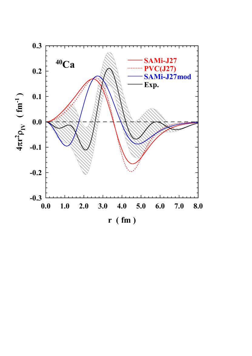
Figure 3: (color online) IV densities multiplied by a factor $4\pi r^{2}\rho_{\rm IV}$ of ${}^{40}\mathrm{Ca}$ calculated by HF, modified HF and PVC models as well as the experimental IV density. The red (blue) solid and dashed curves show the HF (modified HF) and PVC densities with SAMi-J27 (SAMi-J27mod) model, respectively. The experimental data are shown with a black solid curve with the experimental uncertainty shown by the shaded area. The experimental data is taken from Ref. [2], while the calculated densities are obtained by using the HF and modified ground state densities denoted SAMi-J27 and SAMi-J27mod in Figs. 1 and 2, respectively. See the text for details.

The perturbed IV density for the ground state is then expressed as

$$\left\langle{\widetilde{\rm GS}}\middle|{\hat{\rho}_{\rm IV}({\bf r})}\middle|{\widetilde{\rm GS}}\right\rangle$$

$$=\left\langle{\rm GS}\middle|{\hat{\rho}_{\rm IV}({\bf r})}\middle|{\rm GS}\right\rangle+2\varepsilon^{\tau=1}\left\langle{{\rm GMR},\tau=1}\middle|{\hat{\rho}_{\rm IV}({\bf r})}\middle|{\rm GS}\right\rangle$$

$$=\rho_{\rm IV}(r)+2\varepsilon^{\tau=1}\rho^{\rm IVTR}_{\tau=1}({\bf r})\equiv\rho_{\rm IV}(r)+\Delta\rho^{\tau=1}_{\rm IVTR},$$ (3)

where the IV density operator reads $\hat{\rho}_{\rm IV}({\bf r})=\sum_{i}\delta({\bf r}-{\bf r}_{i})\tau_{z}(i)$ and $\rho^{\rm IVTR}_{\tau}({\bf r})$ is the transition density defined by

$$\rho^{\rm IVTR}_{\tau=1}({\bf r})\equiv\left\langle{{\rm GMR},\tau=1}\middle|{\hat{\rho}_{\rm IV}({\bf r})}\middle|{{\rm GS}}\right\rangle.$$ (4)

Notice that the first term of Eq. (3) disappears for $N=Z$ nuclei without the ISB interactions. Under the assumption that one collective IV GMR exhausts fully the sum rule strength, the GMR transition density is expressed by the Werntz-Überall type [10],

$$\rho_{\tau=1}^{\rm IVTR}({\bf r})=\alpha^{\tau=1}\rho^{\rm WU}_{\rm tr}\equiv\alpha^{\tau=1}\frac{1}{r^{2}}\frac{d}{dr}\left(r^{3}\rho_{\rm IS}(r)\right)Y_{00}(\hat{r}).$$ (5)

where the amplitude $\alpha^{\tau=1}$ determines the collectiveness of the GMR excitation, $\rho_{\rm IS}(r)$ is the IS ground state density for the operator $\hat{\rho}_{\rm IS}({\bf r})=\sum_{i}\delta({\bf r}-{\bf r}_{i})$, and $Y_{00}(\hat{r})$ is the spherical harmonics with the multipole $\lambda=0$. A similar radial form of transition density is obtained by a hydrodynamical model of compressive irrotational fluid [12]. The collective parameter $\alpha^{\tau=1}$ is normalized to satisfy the energy-weighted sum rule (EWSR) $m_{1}$ for the IVGMR,

$$m_{1}^{\tau=1} \equiv \sum_{n}\hbar\omega^{\tau=1}_{n}\left|\left\langle{n,\tau=1}\middle|{\hat{O}_{\tau=1}^{\lambda=0}}\middle|{{\rm GS}}\right\rangle\right|^{2}$$ (6)

$$= \frac{2\hbar^{2}}{m}\frac{A}{4\pi}\left\langle{r^{2}}\right\rangle_{m},$$

where the monopole transition operator is given by

$$\hat{O}_{\tau=1}^{\lambda=0}=\sum_{i}r_{i}^{2}Y_{00}(\hat{r})\tau_{z}(i).$$ (7)

In Eq. (6), $\left\langle{r^{2}}\right\rangle_{m}$ is the matter mean square radius and $\hbar\omega^{\tau=1}_{n}=E^{\tau=1}_{n}-E_{\rm GS}$. The enhancement of the sum rule by exchange interactions for the IV excitation is neglected in Eq. (6). The IV EWSR is also expressed by using the transition density as

$$m_{1}^{\tau=1}=\hbar\omega_{\rm GMR}^{\tau=1}\left|\alpha^{\tau=1}\right|^{2}\left|\int\rho^{\rm WU}_{\rm tr}r^{4}\,dr\right|^{2}=\hbar\omega_{\rm GMR}^{\tau=1}\left|\alpha^{\tau=1}\right|^{2}\frac{A^{2}}{4\pi^{2}}\left\langle{r^{2}}\right\rangle_{m}^{2},$$ (8)

where we assume that the single collective IV GMR state exhausts the EWSR having the excitation energy $\hbar\omega_{\rm GMR}^{\tau=1}$. The collective amplitude is then obtained as

$$\left|\alpha^{\tau=1}\right|^{2}=\frac{2\hbar^{2}}{m}\frac{\pi}{\hbar\omega_{\rm GMR}^{\tau=1}A\left\langle{r^{2}}\right\rangle_{m}}=\frac{301.5}{\hbar\omega_{\rm GMR}^{\tau=1}}A^{-5/3},$$ (9)

where the mean square radius is taken as $\left\langle{r^{2}}\right\rangle_{m}=3r_{0}^{2}A^{2/3}/5$ fm² with $r_{0}=1.2$ fm. The effect of PVC of IVGMR on the IV density reads

$$\Delta\rho_{\rm IVTR}^{\tau=1}({\bf r})=2\varepsilon^{\tau=1}\rho^{\rm IVTR}_{\tau=1}({\bf r})=2\varepsilon^{\tau=1}\alpha^{\tau=1}\frac{1}{r^{2}}\frac{d}{dr}\left(r^{3}\rho_{\rm IS}(r)\right)\frac{1}{\sqrt{4\pi}}.$$ (10)

4 Isospin impurity and isospin symmetry breaking forces

In the study of isospin impurity of nuclear ground state, the coupling of IVGMR was introduced to evaluate the isospin impurity in the unperturbed ground state with the good isospin [11]. The IVGMR is mixed by the isospin symmetry breaking interaction $V^{\rm ISB}$ as written in Eq. (1). In the following, we consider only the Coulomb force to break the isospin symmetry. The effect of CSB and CIB interactions will be also discussed later.

The mixing amplitude $\varepsilon^{\tau=1}$ might be evaluated with the Coulomb potential,

$$V_{C}(r)=\frac{Ze^{2}}{R}\left(\frac{3}{2}-\frac{r^{2}}{2R^{2}}\right),$$ (11)

which is obtained by assuming a constant charge distribution in the sphere of radius $R$. The mixing matrix element is then expressed as

$$\left\langle{\rm GMR,\tau=1}\middle|{V^{\rm ISB}}\middle|{\rm GS}\right\rangle=\int d{\bf r}\rho^{\rm IVTR}_{\tau=1}({\bf r})V_{C}(r)$$ (12)

In the proton-neutron two-fluid model [12], the excitation energy of IVGMR is estimated to be

$$\hbar\omega^{\tau=1}_{\rm GMR}=170/A^{1/3}\,\mathrm{MeV},$$ (13)

which is 49.7MeV for ${}^{40}\mathrm{Ca}$. Taking the Werntz-Überall-type transition density for IVGMR having the full sum rule strength and the IVGMS energy (13), the isospin impurity is evaluated as

$$\varepsilon^{2}=2.5\times 10^{-6}Z^{4}/A^{4/3},$$ (14)

which gives $\varepsilon^{2}$=0.29% for ${}^{40}\mathrm{Ca}$. This value is about two times larger than the hydrodynamical model evaluation in Ref. [13], $\varepsilon$ (two-fluid)${}^{2}=3.50\times 10^{-7}Z^{2}A^{2/3}$. The self-consistent RPA calculations for IVGMR were performed in Ref. [14] with Skyrme interactions. With a Skyrme interaction SIII, the IV monopole strength is rather widely spread in energy and the average excitation energy in ${}^{40}\mathrm{Ca}$ becomes a much lower energy, $\overline{\hbar\omega}^{\tau=1}=33.5\,\mathrm{MeV}$, than Eq. (13). Consequently, the microscopic HF+RPA model gives even larger isospin mixing than that given in Eq. (14). In Ref. [15], the isospin impurity is estimated as 0.57 % in ${}^{40}\mathrm{Ca}$ by using HF+TDA model with SIII Skyrme interaction. The sum rule value of Fermi transitions is linked to the isospin impurity in the HF+TDA model, while the present HF model calculates directly the overlap between the proton and neutron HF wave functions to evaluate the isospin impurity. The two models are equivalent to evaluate the impurity, while the HF+RPA model provides an additional effect of the ground state correlations on the isospin impurity.

For the collective amplitude of IVGMR in ${}^{40}\mathrm{Ca}$, Eq. (9) gives $|\alpha^{\tau=1}|^{2}=0.0192$ for the IVGMR energy with SIII interaction. With these $\alpha^{\tau=1}$ and $\varepsilon$, the renormalized transition density gives the IV density in the ground state and compared with the HF isovector density in Fig. 3. It is remarkable that the PVC density obtained by using SAMi-J27 interaction follows quite closely the HF IV density. This is the reason why the HF and PVC models give almost the same isospin impurity although the two models evaluate quite differently the values [15, 16]. Thus, the large isospin impurity obtained by the HF results takes into account implicitly the coupling between the single-particle wave functions and the collective IVGMR due to the Coulomb interaction.

The IV density of modified HF results extracted from Fig. 2 is also shown in Fig. 3 as SAMi-J27mod. It is noted that the peak height of SAMi-J27mod is almost the same as those of HF and PVC results. This feature encourages to extract the isospin impurity from the maximum of the experimental IV density, which will be discussed hereafter.

The CSB and CIB interactions were introduced in the context of Skyrme interactions in Refs. [6, 7, 17]. While there are several possible channels in both CSB and CIB interactions, we consider $s$-wave interactions as the main channel,

$$v_{\rm{Sky}}^{\rm{CSB}}\left(\vec{r}\right) =s_{0}\left(1+y_{0}P_{\sigma}\right)\delta\left(\vec{r}\right)\frac{\tau_{z1}+\tau_{z2}}{4},$$ (15a)

$$v_{\rm{Sky}}^{\rm{CIB}}\left(\vec{r}\right) =u_{0}\left(1+z_{0}P_{\sigma}\right)\delta\left(\vec{r}\right)\frac{\tau_{z1}\tau_{z2}}{2}.$$ (15b)

The energy density of ISB part of the Skyrme interaction reads

$$\mathcal{E}_{\rm{CSB}} =\frac{s_{0}\left(1-y_{0}\right)}{8}\left(\rho_{n}^{2}-\rho_{p}^{2}\right),$$ (16a)

$$\mathcal{E}_{\rm{CIB}} =\frac{u_{0}}{8}\left[\left(1-z_{0}\right)\left(\rho_{n}^{2}+\rho_{p}^{2}\right)-2\left(2+z_{0}\right)\rho_{n}\rho_{p}\right].$$ (16b)

The mean-field potentials of CSB and CIB can be evaluated by a functional derivative of energy density with respect to proton and neutron densities;

$$V_{\rm CSB}^{n}(r) =\frac{\delta\mathcal{E}_{\rm{CSB}}}{\delta\rho_{n}}=\frac{s_{0}(1-y_{0})}{4}\rho_{n},$$ (17a)

$$V_{\rm CSB}^{p}(r) =\frac{\delta\mathcal{E}_{\rm{CSB}}}{\delta\rho_{p}}=-\frac{s_{0}(1-y_{0})}{4}\rho_{p},$$ (17b)

and

$$V_{\rm CIB}^{n}(r) =\frac{\delta\mathcal{E}_{\rm{CIB}}}{\delta\rho_{n}}=\frac{u_{0}(1-z_{0})}{4}\rho_{n}-\frac{u_{0}}{4}(2+z_{0})\rho_{p},$$ (18a)

$$V_{\rm CIB}^{p}(r) =\frac{\delta\mathcal{E}_{\rm{CIB}}}{\delta\rho_{p}}=\frac{u_{0}(1-z_{0})}{4}\rho_{p}-\frac{u_{0}}{4}(2+z_{0})\rho_{n}.$$ (18b)

In SAMi-ISB parameter sets [7], the CSB and CIB interactions are optimized for a set of experimental data to be $s_{0}=-26.3\,\mathrm{MeV}\,\mathrm{fm}^{3}$ and $u_{0}=25.8\,\mathrm{MeV}\,\mathrm{fm}^{3}$ for the choice of spin-exchange parts $y_{0}=-1$ and $z_{0}=-1$.

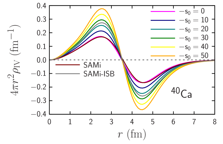
Figure 4: (color online) IV density in ${}^{40}\mathrm{Ca}$ calculated by a HF model with various SAMi parameter sets. The parameter $-s_{0}$ of CSB interaction is varied from $0$ to $50\,\mathrm{MeV}\,\mathrm{fm}^{3}$ with a step of $10\,\mathrm{MeV}\,\mathrm{fm}^{3}$ keeping CIB parameter $u_{0}=0\,\mathrm{MeV}\,\mathrm{fm}^{3}$ on top of the central part of SAMi-ISB parameter set. See the text for details.

We study how much the IV density is changed by different values of ISB interactions in Fig. 4. In Fig. 4, the strength of CSB interaction is varied from $-s_{0}=0$ to $50\,\mathrm{MeV}\,\mathrm{fm}^{3}$ with a step of $10\,\mathrm{MeV}\,\mathrm{fm}^{3}$, keeping CIB parameter $u_{0}=0\,\mathrm{MeV}\,\mathrm{fm}^{3}$, as did in Ref. [18]. It is remarkable that the CSB effect enhances largely the IV density. The CIB parameter dependence is also checked to change $u_{0}=0$, $25$, and $50\,\mathrm{MeV}\,\mathrm{fm}^{3}$ keeping the CSB parameter $-s_{0}=0\,\mathrm{MeV}\,\mathrm{fm}^{3}$ as shown in Fig. 2 of the supplemental materials. We found that the CIB interaction does not change at all the magnitude of IV density in contrast to the results of the change of CSB interaction strength (see for details the supplemental materials).

Figure 5 shows the isospin impurity as a function of $-s_{0}$ ($u_{0}$) for the CSB (CIB) interaction. The value indicated by the arrow with “SAMi” is induced entirely by the Coulomb interaction, while the arrow labelled by “All ISB” is the one by SAMi-ISB. There is a clear difference between the CSB and CIB dependence. Namely, the CIB has no effect on the isospin impurity, while the CSB gives a large enhancement on the isospin impurity. The correlation coefficient between the CSB strength and the isospin impurity is very high as $r=0.991$. Consequently, the parameter set SAMi-ISB gives much larger value than that of SAMi, i.e., more than a factor 2 larger than the SAMi value.

This peculiar feature of CSB and CIB can be understood by studying the mean-field potentials originated by CSB and CIB interactions. Taking $y_{0}=z_{0}=-1$ as is the same as SAMi-ISB [7], the mean-field potential of CSB and CIB interactions are expressed as Eq. (17) shows that the CSB contribution has a pure IV character to enhance the difference between neutron and proton density distributions. On the other hand, the CIB potentials (18) do not give any enhancement on the IV density. The CIB interaction violates in general the isospin invariance characterized by the rotation in the isospin space. However, the CIB interaction holds the charge symmetry due to the isospin rotation by 180^∘ about the $y$-axis [19]. Thus, the characteristic features of CSB and CIB interactions in Figs. 4 and 5 are interpreted as the outcome of the intrinsic nature of CSB and CIB interactions.

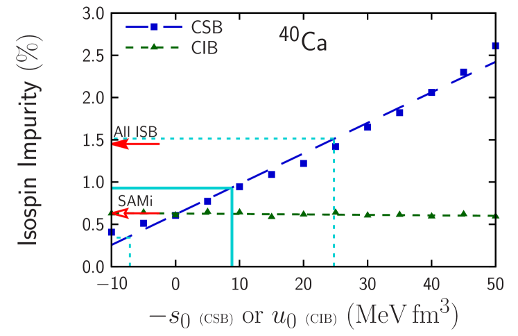
Figure 5: (color online) Isospin impurity in ${}^{40}\mathrm{Ca}$ calculated by a HF model with various strength of CSB and CIB interactions. The strength of CSB, $-s_{0}$, and CIB, $u_{0}$, are varied from $-10$ to $50\,\mathrm{MeV}\,\mathrm{fm}^{3}$ with a step of $5\,\mathrm{MeV}\,\mathrm{fm}^{3}$. The correlation coefficient between two values is $r=0.991$. The parameter set SAMi has no ISB interactions, while SAMi-ISB (denoted All ISB) has the CSB and CIB strength $-s_{0}=26.3\,\mathrm{MeV}\,\mathrm{fm}^{3}$ and $u_{0}=25.8\,\mathrm{MeV}\,\mathrm{fm}^{3}$, respectively. The cyan line is drawn to extract the CSB strength $-s_{0}$ from the isospin impurity determined in Fig. 6. The cyan dashed lines are experimental uncertainty. See the text for details.

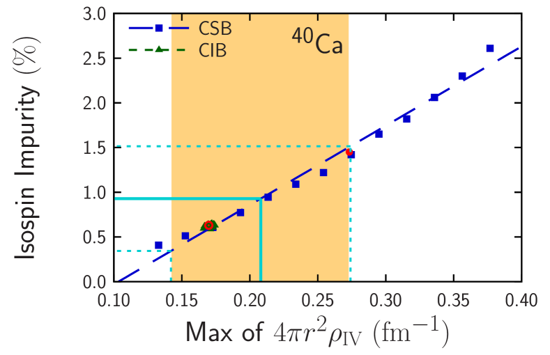
Figure 6: (color online) Isospin impurity vs. the peak of IV density in ${}^{40}\mathrm{Ca}$. The calculations are performed by changing the strength of CSB and CIB interactions on top of the central part of SAMi-ISB parameter set. The correlation coefficient between two values is $r=0.992$. The red circle and the double red circle show the results of SAMi-ISB and SAMi interactions, respectively. The results of CIB interaction are seen as one green triangle since the results are changed scarcely by the change of strength of CIB interaction and overlapped largely in the scale of this figure.

Figure 6 shows the correlation between the maximum of IV density and the isospin impurity. The correlation coefficient is very high as $r=0.992$. This clear correlation is expected from very smooth increase of both the IV density and the isospin impurity in Figs. 4 and 5. It could be possible to extract the isospin impurity from the peak height of IV density when both the proton and neutron densities are available experimentally. The experimental peak height of IV density is shown to be $0.208\pm 0.066$ fm^-1 in Fig. 3. The isospin impurity is then extracted from the correlation plot of Fig. 6 as

$$\varepsilon^{2}=0.928\pm 0.586.$$ (19)

This central value is about 50% larger than the value of RPA calculations without the ISB forces in Ref. [15]. From this value of the isospin impurity, the strength of CSB interaction $s_{0}$ is further obtained as

$$s_{0}=-\left(8.80\pm 16.0\right)\,\mathrm{MeV}\,\mathrm{fm}^{3},$$ (20)

from the correlation plot in Fig. 5.

The calculated results of CSB dependence of isospin impurities in other $N=Z$ nuclei, ⁸⁰Zr and ¹⁰⁰Sn, are shown in Fig. 7. We found again very similar strong CSB dependence of the impurities of ⁸⁰Zr and ¹⁰⁰Sn in these figures, while the CIB interaction does not give any appreciable effect.

It is shown that the correlation between the area of IV density and the isospin impurity is as strong as that between the peak height and the isospin impurity shown in Fig. 6 (see the supplemental materials for details). These features support our procedure to extract the isospin impurity, as well as the CSB strength, from the correlation between the magnitude of IV density and the isospin impurity.

5 Summary and future perspectives

In summary, we studied the IV and IS densities of ${}^{40}\mathrm{Ca}$ by using the mean-field and PVC models. As the mean-field models, we took Skyrme SAMi-J model. We found an appreciable difference between the experimental and calculated IS densities in the interior part and also dilute density region of ${}^{40}\mathrm{Ca}$. This difference suggests the modification of density distribution by reduced occupation probabilities of single-particle states near the Fermi surface, which may be caused by many-body correlations beyond the mean-field model.

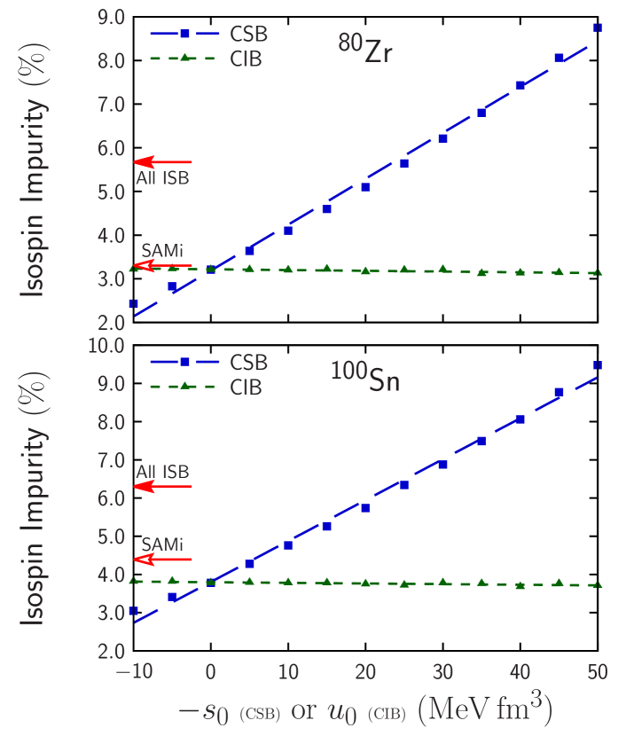
Figure 7: (color online) Isospin impurities in ${}^{80}\mathrm{Zr}$ and ${}^{100}\mathrm{Sn}$ calculated by a HF model with various strength of CSB and CIB interactions on top of the central part of SAMi-ISB interaction. The strength of CSB, $-s_{0}$, and CIB, $u_{0}$, are varied from $-10$ to $50\,\mathrm{MeV}\,\mathrm{fm}^{3}$ with a step of $5\,\mathrm{MeV}\,\mathrm{fm}^{3}$. The correlation coefficient between the isospin impurity and the CSB interaction is $r=0.996$. The parameter set SAMi has no ISB interactions, while SAMi-ISB (denoted All ISB) has the CSB and CIB strength $-s_{0}=26.3\,\mathrm{MeV}\,\mathrm{fm}^{3}$ and $u_{0}=25.8\,\mathrm{MeV}\,\mathrm{fm}^{3}$, respectively.

The IV density is examined in the Skyrme HF model, and also the PVC model taking into account the IV GMR. We found a close resemblance between the HF and PVC IV densities, which will cause the same amount of isospin impurity in the ground state of ${}^{40}\mathrm{Ca}$. It was also shown that the magnitude of IV density is changed largely by the CSB interaction, while the CIB interaction gives no appreciable effect. It is found the CSB interaction shows a strong linear correlation with the maximum of IV density as well as with the isospin impurity. Thus, the magnitude of IV density gives a good clue to determine experimentally the isospin impurity and the magnitude of CSB interaction. This characteristic feature of IV density appear not only in ${}^{40}\mathrm{Ca}$, but also in other $N=Z$ nuclei, ${}^{80}\mathrm{Zr}$ and ${}^{100}\mathrm{Sn}$. Precise measurements of the IV density is desperately desired to obtain experimental information of the isospin impurity and also the CSB interaction.

This work was supported by JSPS KAKENHI Grant Numbers 15H054, JP19K03858, and JP19J20543. We thank M. Honma, N. Shimizu, and T. Fukui for informing us shell model results of ⁴⁰Ca. The numerical calculations were partly performed on cluster computers at the RIKEN iTHEMS program.

References

-
[1]
L. Ray et al., Phys. Rev. C 18, 2641 (1978)
V. E. Starodubsky and N. M. Hintz, Phys. Rev. C 49, 2118 (1994).
S. Terashima et al., Phys. Rev. C 77, 024317 (2008).
H. Sakaguchi and J. Zenihiro, Prog. Part. Nucl. Phys. 97, 1 (2017). - [2] J. Zenihiro et al., arXiv:1810.11796 (2018).
- [3] J. Zenihiro et al., Phys. Rev. C 82, 044611 (2010).
- [4] J. Zenihiro, T. Uesaka, S. Yoshida, and H. Sagawa, Prog. Theo. Exp. Phys. 2021, 023D05 (2021).
- [5] S. Yoshida, H. Sagawa, J. Zenihiro, and T. Uesaka, Phys. Rev. C 102, 064307 (2020).
-
[6]
P. Bączyk and J. Dobaczewski and M. Konieczka and W. Satuła and T. Nakatsukasa and K. Sato,
Phys. Lett. B 778, 178 (2018).
P. Bączyk and W. Satula and J. Dobaczewski and M. Konieczka, J. Phys. G 46, 03LT01 (2019). - [7] X. Roca-Maza, G. Colò, and H. Sagawa, Phys. Rev. Lett. 120, 202501 (2018).
- [8] H. de Vries, C. W. de Jager, and C. de Vries, At. Data Nucl. Data Tables 36, 495 (1987).
-
[9]
P. Doll P, G. J. Wagner, K. T. Knopfle and G. Mairle, Nucl. Phys. A 263 210 (1976).
F. Malaguti, A. Uguzzoni, E. Verondini and P. E. Hodgson, Nucl. Phys. A 297 287 (1978); ibid., Nuovo Cim. A 49 412 (1979). - [10] C. Werntz and H. Überall, Phys. Rev. 149, 762 (1966).
- [11] N. Auerbach, Phys. Rev. C79, 035502 (2009).
- [12] A. Bohr and B. R. Mottelson, Nuclear Structure Vol. II (World Scientific, 1998).
- [13] A. Bohr and B. R. Mottelson, Nuclear Structure Vol. I, p. 173 (World Scientific, 1998).
- [14] I. Hamamoto, H. Sagawa, and X. Z. Zhang, Phys. Rev. C 56, 3121 (1997).
- [15] I. Hamamoto and H. Sagawa, Phys. Rev. C 48 R960 (1993).
- [16] X. Roca-Maza, G. Colò, and H. Sagawa, Phys. Rev. C102. 064303 (2020).
-
[17]
H. Sagawa, N. Van Giai, and T. Suzuki,
Phys. Lett. B 353, 7 (1995).
H. Sagawa, N. Van Giai and T. Suzuki, Phys. Rev. C 53, 2163 (1996). - [18] T. Naito, G. Colò, H. Liang, X. Roca-Maza, and H. Sagawa, Phys. Rev. C105, L021304 (2022)
- [19] G. A. Miller, A. K. Opper and E. J. Stephenson, Annu. Rev. Nucl. Part. Sci. 56, 253 (2006).