Counting ends on shrinkers

Abstract.

In this paper we apply a geometric covering method to study the number of ends on shrinkers. On one hand, we prove that the number of ends on any complete non-compact shrinker is at most polynomial growth with fixed degree. On the other hand, we prove that any complete non-compact shrinker with certain volume comparison condition has finitely many ends. Some special cases of shrinkers are also discussed.

1. Introduction and main results

An $n$-dimensional Riemannian manifold $(M,g)$ is called a gradient shrinking Ricci soliton or shrinker (see [19]) if there exists a smooth function $f$ on $(M,g)$ such that the Ricci curvature Ric and the Hessian of $f$ satisfy

$${\mathrm{Ric}}+\mathrm{Hess}\,f=\lambda g$$

for some constant $\lambda>0$. Function $f$ is often called a potential of the shrinker. Upon scaling the metric $g$ by a constant, we may assume $\lambda=1/2$ so that

$${\mathrm{Ric}}+\mathrm{Hess}\,f=\frac{1}{2}g.$$ (1.1)

Furthermore, we can normalize $f$ such that (1.1) simultaneously satisfies

$$\mathrm{S}+|\nabla f|^{2}-f=0,$$ (1.2)

where $\mathrm{S}$ is the scalar curvature of $(M,g)$, and

$$\int_{M}(4\pi)^{-\frac{n}{2}}e^{-f}dv=e^{\mu},$$ (1.3)

where $dv$ is the volume element with respect to metric $g$, and $\mu=\mu(g,1)$ is the entropy functional of Perelman [37]. By Lemma 2.5 in [26], we see that the term $e^{\mu}$ is almost equivalent to the volume of geodesic ball $B(p,1)$ with radius $1$ and center $p$. Here $p\in M$ is a infimum point of $f$, which can be always achieved for any complete shrinker; see [20].

Shrinkers play an important role in the Ricci flow as they correspond to some self-similar solutions and usually arise as the limit solutions of type I singularity models of the Ricci flow [15]. They are regarded as a natural extension of Einstein manifolds with positive scalar curvature, and are related to the Bakry-Émery Ricci tensor [2]. Nowadays, the understanding of geometry and topology for shrinkers is an important subject in the Ricci flow [19]. For dimensions 2 and 3, the classification of shrinkers is complete. However dimensions equal to or greater than 4, the complete classification remains open; see [4, 5] and references therein for nice surveys.

It is an interesting phenomenon that many geometric and analytic properties of shrinkers are similar to manifolds with nonnegative Ricci curvature or Einstein manifolds with positive scalar curvature. Some interesting results are exhibited as follows. Wylie [46] proved that any complete shrinker has finite fundamental group (the compact case due to Derdziński [14]). Fang, Man and Zhang [16] showed that any non-compact shrinker with bounded scalar curvature has finite topological type. Chen and Zhou [6] confirmed that any non-compact shrinker has at most Euclidean volume growth. Munteanu and Wang [34] proved that any non-compact shrinker has at least linear volume growth.

Haslhofer and Müller [20, 21] proved a Cheeger-Gromov compactness theorem of shrinkers with a lower bound on their entropy and a local integral Riemann bound. Li, Li and Wang [26] gave a structure theory for non-collapsed shrinkers, which was further developed by Huang, Li and Wang [23]. For the $4$-dimensional case, Li and Wang [31] proved that any nontrivial flat cone cannot be approximated by smooth shrinkers with bounded scalar curvature and Harnack inequality under the pointed-Gromov-Hausdorff topology. Huang [22] applied the strategy of Cheeger-Tian [9] in Einstein manifolds and proved an $\epsilon$-regularity theorem for $4$-dimensional shrinkers, confirming a conjecture of Cheeger-Tian [9].

Recently, Li and Wang [32] obtained a sharp logarithmic Sobolev inequality, the Sobolev inequality, heat kernel estimates, the no-local-collapsing theorem, the pseudo-locality theorem, etc. on complete shrinkers, which can be further extended to the other geometric inequalities, such as Nash inequalities, Faber-Krahn inequalities and Rozenblum-Cwikel-Lieb inequalities in [43]. For more function theory on shrinkers, the interested readers are referred to [18, 33, 35, 36, 40, 44, 45] and references therein.

On a manifold $M$, a set $E$ is called an end with respect to a compact set $\Omega\subset M$, if it is an unbounded connected component of $M\backslash\Omega$. The number of ends with respect to $\Omega$, denoted by $N_{\Omega}(M)$, is the number of unbounded connected components of $M\backslash\Omega$. If $\Omega_{1}\subset\Omega_{2}$, then $N_{\Omega_{1}}(M)\leq N_{\Omega_{2}}(M)$. Hence if $\Omega_{i}$ is a compact exhaustion of $M$, then $N_{\Omega_{i}}(M)$ is a nondecreasing sequence. If this sequence is bounded, then we say that $M$ has finitely many ends. In this case, the number of ends of $M$ is defined by

$$N(M)=\lim_{i\to\infty}N_{\Omega_{i}}(M).$$

Obviously, the number of ends is independent of the compact exhaustion $\{\Omega_{i}\}$. Ends of manifolds are related to the geometry and topology of manifolds; the interested reader may refer to the book [27].

The Cheeger-Gromoll’s splitting theorem [8] indicates that any complete non-compact manifold with nonnegative Ricci curvature has at most two ends. Later, Cai [3] and Li-Tam [28] independently proved that any manifold with nonnegative Ricci curvature outside a compact set has at most finitely many ends (see also Liu [25]); see [41] for an extension to smooth metric measure spaces. Cai’s approach is pure geometrical, strongly depending on a local version of Cheeger-Gromoll’s splitting theorem, while Li-Tam’s proof is analytic in nature by taking full advantage of the harmonic function theory. Liu’s proof is also geometrical, not adapting the local splitting theorem but using various volume comparisons. At present, an interesting question of whether the Cheeger-Gromoll splitting theorem holds on any complete non-compact shrinker still remains unresolved. In the next attempt to consider the number of ends, it is natural to ask

Question. Does any a complete non-compact shrinker have finitely many ends?

For the Kähler case, Munteanu and Wang [36] proved that any Kähler shrinker has only one end. For the Riemannian case, Munteanu, Schulze and Wang [33] showed that the number of ends is finite when the scalar curvature satisfies certain scalar curvature integral at infinity. Their proof depends on the Li-Tam’s analytic theory [28]. In this paper, we use a geometric covering argument and prove that

Theorem 1.1.

The number of ends on $n$-dimensional complete non-compact shrinker with the scalar curvature

$$\mathrm{S}\geq\delta$$

for some constant $\delta\geq 0$ is at most polynomial growth with degree $2(n-\delta)$.

Remark 1.2.

From (2.8) in Section 2, we will see that $\mathrm{S}\geq\delta$ implies $\delta\leq n/2$ on shrinkers. From Remark 2.6, we have that the point-wise assumption $\mathrm{S}\geq\delta$ can be replaced by a lower of the average scalar curvature over the level set $\{f<r\}:=\left\{x\in M|f(x)<r\right\}$ for any $r>0$, that is,

$$\frac{1}{\int_{\{f<r\}}dv}\int_{\{f<r\}}\mathrm{S}\,dv\geq\delta$$

for any $r>0$. If the scalar curvature also has a uniformly upper bound, then the degree $2(n-\delta)$ in theorem can be reduced to $n-2\delta$; see Remark 3.4.

The following condition introduced in [29] will play an important role in this paper.

Definition 1.3.

A Riemannian manifold $(M,g)$ has volume comparison condition if there exists a constant $\eta>0$ such that for all $r\geq r_{0}$ for some $r_{0}>0$, and all $x\in\partial B(q,r)$,

$$\mathrm{Vol}(B(q,r))\leq\eta\,\mathrm{Vol}\left(B(x,\frac{r}{16})\right),$$

where $\mathrm{Vol}(B(q,r))$ is the volume of geodesic ball $B(q,r)$ of radius $r$ with center at a fixed point $q\in M$.

If the shrinker satisfies volume comparison condition, we prove that

Theorem 1.4.

Any complete non-compact shrinker with volume comparison condition must have finitely many ends.

Many special cases of shrinkers satisfy volume comparison condition. The detailed discussion can be referred to Section 4. Here we summarize some results as follows:

(I) If a manifold satisfies volume doubling property, then it admits volume comparison condition; see Proposition 4.2. Recall that $(M,g)$ is said to be volume doubling property if

$$\mathrm{Vol}(B(x,2r))\leq D\,\mathrm{Vol}(B(x,r))$$

for any $x\in M$ and $r>0$, where $D$ is a fixed constant. Clearly, any manifold with nonnegative Ricci curvature satisfies volume doubling property.

(II) If the asymptotic scalar curvature ratio of shrinker is finite, then such shrinker has volume comparison condition; see Proposition 4.3. Given a point $q\in(M,g)$, the asymptotic scalar curvature ratio ($\operatorname{ASCR}$) is defined by

$$\operatorname{ASCR}(g):=\underset{r(q,x)\to\infty}{\lim\sup}\,\mathrm{S}(x)\cdot r(q,x)^{2},$$

$r(q,x)$ is the distance function from $q$ to $x$. It is easy to see that $\operatorname{ASCR}(g)$ is independent of the base point $q$. Chow, Lu and Yang [12] proved that a non-compact non-flat shrinker has at most quadratic scalar curvature decay. Therefore, except the flat shrinker, our assumption is in fact equivalent to $\operatorname{ASCR}(g)=c_{0}$ for some constant $c_{0}>0$, which takes place at least for the asymptotically conical shrinker [24].

(III) If a family of average of scalar curvature integral has at least quadratic decay of radius, precisely, for a infimum point $p\in M$ of $f$, there exists a constant $c_{1}>0$ such that

$$\frac{r^{2}}{\mathrm{Vol}\left(B(x,r)\right)}\int_{B(x,r)}\mathrm{S}\,dv\leq c_{1}$$

for all $r>0$ and all $x\in\partial B(p,r)$, then such shrinker has volume comparison condition; see Proposition 4.5. The class of average scalar curvature integral can be regarded as some energy functions of scalar curvature, which is derived from Li-Wang (logarithmic) Sobolev inequalities; see Lemma 2.7 or Lemma 2.8.

(IV) If a complete non-compact shrinker $(M,g,f)$ with a infimum point $p\in M$ of $f$ satisfies

$$\mathrm{Vol}\left(B(x,\frac{r}{16})\right)\geq c_{2}\,r^{n}$$

for all $r>0$ and all $x\in\partial B(p,r)$, where $c_{2}$ is a positive constant, then such shrinker satisfies volume comparison condition; see Corollary 4.8. This condition can be regarded as a family of Euclidean volume growth, which seems to be stronger than the positive asymptotic volume ratio; see the end of Section 4 for the detailed discussion.

Besides, Li and Tam [29] proved that if a Riemannian manifold with each end has asymptotically non-negative sectional curvature, then it satisfies the volume comparison condition. Recall that $(M,g)$ has asymptotically non-negative sectional curvature if there exists a point $q\in M$ and a continuous decreasing function $\tau:\mathbb{R}^{+}\to\mathbb{R}^{+}$ such that $\int^{+\infty}_{0}t\tau(t)\,dt<\infty$ and the sectional curvature $K(x)$ at any point $x\in M$ satisfies $K(x)\geq-\tau(r(q,x))$, where $r(q,x)$ is a distance function from $q$ to $x$. Li and Tam [29] also proved that if a Riemannian manifold with finite first Betti number has nonnegative Ricci curvature outside a compact set, then it satisfies volume comparison condition. We refer the readers to [29] for further related discussions.

Different from Munteanu-Schulze-Wang’s analytic argument, our proof of Theorem 1.1 is geometrical, which stems from Liu’s approach [25], but we have a major obstacle due to the lack of volume comparison at different points and radii. For manifolds with nonnegative Ricci curvature (outside a compact set), such properties come from classical relative volume comparisons. With these comparisons, Liu was able to get a ball covering property of manifolds with nonnegative Ricci curvature (outside a compact set) and hence proved finitely many ends. But for shrinkers, we only prove relative volume comparisons about geodesic balls with center at a base point; see Theorem 2.3 in Section 2. We do not know if they could hold for geodesic balls centered at different points. To overcome this difficulty, we extend Cao-Zhou upper volume bound [6] (further development by Munteanu-Wang [34], Zhang [47]) to a more precise statement; see Lemma 2.5; while we generalize the Li-Wang lower volume bound [32]; see Lemmas 2.7 and 2.8. Applying these upper and lower volume estimates, we could get a weak volume comparison condition; see Proposition 3.1 in Section 3. This proposition is enough to produce a weak ball covering property (see Theorem 3.2 in Section 3) and finally leads to Theorem 1.1. In particular, when the shrinker satisfies volume comparison condition, we can prove Theorem 1.4 in a similar spirit.

The rest of paper is organized as follows. In Section 2, we will prove upper and lower relative volume comparisons of the shrinker in geodesic balls with center at a base point. We also give some upper and lower volume estimates. In Section 3, we will use volume comparisons of Section 2 to prove a weak ball covering property. Then we apply the weak ball covering property to prove Theorem 1.1. In Section 4, when the shrinker satisfies volume comparison condition, we will prove Theorem 1.4 by adapting the argument of Theorem 1.1. Meanwhile, we will provide various sufficient condition to ensure volume comparison condition. In Section 5, we will apply the ball covering property of shrinkers to study the diameter growth of ends.

In the whole of this paper, we let $c(n)$ denote a constant depending only on dimension $n$ of shrinker $(M,g,f)$ whose value may change from line to line.

Acknowledgements. The author thanks Yu Li for his valuable suggestions and stimulating discussions, which improves some results in this paper. The author also thanks Guoqiang Wu for his helpful comments on an earlier version of this paper. Finally the author sincerely thanks Professor Ovidiu Munteanu for valuable comments and pointing out a mistake of an earlier version of the paper.

2. Volume comparison

In this section, we will discuss upper and lower relative volume comparisons of shrinker about geodesic balls with center at a base point. We will also discuss upper and lower volume estimates of shrinkers.

Recall that the potential $f$ of shrinker is uniformly equivalent to the distance function squared. Precisely, the following sharp estimate was established originally due to Cao-Zhou [6] and later improved by Haslhofer-Müller [20]; see also Chow et al. [11].

Lemma 2.1.

Let $(M,g,f)$ be an $n$-dimensional complete non-compact shrinker satisfying (1.1) and (1.2). For any point $q\in M$, $f$ satisfies

$$\frac{1}{4}\left[\left(r(q,x)-2\sqrt{f(q)}-4n+\frac{4}{3}\right)_{+}\right]^{2}\leq f(x)\leq\frac{1}{4}\left(r(q,x)+2\sqrt{f(q)}\right)^{2}$$

for all $x\in M$, where $r(q,x)$ denotes a distance function from $q$ to $x$.

Moreover, there exists a point $p\in M$ where $f$ attains its infimum in $M$ such that $f(p)\leq n/2$; meanwhile $f$ has a simple estimate

$$\frac{1}{4}\left[\big{(}r(p,x)-5n\big{)}_{+}\right]^{2}\leq f(x)\leq\frac{1}{4}\left(r(p,x)+\sqrt{2n}\right)^{2}$$

for all $x\in M$. Here $a_{+}=\max\{a,0\}$ for $a\in\mathbb{R}$.

Chen [10] proved that the scalar curvature of shrinkers has a lower bound

$$\mathrm{S}\geq 0.$$

Pigola, Rimoldi and Setti [38] showed that the scalar curvature $\mathrm{S}$ is strictly positive, unless $(M,g,f)$ is the Gaussian shrinking Ricci soliton. By Lemma 2.1 and (1.2), the scalar curvature naturally has an upper bound

$$\mathrm{S}(x)\leq\frac{1}{4}\left(r(p,x)+\sqrt{2n}\right)^{2}$$ (2.1)

for all $x\in M$. This upper bound will be used in this paper.

Recently, Li and Wang [32] applied the monotonicity of Perelman’s functional along Ricci flow and the invariance of Perelman’s functional under diffeomorphism actions to obtain (logarithmic) Sobolev inequalities on complete shrinkers.

Lemma 2.2.

Let $(M,g,f)$ be an $n$-dimensional shrinker satisfying (1.1), (1.2) and (1.3). Then for any $\varphi\in C^{\infty}_{0}(M)$ with $\int_{M}\varphi^{2}dv=1$ and any $\tau>0$,

$$\mu+n+\frac{n}{2}\ln(4\pi)\leq\tau\int_{M}\left(4|\nabla\varphi|^{2}+\mathrm{S}\varphi^{2}\right)dv-\int_{M}\varphi^{2}\ln\varphi^{2}dv-\frac{n}{2}\ln\tau.$$ (2.2)

Moreover, for any $u\in C^{\infty}_{0}(M)$,

$$\left(\int_{M}u^{\frac{2n}{n-2}}dv\right)^{\frac{n-2}{n}}\leq c(n)e^{-\frac{2\mu}{n}}\int_{M}\left(4|\nabla u|^{2}+\mathrm{S}u^{2}\right)dv.$$ (2.3)

The above inequalities are useful for understanding the geometry and topology for shrinkers; see some recent works [32], [33], [42] and [43]. In the following sections, we will apply them to study the volume growth of shrinkers.

We start to discuss some applications of the above lemmas. First, applying Lemma 2.1, we can provide a relative volume comparison with center at any a base point for large geodesic balls. Similar volume comparison was ever considered by Carrillo and Ni [7] under some extra assumption.

Theorem 2.3.

Let $(M,g,f)$ be a shrinker satisfying (1.1). For any point $q\in M$,

$$\frac{\mathrm{Vol}(B(q,R))}{\mathrm{Vol}(B(q,r))}\leq 2\left(\frac{R+c}{r-c}\right)^{n}$$

for all $R\geq r\geq 2\sqrt{n}+c$. In particular, for any $0<\alpha<1$,

$$\frac{\mathrm{Vol}(B(q,R))}{\mathrm{Vol}(B(q,\alpha R))}\leq 2\left(1+\frac{2}{\alpha}\right)^{n}$$

for all $R\geq 2\alpha^{-1}(\sqrt{n}+c)$. Here $c:=2\sqrt{f(q)}+4n-4/3$.

Proof of Theorem 2.3.

The proof is essentially contained in the argument of Cao and Zhou [6], and we include it for the completeness. Define

$$\rho(x):=2\sqrt{f(x)}.$$

By Lemma 2.1,

$$r(q,x)-c\leq\rho(x)\leq r(q,x)+c,$$

where $c=2\sqrt{f(q)}+4n-4/3$. Denote by

$$D(r):=\{x\in M|\rho(x)<r\}\quad\mathrm{and}\quad V(r):=\int_{D(r)}dv.$$

We trace (1.1) and get

$$\mathrm{S}+\Delta f=\frac{n}{2}.$$

Integrating this equality and using some properties on shrinkers, Cao and Zhou [6] established the following interesting equality:

$$nV(r)-rV^{\prime}(r)=2\int_{D(r)}\mathrm{S}\,dv-2\int_{\partial D(r)}\frac{\mathrm{S}}{|\nabla f|}dv.$$ (2.4)

Letting

$$\chi(r):=\int_{D(r)}\mathrm{S}\,dv,$$

then by the co-area formula, (2.4) can be rewritten as

$$nV(r)-rV^{\prime}(r)=2\chi(r)-\frac{4}{r}\chi^{\prime}(r),$$

that is,

$$(r^{-n}V(r))^{\prime}=4r^{-n-2}\chi^{\prime}(r)-2r^{-n-1}\chi(r).$$

Integrating this from $r$ to $R$ yields

$$R^{-n}V(R)-r^{-n}V(r) =4R^{-n-2}\chi(R)-4r^{-n-2}\chi(r)$$

$$\quad+2\int^{R}_{r}t^{-n-3}\chi(t)\left(2(n+2)-t^{2}\right)dt.$$

For the last term of the above equality, since $\chi(t)$ is positive and increasing in $t$, then for any $R\geq r\geq\sqrt{2(n+2)}$, we have

$$2\int^{R}_{r}t^{-n-3}\chi(t)\left(2(n+2)-t^{2}\right)dt \leq 2\chi(r)\int^{R}_{r}t^{-n-3}\left(2(n+2)-t^{2}\right)dt$$

$$=2\chi(r)\left(-2t^{-n-2}+\frac{t^{-n}}{n}\right){\bigg{|}}^{R}_{r}$$

$$=-4R^{-n-2}\chi(r)+4r^{-n-2}\chi(r)+\frac{2}{n}\chi(r)(R^{-n}-r^{-n}).$$

Hence,

$$R^{-n}V(R)-r^{-n}V(r)\leq 4R^{-n-2}\left(\chi(R)-\chi(r)\right)+\frac{2}{n}\chi(r)(R^{-n}-r^{-n})$$

for $R\geq r\geq\sqrt{2(n+2)}$. Therefore,

$$V(R)\leq(r^{-n}V(r))R^{n}+4R^{-2}\chi(R)$$ (2.5)

for all $R\geq r\geq\sqrt{2(n+2)}$.

On the other hand, for any $R\geq 2\sqrt{n}$, we have

$$4R^{-2}\chi(R)\leq 2nR^{-2}V(R)\leq\frac{1}{2}V(R).$$ (2.6)

Substituting (2.6) into (2.5) gives

$$\frac{V(R)}{V(r)}\leq 2\left(\frac{R}{r}\right)^{n}$$

for any $R\geq r\geq 2\sqrt{n}(\geq\sqrt{2(n+2)})$. This implies

$$\frac{V(R+c)}{V(r-c)}\leq 2\left(\frac{R+c}{r-c}\right)^{n}$$

for $R\geq r\geq 2\sqrt{n}+c$, where $c:=2\sqrt{f(q)}+4n-4/3$. We also notice

$$\mathrm{Vol}(B(q,R))\leq V(R+c)\quad\mathrm{and}\quad\mathrm{Vol}(B(q,r))\geq V(r-c)$$

for any $R\geq 0$ and $r\geq c$. Therefore,

$$\frac{\mathrm{Vol}(B(q,R))}{\mathrm{Vol}(B(q,r))}\leq 2\left(\frac{R+c}{r-c}\right)^{n}$$

for $R\geq r\geq 2\sqrt{n}+c$, which proves the first part of theorem.

In particular, we choose $r=\alpha R$, where $0<\alpha<1$ and the above estimate becomes

$$\frac{\mathrm{Vol}(B(q,R))}{\mathrm{Vol}(B(q,\alpha R))}\leq 2\left(\frac{R+c}{\alpha R-c}\right)^{n}$$

for $R\geq\alpha^{-1}(2\sqrt{n}+c)$. Furthermore, we let $\alpha R-c>\frac{\alpha}{2}R$, that is, $R\geq 2\alpha^{-1}c$, then

$$\frac{\mathrm{Vol}(B(q,R))}{\mathrm{Vol}(B(q,\alpha R))}\leq 2\left(1+\frac{2}{\alpha}\right)^{n}$$

for $R\geq 2\alpha^{-1}(\sqrt{n}+c)$. This finishes the second part of theorem. ∎

Second, following the argument of [6], we can apply Lemma 2.1 to give a reverse relative volume comparison.

Theorem 2.4.

Let $(M,g,f)$ be a shrinker with a base point $q\in M$ satisfying (1.1). If the scalar curvature $\mathrm{S}\leq\sigma$ for some constant $0<\sigma<n/2$, then

$$\frac{\mathrm{Vol}(B(q,R))}{\mathrm{Vol}(B(q,r))}\geq\left(\frac{R-c}{r+c}\right)^{n-2\sigma}$$

for all $R\geq r+2c$ and $r>0$, where $c:=2\sqrt{f(q)}+4n-4/3$.

Proof of Theorem 2.4.

By (2.4), $\mathrm{S}\geq 0$ and our curvature assumption $\mathrm{S}\leq\sigma$, we have

$$(n-2\sigma)V(t)\leq tV^{\prime}(t)$$

for any $t\geq 0$. Integrating this inequality from $r$ to $R$, we get

$$\frac{V(R)}{V(r)}\geq\left(\frac{R}{r}\right)^{n-2\sigma}$$

for any $R\geq r>0$. We also see that

$$\mathrm{Vol}(B(q,r))\leq V(r+c)\quad\mathrm{and}\quad\mathrm{Vol}(B(q,R))\geq V(R-c)$$

for any $r\geq 0$ and $R\geq c$. Therefore,

$$\frac{\mathrm{Vol}(B(q,R))}{\mathrm{Vol}(B(q,r))}\geq\frac{V(R-c)}{V(r+c)}\geq\left(\frac{R-c}{r+c}\right)^{n-2\sigma}$$

for any $R\geq r+2c$ and $r>0$. ∎

Next we will discuss some volume estimates of geodesic balls on shrinkers. The sharp upper volume estimate was first proved by Cao-Zhou (see Theorem 1.2 in [6]), later a explicit coefficient was stated by Munteanu-Wang (see Theorem 1.4 in [35]) by using a delicate generalized Laplace comparison. Furthermore, Zhang [47] proved a sharp quantitative upper volume of the shrinker with scalar curvature bounded below; see also [11]. In the following we will improve previous upper volume estimates when $r$ is not large.

Lemma 2.5.

Let $(M,g,f)$ be an $n$-dimensional complete non-compact shrinker satisfying (1.1), (1.2) and (1.3). For any point $q\in M$ and for all $r\geq 0$,

$$\mathrm{Vol}(B(q,r))\leq c(n)e^{f(q)}r^{n}.$$

Moreover, if the scalar curvature $\mathrm{S}\geq\delta$ for some constant $\delta\geq 0$, then

$$\mathrm{Vol}(B(q,r))\leq c(n)e^{f(q)}e^{-\frac{\delta}{r^{2}}}\,r^{n-2\delta}$$

for all $r\geq 2\sqrt{n+2}+c$, where $c:=2\sqrt{f(q)}+4n-4/3$; in particular, if $p\in M$ is a infimum point of $f$, then

$$\mathrm{Vol}(B(p,r))\leq c(n)e^{-\frac{\delta}{r^{2}}}\,r^{n-2\delta}$$

for all $r\geq c(n)$.

Proof of Lemma 2.5.

The first estimate is Theorem 1.4 in [35]. So we only need to prove the second and third estimates. We remark that the second estimate with a rough coefficient has been proved by Zhang [47] (see also [11]). Here, we need to figure out the accurate coefficients, which plays a key role in our application.

For convenience of our computation, we adapt the notations of [47] (see also [11]), which are sight different from those in [6]. For any $t\in\mathbb{R}$, let

$$\{f<t\}:=\left\{x\in M|f(x)<t\right\}$$

and define

$$\mathscr{V}(t):=\int_{\{f<t\}}dv\quad\mathrm{and}\quad\mathscr{R}(t):=\int_{\{f<t\}}\mathrm{S}dv.$$

Notice that for any $q\in M$, $f(x)$ satisfies

$$\frac{1}{4}\left[(r(x,q)-c)_{+}\right]^{2}\leq f(x)\leq\frac{1}{4}\left(r(x,q)+c\right)^{2}$$

where $c:=2\sqrt{f(q)}+4n-4/3$. Therefore, if $r\geq c$, then

$$\left\{f<\frac{1}{4}(r-c)^{2}\right\}\subset B(q,r)\subset\left\{f<\frac{1}{4}(r+c)^{2}\right\}$$

and hence

$$\mathscr{V}\left(\frac{1}{4}(r-c)^{2}\right)\leq\mathrm{Vol}(B(q,r))\leq\mathscr{V}\left(\frac{1}{4}(r+c)^{2}\right).$$ (2.7)

Using present notations, (2.4) can be rewritten as

$$0\leq\frac{n}{2}\mathscr{V}(t)-\mathscr{R}(t)=t\mathscr{V}^{\prime}(t)-\mathscr{R}^{\prime}(t).$$ (2.8)

For any $t>0$, let

$$\operatorname{P}(t):=\frac{\mathscr{V}(t)}{t^{\frac{n}{2}}}-\frac{\mathscr{R}(t)}{t^{\frac{n}{2}+1}}\quad\mathrm{and}\quad\operatorname{N}(t):=\frac{\mathscr{R}(t)}{t\mathscr{V}(t)}.$$

Then (2.8) implies

$$\operatorname{P}^{\prime}(t) =-\left(1-\frac{n+2}{2t}\right)\frac{\mathscr{R}(t)}{t^{\frac{n}{2}+1}}$$ (2.9)

$$=-\frac{\left(1-\frac{n+2}{2t}\right)\operatorname{N}(t)}{1-\operatorname{N}(t)}\operatorname{P}(t).$$

This implies $\operatorname{P}(t)$ is decreasing and

$$\left(1-\frac{n}{2t}\right)\frac{\mathscr{V}(t)}{t^{\frac{n}{2}}}\leq\operatorname{P}(t)\leq\frac{\mathscr{V}(t)}{t^{\frac{n}{2}}}$$ (2.10)

for $t\geq n/2+1$, where we used $\frac{\mathscr{R}(t)}{\mathscr{V}(t)}\leq n/2$. Integrating equality (2.9) gives

$$\operatorname{P}(t)=\operatorname{P}(n+2)e^{-\int_{n+2}^{t}\frac{\left(1-\frac{n+2}{2\tau}\right)\operatorname{N}(\tau)}{1-\operatorname{N}(\tau)}d\tau}$$

for all $t\geq n+2$. Since $\mathrm{S}\geq\delta$, then $\operatorname{N}(\tau)\geq\delta/\tau$. Also noticing that $\frac{\operatorname{N}(\tau)}{1-\operatorname{N}(\tau)}$ is increasing in $\operatorname{N}(\tau)$, hence the above equality can be estimated by

$$\operatorname{P}(t) \leq\operatorname{P}(n+2)e^{-\int_{n+2}^{t}\left(1-\frac{n+2}{2\tau}\right)\frac{\delta}{\tau-\delta}d\tau}$$

$$\leq\operatorname{P}(n+2)e^{-\int_{n+2}^{t}\left(1-\frac{n+2}{2\tau}\right)\frac{\delta}{\tau}d\tau}$$

$$=\operatorname{P}(n+2)(n+2)^{\delta}e^{\frac{\delta}{2}}e^{-\frac{n+2}{2t}\delta}\,t^{-\delta}$$

for all $t\geq n+2$. Combining this with (2.10),

$$\mathscr{V}(t)\leq c(n)\operatorname{P}(n+2)e^{-\frac{n+2}{2t}\delta}\,t^{\frac{n}{2}-\delta}$$ (2.11)

for all $t\geq n+2$, where we used $\delta<n/2$. By Lemma 2.1, since $B(q,2\sqrt{t}-c)\subset\{f<t\}$, where $c:=2\sqrt{f(q)}+4n-4/3$, combining (2.7), it follows that

$$\mathrm{Vol}\left(B(q,2\sqrt{t}-c)\right)\leq\mathscr{V}(t)$$

for $t\geq c^{2}/4$. Combining this with (2.11) yields

$$\mathrm{Vol}\left(B(q,2\sqrt{t}-c)\right)\leq c(n)\operatorname{P}(n+2)e^{-\frac{n+2}{2t}\delta}\,t^{\frac{n}{2}-\delta}$$

for all $t\geq n+2+c^{2}/4$, so that

$$\mathrm{Vol}\left(B(q,r)\right)\leq c(n)\operatorname{P}(n+2)e^{-\frac{2(n+2)\delta}{(r+c)^{2}}}\left(\frac{r+c}{2}\right)^{n-2\delta}$$

for all $r\geq 2\sqrt{n+2}$. Noticing that

$$\operatorname{P}(n+2)\leq\frac{\mathscr{V}(n+2)}{(n+2)^{\frac{n}{2}}}\quad\mathrm{and}\quad\mathscr{V}(n+2)\leq\mathrm{Vol}\left(B(q,2\sqrt{n+2}+c)\right),$$

then

$$\mathrm{Vol}\left(B(q,r)\right)\leq c(n)\mathrm{Vol}\left(B(q,2\sqrt{n+2}+c)\right)e^{-\frac{\delta}{r^{2}}}\,r^{n-2\delta}$$

for all $r\geq 2\sqrt{n+2}+c$. Therefore the second estimate follows by applying the first estimate of Lemma 2.5

$$\mathrm{Vol}\left(B(q,2\sqrt{n+2}+c)\right) \leq c(n)e^{f(q)}(2\sqrt{n+2}+c)^{n}$$

$$\leq c(n)e^{f(q)},$$

where we used a fact that

$$e^{f(q)}(2\sqrt{n+2}+c)^{n}\leq c(n)e^{f(q)}f(q)^{n/2}\leq\widetilde{c}(n)e^{f(q)}.$$

Finally, the third estimate of the lemma follows by the second estimate and a basic fact $f(p)\leq n/2$. ∎

Remark 2.6.

The above argument shows that the point-wise condition of scalar curvature in Lemma 2.5 can be replaced by a condition of the average scalar curvature over the level set $\{f<r\}$, that is,

$$\frac{1}{\int_{\{f<r\}}dv}\int_{\{f<r\}}\mathrm{S}\,dv\geq\delta$$

for any $r>0$. This is because we only used $\frac{\mathscr{R}(t)}{\mathscr{V}(t)}\geq\delta$ in the proof of Lemma 2.5.

For a lower volume estimate, a sharp version was proved by Munteanu-Wang (see Theorem 1.6 in [34] or Theorem 1.4 in [35]). But coefficients of these estimates all depend on a base point, which will be trouble in dealing with our issue. So in the following we shall adopt a Li-Wang’s local lower volume estimate for any base point, which comes from the Sobolev inequality (see Theorem 23 in [32]). This estimate is more useful when $r$ is sufficiently large.

Lemma 2.7.

Let $(M,g,f)$ be an $n$-dimensional complete non-compact shrinker satisfying (1.1), (1.2) and (1.3). For any point $q\in M$ and for any $r>0$,

$$\frac{\mathrm{Vol}(B(q,r))}{r^{n}}\left[1+\sup_{s\in[0,r]}\frac{s^{2}\int_{B(q,s)}\mathrm{S}\,dv}{\mathrm{Vol}(B(q,s))}\right]^{n/2}\geq c(n)e^{\mu}.$$

In particular, if the scalar curvature $\mathrm{S}\leq\Lambda$ for some constant $\Lambda\geq 0$ in $B(q,r)\subset M$, then

$$\frac{\mathrm{Vol}(B(q,r))}{r^{n}}(1+\Lambda r^{2})^{n/2}\geq c(n)e^{\mu}.$$

Proof of Lemma 2.7.

The argument is essentially the same as the proof of Theorem 23 in [32]. For the reader’s convience, we provide the detailed proof. For a base point $q\in M$, we choose $r_{0}\in[0,r]$ such that

$$\inf_{s\in[0,r]}\frac{\mathrm{Vol}(B(q,s))}{s^{n}}$$

is attained at $r_{0}$. Below we discuss two cases $r_{0}=0$ and $r_{0}>0$ separately.

Case one: $r_{0}=0$. We have

$$\mathrm{Vol}(B(q,r))\geq\omega_{n}r^{n},$$

where $\omega_{n}$ is the volume of the unit Euclidean $n$-ball. Now we claim that $\mu\leq 0$. Indeed, for $\tau\to 0+$, we have that $(M^{n},p,\tau^{-1}g)$ converges to Euclidean space $(\mathbb{R}^{n},0,g_{E})$ smoothly in the Cheeger-Gromov sense. By Lemma 3.2 of [30], we know

$$\underset{\tau\to 0+}{\lim\sup}\,\mu(g,\tau)=\underset{\tau\to 0+}{\lim\sup}\,\mu(\tau^{-1}g,1)\leq\mu(g_{E},1)=0.$$

Also, since $\mu(g,\tau)\geq\mu(g,1)=\mu$ for each $\tau\in(0,1)$ by Lemma 15 in [32], then the claim $\mu\leq 0$ follows. Hence the estimate of Case one follows.

Case two: $r_{0}>0$. Let $\phi:\mathbb{R}\to[0,1]$ be a smooth function such that $\phi(t)=1$ on $(-\infty,1/2]$, $\phi(t)=0$ on $[1,+\infty)$ and $|\phi^{\prime}|\leq 2$ on $[0,\infty)$. For any point $q\in M$, let

$$u(x):=\phi\left(\frac{r(q,x)}{r_{0}}\right).$$

Clearly, $u$ is supported in $B(q,r_{0})$ and it satisfies $|\nabla u|\leq 2r_{0}^{-2}$. We substitute the above special function $u$ into (2.3) of Lemma 2.2 and get

$$\mathrm{Vol}\left(B(q,\frac{r_{0}}{2})\right)^{\frac{n-2}{n}} \leq c(n)e^{-\frac{2\mu}{n}}\int_{B(q,r_{0})}\left(4|\nabla u|^{2}+\mathrm{S}u^{2}\right)dv$$

$$\leq c(n)e^{-\frac{2\mu}{n}}\frac{\mathrm{Vol}(B(q,r_{0}))}{r^{2}_{0}}\left[1+\frac{r^{2}_{0}\int_{B(q,r_{0})}\mathrm{S}\,dv}{\mathrm{Vol}(B(q,r_{0})}\right].$$

From the choice of $r_{0}$, we see that

$$\mathrm{Vol}\left(B(q,\frac{r_{0}}{2})\right)\geq\frac{\mathrm{Vol}(B(q,r_{0}))}{2^{n}}.$$

Combining the above two inequalities yields

$$\frac{\mathrm{Vol}(B(q,r_{0}))}{r^{n}_{0}}\left[1+\frac{r^{2}_{0}\int_{B(q,r_{0})}\mathrm{S}\,dv}{\mathrm{Vol}(B(q,r_{0}))}\right]^{n/2}\geq c(n)e^{\mu}.$$

According to the definition of $r_{0}$, we have

$$\frac{\mathrm{Vol}(B(q,r))}{r^{n}}\geq\frac{\mathrm{Vol}(B(q,r_{0}))}{r^{n}_{0}}.$$

Combining the above two inequalities gives the conclusion of Case two. ∎

At the end of this section, we give another version of lower volume estimate by using the logarithmic Sobolev inequality (2.2), which is sharper than Lemma 2.7 when $r$ is not sufficiently large.

Lemma 2.8.

Let $(M,g,f)$ be an $n$-dimensional complete non-compact shrinker satisfying (1.1), (1.2) and (1.3). For any point $q\in M$,

$$\mu+n+\frac{n}{2}\ln(4\pi)+16(1-2\cdot 5^{n})\leq+2\cdot 5^{n}r^{2}\frac{\int_{B(q,r)}\mathrm{S}\,dv}{\mathrm{Vol}(B(q,r))}+\ln\frac{\mathrm{Vol}(B(q,r))}{r^{n}}$$ (2.12)

for any $r\geq 4(\sqrt{n}+c)$, where $c:=2\sqrt{f(q)}+4n-4/3$.

Proof of Lemma 2.8.

Let $\phi:[0,\infty)\to[0,1]$ be a smooth cut-off function supported in $[0,1]$ such that $\phi(t)=1$ on $[0,1/2]$ and $|\phi^{\prime}|\leq 2$ on $[0,\infty)$. For any $q\in M$ and any $r>0$, let

$$\varphi(x):=e^{-\theta/2}\phi\left(\frac{r(q,x)}{r}\right),$$

where $\theta$ is some constant determined by condition $\int_{M}\varphi^{2}dv=1$. Clearly, $\varphi$ is supported in $B(p,r)$ and it satisfies $|\nabla\varphi|\leq 2r^{-1}\cdot e^{-\theta/2}$. Moreover, $\theta$ satisfies

$$\mathrm{Vol}\left(B(q,\frac{r}{2})\right)\leq e^{\theta}\int_{M}\varphi^{2}dv=e^{\theta}$$

and

$$e^{\theta}=e^{\theta}\int_{M}\varphi^{2}dv=\int_{M}\phi^{2}\left(\frac{r(q,x)}{r}\right)dv\leq\mathrm{Vol}(B(q,r)).$$

Now we shall substitute the above cut-off function $\varphi$ into Lemma 2.2 to simplify the inequality (2.2).

First, by the definition of $\varphi$ and lower bound of $e^{\theta}$, we have

$$4\tau\int_{M}|\nabla\varphi|^{2}dv =4\tau\int_{B(q,r)\backslash B(q,\frac{r}{2})}|\nabla\varphi|^{2}dv$$ (2.13)

$$\leq\frac{16\tau}{r^{2}}\left[\mathrm{Vol}(B(q,r))-\mathrm{Vol}\left(B(q,\frac{r}{2})\right)\right]e^{-\theta}$$

$$\leq\frac{16\tau}{r^{2}}\left[\frac{\mathrm{Vol}(B(q,r))}{\mathrm{Vol}\left(B(q,\frac{r}{2})\right)}-1\right]$$

$$\leq 16(2\cdot 5^{n}-1)\frac{\tau}{r^{2}}$$

for all $r\geq 4(\sqrt{n}+c)$, where $c:=2\sqrt{f(q)}+4n-4/3$. In the last inequality, we used Theorem 2.3 in the following form:

$$\frac{\mathrm{Vol}(B(q,r))}{\mathrm{Vol}(B(q,\frac{r}{2}))}\leq 2\cdot 5^{n}$$

for any $r\geq 4(\sqrt{n}+c)$.

Second, by the definition of $\varphi$ and the lower bound of $e^{\theta}$, we have the estimate

$$\tau\int_{M}\mathrm{S}\varphi^{2}dv \leq\tau e^{-\theta}\int_{B(q,r)}\mathrm{S}\,dv$$ (2.14)

$$\leq\frac{\tau}{\mathrm{Vol}\left(B(q,\frac{r}{2})\right)}\int_{B(q,r)}\mathrm{S}\,dv$$

$$\leq 2\cdot 5^{n}\frac{\tau\int_{B(q,r)}\mathrm{S}\,dv}{\mathrm{Vol}(B(q,r))}$$

for all $r\geq 4(\sqrt{n}+c)$, where $c:=2\sqrt{f(q)}+4n-4/3$. Here we still used Theorem 2.3 in the above last inequality.

Third, we will apply the Jensen’s inequality to estimate the term: $-\int_{M}\varphi^{2}\ln\varphi^{2}dv$. Since smooth function $H(t):=-t\ln t$ is concave in $t>0$ and the Riemannian measure $dv$ is supported in $B(q,r)$, by the following Jensen’s inequality

$$\frac{\int H(\varphi^{2})dv}{\int dv}\leq H\left(\frac{\int\varphi^{2}dv}{\int dv}\right)$$

and the definition of $H(t)$, we obtain

$$-\frac{\int_{B(q,r)}\varphi^{2}\ln\varphi^{2}dv}{\int_{B(q,r)}dv}\leq-\frac{\int_{B(q,r)}\varphi^{2}dv}{\int_{B(q,r)}dv}\ln\left(\frac{\int_{B(q,r)}\varphi^{2}dv}{\int_{B(q,r)}dv}\right).$$

Since $\int_{B(q,r)}\varphi^{2}dv=1$, we further have a simple form

$$-\int_{B(q,r)}\varphi^{2}\ln\varphi^{2}dv\leq\ln\mathrm{Vol}(B(q,r)).$$

Therefore,

$$-\int_{M}\varphi^{2}\ln\varphi^{2}dv =-\int_{B(q,r)}\varphi^{2}\ln\varphi^{2}dv$$ (2.15)

$$\leq\ln\mathrm{Vol}(B(q,r)).$$

Now we substitute (2.13), (2.14) and (2.15) into (2.2) and get that

$$\mu+n+\frac{n}{2}\ln(4\pi)\leq 16(2\cdot 5^{n}-1)\frac{\tau}{r^{2}}+2\cdot 5^{n}\frac{\tau\int_{B(q,r)}\mathrm{S}\,dv}{\mathrm{Vol}(B(q,r))}+\ln\frac{\mathrm{Vol}(B(q,r))}{\tau^{\frac{n}{2}}}$$

for any $\tau>0$ and for any $r\geq 4(\sqrt{n}+c)$, where $c:=2\sqrt{f(q)}+4n-4/3$. Finally we let $\tau=r^{2}$ and the result follows. ∎

3. Ends on a general shrinker

In this section, we will give a weak ball covering property depending on the radius of a general shrinker without any assumption. Then we will apply the weak ball covering to prove Theorem 1.1. With the help of Lemmas 2.5 and 2.7, we first establish a weak volume comparison condition on shrinkers.

Proposition 3.1.

Let $(M,g,f)$ be an $n$-dimensional complete non-compact shrinker with a infimum point $p\in M$ of $f$ satisfying (1.1), (1.2) and (1.3). If the scalar curvature $\mathrm{S}\geq\delta$ for some constant $\delta\geq 0$, then for any $r\geq c(n)$ and for any $x\in\overline{B(p,2r)}$,

$$\frac{\mathrm{Vol}(B(p,2r))}{\mathrm{Vol}\left(B(x,\tfrac{r}{8})\right)}\leq c(n)e^{-\mu}r^{2(n-\delta)}.$$

In addition, if the scalar curvature $\mathrm{S}\leq\sigma$ for some constant $\sigma\geq\delta$ in $M$, then

$$\frac{\mathrm{Vol}(B(p,2r))}{\mathrm{Vol}\left(B(x,\tfrac{r}{8})\right)}\leq c(n)e^{-\mu}\sigma^{n/2}r^{n-2\delta}$$

for any point $x\in M$ and for any $r\geq c(n)$.

Proof of Proposition 3.1.

By Lemma 2.5, we have

$$\mathrm{Vol}(B(p,2r))\leq c(n)r^{n-2\delta}$$ (3.1)

for any $r\geq c(n)$. On the other hand, the second estimate of Lemma 2.7 shows that

$$\mathrm{Vol}(B(x,r))\geq c(n)e^{\mu}r^{n}(1+\Lambda r^{2})^{-n/2}$$ (3.2)

with $\mathrm{S}\leq\Lambda$ in $B(x,r)\subset M$. Now we want to find an upper bound of scalar curvature $\mathrm{S}$ in $B(x,r)$. From (2.1), we know

$$\mathrm{S}(y)\leq\frac{1}{4}\left(r(y,p)+\sqrt{2n}\right)^{2}$$

for all $y\in B(x,r)$. Since $x\in\overline{B(p,2r)}$, by the triangle inequality, we further have

$$\mathrm{S}(y) \leq\frac{1}{4}\left(r(y,x)+r(x,p)+\sqrt{2n}\right)^{2}$$

$$\leq\frac{1}{4}\left(r+2r+\sqrt{2n}\right)^{2}$$

$$\leq\frac{1}{4}(3+\sqrt{2})^{2}r^{2}$$

for all $y\in B(x,r)$ and for all $r\geq\sqrt{n}$. Substituting this into (3.2) yields

$$\mathrm{Vol}(B(x,r))\geq c(n)e^{\mu}r^{-n}$$

for all $r\geq\sqrt{n}$. Combining this with (3.1) immediately yields the first estimate of theorem.

Next we will prove the second part of theorem. Since we also assume that $\mathrm{S}\leq\sigma$ for some constant $\sigma\geq\delta$ in $M$, substituting this into (3.2), we have

$$\mathrm{Vol}(B(x,r))\geq c(n)e^{\mu}\sigma^{-n/2}$$

for any point $x\in M$ and any $r\geq 1$. Combining this with (3.1) gives the second estimate. ∎

Inspired by Liu’s argument [25], we shall apply Proposition 3.1 to give a weak ball covering property for sufficiently large balls in a shrinker without any assumption. Our argument will be focused on a sufficiently large fixed radius.

Theorem 3.2.

Let $(M,g,f)$ be a complete non-compact shrinker with a infimum point $p\in M$ of $f$ satisfying (1.1), (1.2) and (1.3). If the scalar curvature $\mathrm{S}\geq\delta$ for some constant $\delta\geq 0$, then for sufficiently large $r\geq c(n)$, there exists

$$N=c(n)e^{-\mu}r^{2(n-\delta)}$$

such that we can find points $p_{1},\ldots,p_{k}\in B(p,2r)\backslash\overline{B(p,r)}$, where $k=k(r)\leq N$, with

$$\bigcup^{k}_{i=1}B\left(p_{i},\frac{r}{4}\right)\supset B(p,2r)\backslash\overline{B(p,r)}.$$

Proof of Theorem 3.2.

For a sufficiently large fixed $r\geq c(n)$, we let $k:=k(r)$ denote the maximum number of disjoint geodesic balls of radius $r/8$ with centers $p_{1},\ldots,p_{k}$ in $B(p,2r)\backslash\overline{B(p,r)}$. Obviously, in this case,

$$\bigcup^{k}_{i=1}B\left(p_{i},\frac{r}{4}\right)\supset B(p,2r)\backslash\overline{B(p,r)}.$$

See Figure 1 for a detailed description.

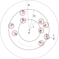
Figure 1. Annulus is covered by small balls

Since $p_{i}\in B(p,2r)\backslash\overline{B(p,r)}$, we may let $p_{i}\in\partial B(p,\beta_{i}r)$ for some $1<\beta_{i}<2$, where $i=1,\ldots,k$. By the first estimate of Proposition 3.1, we have

$$\mathrm{Vol}(B(p,\beta_{i}r)) \leq\mathrm{Vol}(B(p,2r))$$

$$\leq c(n)e^{-\mu}r^{2(n-\delta)}\mathrm{Vol}\left(B(p_{i},\frac{r}{8})\right)$$

for $r\geq c(n)$. By Theorem 2.3, we also have

$$\mathrm{Vol}(B(p,3r))\leq 2\left(1+\frac{6}{\beta_{i}}\right)^{n}\mathrm{Vol}\left(B(p,\beta_{i}r)\right)$$

for $r\geq 2(\sqrt{n}+c)$, where $c:=2\sqrt{n/2}+4n-4/3$ and $i=1,\ldots,k$. Combining the above two estimates, for each $i$,

$$\mathrm{Vol}(B(p,3r))\leq c(n)e^{-\mu}r^{2(n-\delta)}\mathrm{Vol}\left(B(p_{i},\frac{r}{8})\right)$$

for $r\geq c(n)$, where we used $1<\beta_{i}<2$. Summing the above $k$ inequalities, we get

$$k(r)\mathrm{Vol}(B(p,3r))\leq c(n)e^{-\mu}r^{2(n-\delta)}\sum^{k}_{i=1}\mathrm{Vol}\left(B(p_{i},\frac{r}{8})\right)$$

for $r\geq c(n)$. On the other hand, we easily see that

$$\sum^{k}_{i=1}\mathrm{Vol}\left(B(p_{i},\frac{r}{8})\right)\leq\mathrm{Vol}(B(p,3r)).$$

Combining the above two estimates gives

$$k(r)\leq c(n)e^{-\mu}r^{2(n-\delta)}$$

for $r\geq c(n)$, which completes the proof. ∎

Remark 3.3.

In Theorem 3.2, if the scalar curvature also satisfies $\mathrm{S}\leq\sigma$ for some constant $\sigma\geq\delta$ in $M$, then for a sufficiently large $r$, we can choose an $(n-2\delta)$-degree as follows:

$$N=c(n)e^{-\mu}\sigma^{n/2}r^{n-2\delta}.$$

The above weak ball covering property immediately implies Theorem 1.1.

Proof of Theorem 1.1.

Let $(M,g,f)$ be an $n$-dimensional complete non-compact shrinker satisfying (1.1), (1.2) and (1.3). Since the number of ends on the shrinker is independent of the choice of the base point, we can choose a infimum point $p$ of $f$ as a base point in $M$.

Given a sufficiently large fixed number $r$, let

$$N_{1}=c(n)e^{-\mu}r^{2(n-\delta)}$$

as in Theorem 3.2. That is we can find points $p_{1},\ldots,p_{k}\in B(p,2r)\backslash\overline{B(p,r)}$, where $k=k(r)\leq N_{1}$, with

$$\bigcup^{k}_{i=1}B\left(p_{i},\frac{r}{4}\right)\supset B(p,2r)\backslash\overline{B(p,r)}.$$

Next we will prove Theorem 1.1 by a contradiction argument.

If Theorem 1.1 is not true, that is, the number of ends grows faster than polynomial growth with degree $2(n-\delta)$, then for the above mentioned sufficiently large $r$, there exists more than

$$\widetilde{N}_{1}=c(n)e^{-\mu}r^{2(n-\delta)+\epsilon},$$

where $\epsilon>0$ is any small constant, unbounded ends $E_{j}$ with respect to $\overline{B(p,r)}$.

It is obvious that geodesic balls of radius $r/4$ with centers in different components $E_{j}\cap B(p,2r)$ do not intersect. Thus we need at least $\widetilde{N}_{1}$ geodesic balls of radius $r/4$ to cover the sets $E_{j}\cap B(p,2r)\subset B(p,2r)\backslash\overline{B(p,r)}$, which contradicts Theorem 3.2. ∎

Remark 3.4.

For Theorem 1.1, if the scalar curvature $\mathrm{S}\leq\sigma$ for some constant $\sigma\geq\delta$ in $M$, then we can apply Remark 3.3 to the above argument and get the same conclusion whereas the degree $2(n-\delta)$ of polynomial growth can be reduced to $n-2\delta$.

4. Ends with volume comparison condition

In this section we will discuss the finite number of ends when the shrinker satisfies volume comparison condition. In this case we first give a ball covering property, which is similar to the manifold case of nonnegative Ricci curvature.

Theorem 4.1.

Let $(M,g,f)$ be an $n$-dimensional complete non-compact shrinker with a base point $q\in M$ satisfying volume comparison condition. There exists a constant

$$N=N(n,\eta)$$

depending only on $n$ and $\eta$ such that for any $r\geq 2(\sqrt{n}+c)+r_{0}$, where $c:=2\sqrt{f(q)}+4n-4/3$, we can find $p_{1},\ldots,p_{k}\in B(q,2r)\backslash\overline{B(q,r)}$, $k\leq N$, with

$$\bigcup^{k}_{i=1}B\left(p_{i},\frac{r}{4}\right)\supset B(q,2r)\backslash\overline{B(q,r)}.$$

Proof of Theorem 4.1.

Let $k$ be the maximum number of disjoint geodesic balls of radius $r/8$ with centers $p_{1},\ldots,p_{k}$ in $B(q,2r)\backslash\overline{B(q,r)}$. Here we choose $r$ sufficiently large such that $r\geq 2(\sqrt{n}+c)+r_{0}$. Clearly,

$$\bigcup^{k}_{i=1}B\left(p_{i},\frac{r}{4}\right)\supset B(q,2r)\backslash\overline{B(q,r)}.$$

Since $p_{i}\in B(q,2r)\backslash\overline{B(q,r)}$, we may let $p_{i}\in\partial B(q,\beta_{i}r)$ for some constant $1<\beta_{i}<2$, where $i=1,\ldots,k$. By the volume comparison condition, we have

$$\mathrm{Vol}(B(q,\beta_{i}r)) \leq\eta\mathrm{Vol}\left(B(p_{i},\frac{\beta_{i}r}{16})\right)$$

$$\leq\eta\mathrm{Vol}\left(B(p_{i},\frac{r}{8})\right)$$

for all $r\geq r_{0}$. By Theorem 2.3, we see that

$$\mathrm{Vol}(B(q,3r))\leq 2\left(1+\frac{6}{\beta_{i}}\right)^{n}\mathrm{Vol}(B(q,\beta_{i}r))$$

for $r\geq 2\beta_{i}^{-1}(\sqrt{n}+c)$, where $i=1,\ldots,k$. Combining the above two estimates, for each $i$, there exists a constant $C(n,\eta)$ depending only on $n$ and $\eta$ such that

$$\mathrm{Vol}(B(q,3r))\leq C(n,\eta)\mathrm{Vol}\left(B(p_{i},\frac{r}{8})\right)$$

for $r\geq 2(\sqrt{n}+c)+r_{0}$, where $c:=2\sqrt{f(q)}+4n-4/3$ and we used $1<\beta_{i}<2$, where $i=1,\ldots,k$. This implies

$$k\mathrm{Vol}(B(q,3r))\leq C(n,\eta)\sum^{k}_{i=1}\mathrm{Vol}\left(B(p_{i},\frac{r}{8})\right)$$

for $r\geq 2(\sqrt{n}+c)+r_{0}$. On the other hand,

$$\sum^{k}_{i=1}\mathrm{Vol}\left(B(p_{i},\frac{r}{8})\right)\leq\mathrm{Vol}(B(q,3r))$$

Combining the above two inequalities yields $k\leq C(n,\eta)$ and the result follows. ∎

Similar to the preceding discussion in Section 4, we can apply Theorem 4.1 to prove Theorem 1.4. Here we include it for the completeness.

Proof Theorem 1.4.

Under the assumption of Theorem 1.4, we let $N_{2}=N(n,\eta)$ as in Theorem 4.1. If Theorem 1.4 is not true, we can take $r$ large enough such that there exist more than $N_{2}$ unbounded ends $E_{j}$ with respect to $\overline{B(q,r)}$.

Because $E_{j}\cap B(q,2r)$ lie in $B(q,2r)\backslash\overline{B(q,r)}$ and geodesic balls of radius $r/4$ with centers in different components $E_{j}\cap B(q,2r)$ do not intersect. That is, we need more than $N_{2}$ geodesic balls of radius $r/4$ to cover $E_{j}\cap B(q,2r)$, which contradicts Theorem 4.1. ∎

In the rest of this section, we will discuss four sufficient assumptions such that a class of shrinkers satisfies volume comparison condition. As we all know, if $(M,g)$ has nonnegative Ricci curvature everywhere, then it satisfies the volume comparison condition. Indeed the volume doubling property sufficiently leads to volume comparison condition.

Proposition 4.2.

Let $(M,g)$ be an $n$-dimensional complete manifold satisfying the volume doubling property. Then for all $0<r<R<\infty$ and all $x\in M$ and $y\in\overline{B(x,R)}$,

$$\frac{\mathrm{Vol}(B(x,R))}{\mathrm{Vol}(B(y,r))}\leq D^{2}\left(\frac{R}{r}\right)^{\kappa},$$

where $\kappa=\log_{2}D$. In particular, $(M,g)$ satisfies volume comparison condition.

Proof of Proposition 4.2.

Assume $(M,g)$ satisfies the volume doubling property, that is

$$\mathrm{Vol}(B(x,2r))\leq D\,\mathrm{Vol}(B(x,r))$$

for any $x\in M$ and $r>0$, where $D$ is a fixed constant. Let $m$ be a positive integer such that $2^{m}<R/r\leq 2^{m+1}$. Since

$$B(x,R)\subset B(y,2R)\subset B(y,2^{m+2}r)$$

and thus

$$\mathrm{Vol}(B(x,R))\leq\mathrm{Vol}(B(y,2^{m+2}r)),$$

then we have

$$\mathrm{Vol}(B(x,R)) \leq D^{m+2}\mathrm{Vol}(B(y,r))$$

$$\leq D^{2}\left(\frac{R}{r}\right)^{\kappa}\mathrm{Vol}(B(y,r)),$$

where $\kappa=\log_{2}D$. This proves the first estimate.

In particular, when $y\in\partial B(x,R)$, we let $r=R/16$ in the first estimate and immediately get volume comparison condition. ∎

Second, we observe that the shrinker with at least quadratic decay of scalar curvature implies some non-collapsed property and hence satisfies volume comparison condition.

Proposition 4.3.

Let $(M,g,f)$ be a complete non-compact shrinker with a infimum point $p\in M$ of $f$ satisfying (1.1), (1.2) and (1.3). If the scalar curvature satisfies

$$\mathrm{S}(x)\cdot r^{2}(p,x)\leq c_{0}$$

for any $r(p,x)>0$, where $c_{0}>0$ is a constant and $r(p,x)$ is the distance function from $p$ to $x$, then the shrinker satisfies volume comparison condition. In particular, any shrinker with finite asymptotic scalar curvature ratio satisfies volume comparison condition.

Proof of Proposition 4.3.

For any $1/32\leq\alpha\leq 1/2$, for any $r>0$ and for any point $q\in\partial B(p,r)$, by the second estimate of Lemma 2.7, we have

$$(\alpha r)^{-n}\mathrm{Vol}(B(q,\alpha r))\geq c(n)e^{\mu}\left[1+\frac{c_{0}}{(1-\alpha)^{2}r^{2}}\cdot(\alpha r)^{2}\right]^{-\frac{n}{2}}$$

where we used

$$\mathrm{S}\leq\frac{c_{0}}{r^{2}(p,x)}\leq\frac{c_{0}}{(1-\alpha)^{2}r^{2}}.$$

Namely, for any $r>0$ and for any point $q\in\partial B(p,r)$,

$$\mathrm{Vol}(B(q,\alpha r)) \geq c(n)e^{\mu}\left[1+\frac{c_{0}\alpha^{2}}{(1-\alpha)^{2}}\right]^{-\frac{n}{2}}\alpha^{n}\cdot r^{n}$$

$$\geq c(n,c_{0})e^{\mu}r^{n}$$

for some constant $c(n,c_{0})$ depending only on $n$ and $c_{0}$, where used $1/32\leq\alpha\leq 1/2$.

On the other hand, by Lemma 2.5,

$$\mathrm{Vol}(B(p,r))\leq c(n)r^{n}$$

for any $r>0$. Thus, for any $r>0$ and for any point $q\in\partial B(p,r)$, the lower and upper volume estimates give

$$\frac{\mathrm{Vol}(B(p,r))}{\mathrm{Vol}(B(q,\alpha r))}\leq c(n,c_{0})e^{-\mu}.$$

Letting $\alpha=1/16$ shows that such shrinker satisfies volume comparison condition. ∎

The proof of Proposition 4.3 indicates that the finite asymptotic scalar curvature ratio implies the positive asymptotic volume ratio. Moreover, combining Proposition 4.3 and Theorem 1.4, we easily get the following result due to Munteanu, Schulze and Wang [33].

Corollary 4.4.

Any complete non-compact shrinker with finite asymptotic scalar curvature ratio must have finitely many ends.

Third, we see that if a family of the average of scalar curvature integral has at least quadratic decay of radius, then such shrinker also satisfies volume comparison condition.

Proposition 4.5.

Let $(M,g,f)$ be a complete non-compact shrinker with a infimum point $p\in M$ of $f$ satisfying (1.1), (1.2) and (1.3). If there exists a constant $c_{1}>0$ such that

$$\frac{r^{2}}{\mathrm{Vol}\left(B(x,r)\right)}\int_{B(x,r)}\mathrm{S}\,dv\leq c_{1}$$ (4.1)

for all $r>0$ and all $x\in\partial B(p,r)$, then the shrinker satisfies volume comparison condition.

Proof of Proposition 4.5.

For any $r>0$, we let point $q$ be $x\in\partial B(p,r)$ in the first estimate of Lemma 2.7, and get

$$\frac{\mathrm{Vol}\left(B(x,\frac{r}{16})\right)}{(\tfrac{r}{16})^{n}}\left[1+\sup_{s\in\left[0,\tfrac{r}{16}\right]}\frac{s^{2}\int_{B(x,s)}\mathrm{S}\,dv}{\mathrm{Vol}(B(x,s))}\right]^{n/2}\geq c(n)e^{\mu}.$$

By the assumption (4.1), the above inequality becomes

$$\mathrm{Vol}\left(B(x,\frac{r}{16})\right)\geq c(n,c_{1})e^{\mu}r^{n}$$

for all $r>0$ and all $x\in\partial B(p,r)$. Combining this with the volume upper growth $\mathrm{Vol}(B(p,r))\leq c(n)r^{n}$ immediately yields

$$\frac{\mathrm{Vol}(B(p,r))}{\mathrm{Vol}\left(B(x,\frac{r}{16})\right)}\leq c(n,c_{1})e^{-\mu}$$

for any $r>0$ and all $x\in\partial B(p,r)$. ∎

Remark 4.6.

Similar to the above argument, Proposition 4.5 can be also proved by Lemma 2.8. Moreover, when $n\geq 3$, the assumption (4.1) in Proposition 4.5 can be replaced by the bound of the following maximal function of scalar curvature introduced by Topping [39]:

$$\sup_{s\in\left(0,\tfrac{r}{16}\right]}s^{-1}\left[\mathrm{Vol}(B(x,s))\right]^{-\frac{n-3}{2}}\left(\int_{B(x,s)}\mathrm{S}\,dv\right)^{\frac{n-1}{2}}\leq\delta,$$

for all $r>0$ and all $x\in\partial B(p,r)$, where $\delta:=\min\{w_{n},\,(4\pi)^{\frac{n}{2}}e^{\mu+n-2^{n}\cdot 17}\}$ and $\omega_{n}$ is the volume of the unit Euclidean $n$-ball. This bound assumption also enables us to get that

$$\mathrm{Vol}\left(B(x,\frac{r}{16})\right)>\delta\,r^{n}$$

for all $r>0$ and all $x\in\partial B(p,r)$, the interested readers are referred to Theorem 3.1 of [42] for detailed proof.

Combining Proposition 4.5 and Theorem 1.4 leads to

Corollary 4.7.

Any complete non-compact shrinker satisfying (4.1) must have finitely many ends.

In the proof of Corollaries 4.4 and 4.7, we observe that these curvature assumptions both imply a family of Euclidean volume growth. These proof indeed shows that any shrinker with a family of Euclidean volume growth must have volume comparison condition.

Corollary 4.8.

If a complete non-compact shrinker $(M,g,f)$ with a infimum point $p\in M$ of $f$ satisfies

$$\mathrm{Vol}\left(B(x,\frac{r}{16})\right)\geq c\,r^{n}$$ (4.2)

for all $r\geq r_{0}$ for some $r_{0}>0$, and all $x\in\partial B(p,r)$, where $c$ is a positive constant independent of $x$ and $r$, then such shrinker satisfies volume comparison condition and hence has finitely many ends.

In the end of this section, we give some comments on the relation between Corollary 4.8 and asymptotic volume ratio on shrinkers. Recall that the asymptotic volume ratio ($\operatorname{AVR}$) of a complete Riemannian manifold $(M,g)$ is defined by

$$\operatorname{AVR}(g):=\lim_{r\rightarrow\infty}\frac{\operatorname{Vol}B(q,r)}{\omega_{n}r^{n}}$$

if the limit exists. Whenever the $\operatorname{AVR}(g)$ exists, it is independent of point $q$. If $(M,g)$ has nonnegative Ricci curvature, then the limit always exists by the Bishop-Gromov volume comparison. For any shrinker, Chow, Lu and Yang [13] proved that $\operatorname{AVR}(g)$ always exists and is finite. The assumption (4.2) naturally implies positive asymptotic volume ratio; but the reverse problem is not clear to the author at present. Notice that Feldman, Ilmanen and Knopf [17] described examples of complete non-compact Kähler shrinkers, which have $\operatorname{AVR}(g)>0$ and the Ricci curvature changes sign. We see that positive asymptotic volume ratio provides the Euclidean volume growth based on a fixed point, which does not seem to yield a family of Euclidean volume growth (4.2). On the other hand, Carrillo and Ni [7] proved that any shrinker with Ricci curvature $\mathrm{Ric}(g)\geq 0$ must have $\operatorname{AVR}(g)=0$. Here we may reverse the process and naively ask that if $\operatorname{AVR}(g)=0$ implies $\mathrm{Ric}(g)\geq 0$?

5. Diameter growth of ends

In the last section, we will apply the ball covering property to study the diameter growth of ends in the shrinker. The manifold case can be referred to [1], where Abresch and Gromoll proved that every end of manifolds with nonnegative Ricci curvature has most linear diameter growth. Later this result can be generalized by Liu [25] to manifolds with nonnegative Ricci curvature outside a compact set. Let us first recall the definition diameter of ends on manifolds; see also [25].

Definition 5.1.

Let $q$ be a fixed point in a Riemannian manifold $(M,g)$. For any $r>0$, any connected component $\Sigma$ of the annulus

$$A_{q}(2r,\tfrac{3}{4}r):=B(q,2r)\backslash\overline{B(q,\tfrac{3}{4}r)},$$

and any two points $x,y\in\Sigma\cap\partial B(q,r)$, we let

$$d_{r}(x,y):=\inf\left\{\mathrm{length}(\gamma)\right\},$$

where the infimum is taken over all piecewise smooth curves $\gamma$ from $x$ to $y$ in $M\backslash\overline{B(q,r/2)}$. Then we set

$$\mathrm{diam}\left(\Sigma\cap\partial B(q,r)\right):=\sup_{x,y\in\Sigma\cap\partial B(q,r)}d_{r}(x,y).$$

Using the above notations, the diameter of ends at $r$ from $q$ is defined by

$$\mathrm{diam}_{q}(r):=\sup_{\Sigma\subset A_{q}(2r,\tfrac{3}{4}r)}\mathrm{diam}\left(\Sigma\cap\partial B(q,r)\right).$$

See Figure 2 for a simple description.

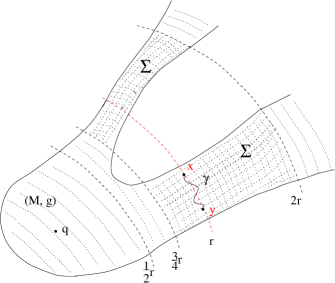
Figure 2. Definition of the diameter of ends

We now apply the above definition to Theorem 5.2 and obtain a diameter growth for ends in the shrinker without any assumption.

Theorem 5.2.

On any $n$-dimensional complete non-compact shrinker with the scalar curvature

$$\mathrm{S}\geq\delta$$

for some constant $\delta\geq 0$, the diameter growth of ends is at most polynomial growth with degree $2(n-\delta)+1$.

Proof of Theorem 5.2.

Without loss of generality, we choose a infimum point $p\in M$ of $f$ as a base point. By Theorem 3.2, for a fixed sufficiently large $r$, and for any connected component $\Sigma$ of the annulus $A_{q}(2r,\tfrac{3}{4}r)$, we can find no more than

$$N:=c(n)e^{-\mu}r^{2(n-\delta)}$$

geodesic balls $B_{i}:=B\left(p_{i},\frac{r}{4}\right)$, where $p_{i}\in A_{q}(2r,\tfrac{3}{4}r)$ and $i\leq N$ such that

$$\bigcup_{i=1}B\left(p_{i},\frac{r}{4}\right)\supset\Sigma.$$

For any two points $x$ and $y$ in $\Sigma\cap\partial B(q,r)$, since $\Sigma$ is connected, we can find a subsequence of geodesic balls $\{B_{i}\}$: $B_{i_{1}},\ldots,B_{i_{k}}$, where $k\leq N$ such that

$$x\in B_{i_{1}},\quad B_{i_{j}}\cap B_{i_{j+1}}\neq\emptyset\,\,(j=1,\ldots,k-1),\quad y\in B_{i_{k}}.$$

Now we choose fixed points $z_{j}\in B_{i_{j}}\cap B_{i_{j+1}}$ and consecutively connect the above mentioned points

$$x,p_{i_{1}},z_{1},p_{i_{2}},z_{2},p_{i_{3}},\ldots,p_{i_{k-1}},z_{k-1},p_{i_{k}},y,$$

which forms a piecewise smooth curve $\gamma$. Obviously, the curve $\gamma$ lies in $M\backslash\overline{B(q,r/2)}$ and has the length of $\gamma$

$$\mathrm{length}(\gamma)\leq 2k\cdot\frac{r}{4}\leq\frac{N}{2}r\leq c(n)e^{-\mu}r^{2(n-\delta)+1}.$$

This completes the proof. ∎

Remark 5.3.

If the scalar curvature of shrinker is uniformly bounded, by Remark 3.3, the above argument indicates that the degree $2(n-\delta)+1$ in Theorem 5.2 can be reduced to $n-2\delta+1$.

If the shrinker satisfies volume comparison condition, by the same argument as above, Theorem 4.1 immediately implies

Theorem 5.4.

On any complete non-compact shrinker with volume comparison condition, the diameter growth of ends is at most linear.

References

- [1] U. Abresch, D. Gromoll, On complete manifolds with nonnegative Ricci curvature, J. Amer. Math Soc. 3 (1990), 355-374.
- [2] D. Bakry, M. Emery, Diffusion hypercontractivitives, in: Séminaire de Probabilités XIX, 1983/1984, in: Lecture Notes in Math., vol. 1123, Springer-Verlag, Berlin, 1985, pp. 177-206.
- [3] M.-L. Cai, Ends of Riemannian manifolds with nonnegative Ricci curvature outside a compact set, Bulletin of the AMS, 24 (1991), 371-377.
- [4] H.-D. Cao, Recent progress on Ricci solitons, Recent advances in geometric analysis, Adv. Lect. Math. (ALM) 11, 1-38, International Press, Somerville, MA 2010.
- [5] H.-D. Cao, Geometry of complete gradient shrinking Ricci solitons, in Geometry and Analysis I, Adv. Lect. Math. 17 (2011), 227-246.
- [6] H.-D. Cao, D. Zhou, On complete gradient shrinking Ricci solitons, J. Diff. Geom. 85 (2010), 175-186.
- [7] J. Carrillo, L. Ni, Sharp logarithmic Sobolev inequalities on gradient solitons and applications, Commun. Anal. Geom. 17 (2009), 721-753.
- [8] J. Cheeger, D. Gromoll, The splitting theorem for manifolds of nonnegative Ricci curvature. J. Diff. Geom. 6 (1971/72), 119-128.
- [9] J. Cheeger, G. Tian, Curvature and injectivity radius estimates for Einstein 4-manifolds, J. Amer. Math. Soc. 19 (2005) 487-525.
- [10] B.-L. Chen, Strong uniqueness of the Ricci flow, J. Diff. Geom. 82 (2009), 363-382.
- [11] B. Chow, S.C. Chu, D. Glickenstein, C. Guenther, J. Isenberg, T. Ivey, D. Knopf, P. Lu, F. Luo, L. Ni, The Ricci flow: techniques and applications, part IV: long-time solutions and related topics, Mathematical surveys and Monographs, vol. 206, American Mathematical Society.
- [12] B. Chow, P. Lu, B. Yang, Lower bounds for the scalar curvatures of noncompact gradient Ricci solitons, Comptes Rendus Mathematique, 349 (2011), 1265-1267.
- [13] B. Chow, P. Lu, B. Yang, A necessary and sufficient condition for Ricci shrinkers to have positive AVR, Proc. Amer. Math. Soc. 140 (2012), 2179-2181.
- [14] A. Derdziński, A Myers-type theorem and compact Ricci solitons, Proc. Amer. Math. Soc. 134 (2006), 3645-3648.
- [15] J. Enders, R. Müller, P. Topping, On Type-I singularities in Ricci flow, Comm. Anal. Geom. 19 (2011), 905-922.
- [16] F.-Q. Fang, J.-W. Man, Z.-L. Zhang, Complete gradient shrinking Ricci solitons have finite topological type, C. R. Math. Acad. Sci. Paris 346 (2008), 653-656.
- [17] M. Feldman, T. Ilmanen, D. Knopf, Rotationally symmetric shrinking and expanding gradient Kähler-Ricci solitons. J. Diff. Geom. 65 (2003), 169-209.
- [18] H.-B. Ge, S.-J. Zhang, Liouville-type theorems on the complete gradient shrinking Ricci solitons, Diff. Geome. App. 56 (2016), 42-53.
- [19] R. Hamilton, The Formation of Singularities in the Ricci Flow. Surveys in Differential Geometry, International Press, Boston, vol. 2, (1995), 7-136.
- [20] R. Haslhofer, R. Müller, A compactness theorem for complete Ricci shrinkers, Geom. Funct. Anal. 21 (2011), 1091-1116.
- [21] R. Haslhofer, R. Müller, A note on the compactness theorem for 4d Ricci shrinkers, Proc. Amer. Math. Soc. 143 (2015), 4433-4437.
- [22] S.-S. Huang, -regularity and structure of four-dimensional shrinking Ricci solitons, Int. Math. Res. Not. IMRN 2020, no. 5, 1511-1574.
- [23] S.-S. Huang, Y. Li, B. Wang, On the regular-convexity of Ricci shrinker limit spaces, Crelle’s Journal, 2021, (2021), no. 771, 99-136
- [24] B. Kotschwar, L. Wang, Rigidity of asymptotically conical shrinking gradient Ricci solitons, J. Diff. Geom. 100 (2015), 55-108.
- [25] Z.-D. Liu, Ball covering property and nonnegative Ricci curvature outside a compact set. Proc. Symp. Pure Math. 54, (1993), 459-464.
- [26] H.-Z. Li, Y. Li, B. Wang, On the structure of Ricci shrinkers, J. Funct. Anal. 280 (2021), no. 9, Paper No. 108955, 75 pp.
- [27] P. Li, Geometric Analysis, Cambridge Studies in Advanced Mathematics, vol. 134 (2012), Cambridge University Press, New York.
- [28] P. Li, L.-F. Tam, Harmonic functions and the structure of complete manifolds, J. Diff. Geom. 35 (1992), 359-383.
- [29] P. Li, L.-F. Tam, Green’s function, harmonic functions and volume comparison, J. Diff. Geom. 41 (1995) 277-318.
- [30] Y. Li, Ricci flow on asymptotically Euclidean manifolds. Geom. Topol. 22 (2018), 1837-1891.
- [31] Y. Li, B. Wang, The rigidity of Ricci shrinkers of dimension four, Trans. Amer. Math. Soc. 371 (2019), 6949-6972.
- [32] Y. Li, B. Wang, Heat kernel on Ricci shrinkers, Calc. Var. PDEs, 59 (2020) Art. 194.
- [33] O. Munteanu, F. Schulze, J.-P. Wang, Positive solutions to Schrödinger equations and geometric applications, J. Reine Angew. Math. 774 (2021), 185-217.
- [34] O. Munteanu, J.-P. Wang, Analysis of weighted Laplacian and applications to Ricci solitons. Commun. Anal. Geom. 20 (2012), 55-94.
- [35] O. Munteanu, J.-P. Wang, Geometry of manifolds with densities, Adv. Math. 259 (2014), 269-305.
- [36] O. Munteanu, J.-P. Wang, Holomorphic functions on Kähler-Ricci solitons, J. Lond. Math. Soc. 89 (2014), 817-831.
- [37] G. Perelman, The entropy formula for the Ricci flow and its geometric applications, arXiv:math.DG/0211159.
- [38] S. Pigola, M. Rimoldi, A.G. Setti, Remarks on non-compact gradient Ricci solitons, Math. Z. 268 (2011), 777-790.
- [39] P. Topping, Diameter control under Ricci flow, Comm. Anal. Geom. 13 (2005), 1039-1055.
- [40] J.-Y. Wu, Elliptic gradient estimates for a weighted heat equation and applications, Math. Z. 280 (2015), 451-468.
- [41] J.-Y. Wu, Counting ends on complete smooth metric measure spaces, Proc. Amer. Math. Soc. 144 (2016), 2231-2239.
- [42] J.-Y. Wu, Sharp upper diameter bounds for compact shrinking Ricci solitons. Ann. Global Anal. Geom. 60 (2021), 19-32.
- [43] J.-Y. Wu, Geometric inequalities and rigidity of gradient shrinking Ricci solitons, arXiv:2009.12725.
- [44] J.-Y. Wu, P. Wu, Heat kernel on smooth metric measure spaces with nonnegative curvature, Math. Ann. 362 (2015), 717-742.
- [45] J.-Y. Wu, P. Wu, Heat kernel on smooth metric measure spaces and applications, Math. Ann. 365 (2016), 309-344.
- [46] W. Wylie, Complete shrinking Ricci solitons have finite fundamental group, Proc. Amer. Math. Soc. 136 (2008), 1803-1806.
- [47] S.-J. Zhang, On a sharp volume estimate for gradient Ricci solitons with scalar curvature bounded below, Acta Mathematica Sinica, English Series 27 (2011), 871-882.