Rodlike Heisenberg nanomagnet driven by propagating magnetic field: Nonequilibrium phase transition

Muktish Acharyya^∗

Department of Physics, Presidency University,
86/1 College Street, Kolkata-700073, India

Email^∗:muktish.physics@presiuniv.ac.in

Abstract: The dynamical responses of a rodlike anisotropic Heisenberg ferromagnet, irradiated by the propagating magnetic field wave, have been studied by Monte Carlo simulation using Metropolis single spin-flip algorithm. A nonequilibrium dynamical phase transition has been observed. The transition temperature has been obtained from the peak position of the variance of the dynamic order parameter plotted as a function of the temperature. The transition has been found to occur at a lower temperature for the higher value of the amplitude of the propagating magnetic field wave. A comprehensive phase boundary was drawn. The phase boundary has been found to be insensitive to the wavelength of the propagating field wave. The boundary encloses more area of the region of the ordered phase for stronger anisotropy.

Keywords: Heisenberg ferromagnet, Monte Carlo simulation, Metropolis algorithm, Magnetic anisotropy

I. Introduction

The studies on magnets have taken important places in modern research over several decades due to various interesting physical phenomena and commercial applications. The study of the magnetic materials in the nanometer scale has drawn additional attention to the modern research[1, 2]. The most important applications of such nanomagnetic devices, in the field of magnetic storage, are mainly due to the advanced technological features[3]. The basic challenge is to develop a nanomagnetic device with a very high density of storage.

The theoretical research, to study the behaviors of tiny magnetic materials, is also advancing in parallel to the experimental research. The dynamics of Ising like core-shell nanoparticle [4, 5] and the dynamical responses of uniaxial nanomagnetic system driven by an oscillating magnetic field are recently studied [6]. The simple Ising type interaction was considered to have the response of such kinds of systems on a small length scale. The uniaxial nanowire has been investigated[7] to study the nonequilibrium phase transition.

The rodlike nanomagnets have also been investigated recently. The cylindrical magnetic nanowire driven by propagating magnetic field wave has been investigated[8] recently with extensive Monte Carlo simulation to get interesting nonequilibrium phase transition. The results of magneto-kinetic properties have been reported[9] in cylindrical Ising nanotube. The dynamic responses of hexagonal Ising nanowire have been investigated[10]. The cylindrical Ising nanowire, driven by an oscillating magnetic field, has shown[11] a nonequilibrium phase transition.

All the simulational studies mentioned above are mainly based on the Ising type interaction among the magnetic spins. This Ising type interaction could be the best model of highly anisotropic magnetic systems. The phase boundary of the nonequilibrium phase transition can depend on the anisotropy of the magnetic system. Such kind of variation cannot be observed in the case of Ising-like interaction. In this context, the most general classical spin model is the anisotropic Heisenberg model. In this paper, the classical anisotropic Heisenberg model is used to study the dynamical responses of a rodlike nanomagnet irradiated by propagating magnetic field waves. This will serve as the general model to study the response of rodlike nanomagnet to the optical perturbations.

The manuscript is organized as follows: the next section (section-II) is devoted to introducing the model, section-III describes the simulational scheme, the numerical results are reported in section-IV, the paper ends with a summary in section-V.

II. The Model of rodlike Heisenberg nanoferromagnet:

Here, the system of interest is the anisotropic classical Heisenberg ferromagnet. It can be represented by the following Hamiltonian

$$H=-J\sum_{<ij>}{\vec{S}_{i}}\cdot{\vec{S}_{j}}-D\sum_{i}(S_{i}^{z})^{2}-\sum{\vec{H}(i,j,t)}\cdot{\vec{S}_{i}}$$ (1)

where the ${\vec{S}_{i}}$ represents the Heisenberg spin vector ($|{\vec{S}_{i}}|=1$) at i-th site, having three cartesian components $(S_{i}^{x},S_{i}^{y},S_{i}^{z})$. The first term in the above expression represents the contribution to the energy arises due to spin-spin Heisenberg nearest neighbour ($<ij>$) ferromagnetic ($J>0$) interaction. The second term is the single-site anisotropy (crystal field with z-axis as easy axis) and the third is the Zeeman term where the interaction of spin with externally applied space-time dependent magnetic field ${\vec{H}(i,j,t)}$ (measured in the unit of $J$). The space-time dependent magnetic field is propagating along the z-direction (represented by the index k of the three-dimensional lattice) and is polarized in the x-direction with the following mathematical form:

$$H(i,j,t)=h_{x}{\rm cos}[2\pi(ft-k/{\lambda})]$$ (2)

where $h_{x}$ is the amplitude, $f$ is the frequency and $\lambda$ is the wavelength of the propagating magnetic field wave.

Here, the propagating magnetic field is considered as the magnetic component of the propagating electromagnetic wave, keeping in mind, to study the response of Heisenberg nanomagnetic rod irradiated by an electromagnetic field. Here, the magnetic polarisation of the transverse EM wave (propagating in the z-direction) is considered in the x-direction.

The geometry of the system is quasi one dimensional of size $N=L_{x}\times L_{y}\times L_{z}$ where $L_{x}=L_{y}=4$ and $L_{z}=200$. This describes the structure of rodlike Heisenberg nanomagnet. The magnetic wave is propagating in the z-direction. The system is exposed to the open boundary conditions in all directions.

III. Monte Carlo methods applied to Heisenberg nanomagnet:

The system is initially kept at a very high temperature, guaranteed by the random spin configuration of the paramagnetic phase. Then the magnetic field is applied. The magnetic field (space-time dependent) is propagating along the z-direction (longitudinal axis of the system considered here). The space-time-dependent magnetic field keeps the system far away from the equilibrium. However, the nonequilibrium steady state of the system can be achieved at any lower temperature by cooling the system slowly from the initial high-temperature spin configuration.

The spins of the system are updated by a random updating scheme with Metropolis single spin-flip algorithm. A lattice site is chosen randomly. The initial spin state of that site is noted. A trial spin configuration of that chosen site is chosen randomly. The change in energy ($\Delta H$) has been calculated from the given form of the Hamiltonian (equation-1) with nearest-neighbor interactions. This trial spin configuration will be accepted with Metropolis probability[12, 13]

$$P({\vec{S}}_{i}^{initial}\to{\vec{S}}_{i}^{final})={\rm Min}[1,e^{({{-\Delta H}\over{kT}})}]$$ (3)

The trial spin configuration will be accepted if another random number (uniformly distributed between 0 and 1) is less than or equal to the Metropolis probability mentioned above (equation-2). In this way, $N$ number of such updates have been done. $N$ such random updates constitute the time unit and are termed as MCSS (Monte Carlo Step per Site). At any fixed temperature, $16\times 10^{5}$ MCSS are allowed. The initial $8\times 10^{5}$ MCSS are discarded (as assumed the transient period to achieve the nonequilibrium steady state (NESS)). The quantities are measured from the averaging over the next $8\times 10^{5}$ MCSS. The stepsize of the temperature for cooling the system was considered $\Delta T=0.05$. The unit of temperature is $J/k$. This value of $\Delta T$ is assumed to be small enough to move from one nonequilibrium steady state (NESS) to lower temperature NESS.

IV. Simulational results:

We are mainly interested to study the nonequilibrium phases depending on the temperature of the system. In this context, the relevant measurable quantities would be the component of the nonequilibrium dynamic order parameter, the variance of that component of the order parameter (so-called susceptibility). Keeping these in mind, the following quantities are calculated:

(i) Components of instantaneous magnetisation $m_{\alpha}(t)={{1}\over{N}}\sum S_{i}^{\alpha}$ where $\alpha$ denotes different Cartesian components, $\alpha=x,y,z$.

(ii) Components of time averaged magnetisation over a full cycle of the propagating magnetic field: $q_{\alpha}={{1}\over{f}}\int m_{\alpha}(t)dt$. and $Q_{\alpha}=<q_{\alpha}>$. The averaging, represented by $<...>$, has been calculated over various cycles of the propagating magnetic field. In this study, the frequency of the propagating magnetic wave is considered $f=0.01$. So the 100 MCSS will constitute a complete cycle of the wave. This quantity $Q_{\alpha}$ serves as the dynamical order parameter. It may be mentioned here that such a vector order parameter was introduced [14, 15] in the Monte Carlo study of Heisenberg ferromagnets and verified experimentally [16, 17, 18, 19] afterwards.

(iii) The variance of the dynamic order parameter:

$\chi_{\alpha}=N(<q^{2}_{\alpha}>-<q_{\alpha}>^{2})$

The z-component of the dynamical order parameter has been investigated as a function of temperature (T) to study the nonequilibrium phase transition. The dynamical order parameter, $Q_{z}$, was observed to become nonzero at any finite temperature ($T_{d}$) if the system was cooled down from a high temperature ($Q_{z}=0$) for a fixed set of $\lambda$, $D$, and $h_{x}$ values. This indicates the nonequilibrium phase transition. The direction of polarisation of the magnetic field (of the propagating wave) and the easy anisotropy axis would make $Q_{x}=Q_{y}=0$. Here, the dynamic ordering is possible only in the z-direction.

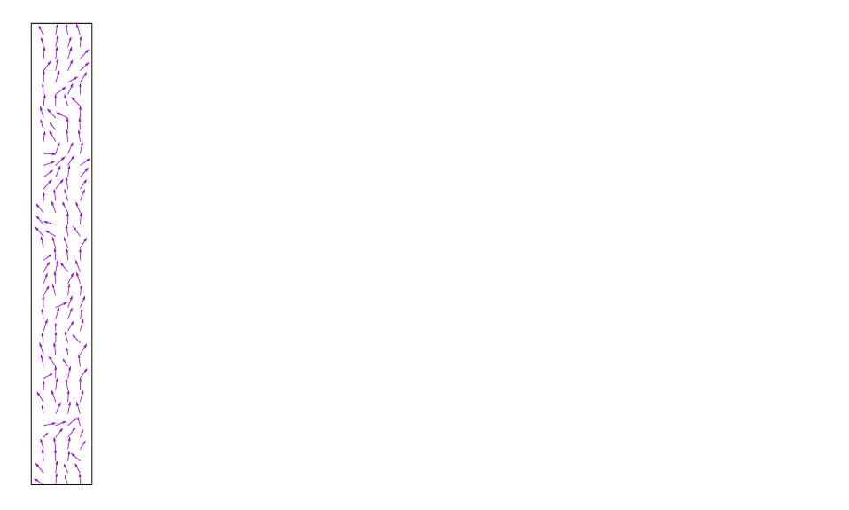
(a)

(b)

Figure 1: Longitudinal cross sections of Spin projections at $t=16000$ MCSS (a) $T=0.60$ and (b) $T=2.40$. Here, $D=0.50$, $h_{x}=1.20$, $f=0.01$ and $\lambda=10$. The direction of propagation is upward.

The longitudinal cross-section of the spin projections is shown in Fig. -1 for two different values of temperature at any instant of time, t = 16000 MCSS. The ordered structure is shown in the low temperature ($T=0.60$) configuration (Fig-1(a)), which provides the dynamically ordered phase.However, this ordered structure disappears at high temperatures ($T=2.40$) in a dynamically disordered phase (Fig. 1(b)).

The transition temperature, for this nonequilibrium dynamical phase transition, is denoted as $T_{d}$. The transition occurs at a lower temperature for a higher value of applied field amplitude $h_{x}$. One such typical plot is shown in Fig-2(a). Here, we have used, $D=0.5$, $\lambda=10$. The frequency $f$ of the propagating magnetic field was kept fixed ($f=0.01$) throughout the study. The dynamical ordering takes place at higher temperature for $h_{x}=0.4$.

The variance ($\chi_{z}$) of the dynamic order parameter ($Q_{z}$) was studied as a function of the temperature and is plotted in Fig-2(b). The variance was found to be peaked sharply (assumed to have diverged in thermodynamic limit) at the dynamic transition temperature $T_{d}$. For, $h_{x}=0.4$ the transition occurs at $T_{d}=1.2$ and for $h_{x}=1.2$ the transition occurs at $T=0.95$. In fact, to measure $T_{d}$, the position of the peak of the variance of the dynamic order parameter was used here. The variations, of the order parameter $Q_{z}$) and its variance $\chi$ near the transition temperature, are consistent with those observed generally in the case of equilibrium phase transitions. It may be noted here (as observed also) that the transition temperature $T_{d}$ depends on the amplitude ($h_{x}$) of the propagating magnetic field wave. It is found that the dynamic transition occurs at lower temperatures for higher values of $h_{x}$.

Do we expect any significant dependence of the transition temperature on the wavelength ($\lambda$) of the propagating field wave? To know the answer, we have studied this for a different value of $\lambda$ and shown the results in Fig-2(c) (the temperature dependences of the order parameter) and Fig-2 (d) (the temperature dependences of the variance of the dynamic order parameter). No such significant changes in the dynamic transition temperature were observed in this case. That will be clearly shown in the phase diagram.

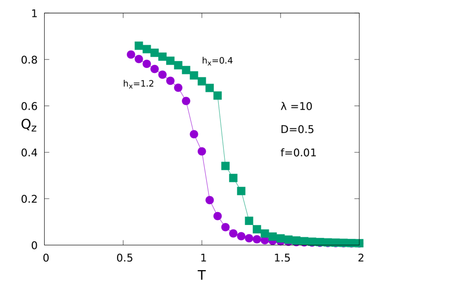
(a)

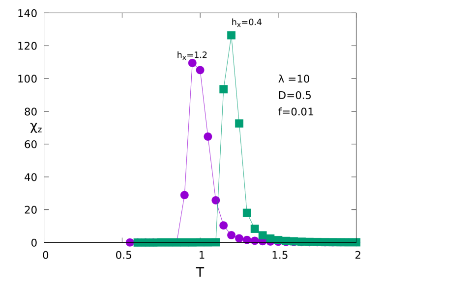
(b)

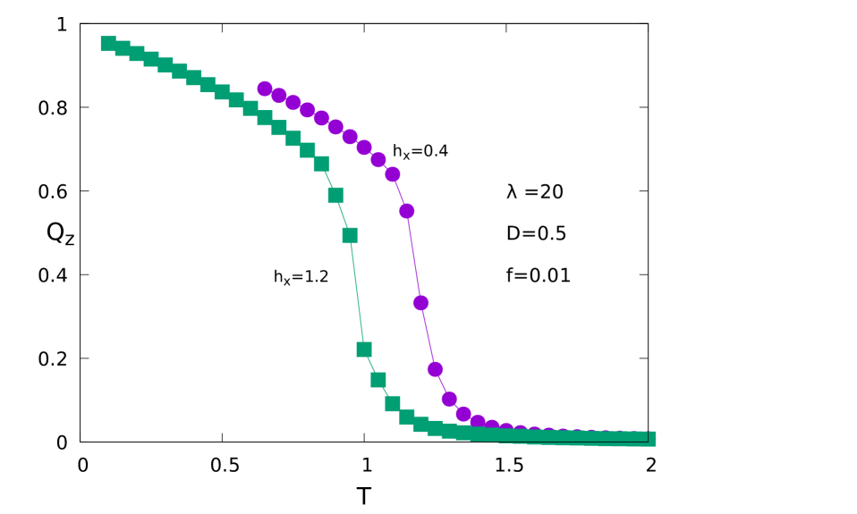
(c)

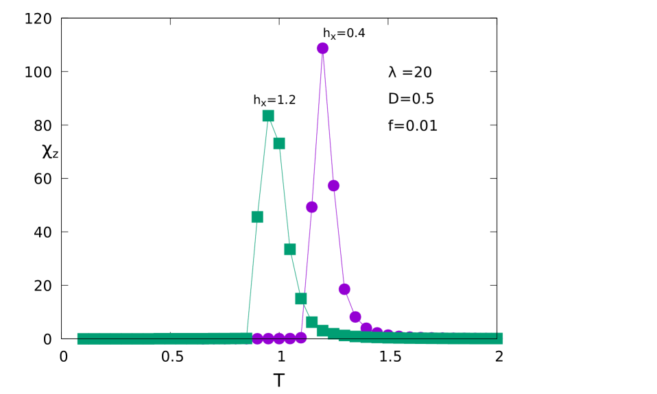
(d)

Figure 2: The order parameters ($Q_{z}$) and its variances ($\chi_{z}$) are plotted against the temperature ($T$) for $D=0.5$. Here, $L_{z}=200$.

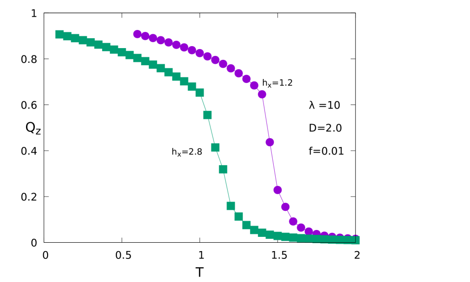
(a)

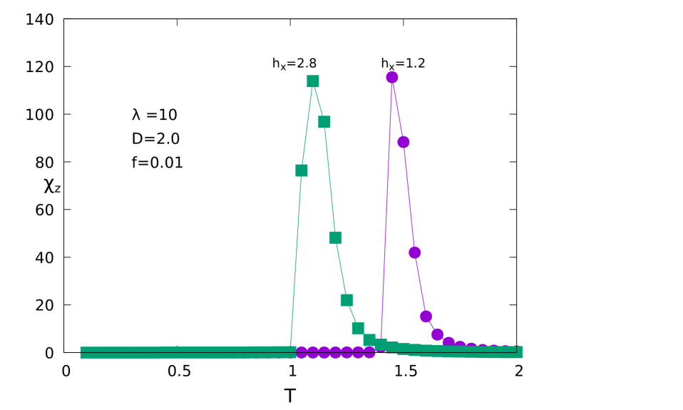
(b)

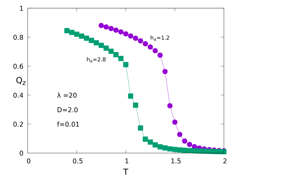
(c)

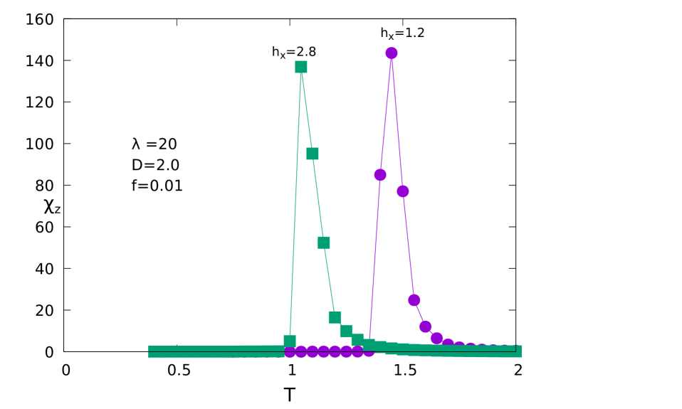
(d)

Figure 3: The order parameters ($Q_{z}$) and its variances ($\chi_{z}$) are plotted against the temperature ($T$) for $D=2.0$. Here, $L_{z}=200$.

However, we have observed significant changes in the dynamic transition temperature ($T_{d}$) as the strength of anisotropy is changed. The same studies mentioned above (and the results shown in Fig-2) are done for a different value of the strength of anisotropy, $D=2.0$. For other parameters held constant ($h_{x}=1.2$, $\lambda=10$, and $f=0.01$), the transition temperature was found to increase (as shown in Fig-3(a) and Fig-3(b)). In this case, the transition temperature was found at $T_{d}=1.45$ (it was $T_{d}=0.95$ for $h_{x}=1.2$, $D=0.5$, and $\lambda=10$ as shown in Fig.2(b)). The transition temperature did not change significantly when the wavelength of the propagating magnetic field wave ($\lambda=20$) was increased. These are shown in Fig. 3(c) and Fig. 3(d).

A comprehensive phase boundary has been drawn on the $T_{d}-h_{x}$ plane with $lambda$ and $D$ being different parameters. The peak position of the variance ($\chi_{z}$) of the dynamic order parameter was used to estimate the dynamic transition temperatures $T_{d}$ for different parameters. Fig-4(a) shows such a phase diagram for $D=0.5$, $f=0.01$ and two different values of $\lambda$. The region of non-zero (dynamically ordered phase) $Q_{z}$ and the region of $Q_{z}=0$ (dynamically disordered phase) are shown. The phase diagrams of two different values of $\lambda$ (=10 and 20) are shown in different symbols (and with different colors). The phase boundaries do not show any significant dependence on the wavelengths of the propagating magnetic field waves. The same kinds of phase diagrams are shown (in Fig-4(b)) for different values of the strength of anisotropy $D=2.0$. Here the significant variation of the phase boundary is observed. For the higher value of the anisotropy, the region of the ordered phase (non-zero $Q_{z}$) is expanded.

The variance ($\chi_{z}$) of the dynamic order parameter ($Q_{z}$) has been studied as a function of temperature ($T$) for different values of $L_{z}$. The results are shown in Fig-5. The height of the peak of $\chi_{z}$ has been observed to increase as the length ($L_{z}$) of the nanorod increases. This is a sign of the growth of dynamic correlations near the transition temperature. This will eventually diverge for $L_{z}\to\infty$ indicating the true phase transition (of nonequilibrium kind) in the thermodynamic limit.

The peak values ($\chi_{z}^{m}$) of the variances ($\chi_{z}$) of the order parameter ($Q_{z}$) for different longitudinal sizes ($L_{z}$=40,60,80,120 and 160 here) of the system are plotted in logarithmic scale and shown in Fig-6. The data points are fitted in a power law $\chi^{p}_{z}\sim(L_{z})^{{\gamma}\over{\nu}}$. Here the estimation of the exponent ${{\gamma}\over{\nu}}=1.1887\pm 0.1645$. The goodness of fit has been analyzed by the standard $\chi^{2}$ test. The value of the $\chi^{2}$ for three degrees of freedom (here we have five data points and two fitting parameters) is 2.206 which is much less than the value (7.810) of that of five percent significant level.

We have also studied the size ($L_{z}$) dependence of the dynamic transition temperature ($T_{d}$) and shown in Fig-7. Here, the dynamic transition temperatures for different lengths ($L_{z}$) of the nanorod are studied. The plot of $T_{d}$ against the $L_{z}$ does not show any remarkable dependence of the transition temperature ($T_{d}$) on the length of the nanorod $L_{z}$.

V. Summary

The tiny anisotropic Heisenberg ferromagnet (rodlike) in the presence of propagating magnetic field wave has been studied by Monte Carlo simulation using Metropolis single spin-flip algorithm. The direction of propagation of the magnetic wave has been considered here as the z-direction (which is an easy anisotropy axis here). The z-component of the time-averaged magnetization over a complete cycle of the propagating field was found to assume nonzero value at any finite temperature if the system is cooled down from high temperature. This acts as the order parameter of such a nonequilibrium phase transition. This is an indication of the nonequilibrium phase transition. The transition temperature was found from the temperature dependence of the variance of the component of the dynamic order parameter. The dynamic transition was found to occur at a lower temperature for the higher value of the amplitude of the propagating magnetic field wave. A comprehensive phase boundary was drawn. The phase boundary does not show any significant deviation if the wavelength of the propagating wave changes. But notable changes of the phase boundary were observed as the strength of anisotropy changes. The region of the ordered phase was found to expand for a stronger value of anisotropy.

The size dependence of the variance of the component of the dynamic order parameter shows the growth of dynamic correlation in the vicinity of the dynamic transition temperature. The size dependence of the transition temperature ($T_{d}$) does not show any significant changes within the domain of length of the nanorod considered in this study.

One may think of reducing the size of the cross-sectional area of the nanorod to make the system quasi-one-dimensional. A question may arise whether the nonequilibrium phase transition can be observed in such a quasi-one-dimensional system. However, we have to keep in mind the following two important issues in this context. (i) As pointed out by the Mermin-Wagner theorem that classical Heisenberg ferromagnet can show long-range ferromagnetic ordering (Ferro-para phase transition) only above two dimensions and this is an equilibrium concept. (ii) Here the transition studied is a nonequilibrium type which is an outcome of the competition between the intrinsic timescale (relaxation time) of the system and the tunable (time period) timescale of the external field. It may be mentioned here that this kind of dynamic phase transition disappears [20] in the vanishingly small frequency limit, in all dimensions, not only in one dimension.

V. Acknowledgements

The financial support through FRPDF, Presidency University is gratefully acknowledged.

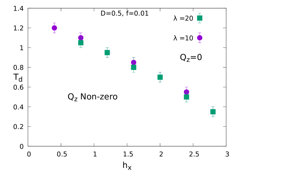
(a)

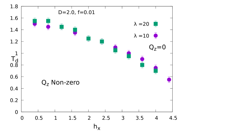
(b)

Figure 4: The phase diagrams of nonequilibrium phase transitions. (a) for D=0.5 and (b) for D=2.0. Here $L_{z}=200.$

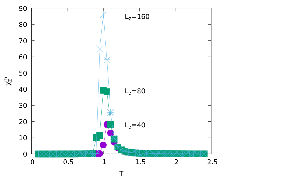
Figure 5: The variances ($\chi_{z}$) of the order parameter ($Q_{z}$) are plotted against the temperature ($T$) for different longitudinal sizes ($L_{z}$) of the nanorod.Here, $D=0.5,\lambda=10,h_{x}=1.2$ and $f=0.01$.

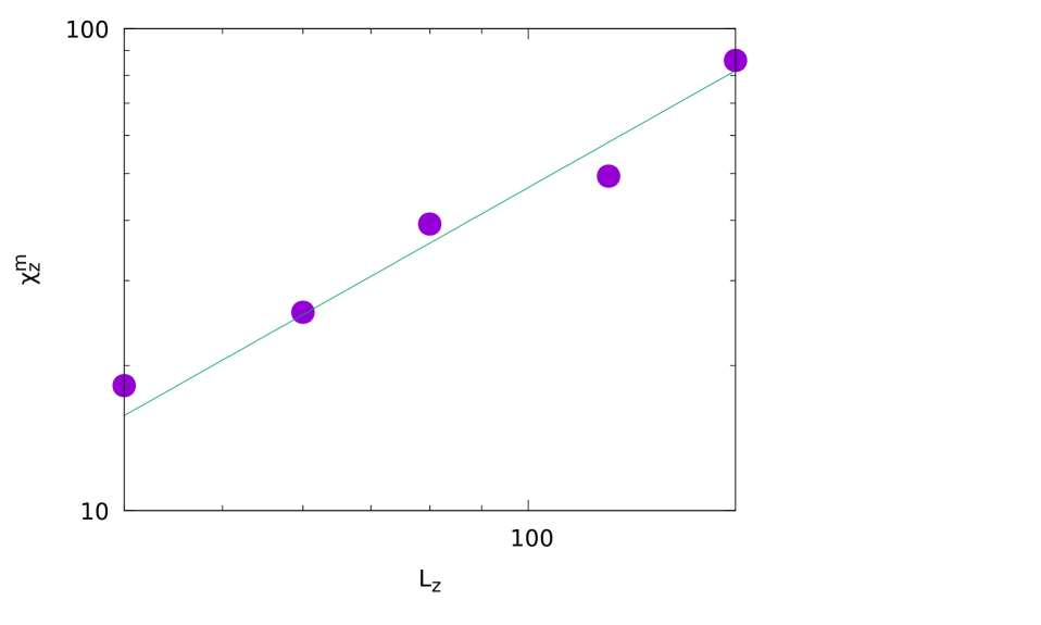
Figure 6: The maxima ($\chi^{m}_{z}$) of the variances ($\chi_{z}$) of the order parameter ($Q_{z}$) have been plotted against the longitudinal sizes ($L_{z}$) of the nanorod , in logarithmic scale. The solid line represent the fitting function $Y=0.196X^{1.1887}$. Here, $D=0.5,\lambda=10,h_{x}=1.2$ and $f=0.01$.

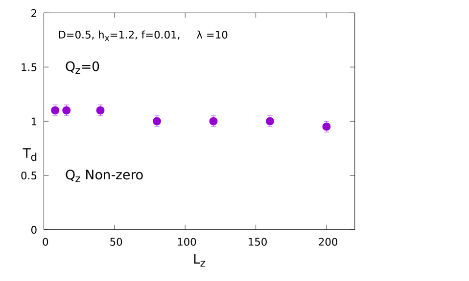
Figure 7: The nonequilibrium phase transition temperature $T_{d}$ is plotted against the different longitudinal sizes ($L_{z}$) of the nanorod.

References

- [1] Bivas Rana, Amrit Kumar Mondal, Supriyo Bandyopadhyay and Anjan Barman, arxiv:2102.12436.
- [2] M.I. Irshad, F. Ahmad and N.M. Mohamed, AIP Conf. Proc., vol. 1482, (2012) 625.
- [3] S. Bedanta, A. Barman, W. Kleemann, O. Petracic, and T. Seki, Journal of Nanomaterials, 2013 (2013) 952540
- [4] E. Vatansever and M. Acharyya, J. Magn. Magn. Mater., 527 (2021) 167721
- [5] E. Kantar, B. Deviren and M. Keskin, Eur. Phys. J. B., 86, (2013) 253.
- [6] Y. Yuksel, Phys. Rev. E, 91 (2015) 032149
- [7] Y. Yüksel, J. Magn. Magn. Mater., 389, (2015) 34.
- [8] E. Vatansever, Academic Platform Journal of Engineering and Science 6, (2018) 72
- [9] B. Deviren, Y. Sener, M. Keskin, 392, (2013) 3983.
- [10] M. Ertaş and Y. Kocakaplan, Phys. Lett. A, vol. 378, (2014) 845.
- [11] B. Deviren, E. Kantar and M. Keskin, J. Magn. Magn. Mater., 324, (2012) 2163.
- [12] K. Binder, Monte Carlo Methods in Statistical Physics, Springer, Berlin, 1979.
- [13] M.E.J. Newman and G.T. Barkema, Monte Carlo Methods in Statistical Physics, Clarendon Press, Oxford, 2001.
- [14] M. Acharyya, Phys. Rev. E, 69 (2004) 027105
- [15] M. Acharyya, Int. J. Mod. Phys. C, 17 (2006) 1107
- [16] D.T. Robb, Y.H. Xu, O. Hellwig, J. McCord, A. Berger, M.A. Novotny and P.A. Rikvold, Phys. Rev. B., 78, (2008) 134422.
- [17] M. Quintana and A. Berger, Phys. Rev. E, 104 (2021) 044125
- [18] A. Berger, O. Idigoras and P. Vavassori, Phys. Rev. Lett., 111, (2013) 190602.
- [19] P. Riego, P. Vavassori and A. Berger, Phys. Rev. Lett., 118, (2017) 117202.
- [20] B. K. Chakrabarti and M. Acharyya, Rev. Mod. Phys. 71 (1999) 847