Extended phase-space symplectic-like integrators for coherent post-Newtonian Euler-Lagrange equations

Abstract

Coherent or exact equations of motion for a post-Newtonian Lagrangian formalism are the Euler-Lagrange equations without any terms truncated. They naturally conserve energy and angular momentum. Doubling the phase-space variables of positions and momenta in the coherent equations, we establish extended phase-space symplectic-like integrators with the midpoint permutations. The velocities should be solved iteratively from the algebraic equations of the momenta defined by the Lagrangian during the course of numerical integrations. It is shown numerically that a fourth-order extended phase-space symplectic-like method exhibits good long-term stable error behavior in energy and angular momentum, as a fourth-order implicit symplectic method with a symmetric composition of three second-order implicit midpoint rules or a fourth-order Gauss-Runge-Kutta implicit symplectic scheme does. For given time step and integration time, the former method is superior to the latter integrators in computational efficiency. The extended phase-space method is used to study the effects of the parameters and initial conditions on the orbital dynamics of the coherent Euler-Lagrange equations for a post-Newtonian circular restricted three-body problem. It is also applied to trace the effects of the initial spin angles, initial separation and initial orbital eccentricity on the dynamics of the coherent post-Newtonian Euler-Lagrange equations of spinning compact binaries.

I Introduction

Gravitational waves and black holes are two fundamental predictions of the theory of Einstein’s general relativity. The predictions were recently confirmed by a series of detections of gravitational waves, such as GW150914 1 and GW190521 [2, 3]. Chaos is a possibly terrible obstacle to a method of matched filtering, which requires a gravitational wave signal drawn out of the noise in excellent agreement with a theoretical template of the gravitational wave [4]. Thus, chaos in systems of spinning compact binaries has been studied by several authors [4-14]. The chaotic behavior in these references was mainly considered in conservative binary systems. In fact, chaos may be irrelevant in dissipative binary black hole systems due to the fast dissipation [15].

Higher-order post-Newtonian (PN) approximations are well applicable to the description of relativistic two-body dynamics of binary black hole mergers and to accurate predictions of the gravitational waveforms from the binary mergers. There are two different PN approximation methods. One method is the Arnowitt-Deser-Misner (ADM)-Hamiltonian formalism of general relativity for describing the motion of two compact bodies in the ADM coordinates [16-18]. The other method is the equations of motion in harmonic coordinates and the Lagrangian of the motion that is deduced from the equations of motion [19-23]. The physical equivalence of the ADM-Hamiltonian formalism and the harmonic-coordinates Lagrangian formalism at same PN order was shown by several authors [23-25]. However, the authors of [26] claimed that the two PN formalisms are not exactly equivalent in the orbital dynamical behavior. In general, the higher-order PN terms are truncated when one of the two formalisms is transformed into the other one through the Legendre transformation. These truncated terms are regarded as a difference between the two PN approximation formalisms [26]. This difference is negligible for a weak gravitational field like the solar system, but may exert an important influence on the dynamics of the two formalisms for a strong gravitational field of compact objects. In some cases, the two formalisms in same coordinate system under same coordinate gauge have different orbital dynamical behaviors. The authors of [27, 28] showed the integrability and non-chaoticity of the conservative 2PN ADM-Hamiltonian dynamics of compact binaries with leading order spin-orbit interaction when the binaries are spinning. However, chaos exists in the PN Lagrangian systems of compact binaries having two arbitrary spins with spin-orbit interactions [14]. In addition, the 1PN Lagrangian and Hamiltonian dynamics for a circular restricted three-body problem of compact objects may be different from qualitative and quantitative perspectives [26].

There are two paths for deriving the equations of motion (i.e., the Euler-Lagrange equations) from a conservative PN Lagrangian formalism. One path gives the equations of motion remaining at the same PN order of the Lagrangian by truncating the higher-order PN terms in the Euler-Lagrange equations. In fact, the equations of motion are approximately derived are called as approximate PN Lagrangian equations of motion. The other path is the differential equations of positions and generalized momenta, where velocities are solved from the algebraic equations of the generalized momenta via an iterative method. Such equations of motion are coherent (or exact) PN Lagrangian equations of motion [29, 30]. The approximate Lagrangian equations approximately conserve the integrals of motion (e.g., energy) in the PN Lagrangian formalism in general, but the exact ones always strictly conserve the integrals of motion from a theoretical point of view. Dubeibe et al. [31] investigated the conservation of the Jacobi integral in a PN circular restricted three-body problem, and found that the approximate Euler-Lagrange equations do not not conserve the Jacobi integral for the distance $a$ of the two primaries and the speed of light $c$ satisfying the conditions $a=c=1$, but conserve well for the case of $a=1$ and $c=10^{4}$. The authors of [29, 30] pointed out that the approximate Lagrangian equations and the exact ones do not have typical differences for the case of $a=1$ and $c=10^{4}$, but have for the case of $a=c=1$. They numerically showed that the exact Euler-Lagrange equations always well conserve the Jacobi integral regardless of the choice of $a$ and $c$. The Hamiltonian formalism can also strictly conserve the integrals of motion from the theory. Dubeibe et al. [31] numerically confirmed that the conservation of the Jacobi integral in the Hamiltonian is independent of the choice of $a$ and $c$. In a word, the approximate Euler-Lagrange equations, exact Euler-Lagrange equations and Hamiltonian equations at same PN orders have explicit differences for a strong gravitational field of compact objects, whereas have negligible differences for a weak gravitational field like the solar system [26, 29, 30, 32]. The approximate Euler-Lagrange equations for a given PN Lagrangian formalism of compact objects are a set of wrong equations of motion and poorly conserve the constants of motion. Instead, the exact Euler-Lagrange equations should be used.

When the binaries without spin, the conservative Lagrange formalism with the exact Euler-Lagrange equations and the conservative Hamiltonian formalism up to any PN order have four integrals of motion including the total energy and the total angular momenta. Hence the orbits of it are integrable and regular. The presence of chaos in [26, 14, 4, 5, 7-13] arises due to the spins of the binary destroying the integrability of PN systems of compact binaries. The canonical, conjugate spin variables of Wu and Xie [33] play an important role in determining the integrability or nonintegrability of Hamiltonian systems of spinning compact binaries. When only one of the binary objects spins, any conservative PN Hamiltonian with 8 dimensions is always integrable and nonchaotic regardless of PN orders and spin effects due to the total energy and the total angular momenta as four constants of motion. Because a conservative PN Lagrangian approach of compact binaries with one body spinning can be formally equivalent to an integrable PN Hamiltonian, it is impossibly chaotic. As an important result of [32], no chaos occurs in any conservative PN Lagrangian and Hamiltonian approaches when only one body of comparable mass binaries spins. This result significantly improve on clarifying the doubt on the presence or absence of chaos in conservative PN Lagrangian and Hamiltonian approaches of compact binaries with one body spinning in [27, 28, 14, 27]. In addition, conservative PN Hamiltonian systems of compact binaries having two arbitrary spins with spin-orbit interactions were given parametric solutions in [27, 28]. Because they hold five integrals of motion consisting of the total energy, the total angular momenta and the magnitude of the Newtonian-like angular momenta in 10-dimensional phase space, and are integrable. The PN Lagrangian systems of compact binaries having two arbitrary spins with spin-orbit interactions lead to the 3PN spin-spin couplings in the equivalent Hamiltonian formalisms (note: the PN order of the Hamiltonians is unlike that of the Lagrangians). The spin-spin couplings do not conserve the magnitude of the Newtonian-like angular momenta, therefore, the Hamiltonian formalisms (i.e., Lagrangian systems with the exact Euler-Lagrange equations) are nonintegrable and probably chaotic [26]. This is why the spin-orbit interactions can produce chaos in the Lagrangians but cannot in the Hamiltonians.

Usually, a long enough time integration is necessary to detect the chaotical behavior. Such a numerical integration scheme should have high precision, good stability and small expense of computational time. Low order geometric integrators [34] can provide reliable results and take less computational cost in the case of long-term integration, and therefore they are naturally chosen. When dealing with Hamiltonian systems, the most appropriate geometric integrators are symplectic schemes, which preserve the symplectic nature of Hamiltonian dynamics and have no secular drift in energy errors. Due to inseparable variables, completely implicit symplectic methods, such as the implicit midpoint method [35] and the Gauss-Legendre Runge-Kutta implicit symplectic methods [36] or Gauss-Runge-Kutta (GRK) implicit symplectic methods [34,37-39], are mainly used in relativistic spacetimes or PN systems. There are also explicit and implicit combined symplectic methods [40-43]. More recently, explicit symplectic integrators were successfully designed for the dynamics of charged particles around the Schwarzschild, Reissner-Nordström, Reissner-Nordström-(anti)-de Sitter and Kerr black holes, and these black holes surrounded with external magnetic fields [40-47]. However, these explicit symplectic integrators are difficultly applied to PN systems of spinning compact binaries. A notable point is that the computational cost is generally less for explicit symplectic integrators than for implicit ones. When the phase space of an inseparable Hamiltonian system is extended, standard explicit symplectic leapfrog splitting methods are still available [48]. However, the extended phase-space leapfrogs are not symplectic due to phase space mixing and projection. In spite of this, the extended phase space leapfrogs have symmetries and then show good long-term stability and error behavior. In this sense, the algorithms are called as symplectic-like schemes. Optimal choices of mixing maps were considered in Refs. [49, 50]. The extended phase space symplectic-like schemes with optimal mixing maps were applied to PN systems of spinning compact binaries and other inseparable Hamiltonian problems [51-54].

The main aim of the present paper is to discuss a possible application of extended phase space symplectic-like integrators to the coherent PN Euler-Lagrange equations [29, 30]. For this purpose, we construct symplectic-like integrators for the exact PN Euler-Lagrange equations in an extended phase space of a PN Lagrangian formalism in Sect. 2. Then, one of the extended phase space symplectic-like integrators is applied to the exact PN Euler-Lagrange equations of a PN circular restricted three-body problem [55], and the dynamics of the problem is explored in Sect. 3. It is further applied to the exact PN Euler-Lagrange equations of spinning compact binaries [56], and the dynamics of spinning compact binaries is investigated in Sect. 4. Finally, the main results are concluded in Sect. 5.

II Extended phase-space symplectic-like integrators

The coherent equations of motion for a PN Lagrangian system are introduced. Then, symplectic-like integrators in extended phase space of the coherent equations are constructed.

II.1 Coherent PN Euler-Lagrange equations

Suppose $\mathcal{L}(\mathbf{r},\mathbf{v})$ is a Lagrangian formulation of PN order $j$, where $\mathbf{r}$ and $\mathbf{v}$ denote position and velocity vectors, respectively. Based on this Lagrangian, a generalized momentum vector is defined as

$$\mathbf{p}=\frac{\partial\mathcal{L}}{\partial\mathbf{v}}=\mathbf{P}(\mathbf{r},\mathbf{v}).$$ (1)

It is easy to exactly express $\mathbf{p}$ in terms of $\mathbf{r}$ and $\mathbf{v}$. Inversely, it may not be easy to write an exact expression of $\mathbf{v}$ in terms of $\mathbf{r}$ and $\mathbf{p}$. In classical mechanics, $\mathbf{v}$ can be described exactly in general. However, the exact description of $\mathbf{v}$ often becomes difficult in general relativity or relativistic PN approximations because $\mathbf{p}$ is a nonlinear function of $\mathbf{v}$ in most cases. There are two paths for the description of $\mathbf{v}$. Path 1 is based on the PN approximations and obtains

$$\mathbf{v}=\mathbf{V}(\mathbf{r},\mathbf{p})+\mathcal{O}(\frac{1}{c^{2}})^{j+1},$$ (2)

where $c$ is the speed of light. Path 2 is iteratively solving a modified version of the algebraic equation (1):

$$\mathbf{v}=\mathbf{Q}(\mathbf{r},\mathbf{v},\mathbf{p}).$$ (3)

Here, the Newton or Seidel iteration method is adopted. The PN Lagrangian corresponds to energy

$$E(\mathbf{r},\mathbf{v})=\mathbf{v}\cdot\mathbf{p}-\mathcal{L}(\mathbf{r},\mathbf{v}).$$ (4)

If the velocity from the PN approximation in Eq. (2) is substituted into Eq. (4), then there is a Hamiltonian of PN order $j$

$$H(\mathbf{r},\mathbf{p})=\mathbf{v}\cdot\mathbf{p}-\mathcal{L}(\mathbf{r},\mathbf{v}).$$ (5)

Eq. (5) is a standard Hamiltonian, which is a function of the coordinates and momenta. The Hamiltonians mentioned in the Introduction are such standard Hamiltonians. Because the PN terms higher than the $j$th order are truncated in Eq. (2), $H$ is not exactly but is approximately equal to $E$:

$$H(\mathbf{r},\mathbf{p})=E(\mathbf{r},\mathbf{v})+\mathcal{O}(\frac{1}{c^{2}})^{j+1}.$$ (6)

When the velocity obtained from an iterative solution of Eq. (3) is substituted into Eq. (4), there is still a $j$th order PN Hamiltonian

$$\mathcal{H}(\mathbf{r},\mathbf{v},\mathbf{p})=\mathbf{v}\cdot\mathbf{p}-\mathcal{L}(\mathbf{r},\mathbf{v}),$$ (7)

where $\mathbf{v}$ is an implicit function of $\mathbf{r}$ and $\mathbf{p}$. Eq. (7) is a formal Hamiltonian, which is a function of the coordinates, momenta and velocities. Note that Eqs. (4), (5) and (7) are the Legendre transformation.

Clearly, the difference between Eqs. (5) and (7) is that $\mathbf{v}$ is expressed in terms of $\mathbf{p}$ in Eq. (5), but it is not in Eq. (7). In fact, Eq. (7) is equivalent to Eq. (4) in the expressional form. Thus, $\mathcal{H}$, $H$ and $E$ satisfy the relations

$$\mathcal{H}=E=H+\mathcal{O}(\frac{1}{c^{2}})^{j+1}.$$ (8)

That is, $\mathcal{H}=E\approx H$.

The canonical equations for the Hamiltonian $H$ in Eq. (5) are written as follows:

$$\dot{\mathbf{r}} = \frac{\partial H}{\partial\mathbf{p}}$$ (9)

$$\dot{\mathbf{p}} = -\frac{\partial H}{\partial\mathbf{r}}.$$ (10)

They exactly conserve the Hamiltonian $H$ rather than the energy $E$ or the Hamiltonian $\mathcal{H}$. The Hamiltonian $\mathcal{H}$ corresponds to the canonical equations

$$\dot{\mathbf{r}} = \frac{\partial\mathcal{H}}{\partial\mathbf{p}}=\mathbf{v}$$ (11)

$$\dot{\mathbf{p}} = -\frac{\partial\mathcal{H}}{\partial\mathbf{r}}=\mathbf{P}(\mathbf{r},\mathbf{v}).$$ (12)

Eq. (12) is the Euler-Lagrange equation. The equation and Eqs. (3) and (11) were called as the coherent or exact PN Lagrangian (or Euler-Lagrange) equations of motion in [29, 30]. Naturally, the coherent equations have the consistency of energy $E$ or Hamiltonian $\mathcal{H}$. If $\mathbf{p}$ in Eq. (1) is substituted into Eq. (12), the acceleration to the order $j$ reads

$$\dot{\mathbf{v}}=\mathbf{a}(\mathbf{r},\mathbf{v})+\mathbf{P}(\mathbf{r},\mathbf{v})+\mathcal{O}(\frac{1}{c^{2}})^{j+1},$$ (13)

where the acceleration $\mathbf{a}(\mathbf{r},\mathbf{v})$ is due to the contribution of the derivative of momenta with respect to time, $d\mathbf{p}/dt$, and remains at the order $j$. None of $\mathcal{H}$, $H$ and $E$ can be conserved exactly by Eq. (13) with Eq. (11). In fact, no one knows what energy is conserved exactly by Eqs. (11) and (13). Eqs. (11) and (13) are called as the approximate Euler-Lagrange equations. The angular momentum can not be maintained by the approximate equations, either.

The above demonstrations clearly show that the three sets of motion equations, Eqs. (9) and (10), Eqs. (3), (11) and (12), and Eqs. (11) and (13), have some differences although they are accurate to the PN order $j$. They also exist slight differences in the conservation of the integrals of motion. In particular, the coherent Eqs. (3), (11) and (12) and the approximate Eqs. (11) and (13) are different in computations. $\mathbf{v}$ is constant, and $\mathbf{r}$ and $\mathbf{p}$ are integration variables during a step integration of the coherent equations. Once the solutions of $\mathbf{r}$ and $\mathbf{p}$ are obtained after this step, $\mathbf{v}$ is given by solving the iterative equation (3). However, $\mathbf{v}$ with $\mathbf{r}$ is directly integrated in the approximate equations.

II.2 Construction of symplectic-like integrators in extended phase space

Extending the phase space of a Hamiltonian, Pihajoki [48] proposed explicit symplectic-like integrators for an extended phase-space Hamiltonian. Following this idea, we consider an extension to the phase space of coherent PN Lagrangian equations, i.e., the Hamiltonian in Eq. (7). This extension is implemented by a new Hamiltonian

$$\Gamma\left(\mathbf{r},\mathbf{r}^{*},\mathbf{v},\mathbf{v}^{*},\mathbf{p},\mathbf{p}^{*}\right)$$

$$=\mathcal{H}_{A}\left(\mathbf{r},\mathbf{v}^{*},\mathbf{p}^{*}\right)+\mathcal{H}_{B}\left(\mathbf{r}^{*},\mathbf{v},\mathbf{p}\right),$$ (14)

where $\mathcal{H}_{A}$ and $\mathcal{H}_{B}$ are two sub-Hamiltonians

$$\mathcal{H}_{A} = \mathbf{p}^{*}\cdot\mathbf{v}^{*}-\mathcal{L}_{A}(\mathbf{r},\mathbf{v}^{*}),$$ (15)

$$\mathcal{H}_{B} = \mathbf{p}\cdot\mathbf{v}-\mathcal{L}_{B}(\mathbf{r}^{*},\mathbf{v}).$$ (16)

Here, $\mathbf{v}^{*}$ is a function of $\mathbf{r}$ and $\mathbf{p}^{*}$, and $\mathbf{v}$ is a function of $\mathbf{r}^{*}$ and $\mathbf{p}$. They are still solved by the iterative equations

$$\mathbf{p}^{*} = \frac{\partial\mathcal{L}_{A}(\mathbf{r},\mathbf{v}^{*})}{\partial\mathbf{v}^{*}}\rightarrow\mathbf{v}^{*}=\mathbf{Q}_{A}(\mathbf{r},\mathbf{v}^{*},\mathbf{p}^{*})$$ (17)

$$\mathbf{p} = \frac{\partial\mathcal{L}_{B}(\mathbf{r}^{*},\mathbf{v})}{\partial\mathbf{v}}\rightarrow\mathbf{v}=\mathbf{Q}_{B}(\mathbf{r}^{*},\mathbf{v},\mathbf{p}).$$ (18)

$\mathcal{F}_{A}$ is an operator for iteratively solving Eq. (17), and $\mathcal{F}_{B}$ is another operator for iteratively solving Eq. (18). In fact, the two independent sub-Hamiltonians are the same as the original Hamiltonian $\mathcal{H}$ in the expressional forms. The two sub-Hamiltonians always satisfy the relation $\mathcal{H}_{A}=\mathcal{H}_{B}$ for any time if their initial conditions are the same.

$\mathcal{H}_{A}$ and $\mathcal{H}_{B}$ are independently solvable. $e_{\mathcal{H}_{A}}^{h}$ is an operator for solving $\mathcal{H}_{A}$, and $e_{\mathcal{H}_{B}}^{h}$ is another operator for solving $\mathcal{H}_{B}$, where $h$ represents a step size. The solutions from $(n-1)$th step to $n$th step are written as

$$e_{\mathcal{H}_{A}}^{h}:\left(\begin{array}[]{l}\mathbf{r}^{*}\\ \mathbf{p}\\ \end{array}\right)_{n}=\left(\begin{array}[]{l}\mathbf{r}^{*}+h\cdot\mathbf{v}^{*}\\ \mathbf{p}+h\cdot\frac{\partial\mathcal{L}_{A}}{\partial\mathbf{r}}\\ \end{array}\right)_{n-1},$$ (19)

$$e_{\mathcal{H}_{B}}^{h}:\left(\begin{array}[]{l}\mathbf{r}\\ \mathbf{p}^{*}\\ \end{array}\right)_{n}=\left(\begin{array}[]{l}\mathbf{r}+h\cdot\mathbf{v}\\ \mathbf{p}^{*}+h\cdot\frac{\partial\mathcal{L}_{B}}{\partial\mathbf{r}^{*}}\\ \end{array}\right)_{n-1}.$$ (20)

These operators symmetrically compose a second-order integration algorithm

$$A_{2}(h)=\left(\mathcal{F}_{A}\circ e_{\mathcal{H}_{B}}^{h/2}\right)\circ\left(\mathcal{F}_{B}\circ e_{\mathcal{H}_{A}}^{h}\right)\circ\left(\mathcal{F}_{A}\circ e_{\mathcal{H}_{B}}^{h/2}\right).$$ (21)

This construction is an explicit second-order symplectic leapfrog integrator if $\mathcal{F}_{A}$ and $\mathcal{F}_{B}$ are absent. The second-order scheme can be used to yield a fourth-order method of Yoshida [57]

$$A_{4}(h)=A_{2}(a_{1}h)\circ A_{2}(a_{2}h)\circ A_{2}(a_{1}h),$$ (22)

where $a_{1}=1/(2-2^{1/3})$ and $a_{2}=1-2a_{1}$. Algorithms $A_{2}$ and $A_{4}$ are symplectic for the extended phase-space Hamiltonian $\Gamma$. In these constructions, $\mathbf{r}^{*}$, $\mathbf{p}$, $\mathbf{r}$ and $\mathbf{p}^{*}$ have explicit solutions, whereas $\mathbf{v}$ and $\mathbf{v}^{*}$ must be solved iteratively.

A notable problem is that $\mathcal{H}_{A}$ and $\mathcal{H}_{B}$ have same solutions for same initial conditions when they are independently solved, but have different solutions in these algorithmic constructions because their solutions are coupled. To avoid this problem as much as possible, Pihajoki [48] introduced mixing maps (e.g., permutations of coordinates and/or momenta) as a feedback between the two solutions. A projection map on the projection of a vector in extended phase space back to the original phase space is also necessary. Liu et al. [52] showed that sequent permutations of coordinates and momenta are a good choice of the mixing maps. Luo et al. [53] found that midpoint permutations between coordinates and those between momenta are the best choice of the mixing maps. The midpoint permutation map is described by

$$\bm{M}=\left(\begin{array}[]{llll}\frac{\mathbf{1}}{2},&\frac{\mathbf{1}}{2},&\mathbf{0},&\mathbf{0}\\ \frac{\mathbf{1}}{2},&\frac{\mathbf{1}}{2},&\mathbf{0},&\mathbf{0}\\ \mathbf{0},&\mathbf{0},&\frac{\mathbf{1}}{2},&\frac{\mathbf{1}}{2}\\ \mathbf{0},&\mathbf{0},&\frac{\mathbf{1}}{2},&\frac{\mathbf{1}}{2}\end{array}\right).$$ (23)

When this map is included after algorithms $A_{2}$ and $A_{4}$, we have new constructions. For example, $A_{4}$ becomes

$$EM4(h)=\bm{M}\circ A_{4}(h).$$ (24)

New method EM4 is still accurate to the order of $h^{4}$.

The permutation map $\bm{M}$ is not symplectic, and then EM4 is no longer symplectic. Even if $\bm{M}$ is symplectic, EM4 is not for any choice of projection maps. However, EM4 is time-symmetric, and therefore it may preserve the original Hamiltonian without secular growth in the error, as a symplectic scheme can. We check the numerical performance of EM4 using two PN problems.

III PN circular restricted three-body problem

A PN Lagrangian formulation of circular restricted three-body problem is introduced in Sect. 3.1. The phase-space structures of orbits in the approximate Euler-Lagrange equations and the coherent ones are described in Sect. 3.2. Then, energy errors for four algorithms algorithms acting on the exact Euler-Lagrange equations are compared. Sect. 3.3 relates to the dependence of chaos on the initial value $x$ and the parameters in the coherent Euler-Lagrange equations by use of the technique of fast Lyapunov indicators (FLIs).

III.1 Dynamical models

Let us consider a PN planar circular restricted three-body problem. Two primary bodies have separation $a$ and masses $M_{1}$ and $M_{2}$. Their total mass is $M=M_{1}+M_{2}$. The ratios of the two bodies’ masses to the total mass are $\mu_{i}=M_{i}/M(i=1,2)$. The two primary bodies do circular motions. The angular speeds of circular motions are defined as $\omega_{0}=\sqrt{GM/a^{3}}$ ($G$ being the gravitational constant) with respect to the barycenter of the two bodies in the Newton gravity, and $\omega$ in the relativistic gravity. The third body has a negligible mass $m$. Its position and velocity $(x,y,v_{x},v_{y})$ in a rotating frame evolve with time according to the dimensionless PN Lagrangian [55, 58]

$$\mathcal{L}=\mathcal{L}_{0}+\mathcal{L}_{1}/c^{2}+\mathcal{L}_{2}/c^{2},$$ (25)

where the Newtonian Lagrangian system $\mathcal{L}_{0}$, and two PN Lagrangian system $\mathcal{L}_{1}$ and $\mathcal{L}_{2}$ are

$$\mathcal{L}_{0}=\frac{\mu_{1}}{d_{1}}+\frac{\mu_{2}}{d_{2}}+\frac{1}{2}\left(U^{2}+2A\omega_{0}+R^{2}\omega_{0}^{2}\right),$$ (26)

$$\mathcal{L}_{1}=\omega_{0}\omega_{1}\left(A+R^{2}\omega_{0}\right),$$ (27)

$$a\mathcal{L}_{2}= \frac{1}{8}\left(U^{2}+2A\omega+R^{2}\omega^{2}\right)^{2}-\mu_{1}\mu_{2}\left(\frac{1}{d_{1}}+\frac{1}{d_{2}}\right)$$ (28)

$$-\frac{1}{2}\left(\frac{\mu_{1}}{d_{1}}+\frac{\mu_{2}}{d_{2}}\right)^{2}+\frac{3}{2}\left(\frac{\mu_{1}}{d_{1}}+\frac{\mu_{2}}{d_{2}}\right)$$

$$\cdot\left(U^{2}+2A\omega+R^{2}\omega^{2}\right)$$

$$+\frac{3}{2}\omega^{2}\left(\frac{\mu_{1}x_{1}^{2}}{d_{1}}+\frac{\mu_{2}x_{2}^{2}}{d_{2}}\right)$$

$$-\frac{7}{2}\omega(\dot{y}+\omega x)\left(\frac{\mu_{1}x_{1}}{d_{1}}+\frac{\mu_{2}x_{2}}{d_{2}}\right)$$

$$-\frac{1}{2}\omega y(\dot{x}-\omega y)\cdot\left[\frac{\mu_{1}x_{1}\left(x-x_{1}\right)}{d_{1}^{3}}\right.$$

$$\left.+\frac{\mu_{2}x_{2}\left(x-x_{2}\right)}{d_{2}^{3}}\right]$$

$$-\frac{1}{2}\omega y^{2}(\dot{y}+\omega x)\left(\frac{\mu_{1}x_{1}}{d_{1}^{3}}+\frac{\mu_{2}x_{2}}{d_{2}^{3}}\right).$$

Here, $\omega_{1}=(\mu_{1}\mu_{2}-3)/(2a)$, $\omega=\omega_{0}(1+\omega_{1}/c^{2})$, $d_{1}=\sqrt{\left(x-x_{1}\right)^{2}+y^{2}},\quad d_{2}=\sqrt{\left(x-x_{2}\right)^{2}+y^{2}}$, $R=\sqrt{x^{2}+y^{2}},U^{2}=\dot{x}^{2}+\dot{y}^{2},A=\dot{y}x-\dot{x}y$, $x_{1}=-\mu_{2}$, and $x_{2}=\mu_{1}$. At the 1PN order, the square of angular frequency is $\omega^{2}=\omega_{0}^{2}(1+2\omega_{1}/c^{2})$. Geometric unit $G=1$ is adopted. The above dimensionless operations are implemented via a series of scale transformations [49]: $\mathcal{L}\rightarrow m\mathcal{L}/a$, $t\rightarrow tM/\omega_{0}$, $a\rightarrow Ma$, $x\rightarrow Max$, $x_{1}\rightarrow Max_{1}$, $x_{2}\rightarrow Max_{2}$, and $y\rightarrow May$. In this sense, $\dot{x}\rightarrow a\omega_{0}\dot{x}$ and $\dot{y}\rightarrow a\omega_{0}\dot{y}$.

The coherent equations (3), (11) and (12) for $\mathcal{L}$ in Eq. (25) can be easily written in detail. The iteration equation (3) in the present problem is written as

$$v_{x} = \left(p_{x}-f_{1}(x,y,v_{x},v_{y})\right)$$ (29)

$$/\left[1+\frac{U^{2}}{2ac^{2}}+\frac{3}{ac^{2}}(\frac{\mu_{1}}{d_{1}}+\frac{\mu_{2}}{d_{2}})\right],$$

$$v_{y} = \left(p_{y}-f_{2}(x,y,v_{x},v_{y})\right)$$ (30)

$$/\left[1+\frac{U^{2}}{2ac^{2}}+\frac{3}{ac^{2}}(\frac{\mu_{1}}{d_{1}}+\frac{\mu_{2}}{d_{2}})\right],$$

where $f_{1}$ and $f_{2}$ are two known functions. The coherent equations conserve the Jacobi constant

$$C_{j}=-2E,$$ (31)

where $E$ is given by Eq. (4). On the other hand, the approximate PN Lagrangian equations of motion were given in [48, 51] by

$$\dot{x}= v_{x},$$ (32)

$$\dot{y}= v_{y},$$

$$\dot{v}_{x}= \left[2\dot{v_{y}}+x-\frac{\mu_{1}\left(x-x_{1}\right)}{d_{1}^{3}}-\frac{\mu_{2}\left(x-x_{2}\right)}{d_{2}^{3}}\right]$$

$$+2\omega_{1}\left(v_{y}+x\right)/c^{2}+\mathcal{P}(x,y,v_{x},v_{y})/(ac^{2}),$$

$$\dot{v}_{y}= \left[y-2v_{x}-y\left(\frac{\mu_{1}}{d_{1}^{3}}+\frac{\mu_{2}}{d_{2}^{3}}\right)\right]$$

$$+2\omega_{1}\left({y}-v_{x}\right)/c^{2}+\mathcal{Q}(x,y,v_{x},v_{y})/(ac^{2}).$$

where $\mathcal{P}(x,y,v_{x},v_{y})$ and $\mathcal{Q}(x,y,v_{x},v_{y})$ are obtained from $\mathcal{L}_{2}$. Note that $1/(c^{2}a)$ is the 1PN effect. Here, the speed of light $c$ is not necessarily set to the geometric unit 1 although $G$ takes the geometric unit 1. Dubeibe et al. [31] founded that the case of $a=1$ and $c=10^{4}$ corresponds to the main relativistic effects with an order of $10^{-8}$ in the solar system. If $a=c=1$, the main relativistic effects $\sim 1$ are relatively poor PN approximations. In this case, the approximate Euler-Lagrange equations fail to conserve the Jacobi integral, as was reported by Dubeibe et al. Of course, $c=1$ is often used in strong gravitational fields of compact objects. To make the PN approximations valid, one should give $c$ a larger value for $a=1$, or $a$ a larger value for $c=1$ [59, 60]. In fact, $c$ has different values in different unit systems [61]. Thus, we take $c$ as a free parameter in the following numerical simulations in Sections III. B and C so that the PN approximations $1/(c^{2}a)$ remain useful.

III.2 Numerical evaluations

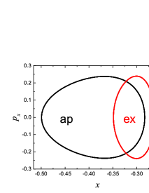
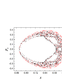
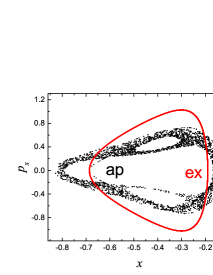
Fig. 1: Phase-space structures on the Poincaré section $y=0$ with $v_{y}>0$, which are described by RKF89 solving the PN circular restricted three-body problem. ap represents the approximate Euler-Lagrange equations, and ex stands for the exact Euler-Lagrange equations. The parameters are $\mu_{2}=0.001$, $\mu_{1}=1-\mu_{2}$, $C_{j}=3.07$ and $c=100$, and the initial conditions are $y=v_{x}=0$. The other initial conditions and parameters are (a): $a=1$ and $x=0.35$; (b): $a=10$ and $x=0.28$; (c): $a=1$ and $x=0.4895$; (d): $a=2$ and $x=0.687$. The approximate equations and the exact ones yield the same regular torus in panel (a) and same chaotic solutions in panel (c). They have different regular tori in panel (b). In panel (d), the approximate equations correspond to chaos, whereas the exact equations exhibit the regularity.

An eighth- and ninth-order Runge-Kutta-Fehlberg integrator [RKF89] with adaptive step sizes is used to provide high-precision reference solutions for evaluating the numerical performance of low order methods such as EM4. With the aid of this integrator, the solutions of the exact Euler-Lagrange equations (11), (12), (29) and (30) and the approximate Euler-Lagrange equations (32) can be obtained. In this way, phase-space structures of four orbits in the two sets of equations are described on the Poincaré section $y=0$ with $v_{y}>0$ in Fig. 1. Here, the initial conditions are $y=v_{x}=0$, and the parameters are $\mu_{2}=0.001$, $\mu_{1}=1-\mu_{2}$ and $C_{j}=3.07$. As is above-mentioned, $c$ is used as a free parameter. When the parameters $a$ and $c$ and the starting value of $x$ are considered, the initial value of $v_{y}>0$ is solved from Eq. (31).

The two sets of equations have almost the same Kolmogorov-Arnold-Moser (KAM) torus for the starting value $x=0.35$ with parameters $c=100$ and $a=1$ in Fig. 1(a). This KAM torus indicates the regularity of the integrated orbit. Although the two sets of equations yield regular KAM tori for the starting value $x=0.28$ with parameters $a=10$ and $c=100$ in Fig. 1(b), the two tori are typically different. For the initial value $x=0.4895$ with parameters $c=100$ and $a=1$ in Fig. 1(c), the exact equations and the approximate ones produce approximately same chaotic solutions with many points filled with areas. For the initial value $x=0.687$ with $c=100$ and $a=2$ in Fig. 1(d), chaos occurs in the approximate equations, whereas does not in the exact equations. Figs. 1 (b) and (d) show that the approximate equations and the exact ones have distinct phase-space structures, i.e., distinct solutions. This supports the results of [29, 30] again. Which of the approximate Euler-Lagrange equations and the exact ones can give correct solutions to the Lagrangian (25)? The exact Euler-Lagrange equations can without question. Thus, they are used as a test model in the following numerical simulations.

RKF89 can significantly improve the accuracy, as can be verified by comparison with lower-order integrators like EM4. However, the improved accuracy requires that RKF89 be more computationally demanding than these lower-order integrators for long-term integrations. If the lower-order integrators can provide reliable results, they should be employed to study the trajectories and to detect the chaotical behavior. In view of this point, three fourth-order integrators are compared with EM4. They are an implicit symplectic method (IM4) consisting of three second-order implicit midpoint rules [35], a Runge-Kutta integrator (RK4), and a Gauss-Runge-Kutta (GRK) implicit symplectic method [34, 37-39]. The four methods EM4, IM4, GRK and RK4 can yield the same phase-space structures to the four orbits in Fig. 1 for short integration times. When the integrations are long enough, the three methods EM4, IM4 and GRK still have the same phase-space structures as those of Fig. 1, but RK4 does not have.

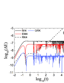
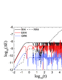
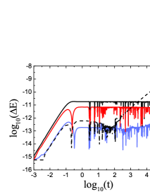
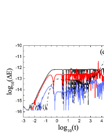
Fig. 2: Relative energy errors for four algorithms solving the exact Euler-Lagrange equations. (a) The orbit is the regular orbit of Fig. 1(a). (b) The orbit is the chaotic orbit of Fig. 1(c). The step size is $h=0.01$ in panels (a) and (b). Panels (c) and (d) that adopt a smaller step size $h=0.001$ correspond to panels (a) and (b), respectively.

When the step size is chosen as $h=0.01$, Figs. 2 (a) and (b) plot relative energy errors of the regular orbit in Fig. 1(a) and the chaotic orbit in Fig. 1(c). The relative energy errors are calculated by $\Delta E=|(E_{t}-E_{0})/E_{0}|$, where $E_{0}$ is the energy in Eq. (4) at time 0 and $E_{t}$ stands for the energy calculated at integration time $t$. The errors remain bounded for the three geometric integrators EM4, IM4 and GRK, whereas grow with time for RK4. They are about orders of $10^{-12}$ to $10^{-6}$ for EM4, IM4 and GRK, and $10^{-12}$ to $10^{-5}$ for RK4. The accuracies are good and acceptable in the machine’s double precision. The methods with the errors from small to large are GRK, EM4, IM4 and RK4. The calculations in the chaotic case (Fig. 2(b)) appear to be more accurate than in the regular ones (Fig. 2(a)). An explanation to this result is given here. Based on the theory of numerical calculations, the truncation error in energy is approximately estimated by $(h/T)^{k}$ for a $k$th-order symplectic method, and it in solutions is estimated by $(h/T)^{k+1}$, where $T$ is an orbital period. The period for the ordered orbit in Fig. 2(a) is $T\approx 5.11$. Although the orbit is chaotic in Fig. 2(b), it has an approximate average period $T\approx 7.91$. For a given time step, the energy accuracies get higher with an increase of the orbital periods. Thus, it is reasonable that the energy accuracies for the regular case in Fig. 2(a) are poorer than those for the chaotic case in Fig. 2(b). However, the solutions’ accuracies should be better for former case than those for the latter case because the solutions in the chaotic case exhibit exponentially sensitive dependence on the initial conditions. When a smaller step size $h=0.001$ is used in Figs. 2 (c) and (d), the energies have higher accuracies and are accurate to orders of $10^{-15}\sim 10^{-11}$ for the three geometric integrators. To ensure such higher enough accuracies, we adopt the smaller step size $h=0.001$ in the PN circular restricted three-body problem.

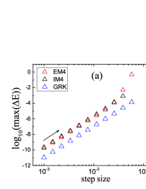
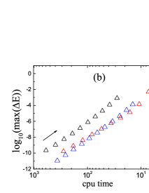
Fig. 3: Efficiency plots for the three methods EM4, GRK and IM4. The initial condition and parameters are $c=100$, $a=1$ and $x=0.28$. The maximum relative energy error for each time step and algorithm is obtained after the integration time $t=10^{5}$. The dependence of relative energy error on the step size in (a) shows that EM4 and IM4 have almost the same accuracies for a given step size. The dependence of relative energy error on CPU time (unit: second) in (b) indicates that EM4 takes less computational cost than IM4 and is almost the same computational cost as GRK for a given accuracy.

It is worth noticing the differences in computations among the three geometric methods EM4, IM4 and GRK. The position r and velocity v must be solved in terms of the iteration method in IM4 and GRK, but only the solutions of v need iterations in EM4. This seems to show that the computational cost for EM4 is less than for IM4 or GRK. To check the result, we plot computational efficiencies in Fig. 3. The test orbit is that of Fig. 1(a). A series of step sizes $h=10^{-3}$, $10^{-3}\times 1.2$, $10^{-3}\times 1.2^{2}$, $10^{-3}\times 1.2^{3}$, $\cdots$ are considered. When one of the time steps is given, the maximum relative energy errors for the three schemes during the integration time $t=10^{5}$ are drawn in Fig. 3(a). GRK exhibits the best accuracy. EM4 and IM4 are almost the same in the accuracies. Each of the maximum errors corresponding to CPU time is shown in Fig. 3(b). When the three methods use different time steps and provide the same accuracy, EM4 or GRK takes less CPU time than IM4. EM4 and GRK take almost the same CPU times. Given CPU time, the accuracy of EM4 is two or three orders of magnitude better than that of IM4, and is approximately the same as that of GRK. Obviously, the efficiency of EM4 is superior to that of IM4. In other words, EM4 needs less computational cost than IM4 and GRK when the time step and integration time are fixed.

III.3 Dependence of chaos on the initial conditions and parameters

Considering reliable computational accuracy and high efficiency for given time step and integration time, we use EM4 to study the orbital dynamical behavior of orbits in the exact equations. Apart from the technique of Poincaré sections, Lyapunov exponents [62] and fast Lyapunov indicators (FLIs) [63-65] are often used to distinguish between the regularity and chaoticity of bounded orbits. The FLI is defined as

$$FLI=\log_{10}\frac{d(t)}{d(0)},$$ (33)

where $d(t)$ and $d(0)$ are the distances between two nearby trajectories at times $t$ and 0. The initial separation $d(0)=10^{-9}$ is a sufficient choice. The FLI with two nearby trajectories proposed in Ref. [63] is originated from a modified version of the FLI with two tangent vectors given in Refs. [64, 65], and is also from a modified version of the Lyapunov exponents with two nearby trajectories [62]. For convenience of analytical discussion, the original FLI (denoted by $\delta=\ln(d(t)/d(0))$) is adopted. If $\delta=e^{\ln t}$, then $d(t)=d(0)e^{t}$. This indicates that the distance $d(t)$ grows exponentially with time $t$. This characteristic is just the description of the largest Lyapunov exponent, which shows the chaoticity of a bounded orbit. If $\delta=k\ln t$, then $d(t)=d(0)t^{k}$. This indicates that the distance $d(t)$ grows in a power law of time $t$. It is the characteristic of a regular bounded orbit. There are two particular cases about the relation $\delta=k\ln t$. When $k=1$, $\delta=\ln t$ corresponds to regular orbits. Lukes-Gerakopoulos et al. [67] have shown that $\delta$ behaves like $\delta=k\ln t$ for a transient time before the exponential growth of weak chaotic orbits takes over. An exponential increase of the distance is much larger than a polynomial increase of the distance. Such typically different ratios of growth of FLIs with time are used to detect chaos from order. An exponential growth of FLI with time $\log_{10}t$ indicates the chaoticity of a bounded orbit, but a linear growth of FLI with time shows the regularity of a bounded orbit.

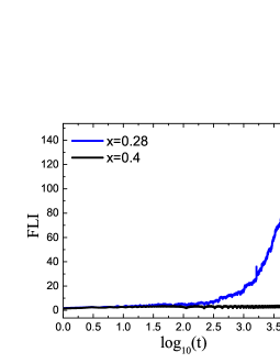
Fig. 4: Fast Lyapunov indicators (FLIs) of two orbits. The parameters are $c=100$, $a=1$ and $c_{j}=3.07$.

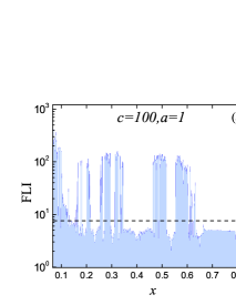
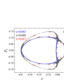
Fig. 5: (a) Dependence of FLIs on the initial values $x$. (b) Poincaré sections for ordered orbits with $x=0.665$ corresponding to FLI=5.3 and $x=0.667$ (FLI=5.2), and a chaotic orbit with $x=0.666$ (FLI=21.1).

The FLIs of two orbits with initial values $x=0.4$ and $x=0.28$ are shown in Fig. 4. The parameters and other initial conditions (except the initial value $v_{y}$) are those of Fig. 1(a). The initial value $x=0.4$ corresponds to the regularity, and the initial value $x=0.28$ indicates the chaoticity. It is found that 7.5 is a threshold value of FLIs between the regular and chaotic cases when the integration time reaches $t=10^{4}$. The FLIs larger than 7.5 indicate the presence of chaos, whereas the FLIs no more than the threshold mean the presence of order. The technique of FLIs is convenient to trace a transition from order to chaos with a parameter or an initial condition varying. Fig. 5 draws the dependence of FLIs on the initial values $x$. The parameters and other initial conditions (except the initial value $v_{y}$) are the same as those of Fig. 1(a). The initial values $x$ corresponding to order and chaos are shown clearly. Two larger regular intervals for the onset of order are $0.346\leq x\leq 0.485$ and $0.667\leq x\leq 0.805$. There are four larger chaotic intervals: $0.254\leq x\leq 0.295$, $0.3125\leq x\leq 0.3455$, $0.463\leq x\leq 0.56185$, and $0.5545\leq x\leq 0.6335$. A number of smaller regular or chaotic intervals are also present. Taking the FLIs neighboring $x=0.666$ as examples, we focus on the transition between order and chaos. FLI=5.3 for $x=0.665$ and FLI=5.2 for $x=0.667$ correspond to the regular case, but FLI=21.1 for $x=0.666$ corresponds to the chaotic case. The regularity and chaoticity are shown through the Poincaré sections in Fig. 5(b).

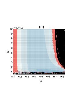
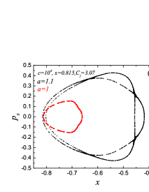
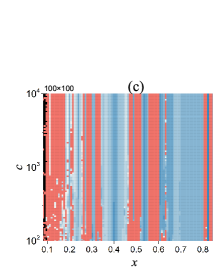
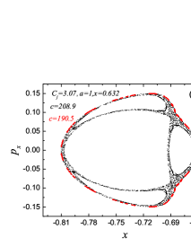
Fig. 6: (a) Dependence of FLIs on the parameter $a$ and initial value $x$. $c=10^{4}$ is fixed. Red: chaos, Black: unstable, other: order. (b) Poincaré sections for the regular case of $x$=0.815 and $a=1$ with FLI=5.59 and the chaotic case of $x$=0.815 and $a=1.1$ with FLI=46.88. (c) Dependence of FLIs on the parameter $c$ and initial value $x$. $a=1$ is fixed. (d) Poincaré sections for the regular case of $x$=0.632 and $c=190.5$ with FLI=5.91 and the chaotic case of $x$=0.632 and $c=208.9$ with FLI=12.48.

Fig. 6(a) describes the dependence of FLIs on parameter $a$ and the initial value $x$. Given $c=10^{4}$, $a$ runs from 1 to 10 with an interval of 0.1, and $x$ ranges from 0.1 to 0.9 with an interval of 0.01. The other parameters and initial conditions (except the initial value $v_{y}$) are still those of Fig. 1(a). A great two-dimensional space of $a$ and $x$ corresponds to the regularity of bounded orbits. There are larger unstable regions colored Black. Many smaller areas for the chaoticity of bounded orbits exist. Chaos mainly occurs in the neighbourhood of $x=0.1$ or $a=1$. Of course, chaos also easily appears in the boundary regions between the ordered and unstable regions. For example, the orbit is ordered for $a=1$ and $x=0.815$ with FLI=5.59, while chaotic for $a=1.1$ and $x=0.815$ with FLI=46.88, as can be seen from the Poincaré sections in Fig. 6(b). In Fig. 6(c) with $a=1$, $c$ ranges from 100 to 10000, and $x$ runs from 0.1 to 0.9. There are many larger two-dimensional spaces of $c$ and $x$ for the onset of order and chaos. Thinner unstable regions can be met in the neighbourhood of $x=0.1$ or $x=0.9$. Fig. 6(d) shows that order exists for $x=0.632$ and $c=190.5$ with FLI=5.91, while chaotic for $x=0.632$ and $c=208.9$ with FLI=12.48.

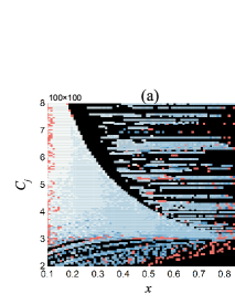
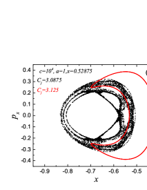
Fig. 7: (a) Dependence of FLIs on the parameter $C_{j}$ and initial value $x$. (b) Poincaré sections for two orbits.

When $a=1$ and $c=10^{4}$ are given in Fig. 7(a), the Jacobi constant $C_{j}$ runs from 2 to 8 with an interval of 0.06, and the initial position $x$ is also considered from 0.1 to 0.9. The other parameters and initial positions are those of Fig. 1(a). The values of $C_{j}$ and $x$ are more for the regular case than for the chaotic case, whereas less than for the unstable case. Fig. 7(b) displays that the orbit is ordered for $C_{j}=3.125$ and $x=0.52875$ with FLI=4.89, while chaotic for $C_{j}=3.0875$ and $x=0.52875$ with FLI=111.06.

Two points are illustrated here. The dynamical results obtained from EM4 in Figs. 4-7 are consistent with those given by RKF89. In addition, the technique of FLIs can sensitively distinguish between the regular and chaotic two cases. It is effective to trace the transition from order to chaos with a variation of one or two initial conditions and parameters in Figs. 5-7.

IV Spinning compact binaries

A PN Lagrangian system of two spinning black holes is introduced simply in Sect. 4.1. When the spins are expressed in a set of canonical coordinates, the symplectic-like integrator EM4 is applied to the exact Euler-Lagrange equations and its performance is evaluated in Sect. 4.2. The orbital dynamics of order and chaos in the exact Euler-Lagrange equations are investigated in Sect. 4.3.

IV.1 Dynamical equations

Let us consider two black holes with masses $M_{1}$ and $M_{2}$. They have the total mass $M=M_{1}+M_{2}$, the reduced mass $\mu=M_{1}M_{2}/M$, and $\nu=\mu/M$. Body 2 relative to body 1 has position $\mathbf{r}$ and velocity $\mathbf{v}$. We take $r=|\mathbf{r}|$, $\mathbf{n}=\mathbf{r}/r$, and $\dot{r}=\mathbf{n}\cdot\mathbf{v}$. The two bodies evolve according to the PN Lagrangian in the ADM coordinates [56, 66]:

$$\mathcal{L}(\mathbf{r},\mathbf{v},\mathbf{S}_{1},\mathbf{S}_{2})=\mathcal{L}_{O}+\mathcal{L}_{S}.$$ (34)

$\mathcal{L}_{O}$ is an orbital part with the following expression

$$\mathcal{L}_{O}=\mathcal{L}_{N}+\frac{1}{c^{2}}\mathcal{L}_{1PN}+\frac{1}{c^{4}}\mathcal{L}_{2PN},$$ (35)

where the Newtonian term $\mathcal{L}_{N}$ and the 1PN and 2PN contributions $\mathcal{L}_{1PN}$ and $\mathcal{L}_{2PN}$ are

$$\mathcal{L}_{N}=\frac{1}{r}+\frac{\mathbf{v}^{2}}{2},$$ (36)

$$\mathcal{L}_{1PN}= \frac{\mathbf{v}^{4}}{8}-\frac{3\nu\mathbf{v}^{4}}{8}-\frac{1}{2r^{2}}$$ (37)

$$+\frac{1}{r}\left(\frac{\nu{\dot{r}}^{2}}{2}+\frac{3\mathbf{v}^{2}}{2}+\frac{\nu\mathbf{v}^{2}}{2}\right),$$

$$\mathcal{L}_{2PN}= \frac{\mathbf{v}^{6}}{16}-\frac{7\nu\mathbf{v}^{6}}{16}+\frac{13\nu^{2}\mathbf{v}^{6}}{16}$$ (38)

$$+\frac{1}{r}\left(\frac{3\nu^{2}\dot{r}^{4}}{8}+\frac{\nu\dot{r}^{2}\mathbf{v}^{2}}{2}-\frac{5\nu^{2}\dot{r}^{2}\mathbf{v}^{2}}{4}\right.$$

$$\left.+\frac{7\mathbf{v}^{4}}{8}-\frac{3\nu\mathbf{v}^{4}}{2}-\frac{9\nu^{2}\mathbf{v}^{4}}{8}\right)$$

$$+\frac{1}{r^{2}}\left(\frac{3\nu\dot{r}^{2}}{2}+\frac{3\nu^{2}\dot{r}^{2}}{2}+2\mathbf{v}^{2}-\nu\mathbf{v}^{2}+\frac{\nu^{2}\mathbf{v}^{2}}{2}\right)$$

$$+\frac{1}{r^{3}}\left(\frac{1}{4}+\frac{3\nu}{4}\right).$$

The two bodies spin according to the spin effects

$$\mathcal{L}_{S}=\frac{1}{c^{3}}\mathcal{L}_{1.5SO}+\frac{1}{c^{4}}\mathcal{L}_{2SS},$$ (39)

where the 1.5PN spin-orbit coupling $\mathcal{L}_{1.5SO}$ and the 2PN spin-spin effect $\mathcal{L}_{2SS}$ [26] are

$$\mathcal{L}_{1.5SO}=\frac{\nu}{r^{3}}\mathbf{v}\cdot\left[\mathbf{r}\times\left(\gamma_{1}\mathbf{S_{1}}+\gamma_{2}\mathbf{S_{2}}\right)\right],$$ (40)

$$\mathcal{L}_{2SS}=-\frac{\nu}{2r^{3}}\left[\frac{3}{r^{3}}\left(\mathbf{S_{0}}\cdot\mathbf{r}\right)^{2}-\mathbf{S_{0}}^{2}\right].$$ (41)

Note that $\gamma_{1}=2+3/(2\beta)$, $\gamma_{2}=2+3\beta/2$, and $\mathbf{S_{0}}=\left(1+1/\beta\right)\mathbf{S_{1}}+\left(1+\beta\right)\mathbf{S_{2}}$, where the mass ratio is $\beta=M_{2}/M_{1}$. Eqs. (34)-(41) are dimensionless through a series of scale transformations: $\mathbf{r}\rightarrow GM\mathbf{r}$, $t\rightarrow GMt$, $\mathbf{S_{i}}\rightarrow G\mu M\mathbf{S_{i}}~{}(i=1,2)$, and $\mathcal{L}\rightarrow\mu\mathcal{L}$. $G$ uses a geometric unit $G=1$.

The Hamiltonian (7) for the PN Lagrangian (34) reads

$$\mathcal{H}(\mathbf{r},\mathbf{v},\mathbf{S}_{1},\mathbf{S}_{2})=\mathbf{v}\cdot\mathbf{p}-\mathcal{L}(\mathbf{r},\mathbf{v},\mathbf{S}_{1},\mathbf{S}_{2}),$$ (42)

where the momentum $\mathbf{p}$ is still defined in Eq. (1) by

$$\mathbf{p}=\frac{\partial}{\partial\mathbf{v}}\mathcal{L}(\mathbf{r},\mathbf{v},\mathbf{S}_{1},\mathbf{S}_{2}).$$ (43)

As is aforementioned, $\mathbf{v}$ in Eq. (43) can be expressed as a function of $\mathbf{r}$, $\mathbf{p}$, $\mathbf{S}_{1}$ and $\mathbf{S}_{2}$. The higher-order terms are truncated in general if $\mathbf{v}$ is expressed in terms of $\mathbf{p}$. However, $\mathbf{v}$ in Eq. (42) has no such operation and is still remained. This means that Eq. (42) is only a formal Hamiltonian but is not a standard Hamiltonian (note that the standard Hamiltonian should be a function of coordinates and momenta rather than a function of coordinates and velocities). That is to say, the formal Hamiltonian, as a function of $\mathbf{r}$, $\mathbf{v}$, $\mathbf{p}$, $\mathbf{S}_{1}$ and $\mathbf{S}_{2}$, comes directly from the Legendre transformation of the Lagrangian and has no terms truncated. Thus, it is exactly equivalent to this Lagrangian. The PN Lagrangian (34) has four integrals of motion, which involve the energy integral

$$E=\mathcal{H}(\mathbf{r},\mathbf{v},\mathbf{S}_{1},\mathbf{S}_{2}),$$ (44)

and the total angular momenta

$$\mathbf{J}=\mathbf{r}\times\mathbf{p}+\mathbf{S}_{1}+\mathbf{S}_{2}.$$ (45)

Because no terms are truncated when the formal Hamiltonian is obtained from the Lagrangian, the energy is an exact integral in the Lagrangian.

Apart from the four integrals, the two spin lengths $S_{i}=\chi_{i}M^{2}_{i}/(\mu M)~{}(0\leq\chi_{i}\leq 1)$ also remain constant. Using the constant spin lengths, Wu $\&$ Xie [33] introduced the canonical spin coordinates $(\theta_{i},\xi_{i})$ as follows:

$$\bm{S}_{i}=\left(\begin{array}[]{l}\rho_{i}\cos\theta_{i}\\ \rho_{i}\sin\theta_{i}\\ \xi_{i}\end{array}\right),$$ (46)

where $\rho_{i}$ are expressed as

$$\rho_{i}=\sqrt{S^{2}_{i}-\xi^{2}_{i}}.$$ (47)

Now, the Hamiltonian can be expressed in terms of ten independent phase space variables, consisting of five degrees of freedom (i.e., generalized coordinates) $(\mathbf{r},\theta_{1},\theta_{2})$ and five conjugate momenta $(\mathbf{p},\xi_{1},\xi_{2})$. These independent variables evolve by satisfying the Hamiltonian canonical equations of motion:

$$\dot{\mathbf{r}}_{i} = \frac{\partial\mathcal{H}}{\partial\mathbf{p}}=\mathbf{v},$$ (48)

$$\dot{\theta}_{i} = \frac{\partial\mathcal{H}}{\partial\xi_{i}}=-\frac{\partial\mathcal{L}}{\partial\mathbf{S}_{i}}\cdot\frac{\partial\mathbf{S}_{i}}{\partial\xi_{i}};$$ (49)

$$\dot{\mathbf{p}} = -\frac{\partial\mathcal{H}}{\partial\mathbf{r}}=\frac{\partial\mathcal{L}}{\partial\mathbf{r}},$$ (50)

$$\dot{\xi}_{i} = -\frac{\partial\mathcal{H}}{\partial\mathbf{\theta}_{i}}=\frac{\partial\mathcal{L}}{\partial\mathbf{S}_{i}}\cdot\frac{\partial\mathbf{S}_{i}}{\partial\theta_{i}}.$$ (51)

$\mathbf{r}$ and $\mathbf{p}$ are a pair of canonical variables. So are $\theta_{i}$ and $\xi_{i}$. After the solutions $(\textbf{r},\theta_{1},\theta_{2},\textbf{p},\xi_{1},\xi_{2})$ are solved from Eqs. (48)-(51), v is calculated iteratively in terms of Eq. (43). Eqs. (48)-(51) with Eq. (43) are strictly derived from the Lagrangian (34) and exactly conserve the energy (44). In this case, the four algorithms EM4, IM4, GRK and RK4 are available for the exact Euler-Lagrange equations (48)-(51). The solutions are not given analytically because the existence of the four integrals including the total energy and the total momenta in the 10-dimensional phase space determines the non-integrability of the formal PN Hamiltonian (or Lagrangian) formulation.

Another consideration is that the total accelerations to the 2PN order can be derived from the Euler-Lagrange equations of the Lagrangian (34) and are written as

$$\frac{d\mathbf{v}}{dt}=\frac{\partial\mathcal{L}}{\partial\mathbf{r}}+\frac{\tilde{\mathbf{a}}_{1PN}}{c^{2}}+\frac{\tilde{\mathbf{a}}_{1.5SO}}{c^{3}}+\frac{\tilde{\mathbf{a}}_{2PN}}{c^{4}}+\cdots.$$ (52)

The PN accelerations such as $\tilde{\mathbf{a}}_{1PN}$ in the right-hand side of Eq. (52) are originated from the derivative of momenta (43) with respect to time (i.e., $d\mathbf{p}/dt$) in the Euler-Lagrange equations. Because the PN terms higher than the 2PN terms are dropped in the total accelerations, Eq. (52) with Eqs. (48), (49) and (51) is the approximate equations of the Lagrangian (34). Of course, such approximate equations do not exactly conserve the energy (44).

It is worth pointing out that the differences in the PN contributions (including the spin effects) between the two sets of equations are apparent. To show the differences, we rewrite Eqs. (43) and (5) of the exact equations as

$$\mathbf{\dot{v}} = \frac{\partial\mathcal{L}}{\partial\mathbf{r}}+\mathbf{f}_{1PN}(\mathbf{r},\mathbf{v},\mathbf{\dot{v}})+\mathbf{f}_{2PN}(\mathbf{r},\mathbf{v},\mathbf{\dot{v}})$$ (53)

$$+\mathbf{f}_{SO}(\mathbf{r},\mathbf{v},\mathbf{S}_{1},\mathbf{S}_{2},\mathbf{\dot{S}}_{1},\mathbf{\dot{S}}_{2}),$$

where $\mathbf{f}_{1PN}$, $\mathbf{f}_{2PN}$ and $\mathbf{f}_{SO}$ are functions associated to the PN accelerations. This equation is an implicit equation with respect to the acceleration $\mathbf{\dot{v}}$. When $\mathbf{\dot{v}}=-\mathbf{r}/r^{3}$ (i.e., the Newtonian acceleration is given to $\mathbf{\dot{v}}$) and $\mathbf{\dot{S}}_{1}=\mathbf{\dot{S}}_{2}=0$ in the right-hand side of Eq. (53), the approximate equations (52) is obtained. However, these approximations are not given to the exact equations. If $\mathbf{\dot{v}}$ takes the 1PN orbital contribution, 1.5PN spin-orbit term, 2PN orbital term and 2PN spin-spin coupling in the function $\mathbf{f}_{1PN}$, then $\mathbf{f}_{1PN}$ includes the 2PN orbital contribution, 2.5PN spin-orbit term, 3PN orbital term and 3.5PN spin-orbit coupling. In this case, $\mathbf{f}_{2PN}$ contains the 3PN orbital contribution, 3PN spin-spin effect, 4PN orbital term and 4PN spin-spin coupling. If $\mathbf{\dot{S}}_{1}$ and $\mathbf{\dot{S}}_{2}$ in the function $\mathbf{f}_{SO}$ are Eqs. (49) and (51), then $\mathbf{f}_{SO}$ has 3PN spin-spin coupling and 3.5PN spin-orbit interaction. Thus, besides the terms in the approximate equations (52), many other terms such as the 2.5PN spin-orbit coupling and the 3PN spin-spin contribution are included in the exact equations (53). The 2.5PN spin-orbit and 3PN spin-spin contributions are implicitly hidden in the exact equations, but are absent in the approximate equations.

IV.2 Numerical tests

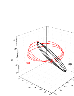
Fig. 8: Three-dimensional orbits, described by RKF89 solving the approximate Euler-Lagrange equations and the exact ones of spinning compact binaries.

Same as $G$, the speed of light $c$ also takes the geometric unit $c=1$. The parameters are given by $\chi_{1}=\chi_{2}=1$ and $\beta=4$. The initial conditions are chosen as $x=70$, $y=0$, $z=0$, $p_{x}=p_{z}=0$, and $p_{y}=\sqrt{(1-e)/x}$ with initial eccentricity $e=0.16$. The initial canonical spin variables are given by $\theta_{1}=\theta_{2}=\pi/2$, $\xi_{1}=0.1$ and $\xi_{2}=0.95$. When RKF89 is used, the approximate Euler-Lagrange equations and the exact ones have different three-dimensional orbits after a time of integration in Fig. 8. As is mentioned above, the exact Euler-Lagrange equations should be chosen as the equations of motion for the Lagrangian (34).

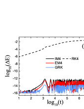
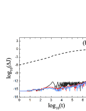
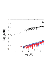
Fig. 9: Relative errors in the energy (a), angular momentum (b) and position (c) for the four algorithms acting on the coherent PN Euler-Lagrange equations. The initial conditions are $x=70$, $p_{y}=\sqrt{(1-e)/x}$ with $e=0.16$, $\theta_{1}=\theta_{2}=\pi/2$, $\xi_{1}=0.1$ and $\xi_{2}=0.95$. The parameters are $\beta=4$ and $\chi_{1}=\chi_{2}=1$.

Now, RKF89 is replaced with one of the four algorithms EM4, IM4, GRK and RK4. The step size $h=1$ is fixed. Fig. 9 plots the relative energy errors $\Delta E$, relative total angular momentum errors $\Delta J$ and relative position errors $\Delta R$ for the four integrators. Here, $\Delta E=|(E_{t}-E_{0})/E_{0}|$, and $\Delta J=|\textbf{J}_{t}-\textbf{J}_{0}|/|\textbf{J}_{0}|$, where $\textbf{J}_{0}$ is the total angular momenta (45) at time 0 and $\textbf{J}_{t}$ denotes the total angular momenta calculated at integration time $t$. The positions calculated by these methods at time $t$ are $\textbf{r}_{E}$ for EM4, $\textbf{r}_{I}$ for IM4, $\textbf{r}_{G}$ for GRK, and $\textbf{r}_{R}$ for RK4. The higher-precision method RKF89 is used to provide reference solutions such as position $\textbf{r}_{F}$. In this way, the relative position errors between RKF89 and EM4 can be computed by $\Delta R=|\textbf{r}_{F}-\textbf{r}_{E}|/|\textbf{{r}}_{F}|$. The position errors between RKF89 and one of IM4, GRK and RK4 are also calculated in this similar way. The three geometric methods EM4, IM4 and GRK give no secular growth to the errors in the total energy and the total angular momenta. In other words, they conserve the total energy and the total angular momenta. They have no dramatic but minor differences in the accuracies, and their accuracies are almost approximate to the machine’s precision. In the energy accuracies, GRK is slightly better than EM4 or IM4; EM4 and IM4 are approximately the same. In the angular momentum accuracies, EM4 and GRK are basically the same, and are slightly superior to IM4. However, RK4 does not conserve the total energy and the total angular momenta, and exhibits the poorest accuracies. The three methods EM4, IM4 and GRK are almost the same in the relative position errors as the integration lasts. The position errors for EM4, IM4 and GRK are several orders of magnitude smaller than those for RK4.

The numerical tests show that the three geometric integrators exhibit good long-term performance in the conservation of energy and angular momentum, but RK4 exhibits poor long-term performance. For given time step and integration time, EM4 is superior to IM4 and GRK in computational efficiency.

IV.3 Orbital dynamics

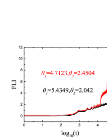
Fig. 10: FLIs of two orbits in the exact equations. The initial conditions are the same as those in Fig. 9, but the initial eccentricity $e=0.66$ and initial spin angles $\theta_{1}$ and $\theta_{2}$ are different. For the initial spin angles $\theta_{1}=5.4349$ and $\theta_{2}=2.042$ with FLI= 2.56, the dynamics is regular. However, the dynamics is chaotic for the initial spin angles $\theta_{1}=4.7123$ and $\theta_{2}=2.4504$ with FLI= 10.48.

EM4 combined with the technique of FLIs is employed to explore the dynamical behavior of orbits. The initial conditions are the same as those in Fig. 9, except for the initial eccentricity $e=0.66$ and the initial spin angles $\theta_{1}$ and $\theta_{2}$. The initial spin angles $\theta_{1}=5.4349$ and $\theta_{2}=2.042$ with FLI= 2.56 yield a regular solution in Fig. 10. However, the initial spin angles $\theta_{1}=4.7123$ and $\theta_{2}=2.4504$ with FLI= 10.48 exhibit a chaotic solution. The FLIs larger than 7.5 indicate the chaoticity, whereas the FLIs no more than than 7.5 indicate the regularity when the integration time reaches $t=10^{5}$. The performance of this integrator in the conservation of energy and angular momenta is independent of the regularity or chaoticity of orbits.

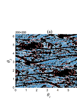
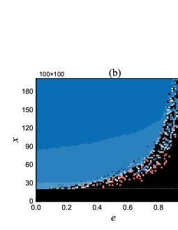
Fig. 11: (a) Dynamical structures by using the FLIs to scan the initial spin angles $\theta_{1}$ and $\theta_{2}$. (b) To scan the initial eccentricities $e$ and initial separations $x$. Red: chaos, Black: unstable, Blue: order.

Using the FLIs, we can classify the two-dimensional space of initial spin angles according to different orbital dynamical features in Fig. 11(a). Our method is described here. The initial conditions and parameters are the same as those in Fig. 10. The initial spin angles $\theta_{1}$ and $\theta_{2}$ range from 0 to $2\pi$ with an interval of $0.01\times\pi$. The FLI for each pair of $\theta_{1}$ and $\theta_{2}$ is obtained after the integration time $t=10^{5}$. Based on the FLIs, the initial spin angles $\theta_{1}$ and $\theta_{2}$ can be divided into three regions: regular region of bounded orbits, chaotic region of bounded orbits and unstable region. A number of initial spin angles correspond to the regularity, and many initial spin angles colored Red indicate the presence of chaos. There are a lot of initial spin angles colored Black leading to the instability. No rule on the transition from order to chaos can be given as the initial spin angles are varied. Fig. 11(b) relates to the dependence of FLIs on the initial eccentricities $e$ and initial separations $x$ with mass ratio $\beta=3$. The other initial conditions and parameters are the same as those of Fig. 9. There are two main parts. The largest region colored Blue corresponds to order. The larger region colored Black shows that none of the orbits is stable below the horizon line $x=21.8$. Only a small number of values of $x$ and $e$ on the boundary between order and instability indicate the onset of chaos. For instance, the orbit with $e=0.75$ and $x=65$ having FLI=12.3 is chaotic. The result concluded in Fig. 11(b) is that the orbits become unstable as the initial eccentricities increase or the initial separations decrease, whereas stable and regular as the initial separations increase.

Some explanations to the above results are given here. The exact Euler-Lagrange equations are conservative, integrable and nonchaotic when the two bodies do not spin. However, when the two bodies are spinning, the spin contributions lead to the nonintegrability and probable chaoticity of the exact equations. The spin effects play an important role in the onset of chaos. As is claimed above, the 1.5PN spin-orbit and 2PN spin-spin contributions are explicitly included in the exact equations, and the 2.5PN spin-orbit and 3PN spin-spin contributions are implicitly hidden. The 2.5PN spin-orbit and 3PN spin-spin contributions hidden in the exact equations would easily induce the instability or chaoticity of the solutions for the exact equations. Larger initial eccentricities and smaller initial separations $x$ cause an increase of the spin effects, and therefore chaos or instability is easily induced.

V Conclusion

A PN Lagrangian formalism can be exactly equivalent to the same order PN formal Hamiltonian (7), where the positions and momenta are phase-space variables but velocities are implicit functions of the positions and momenta. Such a formal Hamiltonian seems to explicitly depend on the positions, velocities and momenta. Because these velocities are solved iteratively from the algebraic equations of the momenta defined by the Lagrangian, this Hamiltonian is still a function of the positions and momenta. The Lagrangian formalism is not exactly equivalent to the same order PN standard Hamiltonian (5), which is a function of the positions and momenta. The canonical equations for the formal PN Hamiltonian (7) must strictly conserve the Hamiltonian quantity, i.e., energy. They are the coherent or exact PN Euler-Lagrange equations of motion.

Doubling the phase-space variables including the positions and momenta in the formal Hamiltonian, we introduce a new Hamiltonian in extended phase space. This new Hamiltonian consists of two parts: one of which is equal to the original formal Hamiltonian depending on the original positions and the new momenta with the new velocities, and another of which is equal to the original Hamiltonian depending on the original momenta and the new positions with original velocities. The solutions of Hamilton’s canonical equations for the two parts of the new Hamiltonian are used to design the standard second-order symplectic leapfrog methods and fourth-order symplectic schemes. When these algorithms are combined with the midpoint permutations, the extended phase-space symplectic-like integrators become easily available for the coherent PN Euler-Lagrange equations. In the course of numerical integrations, the velocities must be solved iteratively.

Numerical tests show that a fourth-order extended phase-space symplectic-like method exhibits good long-term stabilizing error behavior in energy or angular momentum, as fourth-order implicit symplectic method and Gauss-Runge-Kutta scheme do. The former method takes less computational cost than the latter integrators for given time step and integration time. This good numerical performance of the extended phase-space method is independent of the regularity or chaoticity of orbits. Because of such good performance, the extended phase-space symplectic-like method with the technique of FLIs is well applicable to studying the effects of the parameters and initial conditions on the orbital dynamics of the coherent Euler-Lagrange equations for a post-Newtonian circular restricted three-body problem. The parameters and initial conditions corresponding to order, chaos and instability are found. They are also applied to trace the effects of the initial spin angles, initial separations and initial orbital eccentricities on the dynamics of the coherent post-Newtonian Euler-Lagrange equations of spinning compact binaries. As a result, the initial spin angles, initial separations and initial orbital eccentricities for the presence of order, chaos and instability are obtained. Larger initial eccentricities and smaller initial separations easily induce the occurrence of chaos or instability.

References

- (1) B. P. Abbott, et al., Phys. Rev. Lett. 116, 061102 (2016).
- (2) R. Abbott, et al., Phys. Rev. Lett. 125, 101102 (2020).
- (3) V. de Luca, V. Desjacques, et al. Phys. Rev. Lett. 126, 051101 (2021).
- (4) J. Levin, Phys. Rev. Lett. 84, 3515 (2000).
- (5) N. J. Cornish and J. Levin, Phys. Rev. Lett. 89, 179001 (2002).
- (6) J. D. Schnittman and F. A. Rasio, Phys. Rev. Lett. 87, 121101 (2001).
- (7) N. J. Cornish and J. Levin, Phys. Rev. D 68, 024004 (2003).
- (8) M. D. Hartl and A. Buonanno, Phys. Rev. D 71, 024027 (2005).
- (9) J. Levin, Phys. Rev. D. 74, 124027 (2006).
- (10) X. Wu, Y. Xie, Phys. Rev. D 76, 124004 (2007).
- (11) X. Wu and Y. Xie, Phys. Rev. D 77, 103012 (2008).
- (12) G. Huang, X. Ni, X. Wu, Eur. Phys. J. C 74, 3012 (2014).
- (13) L. Huang, X. Wu and D. Zhu, Eur. Phys. J. C 76, 488 (2016).
- (14) J. Levin, Phys. Rev. D 67, 044013 (2003).
- (15) S. A. Hughes. Phys. Rev. Lett. 85, 5480 (2000).
- (16) P. Jaranowski, and G. Schäfer, Phys. Rev. D 57, 7274 (1998).
- (17) P. Jaranowski, and G. Schäfer, Phys. Rev. D 60, 124003 (1999)
- (18) T. Damour, P. Jaranowski, and G. Schäfer, Phys. Rev. D 62, 021501(R) (2000).
- (19) L. Blanchet, and G. Faye, Phys. Lett. A 271, 58 (2000).
- (20) L. Blanchet, and G. Faye, Phys. Rev. D 63, 062005 (2001).
- (21) L. Blanchet, and G. Faye, J. Math. Phys. 41, 7675 (2000).
- (22) L. Blanchet, and G. Faye, J. Math. Phys. 42, 4391(2001).
- (23) V. C. de Andrade, L. Blanchet, and G. Faye, Class. Quantum Grav. 18, 753 (2001).
- (24) T. Damour, P. Jaranowski, and G. Schäfer, Phys. Rev. D. 63, 044021 (2001).
- (25) M. Levi and J. Steinhoff, J. Cosmol. Astropart. Phys. 12, 003 (2014).
- (26) X. Wu, L. Mei, G. Huang, and S. Liu, Phys. Rev. D 91, 02042 (2015).
- (27) C. Königsdörffer and A. Gopakumar, Phys. Rev. D 71, 024039 (2005).
- (28) A. Gopakumar and C. Königsdörffer, Phys. Rev. D 72, 121501(R) (2005).
- (29) D. Li, X. Wu and E. Liang, Ann. Phys. 531, 1900136 (2019).
- (30) D. Li, Y. Wang, C. Deng and X. Wu, Eur. Phys. J. Plus 135, 390 (2020).
- (31) F. L. Dubeibe, F. D. Lora-Clavijo, G. A. Gonzalez, Astrophys. Sp. Sci. 97, 362 (2017).
- (32) X. Wu and G. Huang, Mon. Not. R. Astron. Soc. 452, 3167 (2015).
- (33) X. Wu and Y. Xie, Phys. Rev. D 81, 084045 (2010).
- (34) E. Hairer, C. Lubich and G. Wanner, 1999, Geometric Numerical Integration (Berlin: Springer)
- (35) J. D. Brown, Phys. Rev. D 73, 024001 (2006).
- (36) O. Kopáček,V. Karas, J. Kovář, Z. Stuchlík, Astrophys. J., 722 , 1240 (2010).
- (37) J. Seyrich, G. Lukes-Gerakopoulos, Phys. Rev. D 86, 124013 (2012).
- (38) J. Seyrich, Phys. Rev. D 87, 084064 (2013).
- (39) G. Lukes-Gerakopoulos,J. Seyrich,D. Kunst, Phys. Rev. D 90, 104019 (2014).
- (40) S. Y. Zhong, X. Wu, S. Q. Liu, X. F. Deng, Phys. Rev. D 82, 124040 (2010).
- (41) L. Mei, X. Wu and F. Liu, Eur. Phys. J. C 73, 2413 (2013).
- (42) L. Mei, M. Ju, X. Wu, S. Liu, Mon. Not. R. Astron. Soc. 435, 2246 (2013).
- (43) L. Huang , L. Mei, Phys. Rev. D 100, 24057 (2019).
- (44) Y. Wang, W. Sun, F. Liu and X. Wu, Astrophys. J. 907, 66 (2021).
- (45) Y. Wang, W. Sun, F. Liu and X. Wu, Astrophys. J. 909, 22 (2021).
- (46) Y. Wang, W. Sun, F. Liu and X. Wu, Astrophys. J. Supplement Series, 254, 8 (2021).
- (47) X. Wu, Y. Wang, W. Sun and F. Liu, Astrophys. J. accepted (2021).
- (48) P. Pihajoki, Celest. Mech. Dyn. Astron. 121, 211 (2015).
- (49) L. Liu, X. Wu, G. Q. Huang and F. Liu, Mon. Not. R. Astron. Soc. 459, 1968 (2016).
- (50) J. Luo, X. Wu, G. Huang, and F. Liu, Astrophys. J. 834, 64 (2017).
- (51) D. Li and X. Wu, Mon. Not. R. Astron. Soc. 469, 3031 (2017).
- (52) L. Liu, X. Wu and G. Q. Huang, Gen. Relativ. Gravit. 49, 28 (2017).
- (53) J. Luo and X. Wu, Eur. Phys. J. Plus 132, 485 (2017).
- (54) Y. Wu and X. Wu, International Journal of Modern Physics C, 29, 1850006 (2018).
- (55) G. Huang and X. Wu, Phys. Rev. D 89, 124034 (2014).
- (56) L. Blanchet, Living Rev. Relativ. 5, 3 (2002).
- (57) H. Yoshida, Phys. Lett. A 150, 262 (1990).
- (58) T. I. Maindl and R. Dvorak, Astron. Astrophys. 290, 335 (1994).
- (59) X. Su, X. Wu, F. Liu, Astrophys Space. Sci. 361, 32 (2016).
- (60) R. Chen,X. Wu, Commun. Theor. Phys. 65, 321 (2016)
- (61) J. Klačka , M. Kocifaj, Mon. Not. R. Astron. Soc. 390, 1491 (2008).
- (62) X. Wu and T. Y. Huang, Phys. Lett. A 313, 77 (2003).
- (63) X. Wu, T. Y. Huang and H. Zhang, Phys. Rev. D 74, 083001 (2006).
- (64) C. Froeschlé, E. Lega, and R. Gonczi, Celest. Mech. Dyn. Astron. 67, 41 (1997).
- (65) C. Froeschlé and E. Lega, Celest. Mech. Dyn. Astron. 78, 167 (2000).
- (66) L. Blanchet and B. R. Iyer, Class. Quantum Gravity 20, 755. (2003).
- (67) G. Lukes-Gerakopoulos, N. Voligs, and C. Efthymiopoulos, Physica A 387, 1907 (2008).