Continuous variable graph states: entanglement and graph properties

Abstract

We propose the definition of the geometric measure of entanglement for continuous variable states. On the basis of this definition we examine entanglement of the graph states obtained as a result of action of a unitary operator on the ground state of a system of $N$ noninteracting harmonic oscillators. We find that the entanglement of a harmonic oscillator with other ones is defined by the value of its vertex degree.

1 Introduction

Entanglement is one of the most intriguing features of quantum physics. It has been described in 30-ies of the last century in classical works of Einstein, Podolsky, Rosen, and Shrödinger [1, 2] however its intensive studies are carried out in the last two decades (see, for instance, [3, 4, 5, 6, 7, 8, 9, 10, 11, 12, 13, 14, 15, 16, 17]). This recent progress to the large extent it is due to the role the entanglement plays in various quantum-information processing, quantum cryptography, quantum teleportation [3, 18, 19, 20, 21, 22, 23, 24, 25, 26, 27, 28, 29]. In the context of this paper let us mention also that the entanglement of two coupled quantum harmonic oscillators has been examined in [30] whereas the entanglement dynamics of coupled harmonic oscillators was studied in [31].

One of the most natural entanglement measures is the geometric measure, which was proposed by Shimony [4] and generalized for multipartite system by Wei and Goldbart [32]. This measure is defined as a minimal squared distance between an entangled state $|\psi\rangle$ and a set of separable states $|\psi_{s}\rangle$

$$E=\min_{|\psi_{s}\rangle}(1-|\langle\psi|\psi_{s}\rangle|^{2})=1-\max_{|\psi_{s}\rangle}|\langle\psi|\psi_{s}\rangle|^{2},$$ (1)

where $1-|\langle\psi|\psi_{s}\rangle|^{2}$ is the so-called squared Fubini-Study distance. Next we will use the notation

$$I=\langle\psi|\psi_{s}\rangle\,.$$ (2)

Despite its simple definition, the measure (1) involves minimization procedure over separable states. The last is non-trivial and therefore an explicit value of entanglement geometric measure was derived only for the limited number of entangled states such as GHZ states [32], Dicke states [32, 33], generalized W states [34], graph states [35] and other type of symmetric states (see also papers [36, 37, 38, 39, 40, 41]). Recently, in paper [11] the relation of the geometric measure of entanglement to mean values of an observable of the entangled system was found. The authors showed that for pure states the geometric measure of entanglement of a spin with arbitrary quantum system is determined by its mean value. In turn, for mixed rank-2 states the entanglement is related to the values of spin correlations. These results simplify the procedure of quantification of entanglement.

In the present paper the way of detection of the geometric measure of entanglement of continuous variable states is found. The geometric measure of entanglement of the graph states obtained as a result of action of a unitary operator on the ground state of a system of $N$ noninteracting harmonic oscillators is examined. We show that the entanglement of a harmonic oscillator with other ones in the system depends on the value of the vertex degree in the corresponding graph.

The paper is organized as follows. In Section 2 the geometric measure of an entanglement in continuous variable system is examined. Section 3 is devoted to studies of the geometric measure of an entanglement of graph states. In particular, we consider a graph state that results from an action of the unitary operator on the ground state of a system of noninteracting harmonic oscillators. We find the relation between the entanglement of a single harmonic oscillator with properties of the graph that defines the unitary operator. We end by conclusions in Section 4.

2 Geometric measure of entanglement in continuous variable system

Let us consider a quantum system which consists of two subsystems living in the configurational space with coordinates ${\bf x}_{1}=(x_{1}^{1},x_{1}^{2},...,x_{1}^{n})$ and ${\bf x}_{2}=(x_{2}^{1},x_{2}^{2},...,x_{2}^{m})$ for the first and second subsystems, respectively. The quantum state of the whole system is described by the wave function

$$\psi=\psi({\bf x}_{1},{\bf x}_{2}),$$ (3)

which is normalized

$$\int dV_{1}dV_{2}|\psi({\bf x}_{1},{\bf x}_{2})|^{2}=1.$$ (4)

When the wave function (3) can be written as

$$\psi_{s}=\phi_{1}({\bf x}_{1})\phi_{2}({\bf x}_{2}),$$ (5)

where $\phi_{1}({\bf x}_{1})$, $\phi_{1}({\bf x}_{1})$ are the wave functions for the first and second subsystems, the corresponding quantum state is called factorized and the measure of the entanglement is zero. The wave functions for the first and second subsystems are normalized

$$\int dV_{1}|\phi_{1}({\bf x}_{1})|^{2}=1,\ \ \int dV_{2}|\phi_{2}({\bf x}_{2})|^{2}=1\,.$$ (6)

In order to find the rate of entanglement in state (3) in a general case, let us use the geometric measure of entanglement (1). Substituting (3) into (2) readily leads to

$$I=\int dV_{1}dV_{2}\psi^{*}({\bf x}_{1},{\bf x}_{2})\phi_{1}({\bf x}_{1})\phi_{2}({\bf x}_{2}).$$ (7)

To proceed with (1), it is necessary to find the maximal value of this functional, ${\rm max}|I|^{2}$, with respect to $\phi_{1}({\bf x}_{1})$ and $\phi_{2}({\bf x}_{2})$ taking into account normalization conditions (6). For this purpose let us consider the functional

$$F[\phi_{1},\phi_{2}]=|I|^{2}-\lambda_{1}\left(\int dV_{1}|\phi_{1}({\bf x}_{1})|^{2}-1\right)-\lambda_{2}\left(\int dV_{2}|\phi_{2}({\bf x}_{2})|^{2}-1\right),$$ (8)

where $\lambda_{1}$ and $\lambda_{2}$ are Lagrange multipliers. Maximum of the functional $F$ can be found considering the equation for its variation $\delta F=0$ which gives

$${\delta F\over\delta\phi_{1}({\bf x}_{1})}=0,\ \ {\delta F\over\delta\phi_{2}({\bf x}_{2})}=0,$$ (9)

or complex conjugated equations

$${\delta F\over\delta\phi^{*}_{1}({\bf x}_{1})}=0,\ \ {\delta F\over\delta\phi^{*}_{2}({\bf x}_{2})}=0.$$ (10)

In an explicit form the last equations read

$$I\int dV_{2}\psi({\bf x}_{1},{\bf x}_{2})\phi^{*}_{2}({\bf x}_{2})=\lambda_{1}\phi_{1}({\bf x}_{1}),$$ (11)

$$I\int dV_{1}\psi({\bf x}_{1},{\bf x}_{2})\phi^{*}_{1}({\bf x}_{1})=\lambda_{2}\phi_{2}({\bf x}_{2}).$$ (12)

Multiplying the first equation by $\phi^{*}_{1}({\bf x}_{1})$ and integrating over ${\bf x}_{1}$, and multiplying the second equation by $\phi^{*}_{2}({\bf x}_{2})$ and integrating over ${\bf x}_{2}$ we arrive at

$$\lambda_{1}=\lambda_{2}=\lambda=|I|^{2}.$$ (13)

Substituting $\phi_{2}({\bf x}_{2})$ from (12) into (11) we obtain

$$\int dV_{2}dV^{\prime}_{1}\psi({\bf x}_{1},{\bf x}_{2})\psi^{*}({\bf x^{\prime}}_{1},{\bf x}_{2})\phi_{1}({\bf x^{\prime}}_{1})=\lambda\phi_{1}({\bf x}_{1})\,.$$ (14)

This equation can be rewritten in the form

$$\int dV^{\prime}_{1}K({\bf x}_{1},{\bf x^{\prime}}_{1})\phi_{1}({\bf x^{\prime}}_{1})=\lambda\phi_{1}({\bf x}_{1})\,,$$ (15)

where the integral kernel function

$$K({\bf x}_{1},{\bf x^{\prime}}_{1})=\int dV_{2}\psi({\bf x}_{1},{\bf x}_{2})\psi^{*}({\bf x^{\prime}}_{1},{\bf x}_{2})$$ (16)

is the density matrix of the first subsystem. Equation (15) can be treated as an eigenvalue equation where eigenvalue $\lambda=|I|^{2}$. Thus $|I|_{\rm max}^{2}=\lambda_{\rm max}$ and the geometric measure of entanglement reads

$$E=1-\lambda_{\rm max}\,.$$ (17)

Therefore, the problem of calculation of the geometric measure of entanglement has been reduced to defining the eigenvalue $\lambda$ of equation (15).

3 A case study: harmonic oscillators graph state

With the geometric measure to quantify entanglement at hand, Eqs. (15), (17), it is straightforward to proceed implementing it to particular cases of interest. To this end, let us consider the graph state. Such states are widely studied because of its importance in quantum information and quantum computing (see, for instance, [42, 43]).

As a case study of quantifying entanglement for the continuous variable quantum state, let us consider the graph state defined as

$$\psi({\bf x})=\psi(x_{1},x_{2},...,x_{N})=(\alpha/\pi)^{N/2}\exp\left({-\sum_{j}\frac{\alpha x_{j}^{2}}{2}+i\sum_{j,k}\frac{a_{jk}x_{j}x_{k}}{2}}\right),$$ (18)

here $\alpha$ is a constant, $a_{jk}$ are elements of a constant symmetric matrix $\hat{a}$, indexes $j,k=(1,\dots,N)$. To associate this state with a graph of $N$ vertices we assume that matrix $\hat{a}$ is given by the graph adjacency matrix with components $a_{jk}=1$ if there is an edge between vertices $j$ and $k$ and $a_{jk}=0$ otherwise, $a_{jj}=0$. State (18) can be obtained as a result of an action of the unitary operator

$$\hat{U}_{jk}=e^{ia_{jk}x_{j}x_{k}}$$ (19)

on the ground state of a system of $N$ non-interacting harmonic oscillators $\psi_{0}({\bf x})=(\alpha/\pi)^{N/2}\exp(-\sum_{j}\alpha x_{j}^{2})$. Each oscillator can be associated with graph vertex whereas the terms $i\sum_{j,k}{a_{jk}}x_{j}x_{k}/2$ in the exponent (18) correspond to the edges between the vertexes and appear as a result of action of the operator $\hat{U}_{jk}$ (19), see Fig. 1. The wave function (18) describes a system of interacting “kicked” harmonic oscillators (see, for instance, [44]).

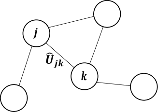
Figure 1: Harmonic oscillator graph state: each oscillator can be associated with the graph vertex, action of the unitary operator $\hat{U}_{jk}$ on the ground state of a system of $N$ non-interacting harmonic oscillators corresponds to the edge between the vertices $j$, $k$.

Let us consider an entanglement of one oscillator with coordinate $x_{1}$ with the others. In this case ${\bf x}_{1}=(x_{1})$ and ${\bf x}_{2}=(x_{2},x_{3},x_{4}...,x_{N})$. As it was shown in the previous section, the geometric measure of an entanglement of a state is determined by the maximal eigenvalue of equation (15). Taking into account (16) in the case when the state is defined as (18) one has

$$K({x}_{1},x^{\prime}_{1})=\int dx_{2}dx_{3}...dx_{N}\psi^{\ast}(x_{1},x_{2},...,x_{N})\psi(x^{\prime}_{1},x_{2},...,x_{N})=$$

$$=\sqrt{\frac{\pi}{\alpha}}\exp\Big{(}-\frac{\kappa}{4\alpha}(x_{1}-x^{\prime}_{1})^{2}-\frac{\alpha}{2}(x_{1}^{2}+(x^{\prime}_{1})^{2})\Big{)}\,,$$ (20)

where

$$\kappa_{1}=\sum_{j}a_{1j}\,.$$ (21)

So, to find the geometric measure of an entanglement one has to consider the following equation

$$\sqrt{\frac{\pi}{\alpha}}\int dx^{\prime}_{1}\exp\left(-\left(\frac{\kappa_{1}}{4\alpha}+\frac{\alpha}{2}\right)(x_{1}^{2}+(x^{\prime}_{1})^{2})+\frac{\kappa_{1}}{2\alpha}x_{1}x^{\prime}_{1}\right)\phi_{1}(x^{\prime}_{1})=\lambda\phi_{1}({x}_{1}).$$ (22)

The solution of (22) reads

$$\phi_{n}(x_{1})=\sum^{n}_{i=0}C_{i}x_{1}^{i}e^{-\frac{\kappa_{1}}{2\alpha}x_{1}^{2}},$$ (23)

$$\lambda_{n}=\frac{2\alpha\kappa_{1}^{n}}{(\kappa_{1}+2\alpha^{2}+2\alpha\sqrt{\alpha^{2}+\kappa_{1}})^{n+\frac{1}{2}}},$$ (24)

with $C_{i}$ being constants. It is easy to show that the spectrum of eigenvalues $\lambda_{n}$ attains maximal value at $n=0$ leading to

$$\lambda_{\rm max}=\lambda_{0}=\frac{2\alpha}{\sqrt{\kappa_{1}+2\alpha^{2}+2\alpha\sqrt{\alpha^{2}+\kappa_{1}}}}=\frac{2}{1+\sqrt{1+\kappa_{1}/\alpha}}\,.$$ (25)

Finally, taking into account (17) one gets that the geometric measure of an entanglement of a single oscillator in interacting kicked oscillator graph state is determined as

$$E=\frac{\sqrt{1+\kappa_{1}/\alpha}-1}{\sqrt{1+\kappa_{1}/\alpha}+1}.$$ (26)

It is worth noting that $\kappa_{1}$ as given by (21) is nothing else but the degree of the vertex 1 that corresponds to the oscillator whose entanglement is being measured. Therefore, according to (26) an entanglement of a harmonic oscillator depends on the value of degree of the vertex which represents it. Note that the entanglement increases with an increase of $\kappa_{1}$. This manifests correlation of an entanglement of a harmonic oscillator with the number of edges incident to the corresponding vertex in the graph.

4 Conclusions

We propose the way to quantify the geometric measure of entanglement for continuous variable states. We show that the entanglement is related with the maximal eigenvalue of the eigenvalue equation (15).

On the basis of the proposed way to quantify entanglement (17) we have studied entanglement of graph states. We have considered the states obtained as a result of an action of the unitary operator $\hat{U}_{jk}=\exp(ia_{jk}x_{j}x_{k})$ on the ground state of a system of $N$ noninteracting harmonic oscillators. We have obtained that the entanglement of a single harmonic oscillator depends on the value of degree of the vertex which represents it. So, there is a correlation of the entanglement of a harmonic oscillator with number of edges incident to the corresponding vertex in the graph.

References

- [1] A. Einstein, B. Podolsky, and N. Rosen, Phys. Rev. 47, 777 (1935).
- [2] E. Schrdinger, Naturwiss. 23, 807 (1935); 23, 823 (1935); 23, 844 (1935).
- [3] R. Horodecki, P. Horodecki, M. Horodecki, K. Horodecki, Rev. Mod. Phys. 81, 865 (2009).
- [4] A. Shimony, Ann. N.Y. Acad. Sci. 755, 675 (1995).
- [5] B. K. Behera, S. Seth, A. Das, P. K. Panigrahi, Quantum Information Processing 18, 108 (2019).
- [6] A. J. Scott, Phys. Rev. A 69, 052330 (2004).
- [7] P. Horodecki, A. Ekert Phys. Rev. Lett. 89, 127902 (2002).
- [8] M. B. Plenio, S. Virmani, Quantum Inf. Comp. 7, 1 (2007).
- [9] J. Torrico, M. Rojas, S. M. de Souza, et al, EPL (Europhysics Letters), 108, 50007 (2014).
- [10] Yu-Bo Sheng, Lan Zhou, EPL (Europhysics Letters) 109, 40009 (2015).
- [11] A. M. Frydryszak, M. I. Samar, V. M. Tkachuk, Eur. Phys. J. D 71, 233 (2017).
- [12] A. R. Kuzmak, V. M. Tkachuk, Phys. Lett. A 384, 126579 (2020).
- [13] Kh. P. Gnatenko, V. M. Tkachuk, Phys. Lett. A 396, 127248 (2021).
- [14] A. R. Kuzmak, V. M. Tkachuk, Eur. Phys. J. Plus 136, 564 (2021).
- [15] Kh. P. Gnatenko, N. A. Susulovska, EPL (Europhysics Letters) (2021) .
- [16] Yuanhao Wang, Ying Li, Zhang-qi Yin, Bei Zeng, npj Quant. Inf. 4, 46 (2018).
- [17] G. J. Mooney, Ch. D. Hill, L. C. L. Hollenberg, Sci. Rep. 9, 13465 (2019).
- [18] C. H. Bennett, G. Brassard, C. Crepeau, R. Jozsa, A. Peres, W. K. Wootters, Phys. Rev. Lett. 70, 1895 (1993).
- [19] D. Bouwmeester, J.-W. Pan, K. Mattle, M. Eibl, H. Weinfurter, A. Zeilinger, Nature 390, 575 (1997).
- [20] A. K. Ekert, Phys. Rev. Lett., 67, 661 (1991).
- [21] R. Raussendorf, H. J. Briegel, Phys. Rev. Lett. 86, 5188 (2001).
- [22] S. Lloyd, Science 273, 1073 (1996).
- [23] I. Buluta, F. Nori, Science 326, 108 (2009).
- [24] Shaoping Shi, Long Tian, Yajun Wang et al, Phys. Rev. Lett. 125, 070502 (2020).
- [25] D. Llewellyn, Yu. Ding, I. I. Faruque et al, Nature Physics 16, 148 (2020).
- [26] Ni-Ni Huang, Wei-Hao Huang, Che-Ming Li, Scientific Reports 10, 3093 (2020).
- [27] Juan Yin, Yu-Huai Li, Sheng-Kai Liao et al, Nature 582, 501 (2020).
- [28] T. Jennewein, Ch. Simon, G. Weihs et al, Phys. Rev. Lett. 84, 4729 (2000).
- [29] A. Karlsson, M. Bourennane, Phys. Rev. A 58, 4394 (1998).
- [30] D. N. Makarov, Phys. Rev. E 97, 042203 (2018).
- [31] M. B. Plenio, J. Hartley, J. Eisert New Journal of Physics 6, 36 (2004).
- [32] T. C. Wei, P. M. Goldbart, Phys. Rev. A 68, 042307 (2003).
- [33] J. Martin, O. Giraud, P. A. Braun, D. Braun, T. Bastin, Phys. Rev. A 81, 062347 (2010).
- [34] S. Tamaryan, A. Sudbery, L. Tamaryan, Phys. Rev. A 81, 052319 (2010).
- [35] D. Markham, A. Miyake, Sh. Virmani, New J. Phys. 9, 194 (2007).
- [36] L. Tamaryan, D. Park, S. Tamaryan, Phys. Rev. A 77, 022325 (2008).
- [37] Ali Saif M. Hassan, Pramond S. Jong, Phys. Rev. A 77, 062334 (2008).
- [38] M. Hayashi, D. Markham, M. Murao, M. Owari, Sh. Virmani, J. Math. Phys. 50, 122104 (2009).
- [39] L. Tamaryan, Z. Ohanyan, S. Tamaryan, Phys. Rev. A 82 022309 (2010).
- [40] L. Chen, A. Xu, H. Zhu, Phys. Rev. A 82 032301 (2010).
- [41] A. Streltsov, H. Kampermann, D. Bruss, Phys. Rev. A 84, 022323 (2011).
- [42] O. Pfister, J. Phys. B: At. Mol. Opt. Phys. 53, 012001 (2020).
- [43] M. Gu, Ch. Weedbrook, N. C. Menicucci, T. C. Ralph, P. van Loock, Phys. Rev. A 79, 062318 (2009).
- [44] S. A. Gardiner, J. I. Cirac, P. Zoller, Phys. Rev. Lett. 79, 4790 (1997); Erratum Phys. Rev. Lett. 80, 2968 (1998).