CertiStr: A Certified String Solver

Abstract.

Theories over strings are among the most heavily researched logical theories in the SMT community in the past decade, owing to the error-prone nature of string manipulations, which often leads to security vulnerabilities (e.g. cross-site scripting and code injection). The majority of the existing decision procedures and solvers for these theories are themselves intricate; they are complicated algorithmically, and also have to deal with a very rich vocabulary of operations. This has led to a plethora of bugs in implementation, which have for instance been discovered through fuzzing.

In this paper, we present CertiStr, a certified implementation of a string constraint solver for the theory of strings with concatenation and regular constraints. CertiStr aims to solve string constraints using a forward-propagation algorithm based on symbolic representations of regular constraints as symbolic automata, which returns three results: sat, unsat, and unknown, and is guaranteed to terminate for the string constraints whose concatenation dependencies are acyclic. The implementation has been developed and proven correct in Isabelle/HOL, through which an effective solver in OCaml was generated. We demonstrate the effectiveness and efficiency of CertiStr against the standard Kaluza benchmark, in which 80.4% tests are in the string constraint fragment of CertiStr. Of these 80.4% tests, CertiStr can solve 83.5% (i.e. CertiStr returns sat or unsat) within 60s.

1. Introduction

Strings are among the most fundamental and commonly used data types in virtually all modern programming languages, especially with the rapidly growing popularity of dynamic languages, including JavaScript and Python. Programs written in such languages often implement security-critical infrastructure, for instance web applications, and they tend to process data and code in string representation by applying built-in string-manipulating functions; for instance, to split, concatenate, encode/decode, match, or replace parts of a string. Functions of this kind are complex to reason about and can easily lead to programming mistakes. In some cases, such mistakes can have serious consequences, e.g., in the case of web applications, cross-site scripting (XSS) attacks can be used by a malicious user to attack both the web server or the browsers of other users.

One promising research direction, which has been intensively pursued in the SMT community in the past ten years, is the development of SMT solvers for theories of strings (dubbed string solvers) including Kaluza (Saxena et al., 2010), CVC4 (Liang et al., 2014), Z3 (de Moura and Bjørner, 2008), Z3-str3 (Berzish et al., 2017), Z3-Trau (Bui and contributors, 2019), S3P (Trinh et al., 2016), OSTRICH (Chen et al., 2019), SLOTH (Holík et al., 2018), and Norn (Abdulla et al., 2014), to name only a few. Such solvers are highly optimized and find application, among others, in bounded model checkers and symbolic execution tools (Cordeiro et al., 2018; Noller et al., 2019), but also in tools tailored to verification of the security properties (Backes et al., 2018).

It has long been observed that constraint solvers are extremely complicated procedures, and that implementations are prone to bugs. Defects that affect soundness or completeness are routinely found even in well-maintained state-of-the-art tools, both in real-world applications and through techniques like fuzzing (Bugariu and Müller, 2020; Blotsky et al., 2018; Mansur et al., 2020). String solvers are particularly troublesome in this context, since, unlike other SMT theories, the theory of strings requires a multitude of operations including concatenation, regular constraints, string replacement, length constraints, and many others. This inherent intricacy is also reflected in the recently developed SMT-LIB standard for strings (http://smtlib.cs.uiowa.edu/theories-UnicodeStrings.shtml). Many of the string solvers that arose in the past decade relied on inevitably intricate decision procedures, which resulted in subtle bugs in implementations themselves even among the mainstream string solvers (e.g. see (Bugariu and Müller, 2020; Mansur et al., 2020)). This implies the unfortunate fact that one cannot blindly trust the answer provided by string solvers.

Contributions.

In this paper, we present CertiStr, the first certified implementation of a string solver for the standard theory of strings with concatenation and regular constraints (a.k.a. word equations with regular constraints (Makanin, 1977; Gutiérrez, 1998; Jez, 2016; Diekert, 2002)). CertiStr aims to solve string constraints by means of the so-called forward-propagation algorithm, which relies on a simple idea of propagating regular constraints in a forward direction in order to derive contradiction, or prove the absence thereof (see Section 2 for an example). Similar ideas are already present in abstract interpretation of string-manipulating programs (e.g. see (Yu et al., 2014; Minamide, 2005; Wang et al., 2016)), but not yet at the level of string solvers, i.e., which operate on string constraints. We have proven in Isabelle/HOL (Nipkow et al., 2002) some crucial properties of the forward-propagation algorithm and more specifically with respect to our implementation CertiStr: (i) [TERMINATION]: the algorithm terminates on string constraints without cyclic concatenation dependencies, (ii) [SOUNDNESS]: CertiStr  is sound for unsatisfiable results (if forward-propagation detects inconsistencies in a constraint, then the constraint is indeed unsatisfiable), and (iii) [COMPLETENESS]: CertiStr  is complete for constraints satisfying the tree property (i.e., in which on the right-hand side of each equation every variable appears at most once). Here completeness amounts to the fact that, if forward-propagation does not detect inconsistencies for a constraint satisfying the tree property, then the constraint is indeed satisfiable. For the constraints that do not satisfy the tree property and CertiStr cannot decide them as unsatisfiable, CertiStr returns unknown.

In order to facilitate the propagation of regular constraints, we also implement a certified library for Symbolic Non-deterministic Finite Automata (s-NFA), which contains various automata operations, such as the concatenation and product of two s-NFAs, the language emptiness checking for s-NFAs, among others. s-NFAs — as introduced by Veanes et al. (Veanes et al., 2012) (see (D’Antoni and Veanes, 2021) for more details) — are different from classic Non-deterministic Finite Automata (NFA) by allowing transition labels to be a set of characters in the (potentially infinite) alphabet, represented by an element of a boolean algebra (e.g. the interval algebra or the BDD algebra), instead of a single character. s-NFAs are especially crucial for an efficient implementation of automata-based string solving algorithms and many string processing algorithms (Klarlund et al., 2002; Veanes et al., 2012; D’Antoni and Veanes, 2021; Chen et al., 2019; Abdulla et al., 2014), for which reason our certified implementation of an s-NFA library is of independent interests.

Last but not least, we have automatically generated a verified implementation CertiStr in Isabelle/HOL, which we have extensively evaluated against the standard string solving benchmark from Kaluza (Saxena et al., 2010) with around 38000 string constraints. For the first time, we demonstrate that the simple forward-propagation algorithm in fact performs surprisingly well even compared to other highly optimized solvers (which are not verified implementations). In particular, we show that the majority of these constraints (83.5%) are solved by CertiStr; for the rest, the tool either returns unknown, or times out. Moreover, CertiStr terminates within 60 seconds on 98% of the constraints, witnessing its efficiency.

To summarize, our contributions are:

• we developed in Isabelle/HOL the tool CertiStr, the first certified implementation of a string solver.

• we implemented the first certified symbolic automata library, which is crucial for an efficient implementation of many string processing applications (D’Antoni and Veanes, 2021).

• CertiStr was evaluated over Kaluza benchmark (Saxena et al., 2010), with around 38000 tests. In this benchmark, 83.5% of the tests can be solved with the results sat or unsat. Moreover, the solver terminates within 60 seconds on 98% of the tests, witnessing the surprising competitiveness of the simple forward-propagation algorithm against more complicated algorithms.

2. Motivating Example

We start by illustrating the decision procedure implemented by CertiStr. CertiStr uses the so-called forward-propagation algorithm for solving satisfiability of string theory with concatenation and regular membership constraints. To illustrate the algorithm, consider the formula:

(1) $$\mathit{domain} ~{}\in~{}\texttt{/[a-zA-Z.]+/}$$

(2) $$\mbox{}\wedge\makebox[34.44434pt][r]{$\mathit{dir}$, $\mathit{file}$} ~{}\in~{}\texttt{/[a-zA-Z0-9.]+/}$$

(3) $$\mbox{}\wedge\makebox[34.44434pt][r]{$\mathit{path}$} ~{}=~{}\mathit{dir}+\texttt{"/"}+\mathit{file}$$

(4) $$\mbox{}\wedge\makebox[34.44434pt][r]{$\mathit{url}$} ~{}=~{}\texttt{"http://"}+\mathit{domain}+\texttt{"/"}+\mathit{path}$$

(5) $$[\mbox{}\wedge\makebox[34.44434pt][r]{$\mathit{url}$} ~{}\in~{}\texttt{/.*<script>.*/}]$$

The formula contains string variables (domain, dir, etc.), and uses both regular membership constraints and word equations with concatenation to model the construction of a URL from individual components. Regular expressions are written using the standard PCRE syntax (https://perldoc.perl.org/perlre). Each equation should be read as an assignment of the right-hand side term to the left-hand side variable, and is processed in this direction. We initially ignore the constraint (5).

The forward-propagation algorithm propagates regular membership constraints and derives new constraints for the variable on the left-hand side of equations. In this example, the algorithm starts with equation (3) and propagates constraint (2), resulting in the new constraint

(6) $$\mathit{path}~{}\in~{}\texttt{/[a-zA-Z0-9.]+\textbackslash/[a-zA-Z0-9.]+/}$$

We can propagate this new constraint further, using equation (4) and together with constraint (1), deriving:

(7) $$\mathit{url}~{}\in~{}\texttt{/http:\textbackslash/\textbackslash/[a-zA-Z.]+}\\ \texttt{\textbackslash/[a-zA-Z0-9.]+\textbackslash/[a-zA-Z0-9.]+/}$$

At this point, no more propagations are possible. Note that forward-propagation will terminate, in general, whenever no cyclic dependencies exist between the equations, which is the fragment of formulas we consider.

Still ignoring (5), we can observe that forward-propagation has not discovered any inconsistent constraints. In order to conclude the satisfiability of the formula from this, we need a meta-result about forward-propagation: we show that forward propagation is complete for acyclic formulas in which each variable occurs at most once on the right-hand side of equations. Since this criterion holds for the formula $\eqref{eq:1}\wedge\cdots\wedge\eqref{eq:4}$, we have indeed proven that it is satisfiable.

Consider now also (5), modelling a simple form of injection attack. We can observe that this additional constraint is inconsistent with the derived constraint (7), since the intersection of the asserted regular languages is empty. Forward-propagation detects this conflict as soon as (7) has been computed: each time a new membership constraint is derived, the algorithm will check the consistency with constraints already assumed. Since we also show that forward-propagation is sound w.r.t. inconsistency, the detection of a conflict immediately implies that the formula $\eqref{eq:1}\wedge\cdots\wedge\eqref{eq:5}$ is unsatisfiable.

In summary, the forward-propagation is defined using two main inference steps: the post-image computation for word equations, and a consistency check for regular constraints. Although the example uses regular expressions, both operations can be defined more easily through a translation to finite-state automata. To obtain a verified string solver, the implementation of both operations has to be shown correct, and in addition meta-results need to be derived about the soundness and completeness of the overall algorithm.

We can also observe that classical finite-state automata, over concrete alphabets, are cumbersome even for toy examples; regular expressions often talk about character ranges that would require a large number of individual transitions. In practice, string constraints are usually formulated over the Unicode alphabet with currently $3\times 2^{16}$ characters, which necessitates symbolic character representation. In our verified implementation, we therefore use a simple form of symbolic automata (D’Antoni and Veanes, 2017) in which transitions are labelled with character intervals.

3. String Constraint Fragment

In this section, we present the string constraint fragment that CertiStr supports and its semantics of satisfiability.

Let $\Sigma$ be an alphabet and $\Sigma^{*}$ denote the set of words over $\Sigma$. Let $w_{1},w_{2}\in\Sigma^{*}$ be two words, $w_{1}w_{2}$ denotes the concatenation of the two words, i.e., $w_{2}$ is appended to the end of $w_{1}$ to get a new string. We consider the following string constraint language over $\Sigma$:

$$c::=x\in\mathcal{A}\mid x=x_{1}+x_{2}\mid c_{1}\wedge c_{2},$$

where $x$ denotes a variable ranging over $\Sigma^{*}$ and $\mathcal{A}$ denotes an NFA representing a regular language over $\Sigma$. The language accepted by $\mathcal{A}$ is denoted by $\mathcal{L}(\mathcal{A})$. The semantics of a constraint $c$ is defined in an obvious way by interpreting $x\in\mathcal{A}$ as a membership of $x$ in the language $\mathcal{L}(\mathcal{A})$, $x=x_{1}+x_{2}$ as a string equation, and $c_{1}\wedge c_{2}$ as a conjunction of $c_{1}$ and $c_{2}$. More precisely, given a function $\mu$ mapping each variable in the constraint $c$ to a string in $\Sigma^{*}$, we say that $\mu$ satisfies $c$ if: (i) $\mu(x)\in\mathcal{L}(\mathcal{A})$ for each constraint $x\in\mathcal{A}$ in $c$, and (ii) $\mu(x)=\mu(x_{1})\mu(x_{2})$ for each constraint $x=x_{1}+x_{2}$. The constraint $c$ is satisfiable if one such solution $\mu$ for $c$ exists.

Our string constraint language is as general as word equations with regular constraints (Makanin, 1977; Gutiérrez, 1998; Jez, 2016; Diekert, 2002), which forms the basis of the recently published Unicode string constraint language in SMT-LIB 2.6, and already makes up the bulk of existing string constraint benchmarks. Notice that our restriction to string equation of the form $x=x_{1}+x_{2}$ is not a real restriction since general string constraints can be obtained by means of desugaring. For instance, the concatenation of more than two variables, like $x=x_{1}+x_{2}+x_{3}$ can be desugared as two concatenation constraints: $(1)~{}x^{\prime}=x_{1}+x_{2};x=x^{\prime}+x3$. Moreover, a subset of string constraints with length functions (called monadic length) can also be translated into this fragment with regular constraints. For instance, $|x|\leq 6$, where $|x|$ denotes the length of the word of $x$, can be translated to a regular membership constraint as $x\in\mathcal{\mathcal{A}}$, where $\mathcal{\mathcal{A}}$ is an NFA that accepts any word whose length is at most $6$. Recent experimental evidence shows that a substantial portion of length constraints that appear in practice are essentially monadic (Hague et al., 2020). There are also some string constraints using disjunction ($\vee$). For instance, $c_{1}\vee c_{2}$, where $c_{1}$ and $c_{2}$ are string constraints in our fragment. This also can be solved with CertiStr by first solving $c_{1}$ and $c_{2}$ separately, and then checking whether one of them is satisfiable.

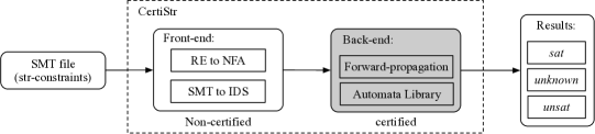
Figure 1. The framework of the certified string solver

Figure 1 shows the framework of CertiStr. The input of the solver is an SMT file with string constraints. The tool has two parts: (1) the front-end (non-certified) and (2) the back-end (certified). The front-end parses the SMT file, which will first translate all Regular Expressions (RE) to NFAs and desugar some string constraints that are not in the fragment, and then translate the string constraints to the Intermediate Data Structures (IDS), which are the inputs of the back-end. The IDS contains three parts: (1) a set $S$ of variables that are used in the string constraints, (2) a concatenation constraint map $\mathit{Concat}$, which maps variables in $S$ to the set of their concatenation constraints, and (3) a regular constraint map $\mathit{Reg}$, which maps each variable in $S$ to its regular membership constraints.

The back-end contains two parts: (1) the Automata Library, which contains a collection of automata operations, such as the product and concatenation of two NFAs, and (2) a forward-propagation to check whether the string constraints are satisfiable. The results of the certified string solver can be (1) sat the string constraint is satisfiable, (2) unsat the string constraint is unsatisfiable, and (3) unknown the solver cannot decide whether the string constraint is satisfiable or not. Note that, unknown does not mean that CertiStr is non-terminating. It means the results after executing the forward-propagation for string constraints are not sufficient to decide their satisfiability.

4. Forward-propagation of String Constraints

In this section, we present the algorithm of the forward-propagation and the properties proven for it.

4.1. The Algorithm of Forward-propagation

We use the following example of string constraints to illustrate our forward-propagation analysis.

Example 4.1.

$x_{1}\in\mathcal{A}_{1}\wedge x_{2}\in\mathcal{A}_{2}\wedge x_{3}\in\mathcal{A}_{3}\wedge x_{5}=x_{3}+x_{4}\wedge x_{3}=x_{1}+x_{2}$.

Figure 2. Dependence graph of variables in Example 4.1

Example 4.1 contains five variables “$x_{1},x_{2},x_{3},x_{4},x_{5}$” and two concatenation constraints “$x_{5}=x_{3}+x_{4}\wedge x_{3}=x_{1}+x_{2}$”. We can view these concatenation constraints as a dependence graph shown in Figure 2. For a concatenation constraint $x_{k}=x_{i}+x_{j}$, it yields two dependence relations: $x_{k}\mapsto x_{i}$ and $x_{k}\mapsto x_{j}$ ($a\mapsto b$ denotes $a$ depends on $b$). This means that before propagating the concatenation of the regular constraints of $x_{i}$ and $x_{j}$ to $x_{k}$, we need to first compute the propagation to $x_{i}$ and $x_{j}$. Let the initial regular constraint of $x_{k}$ be $\mathcal{A}_{k}$. Let the regular constraints of $x_{i}$ and $x_{j}$ be $\mathcal{A}_{i}$ and $\mathcal{A}_{j}$, respectively. The new regular constraint of $x_{k}$ after the propagation can be refined to an automaton, whose language is $\mathcal{L}(\mathcal{A}_{k})\cap(\mathcal{L}(\mathcal{A}_{i})+\mathcal{L}(\mathcal{A}_{j}))$, where $\mathcal{L}_{1}+\mathcal{L}_{2}\triangleq\{w_{1}w_{2}\mid w_{1}\in\mathcal{L}_{1}\land w_{2}\in\mathcal{L}_{2}\}$. Here, the term “refine” means narrowing the regular constraint of a variable by propagating the concatenation constraints.

The forward-propagation repeats the following computation until all variables are refined:

• detect a set of variables such that for each variable in the set, all its dependence variables have already been refined.

• refine the regular constraints of the variables detected in the last step with respect to their concatenation constraints.

We illustrate the idea of the forward-propagation with Example 4.1. The first iteration of the forward-propagation will detect the set of variables $\{x_{1},x_{2},x_{4}\}$ since they have no dependence variables and we do not need to refine their regular constraints. The second iteration of the forward-propagation will detect the set of variables: $\{x_{3}\}$, as $x_{3}$ only depends on the variables in $\{x_{1},x_{2},x_{4}\}$. Its regular constraint will be refined to an automaton, whose language is $\mathcal{L}(\mathcal{A}_{3})\cap(\mathcal{L}(\mathcal{A}_{1})+\mathcal{L}(\mathcal{A}_{2}))$ after the propagation for the constraint $x_{3}=x_{1}+x_{2}$. Assume this new regular constraint as $\mathcal{A}_{3}^{\prime}$. The third iteration detects the variable $x_{5}$, whose regular constraint will be refined to an automaton, whose language is $\Sigma^{*}\cap(\mathcal{L}(\mathcal{A}_{3}^{\prime})+\Sigma^{*})$. Note that we do not specify the initial regular constraints of $x_{4}$ and $x_{5}$ in the string constraint and therefore their initial regular constraints are $\Sigma^{*}$ by default.

Algorithm 1 shows the forward-propagation algorithm. It contains three procedures: $\mathbf{Forward\_Prop}$, $\mathbf{Ready\_Set}$, and $\mathbf{Var\_Lang}$. The procedure $\mathbf{Forward\_Prop}$ is the entry point of the algorithm and has three parameters: (1) $S$ is the set of variables used in the string constraints, for instance, in Example 4.1, there are five variables: $S=\{x_{1},x_{2},x_{3},x_{4},x_{5}\}$; (2) $\mathit{Concat}:S\rightharpoonup 2^{(S\times S)}$ is a partial map which maps a variable $x$ to a set of pairs of variables. For each pair $(x_{1},x_{2})$ in the set, there is a concatenation constraint: $x=x_{1}+x_{2}$; (3) $\mathit{Reg}:S\rightarrow\mathcal{N}$ is a map from variables to automata. These automata denote the variables’ initial regular constraints. Here $\mathcal{N}$ denotes the set of NFAs.

Algorithm 1 The algorithm of forward-propagation

1:procedure $\mathbf{Forward\_Prop}$($S,\mathit{Concat},\mathit{Reg}$)  

2:     $R\leftarrow\emptyset$

3:     while $S\neq\emptyset$ do

4:         $C$ $\leftarrow$ $\mathbf{Ready\_Set}$($S,\mathit{Concat},R$)

5:         $\mathit{Reg}$ $\leftarrow$ $\mathbf{Var\_Lang}$($C,\mathit{Concat},\mathit{Reg}$)

6:         $S$ $\leftarrow$ $S~{}-~{}C$; $R$ $\leftarrow$ $R~{}\cup~{}C$

7:     end while

8:     return $\mathit{Reg}$

9:end procedure

10:procedure $\mathbf{Var\_Lang}$($C,\mathit{Concat},\mathit{Reg}$)

11:     for each $v\in C$ do

12:         $\mathcal{A}$ $\leftarrow$ $(\mathit{Reg}~{}v)$

13:         for each $(v_{1},v_{2})\in(\mathit{Concat}~{}v)$ do

14:              $\mathcal{A^{\prime}}\leftarrow\mathbf{NFA\_concat}~{}(\mathit{Reg}~{}v_{1})~{}(\mathit{Reg}~{}v_{2})$

15:              $\mathcal{A}$ $\leftarrow$ $\mathbf{NFA\_product}~{}\mathcal{A}~{}~{}\mathcal{A}^{\prime}$

16:         end for

17:         $\mathit{Reg}~{}\leftarrow~{}\mathit{Reg}~{}[v\mapsto\mathcal{A}]$

18:     end for

19:     return $\mathit{Reg}$

20:end procedure

22:procedure $\mathbf{Ready\_Set}$($S,\mathit{Concat},R$)

23:     $C$ $\leftarrow$ $\emptyset$

24:     for each $v\in S$ do

25:         $D$ $\leftarrow$ $\emptyset$

26:         for each $(v_{1},v_{2})\in(\mathit{Concat}~{}v)$ do

27:              $D$ $\leftarrow$ $D~{}\cup~{}\{v_{1},v_{2}\}$

28:         end for

29:         if $D~{}\subseteq R$ then

30:              $C~{}\leftarrow~{}C~{}\cup~{}\{v\}$

31:         end if

32:     end for

33:     return $C$

34:end procedure

In the while loop of the procedure $\mathbf{Forward\_Prop}$, the computation iteratively refines the regular constraints of variables by propagating the regular constraints of variables on the right hand side of the concatenation constraints. The first step in the loop computes the set $C$ of variables whose dependence variables are all in the set $R$ (computed by the procedure $\mathbf{Ready\_Set}$). $R$ is initialized empty and it denotes the set of variables that have already been refined by the previous loops. The second step in the loop updates the regular constraints of the variables in $C$ stored in $\mathit{Reg}$ by propagating the concatenation constraints in $\mathit{Concat}$ (computed by $\mathbf{Var\_Lang}$).

At the end of the loop body, the set $S$ is updated by removing the variables in $C$ as they have already been refined and these removed variables are added to the set $R$, i.e., they have already been refined.

The procedure $\mathbf{Ready\_Set}$ computes the set of variables that are only dependent on the variables in $R$. For each variable $v$, it stores all its dependence variables in $D$ and then checks whether $D$ is a subset of $R$. If $D$ is a subset of $R$ then $v$ is moved to $C$ as all its dependence variables have been refined.

The procedure $\mathbf{Var\_Lang}$ refines the regular constraints of variables in $C$. In the inner loop of $\mathbf{Var\_Lang}$, it traverses all concatenation constraints $v=v_{1}+v_{2}$ and refines the regular constraint of $v$ by propagating the concatenation of the regular constraints of $v_{1}$ and $v_{2}$. $\mathit{Reg}~{}[v\mapsto\mathcal{A}]$ means updating the regular constraint of $v$ in $\mathit{Reg}$ to $\mathcal{A}$. The functions $\mathbf{NFA\_concat}$ and $\mathbf{NFA\_product}$ denote constructing the concatenation and product of two NFAs, respectively. These two functions will be introduced in Section 5.

Assume a string constraint is stored in $S$, $\mathit{Concat}$ and $\mathit{Reg}$, then after calling “$\mathbf{Forward\_Prop}(S,~{}\mathit{Concat},~{}\mathit{Reg})"$, we will get a new $\mathit{Reg}^{\prime}$ such that for each variable $v$, $(\mathit{Reg}^{\prime}~{}v)$ stores the refined regular constraint of $v$, which is an NFA. We have two cases to decide whether the string constraint is satisfiable or not:

• If there exists a variable $v$ such that the language of $(\mathit{Reg}^{\prime}~{}v)$ is empty then the string constraint is unsatisfiable, because the refined regular constraint of $v$ is the empty language.

• If for all variables $v$ such that the language of $(\mathit{Reg}^{\prime}~{}v)$ is not empty then unfortunately we cannot decide whether the string constraint is satisfiable or not. Consider the string constraint: “(1) $y=x+x\wedge(2)~{}y\in\{ab\}\wedge(3)~{}x\in\{a,b\}$”, where $ab$, $a$, and $b$ are words, the refined regular constraints of $x$ and $y$ are both not empty. But this string constraint is not satisfiable as constraints (1) and (2) require $x$ to have two different values. We will introduce a property, called tree property later, such that if the string constraint satisfies the tree property then it is satisfiable, otherwise CertiStr returns unknown.

4.2. Theorems for Forward-propagation

Now we introduce the key theorem proven for the algorithm. Firstly we present the definitions of well-formed inputs ($\mathbf{wf}$ in Figure 3) and the acyclic property ($\mathbf{acyclic}$ in Figure 3) for concatenation constraints, which are the premises of the correctness theorem.

The $\mathbf{wf}$ predicate requires that all variables appearing in the domain and codomain of $\mathit{Concat}$ should be in the set $S$, and the domain of $\mathit{Reg}$ should be the set $S$, i.e., all variables should have their initial regular constraints. $S$ should be finite. Now we consider the definition of $\mathbf{acyclic}$, which checks whether the dependence graphs of concatenation constraints are acyclic. $\mathbf{Forward\_Prop}$ cannot solve string constraints that are not acyclic. For instance, the string constraint “$x=y_{1}+y_{2}\wedge y_{1}=z_{1}+x$” does not satisfy the acyclic property, as $x\mapsto y_{1}\mapsto x$.

⬇

definition $\mathbf{wf}$ where

$\mathbf{wf}$ $S$ $\mathit{Concat}$ $\mathit{Reg}$ =

$(dom$ $\mathit{Concat}$ $\subseteq$ $S$)$\land$($dom$ $\mathit{Reg}$ = $S$)$\land$

$(\forall$ $v$ $v_{1}$ $v_{2}.$ $v\in$$(dom$ $\mathit{Concat}$$)\land(v_{1},v_{2})\in(\mathit{Concat}$ $v)$

$\longrightarrow v_{1}\in S$ $\land$ $v_{2}\in S)$ $\land$ finite $S$

definition $\mathbf{acyclic}$ where

$\mathbf{acyclic}$ $S$ $\mathit{Concat}$ $l$ = $S=\bigcup(\mathbf{set}$ $l)\land((l=[])$

$\lor(l=s\#l^{\prime}\longrightarrow(s\cap(\bigcup(\mathbf{set}$ $l^{\prime}))=\emptyset)$ $\land$

$(\forall v_{1}$ $v_{2}$ $v.$ $v\in s\land(v_{1},v_{2})\in(\mathit{Concat}$ $v)\longrightarrow$

$\{v_{1},v_{2}\}\subseteq\bigcup(\mathbf{set}$ $l^{\prime}))\land$$(\mathbf{acyclic}$ $(S-s)$ $\mathit{Concat}$ $l^{\prime})))$

Figure 3. The definitions of $\mathbf{wf}$ and $\mathbf{acyclic}$

In order to specify the acyclic property, we arrange the set $S$ of variables to a list in which elements are disjoint sets of variables in $S$ and the list characterizes the dependence levels among variables. For instance, in Example 4.1, there are $5$ variables and they can be organized in a list: $[\{v_{5}\},\{v_{3}\},\{v_{1},v_{2},$ $v_{4}\}]$. Indeed, the list characterizes the dependence levels among variables. For instance, the variable $v_{5}$ only depends on the variables in $\{v_{3}\}$ and $\{v_{1},v_{2},v_{4}\}$ and $v_{3}$ only depends on the variables in $\{v_{1},v_{2},v_{4}\}$ but not $\{v_{5}\}$. The variables in $\{v_{1},v_{2},v_{4}\}$ do not depend on any variables. If $\mathit{Concat}$ does not satisfies the acyclic property then we cannot arrange all variables in such a list, as all variables in a cycle always depend on another variable in the cycle.

The predicate $\mathbf{acyclic}$ contains two parts. (1) $S=\bigcup(\mathbf{set}~{}l)$, which means the elements in $S$ and $l$ should be exactly the same. “$\mathbf{set}~{}l$” translates the list $l$ to a set of elements in $l$ and “$\bigcup(\mathbf{set}~{}l)=\{x\mid\exists y.y\in\mathbf{set}~{}l\land x\in y\}$”. (2) Part 2 further has two cases. The first case is “$l=[]$”, i.e., empty list. In this case, the predicate is obviously true. The second case is “$l=s\#l^{\prime}$”, i.e., it has at least one element. $s$ is the first element and $l^{\prime}$ is the tail. In this case, firstly, it requires the elements in $s$ to be disjoint with the elements in the sets of the tail $l^{\prime}$ (checked by $s\cap(\bigcup(\mathbf{set}~{}l^{\prime}))=\emptyset$). Secondly, let $v$ be a variable in $s$, for any two variables $v_{1}$ and $v_{2}$ that $v$ depends on, $v_{1}$ and $v_{2}$ can only be in the sets of the tail $l^{\prime}$. Thirdly, $\mathbf{acyclic}~{}(S-s)~{}\mathit{Concat}~{}l^{\prime}$ checks whether the remaining elements in $S-s$ are still acyclic w.r.t. $\mathit{Concat}$ and $l^{\prime}$. In order to check whether the variables in $S$ are acyclic w.r.t. $\mathit{Concat}$, we can specify it as “$\exists l.~{}\mathbf{acyclic}~{}S~{}\mathit{Concat}~{}l$”.

Now we are ready to introduce our correctness theorem (Theorem 4.2). The keyword fixes in Isabelle is used to define universally quantified variables. The keyword assumes is used to specify assumptions of the theorem and the keyword shows is used to specify the conclusion of the theorem. The shows part is of the form ”$M\leq\mathbf{SPEC}~{}(\lambda~{}Reg^{\prime}.~{}\Phi)$”, which means the algorithm $M$ is correct with respect to the specification $\Phi$. More precisely, the result of applying the predicate $(\lambda~{}Reg^{\prime}.~{}\Phi)$ to the output of $M$ should be true. “$\mathbf{NFA\_accept}~{}w~{}\mathcal{A}$” checks whether $w$ is accepted by $\mathcal{A}$, which will be introduced in Section 5. The symbol “$@$” is the list concatenation operation in Isabelle. We use a list of elements in $\Sigma$ to represent a word.

Theorem 4.2 (Correctness of $\mathbf{Forward\_Prop}$).

fixes	$S$ $\mathit{Concat}$ $\mathit{Reg}$
assumes	1. $\mathbf{wf}~{}S~{}\mathit{Concat}~{}\mathit{Reg}$
	2. $(\exists l.~{}$ $\mathbf{acyclic}~{}S~{}\mathit{Concat}~{}l)$
shows	$\text{$\mathbf{Forward\_Prop}$}(S,\mathit{Concat},\mathit{Reg})\leq$ $\mathbf{SPEC}(\lambda\mathit{Reg^{\prime}}.$
	$~{}(\forall v~{}w.~{}\mathbf{NFA\_accept}~{}w~{}(\mathit{Reg}^{\prime}~{}v)\longleftrightarrow$
	$\quad(\mathbf{NFA\_accept}~{}w~{}(\mathit{Reg}~{}v)~{}\land$
	$\quad\quad(\forall v_{1}~{}v_{2}.~{}(v_{1},v_{2})\in(\mathit{Concat}~{}v)\longrightarrow$
	$\quad\quad(\exists w_{1}~{}w_{2}.~{}w=w_{1}@w_{2}~{}\land~{}$
	$\quad\quad\mathbf{NFA\_accept}~{}w_{1}~{}(\mathit{Reg}^{\prime}~{}v_{1})\land$
	$\quad\quad\mathbf{NFA\_accept}~{}w_{2}~{}(\mathit{Reg}^{\prime}~{}v_{2}))))))$

Theorem 4.2 shows that if $S,\mathit{Concat},\mathit{Reg}$ are well-formed and acyclic then after calling $\mathbf{Forward\_Prop}(S,\mathit{Concat},\mathit{Reg})$ we can get $\mathit{Reg}^{\prime}$, which satisfies: any $w$ is accepted by the automaton $(\mathit{Reg}^{\prime}~{}v)$ if and only if

1. $w$ is accepted by the original regular constraint of $v$, i.e., $(\mathit{Reg}~{}v)$, and

2. for all variables $v_{1}$ and $v_{2}$, $(v_{1},v_{2})\in\mathit{Concat}~{}v$ implies there exist $w_{1},w_{2}$ such that $w=w_{1}@w_{2}$ and $w_{i},$ for $i=1,2$, is accepted by the regular constraint $(\mathit{Reg}^{\prime}~{}v_{i})$.

That is, in the new $\mathit{Reg}^{\prime}$, the concatenation constraints are used to refine the corresponding variables.

Moreover, in Isabelle, Theorem 4.2 also requires us to prove the termination of Algorithm 1. The termination is proven by showing that in the procedure $\mathbf{Forward\_Prop}$, the number of variables in $S$ decreases progressively for each iteration. Since $S$ is finite, the algorithm must terminate.

Even though Theorem 4.2 is the key of the correctness of the forward-propagation, it does not give us an intuition with respect to the satisfiability semantics of string constraints introduced in Section 3. In the following, we will show that our forward-propagation is sound w.r.t. unsat results.

⬇

definition $\mathbf{sat\_str}$ where

$\mathbf{sat\_str}$ $S$ $\mathit{Concat}$ $\mathit{Reg}$ $\mu=$

$(\forall v\in S.$ $(\mu$ $v)\in\mathcal{L}(\mathit{Reg}$ $v))\land$

$(\forall v~{}v_{1}~{}v_{2}.~{}v\in S\land(v_{1},v_{2})\in(\mathit{Concat}$ $v)\longrightarrow$

$(\mu$ $v)=(\mu$ $v_{1})@(\mu$ $v_{2}))$

⬇

definition $\mathbf{tree}$ where

$\mathbf{tree}~{}\mathit{Concat}$ =

$(\forall v~{}v_{1}~{}v_{2}.~{}(v_{1},v_{2})\in\mathit{Concat}~{}v~{}\longrightarrow v_{1}\neq v_{2})~{}\land$

$(\forall v~{}v_{1}~{}v_{2}~{}v_{3}~{}v_{4}.~{}(v_{1},v_{2})\neq(v_{3},v_{4})~{}\land$

$(v_{1},v_{2})\in\mathit{Concat}~{}v\land(v_{3},v_{4})\in\mathit{Concat}~{}v$

$\longrightarrow\{v_{1},v_{2}\}\cap\{v_{3},v_{4}\}=\emptyset)~{}\land$

$(\forall v$ $v^{\prime}$ $v_{1}$ $v_{2}$ $v_{3}$ $v_{4}.$ $v\neq v^{\prime}\land(v_{1},v_{2})\in\mathit{Concat}$ $v$

$\land(v_{3},v_{4})\in\mathit{Concat}$ $v^{\prime}\longrightarrow\{v_{1},v_{2}\}\cap\{v_{3},v_{4}\}=\emptyset)$

Figure 4. The definitions of $\mathbf{sat\_str}$ and $\mathbf{tree}$

Firstly we need to formalize the semantics of sat and unsat for string constraints. Let $\mu$ be an assignment, which is a map $S\rightarrow\Sigma^{*}$ from variables in $S$ to words. We define the predicate $\mathbf{sat\_str}$ in Figure 4 for the semantics of the satisfiability of string constraints.

The predicate $\mathbf{sat\_str}$ contains two parts: (1) the assignment $\mu$ should respect all regular constraints and (2) the assignment $\mu$ should respect all concatenation constraints.

Theorem 4.3 shows that after executing $\mathbf{Forward\_Prop}$, we get a new map $\mathit{Reg}^{\prime}$. If there exists a variable $v$, such that $\mathcal{L}(\mathit{Reg}^{\prime}~{}v)=\emptyset$, i.e., the language of the refined regular constraint of $v$ is the empty set, then there is no assignment $\mu$ that makes the predicate “$\mathbf{sat\_str}~{}S~{}\mathit{Concat}~{}\mathit{Reg}~{}\mu$” true.

Theorem 4.3 (Soundness for unsat results).

fixes	$S$ $\mathit{Concat}$ $\mathit{Reg}$
assumes	1. $\mathbf{wf}~{}S~{}\mathit{Concat}~{}\mathit{Reg}$
	2. $(\exists l.~{}$ $\mathbf{acyclic}~{}S~{}\mathit{Concat}~{}l)$
shows	$\text{$\mathbf{Forward\_Prop}$}(S,\mathit{Concat},\mathit{Reg})\leq\mathbf{SPEC}(\lambda\mathit{Reg}^{\prime}.$
	$((\exists v.~{}\mathcal{L}(\mathit{Reg}^{\prime}~{}v)=\emptyset)\longrightarrow$
	$(\forall\mu.~{}\neg~{}\mathbf{sat\_str}~{}S~{}\mathit{Concat}~{}\mathit{Reg}~{}\mu)))$

Unfortunately, the theorem holds only for unsat results. As we already analyzed before, the case $\forall v.~{}\mathcal{L}(\mathit{Reg}^{\prime}~{}v)\neq\emptyset$ cannot make us conclude that the string constraint is satisfiable.

In this paper, we characterize a subset of the string constraints, using a property such that the forward-propagation’s satisfiable results are also sound. We call it the tree property. The intuition behind the tree property is that the dependence graph of a string constraint should constitute a tree or forest. The example $y=x+x$ does not satisfy the tree property, because $y$ has two edges pointing to a same node $x$ in the dependence graph. In other words, the node $x$ has indegree 2. But a tree requires that each node has at most indegree 1. As the map $\mathit{Concat}$ stores the dependence graphs of string constraints, we only need to check $\mathit{Concat}$ for the tree property. The predicate $\mathbf{tree}$ is defined in Figure 4.

This definition has three cases separated by the conjunction operator: (1) the first case requires that for any concatenation constraint $v=v_{1}+v_{2}$, we have $v_{1}\neq v_{2}$. (2) The second case requires that for any variable $v$ with two concatenations $v=v_{1}+v_{2}$ and $v=v_{3}+v_{4}$, $\{v_{1},v_{2}\}$ and $\{v_{3},v_{4}\}$ are disjoint. (3) The third case requires that for any two different variables $v$ and $v^{\prime}$ with the concatenation constraints $v=v_{1}+v_{2}$ and $v^{\prime}=v_{3}+v_{4}$, $\{v_{1},v_{2}\}$ and $\{v_{3},v_{4}\}$ are disjoint.

With this definition we have the following theorem.

Theorem 4.4 (Completeness for the tree property).

fixes	$S$ $\mathit{Concat}$ $\mathit{Reg}$
assumes	1. $\mathbf{wf}~{}S~{}\mathit{Concat}~{}\mathit{Reg}$
	2. $(\exists l.~{}$ $\mathbf{acyclic}~{}S~{}\mathit{Concat}~{}l~{})$
	3. $\mathbf{tree}~{}\mathit{Concat}$
shows	$\text{$\mathbf{Forward\_Prop}$}(S,\mathit{Concat},\mathit{Reg})\leq\mathbf{SPEC}(\lambda\mathit{Reg^{\prime}}.$
	$((\forall v.~{}\mathcal{L}(\mathit{Reg}^{\prime}~{}v)\neq\emptyset)\longleftrightarrow$
	$\quad(\exists\mu.~{}\mathbf{sat\_str}~{}S~{}\mathit{Concat}~{}\mathit{Reg}~{}\mu)))$

This theorem shows that if $\mathit{Concat}$ satisfies the tree property then we have: $\mathit{Reg}^{\prime}$ satisfies that for all $v$, the language of $\mathit{Reg}^{\prime}~{}v$ is not empty iff there exists an assignment, which makes the string constraint satisfiable.

In order to check whether a string constraint satisfies the tree property, we propose Algorithm 2. It first stores all the variables, which are on the right hand side of the concatenation constraints, into a list, and then checks whether the list is distinct. If it is not distinct then there must exist a variable with at least indegree 2 and thus $\mathit{Concat}$ cannot satisfy the tree property.

Algorithm 2 Tree property checking

1:procedure $\mathbf{Check\_Tree}$($S$, $\mathit{Concat}$)  

2:     $l$ $\leftarrow$ $[]$

3:     for each $v\in S$ do

4:         for each $(v_{1},v_{2})\in(\mathit{Concat}~{}v)$ do

5:              $l\leftarrow v_{1}~{}\#~{}v_{2}~{}\#~{}l$

6:         end for

7:     end for

8:     return $\mathbf{distinct}~{}l$

9:end procedure

Now we show that if Algorithm 2 returns $\mathit{True}$ then the tree property is satisfied.

Theorem 4.5 (Correctness of $\mathbf{Check\_Tree}$).

fixes	$S$ $\mathit{Concat}$
assumes	1. $dom~{}\mathit{Concat}~{}\subseteq S$
	2. $(\forall v~{}v_{1}~{}v_{2}.(v_{1},v_{2})\in\mathit{Concat}~{}v\longrightarrow\{v_{1},v_{2}\}\subseteq S)$
shows	$\mathbf{Check\_Tree}(S,~{}\mathit{Concat})\longrightarrow\mathbf{tree}~{}\mathit{Concat}$

With the function $\mathbf{Check\_Tree}$, CertiStr can return three results: unsat, sat, and unknown, in which unknown means the string constraint does not satisfy the tree property and the forward-propagation does not refine the regular constraint of any variable to empty.

We now finish introducing the forward-propagation procedure. As it uses many NFA operations, in the following section, we will introduce our implementation for these NFA operations.

5. Symbolic Automata Formalization

Automata operations are the key to our certified string solver. For instance, we need to check the language emptiness of an NFA as well as construct the concatenation and product of two NFAs. In order to make the string solver practically useful, we should also keep the efficiency in mind.

As argued by D’Antoni et. al (D’Antoni and Veanes, 2017), the classical definition of NFA, whose transition labels are a character in the alphabet, is not suitable for practical implementation, and they propose s-NFAs, which allow transition labels to carry a set of characters, to address this limitation. In this section, we present our formalization of s-NFAs in Isabelle.

Definition 5.1 (Abstract s-NFAs).

An s-NFA is a 5-tuple: $\mathcal{A}=(Q,\Sigma,\Delta,I,F)$, where $Q$ is a finite set of states, $\Sigma$ is an alphabet ($\Sigma$ may be infinite), $\Delta\subseteq Q\times 2^{\Sigma}\times Q$ is a finite set of transition relations, $I\subseteq Q$ is a set of initial states, and $F\subseteq Q$ is a set of of accepting states.

For a transition $(q,\alpha,q^{\prime})$ in an s-NFA, the implementation of $\alpha$ can use various different data structures, such as intervals for string solvers and Binary Decision Diagrams (BDD) for symbolic model checkers. Definition 5.1 of s-NFAs is called abstract s-NFAs because the transition labels are denoted as sets instead of using concrete data structures, like intervals and BDDs.

In order to make our formalization of s-NFAs reusable for different implementation of transition labels, we exploit Isabelle’s refinement framework and divide the formalization of s-NFAs in two levels: (1) the abstract level (introduced in this section) and (2) the implementation level (introduced in the following section). When the correctness of the algorithms at the abstract level is proven, the implementation level does not need to re-prove it, only the refinement relations between these two levels must be shown.

At the abstract level, transition labels are modeled as a set as shown in Definition 5.1. At the implementation level, the sets of characters are refined to concrete data structures, such as intervals or BDDs.

⬇

record NFA = Q :: "’q set"

$\Delta$ :: "(’q*’a set*’q) set"

I :: "’q set"

F :: "’q set"

definition $\mathbf{well}\text{-}\mathbf{formed}$ where

$\mathbf{well}\text{-}\mathbf{formed}~{}\mathcal{A}=(I~{}\mathcal{A})\subseteq(Q~{}\mathcal{A})\land(F~{}\mathcal{A})\subseteq(Q~{}\mathcal{A})$

$\land~{}\mathbf{finite}$ $(Q$ $\mathcal{A})\land\mathbf{finite}$ $\Delta$ $\land$

$(\forall(q,\alpha,q^{\prime})\in\Delta,q\in(Q$ $\mathcal{A})\land q^{\prime}\in(Q$ $\mathcal{A}))$

fun $\mathbf{reachable}$ w $\Delta$ q q’ where

$\mathbf{reachable}$ [] $\Delta$ q q’ = (q=q’)

$\mid\mathbf{reachable}$ (a $\#$ w) $\Delta$ q q’ =

($\exists q_{i}~{}\alpha.$ (q,$\alpha$,$q_{i}$)$\in$$\Delta$

$~{}\land~{}$a$\in\alpha\land\mathbf{reachable}$ w $\Delta$ $q_{i}$ q’)

definition $\mathbf{NFA\_accept}$ where

$\mathbf{NFA\_accept}$ w $\mathcal{A}=(\exists q$ $q^{\prime}.$ $q\in($I $\mathcal{A})\land q^{\prime}\in($F $\mathcal{A})$

$\land~{}\mathbf{reachable}$ w $(\Delta$ $\mathcal{A})$ q q’$)$

definition $\mathcal{L}$ where

$\mathcal{L}$ $\mathcal{A}=$ $\{w.$ $\mathbf{accept}$ w $\mathcal{A}\}$

Figure 5. Isabelle formalization of abstract symbolic NFA

Our formalization of s-NFAs extends an existing classical NFA formalization developed by Tuerk et al. (Tuerk, 2012); this formalization is part of the verified CAVA model checker (Lammich, 2014). We extend it to support s-NFAs and further operations, such as the concatenation operation of two NFAs. Figure 5 shows the Isabelle formalization of s-NFAs. An s-NFA is defined by a record with four elements: (1) Q is the set of states, (2) I is the set of initial states, (3) F is the set of accepting states, and (4) $\Delta$ is the set of transitions with transition labels defined by sets. The definition $\mathbf{well}$-$\mathbf{formed}$ is a predicate to check whether an NFA satisfies (1) the states occurring in the sets of initial and accepting states are also in the set (Q $\mathcal{A}$) of states. In Isabelle, the value of a field $\mathtt{fd}$ in a record $\mathtt{rd}$ can be extracted by $\mathtt{(fd~{}rd)}$. Therefore, (Q $\mathcal{A}$) denotes the value of the field Q in $\mathcal{A}$. (2) The states in the set of transitions should also be in (Q $\mathcal{A}$). (3) (Q $\mathcal{A}$) is a finite set. (4) $\Delta$ is finite.

For a word $\texttt{w}=a_{1}a_{2}\ldots a_{n}$ and two states q and q’, the function $\mathbf{reachable}$ checks whether there exists a path $q_{0},\alpha_{1},$ $q_{1},\ldots,q_{n-1},\alpha_{n},q_{n}$ in the NFA $\mathcal{A}$ such that $\texttt{q}=q_{0}\land\texttt{q'}=q_{n}$, $(q_{i-1},\alpha_{i},q_{i})\in(\Delta~{}\mathcal{A}),1\leq i\leq n$ and $a_{j}\in\alpha_{j},1\leq j\leq n$. The definition $\mathbf{NFA\_accept}$ checks whether a word is accepted by an NFA and the definition of $\mathcal{L}$ is the language of an NFA.

Based on this definition of NFAs, a collection of automata operations are defined and their correctness lemmas are proven. Here we only present the operation of the concatenation shown in Figure 6.

⬇

definition $\mathbf{NFA\_concat\_basic}$ where

$\mathbf{NFA\_concat\_basic}$ $\mathcal{A}_{1}$ $\mathcal{A}_{2}\equiv\llparenthesis$

Q = (Q $\mathcal{A}_{1}$) $\cup$ (Q $\mathcal{A}_{2}$),

$\Delta$ = $(\Delta$ $\mathcal{A}_{1})\cup(\Delta$ $\mathcal{A}_{2})$ $\cup$

$\{(q,\alpha,q^{\prime\prime})\mid\exists q^{\prime}.(q,\alpha,q^{\prime})\in(\Delta$ $\mathcal{A}_{1})\land$

$q^{\prime}\in(F$ $\mathcal{A}_{1})\land q^{\prime\prime}\in($I $\mathcal{A}_{2})\}$,

I = if ((I $\mathcal{A}_{1})$ $\cap$(F $\mathcal{A}_{1})=\emptyset$) then (I $\mathcal{A}_{1}$)

else ((I $\mathcal{A}_{1}$) $\cup$ (I $\mathcal{A}_{2}$)),

F = (F $\mathcal{A}_{2}$)

$\rrparenthesis$

definition $\mathbf{NFA\_concat}$ where

$\mathbf{NFA\_concat}$ $\mathcal{A}_{1}$ $\mathcal{A}_{2}$ $f_{1}$ $f_{2}=$

$\mathbf{remove\_unreachable\_states}$

($\mathbf{NFA\_concat\_basic}$

($\mathbf{NFA\_rename}$ $f_{1}$ $\mathcal{A}_{1}$)($\mathbf{NFA\_rename}$ $f_{2}$ $\mathcal{A}_{2}$))

Figure 6. The definition of concatenation operation

$\mathbf{NFA\_concat\_basic}$ constructs the concatenation of two NFAs. The correctness of this definition relies on the fact that the sets of states in the two NFAs are disjoint. In the definition of $\mathbf{NFA\_concat\_basic}$, the set of transitions of the concatenation is the union of (1) $(\Delta~{}\mathcal{A}_{1})$, (2) $(\Delta~{}\mathcal{A}_{2})$, and (3) $\{(q,\alpha,q^{\prime\prime})\mid\exists q^{\prime}.(q,\alpha,q^{\prime})\in(\Delta~{}\mathcal{A}_{1})\land q^{\prime}\in(F~{}\mathcal{A}_{1})\land q^{\prime\prime}\in(I~{}\mathcal{A}_{2})\}$. The transitions in (3) concatenate the language of $\mathcal{A}_{1}$ to the language of $\mathcal{A}_{2}$.

The set of the initial states in the concatenation is computed by first checking whether there is a state that is in both the sets of initial and accepting states of $\mathcal{A}_{1}$. If there exists such a state then the initial states in the concatenation should include the initial states of $\mathcal{A}_{2}$, as $\mathcal{A}_{1}$ accepts the empty word, otherwise the initial states of the concatenation are $\mathcal{A}_{1}$’s initial states.

The definition of $\mathbf{NFA\_concat}$ firstly renames the states in both NFAs to ensure their sets of states disjoint. In the term “$\mathbf{NFA\_rename}$ $f$ $\mathcal{A}$”, $f$ is a renaming function, for instance, $f$ can be “$\lambda q.(q,1)$”, which renames any state $q$ to $(q,1)$. “$\mathbf{NFA\_rename}~{}f$ $\mathcal{A}$” renames all states in $($Q $\mathcal{A})$ by the function $f$. Correspondingly, all states in transitions, initial states, and accepting states are also renamed by $f$. Renaming states makes it easier to ensure the sets of states of two NFAs are disjoint. The function $\mathbf{remove\_unreachable\_states}$ removes all states in an NFA that are not reachable from the initial states of the NFA. This enables us to check the language emptiness of an NFA by only checking the emptiness of its set of accepting states. At the implementation level, the algorithm also only generates reachable states for NFAs. But with $\mathbf{remove\_unreachable\_states}$ used in $\mathbf{NFA\_concat}$ at the abstract level, the refinement relation between these two levels can be specified as the NFA isomorphism of the two output concatenations of automata at the two levels, instead of language equivalence, which is more challenge to prove.

In order to ensure the correctness of this operation, we need to prove the following lemma in Isabelle.

Lemma 5.2 (Correctness of $\mathbf{NFA\_concat}$).

fixes	$\mathcal{A}_{1}$ $\mathcal{A}_{2}$ $f_{1}$ $f_{2}$
assumes	1. $\mathbf{well}$-$\mathbf{formed}$ $\mathcal{A}_{1}$
	2. $\mathbf{well}$-$\mathbf{formed}$ $\mathcal{A}_{2}$
	3. $(\mathbf{image}$ $f_{1}$ $($Q $\mathcal{A}_{1}))$ $\cap$ $(\mathbf{image}$ $f_{2}$ $($Q $\mathcal{A}_{2}))=\emptyset$
	4. $\mathbf{inj\_on}$ $f_{1}$ $($Q $\mathcal{A}_{1})\land$ $\mathbf{inj\_on}$ $f_{2}$ (Q $\mathcal{A}_{2})$
shows	$\mathcal{L}(\mathbf{NFA\_concat}~{}\mathcal{A}_{1}~{}\mathcal{A}_{2}~{}f_{1}~{}f_{2})=$
	$\{w_{1}@w_{2}.~{}w_{1}\in\mathcal{L}(\mathcal{A}_{1})\land w_{2}\in\mathcal{L}(\mathcal{A}_{2})\}$

The assumptions $\mathbf{well}$-$\mathbf{formed}$$~{}\mathcal{A}_{1}$ and $\mathbf{well}$-$\mathbf{formed}$ $\mathcal{A}_{2}$ require the input NFAs to be well-formed. In addition, the assumption ($\mathbf{image}$ $f_{1}$ $($Q $\mathcal{A}_{1})$) $\cap$ ($\mathbf{image}$ $f_{2}$ $($Q $\mathcal{A}_{2})$)$=\emptyset$ requires that after renaming the states in both $\mathcal{A}_{1}$ and $\mathcal{A}_{2}$, the new sets of states of the two NFAs are disjoint. The term “$\mathbf{image}$ $f$ $S$” applies the function $f$ to the elements in the set $S$ and returns a new set $\{fe.~{}e\in S\}$. The premises $\mathbf{inj\_on}~{}f_{1}~{}(\texttt{Q}~{}\mathcal{A}_{1})$ and $\mathbf{inj\_on}~{}f_{2}~{}(\texttt{Q}~{}\mathcal{A}_{2})$ require that the functions $f_{1}$ and $f_{2}$ are injective over the sets $(\texttt{Q}~{}\mathcal{A}_{1})$ and $(\texttt{Q}~{}\mathcal{A}_{2})$, respectively. The conclusion in “shows” specifies that the language of the concatenation of $\mathcal{A}_{1}$ and $\mathcal{A}_{2}$ equals the set of the concatenations of the words in $\mathcal{L}(\mathcal{A}_{1})$ and the words in $\mathcal{L}(\mathcal{A}_{2})$.

Moreover, some other important functions are defined, for instance:

• The product of two NFAs: $\mathbf{NFA\_product}~{}\mathcal{A}_{1}~{}\mathcal{A}_{2}$, which computes the product of $\mathcal{A}_{1}$ and $\mathcal{A}_{2}$. We proved the theorem: $\mathcal{L}(\mathbf{NFA\_product}~{}\mathcal{A}_{1}~{}\mathcal{A}_{2})=\mathcal{L}(\mathcal{A}_{1})\cap\mathcal{L}(\mathcal{A}_{2})$.

• Checking the isomorphism of two NFAs:
  $\mathbf{NFA\_isomorphism}$ $\mathcal{A}_{1}~{}\mathcal{A}_{2}\triangleq(\exists f.\mathbf{inj\_on}~{}f~{}(\texttt{Q}~{}\mathcal{A}_{1})~{}\land~{}$ $\mathbf{NFA\_rename}~{}f~{}\mathcal{A}_{1}=\mathcal{A}_{2})$. Some lemmas are proven for it, such as, $\mathbf{well}$-$\mathbf{formed}$ $\mathcal{A}_{1}\land$ $\mathbf{well}$-$\mathbf{formed}$ $~{}\mathcal{A}_{2}\land\mathbf{NFA\_isomorphism}~{}\mathcal{A}_{1}~{}\mathcal{A}_{2}\longrightarrow\mathcal{L}(\mathcal{A}_{1})=\mathcal{L}(\mathcal{A}_{2})$.

Section 4 and this section present the abstract level algorithms for the forward-propagation and the NFA operations, respectively. In order to make CertiStr efficient and practically useful, we need to use some efficiently implemented data structures, such as red-black-trees (RBT) and hash maps. This will be introduced in the following section.

6. Implementation-Level Algorithms

In this section, we will first present the relations between abstract concepts, like sets and maps, and the implementation data structures in Isabelle (Subsection 6.1), which is the prerequisite to understand the implementation-level algorithm in Subsection 6.2.

6.1. Isabelle Collections Framework

Isabelle Collections Framework (ICF) (Lammich and Lochbihler, 2010) provides an efficient, extensible, and machine checked collections framework. The framework features the use of data refinement techniques (Lammich, 2013) to refine an abstract specification (using high-level concepts like sets) to a more concrete implementation (using collection data structures, like RBT and hashmaps). The code-generator of Isabelle can be used to generate efficient code.

The concrete data structures implement a collection of interfaces that mimic the operations of abstract concepts. We list the following RBT implementation of set interfaces that will be used to present the implementation-level algorithms:

• $RBT.\mathbf{empty}$, generates an RBT representation of the empty set.

• $RBT.\mathbf{mem}~{}e~{}D$, checks whether the element $e$ is in the set represented by RBT $D$.

• $RBT.\mathbf{insert}~{}e~{}D$, inserts the element $e$ into the set represented by RBT $D$.

• $RBT.\mathbf{inter}~{}D_{1}~{}D_{2}$, computes the RBT representation of the set intersection of $D_{1}$ and $D_{2}$. $D_{1}$ and $D_{2}$ are both RBT represented sets.

• $RBT.\mathbf{union}~{}D_{1}~{}D_{2}$, computes the RBT representation of the set union of $D_{1}$ and $D_{2}$. $D_{1}$ and $D_{2}$ are both RBT represented sets.

• $RBT.\mathbf{iterator}~{}D~{}v~{}f$, where $f$ is of the type $t_{1}\Rightarrow t_{2}\Rightarrow t_{2}$, $v$ is of the type $t_{2}$, and the elements in $D$ are of the type $t_{1}$. This interface implementation iteratively applies the function $f$ to the elements in $D$ with the initial value $v$. For instance, the first iteration of the computation of “$RBT.\mathbf{iterator}~{}\{e_{1},e_{2}\}~{}v~{}f$” selects an element from $\{e_{1},e_{2}\}$, assume $e_{1}$ is selected, and then applies $f$ to $e_{1}$ and $v$, i.e., “$f~{}e_{1}~{}v$”. Assume the value of “$f~{}e_{1}~{}v$” is $v^{\prime}$. The second iteration applies $f$ to $e_{2}$ and $v^{\prime}$. Now all elements in the set are traversed, “$RBT.\mathbf{iterator}~{}\{e_{1},e_{2}\}~{}v~{}f$” finishes with the return value of “$f~{}e_{2}~{}v^{\prime}$”.

• $RBT.\mathbf{to\_list}~{}D$ translates a set represented by $D$ to a list.

• $RBT.\alpha~{}D$ translates RBT represented set $D$ to the set in the abstract concept.

6.2. Implementation-Level Algorithm for $\mathbf{NFA\_concat}$

In this subsection, we present the implementation-level algorithm by the NFA operation $\mathbf{NFA\_concat}$.

In order to formalize implementation-level algorithms, the first step is to consider the data refinement. At the abstract level, we use sets to store states, transitions, initial states, and accepting states. At the implementation level, we use RBTs to replace sets to store these elements of NFAs. The type of NFAs using RBT data structures is specified in Figure 7. Note that, here we only give a simplified version of the RBT NFA definition to make it easy to understand. Indeed, RBT has more type arguments.

Moreover, for each transition $(q,\alpha,q^{\prime})$, the label $\alpha$ is represented by a set at the abstract level. We use intervals to replace sets to store $\alpha$. An interval $[n_{1},n_{2}]$ is a pair of elements in a totally ordered set. The semantics of an interval is defined by a set as $\mathbf{semI}~{}[n_{1},n_{2}]=\{n\mid n_{1}\leq n\leq n_{2}\}$.

⬇

record NFA_rbt =

Q :: "’q RBT"

$\Delta$ :: "(’q * ’a Interval * ’q) RBT"

I :: "’q RBT"

F :: "’q RBT"

Figure 7. NFA data structure definition using RBT

In order to support NFA operation implementation, some operations for intervals are implemented. We list the following $3$ interval operations here.

• Computing the intersection of two intervals: intersectionI $[I_{1},I_{2}]$ $[I_{1}^{\prime},~{}I_{2}^{\prime}]\triangleq[\mathbf{max}(I_{1},I_{1}^{\prime}),\mathbf{min}(I_{2},I_{2}^{\prime})]$. The term $\mathbf{max}(I_{1},I_{1}^{\prime})$ returns the bigger one of $I_{1}$ and $I_{1}^{\prime}$, and $\mathbf{min}(I_{2},I_{2}^{\prime})$ returns the smaller one of $I_{2}$ and $I_{2}^{\prime}$.

• Checking the non-emptiness of the interval $[I_{1},I_{2}]$: nemptyI $[I_{1},I_{2}]\triangleq I_{1}\leq I_{2}$.

• Checking the membership of an element $e$ and the interval $[l_{1},l_{2}]$: memI $e$ $[l_{1},l_{2}]\triangleq l_{1}\leq e\leq l_{2}$.

Algorithm 3 The algorithm idea of NFA concatenation

1:procedure $\mathbf{Construct\_Trans}$($S_{\Delta 1},S_{\Delta 2},S_{I2},S_{F1}$)

2:     $S_{D}$ $\leftarrow$ $RBT.\mathbf{union}~{}S_{\Delta 1}~{}S_{\Delta 2}$;

3:     $RBT.\mathbf{iterator}$ $S_{\Delta 1}$ $S_{D}$

4:      $(\lambda(q,a,q^{\prime\prime})~{}S.$   

5:       $\mathbf{if}~{}(RBT.\mathbf{mem}~{}q^{\prime\prime}~{}S_{F1})~{}\mathbf{then}~{}$

6:       $~{}~{}RBT.\mathbf{iterator}$ $S_{I2}$ $S$

7:        $(\lambda q^{\prime}~{}S^{\prime}.~{}RBT.\mathbf{insert}~{}(q,a,q^{\prime})~{}S^{\prime}$)

8:       end if);

9:     return $S_{D}$;

10:end procedure

11:

12:procedure $\mathbf{NFA\_Concate\_Impl}$($\mathcal{A}_{1}$, $\mathcal{A}_{2}$, $f_{1}$, $f_{2}$)

13:     $\triangleright$ $\mathcal{A}_{1}$, $\mathcal{A}_{2}$ are of type NFA_rbt

14:     $\mathcal{A}_{1}^{\prime}\leftarrow\mathbf{NFA\_Rename\_Impl}~{}f_{1}~{}\mathcal{A}_{1}$;

15:     $\mathcal{A}_{2}^{\prime}\leftarrow\mathbf{NFA\_Rename\_Impl}~{}f_{2}~{}\mathcal{A}_{2}$ ;

16:     if $RBT.\mathbf{inter}~{}(\texttt{I}~{}\mathcal{A}_{1}^{\prime})~{}(\texttt{F}~{}\mathcal{A}_{1}^{\prime})\neq RBT.\mathbf{empty}$ then

17:         $S_{I}\leftarrow RBT.\textbf{union}~{}(\texttt{I}~{}\mathcal{A}_{1}^{\prime})~{}(\texttt{I}~{}\mathcal{A}_{2}^{\prime})$

18:     else

19:         $S_{I}\leftarrow(\texttt{I}~{}\mathcal{A}_{1}^{\prime})$

20:     end if;

21:     $S_{Q}\leftarrow S_{I}$; $S_{\Delta}\leftarrow RBT.\mathbf{empty}$; $wl\leftarrow RBT.\mathbf{to\_list}~{}S_{Q}$;

22:     $S_{\Delta}^{\prime}\leftarrow\mathbf{Construct\_Trans}(\Delta~{}\mathcal{A}_{1}^{\prime},\Delta~{}\mathcal{A}_{2}^{\prime},\texttt{I}~{}\mathcal{A}_{2}^{\prime},\texttt{F}~{}\mathcal{A}_{1}^{\prime})$;

23:     while $wl\neq[]$ do$\triangleright$ “$[]$” denotes empty list

24:         $q_{s}\leftarrow wl.\mathbf{rm\_first}$ ;

25:         $\triangleright$ “$\mathbf{rm\_first}$”: removes and returns the first

26:                 element in $wl$

27:         $RBT.\mathbf{iterator}$ $S_{\Delta}^{\prime}$ $S_{\Delta}$

28:          $(\lambda(q,\alpha,q^{\prime})~{}S.$

29:           $\mathbf{if}~{}q=q_{s}\land(\mathbf{nemptyI}~{}\alpha)$ then

30:            $\mathbf{if}~{}\neg(RBT.\mathbf{mem}~{}q^{\prime}~{}S_{Q})$ then

31:             $RBT.\mathbf{insert}~{}q^{\prime}~{}S_{Q}$;

32:             $wl\leftarrow wl@[q^{\prime}]$;

33:            end if;

34:            $RBT.\mathbf{insert}~{}(q,\alpha,q^{\prime})~{}S$;

35:           end if;

36:          $)$

37:     end while

38:     $\mathbf{return}~{}(S_{Q},S_{\Delta},S_{I},RBT.\mathbf{inter}~{}S_{Q}~{}(F~{}\mathcal{A}_{2}^{\prime}))$

39:end procedure

Algorithm 3 shows the basic idea of the $\mathbf{NFA\_concat}$ implementation (the procedure $\mathbf{NFA\_Concat\_Impl}$). The texts after “$\triangleright$” are comments. $\mathbf{NFA\_Rename\_Impl}$ is the implementation of the NFA renaming function $\mathbf{NFA\_Rename}$ at the abstract level.

The sub-procedure $\mathbf{Construct\_Trans}$ generates the set of transitions for the concatenation of the two automata, which contains the transitions in both $({\Delta}~{}\mathcal{A}_{1})$ and $({\Delta}~{}\mathcal{A}_{2})$, and the transitions that concatenate the two automata (cf. Figure 6 for the abstract algorithm of the concatenation ).

In Algorithm 3, Line 16-20 computes the initial states of the concatenation. Line 21 initializes $S_{Q}$, $S_{\Delta}$, and $wl$, where $S_{Q}$ stores the states of the concatenation NFA, $S_{\Delta}$ stores the transitions of the concatenation NFA, $wl$ is a list to mimic a queue that stores the states to be expanded. Line 23 to 37 is the while loop for expanding the reachable states and transitions. Finally Line 38 returns the concatenation of the two NFAs. This algorithm constructs the concatenation of two NFAs with only reachable states, which means that we can check the emptiness of the concatenation NFA by only checking the emptiness of its set of accepting states.

In order to ensure the correctness of the implementation for concatenation, we need to prove the refinement relation between $\mathbf{NFA\_concat}$ and $\mathbf{NFA\_Concate\_Impl}$.

In Figure 8, we formalize the refinement relations between the two NFAs at the abstract level and the implementation level. The function $\mathbf{NFA}$_$\alpha$ translates an implementation-level NFA $\mathcal{A}$ (its type is NFA_rbt) to an abstract-level NFA of the type NFA. The definition $\mathbf{refine\_rel}$ defines the refinement relation between an abstract-level NFA $\mathcal{A}$ and an implementation NFA $\mathcal{A}^{\prime}$, which requires the isomorphism between $\mathcal{A}$ and $(\mathbf{NFA}\_\alpha~{}\mathcal{A}^{\prime})$

Lemma 6.1 specifies that the concatenation implementation correctly refines the abstract concatenation definition.

⬇

definition $\mathbf{NFA}$_$\alpha$ where

$\mathbf{NFA}$_$\alpha$ $\mathcal{A}$ $\equiv$ $\llparenthesis$ Q = $RBT.\alpha$ (Q $\mathcal{A}$),

$\Delta$ = ($\mathbf{image}$ $(\lambda(q,\alpha,q^{\prime}).(q,\mathbf{semI}~{}\alpha,q^{\prime}))$

($RBT.\alpha$ ($\Delta$ $\mathcal{A}$))),

I = $RBT.\alpha$ (I $\mathcal{A}$),

F = $RBT.\alpha$ (F $\mathcal{A}$)$\rrparenthesis$

definition $\mathbf{refine\_rel}$ where

$\mathbf{refine\_rel}$ $\mathcal{A}$ $\mathcal{A}^{\prime}$$=$

$\mathbf{NFA\_isomorphism}$ ($\mathbf{NFA}$_$\alpha$ $\mathcal{A}^{\prime}$) $\mathcal{A}$

lemma refine_rel_lang:

$\mathbf{well}$-$\mathbf{formed}$ $\mathcal{A}$ $\land$ $\mathbf{refine\_rel}$ $\mathcal{A}$ $\mathcal{A}^{\prime}$

$\Longrightarrow$ $\mathcal{L}(\mathcal{A})$ = $\mathcal{L}($$\mathbf{NFA}$_$\alpha$ $\mathcal{A}^{\prime})$

Figure 8. Refinement relation formalization

Lemma 6.1 (Correctness of $\mathbf{NFA\_Concate\_Impl}$).

fixes $\mathcal{A}_{1}$, $\mathcal{A}_{2}$, $\mathcal{A}_{1}^{\prime}$, $\mathcal{A}_{2}^{\prime}$, $f_{1}$, $f_{2}$, $f_{3}$, $f_{4}$
assumes

1. $\mathbf{refine\_rel}$ $\mathcal{A}_{1}~{}\mathcal{A}_{1}^{\prime}~{}\land~{}\mathbf{refine\_rel}$ $\mathcal{A}_{2}~{}\mathcal{A}_{2}^{\prime}$

2. $\mathbf{inj\_on}$ $f_{1}$ $($Q $\mathcal{A}_{1})\land\mathbf{inj\_on}$ $f_{2}$ $($Q $\mathcal{A}_{2})$

3. $(\mathbf{image}$ $f_{1}$ $($Q $\mathcal{A}_{1}))$ $\cap$ $(\mathbf{image}$ $f_{2}$ $($Q $\mathcal{A}_{2}))=\emptyset$

4. $\mathbf{inj\_on}$ $f_{3}$ $(RBT.\alpha~{}($Q $\mathcal{A}_{1}^{\prime}))\land\mathbf{inj\_on}$ $f_{4}$ $(RBT.\alpha~{}($Q $\mathcal{A}_{2}^{\prime}))$

5. $($$\mathbf{image}$ $f_{3}$ $(RBT.\alpha$ $($Q $\mathcal{A}_{1}^{\prime})))$ $\cap$ $($$\mathbf{image}$ $f_{4}$ $(RBT.\alpha$ $($Q $\mathcal{A}_{2}^{\prime})))$$=\emptyset$

6. $\mathcal{A}=\mathbf{NFA\_concat}(\mathcal{A}_{1},\mathcal{A}_{2},f_{1},f_{2})$

7. $\mathcal{A}^{\prime}=\mathbf{NFA\_Concate\_Impl}(\mathcal{A}_{1}^{\prime},\mathcal{A}_{2}^{\prime},f_{3},f_{4})$

shows  $\mathbf{refine\_rel}$ $\mathcal{A}$ $\mathcal{A}^{\prime}$

This theorem shows that the implementation-level concatenation of two NFAs is a refinement for the concatenation of the corresponding abstract-level NFAs. With Lemma 6.1 and Lemma refine_rel_lang, we can easily infer that the language of the concatenation at the abstract level is equal to the language of the concatenation at the implementation level.

In this section, we presented the implementation of the concatenation operation. This implementation uses intervals to store transition labels. Indeed, our formalization of s-NFAs can be reused to implement s-NFAs using other data structures, such as BDDs, bitvectors, and Boolean formulas, to store transition labels. The corresponding operations, such as intersectionI, nemptyI, and memI, for these data structures need to be implemented at the implementation level accordingly.

Moreover, the forward-propagation algorithm and other automata operations also have their corresponding implementations and their refinement relations with the abstract algorithms have been proven.

7. Evaluation and Development Efforts

The tool CertiStr (https://github.com/uuverifiers/ostrich/tree/CertiStr) is developed in the Isabelle proof assistant (version 2020) and one can extract executable OCaml code from the formalization in Isabelle. To obtain a complete solver, we added a (non-certified) front-end for parsing SMT-LIB problems (Figure 1); this front-end is written in Scala, and mostly borrowed from OSTRICH (Chen et al., 2019). In this section, we evaluate CertiStr against the Kaluza benchmark (Saxena et al., 2010), the most commonly used benchmark to compare string solvers. Moreover, we also elaborate the development efforts for CertiStr.

7.1. The Effectiveness and Efficiency

The Kaluza benchmark contains 47284 tests, among which 38043 tests (80.4%) are in the string constraint fragment of CertiStr. CertiStr supports string constraints with word equations of concatenation, regular constraints, and monadic length. The benchmark is classified into $4$ groups according to the results of the Kaluza string solver: (1) sat/small, (2) sat/big, (3) unsat/small, and (4) unsat/big.

Note that the benchmark classification is not in all cases accurate, in the sense that there are some files in unsat/big and unsat/small that are satisfiable, owing to known incorrect results that were produced by the original Kaluza string solver (Saxena et al., 2010; Liang et al., 2014).

Table 1. Experimental results of the Kaluza benchmark

	total tests	sat	unknown	unsat	solved%	avg. time(s)	timeout	CVC4
sat_small	19634	19302	332	0	98.3%	¡ 0.01	0	¡ 0.01
sat_big	774	521	253	0	67.3%	0.84	0	0.04
unsat_small	8775	7376	824	575	91%	0.58	0	¡ 0.01
unsat_big	8860	2502	4880	1478	45%	8.01	728	0.5
total	38043	29700	6289	2054	83.5%	1.87	728	0.11

Table 2. Experimental results for state and transition explosion

No. Concat	11	12	13	14	15	16
states	2048	4096	8192	16384	32768	65536
transitions	177147	531441	1594323	4782969	14348907	43046721
time (s)	0.43	1.29	4.10	12.37	50.59	168.28

We ran CertiStr over these 38043 tests on an AMD Opteron 2220 SE machine, running 64-bit Linux and Java 1.8 (for running the Scala front-end of CertiStr). The results are shown in Table 1. The column “total tests” denotes the total number of tests in a group. The columns “sat”, “unknown” , “unsat” denote the numbers of tests for which CertiStr returns sat, unknown, and unsat, respectively. The column ”solved%” denotes the percentage of the tests for which the string solver returns sat or unsat. The columns ”avg.time(s)” and “timeout” denote the average time for running each test in CertiStr and the number of tests that time out, respectively. The column ”CVC4” denotes the average execution time of the state of the art string solver CVC4, which can efficiently solve all the string constraints without timeout. The time limit for solving each test is 60 seconds.

From Table 1, we can conclude that in total, 83.5% of the tests can be solved by CertiStr  with the result sat or unsat. The remaining of the tests are unknown or timeout. The groups sat_small and unsat_small have the higher solved percentages, more than 90%, compared with sat_big and unsat_big. This is easy to understand as small tests have a higher probability to satisfy the tree property. The worst group is unsat_big. CertiStr  can solve 45% tests in this group. The reason is that in this group, there are a lot of tests with more than 100 concatenation constraints, which significantly increases their probability of violating the tree property. For the groups unsat_big and unsat_small, CertiStr detects 2502 and 7376 tests, respectively, that are indeed satisfiable.

Moreover, in unsat_big, there are 728 tests that time out. After analyzing these tests, we found that a variable with a lot of concatenation constraints (i.e., the variable appears many times on the left-hand sides of the concatenation constraints) can easily yield s-NFA state and transition explosion during the forward-propagation. In order to evaluate such a state explosion problem, we set a test of the form in Example 7.1:

Example 7.1.

$$\texttt{x}=\texttt{x}_{1}~{}+\texttt{x}_{1}\wedge~{}~{}\texttt{x}=\texttt{x}_{2}~{}+\texttt{x}_{2}\wedge~{}~{}\texttt{x}=\texttt{x}_{3}+\texttt{x}_{3}\wedge\ldots$$

It is a test case with only the variable $x$ on the left-hand side. On the right-hand side, there are concatenations of the form $\texttt{x}_{i}+\texttt{x}_{i}$. No regular constraints are in the test.

We ran CertiStr over the test case by increasingly adding more concatenations for the variable x. Table 2 shows the results for solving the test case. Each column contains (1) the number of concatenation constraints (No. Concat), (2) the size of the automaton of the variable x after executing the forward-propagation (The numbers of states and transitions of the automaton), and (3) the execution time for running the forward-propagation over the test (time).

From the table we can conclude that after adding $16$ concatenation constraints for the variable x, the automaton generated for x contains 65536 states and 43046721 transitions. Solving this test takes 168.28s.

Now consider the 728 tests that time out. These tests have similar constraints, in which some variables have a lot of concatenation constraints. During the forward-propagation, state and transition explosion happens for these tests, therefore they cannot be solved in 60s.

Compared with CVC4, which is not automata-based and incorporates more optimizations over its string theory decision procedure, CertiStr is less efficient. We can also optimize CertiStr further in the future. For instance, we can optimize the language intersection operation $\Sigma^{*}\cap\mathcal{L}(\mathcal{A})$ to $\mathcal{L}(\mathcal{A})$, and the language concatenation $\Sigma^{*}+\Sigma^{*}$ to $\Sigma^{*}$. We can also implement NFA minimization algorithms to further improve its efficiency. These optimizations can avoid the state explosion problem to some extent. However, integrating such optimizations in a verified solver is challenging, as more cases need to be proven correct.

7.2. The Efforts of Developing CertiStr

In this subsection, we discuss the efforts of developing CertiStr. Table 3 shows the efforts. The rows “Abs Automata Lib” and “Imp Automata Lib” denote abstract level and implementation level automata libraries, respectively. The rows ”Abs Forward Prop” and “Imp Forward Prop” denote abstract level and implementation level forward-propagations, respectively. The column “Loc” denotes the lines of Isabelle code for each module. The column “Terms” denotes the number of definitions, functions, locales, and classes. The column “Theorems” denotes the number of theorems and lemmas in a module. The development needs around one person-year efforts.

Table 3. Development effort of certified string solver

Module	Loc	Terms	Theorems
Abs Automata Lib	4484	100	254
Imp Automata Lib	8498	270	203
Abs Forward Prop	6850	37	39
Imp Forward Prop	2175	41	18
Total	22007	448	514

We now discuss the challenges in developing CertiStr.

The challenge in the automata library is the usage of sets as transition labels. Classical NFAs require only the equality comparison for transition labels. But for s-NFAs, we have more operations for labels. For instance, we require the operations semI, intersectionI, nemptyI, memI for intervals. These operations make it harder to prove the correctness of the automata library.

The challenge in the forward-propagation module is the proofs of Theorem 4.2, 4.3, and 4.4. These theorems need around 4000 lines of code to prove.

8. Related Works

String solvers. As introduced in Section 1, there already exist various non-certified string solvers, such as Kaluza (Saxena et al., 2010), CVC4 (Liang et al., 2014), Z3 (de Moura and Bjørner, 2008), Z3-str3 (Berzish et al., 2017; Berzish et al., 2021), Z3-Trau (Bui and contributors, 2019), S3P (Trinh et al., 2016), OSTRICH (Chen et al., 2019; Chen et al., 2020, 2022), SLOTH (Holík et al., 2018), and Norn (Abdulla et al., 2014), among many others. These solvers are intricate and support more string operations than CertiStr. Some of the solvers, such as Z3-str3 and CVC4, opted to support more string operations and settle with incomplete solvers (e.g. with no guarantee of termination) that could still solve many constraints that arise in practice. Other solvers are designed with stronger theoretical guarantees; for instance, OSTRICH is complete for the straight-line string constraint fragment (Lin and Barceló, 2016). CertiStr can solve the string constraints that are out of the scope of the straight-line fragment and guarantees to terminate for the constraints without cyclic concatenation dependencies, but it will return unknown for constraints that do not satisfy the tree property.

Symbolic Automata. CertiStr depends on automata operations for regular expression propagation and consistency checking. An efficient implementation of automata is crucial. In comparison to finite-state automata in the classical sense, symbolic automata (D’Antoni and Veanes, 2017, 2021) have proven to be more appropriate for applications like model checking, natural language processing, and networking. Certified automata libraries (Brunner, 2017; Lammich, 2014) can provide trustworthiness for automata-based analysis in applications. However, to the best of our knowledge, existing certified automata libraries are based on the classical definition of automata, which makes them inefficient for practical applications with very large alphabets. Our work in this paper contributes to the development of certified symbolic automata libraries.

Paradigms toward certified constraint solvers. Two main paradigms have emerged for the verification of constraint solvers: (i) the verification of the solver itself, i.e., the development of solvers with machine-checked end-to-end correctness guarantees. For instance, Shi et al. (Shi et al., 2021) built a certified SMT quantifier-free bit-vector solver. (ii) The generation of certificates, i.e., the actual solver is not verified, but its outputs are accompanied by proof witnesses that can then be independently checked by a verified, trustworthy certificate checker. For instance, Ekici et al. (Ekici et al., 2016) provide an independent and certified checker for SAT and SMT proof witnesses. In our work, we follow the first paradigm.

Security applications based on string analysis. There are various security applications of automata-based analysis and string solvers, such as detecting web security vulnerabilities. Yu et al. (Yu et al., 2014) investigated the approach to use automata theory for detecting security vulnerabilities, such as XSS, in PHP programs. Their work also depends on a forward analysis. But the forward analysis is over the control flow graphs of PHP programs. CertiStr aims to build a stand-alone string solver and the forward-propagation is only over the string constraints. Many developments of string solvers, string analysis techniques, and automata-theoretic techniques were also directly motivated by security vulnerability detection, e.g., (Saxena et al., 2010; Trinh et al., 2014; Lin and Barceló, 2016; Chen et al., 2018, 2019; Holík et al., 2018; Trinh et al., 2016; Amadini et al., 2019; Backes et al., 2018; Stanford et al., 2021). To the best of our knowledge, CertiStr is the first tool that provides certification of a string analysis method that is applicable to security vulnerability detection. We believe there is a need for further development of certified string analyzers: string solving techniques are intricate and hence error-prone, but are applied for security analysis whose correctness is of critical importance.

9. Conclusion and Future Works

In this paper, we present CertiStr, a certified string solver for the theory of concatenation and regular constraints. The backend of CertiStr is verified in Isabelle proof assistant, which provides a rigorous guarantee for the results of the solver. We ran CertiStr over the benchmark Kaluza to show the efficacy of CertiStr.

As future works, firstly, we plan to support more string operations, such as string replacement and capture groups, which are also widely used in programming languages, such as JavaScript and PHP, increasing the applicability of CertiStr. Secondly, the front end of CertiStr still needs to be verified in Isabelle, especially the correctness of the desugaring from string constraints with monadic length functions and disjunctions to the language of CertiStr.

- (1)
- Abdulla et al. (2014) Parosh Aziz Abdulla, Mohamed Faouzi Atig, Yu-Fang Chen, Lukás Holík, Ahmed Rezine, Philipp Rümmer, and Jari Stenman. 2014. String Constraints for Verification. In Computer Aided Verification - 26th International Conference, CAV 2014, Held as Part of the Vienna Summer of Logic, VSL 2014, Vienna, Austria, July 18-22, 2014. Proceedings (Lecture Notes in Computer Science, Vol. 8559), Armin Biere and Roderick Bloem (Eds.). Springer, 150–166. https://doi.org/10.1007/978-3-319-08867-9_10
- Amadini et al. (2019) Roberto Amadini, Mak Andrlon, Graeme Gange, Peter Schachte, Harald Søndergaard, and Peter J. Stuckey. 2019. Constraint Programming for Dynamic Symbolic Execution of JavaScript. In Integration of Constraint Programming, Artificial Intelligence, and Operations Research - 16th International Conference, CPAIOR 2019, Thessaloniki, Greece, June 4-7, 2019, Proceedings (Lecture Notes in Computer Science, Vol. 11494), Louis-Martin Rousseau and Kostas Stergiou (Eds.). Springer, 1–19. https://doi.org/10.1007/978-3-030-19212-9_1
- Backes et al. (2018) John Backes, Pauline Bolignano, Byron Cook, Catherine Dodge, Andrew Gacek, Kasper Søe Luckow, Neha Rungta, Oksana Tkachuk, and Carsten Varming. 2018. Semantic-based Automated Reasoning for AWS Access Policies using SMT. In 2018 Formal Methods in Computer Aided Design, FMCAD 2018, Austin, TX, USA, October 30 - November 2, 2018, Nikolaj Bjørner and Arie Gurfinkel (Eds.). IEEE, 1–9. https://doi.org/10.23919/FMCAD.2018.8602994
- Berzish et al. (2017) Murphy Berzish, Vijay Ganesh, and Yunhui Zheng. 2017. Z3str3: A string solver with theory-aware heuristics. In 2017 Formal Methods in Computer Aided Design, FMCAD 2017, Vienna, Austria, October 2-6, 2017, Daryl Stewart and Georg Weissenbacher (Eds.). IEEE, 55–59. https://doi.org/10.23919/FMCAD.2017.8102241
- Berzish et al. (2021) Murphy Berzish, Mitja Kulczynski, Federico Mora, Florin Manea, Joel D. Day, Dirk Nowotka, and Vijay Ganesh. 2021. An SMT Solver for Regular Expressions and Linear Arithmetic over String Length. In Computer Aided Verification - 33rd International Conference, CAV 2021, Virtual Event, July 20-23, 2021, Proceedings, Part II (Lecture Notes in Computer Science, Vol. 12760), Alexandra Silva and K. Rustan M. Leino (Eds.). Springer, 289–312. https://doi.org/10.1007/978-3-030-81688-9_14
- Blotsky et al. (2018) Dmitry Blotsky, Federico Mora, Murphy Berzish, Yunhui Zheng, Ifaz Kabir, and Vijay Ganesh. 2018. StringFuzz: A Fuzzer for String Solvers. In Computer Aided Verification - 30th International Conference, CAV 2018, Held as Part of the Federated Logic Conference, FloC 2018, Oxford, UK, July 14-17, 2018, Proceedings, Part II (Lecture Notes in Computer Science, Vol. 10982), Hana Chockler and Georg Weissenbacher (Eds.). Springer, 45–51. https://doi.org/10.1007/978-3-319-96142-2_6
- Brunner (2017) Julian Brunner. 2017. Transition Systems and Automata Isabelle Library. Arch. Formal Proofs. https://www.isa-afp.org/entries/Transition_Systems_and_Automata.html.
- Bugariu and Müller (2020) Alexandra Bugariu and Peter Müller. 2020. Automatically testing string solvers. In ICSE ’20: 42nd International Conference on Software Engineering, Seoul, South Korea, 27 June - 19 July, 2020, Gregg Rothermel and Doo-Hwan Bae (Eds.). ACM, 1459–1470. https://doi.org/10.1145/3377811.3380398
- Bui and contributors (2019) Diep Bui and contributors. 2019. Z3-Trau. https://github.com/diepbp/z3-trau.
- Chen et al. (2018) Taolue Chen, Yan Chen, Matthew Hague, Anthony W. Lin, and Zhilin Wu. 2018. What is decidable about string constraints with the ReplaceAll function. Proc. ACM Program. Lang. 2, POPL (2018), 3:1–3:29. https://doi.org/10.1145/3158091
- Chen et al. (2022) Taolue Chen, Alejandro Flores-Lamas, Matthew Hague, Zhilei Han, Denghang Hu, Shuanglong Kan, Anthony W. Lin, Philipp Ruemmer, and Zhilin Wu. 2022. Solving String Constraints with Regex-Dependent Functions through Transducers with Priorities and Variables. Proc. ACM Program. Lang. 6, POPL (2022).
- Chen et al. (2020) Taolue Chen, Matthew Hague, Jinlong He, Denghang Hu, Anthony Widjaja Lin, Philipp Rümmer, and Zhilin Wu. 2020. A Decision Procedure for Path Feasibility of String Manipulating Programs with Integer Data Type. In Automated Technology for Verification and Analysis - 18th International Symposium, ATVA 2020, Hanoi, Vietnam, October 19-23, 2020, Proceedings. 325–342. https://doi.org/10.1007/978-3-030-59152-6_18
- Chen et al. (2019) Taolue Chen, Matthew Hague, Anthony W. Lin, Philipp Rümmer, and Zhilin Wu. 2019. Decision procedures for path feasibility of string-manipulating programs with complex operations. Proc. ACM Program. Lang. 3, POPL (2019), 49:1–49:30. https://doi.org/10.1145/3290362
- Cordeiro et al. (2018) Lucas C. Cordeiro, Pascal Kesseli, Daniel Kroening, Peter Schrammel, and Marek Trtík. 2018. JBMC: A Bounded Model Checking Tool for Verifying Java Bytecode. In Computer Aided Verification - 30th International Conference, CAV 2018, Held as Part of the Federated Logic Conference, FloC 2018, Oxford, UK, July 14-17, 2018, Proceedings, Part I (Lecture Notes in Computer Science, Vol. 10981), Hana Chockler and Georg Weissenbacher (Eds.). Springer, 183–190. https://doi.org/10.1007/978-3-319-96145-3_10
- D’Antoni and Veanes (2017) Loris D’Antoni and Margus Veanes. 2017. The Power of Symbolic Automata and Transducers. In Computer Aided Verification - 29th International Conference, CAV 2017, Heidelberg, Germany, July 24-28, 2017, Proceedings, Part I (Lecture Notes in Computer Science, Vol. 10426), Rupak Majumdar and Viktor Kuncak (Eds.). Springer, 47–67. https://doi.org/10.1007/978-3-319-63387-9_3
- D’Antoni and Veanes (2021) Loris D’Antoni and Margus Veanes. 2021. Automata modulo theories. Commun. ACM 64, 5 (2021), 86–95. https://doi.org/10.1145/3419404
- de Moura and Bjørner (2008) Leonardo Mendonça de Moura and Nikolaj Bjørner. 2008. Z3: An Efficient SMT Solver. In Tools and Algorithms for the Construction and Analysis of Systems, 14th International Conference, TACAS 2008, Held as Part of the Joint European Conferences on Theory and Practice of Software, ETAPS 2008, Budapest, Hungary, March 29-April 6, 2008. Proceedings (Lecture Notes in Computer Science, Vol. 4963), C. R. Ramakrishnan and Jakob Rehof (Eds.). Springer, 337–340. https://doi.org/10.1007/978-3-540-78800-3_24
- Diekert (2002) Volker Diekert. 2002. Makanin’s Algorithm. In Algebraic Combinatorics on Words, M. Lothaire (Ed.). Encyclopedia of Mathematics and its Applications, Vol. 90. Cambridge University Press, Chapter 12, 387–442.
- Ekici et al. (2016) Burak Ekici, Guy Katz, Chantal Keller, Alain Mebsout, Andrew J. Reynolds, and Cesare Tinelli. 2016. Extending SMTCoq, a Certified Checker for SMT (Extended Abstract). In Proceedings First International Workshop on Hammers for Type Theories, HaTT@IJCAR 2016, Coimbra, Portugal, July 1, 2016 (EPTCS, Vol. 210), Jasmin Christian Blanchette and Cezary Kaliszyk (Eds.). 21–29. https://doi.org/10.4204/EPTCS.210.5
- Gutiérrez (1998) Claudio Gutiérrez. 1998. Solving Equations in Strings: On Makanin’s Algorithm. In LATIN ’98: Theoretical Informatics, Third Latin American Symposium, Campinas, Brazil, April, 20-24, 1998, Proceedings (Lecture Notes in Computer Science, Vol. 1380), Claudio L. Lucchesi and Arnaldo V. Moura (Eds.). Springer, 358–373. https://doi.org/10.1007/BFb0054336
- Hague et al. (2020) Matthew Hague, Anthony W. Lin, Philipp Rümmer, and Zhilin Wu. 2020. Monadic Decomposition in Integer Linear Arithmetic. In Automated Reasoning - 10th International Joint Conference, IJCAR 2020, Paris, France, July 1-4, 2020, Proceedings, Part I (Lecture Notes in Computer Science, Vol. 12166), Nicolas Peltier and Viorica Sofronie-Stokkermans (Eds.). Springer, 122–140. https://doi.org/10.1007/978-3-030-51074-9_8
- Holík et al. (2018) Lukás Holík, Petr Janku, Anthony W. Lin, Philipp Rümmer, and Tomás Vojnar. 2018. String constraints with concatenation and transducers solved efficiently. Proc. ACM Program. Lang. 2, POPL (2018), 4:1–4:32. https://doi.org/10.1145/3158092
- Jez (2016) Artur Jez. 2016. Recompression: A Simple and Powerful Technique for Word Equations. J. ACM 63, 1 (2016), 4:1–4:51. https://doi.org/10.1145/2743014
- Klarlund et al. (2002) Nils Klarlund, Anders Møller, and Michael I. Schwartzbach. 2002. MONA Implementation Secrets. Int. J. Found. Comput. Sci. 13, 4 (2002), 571–586. https://doi.org/10.1142/S012905410200128X
- Lammich (2013) Peter Lammich. 2013. Automatic Data Refinement. In Interactive Theorem Proving - 4th International Conference, ITP 2013, Rennes, France, July 22-26, 2013. Proceedings (Lecture Notes in Computer Science, Vol. 7998), Sandrine Blazy, Christine Paulin-Mohring, and David Pichardie (Eds.). Springer, 84–99. https://doi.org/10.1007/978-3-642-39634-2_9
- Lammich (2014) Peter Lammich. 2014. The CAVA Automata Isabelle Library. Arch. Formal Proofs. https://www.isa-afp.org/entries/CAVA_Automata.html.
- Lammich and Lochbihler (2010) Peter Lammich and Andreas Lochbihler. 2010. The Isabelle Collections Framework. In Interactive Theorem Proving, First International Conference, ITP 2010, Edinburgh, UK, July 11-14, 2010. Proceedings (Lecture Notes in Computer Science, Vol. 6172), Matt Kaufmann and Lawrence C. Paulson (Eds.). Springer, 339–354. https://doi.org/10.1007/978-3-642-14052-5_24
- Liang et al. (2014) Tianyi Liang, Andrew Reynolds, Cesare Tinelli, Clark W. Barrett, and Morgan Deters. 2014. A DPLL(T) Theory Solver for a Theory of Strings and Regular Expressions. In Computer Aided Verification - 26th International Conference, CAV 2014, Held as Part of the Vienna Summer of Logic, VSL 2014, Vienna, Austria, July 18-22, 2014. Proceedings (Lecture Notes in Computer Science, Vol. 8559), Armin Biere and Roderick Bloem (Eds.). Springer, 646–662. https://doi.org/10.1007/978-3-319-08867-9_43
- Lin and Barceló (2016) Anthony Widjaja Lin and Pablo Barceló. 2016. String solving with word equations and transducers: towards a logic for analysing mutation XSS. In Proceedings of the 43rd Annual ACM SIGPLAN-SIGACT Symposium on Principles of Programming Languages, POPL 2016, St. Petersburg, FL, USA, January 20 - 22, 2016, Rastislav Bodík and Rupak Majumdar (Eds.). ACM, 123–136. https://doi.org/10.1145/2837614.2837641
- Makanin (1977) Gennady S Makanin. 1977. The problem of solvability of equations in a free semigroup. Sbornik: Mathematics 32, 2 (1977), 129–198.
- Mansur et al. (2020) Muhammad Numair Mansur, Maria Christakis, Valentin Wüstholz, and Fuyuan Zhang. 2020. Detecting critical bugs in SMT solvers using blackbox mutational fuzzing. In ESEC/FSE ’20: 28th ACM Joint European Software Engineering Conference and Symposium on the Foundations of Software Engineering, Virtual Event, USA, November 8-13, 2020, Prem Devanbu, Myra B. Cohen, and Thomas Zimmermann (Eds.). ACM, 701–712. https://doi.org/10.1145/3368089.3409763
- Minamide (2005) Yasuhiko Minamide. 2005. Static approximation of dynamically generated Web pages. In Proceedings of the 14th international conference on World Wide Web, WWW 2005, Chiba, Japan, May 10-14, 2005, Allan Ellis and Tatsuya Hagino (Eds.). ACM, 432–441. https://doi.org/10.1145/1060745.1060809
- Nipkow et al. (2002) Tobias Nipkow, Lawrence C Paulson, and Markus Wenzel. 2002. Isabelle/HOL: a proof assistant for higher-order logic. Vol. 2283. Springer Science & Business Media.
- Noller et al. (2019) Yannic Noller, Corina S. Pasareanu, Aymeric Fromherz, Xuan-Bach Dinh Le, and Willem Visser. 2019. Symbolic Pathfinder for SV-COMP - (Competition Contribution). In Tools and Algorithms for the Construction and Analysis of Systems - 25 Years of TACAS: TOOLympics, Held as Part of ETAPS 2019, Prague, Czech Republic, April 6-11, 2019, Proceedings, Part III (Lecture Notes in Computer Science, Vol. 11429), Dirk Beyer, Marieke Huisman, Fabrice Kordon, and Bernhard Steffen (Eds.). Springer, 239–243. https://doi.org/10.1007/978-3-030-17502-3_21
- Saxena et al. (2010) Prateek Saxena, Devdatta Akhawe, Steve Hanna, Feng Mao, Stephen McCamant, and Dawn Song. 2010. A Symbolic Execution Framework for JavaScript. In 31st IEEE Symposium on Security and Privacy, S&P 2010, 16-19 May 2010, Berleley/Oakland, California, USA. IEEE Computer Society, 513–528. https://doi.org/10.1109/SP.2010.38
- Shi et al. (2021) Xiaomu Shi, Yu-Fu Fu, Jiaxiang Liu, Ming-Hsien Tsai, Bow-Yaw Wang, and Bo-Yin Yang. 2021. CoqQFBV: A Scalable Certified SMT Quantifier-Free Bit-Vector Solver. In Computer Aided Verification - 33rd International Conference, CAV 2021, Virtual Event, July 20-23, 2021, Proceedings, Part II (Lecture Notes in Computer Science, Vol. 12760), Alexandra Silva and K. Rustan M. Leino (Eds.). Springer, 149–171. https://doi.org/10.1007/978-3-030-81688-9_7
- Stanford et al. (2021) Caleb Stanford, Margus Veanes, and Nikolaj Bjørner. 2021. Symbolic Boolean derivatives for efficiently solving extended regular expression constraints. In PLDI ’21: 42nd ACM SIGPLAN International Conference on Programming Language Design and Implementation, Virtual Event, Canada, June 20-25, 2021, Stephen N. Freund and Eran Yahav (Eds.). ACM, 620–635. https://doi.org/10.1145/3453483.3454066
- Trinh et al. (2014) Minh-Thai Trinh, Duc-Hiep Chu, and Joxan Jaffar. 2014. S3: A Symbolic String Solver for Vulnerability Detection in Web Applications. In Proceedings of the 2014 ACM SIGSAC Conference on Computer and Communications Security, Scottsdale, AZ, USA, November 3-7, 2014, Gail-Joon Ahn, Moti Yung, and Ninghui Li (Eds.). ACM, 1232–1243. https://doi.org/10.1145/2660267.2660372
- Trinh et al. (2016) Minh-Thai Trinh, Duc-Hiep Chu, and Joxan Jaffar. 2016. Progressive Reasoning over Recursively-Defined Strings. In Computer Aided Verification - 28th International Conference, CAV 2016, Toronto, ON, Canada, July 17-23, 2016, Proceedings, Part I (Lecture Notes in Computer Science, Vol. 9779), Swarat Chaudhuri and Azadeh Farzan (Eds.). Springer, 218–240. https://doi.org/10.1007/978-3-319-41528-4_12
- Tuerk (2012) Thomas Tuerk. 2012. A Formalisation of Finite Automata in Isabelle / HOL. https://www.thomas-tuerk.de/assets/talks/cava.pdf.
- Veanes et al. (2012) Margus Veanes, Pieter Hooimeijer, Benjamin Livshits, David Molnar, and Nikolaj Bjørner. 2012. Symbolic finite state transducers: algorithms and applications. In Proceedings of the 39th ACM SIGPLAN-SIGACT Symposium on Principles of Programming Languages, POPL 2012, Philadelphia, Pennsylvania, USA, January 22-28, 2012, John Field and Michael Hicks (Eds.). ACM, 137–150. https://doi.org/10.1145/2103656.2103674
- Wang et al. (2016) Hung-En Wang, Tzung-Lin Tsai, Chun-Han Lin, Fang Yu, and Jie-Hong R. Jiang. 2016. String Analysis via Automata Manipulation with Logic Circuit Representation. In Computer Aided Verification - 28th International Conference, CAV 2016, Toronto, ON, Canada, July 17-23, 2016, Proceedings, Part I (Lecture Notes in Computer Science, Vol. 9779), Swarat Chaudhuri and Azadeh Farzan (Eds.). Springer, 241–260. https://doi.org/10.1007/978-3-319-41528-4_13
- Yu et al. (2014) Fang Yu, Muath Alkhalaf, Tevfik Bultan, and Oscar H. Ibarra. 2014. Automata-based symbolic string analysis for vulnerability detection. Formal Methods Syst. Des. 44, 1 (2014), 44–70. https://doi.org/10.1007/s10703-013-0189-1