Geometric parametrisation of Lagrangian Descriptors for 1 degree-of-freedom systems

Abstract.

Lagrangian Descriptors (LDs) are scalar quantities able to reveal separatrices, manifolds of hyperbolic saddles, and chaotic seas of dynamical systems. A popular version of the LDs consists in computing the arc-length of trajectories over a calibrated time-window. Herein we introduce and exploit an intrinsic geometrical parametrisation of LDs, free of the time variable, for $1$ degree-of-freedom Hamiltonian systems. The parametrisation depends solely on the energy of the system and on the geometry of the associated level curve. We discuss applications of this framework on classical problems on the plane and cylinder, including the cat’s eye, $8$-shaped and fish-tail separatrices. The developed apparatus allows to characterise semi-analytically the rate at which the derivatives of the geometrical LDs become singular when approaching the separatrix. For the problems considered, the same power laws of divergence are found irrespective from the dynamical system. Some of our results are connected with existing estimates obtained with the temporal LDs under approximations. The geometrical formalism provides alternative insights of the mechanisms driving this dynamical indicator.

1. Introduction

Over the last decade, Lagrangian Descriptors (LDs) have proven their abilities to reveal the template of dynamical systems (Madrid and Mancho,, 2009; Mendoza and Mancho,, 2010). They have been used successfully in a number of instances to portray dynamical structures such as separatrices and manifolds of hyperbolic saddles (Mancho et al.,, 2013; Lopesino et al.,, 2017; Crossley et al.,, 2021), manifolds of normally hyperbolic manifolds (NHIM) (Naik et al.,, 2019) or chaotic seas (Revuelta et al.,, 2019). Whilst their initial development is rooted in geophysical flows, LDs expanded to discrete systems and data sets (Mendoza et al.,, 2014; Lopesino et al.,, 2015; Carlo and Borondo,, 2020), found applications in dynamical chemistry (Craven et al.,, 2017) or billiards dynamics (Carlo et al.,, 2021). In this contribution, we consider autonomous differential systems

$$\dot{x}=f(x),\,x\in D\subset\mathbb{R}^{n},$$ (1.1)

where the vector field $f\in C^{k}$, $k\geq 1$, with a particular emphasis to the case $n=2$. For Eq. (1.1), being provided an initial condition $x_{0}$ and a time $t>0$, the LD is defined as the scalar

$$\textrm{LD}(x_{0},t)=\int_{-t}^{t}(g\circ h)\big{(}\phi^{s}(x_{0})\big{)}\,\textrm{d}s,$$ (1.2)

where $\phi^{s}$ denotes the flow (hence the qualification “Lagrangian”) at time $s$ associated to Eq. (1.1). Common choices of observables in the literature are $h=f$ (the vector field itself), and $g(u)=\left\lVert u\right\rVert_{2}=\sqrt{\sum_{i=1}^{n}u_{i}^{2}}$ (see e.g., Madrid and Mancho, (2009); Mendoza and Mancho, (2010)) or $g(u)=\sum_{i=1}^{n}|u_{i}|^{p}$ for $p\in(0,1]$ (see e.g., Lopesino et al., (2017)). The observables encapsulate a bounded, positive quantity that is an intrinsic geometrical and/or physical property of the dynamical system along a trajectory (over a finite time), as stated in Mancho et al., (2013). In the subsequent we consider $h=f$ and $g$ given by the Euclidean norm. Under this setting, Eq. (1.2) becomes

$$\textrm{LD}(x_{0},t)=\int_{-t}^{t}\left\lVert\dot{x}(s)\right\rVert_{2}\,\textrm{d}s,$$ (1.3)

and corresponds to the arc-length of the trajectory starting from $x_{0}$ and computed over the time window $[-t,t]$.

The ability of the LD method to reveal hyperbolic structures in the phase space relies on the loss of regularity of the LD metric when transversally crossing critical energy levels, i.e., associated separatrices, a property initially refereed to as “abrupt change” and later termed as “singular feature of the LDs” (see e.g., Lopesino et al., (2017)). Besides heuristic arguments discussed in Mancho et al., (2013), precise and rigorous analytical justifications have been presented on planar linear models, such as the linear saddle or rotated version of it (Mancho et al.,, 2013; Lopesino et al.,, 2017). In essence, by taking advantage of the relatively simple and explicit form of the flows, the leading term of Eq. (1.3) can be estimated explicitly by using an ad-hoc splitting of the time window $[-t,t]$ over which the Cauchy condition is advected. The loss of regularity of the LD metric when crossing separatrices can then be established from this estimation. The dependence upon the choice of $t$ will be discussed in the following.

For higher dimensional dynamical systems, for example in the framework of nearly integrable Hamiltonian systems supporting separatrix splitting, in order to portray finite pieces of the manifolds, it is customary to separate Eq. (1.2) as

$$\textrm{LD}(x_{0},t)=\textrm{LD}^{+}(x_{0},t)+\textrm{LD}^{-}(x_{0},t),$$ (1.4)

where

$$\textrm{LD}^{+}(x_{0},t)=\int_{0}^{t}\left\lVert\dot{x}(s)\right\rVert_{2}\,\textrm{d}s,$$ (1.5)

and

$$\textrm{LD}^{-}(x_{0},t)=\textrm{LD}(x_{0},t)-\textrm{LD}^{+}(x_{0},t),$$ (1.6)

in order to delineate respectively the stable and unstable manifolds associated to the hyperbolic invariant (e.g., a saddle fixed point, or higher dimensional hyperbolic invariant like a NHIM). As customary with dynamical indicators, there are no general rules to determine the time window over which the method succeeds. The trade-off between the computational burden (large final time $t$) and the ability of the method to detect quickly structures (small time regime) is calibrated by trial and error or saturation checks, even though the knowledge of specific timescales (e.g., $e$-folding time, period of periodic orbits) or physical constraints might guide the numerical experiments. It is worthwhile to underline the absence of need of variational dynamics associated to a deviation vector in the derivation of the LDs (as it is the case for Lyapunov exponents or other variational methods, like the Fast Lyapunov Indicator or the mean exponential growth of nearby orbits, see Skokos, (2010) for a general review). In particular, Eq. (1.2) is appealing from the numerical standpoint and constitutes an orbit-based only diagnostic. As we already mentioned, and contrarily to variational methods, the LDs do not discriminate hyperbolic trajectories through the final value of the indicator. Instead, and rather similarly to the frequency analysis of dynamical system method (Laskar,, 1993), the regularity of the LD application is central to obtain the global picture of the system. The hyperbolic structures are then located or portrayed by studying the regularity of the LDs computed in lower dimensional space, e.g., by restricting the initial condition to a domain $\mathcal{D}\subset\mathbb{R}$ (a one-dimensional map, also called a landscape) or to a subset $\mathcal{D}\subset\mathbb{R}^{2}$ (map). A heat map can be computed to visualise the results, similarly to the method of painting the energy integral over the phase space (Coffey et al.,, 1990).

In the following, we complement the theory of LDs for conservative $1$ degree-of-freedom (DoF) problems having one hyperbolic saddle point and supporting different separatrices topologies. The paper is outlined as follows:

• In Section 2, we use the framework of the pendulum model to introduce an intrinsic and time-free parametrisation of the LD. The parametrisation $\ell_{E}$, corresponding to the length of an orbit in the phase space, depends solely on the specified energy $E$ and the geometry of the associated level curve. Some properties of this observable are studied and discussed against their temporal counterpart. We highlight that this indicator succeeds in detecting the separatrix. The new definition allows to develop a convenient semi-analytical apparatus useful to characterize the rate at which $|\textrm{d}\ell_{E}/\textrm{d}E|$ becomes singular when $E\to E_{\textrm{sx}}$, the energy labeling the system separatrix.

• In Sections 3 and 4, the previous steps are repeated on Hamiltonian models supporting respectively an $8$-shaped and fish-tail separatrix. Despite the different topologies of those critical curves, the same laws of divergence for $|\textrm{d}\ell_{E}/\textrm{d}E|$ are revealed.

We close the paper by summarising our conclusions.

2. Revisiting Lagrangian Descriptors on the pendulum

We start by revisiting the LDs on the pendulum model whose Hamiltonian is

$$\mathcal{H}(r,\theta)=\frac{r^{2}}{2}-\cos\theta-1,\,(r,\theta)\in\mathcal{D}=\mathbb{R}\times[0,2\pi].$$ (2.1)

The constant term $-1$ in Eq. (2.1) ensures that $E=0$ on the separatrix. The phase space contains two equilibrium points, one elliptic at the origin $(0,0)$ and one hyperbolic at $(0,\pi)$. The phase space is organised by librational ($E<0$) and circulational ($E>0$) motions separated by the separatrix $(E=0)$. Moving along the line $\theta=0$ for increasing values of $r\geq 0$, we reach the apex of the separatrix by solving for $\delta r$ the equation

$$\mathcal{H}(\delta r,0)=-2,$$ (2.2)

i.e., for $\delta r=2$. The full aperture of the cat-eye separatrix has thus the width $\Delta r=2\delta r=4$. We refer the reader to Fig. 1 for a visualisation of the phase space of this model obtained by using the level-set method. For a generic point $x_{0}=(r_{0},\theta_{0})$, trying to estimate the LD given in Eq. (1.2) is cumbersome and requires the knowledge of the flow and to manipulate elliptic functions. On the other hand, for $1$-DoF systems, as orbits coincide with level curves, an approximate value of their lengths in the phase space is rather easy to pin down by visual inspection. This observation leads us to introduce a more geometric version of the LD defined as follow.

Definition 2.1 (Geometrical Lagrangian Descriptor).

Given an energy level $E$, the geometrical LD, denoted $\ell(E)$, is the scalar corresponding to the length of the level curve $\mathcal{H}(r,\theta)=E$.

Let us emphasise that working with the energy level, de facto accounts to deal with an infinitely large time interval and thus by removing any time dependence of $\ell(E)$. This definition is general enough and is discussed further in the two remarks below. For the pendulum model of Eq. (2.1), note that for $E<\min_{\theta}(-\cos\theta-1)=-2$, the set of level curves is empty and we thus consider the former definition for $E\geq-2$ only. Since motions are bounded, we have $\ell(E)\in\mathbb{R}^{+}$. From the symmetry of the phase space, for $r\geq 0$, one can interpret the level curve $\mathcal{H}(r,\theta)=E$ as the planar curve, parametrised by $\theta$, given by

$$r(\theta;E)=\sqrt{2(E+\cos\theta+1)}.$$ (2.3)

By exploiting the formula for the length of a curve, we thus might write $\ell(E)=2\tilde{\ell}(E)$ with

$$\tilde{\ell}(E)=\int_{\mathcal{D}_{E}}\sqrt{1+\Big{(}\frac{\textrm{d}r}{\textrm{d}\theta}\Big{)}^{2}}\,\textrm{d}\theta,$$ (2.4)

and, after some straightforward algebraic computations, one gets

$$\tilde{\ell}(E)=\int_{\mathcal{D}_{E}}\sqrt{1+\frac{\sin^{2}\theta}{2(E+\cos\theta+1)}}\,\textrm{d}\theta.$$ (2.5)

The domains of integration are respectively defined as

$$\left\{\begin{aligned} &\mathcal{D}_{E}=(\arccos(-E-1),-\arccos(-E-1)),\,\textrm{if}\ E<0,\\ &\mathcal{D}_{E}=[-\pi,\pi],\textrm{otherwise}.\end{aligned}\right.$$

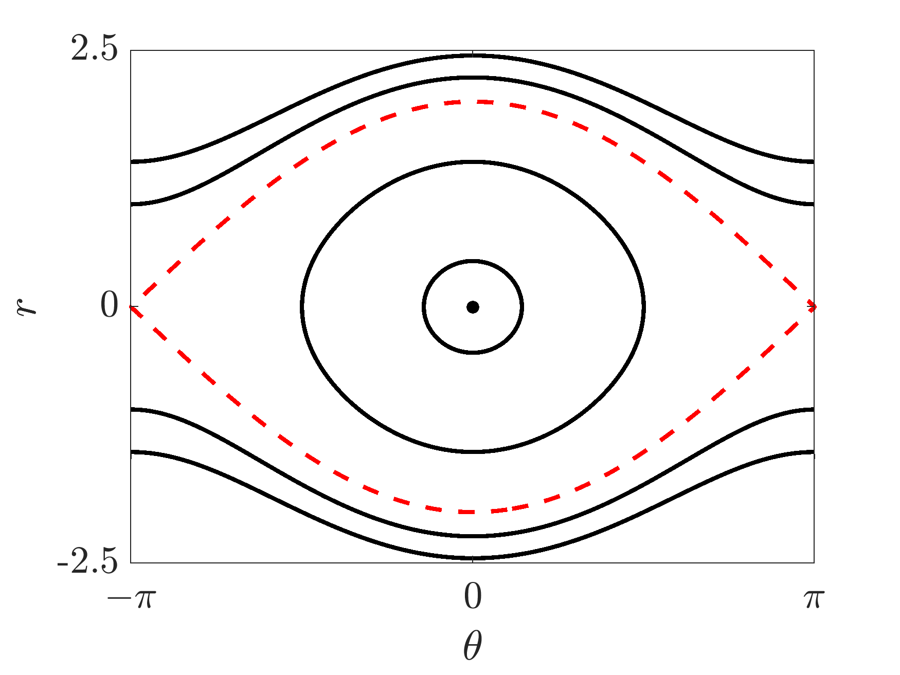
Figure 1. Phase space of the pendulum supporting the cat’s eye separatrix (dashed curve). For $1$-DoF system, the phase space approach allows to introduce a geometrical LD, a natural counterpart of the temporal LD but free of the time variable. The geometrical LD corresponds to the length $\ell(E)$ of the curve associated to the energy level $E$.

We refer to the LD quantity defined in Eq. (1.2) as temporal LD, to emphasize the difference with the geometrical LD just introduced. The geometrical LD has some benefits over the temporal formulation. Firstly, the expression does not rely on the time and the initial Cauchy condition $x_{0}$, but solely on the energy $E$. Secondly, its analytical expression can be derived easily through algebraic manipulators and numerically estimated. In particular, this last step does not rely on the knowledge of the flow (or any approximation of it, e.g., either locally through linearisation or numerical approximation through solvers). Even though the geometrical LD we just introduced resemble its temporal counterpart, in the sense that both quantities are based on the length of orbits, properties of $\ell(E)$ have not been investigated in the LD literature. To this point we now turn our efforts.

Remark 2.2 (Geometrical LD for conservative 1-DoF systems).

The definition of $\ell(E)$ introduced on the pendulum model is general. For example, let us consider a mechanical system for which Newton’s equations are

$$\ddot{x}=-\nabla_{x}V(x),\,x\in\mathcal{I}\subset\mathbb{R},$$ (2.6)

where $V(x)$ denotes a potential energy. The Eq. (2.6) admits the Hamiltonian formulation

$$\mathcal{H}(x,v)=\frac{v^{2}}{2}+V(x),$$ (2.7)

where $v=\dot{x}$. For $E\geq\min_{x}V(x)$, the two branches of the level curves associated to the energy level $E=\mathcal{H}(x,v)$ are given by $v_{\pm}=\pm\sqrt{2(E-V(x))}$. The formula given in Eq. (2.4) becomes

$$\ell(E)=\int\sqrt{1+\frac{(\nabla_{x}V(x)^{2})}{2(E-V(x))}}\,\textrm{d}x,$$ (2.8)

where the integral is computed over a suitable range of the variable $x$.

Remark 2.3 (First integral).

The mechanical systems we discussed have the form “kinetic” plus “potential” energy and the total energy is preserved. If more generally Eq. (1.1) possesses a first integral $I$, i.e., a function $I:\mathcal{D}\to\mathbb{R}$ which satisfies

$$\forall t,\,\forall x\in\mathcal{D},\,I\big{(}\phi^{t}(x)\big{)}=I(x),$$ (2.9)

then, in the case $n=2$, orbits are constrained on the curves which are the level curves of the first integral $I$. The former construction can then be repeated.

2.1. Some properties of $\ell(E)$

The numerical evaluation of the continuous function $E\mapsto\ell(E)$ over the domain $E\in[-2,1]$ is shown in the left panel of Fig. 4. The graph highlights that i) the length reaches a maximum at $E=0$ (the energy labeling the separatrix) and ii) the function $E\mapsto\ell(E)$ is not differentiable at $E=0$ (cusp point). The first statement can be proven rigorously.

Proposition 1.

Consider the pendulum model of Eq. (2.1) and the lengths $\ell(E)$ for $E\geq-2$. The value $\ell(E)$ is maximal on the separatrix, i.e., for $E=0$.

Proof.

For $E\geq 0$, whatever the values of $\theta\in(-\pi,\pi)$, the inequality

$$\frac{\sin^{2}\theta}{2(\cos\theta+E+1)}\leq\frac{\sin^{2}\theta}{2(\cos\theta+1)},$$ (2.10)

hold true. The inequality is preserved by integrating both expressions over $(-\pi,\pi)$ from which we derive $\ell(E)\leq\ell(0)$.

Let us now consider the case $-2\leq E<0$. By exploiting the symmetries of the pendulum, the total length $\ell(E)$ is four times the length of the portion of orbit belonging to the first quadrant, say $\ell_{1}(E)$; our claim will thus be proved once we will prove $\ell_{1}(E_{1})<\ell_{1}(E_{2})$ for all $-2\leq E_{1}<E_{2}<0$. Let us thus fix a positive real $\lambda$, consider the straight line $p=\lambda q$ and its intersection with the level curves with energy $-2\leq E<0$. One can implicitly express the intersection point $q(E)$ as a function of $E$, by considering $\lambda$ a fixed parameter, that is $\lambda^{2}q^{2}=2(E+1+\cos q)$, and thus by geometrical considerations, to conclude that $q(E)$ is an increasing function of $E$. Moreover $q(E)\rightarrow 0$ for $E\rightarrow-2^{+}$ and $q(E)\rightarrow\pi$ for $E\rightarrow 0^{-}$. Let us now consider two values of energy $E_{1}$ and $E_{2}$, such that $-2\leq E_{1}<E_{2}<0$, and let us call $(p_{1},q_{1})$ and $(p_{2},q_{2})$ the intersections points of the straight line with the two energy levels (see Fig. 2).

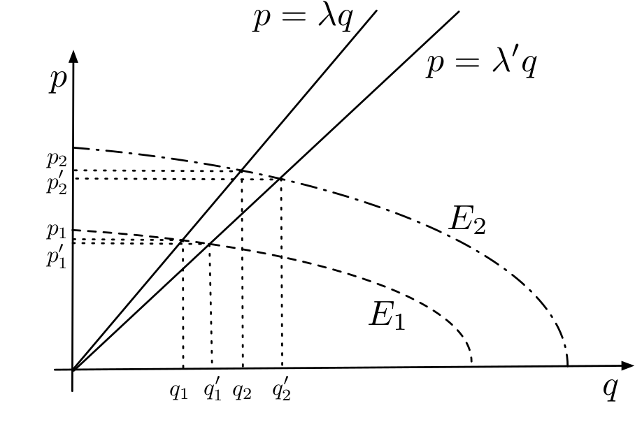
Figure 2. Orbits geometry used in the proof of Propostion 1 in the case $-2\leq E<0$. We reports two level curves associated to two values of the energy $-2\leq E_{1}<E_{2}<0$.

Let us now fix a second positive real $\lambda^{\prime}$ and consider again the intersections of the straight line $p=\lambda^{\prime}q$ with the two energy levels; let us denote them by $(p^{\prime}_{1},q^{\prime}_{1})$ and $(p^{\prime}_{2},q^{\prime}_{2})$. If $\lambda$ and $\lambda^{\prime}$ are infinitesimally close, say $\lambda^{\prime}=\lambda+d\lambda$, then (locally) the arc of level curves can be approximated by

$$d\ell_{1}(E_{i})=\sqrt{1+\frac{\sin^{2}q_{i}}{p^{2}_{i}}}dq_{i},$$ (2.11)

where $dq_{i}=q_{i}-q_{i}^{\prime}$, the reason being that the level curves are smooth functions and thus we are approximating the length $\ell_{1}(E_{i})$, i.e., , the integral in Eq. (2.5), with the length of the segment tangent to the curve at $(p_{i},q_{i})$. Our goal is to prove that $d\ell_{1}(E_{i})$ is an increasing function of the energy and from this to conclude that the same property holds true for the macroscopic arc length.

To achieve our goal we have to express $dq_{1}$ in terms of $dq_{2}$. The first step is to relate $dp_{1}$, $dq_{1}$ and $d\lambda$. By exploiting the linear relation existing between $p_{1}$ and $q_{1}$ we get

$$dp_{1}=\lambda dq_{1}+q_{1}d\lambda,$$ (2.12)

and by recalling that $(p_{1},q_{1})$ belongs to the level curve we also get

$$dp_{1}=-\frac{\sin q_{1}}{p_{1}}dq_{1}.$$ (2.13)

Hence

$$d\lambda=-\left(\frac{\sin q_{1}}{p_{1}}+\lambda\right)\frac{dq_{1}}{q_{1}}.$$ (2.14)

Similar relations hold true for $dp_{2}$, $dq_{2}$ and $d\lambda$, we can then eliminate the dependence from $d\lambda$ and obtain

$$\frac{dq_{2}}{q_{2}}\left(\frac{\sin q_{2}}{p_{2}}+\lambda\right)=\left(\frac{\sin q_{1}}{p_{1}}+\lambda\right)\frac{dq_{1}}{q_{1}}.$$ (2.15)

Recalling the expression Eq. (2.11) for $d\ell_{1}(E_{i})$, after some algebraic manipulations, we can eventually get

$$\frac{d\ell_{1}(E_{1})}{d\ell_{1}(E_{2})}=\frac{\sqrt{q_{1}^{2}\lambda^{2}+\sin^{2}q_{1}}}{\lambda^{2}q_{1}+\sin q_{1}}q_{1}\frac{\lambda^{2}q_{2}+\sin q_{2}}{\sqrt{q_{2}^{2}\lambda^{2}+\sin^{2}q_{2}}}\frac{1}{q_{2}}\equiv F_{\lambda}(q_{1})\frac{1}{F_{\lambda}(q_{2})},$$ (2.16)

where the function $F_{\lambda}(q)$ has been defined by this last equality.

Because of the above mentioned properties of $q_{i}$ as function of $E_{i}$, we can easily show that $F_{\lambda}\rightarrow 0$ for $q\rightarrow 0$ and $F_{\lambda}(\pi)=\pi/\lambda$. By observing the numerical behaviour of the function $F_{\lambda}(q)$ (see Fig. 3) one can conclude that it is monotone increasing for $q\in[0,\pi]$.

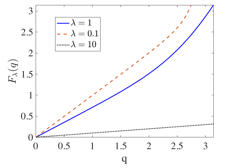
Figure 3. Graph of the function $F_{\lambda}(q)$ for three values of $\lambda$, $0.1$ (red dashed line), $1$ (blue solid line) and $10$ (black dotted line). One can appreciate the monotone increasing behaviour of the function in the domain $[0,\pi]$.

By summarising the last result concerning $F_{\lambda}(q)$ together with the previous one stating that $q_{1}<q_{2}$ if $-2\leq E_{1}<E_{2}<0$, allows to conclude that $d\ell_{1}(E_{1})<d\ell_{1}(E_{2})$. Being this last result independent from the parameter $\lambda$ we can conclude that the length of the energy level $E_{1}$ is smaller than the one associated to the energy $E_{2}$. ∎

Establishing the loss of regularity of $\ell(E)$ at $E=0$ analytically is not a straightforward task, even if this property can be easily appreciated by computing the graph of the function. Interestingly enough, there is also a loss of regularity of the temporal LDs when crossing the separatrix as exemplified on the right panel of Fig. 4. Whilst the length of $\ell(E)$ reaches a global maximum at $E=0$, $\textrm{LD}(r_{0})$ is a local minimum on the line $(r_{0},\theta_{0}=0)$ when $r_{0}$ hits the separatrix at $r(\theta_{0})=2$. The temporal LDs have been computed over the time window $[0,20]$ (by approximating the flow with numerical solvers). We emphasize that the landscape presented in the left panel of Fig. 4 depends solely on the energy, whilst the landscape presented in the right panel has required to compute the LDs over a specific direction (here by freezing the $\theta$ coordinate). The graph of $\ell(E)$ suggests that the separatrix of the pendulum can be delineated and reconstructed semi-analytically, without the knowledge of the flow (or any approximation of it). In fact, each point $(r,\theta)\in\mathcal{D}$ defines a specific energy level $E$ for which $\ell(E)$ follows. Let us stress again that the derivation of $\ell(E)$ does not involve the time parameter whatsoever. The Fig. 5 presents the dynamical maps obtained on $\mathcal{D}=[-2.5,2.5]\times[-\pi,\pi]$, partitioned into a $500\times 500$ Cartesian mesh of coordinates $(r,\theta)$. Let us observe that this approach is redundant and used only to compare with the temporal LD, indeed we could have used points located onto a line transverse to the flow and then associate the computed value of the geometrical LD to all the points lying on the same energy level. From the computation of the geometrical LD on the nodes of this grid, we extracted also the norm of the directional derivatives with respect to the coordinates $(r,\theta)$

$$B(r,\theta)=\left\lVert(\partial_{r}\ell(E),\partial_{\theta}\ell(E))\right\rVert_{2}.$$ (2.17)

Both dynamical maps succeed in revealing the separatrix.

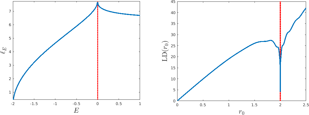
Figure 4. Landscapes of the geometrical and temporal LD on the pendulum model. (Left) The function $\ell$ as a function of $E$ spanning the librational and circulational domains. (Right) Landscape of the temporal LDs computed at $t=20$ along the line of initial condition $(r_{0},\theta_{0}=0)$ where $r_{0}$ spans the librational and circulational domains. In each case, the red dashed vertical lines indicate the location of the separatrix.

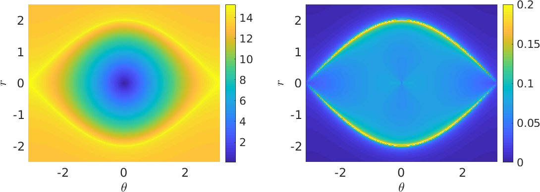
Figure 5. (Left) Dynamical map of the pendulum model obtained by computing $\ell(E)$ and (Right) the norm of its gradient $B$ with respect to $(r,\theta)$.

2.2. Rate of divergence of $|\textrm{d}\ell(E)/\textrm{d}E|$

In this subsection, we take advantage of the geometrical LD in order to quantify the rate at which $|\textrm{d}\ell(E)/\textrm{d}E|$ becomes singular when $E\to E_{\textrm{sx}}=0$. We then connect and discuss the estimate to temporal LDs obtained under linearisation of the flow.

Even if we are interested in energy values close to $E=E_{\textrm{sx}}=0$, let us observe the following fact when $E$ tends to the energy associated to the elliptic point, $E_{\textrm{ell.}}=-2$.

Proposition 2.

Let us consider $E\to-2^{+}$. Then we have $|\textrm{d}\ell(E)/\textrm{d}E|\to+\infty$ at a rate $\mathcal{O}(1/\sqrt{E})$.

Proof.

The linearised Hamiltonian of Eq. (2.1) near the origin reads

$$\mathcal{H}=\frac{r^{2}}{2}+\frac{\theta^{2}}{2}-2.$$ (2.18)

The flow generates solutions which are circles, each circle is labelled by the value of the energy. The radius of the circles are $\textrm{r}=\sqrt{2(E+2)}$. Therefore, $\ell(E)=2\pi\textrm{r}=2\pi\sqrt{2(E+2)}$ and $\textrm{d}\ell(E)/\textrm{d}E=2\pi/\sqrt{2(E+2)}$. ∎

Prop. 2 highlights that the geometrical LDs become singular when approaching the elliptic point. It turns out that the scaling of $|\textrm{d}\ell(E)/\textrm{d}E|$ as $\mathcal{O}(1/\sqrt{E})$ just found in the vicinity of the elliptic point is also valid locally near the saddle point and more generally when $E\to 0$.

Proposition 3.

Let us consider the harmonic repulsor $\mathcal{H}=(r^{2}-\theta^{2})/2$. Then we have $\textrm{d}\ell(E)/\textrm{d}E=\mathcal{O}(1/\sqrt{|E|})$.

Proof.

Given the symmetries, we focus on $r\geq 0,\theta\geq 0,E>0$. For a given $E$, we interpret the finite branch of the hyperbola stemming from $(0,\sqrt{2E})$ as the parametric curve $t\mapsto\big{(}\theta(t),r(t)\big{)}=(\sqrt{2E}\sinh t,\sqrt{2E}\cosh t)$, $t\in[0,t_{\star}]$. The length of this curve is given by

$$\ell(E)=\int_{0}^{t_{\star}}\sqrt{\dot{\theta}^{2}(t)+\dot{r}^{2}(t)}\,\textrm{d}t=\sqrt{2E}\int_{0}^{t_{\star}}\sqrt{\sinh^{2}(t)+\cosh^{2}(t)}\,\textrm{d}t.$$ (2.19)

It follows that $\ell(E)=\sqrt{2E}\kappa(t_{\star})$ and thus

$$\frac{\textrm{d}\ell(E)}{\textrm{d}E}=\frac{1}{\sqrt{E}}\frac{1}{\sqrt{2}}\kappa(t_{\star}).$$ (2.20)

∎

Proposition 4.

Let us consider $E\to E_{\textrm{sx}}=0$. Then we have $|\textrm{d}\ell(E)/\textrm{d}E|\to+\infty$ at a rate $\mathcal{O}(1/\sqrt{|E|})$.

Proof.

(Semi-analytical) We numerically estimate $\ell(E)$ when $E\to 0$ both from the librational ($E\to 0^{-}$) and circulational ($E\to 0^{+}$) domains. Fig. 6 compares the predicted estimates with the numerical estimations of $|\textrm{d}\ell(E)/\textrm{d}E|$ and corroborate the claim. ∎

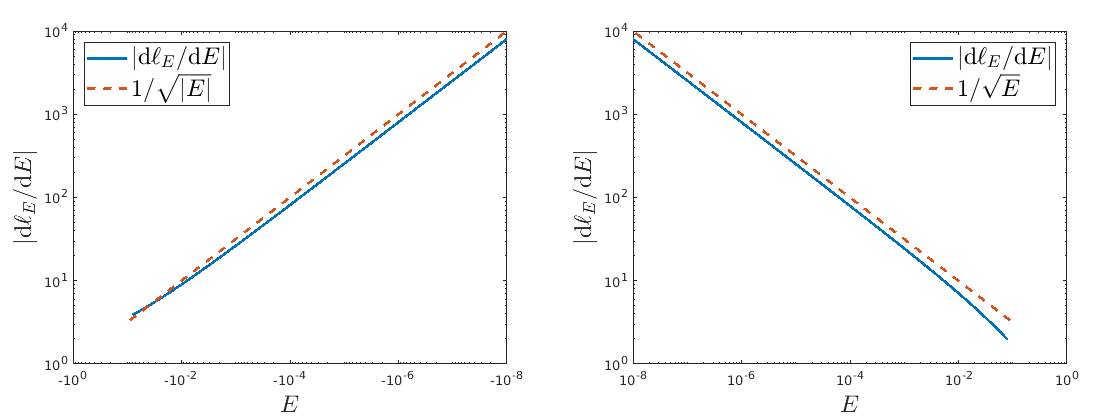
Figure 6. The divergence of $\textrm{d}\ell(E)/\textrm{d}E$ scales as $1/\sqrt{|E|}$ when approaching the separatrix from the librational (left) and circulational (right) domains.

We might wonder if these power-law divergences are encapsulated into the temporal LDs. The following propositions show that a compatible estimate can be recovered near the elliptic and saddle points.

Proposition 5.

Consider the harmonic oscillator $\mathcal{H}=(r^{2}+\theta^{2})/2$. For $t>0$ fixed, we have

$$\frac{\textrm{d}}{\textrm{d}E}\rm{LD}\big{(}(r,\theta);t\big{)}=\mathcal{O}(1/\sqrt{E}).$$ (2.21)

Proof.

Following Mancho et al., (2013) (confer section $2.2.1$), given $(r,\theta)$ and $t>0$, straightforward computations give

$$\rm{LD}\big{(}(r,\theta);t\big{)}=2t\sqrt{r^{2}+\theta^{2}}=2t\sqrt{E},$$ (2.22)

from which the announced equality follows. ∎

Proposition 6.

Consider the harmonic repulsor $\mathcal{H}=(r^{2}-\theta^{2})/2$. For $t>0$ fixed, we have

$$\frac{\textrm{d}}{\textrm{d}E}\rm{LD}\big{(}(r,\theta);t\big{)}=\mathcal{O}(1/\sqrt{E}).$$ (2.23)

Proof.

Given the Cauchy initial condition $(r_{0},\theta_{0})$ at time $t_{0}$, the solutions read

$$\left\{\begin{aligned} &r(t)=p_{0}\cosh(t)+q_{0}\sinh t,\\ &\theta(t)=p_{0}\sinh(t)+q_{0}\cosh t.\end{aligned}\right.$$ (2.24)

Due to the symmetries, one might generically take initial conditions in the first quadrant and write $(q_{0},p_{0})=(\sqrt{2E}\cosh t_{0},\sqrt{2E}\sinh t_{0})$. Then Eq. (2.24) becomes

$$\left\{\begin{aligned} &r(t)=\sqrt{2E}\cosh(t+t_{0}),\\ &\theta(t)=\sqrt{2E}\sinh(t+t_{0}).\end{aligned}\right.$$ (2.25)

We have

$$\textrm{LD}(r_{0},\theta_{0};t)=\int_{0}^{t}\sqrt{\dot{r}^{2}(s)+\dot{\theta}^{2}(s)}\textrm{d}s=\sqrt{2E}\kappa(t)$$ (2.26)

from which follows the equality announced. ∎

3. Geometric Lagrangian descriptors for Duffing’s oscillator

We repeat our previous steps on Duffing’s Hamiltonian model

$$\mathcal{H}=\frac{y^{2}}{2}-\frac{x^{2}}{2}+\frac{x^{4}}{4},\,(x,y)\in\mathbb{R}^{2},$$ (3.1)

supporting an $8$-shaped separatrix. All trajectories are bounded, the phase space is shown in Fig. 7. The equilibrium $(x,y)=(0,0)$ is a saddle (with the corresponding energy $\mathcal{H}(0,0)=0$) and both equilibria $(x,y)=(0,\pm 1)$ are elliptic. Given the symmetry of the phase space, if we restrict the domain to $x\geq 0$ and $y\geq 0$, we interpret the orbits as the planar curves, parametrised by $x$, defined by

$$y(x;E)=\frac{1}{\sqrt{2}}\sqrt{-x^{4}+2x^{2}+4E}.$$ (3.2)

By applying formula given in Eq. (2.4) to Eq. (3.2) leads to

$$\tilde{\ell}(E)=\int_{\mathcal{D}_{E}}\sqrt{1+\frac{2(x-x^{3})^{2}}{-x^{4}+2x^{2}+4E}}\,\textrm{d}y,$$ (3.3)

where

$$\left\{\begin{aligned} &\mathcal{D}_{E}=[0,(1+\sqrt{1+4E})^{1/2}],\,\textrm{if}\ E<0,\\ &\mathcal{D}_{E}=[x_{1},x_{2}],\textrm{otherwise}\end{aligned}\right.$$

with

$$x_{1}=\sqrt{1-\sqrt{1+4E}},\,x_{2}=\sqrt{1+\sqrt{1+4E}}.$$ (3.4)

With this set of formulas, we have $\ell(E)=4\tilde{\ell}(E)$.

The panel in Fig. 8 presents the observables considered in section 2. The length $\ell(E)$ is a local maximal in the vicinity of the separatrix $E=0$, where again $\ell(E)$ is not differentiable. This property underpins the ability to reconstruct the phase space via the length $\ell(E)$ and the $B$ map. Although we are not able to demonstrate analytically the form of the divergence, the semi-analytical apparatus provides evidence that $|\textrm{d}\ell(E)/\textrm{d}E|$ scales again as $\mathcal{O}(1/\sqrt{|E|})$ when $E\to 0$ where the temporal LD cannot be straightforwardly estimated.

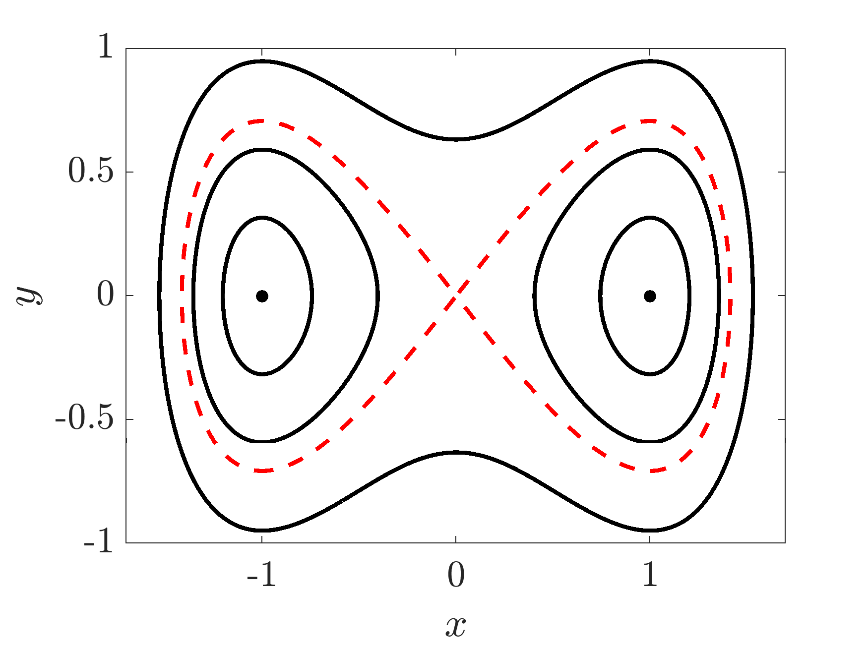
Figure 7. Phase space of Duffing’s oscillator supporting the $8$-shaped separatrix.

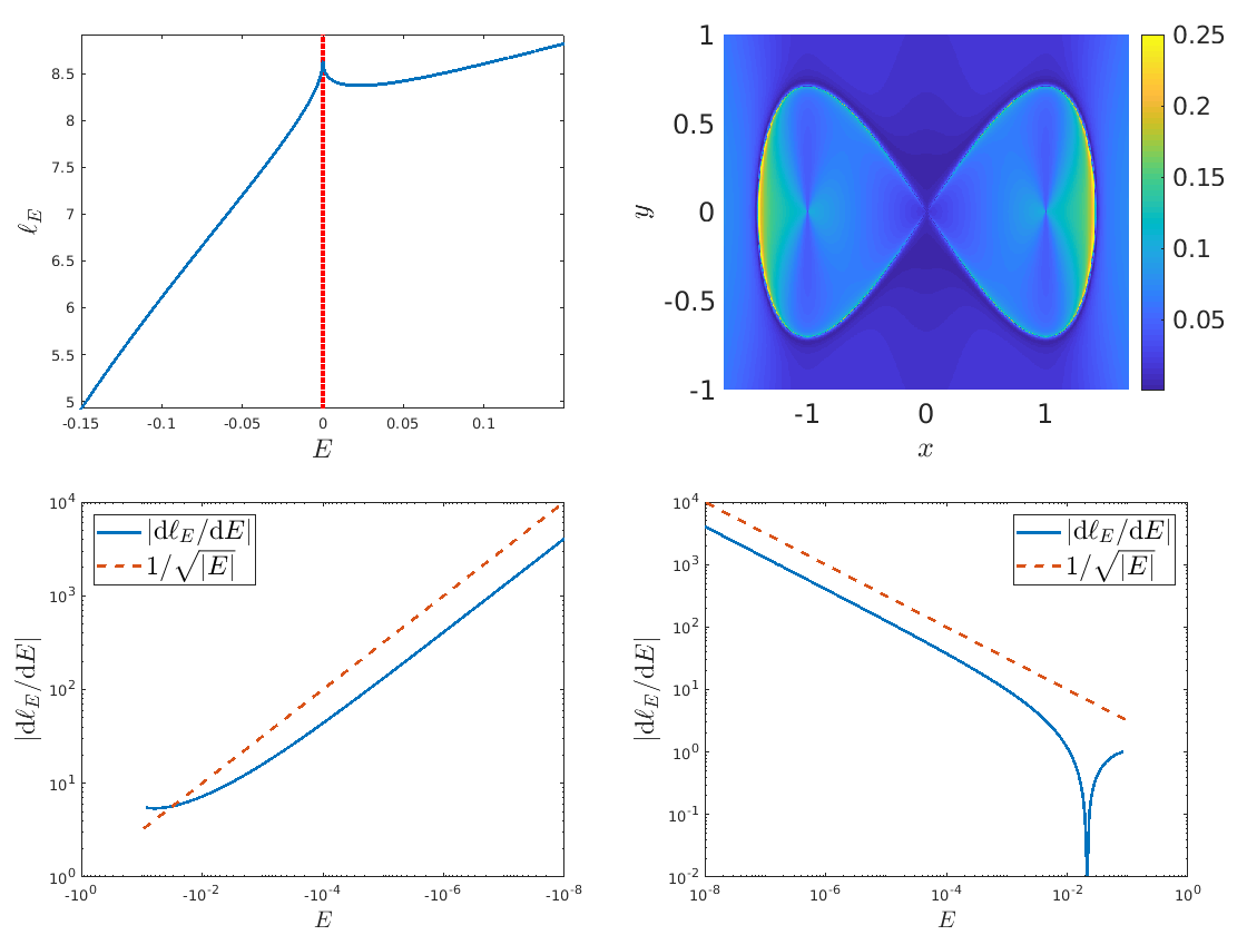
Figure 8. $\ell(E)$ as a function of $E$, $B$ map, and divergence laws associated to Duffing’s oscillator.

4. Geometric Lagrangian descriptors for the fish-tail separatrix

We now turn our attention to the model

$$\mathcal{H}=y^{2}+x^{3}+6x^{2}-32,\,(x,y)\in\mathbb{R}^{2},$$ (4.1)

supporting a fish-tail separatrix and unbounded motions, as shown by the level sets of Fig. 9. The phase space contain two equilibrium, the unstable point $(x,y)=(-4,0)$ and the elliptic fixed point at $(x,y)=(0,0)$. Contrarily to the former models, all values of $E$ lead to $\ell(E)=+\infty$. This can be easily understood by observing that any energy level, also the one associated to librations, contains an unbounded branch. In order to deal with a finite value of $\ell(E)$, we first “artificially” bound the configuration space and allow the $x$ variable to a closed interval $\mathcal{I}=[a,b]\subset\mathbb{R}$. Given the symmetry of the phase space, for $x\in\mathcal{I}$ and $y\geq 0$, the level curves are interpreted as the planar curves

$$y(x;E)=\sqrt{-x^{3}-6x^{2}+E+32}.$$ (4.2)

Formula (2.4) becomes

$$\tilde{\ell}(E)=\int_{\mathcal{D}_{E}}\sqrt{1+\frac{(-3x^{2}-12x)^{2}}{4(-x^{3}-6x^{2}+E+32)}}\,\textrm{d}y.$$ (4.3)

Let us now clarify the domain $\mathcal{D}_{E}$. For circulational orbits ($E>0$), we have

$$\mathcal{D}_{E}=[x_{1},x_{2}],$$ (4.4)

where $x_{1}=a$ and $x_{2}=p^{1/3}+4p^{-1/3}-2$ where

$$p=\frac{1}{2}\sqrt{E(E+32)}+\frac{1}{2}(E+32)-8.$$ (4.5)

For librational orbits, we have

$$\mathcal{D}_{E}=[x_{1},x_{2}]\cup[x_{3},x_{4}],$$ (4.6)

where $x_{1}=a$ and $\{x_{2},x_{3},x_{4}\}$ are the roots, ordered in increasing values, of the polynom $P\in\mathbb{R}^{3}[X]$ given by $P_{E}(X)=-X^{3}-6X^{2}+E+32$. Under this set of formulas, we have $\ell(E)=2\tilde{\ell}(E)$.

The landscape $\ell(E)$ as a function of $E$, $B$ map and divergence laws are shown in Fig. 10. For this particular set of computations, we considered $a=-5$. As for the pendulum and Duffing’s models, $\ell(E)$ reaches a local maximum on the separatrix $E=0$ and forms a cusp point. The B map is thus able to delineate the separatrix. By using the formula presented, we find again that the divergence laws scale as $\mathcal{O}(1/\sqrt{|E|})$. Those observations rely a priori on the choice $a$, however, we have been able to reproduce them by considering a finite number of points $\{a_{i}\}_{i}$ such that $a_{i}\to-\infty$. Alternatively, we can limit our analysis to the case of ”bounded librations” with $E\leq 0$ and $x\geq-4$ and study the finite lengths $\ell(E)$.

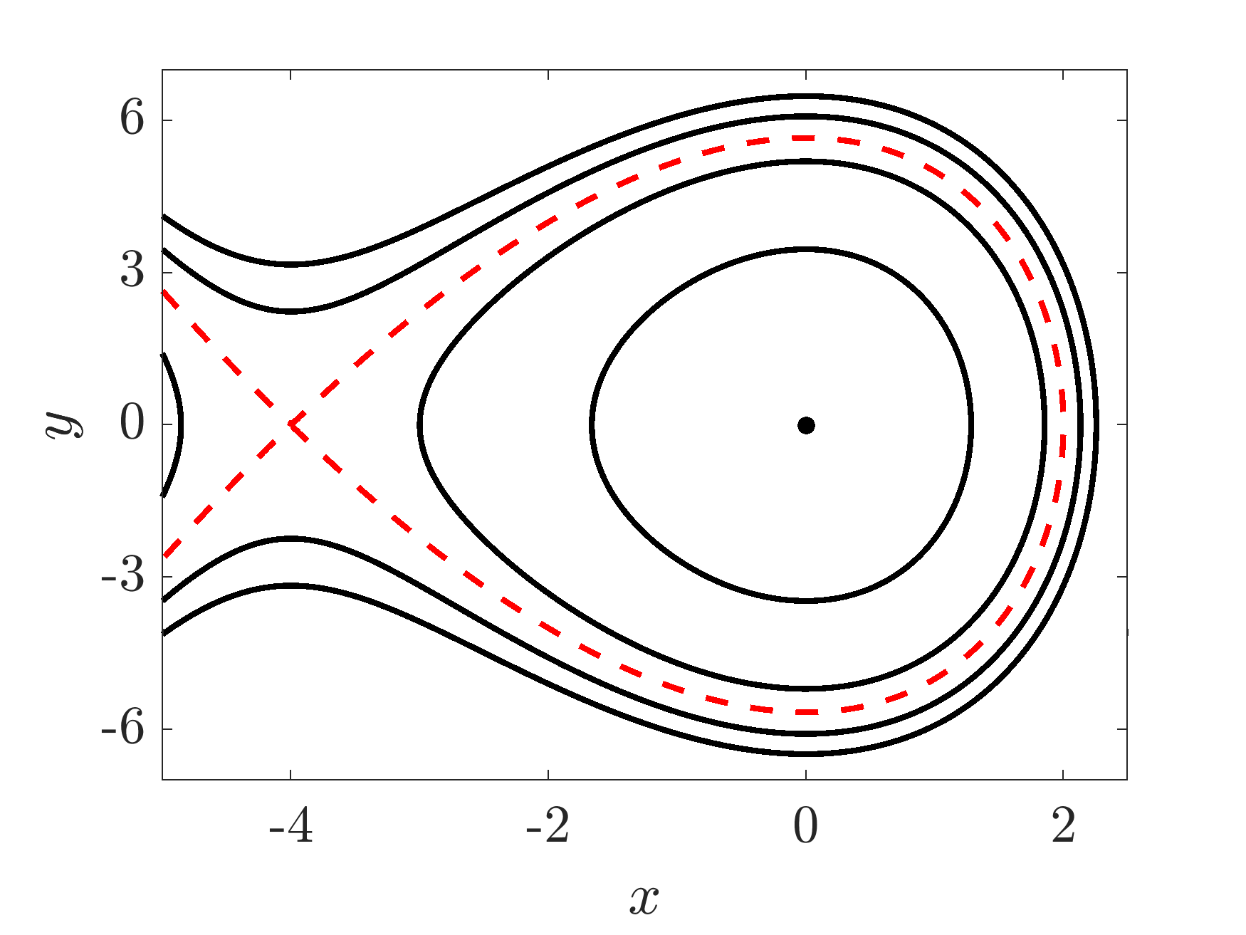
Figure 9. Fish-tail separatrix supporting unbounded motions.

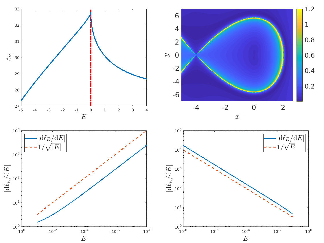
Figure 10. $\ell(E)$ as a function of $E$, $B$ map, and divergence laws associated to the model in Eq. (4.1) supporting a fish-tail separatrix.

5. Conclusion

Leveraging on the classical Lagrangian Descriptors for autonomous vector fields, this work has introduced a geometrical parametrisation for 1 degree-of-freedom system having the energy as first integral. The geometrical Lagrangian Descriptor corresponds to the length $\ell(E)$ of the level curve labeled by the energy level $E$. It has a clear physical interpretation and is in particular free of the time variable. We have discussed applications of this framework on several and classical potential systems supporting the cat’s eye, 8-shaped and fish-tail separatrices. For the models investigated, we have found the indicator to be a local maximum and cusp point on the energy labeling the separatrix. Alike the method of painting the energy integral over the phase space, the properties of the length metric permit to delineate successfully the separatrices of dynamical systems. In addition to providing geometrical insights on the mechanisms driving Lagrangian Descriptors, the apparatus has also conveniently allowed to characterise the rate at which $|\textrm{d}\ell(E)/\textrm{d}E|$ becomes singular near critical energies. Independent of the topology of the separatrices, we have revealed power-laws scaling as $\mathcal{O}(1/\sqrt{|E|})$.

References

- Carlo and Borondo, (2020) Carlo, G. G. and Borondo, F. (2020). Lagrangian descriptors for open maps. Physical Review E, 101(2):022208.
- Carlo et al., (2021) Carlo, G. G., Montes, J., and Borondo, F. (2021). Lagrangian descriptors for the Bunimovich stadium billiard. arXiv preprint arXiv:2110.03739.
- Coffey et al., (1990) Coffey, S., Deprit, A., Deprit, E., and Healy, L. (1990). Painting the phase space portrait of an integrable dynamical system. Science, 247(4944):833–836.
- Craven et al., (2017) Craven, G. T., Junginger, A., and Hernandez, R. (2017). Lagrangian descriptors of driven chemical reaction manifolds. Physical Review E, 96(2):022222.
- Crossley et al., (2021) Crossley, R., Agaoglou, M., Katsanikas, M., and Wiggins, S. (2021). From Poincaré maps to Lagrangian descriptors: The case of the valley ridge inflection point potential. Regular and Chaotic Dynamics, 26(2):147–164.
- Laskar, (1993) Laskar, J. (1993). Frequency analysis of a dynamical system. Celestial Mechanics and Dynamical Astronomy, 56(1):191–196.
- Lopesino et al., (2015) Lopesino, C., Balibrea, F., Wiggins, S., and Mancho, A. M. (2015). Lagrangian descriptors for two dimensional, area preserving, autonomous and nonautonomous maps. Communications in Nonlinear Science and Numerical Simulation, 27(1-3):40–51.
- Lopesino et al., (2017) Lopesino, C., Balibrea-Iniesta, F., García-Garrido, V. J., Wiggins, S., and Mancho, A. M. (2017). A theoretical framework for Lagrangian descriptors. International Journal of Bifurcation and Chaos, 27(01):1730001.
- Madrid and Mancho, (2009) Madrid, J. J. and Mancho, A. M. (2009). Distinguished trajectories in time dependent vector fields. Chaos: An Interdisciplinary Journal of Nonlinear Science, 19(1):013111.
- Mancho et al., (2013) Mancho, A. M., Wiggins, S., Curbelo, J., and Mendoza, C. (2013). Lagrangian descriptors: A method for revealing phase space structures of general time dependent dynamical systems. Communications in Nonlinear Science and Numerical Simulation, 18(12):3530–3557.
- Mendoza et al., (2014) Mendoza, C., Mancho, A., and Wiggins, S. (2014). Lagrangian descriptors and the assessment of the predictive capacity of oceanic data sets. Nonlinear Processes in Geophysics, 21(3):677–689.
- Mendoza and Mancho, (2010) Mendoza, C. and Mancho, A. M. (2010). Hidden geometry of ocean flows. Physical review letters, 105(3):038501.
- Naik et al., (2019) Naik, S., García-Garrido, V. J., and Wiggins, S. (2019). Finding NHIM: Identifying high dimensional phase space structures in reaction dynamics using lagrangian descriptors. Communications in Nonlinear Science and Numerical Simulation, 79:104907.
- Revuelta et al., (2019) Revuelta, F., Benito, R., and Borondo, F. (2019). Unveiling the chaotic structure in phase space of molecular systems using Lagrangian descriptors. Physical Review E, 99(3):032221.
- Skokos, (2010) Skokos, C. (2010). The Lyapunov characteristic exponents and their computation. In Dynamics of Small Solar System Bodies and Exoplanets, pages 63–135. Springer.