Self-lensing flares from BH binaries II:
observing black hole shadows via light curve tomography
Abstract
Supermassive black hole (BH) binaries are thought to produce self-lensing flares (SLF) when the two BHs are aligned with the line-of-sight. If the binary orbit is observed nearly edge-on, we find a distinct feature in the light curve imprinted by the relativistic shadow around the background (”source”) BH. We study this feature by ray-tracing in a binary model and predict that 1% of the current binary candidates could show this feature. Our BH tomography method proposed here could make it possible to extract BH shadows that are spatially unresolvable by high-resolution VLBI.
I Background
Supermassive black hole binaries (SMBHBs) are thought to reside in the cores of many galaxies, as a result of galaxy mergers (Begelman et al., 1980). Their immediate surroundings consist of a circumbinary disk that transfers material to two minidisks, each orbiting one BH component. If the viewing angle with respect to the orbital plane is close to edge-on, a minidisk can get lensed by the foreground BH resulting in a self-lensing flare (SLF) (D’Orazio and Di Stefano, 2018; Ingram et al., 2021), especially in the case of ultra-compact binaries close to merger, in the regime where their gravitational wave (GW) emission is detectable by LISA Haiman (2017).
Observational evidence of SLFs is sparse, a first candidate was identified by Hu et al. (2020) in the optical Kepler data, KIC-11606854 (dubbed ”Spikey”). A second candidate, identified in X-rays, was discussed by Ingram et al. (2021). More generally, quasi-periodic modulations in the light curve of AGN indicating the presence of a SMBHB have recently been found in large optical time-domain surveys (Graham et al., 2015; Charisi et al., 2016; Liu et al., 2019, 2020; Chen et al., 2020).
The first attempts of modeling SLFs were made by using a point source approximation for the lens and the source, with the amplification factor derived from microlensing (Haiman, 2017; D’Orazio and Di Stefano, 2018; Hu et al., 2020). These models are computationally cheap, but they lack general relativistic (GR) effects, and do not take finite source sizes into account. Ref. (D’Orazio and Di Stefano, 2018) also studied the impact of finite source size, but their emission morphology, lacks the strong bending of light close to the BH since GR is not taken into account. Refs. Ingram et al. (2021) and Pihajoki et al. (2018) used general-relativistic ray tracing (GRRT) to study SLFs, but this was either limited to a single mass ratio q=0.01 Pihajoki et al. (2018) or aimed at a single source and only considered circular equal-mass binaries Ingram et al. (2021). Pihajoki et al. (2018) used a superimposed binary metric, while Ingram et al. (2021) used an image of a BH as a faraway image lensed by a single Kerr BH. See also for various applications of lensing in compact binaries (Jaroszynski et al., 1992; Béky and Kocsis, 2013; Bohn et al., 2015; Kelly et al., 2017; d’Ascoli et al., 2018; Schnittman et al., 2018).
In single BH emission models, there is typically a flux depression present in the apparent image. In the optically thin case, this ”hole” in the image coincides with the BH shadow (BHS) Luminet (1979); Falcke et al. (2000); Bronzwaer et al. (2021), while in the optically thick case, the position of the lensed event horizon or the inner-shadow Gralla et al. (2019); Chael et al. (2021). The shadow is a flux depression in the apparent surface brightness, caused by photons being trapped by the event horizon. The first direct observation of such a flux depression or BHS was made by the Event Horizon Telescope (EHT) The Event Horizon Telescope Collaboration et al. (2019). They used very-long baseline interferometry to construct an image of the immediate surrounding of the SMBH in the nucleus of M87. A limitation of direct imaging is that extremely high spatial resolution of -arcseconds was needed to resolve M87*. This limits the potential number of BHs measurable by the current EHT array, although this number is expected to grow with future EHT upgrades (Johnson et al., 2019; Pesce et al., 2021).
In (Davelaar and Haiman, 2021, hereafter Paper I) we present a comprehensive suite of SLF models, obtained via GRRT calculations with our modified version of the GRRT code RAPTOR Bronzwaer et al. (2018, 2020). The code includes a superposed binary metric where the BHs are on Keplerian orbits. The emission is generated by two Novikov-Thorne like (Novikov and Thorne, 1973) minidisks. Each minidisk extends from the horizon or the innermost stable circular orbit (ISCO) to the tidal truncation radius. For full details on the code and model, see Paper I.
In this paper, we investigate substructure found in the SLFs for a subset of models in Paper I. These ”dips” occur when the BHS passes behind the lens. We focus on high-energy emission, which is concentrated in a small region around each BH component, and shares the BH orbital motions, even for the compact binaries of interest Haiman (2017). We generate light curves at 2.5 keV for model parameters affecting the shape of the dip: the inner radii of the minidisks 111Changing the inner radius also changes the velocity profile, Keplerian if at the ISCO or including a radial component if at the event horizon., the binary’s separation , BH spins , disk opacity , and binary inclination . The model parameters are listed in Table 1.
| M0 | 100 | 90 | 0 | thick | |
| M1 | 100 | 90 | 0 | thick | |
| M2 | 100 | 90 | 0 | thin | |
| M3a | 100 | 90 | 0.5 | thick | |
| M3b | 100 | 90 | 0.95 | thick | |
| M4a | 200 | 90 | 0 | thick | |
| M4b | 300 | 90 | 0 | thick | |
| M4c | 400 | 90 | 0 | thick | |
| M4d | 500 | 90 | 0 | thick | |
| M4e | 1000 | 90 | 0 | thick | |
| M5a | 100 | 89 | 0 | thick | |
| M5b | 100 | 88 | 0 | thick | |
| M5c | 100 | 87 | 0 | thick | |
| M5d | 100 | 86 | 0 | thick | |
| M5e | 100 | 85 | 0 | thick | |
| M5f | 100 | 80 | 0 | thick | |
| M6a | 200 | 89 | 0 | thick | |
| M6b | 200 | 88 | 0 | thick | |
| M6c | 200 | 87 | 0 | thick | |
| M6d | 200 | 86 | 0 | thick | |
| M6e | 200 | 85 | 0 | thick | |
| M6f | 200 | 80 | 0 | thick |
II Fiducial self-lensing flare
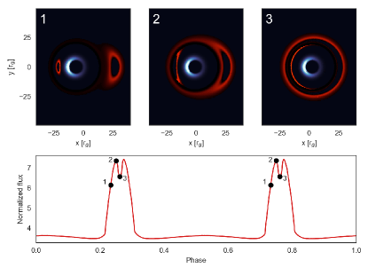
In Figure 1 we show our fiducial model M0. The bottom panel shows the light curve at 2.5 keV that contains two SLFs at a quarter and three-quarters of the orbit. The SLFs have a distinct dip at their peak, which occurs when the BHS passes the lens’ focal point, resulting in a drop in the net amplified flux. The top panels of Figure 1 show synthetic images of model M0 at the start (1), peak (2), and dip (3) of the SLF. A secondary image is visible on the left.
III Parameter dependencies
In model M1, we increase the inner radius, which widens the spacing between the sub-peaks, see Panel 1 of Figure 2. Additionally, since the truncation radius is larger than the photon ring, a second set of sub-flares is visible. The sub-flares have a phase spacing of . Multiplying this value by the total circumference of the orbit (, where is the gravitational radius), we find that this phase difference corresponds to a size of , which is the size of the projected shadow. For guidance, the vertical lines mark the phase duration of the ISCO and photon rings centered on the SLF.
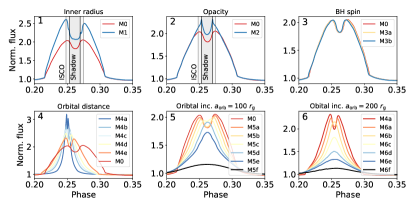
In the optically thin case, model M2, presented in Panel 2 of Figure 2, the main sub-peaks trace the photon ring, since this is the dominant feature in the image. The spacing in phase between the sub-peaks is equal to that for the sub-peaks produced by the photon ring in model M1. We again mark the phase durations of the ISCO and photon rings centered on the middle of the SLF. The dip inside the flare coincides in phase with the shadow’s passage behind the lens.
In models M3a-b, we vary the spin of the BHs (assumed to be the same for both components for simplicity) to and , respectively, compared to non-spinning fiducial case. The light curves of these models are shown in Panel 3 of Fig. 2. The addition of spin results in a slightly smaller and more asymmetric shadow. This is also visible in the light curves; the spacing between the peaks shrinks for increasing spin. However, as the figure shows, the effect of spins is overall very modest.
In models M4a-f we study the dependence on binary separation by changing to , , , and , compared to in the fiducial model. Increasing the separation results in the light curves asymptote to the point source approximation, since the angular size of the source on the sky decreases. Additionally, the source spends a smaller fraction of the orbit within the Einstein radius. In M5a-f we alter the inclination to , , , , and respectively, compared to the fiducial . These light curves are shown in Panel 5 of Fig. 2. The dip is clearly present in models M5a-c, which puts a limit on the range of inclinations for which it can be observed, . In model M6a-f we increase the binary separation to and cover the same span of inclinations. The light curves of these models can be seen in Panel 6 of Fig. 2. As the binary separation increases, the inclination window shrinks to .
IV Analytic expectations
In the case of a perfectly edge-on circular binary, we can derive the expected phase spacing between the two peaks in the optically thin case by taking the ratio between the diameter of the shadow and the circumference of the orbit,
| (1) |
where is the orbital radius, and is diameter of the BHS of the source (Hilbert, 1917; Bardeen, 1973; Luminet, 1979; Falcke et al., 2000), where is related to the full binary mass via . This assumes the source is the secondary BH, which in general is expected to out-accrete and out-shine the primary BH (Farris et al., 2014; Duffell et al., 2020).
The orbital radius is given by , where is the orbital period and is the total binary mass. Combined with Eq. 1 and using geometrized units (), yields
| (2) |
For our fiducial model, , and , which gives , identical to what we found from our light curves. We note that this relation is less trivial for an eccentric binary, since the velocity depends on the nodal angle at which the BHs align and produce the SLF.
Next, we derive an expression for the range of inclination angles . The dip is visible when the focal point of the lens moves over the shadow. This requires that the inclination does not exceed the angular size of the shadow on the sky, or . Using Eq. 1 we then find
| (3) |
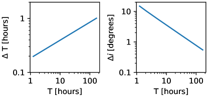
Inserting the fiducial model values, we find , confirming our numerical result from Panel 5 of Fig. 2. In Figure 3 we show the relations for the time interval and the inclination window for a binary with mass where we vary the period. As increases, which is equivalent to increasing the binary separation, the time interval increases, and the inclination window decreases. The spacing of the dip in our fiducial model is . Converting this to physical time for a binary with mass , we find a spacing of 30 minutes. This puts a limit on the time cadence required by an observation (although repeated observations could be phase-folded and reveal the dip in a more coarsely sampled flare). As a function of mass, the orbital period and both scale linearly with mass, making more massive binaries easier to resolve in time.
V Observational limitations
Ideally, individual SLFs should outshine the accretion-induced variability and instrumental noise 222In principle, the periodically recurring SLFs could be discovered via a blind phase folding of the light curve, even if they are individually below the noise.. Typical amplitudes of stochastic AGN variability on timescales of hours to days are 10-40 % in the X-rays (Lawrence and Papadakis, 1993; Maughan and Reiprich, 2019), and 5–10% in the optical on timescales of months (Peterson, 2001). From the inclination-dependent models M25a-f, we find that the flare amplitude exceeds 20% of the unlensed flux when the inclination is larger than . This inclination window for producing 20% flares widens/narrows for more compact/wider binaries (see Fig. 3). The depth of the dip is itself % in the fiducial model, and reduces as the separation increases. The duration of the dip is on the order of hours to days depending on BH mass. The flux variability in AGN typically shows a stochastic red-noise power spectrum (Done et al., 1992; Mushotzky et al., 1993; Vaughan et al., 2003; Panagiotou et al., 2020). This is beneficial since the amplitude of the variability on the short timescales of the SLFs is lower. Additionally, phase-folding can be used to average out stochastic variability.
Large time-domain surveys discovered dozens of candidate SMBHBs based on periodicity in optical light curves (Graham et al., 2015; Charisi et al., 2016), although with sparsely sampled light curves. The estimated BH mass distribution of these candidates is skewed towards the higher BH masses of . This widens the dip’s duration from an hour in our fiducial model to a few days (scaling only the BH mass). By increasing the period of the orbit, this interval would further widen (see Fig. 3) and exceed the five-day cadence for some candidates in (Charisi et al., 2016).
There are some caveats to the detectability of SLFs and their ”dips”. If the image of the source is highly asymmetric, e.g., strongly Doppler-deboosted on one side of the image, the secondary peak we observe in the light curve will be less prominent (Paper I). Using a physical model for the accretion flow, e.g. from hydrodynamic or GR magnetohydrodynamic (GRMHD) simulations, should help clarify the visibility of these features. A recent work d’Ascoli et al. (2018) ray-traced the emission from a binary in GRMHD simulations, and examined the time-averaged bolometric flux as a function of the azimuthal position of an observer at different latitudes. This is an estimate of the phase-folded light curve, and a hint of a dip is visible for nearly edge-on viewing angles (their Fig. 11). The deleterious effects of asymmetric Doppler boosting could also be mitigated if the plane of one (or both) minidisks is misaligned with the binary’s orbital plane. Such misalignment, or related lateral tearing of the minidisks, is possible, if the minidisk orbital angular momentum and BH spin vectors are aligned (Bardeen and Petterson, 1975; Nixon et al., 2011a; Liska et al., 2019), although this configuration is expected to be less common (Gerosa et al., 2015; Nealon et al., 2021).
Another possible limitation is that the edge-on circumbinary disk can block the view to the event horizon. However, the binary orbital plane can be misaligned with respect to the circumbinary disk Nixon et al. (2011a, b); Hayasaki et al. (2013). Furthermore, for thin AGN disks with accretion rates near but below the Eddington limit, with a seperation of , the disk aspect ratio is Haiman et al. (2009), so that the circumbinary disk would not obscure the flare from a coplanar binary.
Finally, compact binaries exhibiting SLFs may be rare because they are short-lived. For instance the GW-driven inspiral time in our fiducial model is a mere 1.5 years ((Peters, 1964), see Eq. 28 in (Haiman et al., 2009)). This is mitigated for larger BH masses since the inspiral time scales linearly with BH mass. For example, a BH would increase the inspiral time by a factor hundred. Additionally, wider binaries are substantially more long-lived since the inspiral time scales with . Wider orbits, which also have wider dips, should ensure that a substantial population is present that might have the right condition for future observations to detect SLFs with BH shadows.
VI Search strategies
An estimation of the probability of observing SLFs was performed by (D’Orazio and Di Stefano, 2018), who estimated that 10% of the currently known SMBHB candidates potentially produce SLFs. These candidates typically have orbital periods of a year and masses of . The visibility of the dip is strongly limited by the orbital inclination, and decreases the probability to observe it. From our formula we find, for the above high-mass candidates, a window of , corresponding to a 1% chance assuming isotropic inclinations. Since 150 candidates are known, one of these could be in the right inclination regime.
Since the probability of detection is low, we propose two strategies to find SLFs with BLS features. First, SLFs could be observable by current and future optical and near-infrared ground-based telescopes, designed for time-domain surveys. One option would be to perform follow-up observations of the already known SMBHB candidates with a daily cadence. Additionally, the Rubin Observatory’s LSST is expected to identify 20-100 million quasars (LSST Science Collaboration et al., 2009; Xin and Haiman, 2021) down to a BH mass of a few . The sheer number of potential sources increases the probability of finding AGNs with the right conditions to measure BHSs, Ref. (Kelley et al., 2021) estimates that hunderds of potential SLFs could be found. The light curves of these quasars will also be sampled at a cadence of a few days, which should be suitable to identify many periodic sources and SLFs.
A second strategy is to perform electromagnetic followups of on-going SMBHB mergers discovered with LISA (Amaro-Seoane et al., 2017). LISA is expected to detect SMBHBs at their late inspiral phase starting at periods of a few hours. At this moment, the binary is already compact (separation Haiman (2017)), which is favorable for observing the BHS since the inclination window increases with decreasing binary period (see Fig. 3). LISA binaries can be identified and localized on the sky to several square degrees 1-2 days prior to their merger Mangiagli et al. (2020), allowing an EM search with wide field-of-view telescopes covering dozens of their orbits. Accurate knowledge of the orbital phase from the GW data will facilitate a concurrent search for SLFs.
VII Summary
We presented numerical models for SLFs in the light curves of SMBHBs, based on GRRT simulations of thin disk emission in an approximate binary metric. If such a SMBHB system is observed close to edge-on, we find a double-peaked substructure in the SLF, where the spacing of the sub-peaks is set by the angular size of the BHS. For our fiducial model the probability of detecting this dip is %, assuming isotropic inclinations. The BH tomography method proposed here would open a new window to discovering BHSs and characterizing their size. The features in the SLFs also yield independent constraints on the BH masses, properties of their emission morphology and kinematics, and the binary’s orbital parameters. Since this method does not require spatially resolving the source, it allows probing BHs which are out of reach for the EHT.
Acknowledgements.
Acknowledgments – The Authors thank Christiaan Brinkerink, Anastasia Gvozdenko, Jeremy Schnittman, and Daniel D’Orazio for valuable comments and discussions during this project. JD is supported by a Joint Columbia/Flatiron Postdoctoral Fellowship. Research at the Flatiron Institute is supported by the Simons Foundation. We acknowledge support by NASA grant NNX17AL82G and NSF grants 1715661 and AST-2006176. Computations were performed on the Popeye computing cluster at SDSC maintained by Flatiron Institute’s SCC. This research has made use of NASA’s Astrophysics Data System. Software: python (Oliphant, 2007; Millman and Aivazis, 2011), scipy (Jones et al., 2001), numpy (van der Walt et al., 2011), matplotlib (Hunter, 2007), RAPTOR (Bronzwaer et al., 2018, 2020).References
- Begelman et al. (1980) M. C. Begelman, R. D. Blandford, and M. J. Rees, Nature 287, 307 (1980).
- D’Orazio and Di Stefano (2018) D. J. D’Orazio and R. Di Stefano, Monthly Notices of the Royal Astronomical Society 474, 2975 (2018).
- Ingram et al. (2021) A. Ingram, S. E. Motta, S. Aigrain, and A. Karastergiou, Monthly Notices of the Royal Astronomical Society 503, 1703 (2021).
- Haiman (2017) Z. Haiman, Phys. Rev. D 96, 023004 (2017), arXiv:1705.06765 [astro-ph.HE] .
- Hu et al. (2020) B. X. Hu, D. J. D’Orazio, Z. Haiman, K. L. Smith, B. Snios, M. Charisi, and R. Di Stefano, Monthly Notices of the Royal Astronomical Society 495, 4061 (2020).
- Graham et al. (2015) M. J. Graham, S. G. Djorgovski, D. Stern, A. J. Drake, A. A. Mahabal, C. Donalek, E. Glikman, S. Larson, and E. Christensen, MNRAS 453, 1562 (2015), arXiv:1507.07603 [astro-ph.GA] .
- Charisi et al. (2016) M. Charisi, I. Bartos, Z. Haiman, A. M. Price-Whelan, M. J. Graham, E. C. Bellm, R. R. Laher, and S. Márka, MNRAS 463, 2145 (2016), arXiv:1604.01020 [astro-ph.GA] .
- Liu et al. (2019) T. Liu, S. Gezari, M. Ayers, W. Burgett, K. Chambers, K. Hodapp, M. E. Huber, R. P. Kudritzki, N. Metcalfe, J. Tonry, R. Wainscoat, and C. Waters, ApJ 884, 36 (2019), arXiv:1906.08315 [astro-ph.HE] .
- Liu et al. (2020) T. Liu, M. Koss, L. Blecha, C. Ricci, B. Trakhtenbrot, R. Mushotzky, F. Harrison, K. Ichikawa, D. Kakkad, K. Oh, M. Powell, G. C. Privon, K. Schawinski, T. T. Shimizu, K. L. Smith, D. Stern, E. Treister, and C. M. Urry, ApJ 896, 122 (2020), arXiv:1912.02837 [astro-ph.HE] .
- Chen et al. (2020) Y.-C. Chen, X. Liu, W.-T. Liao, A. M. Holgado, H. Guo, R. A. Gruendl, E. Morganson, Y. Shen, K. Zhang, T. M. C. Abbott, M. Aguena, S. Allam, S. Avila, E. Bertin, S. Bhargava, et al., MNRAS 499, 2245 (2020), arXiv:2008.12329 [astro-ph.HE] .
- Pihajoki et al. (2018) P. Pihajoki, M. Mannerkoski, J. Nättilä, and P. H. Johansson, The Astrophysical Journal 863, 8 (2018).
- Jaroszynski et al. (1992) M. Jaroszynski, J. Wambsganss, and B. Paczynski, ApJ 396, L65 (1992).
- Béky and Kocsis (2013) B. Béky and B. Kocsis, ApJ 762, 35 (2013), arXiv:1210.4159 [astro-ph.GA] .
- Bohn et al. (2015) A. Bohn, W. Throwe, F. Hébert, K. Henriksson, D. Bunandar, M. A. Scheel, and N. W. Taylor, Classical and Quantum Gravity 32, 065002 (2015), arXiv:1410.7775 [gr-qc] .
- Kelly et al. (2017) B. J. Kelly, J. G. Baker, Z. B. Etienne, B. Giacomazzo, and J. Schnittman, Phys. Rev. D 96, 123003 (2017), arXiv:1710.02132 [astro-ph.HE] .
- d’Ascoli et al. (2018) S. d’Ascoli, S. C. Noble, D. B. Bowen, M. Campanelli, J. H. Krolik, and V. Mewes, ApJ 865, 140 (2018), arXiv:1806.05697 [astro-ph.HE] .
- Schnittman et al. (2018) J. D. Schnittman, T. D. Canton, J. Camp, D. Tsang, and B. J. Kelly, The Astrophysical Journal 853, 123 (2018).
- Luminet (1979) J. P. Luminet, A&A 75, 228 (1979).
- Falcke et al. (2000) H. Falcke, F. Melia, and E. Agol, The Astrophysical Journal 528, L13 (2000).
- Bronzwaer et al. (2021) T. Bronzwaer, J. Davelaar, Z. Younsi, M. Mościbrodzka, H. Olivares, Y. Mizuno, J. Vos, and H. Falcke, MNRAS 501, 4722 (2021), arXiv:2011.00069 [astro-ph.HE] .
- Gralla et al. (2019) S. E. Gralla, D. E. Holz, and R. M. Wald, Phys. Rev. D 100, 024018 (2019), arXiv:1906.00873 [astro-ph.HE] .
- Chael et al. (2021) A. Chael, M. D. Johnson, and A. Lupsasca, ApJ 918, 6 (2021), arXiv:2106.00683 [astro-ph.HE] .
- The Event Horizon Telescope Collaboration et al. (2019) The Event Horizon Telescope Collaboration et al., The Astrophysical Journal 875, L1 (2019).
- Johnson et al. (2019) M. Johnson, K. Haworth, D. W. Pesce, D. C. M. Palumbo, L. Blackburn, K. Akiyama, D. Boroson, K. L. Bouman, J. R. Farah, V. L. Fish, M. Honma, T. Kawashima, M. Kino, A. Raymond, M. Silver, et al., in Bulletin of the American Astronomical Society, Vol. 51 (2019) p. 235, arXiv:1909.01405 [astro-ph.IM] .
- Pesce et al. (2021) D. W. Pesce, D. C. M. Palumbo, R. Narayan, L. Blackburn, S. S. Doeleman, M. D. Johnson, C.-P. Ma, N. M. Nagar, P. Natarajan, and A. Ricarte, arXiv e-prints , arXiv:2108.05228 (2021), arXiv:2108.05228 [astro-ph.HE] .
- Davelaar and Haiman (2021) J. Davelaar and Z. Haiman, arXiv e-prints , arXiv:2112.05828 (2021), arXiv:2112.05828 [astro-ph.HE] .
- Bronzwaer et al. (2018) T. Bronzwaer, J. Davelaar, Z. Younsi, M. Mościbrodzka, H. Falcke, M. Kramer, and L. Rezzolla, Astronomy & Astrophysics 613, A2 (2018).
- Bronzwaer et al. (2020) T. Bronzwaer, Z. Younsi, J. Davelaar, and H. Falcke, Astronomy & Astrophysics 641, A126 (2020).
- Novikov and Thorne (1973) I. D. Novikov and K. S. Thorne, in Black Holes (Les Astres Occlus) (1973) pp. 343–450.
- Note (1) Changing the inner radius also changes the velocity profile, Keplerian if at the ISCO or including a radial component if at the event horizon.
- Hilbert (1917) D. Hilbert, Nachrichten von der Gesellschaft der Wissenschaften zu Göttingen, Mathematisch-Physikalische Klasse 1917, 53 (1917).
- Bardeen (1973) J. M. Bardeen, in Black Holes (Les Astres Occlus) (1973) pp. 215–239.
- Farris et al. (2014) B. D. Farris, P. Duffell, A. I. MacFadyen, and Z. Haiman, ApJ 783, 134 (2014), arXiv:1310.0492 [astro-ph.HE] .
- Duffell et al. (2020) P. C. Duffell, D. D’Orazio, A. Derdzinski, Z. Haiman, A. MacFadyen, A. L. Rosen, and J. Zrake, ApJ 901, 25 (2020), arXiv:1911.05506 [astro-ph.SR] .
- Note (2) In principle, the periodically recurring SLFs could be discovered via a blind phase folding of the light curve, even if they are individually below the noise.
- Lawrence and Papadakis (1993) A. Lawrence and I. Papadakis, ApJ 414, L85 (1993).
- Maughan and Reiprich (2019) B. J. Maughan and T. H. Reiprich, The Open Journal of Astrophysics 2, 9 (2019), arXiv:1811.05786 [astro-ph.HE] .
- Peterson (2001) B. M. Peterson, in Advanced Lectures on the Starburst-AGN, edited by I. Aretxaga, D. Kunth, and R. Mújica (2001) p. 3, arXiv:astro-ph/0109495 [astro-ph] .
- Done et al. (1992) C. Done, G. M. Madejski, R. F. Mushotzky, T. J. Turner, K. Koyama, and H. Kunieda, ApJ 400, 138 (1992).
- Mushotzky et al. (1993) R. F. Mushotzky, C. Done, and K. A. Pounds, ARA&A 31, 717 (1993).
- Vaughan et al. (2003) S. Vaughan, R. Edelson, R. S. Warwick, and P. Uttley, MNRAS 345, 1271 (2003), arXiv:astro-ph/0307420 [astro-ph] .
- Panagiotou et al. (2020) C. Panagiotou, I. E. Papadakis, E. S. Kammoun, and M. Dovčiak, MNRAS 499, 1998 (2020), arXiv:2009.09693 [astro-ph.GA] .
- Bardeen and Petterson (1975) J. M. Bardeen and J. A. Petterson, ApJ 195, L65 (1975).
- Nixon et al. (2011a) C. J. Nixon, P. J. Cossins, A. R. King, and J. E. Pringle, MNRAS 412, 1591 (2011a), arXiv:1011.1914 [astro-ph.HE] .
- Liska et al. (2019) M. Liska, A. Tchekhovskoy, A. Ingram, and M. van der Klis, MNRAS 487, 550 (2019), arXiv:1810.00883 [astro-ph.HE] .
- Gerosa et al. (2015) D. Gerosa, B. Veronesi, G. Lodato, and G. Rosotti, MNRAS 451, 3941 (2015), arXiv:1503.06807 [astro-ph.GA] .
- Nealon et al. (2021) R. Nealon, E. Ragusa, D. Gerosa, G. Rosotti, and R. Barbieri, MNRAS, in press , arXiv:2111.08065 (2021), arXiv:2111.08065 [astro-ph.HE] .
- Nixon et al. (2011b) C. J. Nixon, A. R. King, and J. E. Pringle, MNRAS 417, L66 (2011b), arXiv:1107.5056 [astro-ph.GA] .
- Hayasaki et al. (2013) K. Hayasaki, H. Saito, and S. Mineshige, PASJ 65, 86 (2013), arXiv:1211.5137 [astro-ph.GA] .
- Haiman et al. (2009) Z. Haiman, B. Kocsis, and K. Menou, ApJ 700, 1952 (2009), arXiv:0904.1383 [astro-ph.CO] .
- Peters (1964) P. C. Peters, Physical Review 136, 1224 (1964).
- LSST Science Collaboration et al. (2009) LSST Science Collaboration et al., arXiv e-prints , arXiv:0912.0201 (2009), arXiv:0912.0201 [astro-ph.IM] .
- Xin and Haiman (2021) C. Xin and Z. Haiman, MNRAS 506, 2408 (2021), arXiv:2105.00005 [astro-ph.HE] .
- Kelley et al. (2021) L. Z. Kelley, D. J. D’Orazio, and R. Di Stefano, MNRAS 508, 2524 (2021), arXiv:2107.07522 [astro-ph.HE] .
- Amaro-Seoane et al. (2017) P. Amaro-Seoane, H. Audley, S. Babak, J. Baker, E. Barausse, P. Bender, E. Berti, P. Binetruy, M. Born, D. Bortoluzzi, J. Camp, C. Caprini, V. Cardoso, M. Colpi, J. Conklin, et al., arXiv e-prints , arXiv:1702.00786 (2017), arXiv:1702.00786 [astro-ph.IM] .
- Mangiagli et al. (2020) A. Mangiagli, A. Klein, M. Bonetti, M. L. Katz, A. Sesana, M. Volonteri, M. Colpi, S. Marsat, and S. Babak, Phys. Rev. D 102, 084056 (2020), arXiv:2006.12513 [astro-ph.HE] .
- Oliphant (2007) T. E. Oliphant, Computing in Science & Engineering 9, 10 (2007), https://aip.scitation.org/doi/pdf/10.1109/MCSE.2007.58 .
- Millman and Aivazis (2011) K. J. Millman and M. Aivazis, Computing in Science & Engineering 13, 9 (2011), https://aip.scitation.org/doi/pdf/10.1109/MCSE.2011.36 .
- Jones et al. (2001) E. Jones, T. Oliphant, P. Peterson, et al., “SciPy: Open source scientific tools for Python,” (2001).
- van der Walt et al. (2011) S. van der Walt, S. C. Colbert, and G. Varoquaux, Computing in Science and Engineering 13, 22 (2011), arXiv:1102.1523 [cs.MS] .
- Hunter (2007) J. D. Hunter, Computing in Science and Engineering 9, 90 (2007).