Association study between gene expression and multiple phenotypes in omics applications of complex diseases

Abstract

Studying phenotype-gene association can uncover mechanism of diseases and develop efficient treatments. In complex disease where multiple phenotypes are available and correlated, analyzing and interpreting associated genes for each phenotype respectively may decrease statistical power and lose intepretation due to not considering the correlation between phenotypes. The typical approaches are many global testing methods, such as multivariate analysis of variance (MANOVA), which tests the overall association between phenotypes and each gene, without considersing the heterogeneity among phenotypes. In this paper, we extend and evaluate two p-value combination methods, adaptive weighted Fisher’s method (AFp) and adaptive Fisher’s method (AFz), to tackle this problem, where AFp stands out as our final proposed method, based on extensive simulations and a real application. Our proposed AFp method has three advantages over traditional global testing methods. Firstly, it can consider the heterogeneity of phenotypes and determines which specific phenotypes a gene is associated with, using phenotype specific 0-1 weights. Secondly, AFp takes the p-values from the test of association of each phenotype as input, thus can accommodate different types of phenotypes (continuous, binary and count). Thirdly, we also apply bootstrapping to construct a variability index for the weight estimator of AFp and generate a co-membership matrix to categorize (cluster) genes based on their association-patterns for intuitive biological investigations. Through extensive simulations, AFp shows superior performance over global testing methods in terms of type I error control and statistical power, as well as higher accuracy of 0-1 weights estimation over AFz. A real omics application with transcriptomic and clinical data of complex lung diseases demonstrates insightful biological findings of AFp.

1 Introduction

Identifying genes associated with phenotypes of interest in transcriptomics studies can help understand mechanism of diseases and extensive efforts have been tried . For example, Peters et al. (2015) identified 1197 genes associcated with chronological age using whole-blood gene expression data and Blalock et al. (2004) tested gene expression with MiniMental Status Examination (MMSE) and neurofibrillary tangle (NFT) in Alzheimer’s disease (AD) patients, identifying thousands of genes significantly correlated with two AD markers respectively. One special case is the differentially expressed (DE) analysis where the phenotype of interest is binary (e.g., diease/control). Identifying DE genes and the enriched pathways has become a standard pipeline in modern transcriptomics application and many softwares have been developed (Robinson et al., 2010; Ritchie et al., 2015). However, a complex disease is usually characterized by multiple phenotypes, reflecting different facets of the disease. Take chronic obstructive pulmonary disease (COPD) as an example, the disease can be characterized by multiple phenotypes, such as FEV1 (i.e., the volume of breath exhaled with effort in one second), FVC (i.e., the full amount of air that can be exhaled with effort in a complete breath), and differential test of white blood cells. A naive way is to test the association between each gene and each single phenotype at a time and interpret each set of associated genes. However, it may decrease the statistical power when each phenotype is weakly associated with a gene and lose intepretation by failing to find a common gene set associated with multiple phenotypes. Therefore, how to jointly analyze the association between a gene and multiple phenotypes is the interest of this paper. Below we introduced four remaining challenges in omics applications, followed by a review of existing methods.

The first issue is to identify the genes associated with the phenotypes (i.e, global test). We consider the following union-intersection test (UIT) (Roy, 1953) or conjunction null hypothesis (Benjamini and Heller, 2008) in the statistical literatures for each gene:

$$\begin{array}[]{l}H_{0}:\vec{\theta}\in\bigcap\{\theta_{k}=0\}\\ H_{A}:\vec{\theta}\in\bigcup\{\theta_{k}\neq 0\}\end{array}$$

to determine the overall association between a gene and $K$ phenotypes of interest, where $\theta_{k}$ is the effect size for phenotype $k$, $1\leq k\leq K$. The existing methods to solve this question can be summarized into three categories. The first category includes some classical methods for multivariate data, such as multivariate analysis of variance (MANOVA), linear mixed models (LMMs) and generalized linear models (GLMM). MANOVA and LMMs require Gaussian assumption and cannot be applicable to non-Gaussian phenotypes (e.g., binary and count-based data). GLMM cannot be used when the phenotypes are mixed with more than one data types. We will evaluate MANOVA in this paper. The second category is regression-based methods. O’Reilly et al. (2012) proposed MultiPhen method by regressing genotypes on phenotypes via proportional odds logistic model, which is only applicable to ordinal outcome in GWAS studies. Wu and Pankow (2016) proposed multi-trait gene sequence kernel association test (MSKAT), where the purpose is to test the association between a phenotype and multiple SNPs in a chromesome region and cannot be easily extended to our scenario. Therefore, we don’t include these two regression-based methods into evaluation in this paper.

The third category is to combine summary statistics (e.g., p-values and test statistics) from association test of each phenotype, which has been widely used in meta-analysis field to identify DE genes for multiple studies and GWAS setting with multiple phenotypes. These methods can lead to increased statistical power by combining the summary statistics representing the strength of association between a gene and each phenotype. Moreover, methods by combining p-values can accommodate phenotypes with mixed data types since each p-value can be calculated respectively using different approaches. O’Brien (1984) combined the test statistics from the individual test on each trait weighted by inverse variance. Pan et al. (2014) and Zhang et al. (2014) proposed the sum of powered score tests (SPU) and adaptive SPU (aSPU) to combine the score test statistics derived from generalized estimation equations (GEE) in GWAS settings. We include aSPU into evaluation with two variants, the working correlation matrix of GEE being diagonal (aSPU.ind) or exchangeable (aSPU.ex), where aSPU.ind was used as default in Zhang et al. (2014). Many p-value combination methods were also developed, including Fisher’s method (Fisher, 1992), the minimum p-value method (minP) (Tippett et al., 1931), and many others. Fisher’s method defines the test statistic for each gene as the sum of log-transformed p-values by giving all p-values equal weights: $T^{Fisher}=-2\sum_{k=1}^{K}\log p_{k}$, where $p_{k}$ is the p-value from the test of $k$th phenotype. A larger Fisher’s score indicates stronger association. minP uses the minimum p-value among $p_{1},p_{2},\cdots,p_{K}$ as the test statistic. Under meta-analysis setting, p-values from different studies are independent and the null distribution of Fisher’s and minP method are $\chi^{2}_{2K}$ and beta distribution respectively. In our setting, the phenotypes are correlated and the null distribution can be generated by randomly permuting the sample order for gene expression data, keeping the phenotypes data unchanged, which breaks the association between genes and phenotypes while keeping the correlation among phenotypes. Van der Sluis et al. (2013) proposed to exploit the correlation among p-values from each univariate test and generate a new test statistic (TATES). We include Fisher, minP, and TATES into evaluation.

The second challenge is to characterize heterogeneity across phenotypes. Take Fisher as an example, suppose $K=3$ , $\vec{p}_{1}=(0.001,1,1)$ represents p-values of three phenotypes of Gene 1 and $\vec{p}_{2}=(0.1,0.1,0.1)$ represents p-values of Gene 2. Both genes produce the same Fisher’s statistics ($T^{Fisher}=13.8$), but the biological interpretation of the two genes are obviously different. $\vec{p}_{1}$ indicates strong statistical significance only in the first phenotype, while $\vec{p}_{2}$ shows marginal statistical significance in all three phenotypes. All the methods mentioned above fail to characterize heterogeneity across phenotypes, and to tackle this problem, adaptive Fisher’s method (Song et al., 2016) and adaptive weighted Fisher’s method (Huo et al., 2020) are two applicable methods. Both methods generate 0-1 weights vector $\vec{w}=(w_{1},w_{2},w_{3})$ where $w_{k}=1$ ($1\leq k\leq K$, suppose $K=3$) indicates this phenotype is associated with a gene and 0 otherwise. Both methods are proposed under meta-analysis with independent multiple studies where searching for the optimal weight from the smallest to largest p-value is sufficient. In other words, they ordered p-values ($p_{1},p_{2},p_{3}$) from the smallest to largest to get ordered p-values $(p_{(1)},p_{(2)},p_{(3)})$ and determined the best $\vec{w}$ from $(1,0,0),(1,1,0)$ and $(1,1,1)$. However, in our setting, phenotypes are correlated and we propose to extend these two methods by considering correlation among phenotypes using combinatorial search with the original $(p_{1},p_{2},p_{3})$ and determine the best $\vec{w}$ among $(1,0,0),(0,1,0),(0,0,1),(1,0,1),(0,1,1),(1,1,0)$ and $(1,1,1)$. To simplify notation hereafter, we abbreviate adaptive Fisher’s method Song et al. (2016) as AFz since it utilizes standardized sum statistics as test statistic to determine the optimal weight, and abbreviate adaptive weighted Fisher’s method Huo et al. (2020) as AFp since it uses the p-value of sum statistics as the proposed test statistic. The details of AFz and AFp will be introduced in Section 2.3 and 2.4.

The third issue remained is to estimate the uncertainty of 0-1 weights. Huo et al. (2020) proposed a bootstrapping method to estimate the variability index under independent settings and we borrow the idea in our setting for AFp and AFz. The fourth challenge is to identify clusters of genes as gene modules ($M_{1},M_{2},\cdots M_{q}$). For each two genes $i$ and $j$ within the same gene module, $v_{i}^{k}=v_{j}^{k}$ ($\forall$ $1\leq k\leq K$), where $v_{i}^{k}=w_{i}^{k}$sign($\theta_{i}^{k}$) $\in\{-1,0,1\}$ and sign($\theta_{i}^{k}$) indicates the up-regulation or down-regulation. Given $K$ studies, the resulting genes could be categorized into ($3^{K}-1$) groups. This becomes intractable for further biological investigation when $K$ is large. For example, combining $K=5$ studies produces $35-1=242$ categories of biomarkers. Following Huo et al. (2020), we propose to estimate comembership matrix of genes through bootstrapping, followed by tight clustering method (Tseng and Wong, 2005), to tackle this issue.

AFp and AFz can both be used to determine genes associated with phenotypes, characterize heterogeneity among phenotypes, estimate uncertainy of estimated weights and clustering genes into gene modules, while the performance of AFp and AFz hasn’t been fully studied. In this paper, we systematically evaluate AFp and AFz. Our contributions are two-fold: 1) We use extensive simulation to evaluate the type I error rate and power for AFp, AFz, minP, Fisher, TATES, aSPU.ind and aSPU.ex where AFp and AFz show robust performance in all scenarios. 2) We comprehensively evaluate the performance of AFp and AFz for characterizing heterogeneity (i.e., accuracy of 0-1 weights estimation) and identify AFp as the best performer. Therefore, AFp is the final method we recommend for general purpose of gene-phenotype association analysis and gene categorization. The article is structured as follows. In Section 2, we introduce AFp and AFz methods respectively under settings of correlated phenotypes (Section 2.3 and 2.4), followed by the bootstrapping algorithms to estimate variability index and categorize genes (Section 2.5 and 2.6). Section 3 includes extensively simulations to evaluate AFp, AFz, as well as other existing methods. Section 4 contains the result from a lung disease transcriptomic dataset. We include final conclusion and discussion in Section 5.

2 Methods

In this section, we will introduce AFp and AFz methods, which can determine whether a gene is associated with all the phenotypes, characterize the heterogeoity among phenotypes by 0-1 weights, estimate variability index of weights estimated and cluster genes based on their association pattern with phenotypes. Suppose there are $n$ independent, $K$ phenotypes, $p$ gene features and $M$ covariates. Denote by $y_{ik}$, $z_{im}$ snd $x_{ij}$ the $k$th phenotype, $m$th covariate and $j$th gene feature of subject $i$ respectively, where $1\leq k\leq K$, $1\leq m\leq M$, and $1\leq j\leq p$. $\overrightarrow{\boldsymbol{Y_{k}}}=(y_{1k},y_{2k},\ldots,y_{nk})^{T}$, $\overrightarrow{\boldsymbol{Z_{m}}}=(z_{1m},z_{2m},\ldots,z_{nm})^{T}$, and $\overrightarrow{\boldsymbol{X_{j}}}=(x_{1j},x_{2j},\ldots,x_{nj})^{T}$ are the vectors $k$th phenotype, $m$th covariate or $j$th gene for all the samples.

2.1 Generalized linear models

For both AFp and AFz, a generalized linear model of the following form is assumed for the $k$th phenotype and the $j$th gene with $M$ covariates:

$$g_{k}(E(Y_{ik}))=x_{ij}\cdot\theta_{jk}+\sum_{m=1}^{M}z_{im}\cdot\alpha_{mkj}$$ (1)

where $\theta_{jk}$ is the coefficient of gene featture, $\alpha_{mkj}$ is the coefficient of covariates and $g_{k}()$ is the link function. The associated p-value $p_{jk}$ of $\theta_{jk}$ can be derived by classic Wald test or Score test, which serves as input for AFp and AFz. Considering heterogeity among phenotypes, weighted statistic

$$U_{j}(\overrightarrow{\boldsymbol{w_{j}}})=-\sum_{k=1}^{K}w_{jk}\log(p_{jk})$$

can be used to determine whether $j$th gene is associated with phenotypes, where $w_{jk}\in\{0,1\}$ can tell which phenotypes contribute to the association, $\overrightarrow{\boldsymbol{w_{j}}}=(w_{j1},w_{j2},\ldots,w_{jK})^{T}$ and the searching space $\Omega=\left\{\overrightarrow{\boldsymbol{w_{j}}}:\overrightarrow{\boldsymbol{w_{j}}}\neq 0,\overrightarrow{\boldsymbol{w_{j}}}=\left(w_{j1},\ldots,w_{jK}\right)\in\{0,1\}^{K}\right\}$ contains $2^{K}-1$ non-zero vectors of weights (See Section 2.3 and 2.4 for details). The observed weighted statistic of $U_{j}(\overrightarrow{\boldsymbol{w_{j}}})$ is denoted as $u_{j}(\overrightarrow{\boldsymbol{w_{j}}})$.

2.2 Permutation

Both AFp and AFz are derived from observed weighted statistic $u_{j}(\overrightarrow{\boldsymbol{w_{j}}})$, $1\leq j\leq p$. AFp uitilizes the smallest p-value of $u_{j}(\overrightarrow{\boldsymbol{w_{j}}})$ among all possible weight $\overrightarrow{\boldsymbol{w_{j}}}$ as test statistic while AFz standardizes $u_{j}(\overrightarrow{\boldsymbol{w_{j}}})$ based on mean and standard deviation under null (See Section 2.3 and 2.4). Since the mean, standard deviation and p-value of observed weighted statistics $u_{j}(w_{j})$ are intractable to calculated analytically, permutation methods will be used to generate null distribution of $U_{j}(\overrightarrow{\boldsymbol{w_{j}}})$. We intend to test the conditional independence between each gene and $K$ phenotypes given the covariates $\boldsymbol{Z}$ (i.e., $\boldsymbol{Y}\perp\overrightarrow{\boldsymbol{X_{j}}}\mid\boldsymbol{Z}$), where $\boldsymbol{Z}=(\overrightarrow{\boldsymbol{Z_{1}}},\overrightarrow{\boldsymbol{Z_{2}}},\ldots\overrightarrow{\boldsymbol{Z_{m}}})$ and $\boldsymbol{Y}=(\overrightarrow{\boldsymbol{Y_{1}}},\overrightarrow{\boldsymbol{Y_{2}}},\ldots\overrightarrow{\boldsymbol{Y_{K}}})$. The permutation procedure should break the associations between $\boldsymbol{Y}$ and $\overrightarrow{\boldsymbol{X_{j}}}$ while preserving the associations between $\boldsymbol{Y}$ and $\boldsymbol{Z}$ and between $\overrightarrow{\boldsymbol{X_{j}}}$ and $\boldsymbol{Z}$. Simply permuting the genotype $\overrightarrow{\boldsymbol{X_{j}}}$ leads to inflated type I error rate, because the correlation between $\overrightarrow{\boldsymbol{X_{j}}}$ and covariates $\boldsymbol{Z}$ are also destroyed. Following Potter (2005) and Werft and Benner (2010), we permute residuals of regressions of $\overrightarrow{\boldsymbol{X_{j}}}$ on $\boldsymbol{Z}$ for generalized regression models. That is, we first regress each gene feature on the covariates, then permute the residuals derived from the regression and fit the generalized linear model by regressing each phenotype on the permuted residuals.

Specifically, we denote the vector of residuals of regressing $\boldsymbol{X_{j}}$ on $\boldsymbol{Z}$ as $\overrightarrow{\boldsymbol{e_{j}}}=(e_{1j},e_{2j},\ldots,e_{nj})^{T}$ and permute it for $B$ times. In the $b$th permutation, we regress $\overrightarrow{\boldsymbol{Y}_{k}}$ on $\boldsymbol{e}_{\boldsymbol{j}}^{(b)}$ by generalized linear model $g_{k}(E(Y_{ik}))=e^{(b)}_{ij}\cdot\theta^{(b)}_{jk}$ ($1\leq i\leq n$) and get the p-values $p_{jk}^{(b)}$ for the coefficient $\theta^{(b)}_{jk}$. After $B$ permutations, we get a $B\times K$ matrix $\mathbb{P}=\{p_{jk}^{(b)}\}$. The oberved weighted statistics for permuted data can be derived as $u_{j}^{(b)}(\overrightarrow{\boldsymbol{w_{j}}})=-\sum_{k=1}^{K}w_{jk}\log(p^{(b)}_{jk})$. Note that we break the association of each gene and each phenotype. Therefore, for a given weight $\overrightarrow{\boldsymbol{w_{j}}}$, the null distribution of observed weighted statistic $u_{j}(\overrightarrow{\boldsymbol{w_{j}}})$ is $\{p^{(b)}_{j^{\prime}k},1\leq b\leq B,1\leq j^{\prime}\leq p\}$ with precision $B\times p$.

2.3 AFp

Under the null hypothesis that $\theta_{jk}=0$, $\forall k$. the p-value of observed weighted statistic, $p_{U}(u_{j}(\overrightarrow{\boldsymbol{w_{j}}}))$, can be obtained for $j$th gene and a given weight $\overrightarrow{\boldsymbol{w_{j}}}\in\Omega$ by

$$p_{U}(u_{j}(\overrightarrow{\boldsymbol{w_{j}}}))=\frac{\sum_{b=1}^{B}\sum_{j^{\prime}=1}^{p}I\{u_{j^{\prime}}^{(b)}(\overrightarrow{\boldsymbol{w_{j}}})\geq u_{j}(\overrightarrow{\boldsymbol{w_{j}}})\}}{B\cdot p}$$

and AFp statistic is defined as the minimal p-value among all possible weights $\overrightarrow{\boldsymbol{w_{j}}}\in\Omega$:

$$T_{j}^{\mathrm{AFp}}=\min_{\overrightarrow{\boldsymbol{w_{j}}}\in\Omega}p_{U}(u_{j}(\overrightarrow{\boldsymbol{w_{j}}})).$$

The associate weight vector

$$\overrightarrow{\boldsymbol{w_{j}}}^{AFp}=\arg\min_{\overrightarrow{\boldsymbol{w_{j}}}\in\Omega}p_{U}(u_{j}(\overrightarrow{\boldsymbol{w_{j}}}))$$

can determine heterogeneity of genes (second issue discussed in Section 1) and serve as a convenient basis for gene categorization in follow-up biological interpretations and explorations (third and fourth issue discussed in Section 1). To get the p-value of $T_{j}^{\mathrm{AFp}}$, we similarly calculate $T_{j}^{\mathrm{AFp,(b)}}$ using $\mathbb{P}=\{p_{jk}^{(b)}\}$ from permutation. Specifically, we calculate

$$T_{j}^{\mathrm{AFp,(b)}}=\min_{\overrightarrow{\boldsymbol{w_{j}}}\in\Omega}p_{U}(u^{(b)}_{j}(\overrightarrow{\boldsymbol{w_{j}}})),$$

where $p_{U}(u^{(b)}_{j}(\overrightarrow{\boldsymbol{w_{j}}}))=\frac{\sum_{b=1}^{B}\sum_{j^{\prime}=1}^{p}I\{u_{j^{\prime}}^{(b)}(\overrightarrow{\boldsymbol{w_{j}}})\geq u^{(b)}_{j}(\overrightarrow{\boldsymbol{w_{j}}})\}}{B\cdot p}$ and the p-value of $T_{j}^{\mathrm{AFp}}$ can be calculated as

$$p_{T}(T^{AFp}_{j})=\frac{\sum_{b=1}^{B}\sum_{j^{\prime}=1}^{p}I\{T_{j^{\prime}}^{AFp,(b)}\leq T_{j}^{AFp}\}}{B\cdot p}.$$

In summary, $p_{T}(T^{AFp}_{j})$ can be used to determine whether $j$th gene is associated with $K$ phenotypes and $\overrightarrow{\boldsymbol{w_{j}}}^{AFp}$ can be used to determine which specific phenotypes the $j$th gene is associated with.

2.4 AFz

For a given $\overrightarrow{\boldsymbol{w_{j}}}\in\Omega$, the mean and standard deviation of $u_{j}(\overrightarrow{\boldsymbol{w_{j}}})$ under null are $E(u_{j}(\overrightarrow{\boldsymbol{w_{j}}}))=\frac{\sum_{b=1}^{B}\sum_{j^{\prime}=1}^{p}u^{(b)}_{j^{\prime}}(\overrightarrow{\boldsymbol{w_{j}}})}{B\cdot p}$ and $sd(u_{j}(\overrightarrow{\boldsymbol{w_{j}}}))=\sqrt{\frac{\sum_{b=1}^{B}\sum_{j^{\prime}=1}^{p}\{u_{j^{\prime}}^{(b)}(\overrightarrow{\boldsymbol{w_{j}}})-E(u_{j}(\overrightarrow{\boldsymbol{w_{j}}}))\}^{2}}{B\cdot p}}$ . AFz calculates the standarized observed weighted statistic,

$$u^{\prime}_{j}(\overrightarrow{\boldsymbol{w_{j}}})=\frac{u_{j}(\overrightarrow{\boldsymbol{w_{j}}})-E(u_{j}(\overrightarrow{\boldsymbol{w_{j}}}))}{sd(u_{j}(\overrightarrow{\boldsymbol{w_{j}}}))},$$

and the AFz statistic is defined as the largest standarized observed weighted statistic among all possible weights:

$$T_{j}^{\mathrm{AFz}}=\max_{\overrightarrow{\boldsymbol{w_{j}}}\in\Omega}u^{\prime}_{j}(\overrightarrow{\boldsymbol{w_{j}}})$$

The associate weight vector can be determined as

$$\overrightarrow{\boldsymbol{w_{j}}}^{AFz}=\arg\max_{\overrightarrow{\boldsymbol{w_{j}}}\in\Omega}u^{\prime}_{j}(\overrightarrow{\boldsymbol{w_{j}}})$$

To calculate p-value of $T_{j}^{\mathrm{AFz}}$, we obtain standardized observed weighted statistic of permuted data by $u^{\prime,(b)}_{j}(\overrightarrow{\boldsymbol{w_{j}}})=\frac{u^{(b)}_{j}(\overrightarrow{\boldsymbol{w_{j}}})-E(u^{(b)}_{j}(\overrightarrow{\boldsymbol{w_{j}}}))}{sd(u^{(b)}_{j}(\overrightarrow{\boldsymbol{w_{j}}}))}$ and $T_{j}^{\mathrm{AFz,(b)}}=\max_{\overrightarrow{\boldsymbol{w_{j}}}\in\Omega}u^{\prime,(b)}_{j}(\overrightarrow{\boldsymbol{w_{j}}})$, where $E(u^{(b)}_{j}(\overrightarrow{\boldsymbol{w_{j}}}))=E(u_{j}(\overrightarrow{\boldsymbol{w_{j}}}))$ and $sd(u^{(b)}_{j}(\overrightarrow{\boldsymbol{w_{j}}}))=sd(u_{j}(\overrightarrow{\boldsymbol{w_{j}}}))$ by definition. Finally, the p-value of $\overrightarrow{\boldsymbol{w_{j}}}^{AFz}$ is calculated as

$$p_{T}(T^{AFz}_{j})=\frac{\sum_{b=1}^{B}\sum_{j^{\prime}=1}^{p}I\{T_{j^{\prime}}^{AFz,(b)}\geq T_{j}^{AFz}\}}{B\cdot p}$$

In summary, $p_{T}(T^{AFz}_{j})$ can be used to determine whether $j$th gene is associated with $K$ phenotypes and $\overrightarrow{\boldsymbol{w_{j}}}^{AFz}$ can be used to determine which specific phenotypes the $j$th gene is associated with.

2.5 Variability index of adaptive weights

The weight estimate $\widehat{\boldsymbol{w}}_{j}=\left(\widehat{w}_{j1},\ldots,\widehat{w}_{jK}\right)$ is binary and discontinuous as a function of the input p-values and thus may not be stable. Following Huo et al. (2020), we use a bootstrap procedure to calculate an estimate of variability index $U_{jk}=4\cdot\operatorname{Var}\left(\widehat{w}_{jk}\right)$ for $j$th gene and $k$th phenotype, where the normalization factor 4 scales $\widehat{w}_{jk}$ to $[0,1]$. We obtain $L$ bootstrap samples with $\boldsymbol{\overrightarrow{Y_{k}}^{(l)}}$, $\boldsymbol{\overrightarrow{Z_{m}}^{(l)}}$ and $\boldsymbol{\overrightarrow{X_{j}}^{(l)}}$ for $k$th phenotype, $m$th covariate, $j$th gene, where $1\leq k\leq K$, $1\leq m\leq M$, $1\leq j\leq G$, $l$ is bootstraping index and $1\leq l\leq L$. Following the same procedure in Section 2.3 and 2.4, weight estimates for AFp and AFz can be estimated as $\overrightarrow{\boldsymbol{w_{j}}}^{AFp,(l)}=(w^{AFp,(l)}_{j1},\ldots,w^{AFp,(l)}_{jK})$ and $\overrightarrow{\boldsymbol{w_{j}}}^{AFz,(l)}=(w^{AFz,(l)}_{j1},\ldots,w^{AFz,(l)}_{j})$ for $l$th bootstrap and $j$th gene. The final variability indice are obtained by

$$\widehat{U}^{AFp}_{jk}=\frac{4}{L}\sum_{l=1}^{L}\left(\widehat{w}_{jk}^{AFp,(l)}-\frac{1}{L}\sum_{l^{\prime}=1}^{L}\widehat{w}_{jk}^{AFp,(l)}\right)^{2}$$

and

$$\widehat{U}^{AFz}_{jk}=\frac{4}{L}\sum_{l=1}^{L}\left(\widehat{w}_{jk}^{AFz,(l)}-\frac{1}{L}\sum_{l^{\prime}=1}^{L}\widehat{w}_{jk}^{AFz,(l)}\right)^{2}$$

respectively.

2.6 Ensemble clustering for biomarker categorization

Following Huo et al. (2020), to identify clusters of genes as gene modules ($M_{1},M_{2},\cdots M_{q}$) for genes with stable weight estimates, we cluster genes by a co-membership matrix for all pairs of genes where each element of the co-membership matrix represents a similarity of signed weight $\hat{v}=\hat{w}\times$ sign($\hat{\theta}$) of two genes. Similar to Section 2.5, we bootstrap data $L$ times and obtain the signed weight statistics $\widehat{v_{jk}}^{AFp,(l)}=\widehat{w_{jk}}^{AFp,(l)}\times\text{sign}(\widehat{\theta_{jk}}^{AFp,(l)})$ and $\widehat{v_{jk}}^{AFz,(l)}=\widehat{w_{jk}}^{AFz,(l)}\times\text{sign}(\widehat{\theta_{jk}}^{AFz,(l)})$ for $j$th gene, $k$th phenotype and $l$th bootstrapping data for AFp and AFz respectively. We next calculate the comembership matrix for $l$th bootstrapping data of AFp as $\boldsymbol{V}^{AFp,(l)}\in\mathbb{R}^{p\times p}$, where $\boldsymbol{V}^{AFp,(l)}_{jj^{\prime}}=1$ if $\widehat{v}_{jk}{}^{AFp,(l)}=\widehat{v}_{j^{\prime}k}{}^{AFp,(l)}$ for all $k$, and $\boldsymbol{V}^{AFp,(l)}_{jj^{\prime}}=0$ otherwise. The final comembership matrix can be calculated as $\boldsymbol{V}^{AFp}=\sum_{l=1}^{L}\boldsymbol{V}^{AFp,(l)}/L$ and any classic clustering algorithm can be applied to obtain gene categorization. In this paper, we apply tightc clustering method Tseng and Wong (2005) in real applications, which can eliminate the distraction of scattered genes and construct compact gene modules. Similarly, $\boldsymbol{V}^{AFz}$ can be obtained, followed by the tight clustering algorithm.

3 Simulation

In this section, we conduct three simulations to compare the following: 1) Type I error control and power for AFp, AFz and other existing methods. 2) Accuracy of weight estimate between AFp and AFz. The methods evaluated include MANOVA, aSPU.ind, aSPU.ex, TATES, Fisher, minP, AFp and AFz. Simulation I and II are settings of continuous phenotypes without and with confounders respectively and all methods above can be evaluated. In simulation III, the phenotypes are settings with mixture of count and continuous phenotypes and we benchmark the performance of TATES, Fisher, minP, AFp and AFz. We have two different settings, A and B in each of Simulation I, II and III, where A mimics the scenarios where each phenotype-gene association has similar effect size and B generates the scenarios where some phenotypes have much stronger association with genes compared with other phenotypes. In each simulation setting, we adapt a random effect model to simulate heirachical association structure between 10 phenotypes and 150 genes, where phenotypes $1\sim 4$ are associated with gene $1\sim 50$, phenotypes $5\sim 9$ are associated with gene $1\sim 100$ and phenotype $10$ is associated with gene $101\sim 150$. The details of each simulation setting is illustrated below:

3.1 Simulation Settings

3.1.1 Simulation IA and IB:

Simulation I simulates continuous phenotypes without confounders.

• Simulate $u_{i1},u_{i2},u_{i3}\sim N(0,\sigma^{2}_{\mu})$ for each sample, where $N()$ stands for Gaussian distribution and $1\leq i\leq N_{1}$. $N_{1}$ is the sample size.

• Simulate 10 phenotypes, where $y_{ik}\sim N(u_{i1},\sigma^{2}_{k})$ for $1\leq k\leq 4$, $y_{ik}\sim N(u_{i1}+u_{i2},\sigma^{2}_{k})$ for $5\leq k\leq 9$ and $y_{i10}\sim N(u_{i3},\sigma^{2}_{10})$.

• Simulate 150 gene features, where $x_{ij}\sim N(u_{i1},\sigma_{x}^{2})$ for $1\leq j\leq 50$, $x_{ij}\sim N(u_{i2},\sigma_{x}^{2})$ for $51\leq j\leq 100$ and $x_{ij}\sim N(u_{i3},\sigma_{x}^{2})$ for $101\leq j\leq 150$.

We set $N_{1}=100$, $\sigma_{x}=0.5$, and $\sigma_{\mu}\in\{0,0.4,0.6\}$ corresponds to different effect size. When $\sigma_{\mu}=0$, all the phenotypes are independent from gene features and the larger the $\sigma_{\mu}$ is, the larger association between phenotypes and genes features. For $\sigma_{k}$, we set two different scenarios. In Simulation IA, we set $\sigma_{k}=2$ for $1\leq k\leq 9$ and $\sigma_{10}=1$, where each phenotype-gene association has similar effect size. In Simulation IB, we set $\sigma_{1}=\sigma_{5}=0.05$, $\sigma_{10}=1$ and $\sigma_{k}=2$ otherwise, where $\sigma_{1}=\sigma_{5}=0.05$ ensures that the first phenotype has much significant association with genes $1\sim 50$ compared with phenotypes $2\sim 9$ and the $5$th phenotype has much significant association with genes $51\sim 100$ compared with phenotypes $5\sim 9$. We use Simulation IB to evaluate the performance when some phenotypes have much stronger association with genes compared with other phenotypes.

3.1.2 Simulation IIA and IIB:

Simulation II simulates continuous phenotypes with a confounder $z$ for gense $1\sim 50$ and phenotypes $1\sim 9$.

• Simulate $u_{i1},u_{i2},u_{i3}\sim N(0,\sigma^{2}_{\mu})$ and $z_{i}\sim N(0,\sigma_{c}^{2})$ where $N()$ stands for Gaussian distribution and $1\leq i\leq N_{1}$. $N_{1}$ is the sample size.

• Simulate 10 phenotypes, where $y_{ik}\sim N(u_{i1}+z_{i},\sigma^{2}_{k})$ for $1\leq k\leq 4$, $y_{ik}\sim N(u_{i1}+u_{i2}+z_{i},\sigma^{2}_{k})$ for $5\leq k\leq 9$ and $y_{i10}\sim N(u_{i3},\sigma^{2}_{10})$.

• Simulate gene expression data for 150 genes, where $x_{ij}\sim N(u_{i1}+z_{i},\sigma_{x}^{2})$ for $1\leq j\leq 50$, $x_{ij}\sim N(u_{i2},\sigma_{x}^{2})$ for $51\leq j\leq 100$ and $x_{ij}\sim N(u_{i3},\sigma_{x}^{2})$ for $101\leq j\leq 150$.

Similar as Simulation I, we set $N_{1}=100$, $\sigma_{x}=0.5$ and $\sigma_{\mu}\in\{0,0.4,0.6\}$. In Simulation IIA, we set $\sigma_{k}=2$ for $1\leq k\leq 9$ and $\sigma_{10}=1$ and in Simulation IIB, we set $\sigma_{1}=\sigma_{5}=0.05$, $\sigma_{10}=1$ and $\sigma_{k}=2$ otherwise.

3.1.3 Simulation IIIA and IIIB:

Simulation III generates phenotypes with mixture of count and continuout data.

• Simulate $u_{i1},u_{i2},u_{i3}\sim N(0,\sigma^{2}_{\mu})$ where $N()$ stands for Gaussian distribution and $1\leq i\leq N_{1}$. $N_{1}$ is the sample size.

• Simulate 10 phenotypes, where $y_{ik}\sim Possion(u_{i1})$ for $1\leq k\leq 4$, $y_{ik},\sim N(u_{i1}+u_{i2},\sigma^{2}_{k})$ for $5\leq k\leq 9$ and $y_{i10}\sim N(u_{i3},\sigma^{2}_{10})$.

• Simulate gene expression data for 150 genes, where $x_{ij}\sim N(u_{i1},\sigma_{x}^{2})$ for $1\leq j\leq 50$, $x_{ij}\sim N(u_{i2},\sigma_{x}^{2})$ for $51\leq j\leq 100$ and $x_{ij}\sim N(u_{i3},\sigma_{x}^{2})$ for $101\leq j\leq 150$.

Similar as Simulation I and II, we set $N_{1}=100$, $\sigma_{x}=0.5$ and $\sigma_{\mu}\in\{0,0.4,0.6\}$. In Simulation IIIA, we set $\sigma_{k}=2$ for $5\leq k\leq 9$ and $\sigma_{10}=1$ and in Simulation IIIB, we set $\sigma_{5}=0.01$, $\sigma_{10}=1$ and $\sigma_{k}=2$ for $6\leq k\leq 9$.

3.2 Benchmark for evaluation

In Simulation I and II, the phenotypes are continuous and we evaluate MANOVA, aSPU.ind, aSPU.ex, TATES, Fisher, minP, AFp and AFz in terms of Type I error ($\sigma_{\mu}=0$), power ($\sigma_{\mu}=0.4,0.6$) and evaluate AFp and AFz for the accuracy of weight estimation. The type I error and power are calculated by $\frac{\sum_{s=1}^{S}\sum_{j=1}^{p}I\{p^{(s)}_{j}<0.05\}}{p\times S}$, where $S=500$ is the number of simulated data for each setting, $p^{(s)}_{j}$ is the p-value of $j$th gene and $s$th simulated data of a generic method discussed in this paper and $I\{.\}$ is indicator function. For accuracy of weight estimation of AFp and AFz, sensitivity $\frac{\sum_{s=1}^{S}\sum_{j=1}^{G}\sum_{k=1}^{K}\widehat{w}^{(s)}_{jk}I\{w_{jk}=1\}}{\sum_{s=1}^{S}\sum_{j=1}^{p}\sum_{k=1}^{K}I\{w_{jk}=1\}}$(The proportion of weights estimated to be 1 when the truth is 1), specificity $\frac{\sum_{s=1}^{S}\sum_{j=1}^{p}\sum_{k=1}^{K}(1-\widehat{w}^{(s)}_{jk})I\{w_{jk}=0\}}{\sum_{s=1}^{S}\sum_{j=1}^{p}\sum_{k=1}^{K}I\{w_{jk}=0\}}$ (The proportion of weights estimated to be 0 when the truth is 0) are used for evaluation. As you will see in Section 3.3, AFz method has much worse sensitivity when the effect size for each phenotype is imbalanced (Simulation IB, IIB and IIIB). We also include average weight estimate for each phenotype and genes $1\sim 50$, $51\sim 100$ and $101\sim 150$ for further inspection (See Section 3.3 and Table 5 for details).

In Simulation III, the phenotypes are a mixture of count and continuous data and MANOVA, aSPU.ind and aSPU.ex cannot be used. Therefore, we only evaluate TATES, Fisher, minO, AFp and AFz in Simulation III. The benchmark criterion in Simulation III are the same as that in Simulation I and II.

3.3 Simulation results

Table 1 shows the type I error, power, sensitivity and specificity for Simulation I. All the methods control the type I error well and AFp and AFz method generally perform among the best in terms of power. For example, in Simulation IA, all the phenotype-gene association has similar effect size and AFp (0.9) and AFz (0.89) have higher power than Fisher (0.86) and MANOVA (0.84) when $\sigma_{\mu}=0.6$. In Simulation IB, AFp and AFz have power 0.96 when $\sigma_{\mu}=0.6$, which is similar as minP (0.97) and much higher than Fisher (0.88). In terms of weight estimation, AFp has better sensitivity than AFz and the gap is more significant in Simulation IB (0.48 and 0.77 for AFp compared with 0.18 and 0.20 for AFz). To dig further, in Table 5, we calculate the average weight estimate of AFp and AFz for each phenotype and 50 genes in Simulation IB under $\sigma_{\mu}=0.6$. AFz only assigns weight 1 for phenotype 1 for genes $1\sim 50$ while AFp also assigns weight 1 to phenotype 2, 3 and 4 (with proportion 0.73). For genes $51\sim 100$, AFz almost only has weight 1 in phenotype 5 (proportion of weight 1 on phenotype 6$\sim$9 are 0.04, 0.04, 0.03 and 0.04) while AFp assigns weight 1 to phenotype 6$\sim$9 with probability 0.69, 0.7, 0.69 and 0.69. This means that when a gene has different effect size of association with several phenotypes, AFz will assign weight 1 almost only to the phenotype that has strongest association with the gene, while AFp can assign weight 1 to all associated phenotypes more evenly.

Table 2 shows the result of Simulation II. MANOVA cannot control type I error well when there are confounders, while all other methods can control type I error well. Similar as Simulation I, AFp and AFz generally perform among the best in terms of power and AFp has better sensitivity than AFz, especially when gene-phenotype association is imbalanced (Table 5).

Table 3 summarizes the result in Simulation III when the phenotypes have both count and continuous data. In terms of power, AFp and AFz outperform the other four methods. For example, in Simulation IIIA, the power of TATES, minP, Fisher, AFz and AFp are {0.16, 0.57, 0.61, 0.64, 0.64} and {0.49, 0.94, 0.93, 0.98, 0.98} for $\sigma_{\mu}=0.4$ and $\sigma_{\mu}=0.6$ respectively. Similar as Simulation I and II, AFp has much better sensitivity in terms of weight estimation than AFz, where AFz almost only assigns weight 1 to the phenotype that has strongest association with the gene (Table 5).

Table 1: The result of Simulation IA and IB. For $\sigma_{\mu}=0$, type I error is shown and since there is no association between genes and phenotypes (i.e., true weights are all 0), sensitivity and specificity of weight estimation is omitted. For $\sigma_{\mu}=0.6$ and 0.8, power, sensitivity and specificity are shown.

Benchmark	Method	Simulation IA			Simulation IB
		$\sigma_{\mu}$=0	$\sigma_{\mu}$=0.4	$\sigma_{\mu}$=0.6	$\sigma_{\mu}$=0	$\sigma_{\mu}$=0.4	$\sigma_{\mu}$=0.6
power & type I error	MANOVA	0.05	0.36	0.84	0.05	0.76	0.93
	aSPU.ind	0.05	0.42	0.67	0.05	0.46	0.69
	aSPU.ex	0.04	0.41	0.67	0.05	0.44	0.69
	TATES	0.05	0.12	0.32	0.05	0.12	0.32
	minP	0.05	0.32	0.83	0.05	0.77	0.97
	Fisher	0.05	0.43	0.86	0.05	0.71	0.88
	AFz	0.05	0.39	0.89	0.05	0.77	0.96
	AFp	0.05	0.41	0.9	0.05	0.76	0.96
Sensitivity	AFz	-	0.39	0.58	-	0.18	0.2
	AFp	-	0.45	0.73	-	0.48	0.77
Specificity	AFz	-	0.92	0.97	-	0.97	0.99
	AFp	-	0.86	0.9	-	0.9	0.91

Table 2: The result of Simulation IIA and IIB. For $\sigma_{\mu}=0$, type I error is shown and since there is no association between genes and phenotypes (i.e., true weights are all 0), sensitivity and specificity of weight estimation is omitted. For $\sigma_{\mu}=0.6$ and 0.8, power, sensitivity and specificity are shown.

Benchmark	Method	Simulation IIA			Simulation IIB
		$\sigma_{\mu}$=0	$\sigma_{\mu}$=0.4	$\sigma_{\mu}$=0.6	$\sigma_{\mu}$=0	$\sigma_{\mu}$=0.4	$\sigma_{\mu}$=0.6
Power and type I error	MANOVA	0.35	0.53	0.85	0.78	0.78	0.94
	aSPU.ind	0.05	0.42	0.67	0.05	0.45	0.69
	aSPU.ex	0.05	0.41	0.67	0.05	0.44	0.7
	TATES	0.05	0.12	0.32	0.05	0.12	0.32
	minP	0.05	0.33	0.84	0.05	0.77	0.97
	Fisher	0.05	0.43	0.86	0.05	0.71	0.88
	AFz	0.05	0.39	0.89	0.05	0.77	0.97
	AFp	0.05	0.42	0.9	0.05	0.77	0.96
Sensitivity	AFz	-	0.39	0.57	-	0.18	0.2
	AFp	-	0.45	0.72	-	0.48	0.76
Specificity	AFz	-	0.92	0.97	-	0.97	0.99
	AFp	-	0.86	0.9	-	0.9	0.91

Table 3: The result of Simulation IIIA and IIIB. For $\sigma_{\mu}=0$, type I error is shown and since there is no association between genes and phenotypes (i.e., true weights are all 0), sensitivity and specificity of weight estimation is omitted. For $\sigma_{\mu}=0.6$ and 0.8, power, sensitivity and specificity are shown.

Benchmark	Method	Simulation IIIA			Simulation IIIB
		$\sigma_{\mu}$=0	$\sigma_{\mu}$=0.4	$\sigma_{\mu}$=0.6	$\sigma_{\mu}$=0	$\sigma_{\mu}$=0.4	$\sigma_{\mu}$=0.6
power & type I error	TATEs	0.05	0.16	0.49	0.05	0.16	0.49
	minP	0.05	0.57	0.94	0.05	0.81	0.99
	Fisher	0.05	0.61	0.93	0.05	0.75	0.94
	AFz	0.05	0.64	0.98	0.05	0.83	1
	AFp	0.05	0.64	0.98	0.05	0.82	0.99
Sensitivity	AFz	-	0.47	0.64	-	0.28	0.4
	AFp	-	0.61	0.91	-	0.62	0.92
Specificity	AFz	-	0.94	0.99	-	0.97	1
	AFp	-	0.87	0.89	-	0.89	0.89

Table 4: The average weight estimate for AFp and AFz methods for Simulation IB, IIB and IIIB when $\sigma_{\mu}=0.6$. For example, for AFp method, the average weight estimate for gene 1-50 and $2$nd phenotype $\boldsymbol{Y_{2}}$ is 0.73 among 500 simulated data. Since the weight can be either 0 or 1, it means 73% of the weights for $\boldsymbol{Y_{2}}$ and gene 1-50 is estimated to be 1 among 500 simulated datasets.

Simulation	Method	Gene sets	$\boldsymbol{Y_{1}}$	$\boldsymbol{Y_{2}}$	$\boldsymbol{Y_{3}}$	$\boldsymbol{Y_{4}}$	$\boldsymbol{Y_{5}}$	$\boldsymbol{Y_{6}}$	$\boldsymbol{Y_{7}}$	$\boldsymbol{Y_{8}}$	$\boldsymbol{Y_{9}}$	$\boldsymbol{Y_{10}}$
Simulation IB	AFp	$\boldsymbol{X_{1}-X_{50}}$	1	0.73	0.73	0.73	1	0.69	0.7	0.69	0.69	0.1
		$\boldsymbol{X_{51}-X_{100}}$	0.08	0.1	0.1	0.1	1	0.66	0.66	0.65	0.64	0.09
		$\boldsymbol{X_{101}-X_{150}}$	0.08	0.09	0.09	0.1	0.05	0.09	0.09	0.09	0.09	0.99
	AFz	$\boldsymbol{X_{1}-X_{50}}$	1	0	0	0	0.01	0	0	0	0	0
		$\boldsymbol{X_{51}-X_{100}}$	0	0	0	0	1	0.02	0.02	0.02	0.02	0
		$\boldsymbol{X_{101}-X_{150}}$	0.02	0.02	0.02	0.02	0.02	0.02	0.02	0.02	0.02	0.99
Simulation IIB	AFp	$\boldsymbol{X_{1}-X_{50}}$	1	0.7	0.72	0.7	1	0.67	0.68	0.7	0.7	0.1
		$\boldsymbol{X_{51}-X_{100}}$	0.07	0.1	0.08	0.1	1	0.67	0.66	0.66	0.64	0.1
		$\boldsymbol{X_{101}-X_{150}}$	0.07	0.09	0.08	0.11	0.07	0.09	0.09	0.08	0.08	0.99
	AFz	$\boldsymbol{X_{1}-X_{50}}$	1	0	0	0	0.01	0	0	0	0	0
		$\boldsymbol{X_{51}-X_{100}}$	0	0	0	0	1	0.02	0.02	0.02	0.02	0
		$\boldsymbol{X_{101}-X_{150}}$	0.02	0.02	0.02	0.03	0.02	0.02	0.02	0.02	0.02	0.99
Simulation IIIB	AFp	$\boldsymbol{X_{1}-X_{50}}$	1	1	1	1	1	0.87	0.88	0.88	0.86	0.1
		$\boldsymbol{X_{51}-X_{100}}$	0.16	0.15	0.16	0.14	0.99	0.82	0.83	0.83	0.83	0.1
		$\boldsymbol{X_{101}-X_{150}}$	0.13	0.13	0.11	0.12	0.06	0.1	0.09	0.09	0.08	1
	AFz	$\boldsymbol{X_{1}-X_{50}}$	0.65	0.64	0.64	0.65	0.98	0.1	0.1	0.1	0.09	0
		$\boldsymbol{X_{51}-X_{100}}$	0	0	0	0	1	0.03	0.02	0.03	0.03	0
		$\boldsymbol{X_{101}-X_{150}}$	0	0	0.01	0	0.01	0	0	0	0.01	1

4 Real application

We apply MANOVA, aSPU.ind, aSPU.ex, TATES, Fisher, minP, AFp and AFz to a lung disease transcriptomic dataset with originally 319 patients, where majority of patients were diagnosed by two most representative lung disease subtypes: chronic obstructive pulmonary disease (COPD) and interstitial lung disease (ILD). Gene expression data are collected from Gene Expression Omnibus (GEO) GSE47460 and clinical information obtained from Lung Genomics Research Consortium (https://ltrcpublic.com/). In this paper, fev1%prd, fvc%prd, ratiopre, WBCDIFF1 and WBCDIFF4 are five phenotypes of interest. Fev1 (Forced expiratory volume in 1 second) is the volume of air that can forcibly be blown out in first 1 second after full inspiration, and fev1%prd indicates a person’s measured FEV1 normalized by the predicted FEV1 with healthy lung. FVC (Forced vital capacity) is the volume of air that can forcibly be blown out after full inspiration, and fvc%prd measures FVC normalized by the predicted FVC with healthy lung. Ratiopre is the ratio of FEV1 to FVC and WBCDIFF1 and WBCDIFF4 are blood tests WBC differential neutrophilic(%) and blood tests WBC differential eosinophils(%) respectively. Age, gender and BMI are included as confounding covariates $X$ in the Equation (1) to calculate the input p-values for Fisher, minP, AFp and AFz. After filtering samples with missing covariates, the final preprocessed dataset contains $N=279$ samples and $p=15,966$ genes. We first evaluate MANOVA, aSPU.ind, aSPU.ex, TATES, Fisher, minP, AFp and AFz based on number of significant genes and then focus on exploring gene categorization for AFp and AFz.

After calculating the p-value of each gene for each method above, the significant genes are determined by bonferroni correction with cutoff 0.05. We find that aSPU.ex has the most number of signficant genes (6092), followed by AFp (4367), MANOVA (3973), EW (3480), TATES (3443), AFz (3287), Minp (3220) and aSPU.ind (2292). Next. we focus on the significant genes of AFp and AFz methods and try to categorize genes into gene modules. Table 5 shows the precentage of weights estimated to be 1 for 4367 and 3287 significant genes of AFp and AFz respectively, where AFp has a more balanced distribution of weight estimation in all phenotypes and AFz almost only gives weight 1 to ratiopre and gives weight 0 to all the other phenotypes. For example, the percentage of weight 1 for fev1%prd, fvc%prd and WBCDIFF1 is 79%, 48% and 29% for AFp while 14%, 8% and 1% for AFz. Figure 1 shows the boxplot of -log10(p-value) of each phenotype for significant genes determined by AFp and AFz methods respectively and it clearly indicates that the p-value of ratiopre is on average much smaller than that of other phenotypes. AFz method almost only gives weight 1 to ratiopre, which is consistent with the findings in Simulation IB, IIB and IIIB (Table 5). Due to the reason that AFz doesn’t assign enough weight 1 to phenotypes except ratiopre, the result of AFz cannot be further used to do gene categorization, and therefore, we only focus on gene categorization of AFp method from hereafter.

Following Section 2.6, we calculate the comembership matrix of 4367 significant genes from AFp and utilize tight clustering algorithm to cluster genes. 1106 genes are clustered into seven clusters (C1, C2 $\cdots$ C7), where C1, C2 and C3 are more closer to one another compared with other clusters, and categorized as module 1 (Figure 2). Similarly, C6 and C7 are combined as module 4. The left panel in Figure 3 shows the heatmap for all the 1106 genes identified by tight clustering algorithm along with phenotype values, the middle panel indicates the varibility index for each gene and the right panel shows the weight estimation. It again indicates that C1, C2 and C3 have similar pattern (up-regulate fev1%prd and ratiopre and no association with fvc%prd and WBCDIFF1) and C6 and C7 have similar patten (down-regulate fev1%prd, ratiopre and WBCDIFF4 and up-regulate fvc%prd and WBCDIFF1), which is also confirmed by Figure 4, the heatmap of directed -log10 (p-value) of 1106 genes selected by tight clustering method.

Table 5:    The proportion of weight estimated to be 1 for significant genes (4367 and 3287 for AFp and AFz respectively determined by bonferroni correction with cutoff 0.05) of AFp and AFz methods.

Method	fev1%prd	fvc%prd	ratiopre	WBCDIFF1	WBCDIFF4
AFp	79%	48%	99%	29%	67%
AFz	14%	8%	98%	1%	6%

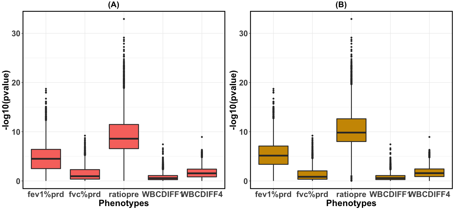
Figure 1:    Boxplot of -log10(P-value) of significant genes for each phenotype. (A) shows the significant genes identified by AFp and (B) shows the significant genes determined by AFz.

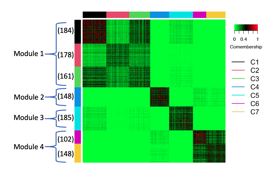
Figure 2: The heatmap of comembership matrix of seven clusters identifed. Red color means two genes are close. The number in the parentheses indicates the sample size of each cluster.

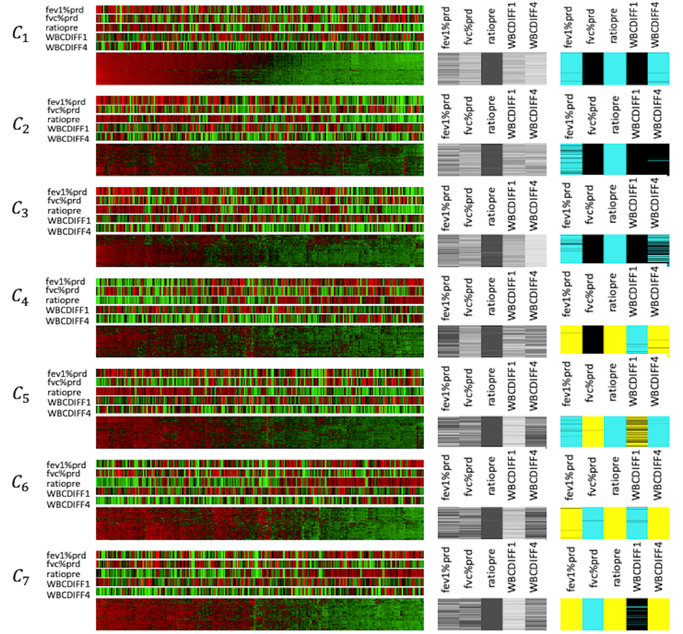
Figure 3: The left panel shows the heatmap of gene expression for each cluster, along with the value of phenotypes for each sample (red color indicates higher expression and green indicates lower expression). The middle panel shows the varibility index of each gene (black indicates low varibility and white indicates high varibility). The right panel shows the weight estimation of each gene (blue represent 1, black represents 0 and yellow represents -1).

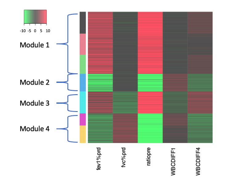
Figure 4: The heatmap shows the $-log_{10}(p_{jk})\times sign(\theta_{jk})$ for $j$th gene and $k$th phenotype among the genes identified in tight clustering. We truncate $-log_{10}(p_{jk})\times sign(\theta_{jk})$ to $[-10,10]$ for better visualization. Green (-10) means a gene is negatively associated with the phenotype and red (10) means a gene is positively associated with the phenotype.

We next conduct pathway enrichment analysis using Fisher’s exact test based on the Gene Ontology (GO), KEGG and Reactome pathway databases to assess the biological relevance of genes and show top 10 significant pathway for each module (Table 6). The top pathways for different modules depict distinct aspects of lung diseases. The top pathways in module 1 involves many DNA damage (Adcock et al., 2018; Sears, 2019) and amino acid alternation/degradation pathways (Engelen and Schols, 2003; Ubhi et al., 2012), which are known to be related to COPD in the literature. Module 2 enriches in many immune response pathways. The immune system needs to react promptly and adequately to potential dangers posed by these microbes and particles, while at the same time avoiding extensive tissue damage and many studies have shown the association between immune response and lung diseases, such as Toll-like receptor and NOD-like receptor (Chaput et al., 2013; Sarir et al., 2008) and kinase-based protein signaling cascades (Mercer and D’Armiento, 2006). Module 3 clearly indicates many extracellular structure pathways which provide structural support and stability to the lung. Changes in the ECM in the airway or parenchymal tissues are now recognized in the pathological profiles of many respiratory diseases including COPD (Burgess et al., 2016). The top pathways in module 4 includes pathways related to cancer and vasculature development. COPD is a risk factor for lung cancer and they have many shared driving factor and genetic effect (Durham and Adcock, 2015). Also, COPD is a risk factor for major cancers developing outside of the lung, including bladder cancer and pancreatic cancer (Divo et al., 2012; Ahn et al., 2020). Furthermore, Angiogenesis (vasculature development) is a shared phenomenon for both cancer and COPD (Matarese and Santulli, 2012), which may indicate the molecular connection between COPD and cancers.

5 Discussion

In this paper, we extend AFp and AFz methods to the scenario of correlated phenotypes based on combinatorial searching for the optimal weight and permutation for determining the significance. Compared with traditional methods targeting at UIT test between each gene and all phenotypes, AFp and AFz can determine the heterogeneity among phenotypes. followed by a bootstrapping algorithm to calculate varibility index and categorize genes. From extensive simulations and the real application, we clearly show that AFp and AFz have robust performance in terms of statistical power under all scenarios. Moreover, AFp has better sensitivity of weight estimation compare with AFz, especially when one phenotype, compared with the others, has much stronger assocation with the gene. AFz tends to assign weight 1 only to the phenotype with strongest association and give weight 0 to all the other phenotypes, which forbids the further gene categorization. In summary, AFp is the method we recommend with superior performance in statistical power, determination of phenotype heterogeneity, gene categorization and biological interpretation by pathway enrichment analysis.

There are three potential limitations in the current study. Firstly, AFp needs permutation to calculate the null distribution and bootstrapping to obtain the comembership matrix for gene categorization which may need heavy computing. To relieve computational burden, we utilize R package “Rfast” (Papadakis et al., 2017) to speed up and also optimize our code to make it in an affordable range for general omics applications. To benchmark computing time, lung disease application ($K=5$, $N=279$ and $p=15,966$) with 50 times bootstrapping using 50 computing threads takes approximately 2 hours to implement AFp method. Secondly, the categorization of genes involves clustering the comembership matrix. Due to the reason that many genes may scatter around and only a small percentage of genes can generate tight clusters, we applied tight clustering algorithm to remove noise genes and generate very tight and striking clusters (Figure 2). However, many other clustering algorithms (hierarchical clustering, $K$-means, self-organizing maps (SOM)) may be worthwhile to try. Thirdly, since AFp uses combinatorial searching for optimal weight, the number of phenotypes should be reasonable. The number of phenotypes is 10 and 5 respectively in simulation and real application parts of this paper and our software can handle this scale well. We would say that in a real application with $5000\sim 20,000$ genes and $200\sim 1000$ samples, usually the number of phenotypes is recommended to be below 10 for computational consideration. Users are suggested to pre-screen phenotypes and only use the phenotypes with biological insight for AFp model.

An R package to implement AFp is available on https://github.com/YujiaLi1994/AFp, along with all data and source code used in this paper.

Table 6:    The pathway enrichment analysis of each module by GO, KEGG and Reactome pathway database. The * sign indicates the P-value is significant under False discovery rate 0.05.

pathway	pvalue
module 1
GO:BP double-strand break repair	4.37e-03
Reactome Double-Strand Break Repair	4.37e-03
KEGG Valine, leucine and isoleucine degradation	6.78e-03
Reactome Branched-chain amino acid catabolism	7.82e-03
Reactome Homologous recombination repair of replication-independent double-strand breaks	1.42e-02
GO:MF phosphotransferase activity, phosphate group as acceptor	1.98e-02
GO:BP gamete generation	2.67e-02
GO:BP sexual reproduction	2.68e-02
GO:MF motor activity	3.39e-02
GO:MF nucleobase-containing compound kinase activity	3.39e-02
module 2
KEGG Toll-like receptor signaling pathway	8.47e-06*
KEGG NOD-like receptor signaling pathway	1.03e-05*
KEGG MAPK signaling pathway	3.91e-05*
GO:BP response to stress	3.95e-05*
KEGG Cytosolic DNA-sensing pathway	4.13e-05*
GO:MF enzyme binding	7.46e-05*
GO:BP protein kinase cascade	8.41e-05*
GO:MF rho gtpase activator activity	8.93e-05*
Reactome NFkB and MAP kinases activation mediated by TLR4 signaling repertoire	1.28e-04*
GO:BP regulation of protein kinase activity	1.55e-04*
module 3
Reactome Extracellular matrix organization	1.48e-08*
Reactome Collagen formation	1.64e-06*
GO:CC proteinaceous extracellular matrix	3.28e-06*
GO:CC extracellular matrix	3.97e-06*
GO:CC extracellular region part	2.66e-05*
GO:CC collagen trimer	7.31e-05*
GO:CC extracellular region	9.26e-05*
GO:CC extracellular matrix component	1.33e-04*
GO:MF glycosaminoglycan binding	3.30e-04
Reactome Diabetes pathways	3.63e-04
module 4
KEGG MAPK signaling pathway	1.87e-04
KEGG Dorso-ventral axis formation	1.89e-04
KEGG Bladder cancer	2.62e-04
KEGG Pancreatic cancer	2.84e-04
GO:MF neurotransmitter binding	3.80e-04
GO:BP angiogenesis	4.28e-04
KEGG Pathways in cancer	4.55e-04
GO:BP organ development	5.51e-04
GO:BP vasculature development	7.34e-04
GO:BP anatomical structure formation involved in morphogenesis	9.83e-04

References

- Adcock et al. (2018) Adcock, I. M., Mumby, S., and Caramori, G. (2018). Breaking news: Dna damage and repair pathways in copd and implications for pathogenesis and treatment.
- Ahn et al. (2020) Ahn, S. V., Lee, E., Park, B., Jung, J. H., Park, J. E., Sheen, S. S., Park, K. J., Hwang, S. C., Park, J. B., Park, H.-S., et al. (2020). Cancer development in patients with copd: a retrospective analysis of the national health insurance service-national sample cohort in korea. BMC pulmonary medicine 20, 1–10.
- Benjamini and Heller (2008) Benjamini, Y. and Heller, R. (2008). Screening for partial conjunction hypotheses. Biometrics 64, 1215–1222.
- Blalock et al. (2004) Blalock, E. M., Geddes, J. W., Chen, K. C., Porter, N. M., Markesbery, W. R., and Landfield, P. W. (2004). Incipient alzheimer’s disease: microarray correlation analyses reveal major transcriptional and tumor suppressor responses. Proceedings of the National Academy of Sciences 101, 2173–2178.
- Burgess et al. (2016) Burgess, J. K., Mauad, T., Tjin, G., Karlsson, J. C., and Westergren-Thorsson, G. (2016). The extracellular matrix–the under-recognized element in lung disease? The Journal of pathology 240, 397–409.
- Chaput et al. (2013) Chaput, C., Sander, L. E., Suttorp, N., and Opitz, B. (2013). Nod-like receptors in lung diseases. Frontiers in immunology 4, 393.
- Divo et al. (2012) Divo, M., Cote, C., de Torres, J. P., Casanova, C., Marin, J. M., Pinto-Plata, V., Zulueta, J., Cabrera, C., Zagaceta, J., Hunninghake, G., et al. (2012). Comorbidities and risk of mortality in patients with chronic obstructive pulmonary disease. American journal of respiratory and critical care medicine 186, 155–161.
- Durham and Adcock (2015) Durham, A. and Adcock, I. (2015). The relationship between copd and lung cancer. Lung Cancer 90, 121–127.
- Engelen and Schols (2003) Engelen, M. P. and Schols, A. M. (2003). Altered amino acid metabolism in chronic obstructive pulmonary disease: new therapeutic perspective? Current Opinion in Clinical Nutrition & Metabolic Care 6, 73–78.
- Fisher (1992) Fisher, R. A. (1992). Statistical methods for research workers. In Breakthroughs in statistics, pages 66–70. Springer.
- Huo et al. (2020) Huo, Z., Tang, S., Park, Y., and Tseng, G. (2020). P-value evaluation, variability index and biomarker categorization for adaptively weighted fisher?s meta-analysis method in omics applications. Bioinformatics 36, 524–532.
- Matarese and Santulli (2012) Matarese, A. and Santulli, G. (2012). Angiogenesis in chronic obstructive pulmonary disease: a translational appraisal. Translational Medicine@ UniSa 3, 49.
- Mercer and D’Armiento (2006) Mercer, B. A. and D’Armiento, J. M. (2006). Emerging role of map kinase pathways as therapeutic targets in copd. International journal of chronic obstructive pulmonary disease 1, 137.
- O’Brien (1984) O’Brien, P. C. (1984). Procedures for comparing samples with multiple endpoints. Biometrics pages 1079–1087.
- O’Reilly et al. (2012) O’Reilly, P. F., Hoggart, C. J., Pomyen, Y., Calboli, F. C., Elliott, P., Jarvelin, M.-R., and Coin, L. J. (2012). Multiphen: joint model of multiple phenotypes can increase discovery in gwas. PloS one 7, e34861.
- Pan et al. (2014) Pan, W., Kim, J., Zhang, Y., Shen, X., and Wei, P. (2014). A powerful and adaptive association test for rare variants. Genetics 197, 1081–1095.
- Papadakis et al. (2017) Papadakis, M., Tsagris, M., Dimitriadis, M., Fafalios, S., Papadakis, M. M., Rcpp, L., and LazyData, T. (2017). Package ‘rfast’.
- Peters et al. (2015) Peters, M. J., Joehanes, R., Pilling, L. C., Schurmann, C., Conneely, K. N., Powell, J., Reinmaa, E., Sutphin, G. L., Zhernakova, A., Schramm, K., et al. (2015). The transcriptional landscape of age in human peripheral blood. Nature communications 6, 1–14.
- Potter (2005) Potter, D. M. (2005). A permutation test for inference in logistic regression with small-and moderate-sized data sets. Statistics in medicine 24, 693–708.
- Ritchie et al. (2015) Ritchie, M. E., Phipson, B., Wu, D., Hu, Y., Law, C. W., Shi, W., and Smyth, G. K. (2015). limma powers differential expression analyses for rna-sequencing and microarray studies. Nucleic acids research 43, e47–e47.
- Robinson et al. (2010) Robinson, M. D., McCarthy, D. J., and Smyth, G. K. (2010). edger: a bioconductor package for differential expression analysis of digital gene expression data. Bioinformatics 26, 139–140.
- Roy (1953) Roy, S. N. (1953). On a heuristic method of test construction and its use in multivariate analysis. The Annals of Mathematical Statistics pages 220–238.
- Sarir et al. (2008) Sarir, H., Henricks, P. A., van Houwelingen, A. H., Nijkamp, F. P., and Folkerts, G. (2008). Cells, mediators and toll-like receptors in copd. European journal of pharmacology 585, 346–353.
- Sears (2019) Sears, C. R. (2019). Dna repair as an emerging target for copd-lung cancer overlap. Respiratory investigation 57, 111–121.
- Song et al. (2016) Song, C., Min, X., and Zhang, H. (2016). The screening and ranking algorithm for change-points detection in multiple samples. The annals of applied statistics 10, 2102.
- Tippett et al. (1931) Tippett, L. H. C. et al. (1931). The methods of statistics. The Methods of Statistics. .
- Tseng and Wong (2005) Tseng, G. C. and Wong, W. H. (2005). Tight clustering: A resampling-based approach for identifying stable and tight patterns in data. Biometrics 61, 10–16.
- Ubhi et al. (2012) Ubhi, B. K., Cheng, K. K., Dong, J., Janowitz, T., Jodrell, D., Tal-Singer, R., MacNee, W., Lomas, D. A., Riley, J. H., Griffin, J. L., et al. (2012). Targeted metabolomics identifies perturbations in amino acid metabolism that sub-classify patients with copd. Molecular BioSystems 8, 3125–3133.
- Van der Sluis et al. (2013) Van der Sluis, S., Posthuma, D., and Dolan, C. V. (2013). Tates: efficient multivariate genotype-phenotype analysis for genome-wide association studies. PLoS Genet 9, e1003235.
- Werft and Benner (2010) Werft, W. and Benner, A. (2010). glmperm: A permutation of regressor residuals test for inference in generalized linear models. The R Journal 2, 39–43.
- Wu and Pankow (2016) Wu, B. and Pankow, J. S. (2016). Sequence kernel association test of multiple continuous phenotypes. Genetic epidemiology 40, 91–100.
- Zhang et al. (2014) Zhang, Y., Xu, Z., Shen, X., Pan, W., Initiative, A. D. N., et al. (2014). Testing for association with multiple traits in generalized estimation equations, with application to neuroimaging data. NeuroImage 96, 309–325.