Symmetries of the nucleon-nucleon $S$-matrix
and effective field theory expansions

Abstract

The s-wave nucleon-nucleon (NN) scattering matrix ($S$-matrix) exhibits UV/IR symmetries which are hidden in the effective field theory (EFT) action and scattering amplitudes, and which explain some generic features of the phase shifts. These symmetries offer clarifying interpretations of existing pionless EFT expansions, and suggest starting points for novel expansions. The leading-order (LO) $S$-matrix obtained in the pionless EFT with scattering lengths treated exactly is shown to have a UV/IR symmetry which leaves the sum of s-wave phase shifts invariant. A new scheme, which treats effective range corrections exactly, and which possesses a distinct UV/IR symmetry at LO, is developed up to NLO (next-to-LO) and compared with data.

1 Introduction

The language of EFT was commonplace among particle physics graduate students in the late 80’s and early 90’s. The syntax of this language is quite simple and intuitive and amounts primarily to counting dimensions of operators, and, for quantitative calculations, including quantum effects perturbatively, as in the canonical example of the chiral perturbation theory expansion Weinberg:1978kz ; Gasser:1983yg . This use of EFT requires an understanding of regularization and renormalization at the level of the textbook treatment of $\lambda\phi^{4}$ theory. Indeed, this was covered in detail in Weinberg’s two-year quantum field theory sequence (attended by one of the authors) that took place several times in that era and just preceded the initial publication of his classic textbooks.

Contemporaneously, Weinberg’s papers on EFT for nuclear physics provided an organizational principle —based in QCD and its symmetries— for establishing the most important terms in the nuclear potential Weinberg:1990rz ; Weinberg:1991um ; Weinberg:1992yk . However there was not much mention in these papers of the manner in which the highly singular potentials would be regulated and renormalized, or how such a procedure would modify the organizational principle. The initial papers applying Weinberg’s ideas focused primarily on a direct numerical evaluation of phase shifts to several non-trivial orders in the expansion and largely ignored issues of renormalization by smoothing out singular contributions to the potential using effective form factors Ordonez:1992xp ; Ordonez:1993tn ; Ordonez:1995rz , the standard practice in the nuclear physics community at the time. Eventually, the issue of renormalization in Weinberg’s scheme was carefully considered in simple cases and rather dramatic inconsistencies were found in the potentials describing the simplest NN scattering phase shifts, initially in the s-wave channels Kaplan:1996xu , and later in the p-wave channels Nogga:2005hy . These observation spawned a research program into the internal consistency of Weinberg’s program which has lasted over two decades and which still has achieved no consensus. In parallel with this rather abstract theoretical research program, the nuclear physics community has increasingly adopted the initial Weinberg paradigm, while sometimes providing apologias for the original renormalization issues; see, e.g. Epelbaum:2008ga ; Machleidt:2011zz . Indeed, one could argue that, while Weinberg’s program has been pushed to ever increasing sophistication and to larger and more complex nuclear systems, the initial formal issues with consistent renormalization —for the most fundamental systems (i.e. NN and NNN) which are foundational to the entire program— remain unresolved.

All of the above is in reference to the EFT relevant for characteristic momenta $k\sim M_{\pi}$ and which therefore includes the pion as a propagating degree of freedom in the EFT Lagrangian. Pions introduce the complexities of a highly-singular tensor force, as well as non-trivial aspects of the chiral symmetry of QCD. Efforts to resolve the renormalization issues with Weinberg’s program led to a new EFT proposal in which pions are treated in perturbation theory and consistent renormalization is manifest Kaplan:1998tg ; Kaplan:1998we . While this scheme ultimately failed to agree with the real world Fleming:1999ee , it was an important success as regards the change of mindset in nuclear physics that was brought by Weinberg’s work: it clearly demonstrated that a specific EFT organizational principle, such as the one proposed in Ref. Kaplan:1998tg ; Kaplan:1998we , is falsifiable.

By contrast, inspired by Weinberg’s work, tremendous progress was made in understanding renormalization for $k\sim 1/a_{s}\ll M_{\pi}$, where $a_{s}$ ($s=0,1$) are the s-wave NN scattering lengths vanKolck:1998bw ; Kaplan:1998tg ; Kaplan:1998we ; Birse:1998dk . At these distance scales the pion and all its complexities can happily be integrated out, leaving a relatively simple EFT with nucleon degrees of freedom, generally interacting with some external currents. In the initial studies of EFTs of NN scattering in which the potential is treated exactly, a fundamental point of confusion lay in the belief that NN scattering could be described by a coordinate-space potential given by a gradient expansion of delta-function interactions. That this is not the case was shown explicitly in Ref. Beane:1997pk , based on earlier work which had clarified Wigner’s causality bounds on scattering parameters in the language of EFT Phillips:1996ae ; Scaldeferri:1996nx ; Phillips:1997xu ; Hammer:2010fw . Long ago Wigner showed that causality places constraints on scattering parameters in quantum mechanical scattering with potentials of finite range Wigner:1955zz . In the EFT paradigm, in mass-dependent schemes like cutoff regularization, the UV momentum-space cutoff acts like the inverse of the range of interaction. While this relation is somewhat fuzzy, removal of the cutoff in the renormalization procedure is operationally equivalent to taking the range of interaction to zero.

It is worth mentioning here the flawed analogy between a non-perturbative cutoff EFT of nuclear physics and EFTs of QCD relevant for lattice QCD simulations. While there is a clear parallel between the lattice QCD action with Symanzik improvement and the nuclear EFT Lagrangian, lattice QCD has a continuum limit which is consistent with all general physical principles, including causality while causality —via the Wigner bound— prohibits nuclear EFT from achieving a continuum limit. This is no surprise physically: both nuclear EFT and lattice QCD formally find their UV completion in QCD. However, nucleonic degrees of freedom lose their meaning in the approach to the continuum limit, and this is, at least qualitatively, reflected in the Wigner bound in NN scattering. In some sense, the Wigner bound pigeonholes nuclear EFT into the Wilsonian paradigm where a cutoff on short-distance modes is implemented and then varied over some range in order to demonstrate cutoff independence order-by-order in the EFT.

The Wigner bound applies only when a strictly finite-range potential is treated exactly, giving rise to a unitary $S$-matrix. Treating the NN s-wave effective-range parameters to be of order the range of interaction of the potential, allows the gradients of delta-function potentials to be treated in perturbation theory vanKolck:1998bw ; Kaplan:1998tg ; Kaplan:1998we ; Birse:1998dk , and this renders the Wigner bounds a non-issue. A highly efficient pionless EFT, in which non-perturbative nuclear binding arises from treating the momentum-independent four-nucleon operators exactly, while momentum-dependent operators are treated in perturbation theory, has proven to be a remarkably successful paradigm for low-energy few-body interactions with large scattering lengths vanKolck:1998bw ; Kaplan:1998tg ; Kaplan:1998we ; Chen:1999tn ; Hammer:2019poc . Of course, the inherent ambiguity in the form of the nuclear EFT potential at short distance allows avoidance of the Wigner bound even when the potential —including momentum-dependent operators— is treated exactly Gegelia:1998gn , as long as the range of the interaction is kept finite. However, as will be seen below, in this case it is challenging to express amplitudes in a useful form, as renormalization conditions have to be imposed at all orders in the momentum expansion.

As the s-wave NN effective ranges are somewhat large as compared to the pion’s Compton wavelength, and indeed the pionless EFT expansion is rendered more effective by expanding about the deuteron or dibaryon pole which subsumes effective range corrections Phillips:1999hh ; Gegelia:2001ev ; SanchezSanchez:2017tws , it makes sense to treat the range-corrections exactly Kaplan:1999qa while continuing to treat shape-parameter effects in perturbation theory. A practical way to achieve this is by making use of the dibaryon scheme developed for NN scattering in Ref. Kaplan:1996nv and formulated in detail, with many examples, in Ref. Beane:2000fi . This method effectively includes range corrections non-perturbatively through the use of energy-dependent potentials which, from the EFT perspective, can be constructed using operator ambiguities and the freedom of field redefinition. One of the goals of this contribution is to provide an EFT scheme which treats effective-range corrections exactly using energy-independent interactions. It may come as a surprise that there is a powerful symmetry which constrains this system, and facilitates the avoidance of the Wigner bound in a useful manner.

In the Wilsonian paradigm, EFTs are viewed as perturbations about fixed points of the renormalization group (RG) Birse:1998dk . In non-relativistic s-wave scattering with finite-range forces, the running couplings exhibit two interesting fixed points, the trivial fixed point where there is no interaction, and the unitary fixed point where the interaction is as strong as it can be without violating unitarity. At both fixed points, the EFT exhibits conformal invariance or Schrödinger symmetry Mehen:1999nd . Note however that the notion that EFTs of contact forces are expansions about fixed points of the RG is not strictly-speaking correct, as, at the fixed point itself, there is no scattering. That is, the LO amplitude, with finite scattering lengths, has an intrinsic scale and is therefore in itself necessarily a perturbation about the RG fixed point.

The main point that will be conveyed in this contribution is that the simplest $S$-matrices which describe s-wave scattering with finite-range forces near (but not at) unitarity exhibit exact UV/IR symmetries Beane:2020wjl ; Beane:2021bpr ; Beane:2021xrk . A new viewpoint here that may be unfamiliar to the reader is the focus on the symmetries of the $S$-matrix, rather than the symmetries of the action or the scattering amplitude. In addition to providing a new way of viewing the EFT near the unitary fixed point, UV/IR symmetries suggest novel EFT expansions. In particular, the s-wave scattering system at low energies, with scattering length and effective range corrections treated exactly, is considered in detail as an example of the power and utility of the UV/IR symmetries.

2 The $S$-matrix and UV/IR symmetry

Below inelastic thresholds, the unitary s-wave scattering amplitude for a finite range potential is given by the effective range expansion (ERE)

$$T(k)\ =\ -\frac{4\pi}{M}\left[-\frac{1}{a}+\frac{1}{2}r{k^{2}}+v_{2}k^{4}+v_{3}k^{6}+O(k^{8})-ik\right]^{-1},$$ (1)

where $k=\sqrt{ME}$ is the on-shell center-of-mass (c.o.m.) momentum, $a$ is the scattering length, $r$ is the effective range, and the $v_{i}$ are shape parameters. With the normalization of the scattering amplitude implied by Eq. (1), the $S$-matrix element is given by

$$S\ =\ e^{2i\delta(k)}\ =\ 1\ -\ i\frac{kM}{2\pi}T(k)\ .$$ (2)

Consider the scattering length approximation, where all effective range and shape parameters are taken to vanish. In this case, the scattering amplitude and $S$-matrix element are

$$T(k)\ =\ \frac{4\pi}{M}\frac{a}{1+iak}\ \ \ ,\ \ \ S(k)\ =\ \frac{1-iak}{1+iak}\ .$$ (3)

It is immediately clear that $S$ has a symmetry which is not a symmetry of $T$. The scale transformation $k\mapsto e^{\beta}k$, $a\mapsto e^{-\beta}a$ leaves $S$ invariant and simply implies that varying $k$ with $a$ fixed is the same as varying $a$ with $k$ fixed. The trivial fixed point, $S=1$, is reached with no interaction, $a=0$ or with $k=0$, and the unitary fixed point, $S=-1$, is reached with $a$ infinite or with $k$ infinite.

Now consider the momentum inversion

$$k\mapsto{1\over a^{2}k}\ .$$ (4)

The transformation on $T$ is complicated, however, it implies a simple transformation of the $S$-matrix element

$$\delta(k)\mapsto-\delta(k)\pm\frac{\pi}{2}\ \ \ \ S\to-S^{*}\ ,$$ , (5)

where the sign of the $\pi/2$ phase is determined by the sign of the scattering length. This momentum inversion clearly interchanges the trivial and unitary RG fixed points. As the trivial RG fixed point is, by definition, not seen by the scattering amplitude, it is no surprise that the momentum inversion symmetry does not act simply on $T$. The transformation interrelates the scattering amplitude and the unit operator, and thus is realized on the $S$-matrix.

It may seem that the momentum inversion transformation of Eq. (4) is orthogonal to the idea of EFT since it interchanges the UV and the IR. Note however that at LO in the EFT, one is considering scattering in a limit in which all short-distance mass scales are taken to be very large. In this limit, long-distance forces (like pion exchange) and inelastic thresholds (like the pion-production threshold) are only probed as momentum approaches infinity. Therefore it is reasonable, at LO, to consider transformations of the momenta over the entire momentum half-line, $0<k<\infty$.

The fixed point of the momentum-inversion transformation is the momentum that maps into itself under inversion, $k^{\circ}=|a|^{-1}$, which is the absolute value of the scattering amplitude’s pole position in the complex momentum plane. Therefore the EFT which reproduces the scattering length approximation is, strictly speaking, an expansion about the fixed point, $k^{\circ}$, of the UV/IR transformation.

Next, consider the inclusion of effective range effects with shape parameters taken to vanish. In this case, the momentum inversion

$$k\mapsto{2\over|ar|k}\ ,$$ (6)

implies the transformations of the $S$-matrix element

$$\delta(k)\mapsto-\delta(k)\ \ \ \ S\to S^{*}\ \ ,\ \ ar>0\ ,$$ ,

$$\delta(k)\mapsto\delta(k)\ \ \ \ S\to S\ \ ,\ \ ar<0\ .$$ , (7)

The absence of a phase in this transformation reflects that, as a function of momentum, the $S$-matrix element begins and ends at the trivial RG fixed point, $S=1$. This momentum inversion has the fixed point $k^{\circ}=\sqrt{2}|ar|^{-1/2}$, which is the square root of the absolute value of the product of the scattering amplitude’s two pole positions in the complex momentum plane. Again, if this amplitude with vanishing shape parameters is treated as LO in an EFT, then the expansion is about the scale set by this fixed point.

3 UV/IR symmetries of the NN s-wave $S$-matrix

Realistic NN scattering at low energies is not a single-channel system as the initial-state nucleons can be arranged into two distinct spin configurations. The NN $S$-matrix at very low energies is dominated by the s-wave and can be written as Beane:2018oxh ; Beane:2020wjl

$$\hat{\bf S}(\delta_{0},\delta_{1}) = {1\over 2}\left(S_{1}+S_{0}\right)\hat{\bf 1}\ +\ {1\over 2}\left(S_{1}-S_{0}\right){\cal P}_{12}\ ,$$ (8)

where now

$$S_{s}\ =\ e^{2i\delta_{s}(k)}\ ,$$ (9)

the SWAP operator is

$${\cal P}_{12}=\textstyle{1\over 2}\left({\hat{\bf 1}}+\hat{\bm{\sigma}}\cdot\hat{\bm{\sigma}}\right)$$ (10)

and, in the direct-product space of the nucleon spins,

$$\hat{\bf 1}\equiv\hat{\cal I}_{2}\otimes\hat{\cal I}_{2}\ \ \ ,\ \ \hat{\bm{\sigma}}\cdot\hat{\bm{\sigma}}\equiv\sum\limits_{\alpha=1}^{3}\ \hat{\sigma}^{\alpha}\otimes\hat{\sigma}^{\alpha}\ ,$$ (11)

with ${\cal I}_{2}$ the $2\times 2$ unit matrix, and $\hat{\sigma}^{\alpha}$ the Pauli matrices. The $\delta_{s}$ are s-wave phase shifts with $s=0$ corresponding to the spin-singlet (${}^{1}\hskip-2.168ptS_{0}$) channel and $s=1$ corresponding to the spin-triplet (${}^{3}\hskip-1.8063ptS_{1}$) channel. Below, the following physical effective range parameters will be used Kaplan:1998we ; deSwart:1995ui : $a_{0}=-23.714(13)$ fm, $a_{1}=5.425(1)$ fm, $r_{0}=2.73(3)$ fm, and $r_{1}=1.749(8)$ fm.

The momentum-inversion transformations of the $S$-matrix elements considered above are not transformations that act simply on the full $S$-matrix as they are s-wave channel dependent. However, these transformations can be readily generalized to the full $S$-matrix. In the scattering length approximation, consider the momentum inversion transformation Beane:2020wjl

$$p\mapsto\frac{1}{|a_{1}a_{0}|p}\ .$$ (12)

This implies the following transformations on the phase shifts for the NN physical case $a_{1}a_{0}<0$:

$$\delta_{0}(p)\mapsto\delta_{1}(p)-\frac{\pi}{2}\ \ \ ,\ \ \ \ \ \,\delta_{1}(p)\mapsto\delta_{0}(p)+\frac{\pi}{2}\ .$$ (13)

This transformation therefore corresponds to an exact symmetry, which leaves the combination of phase shifts $\delta_{0}+\delta_{1}$ invariant. As phase shifts are angles, this is, by definition, a conformal invariance, albeit one that allows the presence of a mass scale. This conformal invariance facilitates the construction of a purely geometrical theory of scattering Beane:2020wjl ; Beane:2021bpr .

With effective range corrections included, the momentum inversion transformation

$$p\mapsto\frac{1}{\lambda|a_{1}a_{0}|p}\ ,$$ (14)

with the arbitrary real parameter $\lambda>0$, implies

$$\delta_{0}(p)\mapsto\delta_{0}(p)\ \ \ ,\ \ \ \ \ \,\delta_{1}(p)\mapsto-\delta_{1}(p)\ ,$$ (15)

but only in the special case where the effective ranges are correlated with the scattering lengths as

$$r_{0} = 2\lambda a_{1}\ \ \ ,\ \ \ r_{1}\,=\,-2\lambda a_{0}\ .$$ (16)

This UV/IR symmetry has interesting implications for nuclear physics. The measured singlet NN scattering phase shift rises steeply from zero due to the unnaturally large scattering length, and then, as momenta approach inelastic threshold, the phase shift goes through zero and becomes negative, indicating the fabled short-distance repulsive core. While this impressionistic description assigns physics to the potential, which is not an observable and indeed need not be repulsive at short distances, the UV/IR symmetry directly imposes the physically observed behavior of the phase shift. Even though the singlet phase shift changes sign at momenta well beyond the range of applicability of the pionless theory, ascribing this symmetry to the LO results —through the required presence of range corrections— results in a more accurate LO prediction than the usual pionless expansion SanchezSanchez:2017tws .

4 EFT description: single-channel case

4.1 Potential and Lippmann-Schwinger equation

It is convenient to introduce the generic UV scale ${\cal M}$ and the generic IR scale $\aleph$. The EFT will describe physics for $k\sim\aleph\ll{\cal M}$. Subleading corrections to the scattering amplitude in the EFT are expected to be parametrically suppressed by powers of $k/{\cal M}$. For the NN system at very-low energies, described by the pionless EFT, the UV scale is ${\cal M}\sim M_{\pi}$.

The s-wave potential stripped from the most general effective Lagrangian of four-nucleon contact operators is Kaplan:1996nv ; Phillips:1997xu

$$V(p^{\prime},p)=C_{0}+C_{2}\left(p^{2}+p^{\prime 2}\right)+C_{4}\left(p^{4}+p^{\prime 4}\right)+C_{4}^{\prime}p^{2}p^{\prime 2}+\dots\ ,$$ (17)

where the $C_{n}$ are the bare coefficients. The scattering amplitude is obtained by solving the Lippmann-Schwinger (LS) equation with this potential

$$T(p^{\prime},p;E)=V(p^{\prime},p)+M\int\frac{d^{3}q}{(2\pi)^{3}}\,V(p^{\prime},q)\frac{1}{EM-{q^{2}}+i\epsilon}T(q,p;E)\ .$$ (18)

As the potential is separable to any order in the momentum expansion, the scattering amplitude can be obtained in closed form to any desired order in the potential Phillips:1997xu . Of course the singular nature of the potential requires regularization and renormalization. The scattering amplitude can be regulated using, for instance, dimensional regularization and its various schemes, or by simply imposing a hard UV cutoff, $\Lambda$, on the momentum integrals.

4.2 Matching equations

In the language of cutoff regularization, matching the solution of the LS equation with the ERE of Eq. (1), formally gives the all-orders matching equations

$$a = f_{0}(\Lambda;C_{0},C_{2},C_{4},\ldots)\ ,$$

$$r = f_{2}(\Lambda;C_{0},C_{2},C_{4},\ldots)\ ,$$

$$v_{n} = f_{2n}(\Lambda;C_{0},C_{2},C_{4},\ldots)\ ,$$ (19)

where the $f_{2n}$ are non-linear functions determined by solving the LS equation. These equations can be inverted to find the now cutoff-dependent coefficients $C_{2n}(\Lambda;a,r,v_{2},\ldots)$. To obtain an EFT with predictive power, it is necessary to identify the relative size of the effective range parameters. If they all scale as powers of ${\cal M}^{-1}$, then the entire potential of Eq. (17) can be treated in perturbation theory for momenta $k\ll{\cal M}$. If there are big parts that instead scale as powers of ${\aleph}^{-1}$, they will, via the interactions of Eq. (17), constitute the LO potential in the EFT expansion.

4.3 Scattering length approximation

With $a\sim\aleph^{-1}$ and the effective range and shape parameters of natural size, $r\sim{\cal M}^{-1}$, $v_{n}\sim{\cal M}^{-2n+1}$, the amplitude can be expanded for $k\ll{\cal M}$ as

$$T(k)\ =\ -\frac{4\pi}{M}\left(-\frac{1}{a}-ik\right)^{-1}\bigg{[}1+O(k)\bigg{]}\ .$$ (20)

In order to generate this expansion in the EFT, the potential is written as

$$V(p^{\prime},p)=V_{\scriptscriptstyle{LO}}+V_{r}(p^{\prime},p)\ ,$$ (21)

where $V_{\scriptscriptstyle{LO}}=C_{0}$ is treated exactly in the LS equation and the residual potential, $V_{r}$, which includes range and shape parameter corrections, is treated in perturbation theory. Keeping the first term in the s-wave potential, the solution of the LS equation is

$$T_{\scriptscriptstyle{LO}}(k)=\left(\frac{1}{C_{0}}-{\mathbb{I}}(k)\right)^{-1},$$ (22)

where

$$\mathbb{I}(k)\equiv\left(\frac{\omega}{2}\right)^{3-d}M\int\frac{d^{d}q}{(2\pi)^{d}}\,\frac{1}{{k^{2}}-{q^{2}}+i\epsilon}\ \ {\smash{\mathop{{\relbar\joinrel\longrightarrow}}\limits^{\rm PDS}}}\ \ -\frac{M}{4\pi}\left(\omega+ik\right)\ ,$$ (23)

has been evaluated in dimensional regularization with the PDS scheme Kaplan:1998tg ; Kaplan:1998we and renormalized at the RG scale $\omega$. The matching equations in this case are

$$a=\left(\frac{4\pi}{MC_{0}}+\omega\right)^{-1}\ ,$$

$$r=v_{n}=0\ .$$ (24)

Inverting one finds

$$C_{0}(\omega)\ =\ \frac{4\pi}{M}\frac{1}{{1}/{a}-{\omega}}\ .$$ (25)

The coupling at the unitary fixed point, $C_{0}=C_{0\star}$, corresponds to a divergent scattering length (unitarity). A rescaled coupling can be defined as ${\hat{C}}_{0}\equiv C_{0}/C_{0\star}$. The corresponding beta-function is then

$${\hat{\beta}({\hat{C}}_{0})}\ =\ \omega\frac{d}{d\omega}{\hat{C}}_{0}(\omega)\ =\ -{\hat{C}}_{0}(\omega)\left({\hat{C}}_{0}(\omega)-1\right)\ ,$$ (26)

which explicitly has fixed points at ${\hat{C}}_{0}=0$ and $1$. Now note that the beta-function is invariant with respect to the inversion of the RG scale Beane:2021xrk

$$\omega\mapsto{1\over a^{2}\omega}\ ,$$ (27)

which interchanges the trivial and unitary fixed points

$${\hat{C}}_{0}(\omega)\leftrightarrow 1-{\hat{C}}_{0}(\omega)\ .$$ (28)

This exactly mirrors the action of the UV/IR transformation on the $S$-matrix elements as was shown in section 2, and shares the fixed point $\omega^{\circ}=k^{\circ}=|a|^{-1}$. The moral here is that while the UV/IR transformation is not simply realized at the level of the EFT action, its effect is manifest in the RG flow of the EFT operators Beane:2021xrk .

4.4 Range corrections with zero-range forces

With $a,r\sim\aleph^{-1}$ and shape parameters of natural size, $v_{n}\sim{\cal M}^{-2n+1}$, the amplitude can be expanded for $k\ll{\cal M}$ as

$$T(k)\ =\ -\frac{4\pi}{M}\left(-\frac{1}{a}+\frac{1}{2}r{k^{2}}-ik\right)^{-1}\bigg{[}1+O(k^{3})\bigg{]}\ .$$ (29)

In order to generate this expansion from the EFT perspective, one may choose $V_{\scriptscriptstyle{LO}}=C_{0}+C_{2}\left(p^{2}+p^{\prime 2}\right)$. Due to the highly singular UV behavior of this potential, cutoff regularization will be used to carefully account for the divergences that are generated when solving the LS equation. The amplitude is found in closed form to be Phillips:1997xu

$$T_{\scriptscriptstyle{LO}}(k)=\left(\frac{(C_{2}I_{3}-1)^{2}}{C+C_{2}^{2}I_{5}+{k^{2}}C_{2}(2-C_{2}I_{3})}-{\mathbb{I}}(k)\right)^{-1}\ ,$$ (30)

where now ${\mathbb{I}}(k)$ is evaluated with cutoff regularization, and

$$I_{n}\equiv-M\int\frac{d^{3}q}{(2\pi)^{3}}q^{n-3}\theta\left(\frac{\pi}{2}\Lambda-q\right)=-\frac{M\Lambda^{n}}{2^{1+n}\pi^{2-n}n}\ .$$ (31)

Matching the amplitude to the ERE gives

$$a = \frac{M}{4\pi}\left(\frac{(C_{2}I_{3}-1)^{2}}{C+C_{2}^{2}I_{5}}-{I_{1}}\right)^{-1}\ ,$$

$$r = \frac{8\pi}{M}\left(\frac{(C_{2}I_{3}-1)^{2}}{C+C_{2}^{2}I_{5}}\right)^{2}\left[\frac{1}{(C_{2}I_{3}-1)^{2}I_{3}}-\frac{1}{I_{3}}\right]\ ,$$

$$v_{n} = -\frac{4\pi}{M}\frac{C_{2}^{n}(C_{2}I_{3}-2)^{n}(C_{2}I_{3}-1)^{2}}{(C+C_{2}^{2}I_{5})^{n+1}}\ .$$ (32)

Taking the limit $\Lambda\rightarrow\infty$ then recovers the ERE with all shape parameter corrections vanishing, $v_{n}=0$. However, it is straightforward to verify that in this limit, $r\leq 0$, as required by the Wigner bound Wigner:1955zz . If s-wave NN scattering involved negative effective ranges and resonances rather than bound states, then this scheme, with the effective potential consisting of a finite number of strictly delta-function potentials, would suffice Habashi:2020qgw . However, as the s-wave NN effective ranges are both positive, it is clear that $\Lambda$ must be kept finite. In that case the higher-order terms in the bare potential, even if neglected in the choice of $V_{\scriptscriptstyle{LO}}$, are generated quantum mechanically at LO as evidenced by the non-vanishing shape parameters. Therefore the higher order operators should be kept from the start. That is, one is back to the general, formal statement of the matching conditions given in Eq. (19), where a renormalization scheme is required which ensures that $v_{n}=0$, and a choice of $V_{\scriptscriptstyle{LO}}$ must be found which achieves this while including all orders in the momentum expansion.

4.5 Range corrections with a finite-range scheme: LO

The lesson provided by the Wigner bound is that if range corrections are treated exactly, then the LO potential should, in general, include all orders in the momentum expansion. Therefore, the potential can be written as in Eq. (21) except now with a momentum dependent LO potential

$$V(p^{\prime},p)=V_{\scriptscriptstyle{LO}}(p^{\prime},p)+V_{r}(p^{\prime},p)\ .$$ (33)

The residual potential, $V_{r}$, which accounts for NLO and higher effects in perturbation theory, will be considered in detail below. Now the potential is non-unique and there is no reason for the separation into $V_{\scriptscriptstyle{LO}}$ and $V_{r}$ to be unique. Ideally one finds a LO potential which identically gives the ERE with all shape parameters vanishing, and indeed that is what will be achieved by imposing the UV/IR symmetry at the level of the interaction.

As the s-wave EFT potential is non-local (non-diagonal in coordinate space) and separable to any order in the momentum expansion, it appears sensible to assume that the LO potential which generates the ERE with range corrections only is non-local and separable. However, such an assumption is not necessary: all potentials which generate the ERE truncated at the effective range are, by definition, phase equivalent. Once one potential is found, others can be obtained by unitary transformation. Here the simplest possibility will be considered; that the LO potential is (rank-one) separable.

For a separable potential $V(p,p^{\prime})$, the on-shell scattering amplitude solves the LS equation algebraically to

$$T(k)\ =\ {V(k,k)}\left(1-M\int\frac{d^{3}q}{(2\pi)^{3}}\,\frac{V(q,q)}{{k^{2}}-{q^{2}}+i\epsilon}\right)^{-1}\ .$$ (34)

The momentum inversion symmetry of Eq. (6) (assuming for simplicity $\eta\equiv ar/2>0$) implies

$$T(k)\mapsto T\left({1\over{\eta k}}\right)\ =\ -\eta k^{2}\,T^{*}(k)\ .$$ (35)

With the range of the potential taken to be the momentum scale $\mu$, the potential can be taken to be the real function $V_{\scriptscriptstyle{LO}}(\mu;p,p^{\prime})$. Constraints on the $S$-matrix concern the potential $V_{\scriptscriptstyle{LO}}(\mu;p,p)\equiv V_{\scriptscriptstyle{LO}}(\mu;p)$. Therefore,

$$T^{*}(k) = {V_{\scriptscriptstyle{LO}}\left(\mu;k\right)}\left({1-M\int\frac{d^{3}q}{(2\pi)^{3}}\,\frac{V_{\scriptscriptstyle{LO}}(\mu;q)}{{k^{2}}-{q^{2}}-i\epsilon}}\right)^{-1}$$ (36)

$$= \frac{-\frac{1}{\eta k^{2}}V_{\scriptscriptstyle{LO}}\left(\mu;{1\over{\eta k}}\right)}{\bigg{[}1-\frac{M}{2\pi^{2}}\int dq\,\left(-\frac{1}{\eta q^{2}}\right){V_{\scriptscriptstyle{LO}}(\mu;{1\over{\eta q}})}\bigg{]}-M\int\frac{d^{3}q}{(2\pi)^{3}}\,\left(-\frac{1}{\eta q^{2}}\right)\frac{V_{\scriptscriptstyle{LO}}(\mu;{1\over{\eta q}})}{{k^{2}}-{q^{2}}-i\epsilon}}$$

where the first line follows from Eq. (34) and the second line follows from Eq. (35). Now consider non-singular solutions of this equation of the form

$$V_{\scriptscriptstyle{LO}}\left(\mu;{1\over{\eta q}}\right)\ =\ \epsilon\,\eta q^{2}\;V_{\scriptscriptstyle{LO}}(\nu;q)\ ,$$ (37)

where $\epsilon=\pm 1$, and the range of the potential has been allowed to vary under momentum inversion, and so $\nu$ is an independent scale in correspondence with the range of the transformed potential. Integrating this equation gives

$$\int_{0}^{\infty}dq\,V_{\scriptscriptstyle{LO}}\left(\mu;q\right)\ =\ \epsilon\,\int_{0}^{\infty}dq\,V_{\scriptscriptstyle{LO}}(\nu;q)\ .$$ (38)

With the choice $\epsilon=-1$ and $\mu=\nu$, this integral must vanish identically and there is clearly a formal solution to Eq. (36). However, an explicit solution does not seem to exist for a real, finite-range potential.

What follows focuses on the case $\epsilon=1$ and $\mu\neq\nu$. In this case, Eq. (37) is solved by the ratio of polynomials

$$V^{n}_{\scriptscriptstyle{LO}}\left(\mu;p\right)\ =\ \frac{N}{M\mu}\frac{1-\left(\frac{p^{2}}{\mu^{2}}\right)^{n+1}}{1-\left(\frac{p^{2}}{\mu^{2}}\right)^{n+2}}\ ,$$ (39)

where $n\in\mathbb{Z}:n\geq 0$, $N$ is a dimensionless normalization constant and $\mu\,\nu=1/\eta$. One finds

$$\int_{0}^{\infty}dq\,V^{n}_{\scriptscriptstyle{LO}}\left(\mu;q\right)\ =\ \int_{0}^{\infty}dq\,V^{n}_{\scriptscriptstyle{LO}}\left(\nu;q\right)\ =\ \frac{\pi N}{M(n+2)}\cot\left(\frac{\pi}{2n+4}\right)\ .$$ (40)

With the postulated solution, Eq. (36) takes the form

$$T^{*}(k) = {V^{n}_{\scriptscriptstyle{LO}}\left(\mu;k\right)}\left({1-M\int\frac{d^{3}q}{(2\pi)^{3}}\,\frac{V^{n}_{\scriptscriptstyle{LO}}(\mu;q)}{{k^{2}}-{q^{2}}-i\epsilon}}\right)^{-1}$$ (41)

$$= {{\bar{V}}^{n}_{\scriptscriptstyle{LO}}\left(\nu;k\right)}\left({1-M\int\frac{d^{3}q}{(2\pi)^{3}}\,\frac{{\bar{V}^{n}}_{\scriptscriptstyle{LO}}(\nu;q)}{{k^{2}}-{q^{2}}-i\epsilon}}\right)^{-1}\ ,$$

where

$${\bar{V}}^{n}_{\scriptscriptstyle{LO}}\left(\nu;k\right) = -{V}^{n}_{\scriptscriptstyle{LO}}\left(\nu;k\right)\left(1+\frac{M}{2\pi^{2}}\int_{0}^{\infty}dq\,V^{n}_{\scriptscriptstyle{LO}}\left(\nu;q\right)\right)^{-1}$$ (42)

$$= -\frac{N}{M\nu\left(1+\frac{N}{2\pi(n+2)}\cot\left(\frac{\pi}{2n+4}\right)\right)}\left(\frac{1-\left(\frac{k^{2}}{\nu^{2}}\right)^{n+1}}{1-\left(\frac{k^{2}}{\nu^{2}}\right)^{n+2}}\right)\ .$$

Now all that is required is to show that $V^{n}_{\scriptscriptstyle{LO}}(\mu;k)$ and ${\bar{V}}^{n}_{\scriptscriptstyle{LO}}(\nu;k)$ are phase-equivalent potentials. Equating the two sides of Eq. (41) at both $k=0$ and $k=\sqrt{\mu\nu}$ yields a single solution for $n$ and $N$:

$$n=0\ \ \ ,\ \ \ N=-4\pi\left(1+\frac{\nu}{\mu}\right)\ .$$ (43)

Solving the LS equation with either phase-equivalent potential gives

$$a=\frac{1}{\mu}+\frac{1}{\nu}\ \ ,\ \ {r}=\frac{2}{\mu+\nu}\ \ ,\ \ v_{n}=0\ .$$ (44)

Finally, the potential takes the separable and non-local form Yamaguchi:1954mp ; Beane:1997pk ; Phillips:1999bf

$$V_{\scriptscriptstyle{LO}}\left(\mu,\nu;p,p^{\prime}\right)\ =\ -\frac{4\pi}{M\mu}\left(1+\frac{\nu}{\mu}\right)\frac{1}{\sqrt{1+\frac{p^{2}}{\mu^{2}}}\sqrt{1+\frac{p^{\prime 2}}{\mu^{2}}}}\ ,$$ (45)

with phase-equivalent potential $\bar{V}_{\scriptscriptstyle{LO}}\left(\mu,\nu;p,p^{\prime}\right)=V_{\scriptscriptstyle{LO}}\left(\nu,\mu;p,p^{\prime}\right)$.

Note that the potential of Eq. (45) satisfies the scaling law of Eq. (37) only if $N$ is held fixed. In some sense, the original potential that appears in the LS equation may be viewed as a bare potential which is determined by requiring that Eq. (37) leave the LS form invariant. The corresponding transformation of the $S$-matrix, $S\to S^{*}$, is seen only after solving the LS equation, which fixes $N$ to its $\mu$ and $\nu$ dependent value in Eq. (43). $N$ is therefore a kind of anomalous scaling factor which takes the bare potential to the renormalized form of Eq. (45). Letting the UV/IR transformation act on both the momenta, $p$, and the scales, $\mu$ and $\nu$, (i.e. $\mu\leftrightarrow\nu$), generates a transformation on $V_{\scriptscriptstyle{LO}}$ ($\bar{V}_{\scriptscriptstyle{LO}}$) which is augmented from that of Eq. (37) by an anomalous scaling factor of $\nu/\mu$ ($\mu/\nu$). One important observation is that, up to an anomalous scaling factor and a sign, $V_{\scriptscriptstyle{LO}}$ and $\bar{V}_{\scriptscriptstyle{LO}}$ transform in the same manner as the amplitude that they generate, Eq. (35).

With $\mu$ and $\nu$ intrinsically positive, the general case, with scattering length and effective range of any sign is obtained by taking $\zeta\mu\,\nu=1/\eta$, with $\zeta=1$ corresponding to $ar>0$ and $\zeta=-1$ corresponding to $ar<0$. The general solution is then

$$V_{\scriptscriptstyle{LO}}\left(\mu,\nu;p,p^{\prime}\right)\ =\ -\frac{4\pi}{M\mu}\left(1+\zeta\frac{\nu}{\mu}\right)\frac{1}{\sqrt{1+\frac{p^{2}}{\mu^{2}}}\sqrt{1+\frac{p^{\prime 2}}{\mu^{2}}}}\ ,$$ (46)

with phase-equivalent potential $\bar{V}_{\scriptscriptstyle{LO}}\left(\mu,\nu;p,p^{\prime}\right)=\zeta V_{\scriptscriptstyle{LO}}\left(\nu,\mu;p,p^{\prime}\right)$, and

$$a=\frac{1}{\mu}+\frac{1}{\zeta\nu}\ \ ,\ \ {r}=\frac{2}{\mu+\zeta\nu}\ \ ,\ \ v_{n}=0\ .$$ (47)

Having both $a$ and $r$ large as compared to the (inverse) UV scale ${\mathcal{M}}^{-1}\sim M^{-1}_{\pi}$ generally requires $\mu,\nu\sim\aleph$. Expanding $V_{\scriptscriptstyle{LO}}$ in powers of the momenta for $p,p^{\prime}\ll\aleph$ and matching onto the momentum expansion of Eq. (17) leads to the scaling

$$C^{(\prime)}_{\scriptscriptstyle{LO}\,m}\ \sim\ \frac{4\pi}{M\aleph^{m+1}}\ .$$ (48)

The coefficients of the residual potential are expected to be suppressed, in a manner to be determined below, by the UV scale. As the potential is not unique, the decomposition into IR enhanced and UV suppressed contributions is not unique. Treating the expanded LO potential as a renormalization scheme, then for momenta $p,p^{\prime}\sim\aleph$, all $C^{(\prime)}_{\scriptscriptstyle{LO}\,m}$ terms in the potential should be summed into the LO potential to give Eq. (46) which is treated exactly in the LS equation, while the residual potential is treated in perturbation theory.

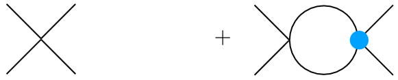
Figure 1: The LO scattering amplitude from the LS equation. The blue circle corresponds to the LO amplitude and the split square is an insertion of the LO separable potential.

4.6 Range corrections with a finite-range scheme: NLO

Recall that treating $a,r\sim\aleph^{-1}$ and $v_{n}\sim{\mathcal{M}}^{-2n+1}$, for $k\ll{\mathcal{M}}$, the ERE of Eq. (1) can be expanded to give the NLO amplitude

$$T_{\scriptscriptstyle{NLO}}(k)\ =\ \frac{4\pi}{M}\left(-\frac{1}{a}+\frac{1}{2}r{k^{2}}-ik\right)^{-2}v_{2}k^{4}\ .$$ (49)

Note that it has been assumed in this expression that $r$ is close to its “physical” value. More generally, and of greater utility when considering realistic NN scattering, one can decompose $r=r_{\scriptscriptstyle{LO}}+r_{\scriptscriptstyle{NLO}}$, where $r_{\scriptscriptstyle{LO}}\sim\aleph^{-1}$ and $r_{\scriptscriptstyle{NLO}}\sim{\mathcal{M}}^{-1}$. In this case

$$T_{\scriptscriptstyle{NLO}}(k)\ =\ \frac{4\pi}{M}\left(-\frac{1}{a}+\frac{1}{2}r_{\scriptscriptstyle{LO}}{k^{2}}-ik\right)^{-2}\textstyle{1\over 2}r_{\scriptscriptstyle{NLO}}k^{2}$$ (50)

so that shape-parameter corrections enter at NNLO (as a subleading contribution to range-squared effects).

The goal in what follows is to generate the NLO amplitudes of Eq. (50) and Eq. (49) (in that order) in the EFT. The LS equation, Eq. (18), for the full scattering amplitude is symbolically expressed as

$$T\ =\ V+V\,G\,T\ ,$$ (51)

where $G$ is the two-particle Green’s function. Expanding the scattering amplitude and potential as

$$T=T_{\scriptscriptstyle{LO}}+T_{\scriptscriptstyle{NLO}}+\ldots\ \ \ ,\ \ \ V=V_{\scriptscriptstyle{LO}}+V_{r}$$ (52)

leads to $T_{\scriptscriptstyle{LO}}$ as an exact solution of the LS equation, as illustrated in Fig. 1, and the NLO and beyond amplitude

$$T_{\scriptscriptstyle{NLO}}\ +\ \ldots=V_{r}+V_{r}\,G\,T_{\scriptscriptstyle{LO}}+T_{\scriptscriptstyle{LO}}\,G\,V_{r}+T_{\scriptscriptstyle{LO}}\,G\,V_{r}\,G\,T_{\scriptscriptstyle{LO}}\ \ldots\ ,$$ (53)

as illustrated diagrammatically to NLO via the Feynman diagrams in Fig. 2. The form of the bare EFT potential $V_{r}$ which matches to the expanded ERE is straightforward to find using the UV/IR symmetry. It is convenient to express the LO potential in the compact form

$$V_{\scriptscriptstyle{LO}}\left(p,p^{\prime}\right)\ =\ C_{\scriptscriptstyle{LO}\,0}\,{\mathcal{G}}(p){\mathcal{G}}(p^{\prime})\ .$$ (54)

where $C_{\scriptscriptstyle{LO}\,0}$ and ${\mathcal{G}}(p^{(\prime)})$ are defined by comparing with Eq. (46). The LO amplitude is then

$$T_{\scriptscriptstyle{LO}}\left(k\right)\ =\ C_{\scriptscriptstyle{LO}\,0}\,{\mathcal{G}}^{2}(k)\,{\bm{Z}}^{-1}\ ,$$ (55)

with ${\bm{Z}}\equiv 1-C_{\scriptscriptstyle{LO}\,0}{\mathbb{I}}_{2}$ and the convergent integral

$${\mathbb{I}}_{2}\ =\ M\int\frac{d^{3}q}{(2\pi)^{3}}\frac{{\mathcal{G}}^{2}(q)}{k^{2}-{q^{2}}+i\epsilon}\ =\ -\frac{M}{4\pi}{\mathcal{G}}^{2}(k)\left(\mu+ik\right).$$ (56)

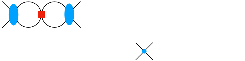
Figure 2: The NLO and beyond scattering amplitude in perturbation theory. The blue circle corresponds to the LO amplitude and the red square is an insertion of the NLO potential.

Now notice that the NLO amplitude of Eq. (50) transforms simply under the momentum inversion $k\mapsto 2/(|ar|k)=\mu\nu/k$ as $T_{\scriptscriptstyle{NLO}}\to T^{*}_{\scriptscriptstyle{NLO}}$ $(ar>0)$ or $T_{\scriptscriptstyle{NLO}}\to T_{\scriptscriptstyle{NLO}}$ $(ar<0)$. Based on the discussion below Eq. (45) it may be expected that the part of $V_{r}$ that generates $T_{\scriptscriptstyle{NLO}}$ will be invariant under momentum inversion up to a sign and $\mu\leftrightarrow\nu$. Consider the energy-dependent potential,

$$k^{2}V_{\scriptscriptstyle{LO}}\left(k,k\right){\mathcal{G}}^{2}(k)\ =\ C_{\scriptscriptstyle{LO}\,0}k^{2}\,{\mathcal{G}}^{4}(k)$$ (57)

which maps to (minus) itself with $\mu\leftrightarrow\nu$ for $ar$ positive (negative) and is therefore a candidate for the piece of $V_{r}$ which generates $T_{\scriptscriptstyle{NLO}}$. An energy-independent residual potential can then be defined as

$$V_{r}(p^{\prime},p)=\big{[}c_{0}+c_{2}\left(p^{2}+p^{\prime 2}\right)+\dots\big{]}V_{\scriptscriptstyle{LO}}\left(p^{\prime},p\right)\left({\mathcal{G}}^{2}(p)+{\mathcal{G}}^{2}(p^{\prime})\right)\ ,$$ (58)

where the $c^{(\prime)}_{m}$ coefficients are bare parameters, subject to renormalization. On-shell this potential has the desired UV/IR transformation properties. Note that the form of the potential reflects that only odd powers of ${\mathcal{G}}(p^{(\prime)})$ in $V_{r}$ will match to a polynomial in $k$ for $k\sim\aleph$. Formally, the (bare) coefficients of the full potential can be expressed for $k\ll\aleph$ as $C^{(\prime)}_{m}=C^{(\prime)}_{\scriptscriptstyle{LO}\,m}+C^{(\prime)}_{\scriptscriptstyle{NLO}\,m}$, where $C^{(\prime)}_{\scriptscriptstyle{NLO}\,m}\equiv C_{\scriptscriptstyle{LO}\,0}\cdot c^{(\prime)}_{m}$.

Evaluating the diagrams of Fig. 2 with a single insertion of $V_{r}$ gives

$$T_{\scriptscriptstyle{NLO}}=2c_{0}C_{\scriptscriptstyle{LO}\,0}{\mathcal{G}}^{2}(k)\,\big{[}{\mathcal{G}}^{2}(k)+C_{\scriptscriptstyle{LO}\,0}{\bm{Z}}^{-1}\left({\mathcal{G}}^{2}(k){\mathbb{I}}_{2}+{\mathbb{I}}_{4}\right)+C^{2}_{\scriptscriptstyle{LO}\,0}{\bm{Z}}^{-2}{\mathbb{I}}_{2}{\mathbb{I}}_{4}\big{]}$$

$$+2c_{2}C_{\scriptscriptstyle{LO}\,0}{\mathcal{G}}^{2}(k)\,\big{\{}2{\mathcal{G}}^{2}(k)k^{2}+C_{\scriptscriptstyle{LO}\,0}{\bm{Z}}^{-1}[{\mathcal{G}}^{2}(k)\left(2k^{2}{\mathbb{I}}_{2}-{\mathbb{J}}_{2}\right)+2k^{2}{\mathbb{I}}_{4}-{\mathbb{J}}_{4}]$$

$$+C^{2}_{\scriptscriptstyle{LO}\,0}{\bm{Z}}^{-2}[2{\mathbb{I}}_{2}{\mathbb{I}}_{4}k^{2}-{\mathbb{I}}_{2}{\mathbb{J}}_{4}-{\mathbb{J}}_{2}{\mathbb{I}}_{4}]\big{\}}$$ (59)

where

$${\mathbb{I}}_{4} = M\int\frac{d^{3}q}{(2\pi)^{3}}\frac{{\mathcal{G}}^{4}(q)}{k^{2}-{q^{2}}+i\epsilon}\ =\ -\frac{M}{4\pi}{\mathcal{G}}^{4}(k)\left(\textstyle{1\over 2}\mu-\frac{k^{2}}{2\mu}+ik\right)\ \ ,$$

$${\mathbb{J}}_{2} = \left(\frac{\omega}{2}\right)^{3-d}M\int\frac{d^{d}q}{(2\pi)^{d}}{\mathcal{G}}^{2}(q)\ \ {\smash{\mathop{{\relbar\joinrel\longrightarrow}}\limits^{\rm PDS}}}\ \ -\frac{M\mu^{2}}{4\pi}\left(\mu-\omega\right)\ \ ,$$

$${\mathbb{J}}_{4} = M\int\frac{d^{3}q}{(2\pi)^{3}}{\mathcal{G}}^{4}(q)\ =\ \frac{M\mu^{3}}{8\pi}\ .$$ (60)

Here the linearly divergent integral ${\mathbb{J}}_{2}$ has been evaluated in dimensional regularization with the PDS scheme Kaplan:1998tg ; Kaplan:1998we , and $\omega$ is the renormalization scale. In terms of renormalized parameters, the amplitude takes the form

$$T_{\scriptscriptstyle{NLO}} = C_{\scriptscriptstyle{LO}\,0}\left({\mathcal{G}}^{2}(k){\bm{Z}}^{-1}\right)^{2}\big{[}c_{0}^{R}\left(1-\zeta\nu/\mu\right)+c_{2}^{R}\left(3-\zeta\nu/\mu\right)k^{2}\big{]}\ ,$$ (61)

where the renormalized parameters, $c^{(\prime)R}_{m}$, are defined as

$$c_{2}^{R} = c_{2}\ \ \ ,\ \ \ c_{0}^{R}\,=\,c_{0}(\omega)+{c_{2}^{R}}\left(\frac{\mu+\zeta\nu}{\mu-\zeta\nu}\right)\big{[}\zeta\mu\nu+\omega\left(\mu-\zeta\nu\right)\big{]}\ .$$ (62)

Matching to the expanded ERE of Eq. (50) gives $c_{0}^{R}=0$ and

$$C_{\scriptscriptstyle{NLO}\,2}\,=\,\frac{M}{4\pi}C^{2}_{\scriptscriptstyle{LO}\,0}\left(3-\zeta\nu/\mu\right)^{-1}\textstyle{1\over 2}r_{\scriptscriptstyle{NLO}}\ ,$$ (63)

with $C^{(\prime)}_{\scriptscriptstyle{NLO}\,m}\,=\,C_{\scriptscriptstyle{LO}\,0}\cdot c^{(\prime)R}_{m}$. This relation gives a subleading enhancement of the same form as the usual pionless EFT vanKolck:1998bw ; Kaplan:1998tg ; Kaplan:1998we up to the factor in parenthesis, and results in the scaling

$$c_{2}^{R}\ \sim\ \frac{1}{{\mathcal{M}}\aleph}\ \ \ ,\ \ \ C_{\scriptscriptstyle{NLO}\,2}\sim\frac{4\pi}{M{\mathcal{M}}\aleph^{2}}\ .$$ (64)

In similar fashion, the NLO amplitude of Eq. (49) can be obtained via the energy-independent residual potential

$$V_{r}(p^{\prime},p) = \big{[}c_{0}+c_{2}\left(p^{2}+p^{\prime 2}\right)+c_{4}\left(p^{4}+p^{\prime 4}\right)+c^{\prime}_{4}p^{2}p^{\prime 2}+\dots\big{]}$$ (65)

$$\times V_{\scriptscriptstyle{LO}}\left(p^{\prime},p\right)\left({\mathcal{G}}^{2}(p)+{\mathcal{G}}^{2}(p^{\prime})\right)\ .$$

Working in dimensional regularization with $\overline{\textstyle{MS}}$, the amplitude takes the form

$$T_{\scriptscriptstyle{NLO}} = C_{\scriptscriptstyle{LO}\,0}\left({\mathcal{G}}^{2}(k){\bm{Z}}^{-1}\right)^{2}\big{[}c_{0}^{R}\left(1-\zeta\nu/\mu\right)+c_{2}^{R}\left(3-\zeta\nu/\mu\right)k^{2}$$ (66)

$$\qquad\qquad\qquad\qquad\qquad\qquad\qquad+[2c_{4}^{\prime R}+c_{4}^{R}\left(3-\zeta\nu/\mu\right)]k^{4}\big{]}\ ,$$

with the renormalized parameters

$$c^{(\prime)R}_{4} = c^{(\prime)}_{4}\ \ \ ,\ \ \ c_{2}^{R}\,=\,c_{2}-\mu\left(\mu+\zeta\nu\right)\big{[}c_{4}^{R}+\left(3-\zeta\nu/\mu\right)^{-1}c_{4}^{\prime R}\big{]}\ ,$$

$$c_{0}^{R} = c_{0}-\mu\left(\frac{\mu+\zeta\nu}{\mu-\zeta\nu}\right)\big{[}-c_{2}\nu\zeta+c_{4}^{R}\mu^{2}(2\mu+\nu\zeta)+c_{4}^{\prime R}\mu^{2}(\mu+\nu\zeta)\big{]}\,.$$ (67)

Matching to the expanded ERE of Eq. (49) now gives $c_{0}^{R}=c_{2}^{R}=0$ and

$$C_{\scriptscriptstyle{NLO}\,4}+2C_{\scriptscriptstyle{NLO}\,4}^{\prime}\left(3-\zeta\nu/\mu\right)^{-1} = \frac{M}{4\pi}C^{2}_{\scriptscriptstyle{LO}\,0}\left(3-\zeta\nu/\mu\right)^{-1}v_{2}.$$ (68)

The coefficients scale as

$$c_{4}^{(\prime)R}\ \sim\ \frac{1}{{\mathcal{M}}^{3}\aleph}\ \ \ ,\ \ \ C^{(\prime)}_{\scriptscriptstyle{NLO}\,4}\sim\frac{4\pi}{M{\mathcal{M}}^{3}\aleph^{2}}\ .$$ (69)

This differs from the conventional pionless theory counting which has a nominally leading contribution to the $C^{(\prime)}_{4}$ operators from effective range (squared) effects.

5 EFT description: the NN s-wave phase shifts

The phase shifts to NLO in the EFT expansion are

$$\delta_{s}(k) = \delta_{\scriptscriptstyle{LO}\,(s)}(k)\,+\,\delta_{\scriptscriptstyle{NLO}\,(s)}(k)\ ,$$ (70)

with

$$\delta_{\scriptscriptstyle{LO}\,(s)}(k) = -\frac{1}{2}i\ln\left(1\ -\ i\frac{kM}{2\pi}T_{\scriptscriptstyle{LO}\,(s)}(k)\right)\ ,$$ (71)

$$\delta_{\scriptscriptstyle{NLO}\,(s)}(k) = -\frac{kM}{4\pi}T_{\scriptscriptstyle{NLO}\,(s)}(k)\left(1\ -\ i\frac{kM}{2\pi}T_{\scriptscriptstyle{LO}\,(s)}(k)\right)^{-1}\ .$$ (72)

Recall from section 3 that in s-wave NN scattering, the UV/IR symmetry of the full $S$-matrix requires range corrections that are correlated with the scattering lengths and treated exactly. The physical effective ranges can therefore be expressed as $r_{s}=r_{\scriptscriptstyle{LO}\,(s)}+r_{\scriptscriptstyle{NLO}\,(s)}$ with

$$r_{\scriptscriptstyle{LO}\,(0)} = 2\lambda a_{1}\ \ \ ,\ \ \ r_{\scriptscriptstyle{LO}\,(1)}\,=\,-2\lambda a_{0}\ .$$ (73)

The singlet and triplet phase shifts with the NLO amplitude given by Eq. (50) are plotted in Fig. (3). At LO, there are three parameters given by the two s-wave scattering lengths and $\lambda$, which is fixed to $\lambda=0.14\pm 0.11$, the range of values that exactly encompasses fits of $\lambda$ to each s-wave channel independently. This spread in $\lambda$ corresponds to the shaded gray region of the figures and is a conservative estimate of the LO uncertainty. The NLO curve has been generated by tuning the $r_{\scriptscriptstyle{NLO}\,(s)}$ to give the “physical” effective ranges. A band on the NLO curves can easily be set by folding in the nominally NNLO effect.

The singlet and triplet phase shifts with the NLO amplitude given by Eq. (49) are plotted in Fig. (4). As this treats both effective ranges exactly it provides an extremely accurate fit to the phase shifts due to the smallness of the shape parameters.

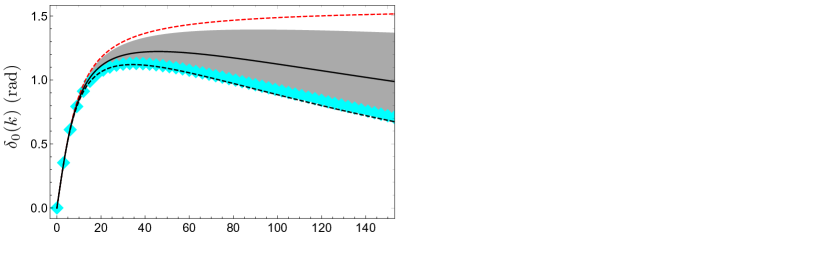
Figure 3: Singlet (left panel) and triplet (right panel) s-wave NN phase shifts with the NLO amplitudes given by Eq. (50) plotted versus center-of-mass momentum $k$. The cyan polygons are the Nijmegen phase shift analysis (PWA93) NNOnline . The red dashed curve is the LO phase shift in the pionless theory (scattering length only). The solid black curve is the central value of the LO phase shifts with exact UV/IR symmetry. The gray region represents an error band for the black curve and the dashed black curve is the NLO curve.

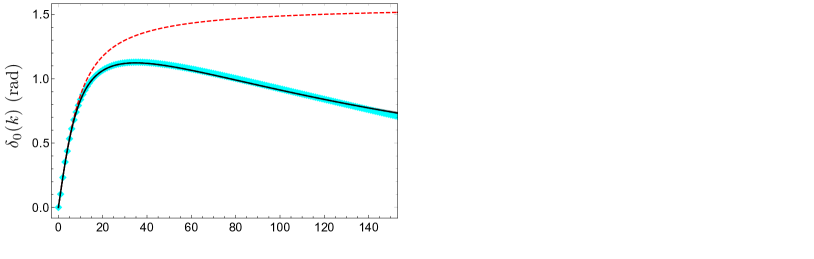
Figure 4: Same as in Fig. (3) but with the effective ranges treated exactly in each channel and the NLO amplitudes given by Eq. (49). In both channels, the NLO curve overlaps with the central value of the LO phase shift.

6 Conclusion

The s-wave NN $S$-matrix obtained from the ERE with scattering length and effective range terms only, has interesting UV/IR symmetries which are special inversions of the momenta. These symmetries set the region of applicability of the EFT descriptions. For instance, while it is common to view the EFT of large scattering lengths as an expansion about the unitary fixed point of the RG, it is, strictly speaking, an expansion about the fixed point of a momentum inversion symmetry. The UV/IR symmetries, while not symmetries of the EFT action or of the scattering amplitude, are present in the interaction. For instance, in the EFT of large scattering lengths, the UV/IR symmetry is manifest in the RG flow of the contact operator as an inversion symmetry of the RG scale which interchanges the trivial and unitary RG fixed points and leaves the beta function invariant Beane:2021xrk . When the effective range is also treated at LO in the EFT, the $S$-matrix has a (distinct) UV/IR symmetry which effectively determines the LO potential, and constrains the form of the perturbative NLO corrections.

There are many avenues to pursue with this new EFT. For instance, the softened asymptotic behavior of the LO potential may resolve the issues of renormalization that arise when range corrections are added to the integral equations that describe the three-nucleon system at very low energies. In addition, given the improved convergence of LO in the EFT up to momenta beyond the range of validity of the pionless EFT, the perturbative pion paradigm may be worth revisiting in this scheme. It may also be the case that the UV/IR symmetries have interesting consequences for systems of many nucleons near unitarity.

- (1) S. Weinberg, Physica A 96(1-2), 327 (1979). DOI 10.1016/0378-4371(79)90223-1
- (2) J. Gasser, H. Leutwyler, Annals Phys. 158, 142 (1984). DOI 10.1016/0003-4916(84)90242-2
- (3) S. Weinberg, Phys. Lett. B251, 288 (1990). DOI 10.1016/0370-2693(90)90938-3
- (4) S. Weinberg, Nucl. Phys. B 363, 3 (1991). DOI 10.1016/0550-3213(91)90231-L
- (5) S. Weinberg, Phys. Lett. B 295, 114 (1992). DOI 10.1016/0370-2693(92)90099-P
- (6) C. Ordonez, U. van Kolck, Phys. Lett. B 291, 459 (1992). DOI 10.1016/0370-2693(92)91404-W
- (7) C. Ordoñez, L. Ray, U. van Kolck, Phys. Rev. Lett. 72, 1982 (1994). DOI 10.1103/PhysRevLett.72.1982
- (8) C. Ordoñez, L. Ray, U. van Kolck, Phys. Rev. C 53, 2086 (1996). DOI 10.1103/PhysRevC.53.2086
- (9) D.B. Kaplan, M.J. Savage, M.B. Wise, Nucl. Phys. B 478, 629 (1996). DOI 10.1016/0550-3213(96)00357-4
- (10) A. Nogga, R.G.E. Timmermans, U. van Kolck, Phys. Rev. C 72, 054006 (2005). DOI 10.1103/PhysRevC.72.054006
- (11) S. Beane, P.F. Bedaque, M. Savage, U. van Kolck, Nucl. Phys. A 700, 377 (2002). DOI 10.1016/S0375-9474(01)01324-0
- (12) M. Pavón Valderrama, M. Sánchez Sánchez, C.J. Yang, B. Long, J. Carbonell, U. van Kolck, Phys. Rev. C 95(5), 054001 (2017). DOI 10.1103/PhysRevC.95.054001
- (13) U. van Kolck, Front. in Phys. 8, 79 (2020). DOI 10.3389/fphy.2020.00079
- (14) E. Epelbaum, H.W. Hammer, U.G. Meißner, Rev. Mod. Phys. 81, 1773 (2009). DOI 10.1103/RevModPhys.81.1773
- (15) R. Machleidt, D.R. Entem, Phys. Rept. 503, 1 (2011). DOI 10.1016/j.physrep.2011.02.001
- (16) E. Epelbaum, J. Gegelia, U.G. Meißner, Nucl. Phys. B 925, 161 (2017). DOI 10.1016/j.nuclphysb.2017.10.008
- (17) E. Epelbaum, J. Gegelia, U.G. Meißner, Commun. Theor. Phys. 69(3), 303 (2018). DOI 10.1088/0253-6102/69/3/303
- (18) E. Epelbaum, A.M. Gasparyan, J. Gegelia, U.G. Meißner, Eur. Phys. J. A 54(11), 186 (2018). DOI 10.1140/epja/i2018-12632-1
- (19) E. Epelbaum, A.M. Gasparyan, J. Gegelia, U.G. Meißner, Eur. Phys. J. A 55, 56 (2019). DOI 10.1140/epja/i2019-12751-1
- (20) E. Epelbaum, A.M. Gasparyan, J. Gegelia, U.G. Meißner, X.L. Ren, Eur. Phys. J. A 56(5), 152 (2020). DOI 10.1140/epja/s10050-020-00162-4
- (21) M. Pavon Valderrama, Eur. Phys. J. A 55(4), 55 (2019). DOI 10.1140/epja/i2019-12703-9
- (22) D.B. Kaplan, M.J. Savage, M.B. Wise, Phys. Lett. B424, 390 (1998). DOI 10.1016/S0370-2693(98)00210-X
- (23) D.B. Kaplan, M.J. Savage, M.B. Wise, Nucl. Phys. B534, 329 (1998). DOI 10.1016/S0550-3213(98)00440-4
- (24) S. Fleming, T. Mehen, I.W. Stewart, Nucl. Phys. A 677, 313 (2000). DOI 10.1016/S0375-9474(00)00221-9
- (25) U. van Kolck, Nucl. Phys. A645, 273 (1999). DOI 10.1016/S0375-9474(98)00612-5
- (26) M.C. Birse, J.A. McGovern, K.G. Richardson, Phys. Lett. B 464, 169 (1999). DOI 10.1016/S0370-2693(99)00991-0
- (27) C.A. Bertulani, H.W. Hammer, U. Van Kolck, Nucl. Phys. A 712, 37 (2002). DOI 10.1016/S0375-9474(02)01270-8
- (28) H.W. Hammer, C. Ji, D.R. Phillips, J. Phys. G 44(10), 103002 (2017). DOI 10.1088/1361-6471/aa83db
- (29) S.R. Beane, T.D. Cohen, D.R. Phillips, Nucl. Phys. A 632, 445 (1998). DOI 10.1016/S0375-9474(98)00007-4
- (30) D.R. Phillips, T.D. Cohen, Phys. Lett. B 390, 7 (1997). DOI 10.1016/S0370-2693(96)01411-6
- (31) K.A. Scaldeferri, D.R. Phillips, C.W. Kao, T.D. Cohen, Phys. Rev. C 56, 679 (1997). DOI 10.1103/PhysRevC.56.679
- (32) D.R. Phillips, S.R. Beane, T.D. Cohen, Annals Phys. 263, 255 (1998). DOI 10.1006/aphy.1997.5771
- (33) H.W. Hammer, D. Lee, Annals Phys. 325, 2212 (2010). DOI 10.1016/j.aop.2010.06.006
- (34) E.P. Wigner, Phys. Rev. 98, 145 (1955). DOI 10.1103/PhysRev.98.145
- (35) J.B. Habashi, S. Sen, S. Fleming, U. van Kolck, Annals Phys. 422, 168283 (2020). DOI 10.1016/j.aop.2020.168283
- (36) J.W. Chen, G. Rupak, M.J. Savage, Nucl. Phys. A 653, 386 (1999). DOI 10.1016/S0375-9474(99)00298-5
- (37) H.W. Hammer, S. König, U. van Kolck, Rev. Mod. Phys. 92(2), 025004 (2020). DOI 10.1103/RevModPhys.92.025004
- (38) J. Gegelia, Phys. Lett. B 429, 227 (1998). DOI 10.1016/S0370-2693(98)00460-2
- (39) D.R. Phillips, G. Rupak, M.J. Savage, Phys. Lett. B 473, 209 (2000). DOI 10.1016/S0370-2693(99)01496-3
- (40) J. Gegelia, G. Japaridze, Phys. Lett. B 517, 476 (2001). DOI 10.1016/S0370-2693(01)00981-9
- (41) M. Sánchez Sánchez, C.J. Yang, B. Long, U. van Kolck, Phys. Rev. C 97(2), 024001 (2018). DOI 10.1103/PhysRevC.97.024001
- (42) D.B. Kaplan, J.V. Steele, Phys. Rev. C 60, 064002 (1999). DOI 10.1103/PhysRevC.60.064002
- (43) D.B. Kaplan, Nucl. Phys. B 494, 471 (1997). DOI 10.1016/S0550-3213(97)00178-8
- (44) S.R. Beane, M.J. Savage, Nucl. Phys. A 694, 511 (2001). DOI 10.1016/S0375-9474(01)01088-0
- (45) T. Mehen, I.W. Stewart, M.B. Wise, Phys. Lett. B 474, 145 (2000). DOI 10.1016/S0370-2693(00)00006-X
- (46) S.R. Beane, R.C. Farrell, Annals of Physics 433, 168581 (2021). DOI https://doi.org/10.1016/j.aop.2021.168581
- (47) S.R. Beane, R.C. Farrell. Causality and dimensionality in geometric scattering (2021)
- (48) S.R. Beane, R.C. Farrell. UV/IR symmetries of the -matrix and RG flow (2021)
- (49) S.R. Beane, D.B. Kaplan, N. Klco, M.J. Savage, Phys. Rev. Lett. 122(10), 102001 (2019). DOI 10.1103/PhysRevLett.122.102001
- (50) J.J. de Swart, C.P.F. Terheggen, V.G.J. Stoks, in 3rd International Symposium on Dubna Deuteron 95 (1995)
- (51) Y. Yamaguchi, Phys. Rev. 95, 1628 (1954). DOI 10.1103/PhysRev.95.1628
- (52) D.R. Phillips, I.R. Afnan, A.G. Henry-Edwards, Phys. Rev. C 61, 044002 (2000). DOI 10.1103/PhysRevC.61.044002
- (53) R.U. Nijmegen. NN-online. http://nn-online.org/ (2005). Accessed: 2018-12-01