Thermodynamic constraints on the nonequilibrium response of one-dimensional diffusions

Abstract

We analyze the static response to perturbations of nonequilibrium steady states that can be modeled as one-dimensional diffusions on the circle. We demonstrate that an arbitrary perturbation can be broken up into a combination of three specific classes of perturbations that can be fruitfully addressed individually. For each class, we derive a simple formula that quantitatively characterizes the response in terms of the strength of nonequilibrium driving valid arbitrarily far from equilibrium.

Introduction. Linear response theory developed as a tool to rationalize the response of equilibrium systems to external perturbations and internal fluctuations. Its central organizing prediction, the fluctuation-dissipation theorem (FDT) Kubo et al. (1985), characterizes such response in terms of experimentally measurable equilibrium correlation functions. This result has been immensely useful, helping to form the statistical-mechanical foundation of hydrodynamics, establishing Green-Kubo relations Kadanoff and Martin (1963); Forster (1975), as well as providing the theoretical scaffolding for light scattering and microrheology experiments Chaikin and Lubensky (1995).

Motivated by these early successes, it is now customary to probe a system’s behavior, no matter how far from equilibrium, in terms of responses to perturbations and correlation functions. Examples can be found in studies of active matter Fily and Marchetti (2012); Bialké et al. (2013); Martin et al. (2001); Mizuno et al. (2007) as well as in analyses of biological function Sato et al. (2003); Murugan et al. (2011); Qian (2012); Yan and Hsu (2013); Hartich et al. (2015); Estrada et al. (2016). However, without the simplicity of the equilibrium FDT as a guiding principle, disparate analysis methods have emerged. One approach has been to re-establish the connection between response and correlation functions around nonequilibrium steady states Agarwal (1972). While the correlation functions require detailed knowledge of the system’s microscopic dynamics, recent theoretical insights from stochastic thermodynamics have provided them with crisp physical interpretations in terms of stochastic entropy production and dynamical activity Prost et al. (2009); Baiesi et al. (2009); Seifert and Speck (2010). A complementary approach has been to characterize violations of the equilibrium-version of the FDT, either through the introduction of effective temperatures Ben-Isaac et al. (2011); Cugliandolo (2011); Dieterich et al. (2015) or for Brownian particles by connecting the violation directly to the steady state entropy production via the Harada-Sasa equality Harada and Sasa (2005); Toyabe et al. (2010).

In the tradition of studying violations of the FDT, one of us recently demonstrated that the magnitude of the response to an external perturbation can be quantitatively constrained by the degree of nonequilibrium driving Owen et al. (2020). These predictions were limited to static (or zero-frequency) response in nonequilibrium steady states that could be modeled as discrete continuous-time Markov jump processes with a finite number of states. In this article, we expand this framework to the static response of nonequilibrium steady states described by one-dimensional diffusion processes with periodic boundary conditions. This class of systems not only encompasses a variety of experimental situations, such as a driven colloidal particle in a viscous fluid Speck et al. (2007); Joubaud et al. (2008); Gomez-Solano et al. (2009), but is also analytically tractable, which has made it a paradigmatic theoretical model within stochastic thermodynamics Seifert (2012).

Our main contribution is to unravel an arbitrary perturbation of a diffusive steady state into a linear combination of three classes of perturbations that can be individually analyzed. For each class we prove an equality or inequality that quantifies how thermodynamics and nonequilibrium driving constrain the response.

Setup. Our focus is a single periodic degree of freedom $x$ that evolves diffusively on a circle of length $L$. The dynamics are completely characterized by the probability density $\rho(x,t)$ as a function of time $t$ and position $x$ whose evolution is governed by the generic Fokker-Planck equation Gardiner (2004),

$$\begin{split}\partial_{t}\rho(x,t)&=-\partial_{x}[A(x)\rho(x,t)]+\partial_{x}[B(x)\partial_{x}\rho(x,t)]\\ &\equiv\hat{\mathcal{L}}\rho(x,t),\end{split}$$ (1)

with periodic functions $A(x)$ and $B(x)$. Equation (1) has a unique steady state distribution $\pi(x)$, given as the periodic solution of $\hat{\mathcal{L}}\pi(x)=0$. In general, $\pi(x)$ represents a nonequilibrium steady state. However, when the functions $A(x)$ and $B(x)$ satisfy the potential condition $\int_{0}^{L}A(z)/B(z)dz=0$, the dynamics are detailed balanced and the resulting steady state describes an equilibrium situation $\pi^{\rm eq}(x)\propto e^{\psi(x)}$ with conservative potential $\psi(x)=\int_{0}^{x}A(z)/B(z)dz$ Gardiner (2004). Indeed, the magnitude of the breaking of the potential condition can be identified with the thermodynamic force ${\mathcal{F}}=\int_{0}^{L}A(z)/B(z)dz$ driving the system away from equilibrium, when the dynamics are thermodynamically consistent Polettini et al. (2016a, b).

Parametrizing steady-state response. Our aim is to characterize how steady state averages of observables $\langle Q\rangle=\int_{0}^{L}Q(z)\pi(z)dz$ change in response to variations in $A(x)$ and $B(x)$. Our main contribution here is to recognize that it is useful to parametrize changes in the dynamics with a constant $f$ and two periodic functions $\mu(x)$ and $U(x)$ via $A(x)=\mu(x)[-U^{\prime}(x)+f]$ and $B(x)=\mu(x)$:

$$\hat{\mathcal{L}}\rho=-\partial_{x}{\mu(x)[-U^{\prime}(x)+f]\rho}+\partial_{x}[\mu(x)\partial_{x}\rho].$$ (2)

We were led to this parametrization by first discretizing the diffusion process and then comparing the result to the decomposition introduced previously in Owen et al. (2020) for discrete Markov jump processes. This mapping then suggested that derivatives with respect to $\mu$, $U$, and $f$ could have interesting thermodynamic limits. While the analysis here is completely self-contained given the definitions in (2), we do include for reference the discretization mapping in SM .

More general perturbations in $A(x)$ and $B(x)$ can then be built up as linear combinations of changes in $\mu$, $U$ and $f$. Indeed, if we perturb the dynamics by making infinitesimal changes $A(x)\to A(x)+\delta A(x)$ and $B(x)\to B(x)+\delta B(x)$, then changes in our parameters can be conveniently expressed in terms of $\Delta(x)=[\delta A(x)B(x)-\delta B(x)A(x)]/B(x)^{2}$ as SM

$$\delta\mu(x)=\delta B(x),$$ (3)

$$\delta U(x)=-\int_{0}^{x}\Delta(z)\ dz+\frac{x}{L}\int_{0}^{L}\Delta(z)\ dz+\delta U(0),$$ (4)

$$\delta f=\frac{1}{L}\int_{0}^{L}\Delta(z)\ dz,$$ (5)

where $\delta U(0)$ is an undetermined constant, which does not affect the predictions.

While our parametrization is a mathematical convenience, the notation here is meant to bring to mind the equation of motion of a colloidal particle in a viscous fluid at (dimensionless) temperature $k_{B}T=1$ with spatially-dependent mobility $\mu(x)$ moving in an energy landscape $U(x)$ driven by a constant nonconservative mechanical force $f$. We will rely on this analogy for intuition, and often use this terminology. However, we stress that this is only a mathematical equivalence and our analysis is not restricted to a single overdamped particle, but applies to any physical system that can be accurately modeled as a one-dimensional diffusion. Indeed, any model specified by $A(x)$ and $B(x)$ can be mapped to our parametrization. Moreover, our decomposition captures the most general separation of the dynamics into a conservative contribution $U(x)$ and a nonconservative contribution $f$. This highlights the fact that the only way to break the potential condition is the inclusion of a force with a constant contribution $f$, with the resulting thermodynamic force ${\mathcal{F}}=\int_{0}^{L}A(z)/B(z)dz=fL$. Thermodynamic equilibrium is then characterized by $f=\frac{1}{L}\int_{0}^{L}A(z)/B(z)dz=0$, in which case the steady-state distribution takes the Gibbs form $\pi^{\rm eq}(x)\propto e^{-U(x)}$ in terms of the (dimensionless) energy landscape. From this point of view, perturbations of $A$ and $B$ usually amount to affecting only $U$ or $f$ Baiesi and Maes (2013). We find here that by allowing for perturbations in $\mu$ in our theoretical analysis, we are able to unravel simple limits on response, even if perturbations that end up only affecting $\mu$ in experimental settings may not be common. Our main predictions are then a series of equalities and inequalities for the steady state averages of observables due to perturbations in our three functions $\mu$, $U$, and $f$.

Our first prediction is an equality for the response of an arbitrary observable $Q$ to a coupled $U$ and $\mu$ perturbation,

$$\frac{\delta\langle Q\rangle}{\delta U(y)}+\frac{\delta\langle Q\rangle}{\delta\ln\mu(y)}=-\pi(y)[Q(y)-\langle Q\rangle].$$ (6)

For $\mu$-perturbations, we derive an inequality on the ratio of the averages of two nonnegative observables $Q_{1}$ and $Q_{2}$ ($Q_{1},Q_{2}\geq 0$),

$$\left|\int_{a}^{b}\frac{\delta\ln(\langle Q_{1}\rangle/\langle Q_{2}\rangle)}{\delta\ln\mu(z)}\ dz\right|\leq\tanh(|{\mathcal{F}}|/4).$$ (7)

Note that the restriction to non-negative observables does not pose any serious limitation as we can always shift any observable by its minimum to create a non-negative one.

Last, we find that constraints on $f$ perturbations can most naturally be expressed as responses to the thermodynamic force ${\mathcal{F}}=fL$,

$$\left|\frac{\partial\ln(\langle Q_{1}\rangle/\langle Q_{2}\rangle)}{\partial{\mathcal{F}}}\right|\leq 1.$$ (8)

By exploiting the freedom to choose the observables $Q_{1}$ and $Q_{2}$, we can arrive at bounds for a variety of quantities of interest. For example, the choice $Q_{1}(z;x)=\delta(z-x)$ and $Q_{2}=1$, gives bounds on the response of the steady-state density

$$\left|\int_{a}^{b}\frac{\delta\ln\pi(x)}{\delta\ln\mu(z)}\ dz\right|\leq\tanh(|{\mathcal{F}}|/4),\$$ (9)

$$\left|\frac{\partial\ln\pi(x)}{\partial{\mathcal{F}}}\right|\leq 1.$$ (10)

We obtain our results by differentiating the known analytic expression for the steady state distribution Gardiner (2004),

$$\begin{split}\pi(x)&=\frac{e^{-U(x)+fx}}{\mathcal{N}}\Bigg{[}e^{-fL}\int_{0}^{x}e^{U(z)-fz-\ln\mu(z)}dz\\ &~{}~{}~{}~{}~{}~{}~{}~{}~{}~{}~{}~{}~{}~{}~{}~{}~{}~{}~{}~{}~{}+\int_{x}^{L}e^{U(z)-fz-\ln\mu(z)}dz\Bigg{]},\end{split}$$ (11)

with ${\mathcal{N}}$ a normalization constant, and then reasoning about the result. Derivations are presented in SM . Here, we examine and illustrate these formulas.

Equilibrium-like FDT. At thermodynamic equilibrium (${\mathcal{F}}=0$), the response to perturbations in the energy landscape $U(x)$ is well characterized by the FDT in terms of equilibrium correlation functions. Imagine we perturb an equilibrium system by slightly altering an externally controllable parameter $\lambda$ that affects the energy as $U_{\lambda}(x)=U(x)-\lambda V(x)$, which defines the coordinate conjugate to the perturbation $V(x)$. The equilibrium FDT then predicts that the response of an arbitrary observable $Q(x)$ can be expressed as Marconi et al. (2008)

$$\partial_{\lambda}\langle Q\rangle={\rm Cov}_{\rm eq}(Q,V),$$ (12)

in terms of the fluctuations via the equilibrium covariance ${\rm Cov}_{\rm eq}(Q,V)=\langle QV\rangle_{\rm eq}-\langle Q\rangle_{\rm eq}\langle V\rangle_{\rm eq}$.

Away from thermodynamic equilibrium (${\mathcal{F}}\neq 0$), the response to $U(x)$ perturbations is generally more challenging to characterize. However, when we combine changes in $U$ with $\mu$ as in (6), we find a response that is exactly equivalent to the response of an equilibrium Gibbs distribution to changes in $U$ alone. We can exploit this observation by considering a perturbation that is equivalent to varying the energy and mobility in concert as $U_{\lambda}(x)=U(x)-\lambda V(x)$ and $\mu_{\lambda}(x)=\mu(x)[1-\lambda V(x)]$. In this case, the response is

$$\partial_{\lambda}\langle Q\rangle =-\int_{0}^{L}V(z)\left[\frac{\delta\langle Q\rangle}{\delta U(z)}+\frac{\delta\langle Q\rangle}{\delta\ln\mu(z)}\right]\ dz.$$ (13)

A direct application of (6) then allows us to interpret the result as a simple FDT-like expression

$$\partial_{\lambda}\langle Q\rangle={\rm Cov}(Q,V),$$ (14)

where significantly the response is given by the nonequilibrium covariance between the observable and the conjugate coordinate, ${\rm Cov}(Q,V)=\langle QV\rangle-\langle Q\rangle\langle V\rangle$. This result demonstrates that for a class of perturbations—where $U$ and $\mu$ are varied in unison—the FDT holds in its equilibrium form, arbitrarily far from equilibrium. That an equilibrium-like FDT held for certain time-dependent perturbations of diffusion processes was previously observed by Graham Graham (1977). Recently, we have extended this observation to arbitrary Markov processes Chun et al. (2021). The value in rederiving this static response formula here is that it highlights its role as an important component of a more general framework for analyzing nonequilibrium response.

Energy perturbations. Changes in the energy function $U$ represent a customary perturbation applied to probe a system’s steady state. While it can be challenging to interpret expressions for the response in this case, we can combine the predictions in (6) and (7) to find simple thermodynamic constraints.

To apply our results, we have to focus on a perturbation where we shift the energy uniformly on a fixed interval $x\in[a,b]$ (Fig. 1): specifically, $U_{\lambda}(x)=U(x)-\lambda I_{[a,b]}(x)$, where $I_{A}(z)$ is the indicator function taking the value $1$ when $z$ is in the set $A$ and $0$ otherwise.

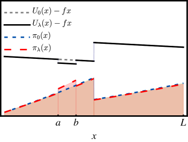
Figure 1: Example of perturbing the energy landscape: Pictured is the “effective potential” as a function of position $x$ before the perturbation $U_{0}(x)-fx$ (gray dashed) and after lowering the energy in the region $x\in[a,b]$ by $\lambda I_{[a,b]}(x)$ (black). This shifts the steady state distribution $\pi(x)$ from the orange dotted curve to the red long-dashed curve.

Our question is then how thermodynamics constrains the nonequilibrium response $R^{\rm neq}_{Q,U}=\partial_{\lambda}\langle Q\rangle=-\int_{a}^{b}\delta\langle Q\rangle/\delta U(z)dz$ of a (nonnegative) observable $Q$ to perturbations in $U$ with fixed thermodynamic driving ${\mathcal{F}}$. Before addressing this question, however, let us first remind ourselves what a naive application of the FDT would have predicted, namely that the response would be given by the covariance between the observable $Q(x)$ and the conjugate coordinate $I_{[a,b]}(x)$ as $R_{Q,U}^{\rm eq}={\rm Cov}\left(Q,I_{[a,b]}\right)$.

Now, let us proceed with perturbations of a nonequilibrium steady state (${\mathcal{F}}\neq 0$). Observe that $U$ perturbations can be built from the sum

$$\begin{split}R^{\rm neq}_{Q,U}&=-\int_{a}^{b}\frac{\delta\langle Q\rangle}{\delta U(z)}dz\\ &=-\int_{a}^{b}\left[\frac{\delta\langle Q\rangle}{\delta U(z)}+\frac{\delta\langle Q\rangle}{\delta\ln\mu(z)}\right]-\frac{\delta\langle Q\rangle}{\delta\ln\mu(z)}dz.\end{split}$$ (15)

The first term is our coupled $\mu$-$U$ perturbation (13) that satisfies an equilibrium-like FDT (14) and is therefore equal to the covariance between the observable $Q$ and the conjugate coordinate $I_{[a,b]}$, ${\rm Cov}\left(Q,I_{[a,b]}\right)$, which is exactly the same as our naive prediction for the equilibrium response $R_{Q,U}^{\rm eq}$. The remaining contribution can be constrained by the thermodynamic force using (7) with the choices $Q_{1}(x)=Q(x)$ and $Q_{2}(x)=1$,

$$\big{|}R^{\rm neq}_{Q,U}-R^{\rm eq}_{Q,U}\big{|} =\left|\langle Q\rangle\int_{a}^{b}\frac{\delta\ln\langle Q\rangle}{\delta\ln\mu(z)}dz\right|$$

$$\leq\langle Q\rangle\tanh(|\mathcal{F}|/4).$$ (16)

The farther the system is from equilibrium, as measured by the force ${\mathcal{F}}$, the larger the possible nonequilibrium response. Alternatively, since $R^{\rm eq}_{Q,U}$ is the naive prediction from the FDT, we can interpret (16) as a quantitative bound on the violation of the FDT in terms of the nonequilibrium driving.

To illustrate this prediction, we analyzed the response of the steady-state density $\pi(x)$ itself, corresponding to the observable $Q(z;x)=\delta(z-x)$. Denoting this response with a slight abuse of notation as $R^{\rm neq}_{x,U}$, the operative form of (16) is

$$\big{|}R^{\rm neq}_{x,U}-R^{\rm eq}_{x,U}\big{|}\leq\pi(x)\tanh(|{\mathcal{F}}|/4)$$ (17)

We choose perturbations of the energy landscape of the form $U(x)=U_{0}\Theta(x-L/2)$ where $\Theta(x-L/2)$ is the Heaviside step function and $U_{0}\in\{1,2,3\}$ is a constant (Fig. 1). We further fix the mobility $\mu(x)=1$ and set the circumference of the circle to $L=1$. We numerically evaluated the response $R^{\rm neq}_{x,U}$ to energy perturbations on the interval $[x,b]$ as a function of ${\mathcal{F}}=f$ for 100 combinations of $x$ and $b$ each sampled uniformly on the unit interval $[0,1]$. We have chosen the observation position $x$ to be on the edge of the perturbation region in order to enhance the sampling of highly responsive scenarios.

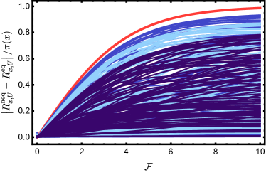
Figure 2: Illustration of energy-perturbation thermodynamic bound: Normalized deviation of nonequilibrium response $\big{|}R^{\rm neq}_{x,U}-R^{\rm eq}_{x,U}\big{|}/\pi(x)$ at position $x$ for energy perturbations on the interval $[a,b]$ from an energy landscape $U(x)=U_{0}\Theta(x-L/2)$ given by the Heaviside step function multiplied by $U_{0}=1$ (dark blue), $2$ (light blue), $3$ (blue). Each color contains 100 randomly sampled pairs $(x=a)$ on the unit square. All curves fall below the predicted bound $\tanh(|{\mathcal{F}}|/4)$ (red line). Other parameters: $L=1$ and $\mu(x)=1$.

The results presented in Fig. 2 verify that for all sampled parameter combinations the normalized deviation $\big{|}R^{\rm neq}_{x,U}-R^{\rm eq}_{x,U}\big{|}/\pi(x)$ remains below the predicted bound $\tanh(|{\mathcal{F}}|/4)$.

Discussion. We have observed that any perturbation of a one-dimensional diffusion can be broken up into a linear combination of three types, which we term energy-mobility perturbations, mobility perturbations, and force perturbations. For each class, we have derived either an equality or inequality characterizing the response in terms of the strength of the nonequilibrium driving. One could have arrived at these predictions by discretizing the diffusion process and then using the bounds for discrete Markov dynamics reported previously in Owen et al. (2020). For completeness, we carry out this program explicitly in SM , but note here that it requires a careful analysis of the limiting procedure. In light of this, our self-contained analysis based on the Fokker-Planck equation offers a more direct approach.

At the moment the analysis is limited in a handful of important ways. Our current methodology only works for one-dimensional systems, since it is based on examining the analytic solution for the steady-state distribution, which is not known for higher-dimensional systems. Moreover, discretizing higher-dimensional diffusions and then using the bounds reported in Owen et al. (2020) will not help either. We have checked that those inequalities are not sufficiently strong to provide useful limitations SM . Even still, our results are suggestive that there is some thermodynamic structure in the nonequilibrium response of higher-dimensional diffusions, but it still remains to be investigated.

We have also limited our discussion to the response of state observables $Q(x)$ that are functions only of the system’s position. The response of current observables, such as the velocity of the system, is an important extension of the current approach. Earlier studies on the Einstein relation connecting the velocity response (mobility) and diffusion coefficient for diffusive nonequilibrium steady states have also revealed FDT-like inequalities Baiesi et al. (2011); Dechant (2018); Dechant and Sasa (2020). Together these predictions suggest that there are also quantitative bounds on the response of generic current observables in terms of the thermodynamic force.

References

- Kubo et al. (1985) R. Kubo, M. Toda, and N. Hashitsume, Statistical Physics II: Nonequilibrium Statistical Mechanics (Springer-Verlag, Berlin, 1985).
- Kadanoff and Martin (1963) L. P. Kadanoff and P. Martin, Ann. Phys. 24, 419 (1963).
- Forster (1975) D. Forster, Hydrodynamic fluctuations, broken symmetry, and correlation functions (W. A. Benjamin, Inc., Reading, Massachusetts, 1975).
- Chaikin and Lubensky (1995) P. M. Chaikin and T. C. Lubensky, Principles of Condensed Matter Physics (Cambridge University Press, 1995).
- Fily and Marchetti (2012) Y. Fily and M. C. Marchetti, Phys. Rev. Lett. 108, 235702 (2012).
- Bialké et al. (2013) J. Bialké, H. Löwen, and T. Speck, Europhys. Lett. 103, 30008 (2013).
- Martin et al. (2001) P. Martin, A. J. Hudspeth, and F. Jülicher, Proc. Natl. Acad. Sci. USA 98, 14380 (2001), ISSN 0027-8424.
- Mizuno et al. (2007) D. Mizuno, C. Tardin, C. F. Schmidt, and F. C. MacKintosh, Science 315, 370 (2007).
- Sato et al. (2003) K. Sato, Y. Ito, T. Yomo, and K. Kaneko, Proc. Natl. Acad. Sci. USA 100, 14086 (2003).
- Murugan et al. (2011) A. Murugan, D. A. Huse, and S. Leibler, Proc. Natl. Acad. Sci. USA 109, 12034 (2011).
- Qian (2012) H. Qian, Ann. Rev. Biophys. 41, 179 (2012).
- Yan and Hsu (2013) C.-C. S. Yan and C.-P. Hsu, J. Chem. Phys. 139, 224109 (2013).
- Hartich et al. (2015) D. Hartich, A. C. Barato, and U. Seifert, New J. Phys. 17, 055026 (2015).
- Estrada et al. (2016) J. Estrada, F. Wong, A. DePace, and J. Gunawardena, Cell 166, 234 (2016).
- Agarwal (1972) G. S. Agarwal, Z. Phys. A 252, 25 (1972).
- Prost et al. (2009) J. Prost, J.-F. Joanny, and J. M. R. Parrondo, Phys. Rev. Lett. 103, 090601 (2009).
- Baiesi et al. (2009) M. Baiesi, C. Maes, and B. Wynants, Phys. Rev. Lett. 103, 010602 (2009).
- Seifert and Speck (2010) U. Seifert and T. Speck, Europhys. Lett. 89, 10007 (2010).
- Ben-Isaac et al. (2011) E. Ben-Isaac, Y. K. Park, G. Popescu, F. L. H. Brown, N. S. Gov, and Y. Shokef, Phys. Rev. Lett. 106, 238103 (2011).
- Cugliandolo (2011) L. F. Cugliandolo, Journal of Physics A: Mathematical and Theoretical 44, 483001 (2011).
- Dieterich et al. (2015) E. Dieterich, J. Camunas-Soler, M. Ribezzi-Crivellari, U. Seifert, and F. Ritort, Nat. Phys. 11, 971 (2015).
- Harada and Sasa (2005) T. Harada and S.-i. Sasa, Phys. Rev. Lett. 95, 130602 (2005).
- Toyabe et al. (2010) S. Toyabe, T. Okamoto, T. Watanabe-Nakayama, H. Taketani, S. Kudo, and E. Muneyuki, Phys. Rev. Lett. 104, 198103 (2010).
- Owen et al. (2020) J. A. Owen, T. R. Gingrich, and J. M. Horowitz, Phys. Rev. X 10, 011066 (2020).
- Speck et al. (2007) T. Speck, V. Blickle, C. Bechinger, and U. Seifert, Europhys. Lett. 79, 30002 (2007).
- Joubaud et al. (2008) S. Joubaud, N. B. Garnier, and S. Ciliberto, Europhys. Lett. 82, 30007 (2008).
- Gomez-Solano et al. (2009) J. R. Gomez-Solano, A. Petrosyan, S. Ciliberto, R. Chetrite, and K. Gawedzki, Phys. Rev. Lett. 103, 040601 (2009).
- Seifert (2012) U. Seifert, Rep. Prog. Phys. 75, 126001 (2012).
- Gardiner (2004) C. W. Gardiner, Handbook of Stochastic Methods for Physics, Chemistry and the Natural Sciences (Springer-Verlag, New York, 2004), 3rd ed.
- Polettini et al. (2016a) M. Polettini, A. Lazarescu, and M. Esposito, Phys. Rev. E 94, 052104 (2016a).
- Polettini et al. (2016b) M. Polettini, G. Bulnes-Cuetara, and M. Esposito, Phys. Rev. E 94, 052117 (2016b).
- (32) See Supplemental Material for details of the derivations of the main results.
- Baiesi and Maes (2013) M. Baiesi and C. Maes, New J. Phys. 15, 013004 (2013).
- Marconi et al. (2008) U. M. B. Marconi, A. Puglisi, L. Rondoni, and A. Vulpiani, Physics Reports 461, 111 (2008).
- Graham (1977) R. Graham, Z. Physik B 26, 397 (1977).
- Chun et al. (2021) H.-M. Chun, Q. Gao, and J. M. Horowitz, Phys. Rev. Research 3, 043172 (2021).
- Baiesi et al. (2011) M. Baiesi, C. Maes, and B. Wynants, P. R. Soc. A 467, 2792 (2011).
- Dechant (2018) A. Dechant, J. Phys. A: Math. Theor. 52, 035001 (2018).
- Dechant and Sasa (2020) A. Dechant and S.-i. Sasa, Proc. Natl. Acad. Sci. USA 117, 6430 (2020).