Deterministic particle flows for constraining stochastic nonlinear systems

Abstract

Devising optimal interventions for constraining stochastic systems is a challenging endeavour that has to confront the interplay between randomness and nonlinearity. Existing methods for identifying the necessary dynamical adjustments resort either to space discretising solutions of ensuing partial differential equations, or to iterative stochastic path sampling schemes. Yet, both approaches become computationally demanding for increasing system dimension. Here, we propose a generally applicable and practically feasible non-iterative methodology for obtaining optimal dynamical interventions for diffusive nonlinear systems. We estimate the necessary controls from an interacting particle approximation to the logarithmic gradient of two forward probability flows, evolved following deterministic particle dynamics. Applied to several biologically inspired models, we show that our method provides the necessary optimal controls in settings with terminal-, transient-, or generalised collective-state constraints and arbitrary system dynamics.

Introduction

Most biological systems are continuously subjected to noise arising either from intrinsic fluctuations due to inherent stochasticities of their constituents, or from external environmental variations at multiple timescales  [1, 2, 3, 4]. The stochastic nature of these influences confers on these systems complex behaviour [5, 6, 7], but also renders them remarkably unpredictable - by generating noise induced transitions [8, 9], intervening in intracellular communication [10], and compromising precision of biological functions.

Yet, concrete understanding of characteristics, properties, and functions of biological processes often requires external interventions either by precise steering of state trajectories, or by enforcing design constraints that limit their evolution. Characteristic examples of such interventions include modulating transcription pathways to decrease response time, improving stability of epigenetic states in gene regulatory networks [11], or modifying cell differentiation in multicellular organisms [12]. One then may be interested in statistical properties of constrained trajectories (e.g. for computing averages of macroscopic observables), or in obtaining precise control protocols that implement the imposed limitations.

In most settings the optimality of the imposed interventions plays critical role. Performing unreasonably strong perturbations may damage the underlying biological tissue, or result in dynamical changes that considerably deviate from physiological biological function. Translated to mathematics this implies the requirement for the interventions to induce the minimum possible deviation from the typical evolution of the unconstrained system.

Such problems can usually be posed as stochastic optimal control problems. This research area has recently attracted interest in the context of stochastic thermodynamics [13, 14, 15] and quantum control [16, 17], i.e. for estimating the free energy differences between two equilibrium states [18, 19], or for identifying optimal protocols that drive a system from one equilibrium to another in finite time [20]. Similar problems appear also often in chemistry, biology, finance, and engineering, required for computation of rare event probabilities [21, 22], state estimation of partially observed systems [23, 24, 25], or for precise manipulation of stochastic systems to target states [26, 27] with applications in artificial selection [28, 29], motor control [30], epidemiology, and more [31, 32, 33, 34, 35, 36]. Albeit the prior developments, the problem of controlling nonlinear systems in the presence of random fluctuations remains still considerably challenging.

Central role in (stochastic) optimal control theory plays the Hamilton-Jacobi-Belman (HJB) equation [37], a nonlinear second order partial differential equation (PDE), characterising the value function of the control problem required for obtaining the optimal controls. Existing approaches for devising optimal interventions can be broadly divided into two classes: the first class treats the HJB equation directly, while a second class optimises the interventions iteratively by employing stochastic path sampling. Direct treating the HJB often involves space discretising PDE solvers, that in general scale poorly with system dimension [38, 39]. By introducing certain structural assumptions for the control problem in  [26], Kappen proposed the Path Integral (PI-) control formalism that linearises the HJB, and via the Feynman-Kac formula reduces the solution of the stochastic control problem to the computation of a path integral. Thereafter, several methods have either treated the linearised HJB with function approximations [40], or employed path integral approximation methods [41, 42, 43]. A second class of methods optimises the interventions directly in iterative schemes. A subset of those methods were inspired by the PI-control literature, but instead of focusing on approximating the (exponentiated) value function, they directly optimise the controls by employing information theoretic metrics [44, 21, 45, 46, 47]. In particular, the Path integral cross-entropy (PICE) method [45, 44], employs importance sampling to generate paths from a stochastic system with a provisional control and applies appropriate reweighting to iteratevely converge to the optimal interventions.

In this paper, we borrow ideas from the inference formulation of optimal control [48, 49, 50, 51], and take a new look at the problem by providing a sample based solution that nevertheless avoids stochastic path sampling. More precisely, we reformulate the optimal controls in terms of the solutions of two forward (filtering) equations, and employ recent deterministic particle methods for propagating probability flows [52], properly adapted to fit our purposes. Building on the theory of time-reversed SDEs [53], we obtain an exact representation of the optimally adjusted drift of the underlying stochastic system in terms of the logarithmic gradient of two forward probability flows. The latter are estimated from an interacting particle approximation to the logarithmic gradient of the density using a variational formulation developed in the field of machine learning.

We show that we can successfully intervene in a series of biologically inspired systems in time constrained settings, subjected to terminal, path, and generalised collective state constraints. We further demonstrate how various problem parameters influence the estimated interventions, and compare our framework to the already established Path integral cross entropy method [44].

Probability flow optimal control: theoretical background

.1 Constraining stochastic systems with deterministic forcing

Biological and physical systems are often subjected to intrinsic or extrinsic noise sources that influence their dynamics. Characteristic examples include molecular reactions and chemical kinetics [54], populations of animal species, biological neurons [55], and evolutionary dynamics [56, 57]. Stochastic differential equations (SDEs) effectively capture the phenomenology of the dynamics of such systems by both considering deterministic and stochastic forces affecting their state variables $X_{t}\in\mathcal{R}^{d}$ following

$$dX_{t}=f(X_{t},t)dt+\sigma dW_{t}.$$ (1)

In Eq. (1) the drift $f(\cdot,\cdot):\mathcal{R}^{d}\times\mathcal{R}\rightarrow\mathcal{R}^{d}$ is a smooth typically nonlinear function that captures the deterministic part of the driving forces, while $W$ stands for a d–dimensional vector of independent Wiener processes acting as white noise sources, representing contributions from unaccounted degrees of freedom, thermal fluctuations, or external perturbations. We denote the noise strength by $\sigma\in\mathcal{R}$. For the sake of brevity, we consider here additive noise, but the formalism easily generalises for multiplicative and non-isotropic noise, i.e. for a state dependent diffusion matrix $\sigma(x,t)$. In the following we refer to this system as the uncontrolled system.

Under multiple independent realisations, the stochastic nature of Eq. (1) gives rise to an ensemble of trajectories starting from an initial state $X_{0}=x_{0}$. This ensemble captures the likely evolution of the considered system at later time points. We may characterise the unfolding of this trajectory ensemble in terms of a probability density $p_{t}(x)$ for the system state $X_{t}$, whose evolution is governed by the Fokker–Planck equation

$$\frac{\partial p_{t}(x)}{\partial t} =\nabla\cdot\left[-f(x,t)p_{t}(x)+\frac{\sigma^{2}}{2}\nabla p_{t}(x)\right]$$ (2)

$$={\cal{L}}_{f}p_{t}(x),$$

with initial condition $p_{0}(x)=\delta(x-x_{0})$, and $\mathcal{L}_{f}$ denoting the Fokker–Planck operator.

Due to the stochastic nature of the system of Eq. (1), exact pinpointing of its state at some later time point $T$ is in general not possible. Yet, often, we desire to drive stochastic systems to predefined target states within a specified time interval. Characteristic examples include designing artificial selection strategies for population dynamics [28], or triggering phenotype switches during cell fate determination [27]. Similar needs for manipulation are also relevant for non-biological, but rather technical systems, e.g. for control of robotic or artificial limbs [58, 59]. In all these settings, external system interventions become essential.

Here, we are interested in introducing constraints $\mathcal{C}$ to the system of Eq. (1) acting within a predefined time interval $[0,\;T]$. The set of possible constraints $\mathcal{C}$ comprises terminal $\chi(X_{T})$, and path constraints $U(x,t),\text{for }t\leq T$, depending on whether the desired limiting conditions apply for the entire interval, or only at the terminal time point. The path constraints $U(x,t):\mathcal{R}^{d}\times\mathcal{R}\rightarrow\mathcal{R}$ penalise trajectories (paths) to render specific regions of the state space more (un)likely to be visited, while the terminal constraint $\chi(x):\mathcal{R}^{d}\rightarrow\mathcal{R}$ influences the system state $X_{T}$ at the final time $T$.

To incorporate the constraints $\mathcal{C}$ into the system, we define a modified dynamics, the controlled dynamics, through a change of probability measure of the path ensemble $\mathbb{P}_{f}$ induced by its uncontrolled counterpart. More precisely, we define the path measure $\mathbb{Q}^{*}$, induced by the controlled system, by a reweighting of paths $X_{0:T}$ generated from the uncontrolled one (Eq. (1)) over the time interval $[0,\;T]$ (Supplementary Information). Path weights are given by the likelihood ratio (Radon–Nikodym derivative)

$$\frac{d\mathbb{Q}^{*}}{d\mathbb{P}_{f}}(X_{0:T})=\frac{\chi(X_{T})}{Z}\exp\left[-\int_{0}^{T}U(X_{t},t)dt\right],$$ (3)

where $Z$ is the normalising constant

$$Z=\Bigg{\langle}\chi(X_{T})\exp\left(-\int_{0}^{T}U(X_{t},t)dt\right)\Bigg{\rangle}_{\mathbb{P}_{f}},$$ (4)

and $\langle\cdot\rangle_{\mathbb{P}_{f}}$ denotes the expectation over paths of the uncontrolled system.

By a direct calculation (see Supplementary Information), we show that the infinite dimensional path measure $\mathbb{Q}^{*}$ is the solution of the variational problem

$$\mathbb{Q}^{*}=\arg\min_{\mathbb{Q}}\Bigg{\{}KL(\mathbb{Q}||\mathbb{P}_{f}) +\int_{0}^{T}\Big{\langle}U(X_{t},t)\Big{\rangle}_{\mathbb{Q}}\;dt$$

$$-\ln\chi(X_{T})\Bigg{\}},$$ (5)

where $KL(\mathbb{Q}||\mathbb{P}_{f})$ stands for the relative entropy (Kullback-Leibler (KL-) divergence) between the controlled and the uncontrolled path measures.

It can be shown that the optimal path measure $\mathbb{Q}^{*}$ is induced by a time- and state- dependent perturbation $u(x,t):\mathcal{R}^{d}\times\mathcal{R}\rightarrow\mathcal{R}^{d}$ of the deterministic forces $f(x,t)$ acting on the uncontrolled system [44]. Thus, we express the controlled dynamics as a space- and time-dependent perturbation of the uncontrolled system

$$dX_{t} =\Big{(}f(X_{t},t)+u(X_{t},t)\Big{)}\;dt+\sigma dW_{t}$$

$$=\hskip 25.0ptg(X_{t},t)\;\hskip 5.0ptdt\hskip 30.0pt+\sigma dW_{t}.$$ (6)

To identify the optimal interventions we minimise the cost functional $\mathcal{J}$

$$\mathcal{J}\doteq\min_{u}\Big{\langle}\int_{0}^{T}\left(\frac{1}{2\sigma^{2}}\|u(x,t)\|^{2}+U(x,t)\right)\,dt-\ln\chi(X_{T})\Big{\rangle}_{\mathbb{Q}}.$$ (7)

The first part of the cost functional penalises large interventions $u(x,t)$, and results from minimising the relative entropy between the path measures induced by the controlled and uncontrolled dynamics, $KL(\mathbb{Q}||\mathbb{P}_{f})$. The second term constrains the transient behaviour of the system through the path costs $U(x,t)$, while $\chi(X_{T})$, influences only the terminal system state.

Finding exact optimal controls for general stochastic control problems amounts to solving the Hamilton–Jacobi–Bellman (HJB) equation (see [37]), a nonlinear, partial differential equation (PDE) that is in general computationally demanding to treat directly.

The control cost formulation of Eq.(7) gives rise to a cluster of stochastic control problems known as Kullback-Leibler (KL)-control [60] or Path integral (PI)-control [26, 49] in the literature (see Supplementary Information for details). For this class of problems the logarithmic Hopf-Cole transformation [61], ie. setting ${\mathcal{J}(x,t)=-\ln(\varphi_{t}(x))}$, linearises the Hamilton-Jacobi Bellman equation [26], and the optimally perturbed drift simplifies into (see Supplementary Information)

$$g(x,t)=f(x,t)+\sigma^{2}\nabla\ln\varphi_{t}(x),$$ (8)

where the function $\varphi_{t}(x)$ is a solution to the backward PDE

$$\frac{\partial\varphi_{t}(x)}{\partial t}+{\cal{L}}^{\dagger}_{f}\varphi_{t}(x)-U(x,t)\varphi_{t}(x)=0,\qquad$$ (9)

with terminal condition $\varphi_{T}(x)=\chi(x)$, and $\mathcal{L}^{\dagger}_{f}$ denoting the adjoint Fokker–Planck operator. For $U(x,t)\equiv 0$, Eq.(9) reduces to the Kolmogorov backward equation for the uncontrolled system.

Although the controlled drift admits a well defined expression in the terms of the solution of the backward partial differential equation of Eq.(9), direct solutions with space discretising schemes [38, 39] often suffer from high computational complexity with increasing dimensionality and become inefficient for most practical settings. Similarly, stochastic path sampling frameworks building on the the equivalence between path reweighting and optimal control, like the path integral cross entropy method [44, 45], follow iterative procedures that progressively converge to the optimal controls. (Note also recent neural network advances towards this direction [62, 63].)

.2 Constrained flows from time-reversed SDEs.

Here, to circumvent the need for backward-in-time integration of the backward PDE, we express the optimal interventions $u(x,t)$ in terms of two forward probability flows. To that end, we consider a factorisation for the path probability density $q_{t}(x)$ arising from the controlled system into two terms that account for past and future constraints separately [64],

$$q_{t}(x)\propto\varrho_{t}(x)\varphi_{t}(x).$$ (10)

In Eq.(10), $\varphi_{t}(x)$ fulfills the backward PDE (Eq. (9)), and embodies prospective (future) constraints to the time $t$, while $\varrho_{t}(x)$ denotes a (non–normalised) forward probability flow that accounts for concurrent and retrospective (past) constraints, and is the solution of the forward PDE

$$\frac{\partial\varrho_{t}(x)}{\partial t} ={\cal{L}}_{f}\varrho_{t}(x)-U(x,t)\varrho_{t}(x)$$ (11)

$$= -\nabla\cdot\Big{(}f(x,t)\varrho_{t}(x)\Big{)}+\frac{\sigma^{2}}{2}\nabla^{2}\varrho_{t}(x)-U(x,t)\varrho_{t}(x).$$

In the absence of path constraints $\left(U(x,t)\equiv 0\right)$, Eq.(11) reduces to the Fokker–Planck equation for the uncontrolled system. On the other hand, in the presence of path constraints $\left(U(x,t)\neq 0\right)$ the resulting evolution equation becomes more complicated. By integrating Eq.(11) at time $t$ over a small time interval $\delta t$, we obtain

$$\varrho_{t+\delta t}(x) =e^{\delta t({\cal{L}}_{f}-U(x,t))}\varrho_{t}(x)$$ (12)

$$=e^{-\delta tU(x,t)}e^{\delta t{\cal{L}}_{f}}\varrho_{t}(x)+O((\delta t)^{2}),$$ (13)

in terms of operator exponentials . This formulation admits an interpretation as the concatenation of two processes: the propagation of the density described by the uncontrolled Fokker–Planck equation (Eq.(2)), followed by a multiplication of the resulting density by a factor $e^{-\delta tU(x,t)}$. This second process, is known in filtering problems for stochastic dynamics [66], where the current estimate of the system state $X_{t}$ results from a multiplication of the likelihood of the noisy observations $e^{-\delta tU(x,t)}$ with the density capturing the prior belief of the state $X_{t}$. Hence, we call equation Eq.(11) the forward filtering equation. In turn, the factorisation of Eq.(10) is reminiscent to the representation of smoothing densities for hidden Markov models as products of forward and backward messages.

The overall factorised probability flow $q_{t}(x)$, i.e. the probability flow characterising the evolution of the constrained system state, fulfills the Fokker–Planck equation

$$\frac{\partial q_{t}(x)}{\partial t} ={\cal{L}}_{g}q_{t}(x)$$ (14)

$$= -\nabla\cdot\Big{(}g(x,t)q_{t}(x)\Big{)}+\frac{\sigma^{2}}{2}\nabla^{2}q_{t}(x),$$

with initial condition $q_{0}(x)=\varrho_{0}(x)$, and ${\cal{L}}_{g}$ denoting the Fokker–Planck operator for the optimally adjusted drift $g(x,t)$.

The factorisation of Eq. (10) allows for a new representation of the optimal drift $g(x,t)$ by eliminating the backward flow $\varphi_{t}(x)$ in favour of $\varrho_{t}(x)$

$$g(x,t)=f(x,t)+\sigma^{2}\left(\nabla\ln q_{t}(x)-\nabla\ln\varrho_{t}(x)\right).$$ (15)

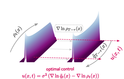
Figure 1: Schematic of forward and time-reversed probability flows for deriving state- and time-dependent dynamical interventions $u(x,t)$. We initially sample the flow $\varrho_{t}(x)$ for the time interval $[0,\,T]$. By employing the logarithmic gradient (score) of $\varrho_{t}(x)$, we evolve the time-reversed constrained probability flow $\tilde{q}_{t}(x)$. The optimal state- and time-dependent dynamical interventions $u(x,t)$ result from the difference of the logarithmic gradients of the two probability flows.

The new formulation of the optimal drift still requires the logarithmic gradient of the constrained flow $q_{t}(x)$, and therefore does not allow for direct simulation of controlled paths. Yet, this formulation of the optimal drift turns Eq.(14) into an equation resembling a Fokker–Planck equation, but with a negative diffusion term

$$\frac{\partial q_{t}(x)}{\partial t}=\nabla\cdot\Bigg{[}\Big{(}\sigma^{2}\nabla\ln\varrho(x,t)-f(x,t)\Big{)}q_{t}(x)\Bigg{]}-\frac{\sigma^{2}}{2}\nabla^{2}q_{t}(x).$$ (16)

However, by introducing the backward time variable ${\tau=T-t}$, and setting $\tilde{q}_{\tau}(x)=q_{T-\tau}(x)$ we obtain a new Fokker–Planck equation with properly signed diffusion

$$\frac{\partial\tilde{q}_{\tau}(x)}{\partial\tau} =-\nabla\cdot\Bigg{[}\Big{(}\sigma^{2}\nabla\ln\varrho_{T-\tau}(x)-f(x,T-\tau)\Big{)}\tilde{q}_{\tau}(x)\Bigg{]}$$ (17)

$$+\,\,\frac{\sigma^{2}}{2}\nabla^{2}\tilde{q}_{\tau}(x),$$

with initial condition $\tilde{q}_{0}(x)\propto\varrho_{T}(x)\chi(x)$.

Hence, we have represented the optimal control

$$u^{*}(x,t)=\sigma^{2}\Big{(}\nabla\ln\tilde{q}_{T-t}(x)-\nabla\ln\varrho_{t}(x)\Big{)},$$ (18)

as the difference of the logarithmic gradients of two forward probability flows ( score–functions ).

Hence, we have represented the optimal control

$$u^{*}(x,t)=\sigma^{2}\Big{(}\nabla\ln\tilde{q}_{T-t}(x)-\nabla\ln\varrho_{t}(x)\Big{)},$$ (19)

as the difference of the logarithmic gradients of two forward probability flows (score–functions). This result suggests a possible numerical strategy for obtaining the optimal interventions: First, solve the forward filtering equation for $\varrho_{t}(x)$ (Eq. (11)) using e.g. a particle filtering approach. Then approximate the logarithmic gradients $\nabla\ln\varrho_{T-\tau}(x)$ based on a sufficiently large number of stochastic particle paths. After this, simulate a number of random trajectories of the SDE which corresponds to the Fokker–Planck equation (Eq. (17)) and use the trajectories to approximate the score $\nabla\ln\tilde{q}_{T-t}(x)$. In fact, a similar approach was recently used to solve so–called Schrödinger bridge problems [67]. The latter can be also be understood as specific control problem for SDEs with only control energy costs (i.e. $U(x)\equiv 0$ and $\chi(x)=1$) in the cost functional (Eq.(7)), but in addition the probability densities $q_{0}(x)$ and $q_{T}(x)$ at initial and final times are specified as extra constraints. In contrast to these approaches, we apply and generalise a recent deterministic, particle framework for solving Fokker–Planck equations introduced by the authors in [52] to solve generic path integral control problems of the type of Eq. (7). This new technique avoids stochastic path sampling and reduces significantly temporal fluctuations, delivering thereby accurate Fokker–Planck equation solutions for relatively low number of employed particles [52]. In addition, the computation of the logarithmic gradients is already an integral part of the method for computing the deterministic particle dynamics.

.3 Deterministic particle flow (DPF) control

To sample the forward densities $\varrho_{t}(x)$ and $\tilde{q}_{t}(x)$, we build on the idea that a Fokker–Planck equation can be rewritten as a Liouville equation [68] for an ensemble of deterministic dynamical systems where the logarithmic gradient of the ensemble density acts as an additional force. In particular, for an SDE with drift $f(x,t)$ and diffusion $\sigma$, we rewrite the Fokker–Planck equation (Eq.(1)) for the probability density $p_{t}(x)$ of the system state in the form (see [52] for details)

$$\frac{\partial p_{t}(x)}{\partial t}=-\nabla\cdot\left[\left(f(x,t)-\frac{\sigma^{2}}{2}\nabla\ln p_{t}(x)\right)p_{t}(x)\right].$$ (20)

For a known density $p_{t}(x)$, this equation describes the evolution of an ensemble of independent systems with each ensemble member following the deterministic dynamics:

$$\frac{d{X}_{t}}{dt}=f({X}_{t},t)-\frac{\sigma^{2}}{2}{\nabla}\ln p_{t}({X}_{t}).$$ (21)

Note that here individual trajectories $X_{0:T}$ are distinct from solutions of the underlying SDE, since each ensemble individual follows pure deterministic dynamics.

To obtain a solution of the Fokker–Planck equation, we approximate the density $p_{t}(x)$ by an empirical distribution of $N$ ensemble members (’particles’) $\{X_{t}^{(i)}\}_{i=1}^{N}$ via

$$\hat{p}_{t}(x)\approx\frac{1}{N}\sum_{i=1}^{N}\delta\left(x-X_{t}^{(i)}\right).$$ (22)

Based on this empirical representation of the density $p_{t}(x)$, we approximate its logarithmic gradient with a statistical estimator $\hat{\nabla}\ln\hat{p}_{t}(X^{(i)}_{t})$, obtained from the solution variational formulation of the score function (see Supplementary Information). Thus, we express the resulting dynamics of individual particles in terms of a system of ordinary differential equations (ODEs)

$$\frac{dX^{(i)}_{t}}{dt}=f(X^{(i)}_{t},t)-\frac{\sigma^{2}}{2}\hat{\nabla}\ln\hat{p}_{t}(X^{(i)}_{t}).$$ (23)

While this approach is sufficient to solve control problems without path costs ($U(x,t)\equiv 0$), the extra sink term $-U(x,t)\varrho_{t}(x)$ in the forward filtering PDE (Eq.(11)) in the presence of path constraints requires an additional numerical technique. Thus, to incorporate path costs, we employ the formulation of the two stage process given by Eq.(12), and combine our Fokker-Planck deterministic particle solver with a deterministic particle filter method, the ensemble transform particle filter [66]. To simulate such a two stage process for each small time interval $\delta t$, we first propagate the particles following the dynamics of Eq.(23) to auxiliary positions $Y^{(i)}_{t}$ and assign to each particle $i$ a weight $\Omega_{i}$

$$\Omega_{i}(t)\propto e^{-\delta tU(Y^{(i)}_{t},t)}.$$ (24)

To transform the weighted particles to unweighted ones, we employ the ensemble transform particle filter [66]. This method solves an Optimal Transport [69] problem to provide the minimal necessary deterministic shifts required to transform an ensemble of weighted particles into an ensemble of uniformly weighted ones, by maximising the covariance between the two ensembles (see Supplementary Information).

.4 Guiding probability flows to extreme terminal states

In settings where the terminal target state lies outside of the typical values of the uncontrolled system, the sampled forward flow $\varrho_{t}(x)$ fails to provide sufficient evidence in the vicinity of the terminal point. Thereby the ensuing logarithmic gradient estimation $\nabla\log\varrho_{t}(x)$ is inaccurate.

For conservative systems and for terminal constraints defined by a delta function, i.e. $\chi(x)=\delta(x-x^{*})$, we address this issue by proposing an additional modified forward sampling that incorporates the extreme terminal constraint in the forward dynamics. To that end, we employ a $d$-dimensional Brownian Bridge (BB) dynamics. Brownian bridges are essentially Brownian motions, i.e. diffusions with vanishing drift $f(x)\equiv 0$, with a fixed terminal state $x^{*}$ (see Supplementary Information).

To maintain the correct path statistics, we employ the Girsanov’s change of measure formula to reweight the biased forward paths. More precisely, we obtain the correct path probability measure of the controlled process $\mathbb{P}^{BB}_{f}$ by reweighting the Brownian bridge path measure $\mathbb{P}^{BB}_{0}$ with the likelihood (Supplementary Information)

$$\frac{d\mathbb{P}^{BB}_{f}}{d\mathbb{P}^{BB}_{0}}(X_{0:T})\propto\exp\left[-\int_{0}^{T}U_{BB}(X_{t})dt\right],$$ (25)

with

$$U_{BB}(x)=\frac{1}{2\sigma^{2}}\left(f^{2}(x)+\sigma^{2}\nabla\cdot f(x)\right).$$ (26)

Hence, to simulate constrained paths of an SDE with drift $f(x)$ and extreme terminal constraints, we transform the extreme terminal constraint to a path constraint $U_{BB}(x)$ for an appropriate Brownian bridge process that already incorporates the terminal state $x^{*}$. In particular, we employ the modified forward equation

$$\frac{\partial\varrho_{t}(x)}{\partial t}={\cal{L}}_{f_{0}}\varrho_{t}(x)-U_{BB}(x)\varrho_{t}(x),$$ (27)

that generates paths with correct statistics that reach the terminal target by imposing the path constraint $U_{BB}(x)$ to the Brownian bridge forward dynamics with drift $f_{0}$. We term this variant of our framework guided Deterministic Particle Flow (gDPF) control.

Evaluation of optimal dynamical interventions

To illustrate our formalism in action, we computed optimal intervention protocols for biological systems by employing the proposed deterministic particle framework, and compared the obtained controls to those computed with the Path integral cross entropy method (PICE) (see Supplementary Information and  [44]). We tested our method on systems of increasing complexity and dimensionality, with conservative and non-conservative forces, as well as in settings with terminal, path, or collective state constraints.

To design the optimal interventions $u(x,t)$ we employed the presented method in two alternative variants: $i)$ the deterministic particle flow control (DPF), where the forward density follows the dynamics of Eq. (11), and $ii)$ the guided deterministic flow control (gDPF), in which the forward density evolves according to an appropriately reweighted Brownian bridge dynamics, as described in Section .4.

To evaluate the quality of the obtained controls, we considered the design of optimal interventions for artificially manipulating molecular phenotypes on adaptive landscapes (Section .6), for inducing state transitions to multistable conservative and non-conservative systems (Section .5), and for synchronising finite-size networks of Kuramoto phase oscillators (Section .7). We quantified the quality of the identified interventions in terms of employed control energy ($\|u(x,t)\|^{2}_{2}$), reflecting the optimality of the computed control, as well as in terms of deviations from terminal ($(x^{*}-X_{T})^{2}$) and path constraints ($U(X_{t},t)$), characterising thereby the effectiveness of the devised interventions to enforce the intended constraints. Unless explicitly mentioned otherwise, all metrics were evaluated by considering $1000$ independent stochastic trajectories controlled with each method.

.5 Controlling state transitions of conservative and non-conservative systems.

\begin{overpic}[width=433.62pt]{figs/Adouble_well_typical_backward_flows.png} \put(-1.0,21.0){\color[rgb]{0,0,0}{\Large{ a.}}} \put(24.0,21.0){\color[rgb]{0,0,0}{\Large{ b.}}} \put(48.0,21.0){\color[rgb]{0,0,0}{\Large{ c.}}} \put(71.0,21.0){\color[rgb]{0,0,0}{\Large{ d.}}} \end{overpic}

\begin{overpic}[width=433.62pt]{figs/Adouble_well_extreme_backward_flows.png} \put(-1.0,21.0){\color[rgb]{0,0,0}{\Large{ e.}}} \put(24.0,21.0){\color[rgb]{0,0,0}{\Large{ f.}}} \put(48.0,21.0){\color[rgb]{0,0,0}{\Large{ g.}}} \put(71.0,21.0){\color[rgb]{0,0,0}{\Large{ h.}}} \end{overpic}

Figure 2: Equivalence of dynamical interventions delivered by deterministic particle flow control (DPF), guided deterministic particle flow control (gDPF), and PICE, for typical (upper) and extreme (lower) terminal conditions. (upper) (a.) Controlled trajectories simulated by employing dynamical interventions delivered by deterministic particle flow control (magenta), guided deterministic particle flow control (orange), and path integral cross entropy method (grey). All trajectories started from initial point $x_{0}=-1$ (left silver circle) and reached the target $x^{*}=0$ at time $T=1$. (b.) Transient mean $\mu_{t}$ and standard deviation $\sigma_{t}$ over $1000$ independent trajectories controlled with each framework.(c.) Total control energy $\|u(x,t)\|^{2}$, and (d.) deviation from terminal point for $1000$ independent controlled trajectories with interventions computed according to each framework. Grey horizontal lines in (c.) and (d.) denote mean values over all realisations. The proposed methods result in slightly more expensive control costs, but are more consistent in precisely reaching the terminal state. (lower) Same as upper row for target $x^{*}=1$ only for gDPF and PICE. Here DPF is not applicable since the forward probability flow does not reach the extreme target point $x^{*}=1$.

We employed the proposed framework to devise interventions that reliably induced switching between stable states in a time constrained scheme for an one-dimensional conservative system and for a two-dimensional non-conservative one. For both settings, the unconstrained system either performs the state transition in a time unreliable way, or completely fails to reach the target, when the transition paths to that state strongly deviate from typical trajectories (Figure 2).

For the one-dimensional bistable system ($f(x)=4\,x-x^{3}$) starting from the stable state at $x_{0}=-1$, we provided optimal interventions under the objective of driving the system towards a predefined target $x^{*}$ at time $T=1$. We applied both variants of the presented method (DPF (Section .3) and gDPF (Section .4)), and explored two complementary scenarios: one with typical, $x^{*}=0$ (Figure 2a.-d.), and one with extreme, $x^{*}=1$ (Figure 2e.-h.), target states for the uncontrolled system at time $T$. Notice that the state $x^{*}=0$ is unstable, but outside of the basin of attraction of the initial state $x_{0}$.

Identified interventions successfully drive the system to target states. For the typical target state $x^{*}=0$, all three employed methods (DPF: magenta, gDPF: yellow, PICE: grey) successfully biased the controlled system towards the target $x^{*}$ (Figure 2a.). In fact, the distributions of simulated independent controlled trajectories delivered by each framework completely agreed throughout the entire time interval $[0,\,T]$ (Figure 2b.).

Considering the control energy dissipated by each method, DPF, on average, provided slightly larger interventions (Figure 2c.). Yet, both variants of our approach (DPF and gDPF) induced control trajectories that were consistently more exact in reaching the terminal state (Figure 2c.).

Comparing the distributions of terminal errors, DPF was both more accurate in reaching the target, as mediated by a smaller average value over the $1000$ realisations (grey bar), but also more precise, as indicated by the smaller dispersion of terminal errors around the average. This demonstrates that although DPF slightly overestimated the required controls, it provided sufficient force to lead the trajectories faithfully onto the target. In contrast, PICE relatively underestimated the necessary interventions, resulting in more energy efficient controls that nevertheless moderately deviated from the target.

Importantly, these results suggest that a single iteration of either variants of the proposed method (DPF or gDPF) provide comparable controls to the iterative PICE framework (grey).

For the extreme terminal state $x^{*}=1$, the guided probability flow deterministic control (gDPF) and the path integral cross entropy method (PICE) successfully pushed the system to the target (Figure 2e.)). The distributions of controlled trajectories (Figure 2f.) from the two frameworks showed complete agreement, while the control costs and terminal state precision were qualitatively similar to those obtained for the typical target state.

Notice that the deterministic particle flow control (DPF), the simple variant of our method, is inappropriate for this setting for a reasonable number of employed particles representing the forward flow. Since the target is an extreme system state for time $T$, it is highly unlikely that particles representing the forward flow $\varrho_{t}(x)$ will reach the target $x^{*}$. Thus the estimation of logarithmic gradients of the forward flow $\varrho_{t}(x)$ in the vicinity of the target will be inaccurate, since the particles will not provide sufficient evidence for gradient estimation in that region.

Departing from gradient systems, onward we consider triggering transitions between stable states in a time reliable way for a non-conservative system. To that end, we employed DPF for controlling a two dimensional phenomenological model of the function of a cell fate division module of a gene regulatory network [70] with self-excitation and cross inhibition (see Supplementary Information). We applied our method to induce transitions to the system between its co-existing stable states.

Similar to the conservative setting examined previously, the DPF successfully mediated the necessary interventions for the transition between the stable states (Figure 3 a.). We considered three noise conditions with $\sigma=\{1.,1.25,1.5\}$ and compared again the deterministic particle flow control (DPF) with the path integral cross entropy method (PICE). The transient statistics computed over $1000$ controlled trajectories for each framework agreed for all noise conditions (Figure 3b.) and Supplementary Information Figure).

Control costs and terminal error precision were comparable for the two approaches, with DPF performing slightly better in terms of dissipated control energy for increasing noise strength (Figure 3c.). Both methods had comparable control accuracy in reaching the target that deteriorated moderately for increasing noise amplitude. However, while DPF was considerable more accurate and precise for the low noise conditions, for larger noise amplitudes the accuracy of both methods in reaching the terminal point $x^{*}$ became comparable (Figure 3d.).

\begin{overpic}[width=433.62pt]{figs/systematic_non_conservative.png} \put(-1.0,23.0){\color[rgb]{0,0,0}{\Large{ a.}}} \put(24.0,23.0){\color[rgb]{0,0,0}{\Large{ b.}}} \put(49.0,23.0){\color[rgb]{0,0,0}{\Large{ c.}}} \put(73.0,23.0){\color[rgb]{0,0,0}{\Large{ d.}}} \end{overpic}

Figure 3: Optimal interventions effectively drive the non-conservative system to the target state for different noise amplitudes. (a.) Individual trajectory controlled by DPF (green-yellow) starting from stable state $\textbf{x}_{0}=(1.996,\,0.4)$ successfully reaches the target $\textbf{x}^{*}=(1,1)$ at $T=0.5$, while the uncontrolled trajectory (grey) fails to leave the basin of attraction of $\textbf{x}_{0}$. (b.) Agreement between controlled densities of $1000$ independent controlled trajectories driven by DPF (magenta) and PICE (grey) for noise amplitude $\sigma=1.5$. (c.) Dissipated control energy, and (d.) terminal error for increasing noise strength $\sigma$ for the two control frameworks. For increasing noise DPF delivers more efficient, but moderately less precise controls than PICE.

Taken together, DPF (and gDPF where necessary) successfully provided the necessary controls for reaching the targets in both conservative and non-conservative systems and under various noise conditions. The provided interventions where on par with the established iterative PICE framework in terms of dissipated control energy, and moderately more precise in reaching the target.

.6 Evolutionary control through artificial selection.

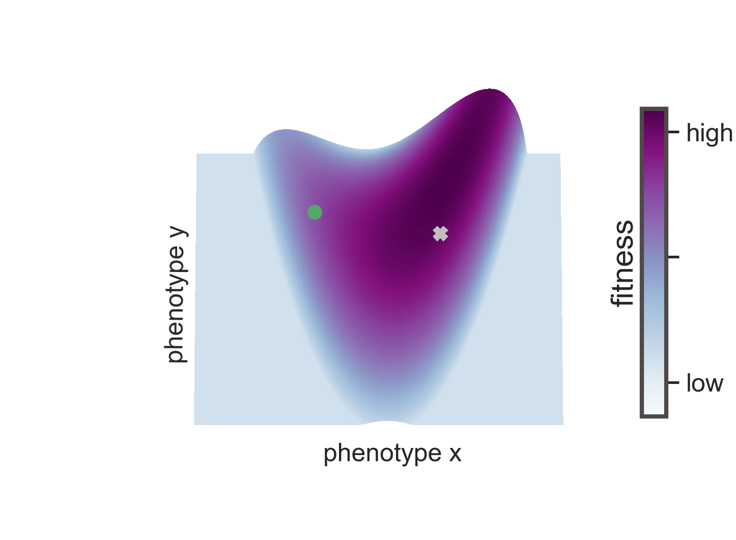
Figure 4: The phenotypic landscape .

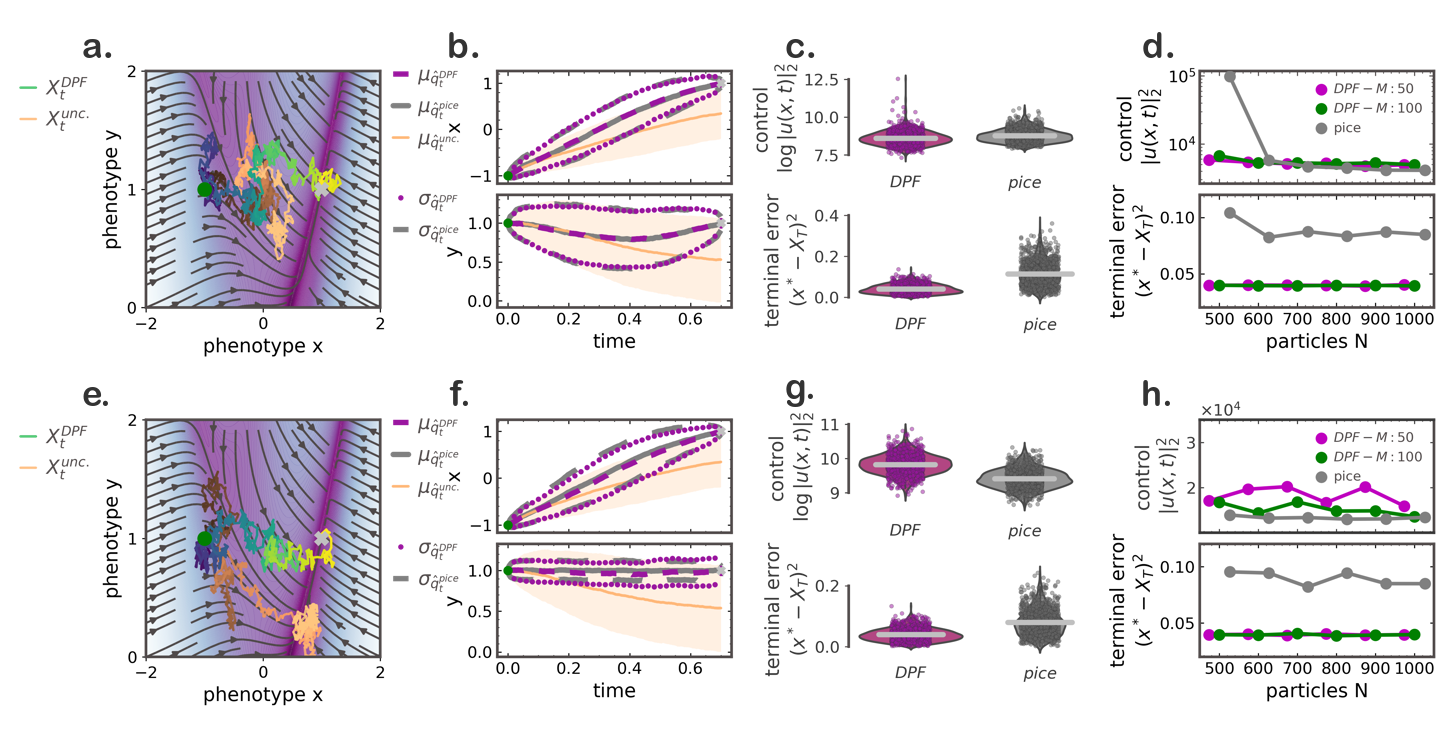
Figure 5: Deterministic particle flow (DPF) control provides optimal interventions to drive evolution to target state (grey cross). (a.) A controlled trajectory starting from phenotypic state $(-1,1)$ reaches the target state $(1,1)$ at time $T=0.7$ (blue-yellow line), while an uncontrolled trajectory remains in the vicinity of initial state during the same time interval (orange line). (b.) Mean and standard deviation of the marginal densities of $1000$ controlled trajectories employing interventions computed with our framework DPF (purple) and with PICE (grey). Orange line indicates mean of $1000$ uncontrolled trajectories, while shaded area captures the associated standard deviation. For estimating the controls we employed $N=400$ particles for DPF, and $N_{pice}=500$ for PICE. (c.) Comparison of (upper) (logarithmic) control energy $\|u(x,t)\|^{2}_{2}$, and (lower) deviation from the terminal point $\|X_{T}-x^{*}\|^{2}$ for each controlled trajectory with interventions computed according to DPF (magenta) and PICE (grey). (d.) (Logarithmic) control energy (upper) improves moderately, and terminal error (lower) remains constant for increasing particle number $N$. The number of inducing points in the logarithmic gradient estimation conveys negligible difference in control energy and terminal error (inducing point number magenta: $M=50$, green: $M=100$ ). Grey line indicates the performance of PICE in the same setting. (e.-h.) Same as (a.-d.) with additional path constraint $U((x,y),t)=(y-1)^{2}$.

Building upon the evolutionary stochastic control formalism recently introduced by Nourmohammad et. al [28], we employed deterministic particle flow control to devise artificial selection protocols for molecular phenotypes that optimally drive evolution to desired phenotypic states. In this setting experimentally imposed path constraints become relevant for preventing undesirable outcomes on covarying phenotypes.

For an evolving population, the main evolutionary drivers comprise fitness and mutation forces that continuously adjust the composition of phenotypes in the population, while genetic drift perturbs the whole process stochastically. We described the evolution of the mean phenotypes $\mathbf{dx}$ of the population by the overdamped Langevin equation [71]

$$d\mathbf{x}=C\cdot\nabla F(x)dt+\sigma d\mathbf{W},$$ (28)

with $F(x)$ denoting the adaptive fitness landscape in the presence of natural selection [72], and $\sigma$ the noise amplitude that rescales the genetic drift, i.e. the stochastic term, according to the population size $n$ and the covariance matrix $C$, $\sigma=C^{1/2}n^{-1}$ . The gradient of the landscape $f(x)=C\cdot\nabla F(x)$ captures the adaptive pressures under natural selection.

In contrast to commonly employed assumptions of spherically symmetric adaptive landscapes, to demonstrate the richness of our method and supported by empirical findings [73], we considered an asymmetric rugged landscape [74]. Such landscapes may arise in small sized populations with small variance and multi-modal fitness functions for each individual [75]. For simplicity we consider the covariance matrix $C$ constant, given the much smaller timescales upon which its fluctuations unfold [76], and its weak dependency on the evolutionary selection strength [77].

The dynamics of Eq.(28) describe the evolution of populations in the presence of natural selection towards an evolutionary optimum, captured by the maximum of the adaptive landscape, adhering thereby to physiological and environmental constraints.

To study the outcomes and dynamics of adaptive evolution, intervention protocols are required that drive phenotypes towards non-evolutionary optimum states $\mathbf{x^{*}}$, or through evolutionary trajectories that deviate from landscape gradients. These interventions are implemented through artificial selection, which, following [28], we formulate as a time- and state- dependent perturbation $\mathbf{u}(x,t)$ to the natural selection, and apply DPF to obtain the necessary controls.

Single-objective and multi-objective directed evolution. For a system with multiple covarying phenotypes evolving on the landscape $F(x,y)=((1-x)^{2}+(y-x^{2})^{2})$ (Figure 4), changes along one phenotypic axis are often accompanied by changes along covarying phenotypic traits as dictated by the landscape gradient. Thus attempts to bias and enhance selective forces towards a specific phenotype, may lead to undesired variations along the covarying traits. To demonstrate this, we controlled phenotypic trajectories initiated at state $\mathbf{x}_{0}=(-1,1)$ with target state $\mathbf{x}^{*}=(1,1)$. The designed interventions by DPF with only terminal constraints $\chi(\mathbf{x})=\delta(\mathbf{x}-\mathbf{x}^{*})$ successfully drove the system to the intended target (Figure 5a.-b.). Nevertheless, although the initial and terminal state along the second dimension remained the same, as expected, without introducing additional path constraints, the phenotypic trait along the second dimension ($y$) underwent considerable transient fluctuations as indicated by the non-constant mean of the simulated paths ($\mu_{\hat{q}_{t}}$), as well as by the increasing dispersion of paths from the mean, as captured by the standard deviation $\sigma_{\hat{q}_{t}}$ (Figure 5b.).

To limit the fluctuations along the covarying second phenotypic trait, we introduced path constraints

$$U((x,y),t)=10^{3}\,(y-1)^{2}$$

that penalised transient deviations from the intended value of the second trait $y$ (Figure 5e.). The necessary interventions, identified by DPF with path constraints, successfully controlled the system towards the predefined target, reducing thereby considerably the fluctuations along the second axis (Figure 5e. and f.). Compared to the path integral control framework (PICE), for both scenarios, our method delivered results with comparable dissipated control energy and considerably more precise in terms of terminal errors (Figure 5e. and f.).

Evaluating the performance of both methods for increasing particle number $N$ employed for the estimation of the required interventions $u(x,t)$, revealed that DPF provided controls on par with PICE already for $N=500$ particles and, by design, only with a single iteration. More precisely, the proposed method presented a relatively stable performance for increasing particle number, with small improvement in terms of exerted control energy, whereas the path integral cross entropy method improved substantially when more particles where employed in the computations, and consequently matched in performance our approach. Considering the deviation from the terminal state, DPF was consistently more precise and accurate in reaching the target as indicated both by considerably smaller terminal errors (Figure 5d. and h.), and by smaller deviations of individual terminal states around the average (Supplementary Figure 5). Both the exerted control energy and terminal error do not show considerable improvement for increasing inducing point number employed in the logarithmic gradient estimator (magenta for $M=50$; green for $M=100$).

.7 Controlling collective states: synchronisation control of stochastic Kuramoto oscillators

\begin{overpic}[width=433.62pt]{figs/Kuramoto_2N_trajectories.png} \put(2.0,28.0){\color[rgb]{0,0,0}{\Large{ a.}}} \put(34.0,28.0){\color[rgb]{0,0,0}{\Large{ b.}}} \put(66.0,28.0){\color[rgb]{0,0,0}{\Large{ c.}}} \end{overpic}

Figure 6: Synchronisation control of two coupled Kuramoto phase oscillators. (a.) Evolution of phases ($\theta_{i}$) of two controlled (purple) and two uncontrolled (green) Kuramoto oscillators mutually coupled with coupling $J=1.2$ and noise amplitude $\sigma=1.0$. (b.) Evolution of Kuramoto phase-coherence order parameter $R$ for the controlled (purple) oscillators indicates a fast transition to synchrony (R=1), while, the identical uncontrolled oscillators become progressively incoherent, indicated by a strongly fluctuating order parameter (green). The orange line denotes the expected long time average value of the order parameter for non-interacting oscillators considering finite size scaling effects. The grey line marks the level of $R=1$ indicating a completely synchronous state. (c.) Control input provided to each oscillator.

\begin{overpic}[width=433.62pt]{figs/Kuramoto_2.png} \put(2.0,50.0){\color[rgb]{0,0,0}{\Large{ a.}}} \put(44.0,50.0){\color[rgb]{0,0,0}{\Large{ b.}}} \end{overpic}

Figure 7: Synchronisation control a network of two coupled Kuramoto phase oscillators for different coupling strengths. (a.) Time averaged phase-coherence order parameter ($R$) of controlled (purple) and uncontrolled (green) networks under different noise conditions ($\sigma=0.5$ - triangles, $\sigma=1.0$ - circles). The proposed method (DPF) effectively synchronises the controlled oscillators already for vanishing coupling strength between them. (b.) Evolution of Kuramoto order parameter $R$ for networks with coupling $J=2.0$ and two noise conditions ($\sigma=0.5$ - (upper), $\sigma=1.0$ - (lower)) for controlled (purple) and uncontrolled (green) oscillators. The control induces fast transition to synchrony (R=1), while the identical uncontrolled oscillators either synchronise slower (for low noise), or become only partially synchronised (for strong noise). Individual lines indicate evolution of the order parameter in $20$ realisations of the network starting from same initial conditions and from a single computation of the required controls for each setting (where relevant). Dotted black lines denote the mean over the $20$ realisations.

\begin{overpic}[width=433.62pt]{figs/Kuramoto_2_onset.png} \put(5.0,35.0){\color[rgb]{0,0,0}{\Large{ a.}}} \put(52.5,35.0){\color[rgb]{0,0,0}{\Large{ b.}}} \end{overpic}

Figure 8: Onset of synchronisation and percentage of time in synchronised state after synchrony onset reveal the effectiveness of deterministic particle flow control to induce robust synchronisation on a network of $K=2$ oscillators . (a.) Onset of synchronisation for controlled (purple) and uncontrolled (green) networks quantified as the first time $t^{syn}$ the phase-coherence order parameter exceeds $R\geq 0.99$ and remains over that value for duration $\tau^{s}=20\times dt=0.02$ time units. Grey annotations denote the percentage of the examined networks that reached the synchronous state for duration $\tau^{s}$. Absence of annotation indicates that all examined networks reached synchrony. (b.) Percentage of simulation time the networks spontaneously spent in synchronised state ($R\geq 0.99$) after synchrony onset $t^{syn}$. Both figures consider two different noise conditions ($\sigma=0.5$ - triangles, $\sigma=1.0$ - circles).

To further demonstrate the generalisability of the proposed framework, we considered a system where the constraints do not explicitly penalise exact regions of the state space, but rather pertain the collective state of a system of interacting stochastic units. Specifically, we applied our method for synchronising finite size networks of stochastic Kuramoto phase oscillators (see Supplementary Information for details). We performed systematic studies on a prototypical network of two interacting oscillators (Fig. 6 , Fig. 5, and Fig. 6), and a network of $K=6$ (Fig. 8 and Fig. 10) heterogeneous oscillators with all-to-all uniform coupling (Supplementary Information).

\begin{overpic}[width=216.81pt]{figs/Kuramoto_6instance.png} \put(2.0,70.0){\color[rgb]{0,0,0}{\large{ a.}}} \put(47.0,70.0){\color[rgb]{0,0,0}{\large{ c.}}} \put(2.0,32.0){\color[rgb]{0,0,0}{\large{ b.}}} \put(47.0,32.0){\color[rgb]{0,0,0}{\large{ d.}}} \end{overpic}

Figure 9: Synchronisation control of a finite-size network of $K=6$ interacting Kuramoto phase oscillators. (a.) Evolution of phases $\theta$ of a controlled network, and (b.) an identical uncontrolled network. The phases of the oscillators quickly synchronise when controlled by DPF and remain synchronised throughout the entire simulation interval $[0,\,T=0.5]$. In the absence of control the phases of the oscillators become increasingly incoherent. (c.) Evolution of Kuramoto order parameter capturing phase coherence $R$ for the controlled (purple) oscillator network indicates a rapid transition to complete synchrony ($R=1$) for all $20$ realisations (individual purple lines). The order parameter of identical uncontrolled networks fluctuates strongly indicating partial incoherence (green). The orange line denotes the expected long time average value of the order parameter if the oscillators were non-interacting considering finite size scaling effects. For visual clarity, the grey line marks the level of $R=1$ indicating a completely synchronous state. (d.) Control energy spent on all $K=6$ oscillators for a single control realisation.

\begin{overpic}[width=433.62pt]{figs/systematic_Kuramoto_6N.png} \put(-1.0,50.0){\color[rgb]{0,0,0}{\Large{ a.}}} \put(44.5,50.0){\color[rgb]{0,0,0}{\Large{ b.}}} \end{overpic}

Figure 10: Synchronisation control of a network of six heterogeneous Kuramoto phase oscillators for different coupling strengths. (a.) Time averaged phase-coherence order parameter ($R$) of controlled (purple) and uncontrolled (green) networks under different noise conditions ($\sigma=1.0$ - triangles, $\sigma=1.5$ - circles). The proposed method (DPF) effectively synchronises the controlled oscillators already for weak coupling. (b.) Evolution of Kuramoto order parameter $R$ for networks with coupling $J=3.0$ and two noise conditions ($\sigma=1.0$ - (upper), $\sigma=1.5$ - (lower)) for controlled (purple) and uncontrolled (green) oscillators. The control induces fast transition to synchrony ($R=1$), while the identical uncontrolled oscillators either synchronise slower (for low noise), or become only partially synchronised (for strong noise). Individual lines indicate evolution of the order parameter in $20$ realisations of the network starting from same initial conditions and from a single computation of the required controls for each setting (where relevant). Dotted black lines denote the mean over the $20$ realisations.

To accommodate synchronisation control with our framework, we considered a time constrained setting where we applied DPF for an interval $[0,\,T]$ (time units). An alternative ’online’ approach described in the Supplementary Information alternates computation of controls within small time intervals with simulation of controlled trajectories over those intervals.

We implemented the synchronisation constraint as a path constraint that promotes synchrony without any further requirement for the terminal state, and characterised the level of synchronisation in terms of the Kuramoto order parameter for phase coherence $R(\bm{\theta},t)$ (Supplementary Information)

$$R(t)=\frac{1}{K}|\sum^{K}_{j=1}e^{i\theta_{j}(t)}|.$$ (29)

To that end, we employed the following path constraint that promotes order parameter values closer to $1$, i.e. closer to a synchronous state

$$\mathcal{U}(\bm{\theta}_{t})=\beta\left(1-R(\bm{\theta}_{t},t)\right)dt,$$

with $\bm{\theta}_{t}\in\mathbb{R}^{K}$ denoting the vector of oscillator phases, and $\beta\in\mathbb{R}$ a scaling constant.

For all considered networks of interacting Kuramoto oscillators we applied interventions $u_{i}(\bm{\theta}_{t},t)$ on the phases ${\bm{\theta}=\{\theta_{i}\}^{K}_{i=1}}$ of all network nodes. Further considerations of optimally selecting a subset of nodes to control were out of the scope of the current article.

For a prototypical network of $K=2$ interacting oscillators with weak coupling ($J=1.2$), DPF induced rapid synchrony, whereas the uncontrolled oscillators became progressively incoherent as indicated both by observing their phases (Figure 6a.) and the transient values of their phase-coherent order parameter $R$ (Figure 6b.). DPF provided fairly strong control inputs at the beginning of the simulation to fully align the phases of the oscillators (Figure 6c.), and subsequently delivered only moderate controls to maintain synchrony counteracting the effect of noise.

DPF successfully induced synchrony for different levels of coupling and under two different noise conditions ${\sigma=\{0.5,1.0\}}$ (Figure 5a.). For strongly coupled oscillators where the uncontrolled network progressively synchronises solely due to the interactions, DPF synchronised the oscillators faster - indicated by earlier reaching the order parameter ${R=1}$ value compared to their uncontrolled counterparts - and prevented spontaneous desynchronsation events that occurred in the uncontrolled networks especially in the presence of strong noise (Figure 5b.).

To quantify these effects further, we analysed the onset of synchronisation $t^{syn}$ and the percentage of time spent in the synchronised state of the examined controlled and uncontrolled networks for increasing coupling $J$.

For each network realisation, we defined the onset of synchronisation $t^{syn}$ as the first time point when the phase-coherence order parameter exceeded the value $R\geq 0.99$ and remained above that value for a minimal duration of $\tau^{s}=20\times dt=0.02$ time units. For uncontrolled networks with weak couplings we considered only the subset of realisations that reached the synchronous state (indicated as a ratio by the grey annotations in Figure 6a.). To quantify the robustness of synchronisation in each network, we estimated the percentage of time the network remained synchronised after the synchronisation onset by counting the time points when the order parameter spontaneously exceeded the $R=0.99$ threshold after $t^{syn}$.

For both noise conditions and independent of coupling strength $J$, networks controlled by DPF reached the synchronous state considerably faster than their uncontrolled counterparts (Figure 6a.), and consistently remained synchronised for the entire simulation, as mediated by the percentage of time spent in the synchronised state after the synchronisation onset $t^{syn}$. More precisely, while a subset of uncontrolled weakly coupled networks synchronised for at least $\tau^{s}=20$ time units, as expected due to the presence of noise they failed to remain in that synchronised state as indicated in Figure 6b. For stronger couplings desynchronisation was less pronounced, yet still more frequent than in their controlled counterparts.

For $K=6$ interacting heterogeneous oscillators and for network charachteristics (coupling strength $J=1.$ and noise amplitude $\sigma=1.0$) that render the uncontrolled system only partially synchronisable (Figure  8 b.(lower)), state feedback control delivered by DPF successfully drove the oscillators to a fully synchronised state (Figure  8 b.(upper)). As indicated by the evolution of the Kuramoto order parameter for each of the $20$ realisations shown in Figure  8 b., our framework not only delivered sufficient controls to rapidly synchronise the oscillators, but also provided the necessary interventions to maintain the phase synchronisation (Figure  8 c.). In fact, as indicated by the non-fluctuating order parameter $R$ for most realisations, only $2$ network instances underwent spontaneous noise-induced desynchronisations late in the simulations, which nevertheless were partially recovered.

Similar to the smaller network, the six oscillator network was successfully synchronised for a range of coupling strengths (Figure 10a.) and for both noise conditions. Compared to the identical uncontrolled networks, the networks controlled by DPF exhibited consistently larger order parameter values. Although some networks underwent spontaneous desynchronisations, these were quickly efficiently recovered (Figure 10b.).

Discussion

In this work, we introduced a novel methodological framework for identifying optimal dynamical interventions for constraining diffusive systems. Distinctively from previous work [26, 44, 27, 78] that devises optimal control protocols by employing iterative optimisation procedures, here, we obtained the required interventions in a deterministic and non-iterative way. In particular, we showed that splitting the time-resolved constraining information into retrospective and prospective parts, allows for a representation of the optimal interventions in terms of the difference of logarithmic gradients (scores) of two forward probability flows. By introducing statistical estimators for the logarithmic gradients of the empirical probability densities, and by employing novel advances for deterministic evolution of sample based probability flows [52, 66], we proposed an efficient, non-parametric approximation of the optimal controls.

We demonstrated the feasibility and potential of our framework on a battery of diverse biologically inspired systems and challenging settings of increasing complexity and dimensionality. More precisely, we employed the proposed deterministic particle flow control (DPF) to induce switches between stable states on multi-stable systems (Section .5), to devise artificial selection protocols on phenotypic landscapes by implementing constraints for co-varying phenotypes (Section .6), and to induce synchronisation on networks of stochastic phase oscillators.

We compared our approach against the recently proposed Path integral cross entropy method [44], which approximates time dependent controls by an iterative optimisation based on stochastic path sampling. Our results suggest that our one-shot, deterministic framework is on par with the iterative path integral cross entropy method in terms of control efficiency, and more precise and accurate in terms of deviation from terminal target states.

Moreover, through the nonparametric estimation of the logarithmic gradients, our method is inherently model agnostic, being able, in principle, to approximate the logarithmic gradient of arbitrary distributions, and therefore estimate external interventions of arbitrary functional form. In turn, the path integral cross entropy method requires an a priori selection of the number of basis functions employed in the approximation, implicitly constraining the class of control functions that may be implemented. In fact, inappropriate choice of basis function parameters results in numerical instabilities in the form of non converging matrix inversions and diverging trajectories during the optimisation, before the algorithm converges to an optimum. We found that this effect could not be mitigated by adjusting the learning rate or other parameters to smaller values. The trade off, however, pertains the nature of our approximation, which as a kernel method, is more expensive compared to basis functions during the actual evaluation of the identified controls.

In this work, we propagated probability densities by employing recent advances for solving Fokker–Planck equations in terms of deterministic particle dynamics. However, in principle, any particle filtering algorithm employing stochastic particle dynamics may be combined with the logarithmic gradient density estimator to obtain a numerical approximation of the time-reversed drift of Eq. (19) at each time step. Numerical experiments of such a method showed, that the stochastic fluctuations of the particles lead to fairly noisy control estimates over time. Hence, here, taking advantage of the fact that the deterministic sampling framework of  [52] already employs the logarithmic gradient estimator as a building block, we integrated this method into the computation of the optimal interventions.

Although the representation of constrained densities with particles is computationally more efficient compared to solutions of discretised PDEs, control representations for regions of the state space where the particles do not provide sufficient evidence for the underlying density, will be inaccurate. While the probability density functions for the regions of the state space unoccupied by particles are expected to have vanishing values, with inadequate number of particles, the estimated logarithmic gradient of the related densities might be inaccurate in those regions. Yet, due to the deterministic nature of our approach, our framework provides better representation of the underlying densities compared to a pure stochastic path sampling.

We expressed the optimal interventions as a time and space dependent perturbation of the uncontrolled dynamics that are obtained from the logarithmic gradient of a backward PDE. This formulation results from linearising the Hamilton-Jacobi-Bellman equation (Supplementary Information). An equivalent formulation for optimal drift adjustment for constraining diffusion processes has been derived in the field of statistical mechanics by applying the Doob’s $h$-transform [79, 80, 81, 64, 22]. This formulation agrees with the one employed here in the absence of path constraints. In that case, the optimal interventions may be obtained from the logarithmic gradient of the solution of the backward Kolmogorov equation. However, the solution of the backward Kolmogorov equation is known in closed form only for trivial systems, may be cumbersome to obtain for general multidimensional systems, while the ensuing computation of the logarithmic gradient of the solution may run into numerical instabilities . Here, by representing the densities with particles, and by directly estimating the logarithmic gradients of the particle density, we provided an efficient and feasible solution for obtaining the necessary drift adjustments.

The present work proposes a method for controlling stochastic systems by manipulating their dynamical variables. However, often such a scenario might be insufficient. Interventions in biological systems may have limited access to the the system’s state variables, or only system parameters might be accessible for control. In these settings, an extension of the path integral control framework that additionally considers the system parameters is required. Existing methods that consider parameter optimisation are limited to properly function only in weak noise settings [27] due to large deviations arguments employed in their derivation.

We successfully employed the proposed method for synchronisation control of networks of coupled stochastic Kuramoto oscillators. However, when path constraints are required, the DPF solves an optimal transport problem at every time step to implement the path constraints as a deterministic particle resampling. This computation employs the Earth Mover’s distance (EMD) for an ensemble of $N$ particles, which scales rather unfavorably for increasing particle number as $\mathcal{O}(N^{3}\log N)$. Here, for the networked systems that required large number of particles, we employed an alternative solution for computing the EMD, the network simplex solver [82, 83], which has computational complexity that scales as $\mathcal{O}(N^{2})$, providing thereby a considerable speedup in the calculations. Yet, we still consider this necessary particle shifting a computational bottleneck for our framework. Future developments will focus on incorporating this step into the forward particle dynamics and thus will scale more favourably with particle number, enabling thereby the control of systems of higher dimensionality.

Moreover, considering the topic of network synchronisation, we considered out of the scope of the present paper to explore the possibility of controlling only a subset of network nodes. Previous attempts to solve the same problem in a stochastic setting have considered only the synchronisation of two coupled identical Kuramoto oscillators [84], while, here, we considered networks up to six oscillators with differing natural frequencies. Insights from network control theory for nonlinear systems coupled with the proposed framework may provide a more control-energy efficient approach for network synchronisation. Additionally, further systematic studies that will explore various network topologies, coupling schemes, and intrinsic parameter heterogeneities, will provide additional insight on the properties of our method to induce robust synchronisation to networks of interacting stochastic phase oscillators.

The proposed framework is further relevant for several computational or applied settings, where marginal densities of constrained diffusive systems are required, i.e. for state estimation of such systems between two successive state observations, or for computing the transition probabilities in extreme event calculations. In those settings, only the constrained path distribution $q_{t}(x)$ is required instead of the precise dynamical interventions. Although not explicitly demonstrated here, DPF is also applicable for computing averages over constrained densities or functionals over constrained paths. Since the reverse time sampled flow $\tilde{q}_{t}(x)$ already provides a good representation of the constrained density, averages over functions evaluated on the paths of $q_{t}(x)$ already provide accurate estimates of the computed quantities.

More broadly, the field of simulation based inference [85, 86] has developed dramatically in the past years due to expanding computational capacities offered by current computing devises able to simulate models considered demanding in the past. These methods perform inference for models with intractable likelihoods (like sparsely observed stochastic systems) requiring frameworks for accurate and efficient simulation of detailed dynamical models that provide dynamical trajectories of candidate models to perform inference. Thereby, our approach, by providing direct samplings of dynamically constrained diffusion processes will enable efficient inference of such systems.

We employed the proposed framework on a prototypical scenario of devising artificial selection protocols for molecular phenotypes inspired by  [28]. The nascent field of continuous culturing [87, 88] for studying adaptive evolution has created a growing demand for devising efficient and precise stochastic control frameworks that may be integrated in advanced open-source continuous culturing platforms like eVOLVER [29] to manipulate and control cell culture growth and phenotyping. These platforms enable real time monitoring of cell cultures and administer exact custom perturbations in the form of selection pressures, or by adjusting the constant nutrient feed input to the culture. By providing accurate interventions that implement arbitrary state constraints the proposed DPF control is suitable to be integrated in such a platform.

The clearest advantage of our framework is its non-iterative, non-parametric, and deterministic nature, providing thereby computational advantages compared to existing control methods [44, 89]. Moreover, the proposed formulation for the optimal interventions generalises beyond particle systems and may be easily implemented by neural networks.

References

- Raser and O’shea [2005] Jonathan M Raser and Erin K O’shea. Noise in gene expression: origins, consequences, and control. Science, 309(5743):2010–2013, 2005.
- Swain et al. [2002] Peter S Swain, Michael B Elowitz, and Eric D Siggia. Intrinsic and extrinsic contributions to stochasticity in gene expression. Proceedings of the National Academy of Sciences, 99(20):12795–12800, 2002.
- Hasty et al. [2000] Jeff Hasty, Joel Pradines, Milos Dolnik, and James J Collins. Noise-based switches and amplifiers for gene expression. Proceedings of the National Academy of Sciences, 97(5):2075–2080, 2000.
- Kepler and Elston [2001] Thomas B Kepler and Timothy C Elston. Stochasticity in transcriptional regulation: origins, consequences, and mathematical representations. Biophysical journal, 81(6):3116–3136, 2001.
- García-Ojalvo and Sancho [2012] Jordi García-Ojalvo and José Sancho. Noise in spatially extended systems. Springer Science & Business Media, 2012.
- Eldar and Elowitz [2010] Avigdor Eldar and Michael B Elowitz. Functional roles for noise in genetic circuits. Nature, 467(7312):167–173, 2010.
- Simpson et al. [2009] Michael L Simpson, Chris D Cox, Michael S Allen, James M McCollum, Roy D Dar, David K Karig, and John F Cooke. Noise in biological circuits. Wiley Interdisciplinary Reviews: Nanomedicine and Nanobiotechnology, 1(2):214–225, 2009.
- Blake et al. [2003] William J Blake, Mads Kærn, Charles R Cantor, and James J Collins. Noise in eukaryotic gene expression. Nature, 422(6932):633–637, 2003.
- Horsthemke [1984] Werner Horsthemke. Noise induced transitions. In Non-equilibrium dynamics in chemical systems, pages 150–160. Springer, 1984.
- Zhou et al. [2005] Tianshou Zhou, Luonan Chen, and Kazuyuki Aihara. Molecular communication through stochastic synchronization induced by extracellular fluctuations. Physical Review Letters, 95(17):178103, 2005.
- Del Vecchio et al. [2016] Domitilla Del Vecchio, Aaron J Dy, and Yili Qian. Control theory meets synthetic biology. Journal of The Royal Society Interface, 13(120):20160380, 2016.
- Nguyen et al. [2021] Phuc Nguyen, Nicholas A Pease, and Hao Yuan Kueh. Scalable control of developmental timetables by epigenetic switching networks. Journal of the Royal Society Interface, 18(180):20210109, 2021.
- Sivak and Crooks [2012] David A Sivak and Gavin E Crooks. Thermodynamic metrics and optimal paths. Physical Review Letters, 108(19):190602, 2012.
- Zulkowski et al. [2012] Patrick R Zulkowski, David A Sivak, Gavin E Crooks, and Michael R DeWeese. Geometry of thermodynamic control. Physical Review E, 86(4):041148, 2012.
- Gomez-Marin et al. [2008] Alex Gomez-Marin, Tim Schmiedl, and Udo Seifert. Optimal protocols for minimal work processes in underdamped stochastic thermodynamics. The Journal of chemical physics, 129(2):024114, 2008.
- Rabitz et al. [2000] Herschel Rabitz, Regina de Vivie-Riedle, Marcus Motzkus, and Karl Kompa. Whither the future of controlling quantum phenomena? Science, 288(5467):824–828, 2000.
- Pechen and Tannor [2011] Alexander N Pechen and David J Tannor. Are there traps in quantum control landscapes? Physical Review Letters, 106(12):120402, 2011.
- Hendrix and Jarzynski [2001] DA Hendrix and C Jarzynski. A “fast growth” method of computing free energy differences. The Journal of Chemical Physics, 114(14):5974–5981, 2001.
- Shirts et al. [2003] Michael R Shirts, Eric Bair, Giles Hooker, and Vijay S Pande. Equilibrium free energies from nonequilibrium measurements using maximum-likelihood methods. Physical Review Letters, 91(14):140601, 2003.
- Schmiedl and Seifert [2007] Tim Schmiedl and Udo Seifert. Optimal finite-time processes in stochastic thermodynamics. Physical Review Letters, 98(10):108301, 2007.
- Hartmann and Schütte [2012] Carsten Hartmann and Christof Schütte. Efficient rare event simulation by optimal nonequilibrium forcing. Journal of Statistical Mechanics: Theory and Experiment, 2012(11):P11004, 2012.
- Chetrite and Touchette [2015] Raphaël Chetrite and Hugo Touchette. Variational and optimal control representations of conditioned and driven processes. Journal of Statistical Mechanics: Theory and Experiment, 2015(12):P12001, 2015.
- Kim and Mehta [2020] Jin Won Kim and Prashant G Mehta. An optimal control derivation of nonlinear smoothing equations. In Proceedings of the Workshop on Dynamics, Optimization and Computation held in honor of the 60th birthday of Michael Dellnitz, pages 295–311. Springer, 2020.
- Casadiego et al. [2018] Jose Casadiego, Dimitra Maoutsa, and Marc Timme. Inferring network connectivity from event timing patterns. Physical review letters, 121(5):054101, 2018.
- Todorov [2009] Emanuel Todorov. Efficient computation of optimal actions. Proceedings of the National Academy of Sciences of the United States of America, 106(28):11478–11483, 2009.
- Kappen [2005a] Hilbert J Kappen. Linear theory for control of nonlinear stochastic systems. Physical Review Letters, 95(20):200201, 2005a.
- Wells et al. [2015] Daniel K Wells, William L Kath, and Adilson E Motter. Control of stochastic and induced switching in biophysical networks. Physical Review X, 5(3):031036, 2015.
- Nourmohammad and Eksin [2021] Armita Nourmohammad and Ceyhun Eksin. Optimal evolutionary control for artificial selection on molecular phenotypes. Physical Review X, 11(1):011044, 2021.
- Zhong et al. [2020] Ziwei Zhong, Brandon G Wong, Arjun Ravikumar, Garri A Arzumanyan, Ahmad S Khalil, and Chang C Liu. Automated continuous evolution of proteins in-vivo. ACS synthetic biology, 9(6):1270–1276, 2020.
- Kao et al. [2021] Ta-Chu Kao, Mahdieh S Sadabadi, and Guillaume Hennequin. Optimal anticipatory control as a theory of motor preparation: a thalamo-cortical circuit model. Neuron, 109(9):1567–1581, 2021.
- Iolov et al. [2014] Alexandre Iolov, Susanne Ditlevsen, and André Longtin. Stochastic optimal control of single neuron spike trains. Journal of Neural Engineering, 11(4):046004, 2014.
- Scott [2004] Stephen H Scott. Optimal feedback control and the neural basis of volitional motor control. Nature Reviews Neuroscience, 5(7):532–545, 2004.
- Bernton et al. [2019] Espen Bernton, Jeremy Heng, Arnaud Doucet, and Pierre E Jacob. Schrödinger Bridge Samplers. arXiv preprint arXiv:1912.13170, 2019.
- Vargas et al. [2021] Francisco Vargas, Pierre Thodoroff, Neil D Lawrence, and Austen Lamacraft. Solving Schrödinger Bridges via Maximum Likelihood. arXiv preprint arXiv:2106.02081, 2021.
- Exarchos and Theodorou [2018] Ioannis Exarchos and Evangelos A Theodorou. Stochastic optimal control via forward and backward stochastic differential equations and importance sampling. Automatica, 87:159–165, 2018.
- Song et al. [2020] Yang Song, Jascha Sohl-Dickstein, Diederik P Kingma, Abhishek Kumar, Stefano Ermon, and Ben Poole. Score-based generative modeling through stochastic differential equations. arXiv preprint arXiv:2011.13456, 2020.
- Bellman [1956] Richard Bellman. Dynamic programming and Lagrange multipliers. Proceedings of the National Academy of Sciences of the United States of America, 42(10):767, 1956.
- Garcke and Kröner [2017] Jochen Garcke and Axel Kröner. Suboptimal feedback control of PDEs by solving HJB equations on adaptive sparse grids. Journal of Scientific Computing, 70(1):1–28, 2017.
- Annunziato and Borzì [2013] Mario Annunziato and Alfio Borzì. A Fokker–Planck control framework for multidimensional stochastic processes. Journal of Computational and Applied Mathematics, 237(1):487–507, 2013.
- Horowitz et al. [2014] Matanya B Horowitz, Anil Damle, and Joel W Burdick. Linear Hamilton Jacobi Bellman equations in high dimensions. In 53rd IEEE Conference on Decision and Control, pages 5880–5887. IEEE, 2014.
- Kappen [2005b] Hilbert J Kappen. Path integrals and symmetry breaking for optimal control theory. Journal of statistical mechanics: theory and experiment, 2005(11):P11011, 2005b.
- Van Den Broek et al. [2008] Bart Van Den Broek, Wim Wiegerinck, and Bert Kappen. Graphical model inference in optimal control of stochastic multi-agent systems. Journal of Artificial Intelligence Research, 32:95–122, 2008.
- Rawlik et al. [2013] Konrad Rawlik, Marc Toussaint, and Sethu Vijayakumar. Path integral control by reproducing kernel Hilbert space embedding. In Twenty-Third International Joint Conference on Artificial Intelligence, 2013.
- Kappen and Ruiz [2016] Hilbert Johan Kappen and Hans Christian Ruiz. Adaptive importance sampling for control and inference. Journal of Statistical Physics, 162(5):1244–1266, 2016.
- Zhang et al. [2014] Wei Zhang, Han Wang, Carsten Hartmann, Marcus Weber, and Christof Schuette. Applications of the cross-entropy method to importance sampling and optimal control of diffusions. SIAM Journal on Scientific Computing, 36(6):A2654–A2672, 2014.
- Theodorou et al. [2011] Evangelos Theodorou, Freek Stulp, Jonas Buchli, and Stefan Schaal. An iterative path integral stochastic optimal control approach for learning robotic tasks. IFAC Proceedings Volumes, 44(1):11594–11601, 2011.
- Thijssen and Kappen [2015] Sep Thijssen and HJ Kappen. Path integral control and state-dependent feedback. Physical Review E, 91(3):032104, 2015.
- Todorov [2008] Emanuel Todorov. General duality between optimal control and estimation. In 2008 47th IEEE Conference on Decision and Control, pages 4286–4292. IEEE, 2008.
- Kappen et al. [2012] Hilbert J Kappen, Vicenç Gómez, and Manfred Opper. Optimal control as a graphical model inference problem. Machine Learning, 87(2):159–182, 2012.
- Levine [2018] Sergey Levine. Reinforcement learning and control as probabilistic inference: Tutorial and review. arXiv preprint arXiv:1805.00909, 2018.
- Attias [2003] Hagai Attias. Planning by probabilistic inference. In International Workshop on Artificial Intelligence and Statistics, pages 9–16. PMLR, 2003.
- Maoutsa et al. [2020] Dimitra Maoutsa, Sebastian Reich, and Manfred Opper. Interacting particle solutions of Fokker–Planck equations through gradient–log–density estimation. Entropy, 22(8):802, 2020.
- Anderson [1982] Brian DO Anderson. Reverse-time diffusion equation models. Stochastic Processes and their Applications, 12(3):313–326, 1982.
- Gillespie and Petzold [2003] Daniel T Gillespie and Linda R Petzold. Improved leap-size selection for accelerated stochastic simulation. The Journal of Chemical Physics, 119(16):8229–8234, 2003.
- Saarinen et al. [2008] Antti Saarinen, Marja-Leena Linne, and Olli Yli-Harja. Stochastic differential equation model for cerebellar granule cell excitability. PLoS Computational Biology, 4(2):e1000004, 2008.
- Lande et al. [2003] Russell Lande, Steinar Engen, Bernt-Erik Saether, et al. Stochastic population dynamics in ecology and conservation. Oxford University Press on Demand, 2003.
- Takahata et al. [1975] Naoyuki Takahata, Kazushige Ishii, and Hirotsugu Matsuda. Effect of temporal fluctuation of selection coefficient on gene frequency in a population. Proceedings of the National Academy of Sciences, 72(11):4541–4545, 1975.
- Todorov [2005] Emanuel Todorov. Stochastic optimal control and estimation methods adapted to the noise characteristics of the sensorimotor system. Neural computation, 17(5):1084–1108, 2005.
- Todorov [2004] Emanuel Todorov. Optimality principles in sensorimotor control. Nature neuroscience, 7(9):907–915, 2004.
- Todorov [2007] Emanuel Todorov. Linearly-solvable Markov decision problems. In Advances in neural information processing systems, pages 1369–1376, 2007.
- Fleming [1977] Wendell H Fleming. Exit probabilities and optimal stochastic control. Applied Mathematics and Optimization, 4(1):329–346, 1977.
- Macris and Marino [2020] Nicolas Macris and Raffaele Marino. Solving non-linear Kolmogorov equations in large dimensions by using deep learning: a numerical comparison of discretization schemes. arXiv preprint arXiv:2012.07747, 2020.
- Li et al. [2020] Zongyi Li, Nikola Kovachki, Kamyar Azizzadenesheli, Burigede Liu, Kaushik Bhattacharya, Andrew Stuart, and Anima Anandkumar. Fourier neural operator for parametric partial differential equations. International Conference on Learning Representations, 2020.
- Majumdar and Orland [2015] Satya N Majumdar and Henri Orland. Effective Langevin equations for constrained stochastic processes. Journal of Statistical Mechanics: Theory and Experiment, 2015(6):P06039, 2015.
- Note [1] Note1. In the second equality, we considered that for small the commutator of the two operators and is negligible.
- Reich [2013] Sebastian Reich. A nonparametric ensemble transform method for Bayesian inference. SIAM Journal on Scientific Computing, 35(4):A2013–A2024, 2013.
- De Bortoli et al. [2021] Valentin De Bortoli, James Thornton, Jeremy Heng, and Arnaud Doucet. Diffusion Schr” odinger Bridge with Applications to Score-Based Generative Modeling. arXiv preprint arXiv:2106.01357, 2021.
- Gardiner [2009] Crispin W.. Gardiner. Stochastic Methods: A Handbook for the Natural and Social Sciences. Springer., 2009.
- Villani [2009] Cédric Villani. Optimal transport: old and new, volume 338. Springer, 2009.
- Huang et al. [2007] Sui Huang, Yan-Ping Guo, Gillian May, and Tariq Enver. Bifurcation dynamics in lineage-commitment in bipotent progenitor cells. Developmental Biology, 305(2):695–713, 2007.
- Lande [1976] Russell Lande. Natural selection and random genetic drift in phenotypic evolution. Evolution, pages 314–334, 1976.
- Fisher [1930] Ronald Aylmer Fisher. The genetical theory of natural selection. The Clarendon Press, 1930.
- Kingsolver et al. [2001] Joel G Kingsolver, Hopi E Hoekstra, Jon M Hoekstra, David Berrigan, Sacha N Vignieri, CE Hill, Anhthu Hoang, Patricia Gibert, and Peter Beerli. The strength of phenotypic selection in natural populations. The American Naturalist, 157(3):245–261, 2001.
- Barton et al. [2007] N.H. Barton, D.E. Briggs, J.A. Eisen, D.B. Goldstein, and N.H. Patel. Evolution. Cold Spring Harbor Laboratory Series. Cold Spring Harbor Laboratory Press, 2007. ISBN 9780879696849. URL https://books.google.de/books?id=mMDFQ32oMI8C.
- Whitlock [1995] Michael C Whitlock. Variance-induced peak shifts. Evolution, 49(2):252–259, 1995.
- Nourmohammad et al. [2013] Armita Nourmohammad, Stephan Schiffels, and Michael Lässig. Evolution of molecular phenotypes under stabilizing selection. Journal of Statistical Mechanics: Theory and Experiment, 2013(01):P01012, 2013.
- Held et al. [2014] Torsten Held, Armita Nourmohammad, and Michael Lässig. Adaptive evolution of molecular phenotypes. Journal of Statistical Mechanics: Theory and Experiment, 2014(9):P09029, 2014.
- Nüsken and Richter [2021] Nikolas Nüsken and Lorenz Richter. Solving high-dimensional Hamilton–Jacobi–Bellman PDEs using neural networks: perspectives from the theory of controlled diffusions and measures on path space. Partial Differential Equations and Applications, 2(4):1–48, 2021.
- Orland [2011] Henri Orland. Generating transition paths by Langevin bridges. The Journal of chemical physics, 134(17):174114, 2011.
- Mazzolo [2017] Alain Mazzolo. Constrained Brownian processes and constrained Brownian bridges. Journal of Statistical Mechanics: Theory and Experiment, 2017(2):023203, 2017.
- Szavits-Nossan and Evans [2015] Juraj Szavits-Nossan and Martin R Evans. Inequivalence of nonequilibrium path ensembles: the example of stochastic bridges. Journal of Statistical Mechanics: Theory and Experiment, 2015(12):P12008, 2015.
- Bonneel et al. [2011] Nicolas Bonneel, Michiel Van De Panne, Sylvain Paris, and Wolfgang Heidrich. Displacement interpolation using lagrangian mass transport. In Proceedings of the 2011 SIGGRAPH Asia Conference, pages 1–12, 2011.
- Flamary et al. [2021] Rémi Flamary, Nicolas Courty, Alexandre Gramfort, Mokhtar Zahdi Alaya, Aurélie Boisbunon, Stanislas Chambon, Laetitia Chapel, Adrien Corenflos, Kilian Fatras, Nemo Fournier, et al. POT: Python optimal transport. Journal of Machine Learning Research, 22(78):1–8, 2021.
- Li et al. [2015] Jr-Shin Li, Wei Zhang, and Shuo Wang. Optimal Control and Stochastic Synchronization of Phase Oscillators. IFAC-PapersOnLine, 48(18):83–88, 2015.
- Brehmer [2021] Johann Brehmer. Simulation-based inference in particle physics. Nature Reviews Physics, 3(5):305–305, 2021.
- Cranmer et al. [2020] Kyle Cranmer, Johann Brehmer, and Gilles Louppe. The frontier of simulation-based inference. Proceedings of the National Academy of Sciences of the United States of America, 117(48):30055–30062, 2020.
- Alon [2019] Uri Alon. An introduction to systems biology: design principles of biological circuits. CRC press, 2019.
- Gresham and Dunham [2014] David Gresham and Maitreya J Dunham. The enduring utility of continuous culturing in experimental evolution. Genomics, 104(6):399–405, 2014.
- Hairer et al. [2009] Martin Hairer, Andrew M Stuart, and Jochen Voss. Sampling conditioned diffusions. Trends in stochastic analysis, 353:159–186, 2009.
Acknowledgments
We thank Sebastian Reich for insightful discussions during the early development of this work. This research has been partially funded by Deutsche Forschungsgemeinschaft (DFG)-SFB1294/ 1-318763901.