SymmetryGAN: Symmetry Discovery with Deep Learning
Abstract
What are the symmetries of a dataset? Whereas the symmetries of an individual data element can be characterized by its invariance under various transformations, the symmetries of an ensemble of data elements are ambiguous due to Jacobian factors introduced while changing coordinates. In this paper, we provide a rigorous statistical definition of the symmetries of a dataset, which involves inertial reference densities, in analogy to inertial frames in classical mechanics. We then propose SymmetryGAN as a novel and powerful approach to automatically discover symmetries using a deep learning method based on generative adversarial networks (GANs). When applied to Gaussian examples, SymmetryGAN shows excellent empirical performance, in agreement with expectations from the analytic loss landscape. SymmetryGAN is then applied to simulated dijet events from the Large Hadron Collider (LHC) to demonstrate the potential utility of this method in high energy collider physics applications. Going beyond symmetry discovery, we consider procedures to infer the underlying symmetry group from empirical data.
I Introduction
The properties and dynamics of physical systems are closely tied to their symmetries. Often these symmetries are known from fundamental principles. There are also, however, systems with unknown or emergent symmetries. Discovering and characterizing these symmetries is an essential component of physics research.
Beyond their inherent interest, symmetries are also practically useful for increasing the statistical power of datasets for various analysis goals. For example, a dataset can be augmented with pseudodata generated by applying symmetry transformations to existing data, thereby creating a larger training sample for machine learning tasks. Neural network architectures can be constructed to respect symmetries (e.g. convolutional neural networks and translation symmetries LeCun et al. (1989)), in order to improve generalization and reduce the number of model parameters. Furthermore, symmetries can significantly increase the size of a useful synthetic dataset created from a generative model trained on a limited set of examples Butter et al. (2020); Dillon et al. (2021).
Deep learning is a powerful tool for identifying patterns in high-dimensional data and is therefore a promising technique for symmetry discovery. A variety of deep learning methods have been proposed for symmetry discovery and related tasks. Neural networks can parametrize the equations of motion for physical systems, which can have conserved quantities resulting from symmetries Greydanus et al. (2019); Cranmer et al. (2020). Generic neural networks targeting classification tasks can encode symmetries in their hidden layers Barenboim et al. (2021); Krippendorf and Syvaeri (2020). This possibility can be used to actively learn symmetries by encoding a shared equivariance in hidden layers across learning tasks Zhou et al. (2021). Directly learning symmetries can be framed as an inference problem given access to parametric symmetry transformations of the same dataset Benton et al. (2020). A given symmetry can be identified in data if a classifier is unable to distinguish a dataset from its symmetric counterpart Tombs and Lester (2021); Lester (2021); Lester and Tombs (2021) (similar to anomaly detection methods comparing data to a reference Collins et al. (2018, 2019); D’Agnolo and Wulzer (2019)). Another class of targeted approaches can be found in the domain of automatic data augmentation. If a dataset can be augmented without changing its statistical properties, then one has learned a symmetry. Significant advances in this area have used reinforcement learning Cubuk et al. (2019); Lim et al. (2019).
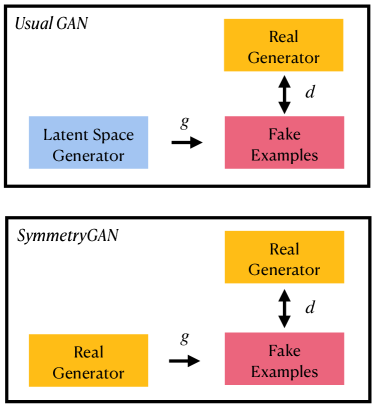
An alternative symmetry discovery approach that is flexible, fully differentiable, and simple is based on generative models Hataya et al. (2019); Antoniou et al. (2018). Usually, a generative model is a function that maps random numbers to structured data. For example, a deep generative surrogate model can be trained such that the resulting probability density matches that of a target dataset. For symmetry discovery, by contrast, the random numbers are replaced with the target dataset itself. In this way, a well-trained generator designed to confound an adversary will implement a symmetry transformation. We call this generative model framework for symmetry discovery SymmetryGAN, since it has the same basic training strategy as a generative adversarial network (GAN) Goodfellow et al. (2014), as shown in Fig. 1.
In this paper, we extend the SymmetryGAN approach (suggested in Ref. Lim et al. (2019), but in the language of data augmentation rather than symmetries) and introduce it to the physics community. In particular, we build a rigorous statistical framework for describing the symmetries of a dataset and construct a learning paradigm for automatically detecting generic symmetries. The key idea is that symmetries of a target dataset have to be defined with respect to an inertial reference dataset, analogous to inertial frames in classical mechanics. Our deep learning setup is simpler than existing approaches and we develop an analytic understanding of the algorithm’s performance in simple cases. This in turn allows us to understand the dynamics of the machine learning as it trains from a random initialization to an element of the symmetry group. The primary purpose of this paper is to carefully demonstrate that this method of symmetry discovery works. Having done so, in the last section we move forward to a discussion of methods to infer which formal groups of symmetries are present in the dataset, a related but distinct problem which is a rich area for future research.
This rest of this paper is organized as follows. In Sec. II, we build a rigorous statistical framework for discovering the symmetries of a dataset, contrasting it with discovering the symmetries of an individual data element. Our machine learning approach with an inertial restriction is introduced in Sec. III and the deep learning implementation is described in Sec. IV. Empirical studies of simple Gaussian examples, including both analytic and numerical results, are presented in Sec. V. We then apply our method to a high energy physics dataset in Sec. VI. In Sec. VII, we discuss possible ways to go beyond symmetry discovery and towards symmetry inference, with further studies in App. A. Our conclusions and outlook are in Sec. VIII.
II Statistics of Symmetries
What is a symmetry? Let be a random variable on an open set , and let be an instantiation of . When we refer to the symmetry of an individual data element , we usually mean a transformation such that:
| (1) |
i.e. is invariant to the transformation . More generally, we can consider functions of individual data elements, . In that case, the function is symmetric if
| (2) |
i.e. the output of is invariant to the transformation acting on . One can also consider equivariances, where the output of has well-defined transformation properties under the symmetry Dolan and Ore (2020); Serviansky et al. (2020); Bogatskiy et al. (2020); Shimmin (2021). While symmetries acting on individual data elements are interesting, they are not the focus of this paper.
We are interested in the symmetries of a dataset as a whole, treated as a statistical distribution. Let be governed by the probability density function (PDF) . Naively, a symmetry of the dataset is a map such that preserves the PDF:
| (3) |
where is the Jacobian determinant of . While it is necessary that any candidate symmetry preserves the probability density, it is not sufficient, at least not in the usual way that we, as particle physicists, think about symmetries.
Consider the simple case of . Let be the cumulative distribution function (CDF) of . is itself a random variable satisfying
| (4) |
where is the uniform random variable on . Conversely, is a random variable governed by the PDF (for technical details, see Ref. Angus (1994)). The uniform distribution on the interval has many PDF-preserving maps, such as the quantile inversion map:
| (5) |
This map has the additional property that , so it appears to represent a (i.e. parity) symmetry. Using the CDF map from above, every probability density admits a PDF-preserving map:
| (6) |
where refers to functional composition.
If we were to accept Eq. (3) as the definition of a symmetry, then all one-dimensional random variables would have a symmetry, namely the one in Eq. (6). While true in a technical sense, this is not what particle physicists (or, to our knowledge, any domain experts) think of as a symmetry of a dataset. The precise definition of a symmetry must therefore be stricter than simply PDF-preserving. In particular, while this PDF-preserving map applies to every one-dimensional random variable, it requires a different map for each such variable. When we usually think about symmetries, we imagine common maps that can be applied to a variety of physical systems that share the same underlying symmetry structure.
This line of thinking suggests a sharper definition of a symmetry that makes use of a reference distribution. Consider two probability density functions
| (7) |
where is the set of non-negative real numbers. A map is defined to be a symmetry of relative to if it is PDF-preserving for both and :
| (8) |
The reference or inertial density is the analogue of an inertial reference frame in classical mechanics. This new definition of a symmetry will typically exclude quantile maps, like above, because the that works for one random variable will typically not work for another (e.g. Gaussian and exponential random variables).
While this new definition solves the problem of “fake” symmetries, it also introduces a dependence on the inertial distribution. Just as with inertial reference frames, however, there is often a canonical choice for which reduces the number of possibilities in practice. A natural choice for many physics datasets is to pick the uniform distribution on , where is the dimension of the dataset, because many physics problems outside of General Relativity are set either in Euclidian space or in Lorentzian space , and the affine groups discussed above are independent of signature . This not a proper (i.e. normalizable) probability density because is a non-compact space,111A compact space is a topological space that is closed and bounded. so we discuss techniques below to use it as the inertial distribution nonetheless.
Finally, it is instructive to relate the definitions of symmetries for datasets and functions. Given the two PDFs in Eq. (7), we can construct the likelihood ratio
| (9) |
Applying the symmetry map as in Eq. (8), the likelihood ratio transforms as:
| (10) |
where the Jacobian factor cancels between the numerator and denominator. Therefore the likelihood ratio, which is an ordinary function, is symmetric by the definition in Eq. (2). This cancelling of the Jacobian factor is an intuitive way to understand why an inertial reference density is necessary to define the symmetry of a dataset.
III Machine Learning with Inertial Restrictions
The SymmetryGAN paradigm for discovering symmetries in a dataset involves simultaneously learning two functions:
| (11) | ||||
| (12) |
The function is a generator that represents the symmetry map.222Here, we are using the machine learning meaning of a “generator”, which differs from the generator of a symmetry group, though they are closely related. The function is a discriminator that tries to distinguish the input data from the transformed data . When the discriminator cannot distinguish the original data from the transformed data, then will be a symmetry. The technical details of this approach are provided in Sec. IV using the framework of adversarial networks. The generator is randomly initialized on the search manifold, and through gradient descent, converges to the nearest symmetry. It is possible that the nearest symmetry is the identity transformation, in which case the generator will converge to the identity map. When the generator is randomly initialized across the search manifold several times, however, there is no reason why the nearest symmetry on that manifold should always be the identity map, so the generator will converge to the nearest non-trivial symmetry. In fact, when the dataset respects a continuous symmetry group, the probability of the generator converging to the identity is zero.
As described in Sec. II, it is not sufficient to require that preserves the PDF of the input data; it also has to preserve the PDF of the inertial density. There are several methods to implement an inertial restriction into the machine learning strategy.
-
•
Simultaneous discrimination: In this method, the discriminator is applied both to the input dataset and to data drawn from the inertial density . The training procedure penalizes any map that does not fool for both datasets. In practice, it might be advantageous to use two separate discriminators and for this approach.
-
•
Two stage selection: Here, one first identifies all PDF-preserving maps . Then one post hoc selects the ones that also preserve the inertial density.
-
•
Upfront restriction: If the PDF-preserving maps of are already known, then one could restrict the set of maps at the outset. This allows one to perform an unconstrained optimization on the restricted search space.
Each of these methods has advantages and disadvantages. The first two options require sampling from the inertial density . This is advantageous in cases where the symmetries of the inertial density are not known analytically. When is uniform on or another unbounded domain, though, these approaches are not feasible.333One could try to leverage approximate strategies, such as cutting off the support for a few standard deviations away from the mean of . Still, one can run into edge effects if there is a mismatch between the domain and range of . The second option is computationally wasteful, as the space of PDF-preserving maps is generally much larger than the space of symmetry maps. We focus on the third option: restricting the set of functions to be automatically PDF-preserving for . This in turn requires a way to parametrize all such , or at least a large subset of them.
For all of the studies in this paper, we further focus on the case where the inertial distribution is uniform on . For any open set , a differentiable function preserves the PDF of the uniform distribution if and only if is an equiareal map.444By carefully taking suitable limits, these ideas go through even if is an improper prior. The important takeaway is that uniform distributions are preserved by equiareal maps. To see this, note that the PDF of is , where is the volume. Hence, the PDF-preserving condition is met if and only if . A map is equiareal if and only if its Jacobian determinant is , which proves our claim. Therefore, our search space to discover symmetries of physics datasets will be the space of equiareal maps of appropriate dimension. Of course, there are interesting physics symmetries that do not preserve uniform distributions on ; these would require an alternative approach.
The set of equiareal maps for is not well characterized. For example, even for , not all equiareal maps are linear. A simple example of a non-linear area-preserving map is the Hénon map Hénon (1969): . This makes the space of equiareal maps difficult to directly encode into the learning. While the general set of equiareal maps is difficult to parametrize, the set of area preserving linear maps on is well understood:
This is a subgroup of the general affine group , and it can be characterized as a topological group555A topological group is a topological space with a group operation defined on it, and where the group operation and inversion are continuous functions. of dimension . These maps even have complete parametrizations such as the Iwasawa decomposition Iwasawa (1949) which significantly aid the symmetry discovery process.
Not all symmetries are linear, however, and if one chooses as the search space, one cannot discover non-linear maps. Even so, the subset of symmetries discoverable within is rich enough, and the benefits of having a known parametrization valuable enough, that we focus on linear symmetries in this paper and leave the study of non-linear symmetries to future work.
IV Deep Learning Implementation
To implement the SymmetryGAN procedure, we modify the learning setup of a GAN Goodfellow et al. (2014). For a typical GAN, a generator function surjects a latent space onto a data space.666While all the GANs discussed here are (approximately) bijective, GANs in general need not be. Symmetry discovery requires the generator to be bijective, so one may want to leverage nomalizing flows Rezende and Mohamed (2015); Kobyzev et al. (2020) in future work. Then, a discriminator distinguishes generated examples from target examples.
For a SymmetryGAN, the latent probability density is the same as the target probability density, as illustrated in Fig. 1. The generator and discriminator are parametrized as neural networks. Following Sec. III, we construct the generator such that it is guaranteed to preserve the inertial distribution, e.g. it is an area-preserving linear transformation, but the discriminator has no such restriction. These two neural networks are then trained simultaneously to optimize the binary cross entropy loss functional, where the generator tries to maximize the loss with respect to and the discriminator tries to minimize the loss with respect to . The binary cross entropy loss functional is:
| (13) |
This differs from the usual binary cross entropy in that the same samples appear in the first and second terms. A similar structure appears in neural resampling Nachman and Thaler (2020) and in step 2 of the OmniFold algorithm Andreassen et al. (2020).
We now show that optimizing the above loss corresponds to finding a symmetry generator . The behavior of Eq. (13) can be understood analytically by considering the limit of infinite data:
| (14) |
where the Jacobian factor is now made manifest. For a fixed , the optimal is the usual result from binary classification (see e.g. Ref. Hastie et al. (2001); Sugiyama et al. (2012)):
| (15) |
which is the ratio of the probability density of the first term in Eq. (14) to the sum of the densities of both terms. We then insert into Eq. (14) and optimize using the Euler-Lagrange equation:
| (16) |
By use of a computer algebra system capable of solving simple differential equations (in our case, Mathematica Inc. ), one can show that the optimal satisfies
| (17) |
i.e. is PDF preserving as in Eq. (3). For such a , we have that , the loss is maximized at a value of , and the discriminator is maximally confounded.
The SymmetryGAN approach has the potential to find any symmetry representable by . To target a particular symmetry subgroup, , we can add a term to the loss function. For example, to discover a cyclic symmetry group, , the loss function can be augmented with a mean squared error term:
| (18) |
where is the binary cross entropy loss in Eq. (13), is composed with itself times, and is a weighting hyperparameter. A SymmetryGAN with this loss function will discover the largest subgroup of that is a symmetry of the dataset.
V Empirical Gaussian Experiments
In this section, we study the SymmetryGAN approach both analytically and numerically in a variety of simple Gaussian examples. For the empirical studies here and in Sec. VI, all neural networks are implemented using the Keras Chollet (2017) high-level API with the Tensorflow2 backend Abadi et al. (2016) and optimized with Adam Kingma and Ba (2014). The generator function is parametrized as a linear function, with constraints that vary by example and are described further below. The discriminator function is parametrized with two hidden layers, using 25 nodes per layer. Rectified Linear Unit (ReLU) activation functions are used for the intermediate layers and a sigmoid function is used for the last layer. For the empirical studies, events are generated for each example.
V.1 One-Dimensional Gaussian
Our first example involves data drawn from a one-dimensional Gaussian distribution with a reflection symmetry. Data are distributed according to the probability distribution i.e. a Gaussian with and . This distribution has precisely two symmetries, both linear:
| (19) |
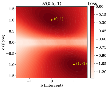
Implicitly, we are taking the inertial distribution to be uniform on . As stated earlier, the PDF-preserving maps of are equireal. In one dimension, the only equireal maps are linear. Linear maps in one dimension are defined by two numbers, so the generator function can be parametrized as
| (20) |
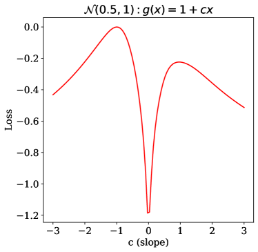
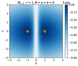
In Fig. 2, we show the analytically computed loss from Eq. (14) as a function of and . In this figure, the discriminator is taken to be the analytic optimum in Eq. (15). There are two maxima in the loss landscape, one corresponding to each of the linear symmetries from Eq. (19). Here, and in most subsequent examples below, we have shifted the output such that maximum loss value is .
Another interesting feature of the loss landscape is the deep minimum at that divides the space into two parts. This gives rise to the prediction that, under gradient descent, the neural network will find when is initialized negative and find when is initialized positive. In the edge case when is initialized to precisely zero, the generator is degenerate and no longer even bijective and the outcome is indeterminate, but the likelihood of sampling to be precisely zero is, of course, zero. For the rest of the paper, we ignore such edge cases. There are no such features in the loss landscape as a function of , suggesting that there should be little dependence on the initial value of .
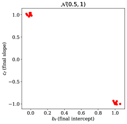
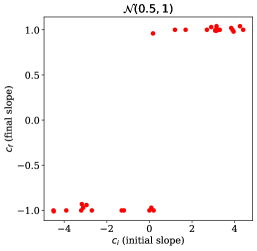
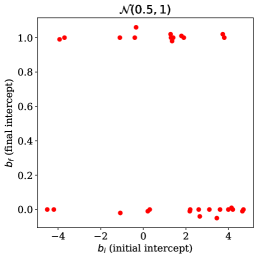
These predictions are tested empirically in Fig. 3, where the initialized parameters are and the learned parameters are . In Fig. 3i, there are distinct clusters at and , showing that the SymmetryGAN correctly finds both symmetries of the distribution and nothing else. In Fig. 3ii, there is a demonstration of the loss barrier in slope space; if the initial slope is positive, the final slope is , whereas if the initial slope is negative, the final slope is . Finally, Fig. 3iii shows the absence of a loss barrier in intercept space; the final intercepts are scattered between and independent of the initialized intercept. We discuss further the symmetry discovery map from initialized to learned parameters in Sec. VII.3 and App. A.
In the above example, the parametrization of was sufficiently flexible that the SymmetryGAN could find both symmetries and the loss landscape had no other maxima. If the space is incompletely parametrized, though, then local maxima can manifest as false symmetries. For example, suppose instead of a two parameter as above, were parameterized as . The corresponding analytic loss landscape is shown in Fig. 4. A SymmetryGAN initialized with a negative slope correctly finds the only symmetry of this form, , but a neural network initialized with positive slope is unable to cross over the loss barrier at and instead settles at the locally loss maximizing . While our investigations of suggest that this does not happen with the full parametrization, the topology of the set of equiareal maps is not known and therefore obstructions like the one illustrated here are possible. It is always possible to check if a solution is a symmetry, however. Specifically, one can apply the learned function to the data and train a post hoc discriminator to ensure that its performance is equivalent to random guessing. For an analytic symmetry, we know that at the point of loss maximization , and consequently . Hence, at the global (symmetry) maxima, . On the other hand, there is no way for the neural network to get stuck at non-symmetry local maxima with . Hence, the true symmetries can be distinguished from local optima by checking the value of the loss.
V.2 Two-Dimensional Gaussian
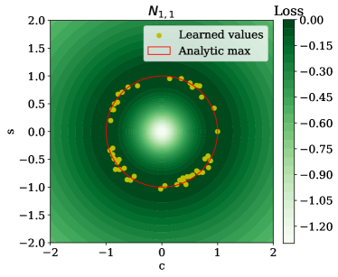
Next, we consider cases of two-dimensional Gaussian random variables. These examples offer much richer symmetry groups for study as well as a greater scope for variations. We take the inertial distribution to be uniform on .
We start with the standard normal distribution in two dimensions,
| (21) |
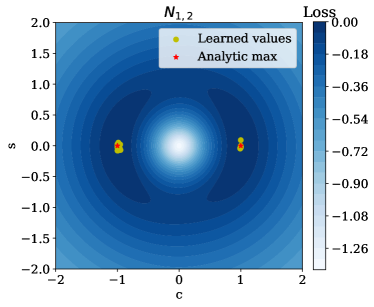
where is the identity matrix. This distribution has as its linear symmetries all rotations about the origin and all reflections about lines through the origin, which constitute the group . For further exploration, we consider a two-dimensional Gaussian with covariance not proportional to the identity,
| (22) |
The symmetry group of this distribution is quite complicated and described below. Among other features, it contains the Klein 4–group, , for Pauli matrix .
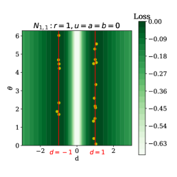
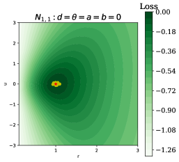
The linear search space that preserves , the general affine group in two dimensions, , has six real parameters. Before exploring the entire space, we first examine the subspace:
for , where is the set of non-zero real numbers. While this is only a rotation if , we want to test if a SymmetryGAN can discover this relationship starting from this more general representation. The symmetries represented by Eq. (V.2) are a subgroup of : , where is the set of positive real numbers. For the Gaussian, this means looking for the subgroup, which is indicated by the red circle in the loss landscape in Fig. 5i. To test the SymmetryGAN, we sample the parameters and uniformly at random from , and the learned and values correspond to the expected unit circle, also shown in Fig. 5i. We repeat this exercise for the Gaussian in Fig. 5ii, where the SymmetryGAN discovers the subgroup of generated by a rotation by .
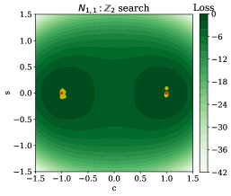
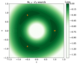
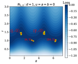
This two-dimensional example allows us to test the approach in Eq. (18) for finding subgroups of the full symmetry group. Restricting our attention to the example and the subgroup in Eq. (V.2), we add the cyclic-enforcing mean squared error term to the loss with . Results are shown in Fig. V.2 for , , and , where the analytic loss optima and empirically found symmetries are broken into discretely many solutions, with the number corresponding to the roots of unity, as expected.
We now consider the general affine group, . In two dimensions, the elements of this group can be represented as a matrix with 6 parameters:
-
•
, the determinant;
-
•
, the angle of rotation;
-
•
, the dilatation;
-
•
, the shear in the direction; and
-
•
the overall affine shift.
By Iwasawa’s decomposition Iwasawa (1949), the full transformation can be written as
V.3 Gaussian Mixtures
As our last set of simple examples, we apply the SymmetryGAN approach to three Gaussian mixture models, inspired by the examples in Ref. Fisher et al. (2018). The first is a one-dimensional bimodal probability distribution:
| (23) |
which respects the symmetry group . The empirical distribution for this example is shown in Fig. LABEL:fig:otherdistributions_1Di. Applying SymmetryGAN starting from the generator for linear transformations in Eq. (20), it finds the predicted symmetries with great accuracy, as shown in Fig. LABEL:fig:otherdistributions_1Dii.
We next consider two two-dimensional Gaussian mixtures. The octagonal distribution,
| (24) |
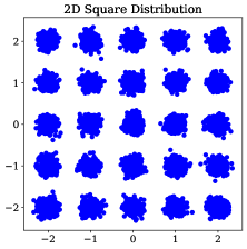
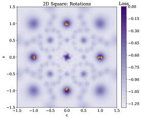
has the dihedral symmetry group of an octagon . The two-dimensional square distribution,
| (25) |
has the symmetry group of a square . We use the generator
| (26) |
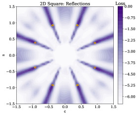
which can discover the the entire symmetry subgroup (rotations and reflections) in . Data sampled from these distributions are shown in the left column of Fig. 8i. In the middle and right columns of Fig. 8i, we see that SymmetryGAN finds the expected rotations and reflections, respectively.
VI Particle Physics Example
We now turn to an application of SymmetryGANs in particle physics. Here, we are interested to learn if this approach can recover well-known azimuthal symmetries in collider physics and possibly identify symmetries that are not immediately obvious. By the Coleman–Mandula theorem Coleman and Mandula (1967), space-time and internal symmetries cannot be combined in any but a trivial way. Ergo, from momentum data, the only symmetry groups that can be discovered are subgroups of the Poincaré group, . There is much to be explored and studied within the Poincaré group itself, however. We do not even have a complete classification of its unitary representations Ohnuki et al. (1988); Wigner (1939) and its subgroup structure is remarkably rich and complex. Discovering which specific subgroup of the Poincaré group constitutes the symmetry group of the system at hand is a non-trivial question, one we can seek to address through SymmetryGAN.
VI.1 Dataset and Preprocessing
This case study is based on dijet events. Jets are collimated sprays of particles produced from the fragmentation of quarks and gluons, and pairs of jets are one of the most common configurations encountered at the LHC. With a suitable jet clustering algorithm, each jet has a well-defined momentum, and we can search for symmetries of the jet momentum distributions.
The dataset we use is the background dijet sample from the LHC Olympics anomaly detection challenge Kasieczka et al. (2019, 2021). These events are generated using Pythia 8.219 Sjöstrand et al. (2006, 2008) with detector simulation provided by Delphes 3.4.1 de Favereau et al. (2014); Mertens (2015); Selvaggi (2014) The reconstructed particle-like objects in each event are clustered into anti- Cacciari et al. (2008) jets using FastJet 3.3.0 Cacciari et al. (2012); Cacciari and Salam (2006). All events are required to satisfy a single TeV jet trigger, and our analysis is based on the leading two jets in each event, where leading refers to the ones with largest transverse momenta ().
Each event is represented as a four-dimensional vector:
| (27) |
where refers to the momentum of the leading jet, represents the momentum of the subleading jet, and and are the Cartesian coordinates in the transverse plane. We focus on the transverse plane because the jets are typically back-to-back in this plane as a result of momentum conservation. The longitudinal momentum of the parton-parton interaction is not known and so there is no corresponding conservation law for .777In principle, we could use SymmetryGAN to confirm the absence of a symmetry in .
Since we have a four-dimensional input space, a natural search space for symmetries is , the group of all rotations on . Before exploring the whole candidate symmetry space, we first consider an subspace where the two leading jets are independently rotated.
VI.2 Subspace
Because of momentum conservation, we expect that only those rotations that simultaneously rotate both jets by the same angle will be symmetries. We start from a generic group element:
| (28) |
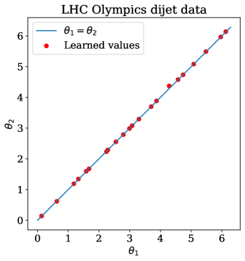
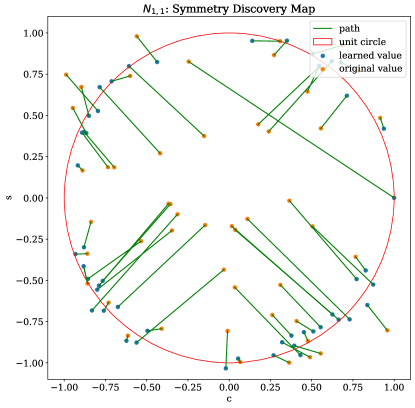
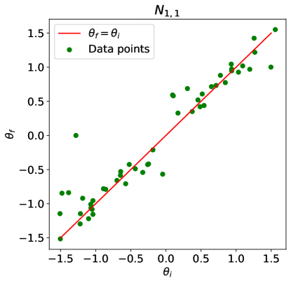
where . We expect the symmetries to correspond to the subgroup . This prediction is borne out in Fig. 11i.
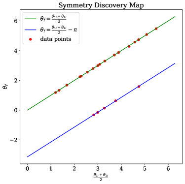
We can also study the training dynamics of the SymmetryGAN. More information about this procedure is given in App. A, but the idea is to find a symmetry discovery map , that describes how the initial parameters map to the learned ones. We propose the map given by
| (29) |
where there is only one output angle even though the output space is two-dimensional. This map posits that the final angle will bisect the smaller angle between and , which is validated by the empirical results shown in Fig. 11ii.
VI.3 Search Space
We now turn to the four-dimensional rotation group. is a six parameter group, specified by which parametrize the six independent rotations:
| (30) | ||||||
| (31) | ||||||
| (32) |
where the notation means
| (33) | ||||
| (34) |
One way to describe a generic generator is by
| (35) |
It is not easy to visualize a six-dimensional space, and the symmetries discovered by SymmetryGAN do not lie in any single -plane or even -plane. Therefore, we need alternative methods to verify that the maps discovered by the neural network are indeed symmetries.
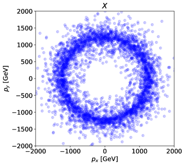
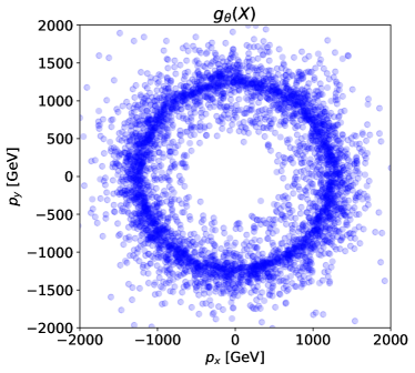
One verification strategy is to visually inspect and to see if the spectra look the same. In Fig. 12, we show a projection of the distribution of and one instance of , which suggests that the found is indeed a symmetry.
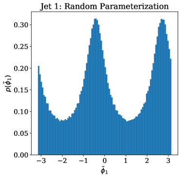
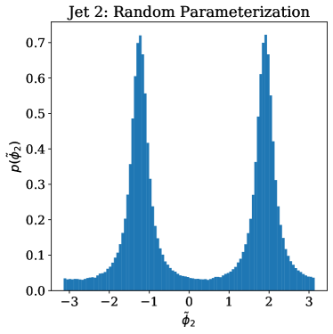
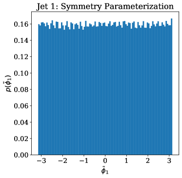
Another verification strategy is to test if the discovered symmetries preserve special projections of the dataset. Each of the two jets has an azimuthal angle for that is uniformly distributed over , where arctan2 is the two argument arctangent function, which returns the principal value of the polar angle . Symbolically, the data can be represented as
| (36) |
where is the transverse momentum of each jet (which is approximately the same for both jets since they are roughly back to back). If one applies an arbitrary rotation, there is no reason the new azimuthal angles,
| (37) | ||||
| (38) |
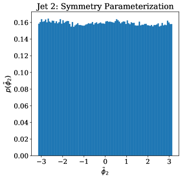
should be uniformly distributed anymore, as Fig. 13 demonstrates. If one of the symmetry rotations discovered by the neural network is applied to , however, must remain uniformly distributed, as shown in Fig. 14.
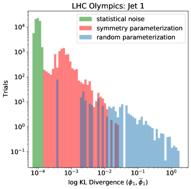
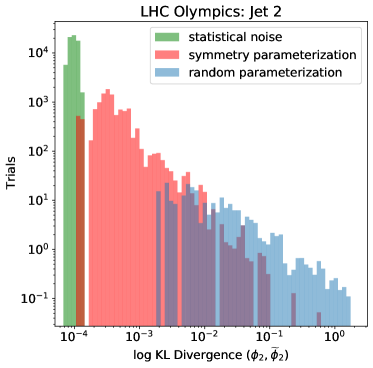
This effect can be quantified by computing the Kullback-Leibler (KL) divergence of the two distributions against that of . In Fig. 15, we see that the KL divergence of the symmetries is much smaller than the KL divergence of the random rotations. Also plotted on the same figure is the KL divergence of two samples drawn from , which represents the irreducible effect from considering a finite dataset. This would be the KL divergence of obtained from applying an ideal analytic symmetry to , against . It is instructive to consider the means of the histograms. The KL divergence of randomly selected elements of has means of () for the leading (subleading) jet, while the KL divergence of symmetries in has respective means (). The irreducible statistical noise has a mean of .
Clearly, the symmetries reconstruct the distribution much better than randomly selected elements of , and are in fact quite close to the irreducible KL divergence due to finite sample size. Note that the x-axis of Fig. 15 is logarithmic, which magnifies the region near zero, so the difference between the symmetry histogram and the statistical noise histogram is smaller than it might appear.
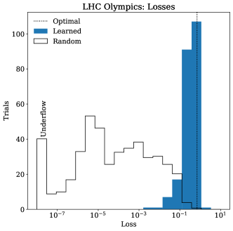
A final method to independently verify that the rotations SymmetryGAN finds are symmetries of the LHC Olympics data is by computing the loss function. As discussed at the end Sec. V.1, when represents a symmetry and is an ideal discriminator, the binary cross entropy loss is . By training a post hoc classifier, we can therefore compute the loss of a specific symmetry generator.888In principle, one could look at the value of the loss after training the discriminator. In practice, a post-hoc classifier yields more reliable behavior; see related discussion in Ref. Diefenbacher et al. (2020). In Fig. 16, we compare the loss of randomly sampled rotations from to the loss of rotations discovered by SymmetryGAN. The latter is quite close to the analytic optimum, .
From these tests, we conclude that SymmetryGAN has discovered symmetries of the LHC Olympics dataset. As discussed further in Sec. VII below, though, discovering symmetries is different from inferring the structure of the found subgroup from the six-dimensional search space. Mimicking the study from Fig. 6i, we can study its subgroups, through the loss function in Eq. (18) with . The backbone of this subgroup is expected to be the reflections (because both jets have approximately the same momenta) and (because and look the same upon drawing sufficiently many samples of ). The learning process reveals a much larger group, though. There is in fact a continuous group of symmetries, which combine an overall azimuthal rotation and one of the aforementioned backbone reflections. In retrospect, these symmetries should have been expected, since they are compositions of well-known symmetry transformations. This example highlights the need to go beyond symmetry discovery and towards symmetry inference.
VII Towards Symmetry Inference
The examples in Secs. V and VI highlight the potential power of SymmetryGAN for discovering symmetries using deep learning. Despite the many maps discovered by the neural network, though, it is difficult to infer, for example, the precise Lie subgroup of respected by the LHC Olympics data. This highlights a limitation of this approach and the distinction between “symmetry discovery” and “symmetry inference”. Though SymmetryGAN can identify points on the Lie group manifold, there is no simple way to infer precisely which Lie group has been discovered. While symmetry discovery is sufficient for the data augmentation described in previous sections to facilitate data analysis, it is of theoretical interest to infer which formal Lie groups comprise the symmetries of our collider data. In this section, we mention three potential methods to assist in the process of symmetry inference.
VII.1 Finding Discrete Subgroups
One way to better understand the structure of the learned symmetries is to look for discrete subgroups. As already shown in Fig. V.2 and mentioned in the particle physics case, we can identify discrete symmetry transformations by augmenting the loss with Eq. (18). By forcing the symmetries to take a particular form, we can infer the presence (or absence) of such a subgroup.
It is interesting to consider possible modifications to Eq. (18) to handle non-Abelian discrete symmetries. The goal would be to learn multiple symmetries simultaneously that satisfy known group theoretic relations. For example in the Abelian case, a loss term like
| (39) |
could be used to identify any two symmetries and that commute. We leave a study of these possibilities to future work.
VII.2 Group Composition
By running SymmetryGAN a few times, one may discover a few points on the symmetry manifold. By composing these discovered symmetries together, one can rapidly increase the number of known points on the manifold because the discovered symmetries are elements of a group, by construction, so their composition is still an element of the group.
This notion is quite powerful. The ergodicity of the orbits of group elements is a richly studied and complex area of mathematics (see e.g. Ref. Zimmer (1982)). Many groups of physical interest are locally connected, compact, and have additional structure. In that context, it is likely that the full symmetry group is generated by , where is randomly drawn from the group and is the product of the representation dimension and the number of connected components.
For example, consider the group , which has . Almost any element of , has rotation angle which is an irrational multiple of . We can therefore approximate any element by repeated applications of :
| (40) |
In other words, the subgroup generated by is dense in .
In practice, the symmetries discovered by SymmetryGAN will be not exact due to numerical considerations. Since the network learns approximate symmetries with some associated error, each composition compounds this error. Thus, there are practical limits on the number of compositions that can be carried out with numeric data.
VII.3 The Symmetry Discovery Map
So far, we have initialized a SymmetryGAN with uniformly distributed values of certain parameters, and then trained it to return the values of those parameters that constitute a symmetry. We can define a symmetry discovery map, which connects the initialized parameters of to the parameters of the learned function:
| (41) |
where is the dimension of the parameter space. This is a powerful object not only for characterizing the learning dynamics but also to assist in the process of symmetry discovery and inference.
There are at least two distinct reasons why knowledge of this symmetry discovery map is useful. First, the map is of theoretical interest. We discussed in Sec. V.1 the importance of understanding the topology of the symmetry group. The symmetry discovery map induces a deformation retract from the search space to the symmetry space. Every deformation retract is a homotopy equivalence, and by the Eilenberg-Steenrod axiom of homotopy equivalence Eilenberg and Steenrod (1945), the homology groups of the symmetry group can be constructed from the homology groups of the search space. Even in low dimensions, the topology of the symmetry group can be non-trivial (cf. Sec. V.2 for an example in 2D). The topology of , however, has been studied for over half a century, and the homotopy and homology groups of several non-trivial subgroups of have been fully determined Schlichting (2017). Hence, if the symmetry discovery map were known, one could leverage the full scope of algebraic topology and the known results for the linear groups to understand the topology of the symmetry group.
Second, this map has practical value. Every time a SymmetryGAN is trained, it must relearn how to move the initialized values of to the final values. Intuitively, nearby initial values should map to nearby final values, so learning the symmetry discovery map should enable a more efficient exploration of the symmetry group. In practice, this can be accomplished by augmenting the loss function in Eq. (13). Let be the symmetry generator, with the parameters made explicit. Let be a neural network representing the symmetry discovery map. Sampling parameters from the space of parameters and data points from , we can optimize the following loss:
| (42) | ||||
Note that this loss is now a functional of instead of . If can be initialized to the identity function, then gradient descent acting on is (asymptotically) the same as gradient descent acting on the original parameters. Thus, as long as has a sufficiently flexible parametrization, the learned will be a good approximation to the symmetry discovery map learned by the original SymmetryGAN.
We defer a full exploration of the symmetry discovery map to future work. Preliminary analytic and numerical studies of the symmetry discovery map are shown in App. A.
VIII Conclusions and Outlook
In this paper, we provided a rigorous statistical definition of the term “symmetry” in the context of probability densities. This is highly relevant for the field of high energy collider physics where the key objects of study are scattering cross sections. We proposed SymmetryGAN as a novel, flexible, and fully differentiable deep learning approach to symmetry discovery. SymmetryGAN showed promising results when applied to Gaussian datasets as well as to dijet events from the LHC, conforming with our analytic predictions and providing new insights in some cases.
A key takeaway lesson is that the symmetry of a probability density only makes sense when compared to an inertial density. For our studies, we focused exclusively on the inertial density corresponding to the uniform distribution on (an open subset of) , since Euclidean symmetries are ubiquitous in physics. Furthermore, we only considered area preserving linear maps on , a simple yet rich group of symmetries that maintain this inertial density. This method has great utility for data analysis. The symmetries of a dataset discovered by SymmetryGAN can be used to augment a dataset, thereby increasing its statistical power substantially. Conversely, it could be used to preprocess the data to explicitly project out symmetries and fix a preferred reference frame, thereby once again boosting the data analysis process substantially. Moving forward, there are many opportunities to further develop the concepts introduced in this paper. As a straightforward extension, non-linear equiareal maps over could be added to the linear parametrizations we explored, as could Lorentz-like symmetries. In more complex cases where there is no obvious notion of an inertial density, one could study the relative symmetries between two different datasets. It would also be interesting to discover approximate symmetries and rigorously quantify the degree of symmetry breaking. This is relevant in cases where the complete symmetry group is obscured by experimental acceptances and efficiencies.
A key open question is how to go beyond symmetry discovery and towards symmetry inference. We showed how one can introduce loss function modifications to emphasize the discovery of discrete subgroups. One could imagine extending this strategy to continuous subgroups to gain a better handle on group theoretic structures. The symmetry discovery map is a potentially powerful tool for symmetry inference, since it in principle allows the entire symmetry group to be discovered in a single training. In practice, though, we found learning the symmetry discovery map to be particularly challenging. We hope future algorithmic and implementation developments will enable more effective strategies for symmetry discovery and inference, in particle physics and beyond.
The code for this paper can be found in this GitHub repository.
Acknowledgments
We would like to thank Andrew Larkoski for his thoughtful comments and feedback. KD and BN are supported by the U.S. Department of Energy, Office of Science under contract DE-AC02-05CH11231. JT is supported by the National Science Foundation under Cooperative Agreement PHY-2019786 (The NSF AI Institute for Artificial Intelligence and Fundamental Interactions, http://iaifi.org/), and by the U.S. DOE Office of High Energy Physics under grant number DE-SC0012567.
Appendix A Explorations of the Symmetry Discovery Map
In this appendix, we initiate a study of the symmetry discovery map from Sec. VII.3, both analytically and numerically.
A.1 One-Dimensional Gaussian
In the simplest cases, the symmetry discovery map can be determined analytically, and a neural network can be used to independently verify that the proposed map is indeed the symmetry discovery map. For example, consider the one-dimensional Gaussian example from Sec. V.1, where the probability distribution is and the candidate symmetry transformations take the form for . There are two symmetries in this case: the identity and .
In Sec. V.1, we conjectured that the learned symmetry is the one on the same side of the loss barrier at as the initialization. This means that independent of , if , then will be the identity and if , will be the inversion map. Symbolically, the symmetry discovery map takes the form
| (43) |
The numerical results already shown in Fig. 3 verify that is indeed the correct symmetry discovery map.
A.2 Two-Dimensional Gaussian
We next consider one of the two-dimensional Gaussian examples from Sec. V.2. The probability distribution is and the candidate symmetry transformations are
| (44) |
From analyzing the loss landscape, we expect the neural network to map the initialized point to the nearest point on along a radius of the unit circle. This leads to the symmetry discovery map:
| (45) |
In Fig. 17i, we show the numerical mapping between initial and final parameters, corresponding to the plot in Fig. 5i. The radial behavior is clearly visible, although there are some outliers that could be due to incomplete training and the stochastic nature of the gradient decent.
We can gain more insight by studying this behavior in polar coordinates:
| (46) |
Going back to and can be done with the inverse mapping and . In polar coordinates, the symmetry discovery map is rather simple:
| (47) |
The numerics support this prediction, as shown in Fig. 17ii. The initialized and learned points collect around the line of constant polar angle.
A.3 Learning the Symmetry Discovery Map
Ultimately, the symmetry discovery map will be most useful if it can be learned from a single training run. In preliminary studies, however, we encountered two key challenges.
The first challenge is that, for to approximate the symmetry discovery map, it needs to be initialized to the identity function. If the goal is just to find a family of symmetries, then it would be fine to start from a randomly initialized neural network. In that case, would be a parametrized symmetry network, in the spirit of Ref. Baldi et al. (2016). But for the goal of finding the symmetry discovery map, one needs a parametrization of that is flexible enough to describe the map, but simple enough that it can be initialized close to the identity.
The second challenge is that performing min-max optimization of Eq. (42) seems particularly finicky. GANs are known to exhibit issues like mode collapse, and because the target space of the symmetry discovery map is often disjoint, these kinds of issues seem to arise in our case as well.
Consider the simple case of learning the symmetry discovery map for data and the generator . We know that the symmetries of are . Therefore, the symmetry discovery map should be the step function :
| (48) |
The form in Eq. (48) is not so easy to learn with any of the standard neural network activation functions, though. The one exception is unit step activation, of course, but this activation is far from the identity and therefore difficult to use for finding a symmetry discovery map.
One approach to this problem is to use a custom activation function:
| (49) |
This can be initialized at , so that in the beginning . As moves away from , this function develops a non-linearity as desired. With a single layer, this form is not sufficient to learn the correct answer, though it may be possible that with a deep network stacked with these components, the correct map could be learned.
Another approach to this problem is to use polynomial activation,
| (50) |
initialized with . A step function is not within this class of functions, but with such a high degree polynomial, it is expected to be a reasonable approximation. This was in fact the case, though the result was far from satisfactory.
Finally, as a proof of principle, we tested the simplified ansatz:
| (51) |
When initialized with the identity function (), gradient descent indeed converges to Eq. (48) (). This ansatz is too contrived to draw any robust conclusions, but is does motivate future exploration of more complex architectures and training protocols to learn the symmetry discovery map.
References
- LeCun et al. (1989) Y. LeCun, B. Boser, J. S. Denker, D. Henderson, R. E. Howard, W. Hubbard, and L. D. Jackel, “Backpropagation applied to handwritten zip code recognition,” Neural Computation 1, 541–551 (1989).
- Butter et al. (2020) A. Butter, S. Diefenbacher, G. Kasieczka, B. Nachman, and T. Plehn, “GANplifying Event Samples,” (2020), arXiv:2008.06545 [hep-ph] .
- Dillon et al. (2021) Barry M. Dillon, Gregor Kasieczka, Hans Olischlager, Tilman Plehn, Peter Sorrenson, and Lorenz Vogel, “Symmetries, Safety, and Self-Supervision,” (2021), arXiv:2108.04253 [hep-ph] .
- Greydanus et al. (2019) Sam Greydanus, Misko Dzamba, and Jason Yosinski, “Hamiltonian neural networks,” (2019), arXiv:1906.01563 [cs.NE] .
- Cranmer et al. (2020) Miles Cranmer, Sam Greydanus, Stephan Hoyer, Peter Battaglia, David Spergel, and Shirley Ho, “Lagrangian neural networks,” (2020), arXiv:2003.04630 [cs.LG] .
- Barenboim et al. (2021) Gabriela Barenboim, Johannes Hirn, and Veronica Sanz, “Symmetry meets AI,” (2021), arXiv:2103.06115 [cs.LG] .
- Krippendorf and Syvaeri (2020) Sven Krippendorf and Marc Syvaeri, “Detecting Symmetries with Neural Networks,” (2020), arXiv:2003.13679 [physics.comp-ph] .
- Zhou et al. (2021) Allan Zhou, Tom Knowles, and Chelsea Finn, “Meta-learning symmetries by reparameterization,” (2021), arXiv:2007.02933 [cs.LG] .
- Benton et al. (2020) Gregory Benton, Marc Finzi, Pavel Izmailov, and Andrew Gordon Wilson, “Learning invariances in neural networks,” (2020), arXiv:2010.11882 [cs.LG] .
- Tombs and Lester (2021) Rupert Tombs and Christopher G. Lester, “A method to challenge symmetries in data with self-supervised learning,” (2021), arXiv:2111.05442 [hep-ph] .
- Lester (2021) Christopher G. Lester, “Chiral Measurements,” (2021), arXiv:2111.00623 [hep-ph] .
- Lester and Tombs (2021) Christopher G. Lester and Rupert Tombs, “Stressed GANs snag desserts, a.k.a Spotting Symmetry Violation with Symmetric Functions,” (2021), arXiv:2111.00616 [hep-ph] .
- Collins et al. (2018) Jack H. Collins, Kiel Howe, and Benjamin Nachman, “Anomaly Detection for Resonant New Physics with Machine Learning,” Phys. Rev. Lett. 121, 241803 (2018), arXiv:1805.02664 [hep-ph] .
- Collins et al. (2019) Jack H. Collins, Kiel Howe, and Benjamin Nachman, “Extending the search for new resonances with machine learning,” Phys. Rev. D99, 014038 (2019), arXiv:1902.02634 [hep-ph] .
- D’Agnolo and Wulzer (2019) Raffaele Tito D’Agnolo and Andrea Wulzer, “Learning New Physics from a Machine,” Phys. Rev. D99, 015014 (2019), arXiv:1806.02350 [hep-ph] .
- Cubuk et al. (2019) Ekin D. Cubuk, Barret Zoph, Dandelion Mane, Vijay Vasudevan, and Quoc V. Le, “Autoaugment: Learning augmentation policies from data,” (2019), arXiv:1805.09501 [cs.CV] .
- Lim et al. (2019) Sungbin Lim, Ildoo Kim, Taesup Kim, Chiheon Kim, and Sungwoong Kim, “Fast autoaugment,” (2019), arXiv:1905.00397 [cs.LG] .
- Hataya et al. (2019) Ryuichiro Hataya, Jan Zdenek, Kazuki Yoshizoe, and Hideki Nakayama, “Faster autoaugment: Learning augmentation strategies using backpropagation,” (2019), arXiv:1911.06987 [cs.CV] .
- Antoniou et al. (2018) Antreas Antoniou, Amos Storkey, and Harrison Edwards, “Data augmentation generative adversarial networks,” (2018), arXiv:1711.04340 [stat.ML] .
- Goodfellow et al. (2014) Ian J. Goodfellow, Jean Pouget-Abadie, Mehdi Mirza, Bing Xu, David Warde-Farley, Sherjil Ozair, Aaron Courville, and Yoshua Bengio, “Generative Adversarial Networks,” (2014), arXiv:1406.2661 [stat.ML] .
- Dolan and Ore (2020) Matthew J. Dolan and Ayodele Ore, “Equivariant Energy Flow Networks for Jet Tagging,” (2020), arXiv:2012.00964 [hep-ph] .
- Serviansky et al. (2020) Hadar Serviansky, Nimrod Segol, Jonathan Shlomi, Kyle Cranmer, Eilam Gross, Haggai Maron, and Yaron Lipman, “Set2graph: Learning graphs from sets,” (2020), arXiv:2002.08772 [cs.LG] .
- Bogatskiy et al. (2020) Alexander Bogatskiy, Brandon Anderson, Jan T. Offermann, Marwah Roussi, David W. Miller, and Risi Kondor, “Lorentz Group Equivariant Neural Network for Particle Physics,” (2020), arXiv:2006.04780 [hep-ph] .
- Shimmin (2021) Chase Shimmin, “Particle Convolution for High Energy Physics,” (2021) arXiv:2107.02908 [hep-ph] .
- Angus (1994) John E. Angus, “The probability integral transform and related results,” SIAM Review 36, 652–654 (1994).
- Hénon (1969) M. Hénon, “Numerical study of quadratic area-preserving mappings,” Quarterly of Applied Mathematics 27, 291–312 (1969).
- Iwasawa (1949) Kenkichi Iwasawa, “On some types of topological groups,” Annals of Mathematics 50, 507–558 (1949).
- Rezende and Mohamed (2015) Danilo Jimenez Rezende and Shakir Mohamed, “Variational inference with normalizing flows,” International Conference on Machine Learning 37, 1530 (2015).
- Kobyzev et al. (2020) Ivan Kobyzev, Simon Prince, and Marcus Brubaker, “Normalizing Flows: An Introduction and Review of Current Methods,” IEEE Transactions on Pattern Analysis and Machine Intelligence , 1 (2020).
- Nachman and Thaler (2020) B. Nachman and J. Thaler, “A Neural Resampler for Monte Carlo Reweighting with Preserved Uncertainties,” 102, 076004 (2020), arXiv:2007.11586 [hep-ph] .
- Andreassen et al. (2020) Anders Andreassen, Patrick T. Komiske, Eric M. Metodiev, Benjamin Nachman, and Jesse Thaler, “OmniFold: A Method to Simultaneously Unfold All Observables,” Phys. Rev. Lett. 124, 182001 (2020), arXiv:1911.09107 [hep-ph] .
- Hastie et al. (2001) Trevor Hastie, Robert Tibshirani, and Jerome Friedman, The Elements of Statistical Learning, Springer Series in Statistics (Springer New York Inc., New York, NY, USA, 2001).
- Sugiyama et al. (2012) Masashi Sugiyama, Taiji Suzuki, and Takafumi Kanamori, Density Ratio Estimation in Machine Learning (Cambridge University Press, 2012).
- (34) Wolfram Research, Inc., “Mathematica,” .
- Chollet (2017) Fraciois Chollet, “Keras,” https://github.com/fchollet/keras (2017).
- Abadi et al. (2016) Martín Abadi, Paul Barham, Jianmin Chen, Zhifeng Chen, Andy Davis, Jeffrey Dean, Matthieu Devin, Sanjay Ghemawat, Geoffrey Irving, Michael Isard, et al., “Tensorflow: A system for large-scale machine learning.” in OSDI, Vol. 16 (2016) pp. 265–283.
- Kingma and Ba (2014) Diederik Kingma and Jimmy Ba, “Adam: A method for stochastic optimization,” (2014), arXiv:1412.6980 [cs] .
- Fisher et al. (2018) Charles K. Fisher, Aaron M. Smith, and Jonathan R. Walsh, “Boltzmann encoded adversarial machines,” (2018), arXiv:1804.08682 [stat.ML] .
- Coleman and Mandula (1967) Sidney Coleman and Jeffrey Mandula, “All possible symmetries of the matrix,” Phys. Rev. 159, 1251–1256 (1967).
- Ohnuki et al. (1988) Y Ohnuki, S Kitakado, and T Sugiyama, Unitary Representations of the Poincaré Group and Relativistic Wave Equations (WORLD SCIENTIFIC, 1988) https://www.worldscientific.com/doi/pdf/10.1142/0537 .
- Wigner (1939) E. Wigner, “On unitary representations of the inhomogeneous lorentz group,” Annals of Mathematics 40, 149–204 (1939).
- Kasieczka et al. (2019) Gregor Kasieczka, Ben Nachman, and David Shih, “R&D Dataset for LHC Olympics 2020 Anomaly Detection Challenge,” (2019).
- Kasieczka et al. (2021) Gregor Kasieczka et al., “The LHC Olympics 2020: A Community Challenge for Anomaly Detection in High Energy Physics,” (2021), arXiv:2101.08320 [hep-ph] .
- Sjöstrand et al. (2006) Torbjorn Sjöstrand, Stephen Mrenna, and Peter Z. Skands, “PYTHIA 6.4 Physics and Manual,” JHEP 05, 026 (2006), arXiv:hep-ph/0603175 [hep-ph] .
- Sjöstrand et al. (2008) Torbjorn Sjöstrand, Stephen Mrenna, and Peter Z. Skands, “A Brief Introduction to PYTHIA 8.1,” Comput. Phys. Commun. 178, 852 (2008), arXiv:0710.3820 [hep-ph] .
- de Favereau et al. (2014) J. de Favereau, C. Delaere, P. Demin, A. Giammanco, V. Lemaitre, A. Mertens, and M. Selvaggi (DELPHES 3), “DELPHES 3, A modular framework for fast simulation of a generic collider experiment,” JHEP 02, 057 (2014), arXiv:1307.6346 [hep-ex] .
- Mertens (2015) Alexandre Mertens, “New features in Delphes 3,” Proceedings, 16th International workshop on Advanced Computing and Analysis Techniques in physics (ACAT 14): Prague, Czech Republic, September 1-5, 2014, J. Phys. Conf. Ser. 608, 012045 (2015).
- Selvaggi (2014) Michele Selvaggi, “DELPHES 3: A modular framework for fast-simulation of generic collider experiments,” Proceedings, 15th International Workshop on Advanced Computing and Analysis Techniques in Physics Research (ACAT 2013): Beijing, China, May 16-21, 2013, J. Phys. Conf. Ser. 523, 012033 (2014).
- Cacciari et al. (2008) Matteo Cacciari, Gavin P. Salam, and Gregory Soyez, “The anti- jet clustering algorithm,” JHEP 04, 063 (2008), arXiv:0802.1189 [hep-ph] .
- Cacciari et al. (2012) Matteo Cacciari, Gavin P. Salam, and Gregory Soyez, “FastJet User Manual,” Eur. Phys. J. C72, 1896 (2012), arXiv:1111.6097 [hep-ph] .
- Cacciari and Salam (2006) Matteo Cacciari and Gavin P. Salam, “Dispelling the myth for the jet-finder,” Phys. Lett. B641, 57 (2006), arXiv:hep-ph/0512210 [hep-ph] .
- Diefenbacher et al. (2020) Sascha Diefenbacher, Engin Eren, Gregor Kasieczka, Anatolii Korol, Benjamin Nachman, and David Shih, “DCTRGAN: Improving the Precision of Generative Models with Reweighting,” JINST 15, P11004 (2020), arXiv:2009.03796 [hep-ph] .
- Zimmer (1982) Robert J. Zimmer, “Ergodic theory, group representations, and rigidity,” Bulletin (New Series) of the American Mathematical Society 6, 383 – 416 (1982).
- Eilenberg and Steenrod (1945) Samuel Eilenberg and Norman E. Steenrod, “Axiomatic approach to homology theory,” Proceedings of the National Academy of Sciences 31, 117–120 (1945), https://www.pnas.org/content/31/4/117.full.pdf .
- Schlichting (2017) Marco Schlichting, “Euler class groups and the homology of elementary and special linear groups,” Advances in Mathematics 320, 1–81 (2017).
- Baldi et al. (2016) Pierre Baldi, Kyle Cranmer, Taylor Faucett, Peter Sadowski, and Daniel Whiteson, “Parameterized neural networks for high-energy physics,” Eur. Phys. J. C76, 235 (2016), arXiv:1601.07913 [hep-ex] .